End-to-end Learnable Clustering for Intent Learning in Recommendation

Abstract

Intent learning, which aims to learn users’ intents for user understanding and item recommendation, has become a hot research spot in recent years. However, the existing methods suffer from complex and cumbersome alternating optimization, limiting the performance and scalability. To this end, we propose a novel intent learning method termed ELCRec, by unifying behavior representation learning into an End-to-end Learnable Clustering framework, for effective and efficient Recommendation. Concretely, we encode users’ behavior sequences and initialize the cluster centers (latent intents) as learnable neurons. Then, we design a novel learnable clustering module to separate different cluster centers, thus decoupling users’ complex intents. Meanwhile, it guides the network to learn intents from behaviors by forcing behavior embeddings close to cluster centers. This allows simultaneous optimization of recommendation and clustering via mini-batch data. Moreover, we propose intent-assisted contrastive learning by using cluster centers as self-supervision signals, further enhancing mutual promotion. Both experimental results and theoretical analyses demonstrate the superiority of ELCRec from six perspectives. Compared to the runner-up, ELCRec improves NDCG@5 by 8.9% and reduces computational costs by 22.5% on Beauty dataset. Furthermore, due to the scalability and universal applicability, we deploy this method on the industrial recommendation system with 130 million page views and achieve promising results.

1 Introduction

Sequential Recommendation (SR), which aims to recommend relevant items to users by learning patterns from users’ historical behavior sequences, is a vital and challenging task. In recent years, benefiting the strong representation learning ability of deep neural networks (DNNs), DNN-based sequential recommendation methods(Wu et al., 2017; Kang & McAuley, 2018; Sun et al., 2019; Zhou et al., 2020; Li et al., 2021b; Xie et al., 2022; Li et al., 2023c; Ma et al., 2024) have achieved promising recommendation performance and attracted researchers’ high level of attention.

More recently, intent learning has become a hot topic in both research and industrial field of recommendation. It aims to model users’ intents by learning from users’ historical behaviors. As shown in Figure 1, a user interacted the shoes, bag, and racket in history. Thus, the user’s potential intent can be inferred as playing badminton. Then, the system may recommend the intent-relevant items to the user. Follow this principle, various intent learning methods (Li et al., 2019; Cen et al., 2020; Li et al., 2021a; Chen et al., 2022; Li et al., 2023b, 2024; Bai et al., 2024) have been proposed to achieve better user understanding and item recommendation.

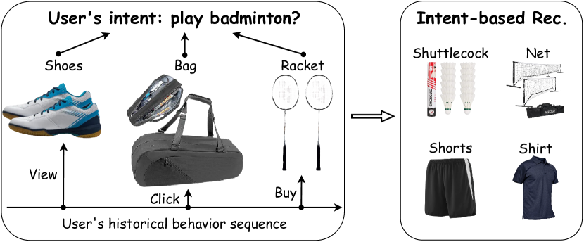
Figure 1: Intent learning in recommendation.

The optimization paradigm of the recent representative intent learning methods can be summarized as a generalized Expectation Maximization (EM) framework, as shown in Figure 2. To be specific, at the E-step, clustering algorithms are adopted to learn the latent intents from users’ behavior embeddings. And, at the M-step, the self-supervised learning methods are utilized to embed the users’ behavior sequences. The optimizations of these two steps are conducted alternately, achieving promising performance.

However, we highlight two issues in this complex and tedious alternating optimization. (1) At the E-step, we need to apply the clustering algorithm on the whole data, limiting the model’s scalability, especially in large-scale industrial scenarios, e.g., apps with billion users. (2) In the EM framework, the optimization of behavior learning and the clustering algorithm are separated, leading to sub-optimal performance and increasing the implementation difficulty.

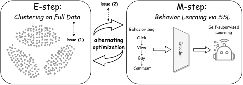
Figure 2: The general optimization framework of intent learning.

To this end, we propose a novel intent learning model named ELCRec via integrating representation learning into an End-to-end Learnable Clustering framework, for effective and efficient Recommendation. Specifically, the user’s behavioral process is first embedded into the latent space. Cluster centers, recognized as the users’ latent intents, are initialized as learnable neural network parameters. Then, a simple yet effective learnable clustering module is proposed to decouple users’ complex intents into different simple intent units by separating the cluster centers. Meanwhile, it makes the behavior embeddings close to cluster centers to guide the models to learn more accurate intents from users’ behaviors. This improves the model’s scalability and alleviates the issue (1) by optimizing the cluster distribution on mini-batch data. Furthermore, to further enhance the mutual promotion of representation learning and clustering, we present intent-assisted contrastive learning to integrate the cluster centers as self-supervision signals for representation learning. These settings unify behavior learning and clustering optimization in an end-to-end optimizing framework, improving recommendation performance and simplifying deployment. Therefore, the issue (2) has been also solved. The contributions of this paper are summarized as follows.

• We innovatively promote the existing optimization framework of intent learning by unifying behavior representation learning and clustering optimization.

• A new intent learning model termed ELCRec is proposed with a simple yet effective learnable cluster module and intent-assisted contrastive learning.

• Comprehensive experiments and theoretical analyses demonstrate advantages of ELCRec from six perspectives, including superiority, effectiveness, efficiency, sensitivity, convergence, and visualization.

• We successfully deployed it on industrial recommendation system with 130 million page views and achieve promising results, providing various practical insights.

2 Related Work

We provide a brief overview of the related work for this paper. It can be divided into three parts, including sequential recommendation, intent learning, and clustering algorithms. At first, Sequential Recommendation (SR) focuses on recommending relevant items to users based on their historical behavior sequences. In addition, intent learning has emerged as a promising and practical technique in recommendation systems. It aims to capture users’ latent intents to achieve better user understanding and item recommendation. Lastly, clustering algorithms play a crucial role in recommendation systems since they can identify patterns and similarities in the users or items. Due to the limitation of the pages, we introduce the detailed related methods in the Appendix A.1.

3 Methodology

We present our proposed framework, ELCRec, in this section. Firstly, we provide the necessary notations and task definition. Secondly, we analyze and identify the limitations of existing intent learning. Finally, we propose our solutions to address these challenges.

3.1 Basic Notation

In a recommendation system, $\mathcal{U}$ denotes the user set, and $\mathcal{V}$ denotes the item set. For each user $u\in\mathcal{U}$, the historical behaviors are described by a sequence of interacted items $S^{u}=[s_{1}^{u},s_{2}^{u},...,s_{t}^{u},...,s_{|S^{u}|}^{u}]$. $S^{u}$ is sorted by time. $|S^{u}|$ denotes the interacted items number of user $u$. $s^{u}_{t}$ denotes the item which is interacted with user $u$ at $t$ step. In practice, during sequence encoding, the historical behavior sequences are limited with a maximum length $T$ (Hidasi et al., 2015; Kang & McAuley, 2018; Chen et al., 2022). The sequences truncated and remain the most recent $T$ interacted items if the length is greater than $T$. Besides, the shorter sequences are filled with “padding” items on the left until the length is $T$. Due to the limitation of the pages, we list the basic notations in Table 7 of the Appendix A.2.

3.2 Task Definition

Given the user set $\mathcal{U}$ and the item set $\mathcal{V}$, the recommendation system aims to precisely model the user interactions and recommend items to users. Take user $u$ for an example, the sequence encoder firstly encodes the user’s historical behaviors $S^{u}$ to the latent embedding $\mathbf{E}^{u}$. Then, based on the historical behavior embedding, the target of the recommendation task is to predict the next item that is most likely interacted with by user $u$ at $|S^{u}|+1$ step.

3.3 Problem Analyses

Among the techniques in recommendation, intent learning has become an effective technique to understand users. We summarize the optimization procedure of the intent learning as the Expectation Maximization (EM) framework as shown in Figure 2. It contains two steps including E-step and M-step. These two steps are conducted alternately, mutually promoting each other. However, we find two issues of the existing optimization framework as follows.

1. In the process of E-step, it needs to perform a clustering algorithm on the full data, easily leading to out-of-memory or long-running time problems. It restricts the scalability of the model on large-scale industrial data.

2. The alternative optimization approach within the EM framework separates the learning process for behaviors and intents, leading to sub-optimal performance and increased implementation complexity. Also, it limits the training and inference on the real-time data. That is, when users’ behaviors and intents change over time, there is a long lag in the training and inference process

Therefore, we aim to develop a new optimization framework for intent learning to solve issue (1) and issue (2). For the issue (1), a new learnable online clustering method is the key solution. For the issue (2), we need to break the alternative optimization in the EM framework and build an end-to-end optimization framework.

3.4 Proposed Method

To this end, we present a new intent learning method termed ELCRec by unifying sequence representation learning into an End-to-end Learnable Clustering framework, for Recommendation. It contains three parts, including behavior encoding, end-to-end learnable cluster module, and intent-assisted contrastive learning.

3.4.1 Behavior Encoding

In this process, we aim to encoder the users’ behavior sequences. Concretely, given the user set $\mathcal{U}$, the item set $\mathcal{V}$, and the users’ historical behavior sequence set $\{S^{u}\}_{u=1}^{|\mathcal{U}|}$, the behavior encoder $\mathcal{F}$ embeds the behavior sequences of each user $u$ into the latent space as follows.

$$\mathbf{E}^{u}=\mathcal{F}(S^{u}),$$ (1)

where $\mathbf{E}^{u}\in\mathbb{R}^{|S^{u}|\times d^{\prime}}$ denotes the behavior sequence embedding of user $u$, $d^{\prime}$ is the dimension number of latent features, and $|S^{u}|$ denotes the length of behavior sequence of user $u$. Note that the behavior sequence lengths of different users are different. Therefore, all user behavior sequences are pre-processed to the sequences with the same length $T$ by padding or truncating. The encoder $\mathcal{F}$ is designed as a Transformer-based (Vaswani et al., 2017) architecture. Subsequently, to summarize the behaviors over different time of each user, the behavior sequence embedding is aggregated by the concatenate pooling function $\mathcal{P}$ as follows.

$$\mathbf{h}_{u}=\mathcal{P}(\mathbf{E}^{u})=\text{concat}(\mathbf{e}^{u}_{1}||...\mathbf{e}^{u}_{i}...||\mathbf{e}^{u}_{T}),$$ (2)

where $\mathbf{e}^{u}_{i}\in\mathbb{R}^{1\times d^{\prime}}$ denotes the embedding of user behavior at $i$-th step and $\mathbf{h}_{u}\in\mathbb{R}^{1\times Td^{\prime}}$ denotes the aggregated behavior embedding of user $u$. We re-denote $Td^{\prime}$ as $d$ for convenience. By encoding and aggregation, we obtain the behavior embeddings of all users $\mathbf{H}\in\mathbb{R}^{|\mathcal{U}|\times d}$.

3.4.2 End-to-end Learnable Cluster Module

After behavior encoding, we guide the model to learn the users’ latent intents from the behavior embeddings. To this end, an end-to-end learnable cluster module (ELCM) is proposed to break the alternative optimization in the previous mentioned EM framework. This module can groups the uers’ behaviors embeddings into various clusters, which represent the users’ latent intents or interests. Concretely, at first, the cluster centers $\mathbf{C}\in\mathbb{R}^{k\times d}$ are initialized as the learnable neural parameters, i.e., the tensors with gradients. Then, we design a simple yet effective clustering loss to train the networks and cluster centers as formulated as follows.

$$\mathcal{L}_{\text{cluster}} =\underbrace{\frac{-1}{(k-1)k}\sum_{i=1}^{k}\sum_{j=1,j\neq i}^{k}\left\|\hat{\mathbf{c}}_{i}-\hat{\mathbf{c}}_{j}\right\|_{2}^{2}}_{\text{Intent Decoupling}}+$$ (3)

$$\underbrace{\frac{1}{bk}\sum_{i=1}^{b}\sum_{j=1}^{k}\left\|\hat{\mathbf{h}}_{i}-\hat{\mathbf{c}}_{j}\right\|_{2}^{2}}_{\text{Intent-behavior Alignment}},$$

where $\hat{\mathbf{h}}_{i}=\mathbf{h}_{i}/\|\mathbf{h}_{i}\|_{2},\hat{\mathbf{c}}_{i}=\mathbf{c}_{i}/\|\mathbf{c}_{i}\|_{2}$. In Eq. (3), $k$ denotes the number of clusters (intents), and $b$ denotes the batch size. $\mathbf{h}_{i}\in\mathbb{R}^{1\times d}$ denotes the $i$-th user’s behavior embedding and $\mathbf{c}_{j}\in\mathbb{R}^{1\times d}$ denotes the $j$-th cluster center. For better network convergence, we constrain the behavior embeddings and cluster center embeddings to distribute on a unit sphere. Concretely, we apply the $l$-2 normalization to both the user behavior embeddings $\mathbf{H}$ and the cluster centers $\mathbf{C}$ during calculate the clustering loss $\mathcal{L}_{\text{cluster}}$.

In the proposed clustering loss, the first term is designed to disentangle the complex users’ intents into simple intent units. Technically, it pushes away different cluster centers, therefore reducing the overlap between different clusters (intents). The time complexity and space complexity of this term are $\mathcal{O}(k^{2}d)$ and $\mathcal{O}(kd)$, respectively. The number of users’ intents is vastly less than the number of users, i.e., $k\ll|\mathcal{U}|$. Therefore, the first term of the proposed clustering loss will not bring significant time or space costs.

In addition, the second term of the proposed clustering loss aims to align the users’ latent intents with the behaviors by pulling the behavior embeddings to the cluster centers. This design makes the in-class cluster distribution more compact and guides the network to condense similar behaviors into one intention. Also, on another aspect, it forces the model to learn users’ intents from behavior embeddings. Note that the behavior embedding $\mathbf{h}_{i}$ is pulled to all center centers $\mathbf{c}_{j},j=1,...,k$ rather than the nearest cluster center. The main reason is that the practical clustering algorithm is imperfect, and pulling to the nearest center easily leads to the confirmation bias problem (Nickerson, 1998). To this end, the proposed clustering loss $\mathcal{L}_{\text{cluster}}$ aims to optimize the clustering distribution in an adversarial manner by pulling embeddings together to cluster centers while pushing different cluster centers away. Besides, it enables the optimization of this term via mini-batch samples, avoiding performance clustering algorithms on the whole data. Time complexity and space complexity of the second term are $\mathcal{O}(bkd)$ and $\mathcal{O}(bk+bd+kd)$, respectively. Since the batch size is essentially less than the number of users, namely, $b\ll|\mathcal{U}|$, the second term of clustering loss $\mathcal{L}_{\text{cluster}}$ alleviates the considerable time or space costs. Besides, theoretically, based on the Rademacher complexity, we investigate the generalization bounds of $\mathcal{L}_{\text{cluster}}$ in the Appendix A.3.

In the existing EM optimization framework, the clustering algorithm needs to be applied on the entire users’ behavior embeddings $\mathbf{H}\in\mathbb{R}^{|\mathcal{U}|\times d}$. Take the classical $k$-Means clustering as an example, at each E-step, it leads to $\mathcal{O}(t|\mathcal{U}|kd)$ time complexity and $\mathcal{O}(|\mathcal{U}|k+|\mathcal{U}|d+kd)$ space complexity, where $t$ denote the iteration steps of $k$-Means clustering algorithm. We find that, at each step, the time and space complexity is linear to the number of users, thus leading to out-of-memory or running time problems (issue (1)), especially on large-scale industrial data, e.g., applications with millions or billions of users.

Fortunately, our proposed end-to-end learnable cluster module can solve this issue (1). By summarising previous analyses, we draw that the overall time and space complexity of calculating the clustering loss $\mathcal{L}_{\text{cluster}}$ are $\mathcal{O}(bkd+k^{2}d+bd)$ and $\mathcal{O}(bk+bd+kd)$, respectively. They are both linear to the batch size $b$ at each step, enabling the model’s scalability. Besides, the proposed module is plug-and-play and easily deployed in real-time large-scale industrial systems. We provide detailed evidence and practical insights in Section 5. The proposed ELCM can not only improve the recommendation performance (See Section 4.2 & 4.3) but also promote efficiency (See Section 4.4).

3.4.3 Intent-assisted Contrastive Learning

Next, we aim to enhance further the mutual promotion of behavior learning and clustering. To this end, Intent-assisted contrastive learning (ICL) is proposed by adopting cluster centers as self-supervision signals for behavior learning.

Firstly, we conduct contrastive learning among the behavior sequences. The new views of the behavior sequences are constructed via sequential augmentations, including mask, crop, and reorder. The two views of behavior sequence of user $u$ are denoted as $(S^{u})^{v1}$ and $(S^{u})^{v2}$. According to Section 3.4.1, the behaviors are encoded to the behavior embeddings $\mathbf{h}_{u}^{v1},\mathbf{h}_{u}^{v2}\in\mathbb{R}^{1\times d}$. Then, the sequence contrastive loss of user $u$ is formulated as follows.

$$\mathcal{L}_{\text{seq\_cl}}^{u}=$$ (4)

$$-\left(\text{log}\frac{e^{\text{sim}(\mathbf{h}_{u}^{v1},\mathbf{h}_{u}^{v2})}}{\sum_{\text{neg}}e^{\text{sim}(\mathbf{h}_{u}^{v1},\mathbf{h}_{\text{neg}})}}+\text{log}\frac{e^{\text{sim}(\mathbf{h}_{u}^{v1},\mathbf{h}_{u}^{v2})}}{\sum_{\text{neg}}e^{\text{sim}(\mathbf{h}_{u}^{v2},\mathbf{h}_{\text{neg}})}}\right),$$

where “sim” denotes the dot-product similarity, “neg” denotes the negative samples. Here, the same sequence with different augmentations is recognized as the positive sample pairs, and the other sample pairs are recognized as the negative sample pairs. By minimizing $\mathcal{L}_{\text{seq\_cl}}=\sum_{u}\mathcal{L}_{\text{seq\_cl}}^{u}$, the similar behaviors are pulled together, and the others are pushed away from each other, therefore enhancing the representation capability of users’ behaviors. During this process, the learned cluster centers $\mathbf{C}\in\mathbb{R}^{k\times d}$ are adopted as the self-supervision signals. We first query the index of the assigned cluster of $\mathbf{h}_{u}^{v1}$ as follows.

$$idx=\mathop{\arg\min}\limits_{i}(\left\|\mathbf{c}_{i}-\mathbf{h}_{u}^{v1}\right\|_{2}^{2}),$$ (5)

where $\mathbf{c}_{i}\in\mathbb{R}^{1\times d}$ denotes the $i$-th cluster (intent) center embedding. Then, the intent information is fused to the user behavior during the sequence contrastive learning. Here, we consider two optional fusion strategies, including the concatenate fusion $\mathbf{h}_{u}^{v1}=\text{concat}(\mathbf{h}_{u}^{v1}||\mathbf{c}_{idx})$ and the shift fusion $\mathbf{h}_{u}^{v1}=\mathbf{h}_{u}^{v1}+\mathbf{c}_{idx}$. A similar operation is applied to the second view of the behavior embedding $\mathbf{h}_{u}^{v2}$. After fusing the intent information to user behaviors, the neural networks are trained by minimizing $\mathcal{L}_{\text{seq\_cl}}$.

In addition, to further collaborate intent learning and sequential representation learning, we conduct contrastive learning between the user’s behaviors and the learnable intent centers. The intent contrastive loss is formulated as follows.

$$\mathcal{L}_{\text{intent\_cl}}^{u}=$$ (6)

$$-\left(\text{log}\frac{\min_{i}e^{\text{sim}(\mathbf{h}_{u}^{v1},\mathbf{c}_{i})}}{\sum_{\text{neg}}e^{\text{sim}(\mathbf{h}_{u}^{v1},\mathbf{c}_{\text{neg}})}}+\text{log}\frac{\min_{i}e^{\text{sim}(\mathbf{h}_{u}^{v2},\mathbf{c}_{i})}}{\sum_{\text{neg}}e^{\text{sim}(\mathbf{h}_{u}^{v2},\mathbf{c}_{\text{neg}})}}\right),$$

where $\mathbf{h}_{u}^{v_{1}},\mathbf{h}_{u}^{v_{2}}$ are two-view behavior embedding of the user $u$. Besides, “neg” denotes the negative behavior-intent pairs among all pairs. Here, we regard the behavior embedding and the corresponding nearest intent center as the positive pair and others as negative pairs. By minimizing the intent contrastive loss $\mathcal{L}_{\text{intent\_cl}}=\sum_{u}\mathcal{L}_{\text{intent\_cl}}^{u}$, behaviors with the same intents are pulled together, but behaviors with different intents are pushed away. In summary, the objective of ICL is formulated as follows.

$$\mathcal{L}_{\text{icl}}=\mathcal{L}_{\text{seq\_cl}}+\mathcal{L}_{\text{intent\_cl}}.$$ (7)

The effectiveness of ICL is verified in Section 4.3. With the proposed ELCM and ICL, we develop a new end-to-end optimization framework for intent learning, improving performance and convenience. Now, the issue (2) is solved.

3.4.4 Overall Objective

The neural networks and learnable clusters are trained with multiple tasks, including intent learning, intent-assisted contrastive learning, and next-item prediction. The intent learning task aims to capture the users’ underlying intents. Besides, intent-assisted contrastive learning aims to collaborate with intent learning and behavior learning. In addition, the next-item prediction task is a widely used task for recommendation systems. In summary, the overall objective of the proposed ELCRec is formulated as follows.

$$\mathcal{L}_{\text{overall}}=\mathcal{L}_{\text{next\_item}}+0.1\times\mathcal{L}_{\text{icl}}+\alpha\times\mathcal{L}_{\text{cluster}},$$ (8)

where $\mathcal{L}_{\text{next\_item}}$, $\mathcal{L}_{\text{icl}}$, and $\mathcal{L}_{\text{cluster}}$ denotes the next item prediction loss, intent-assisted contrastive learning loss, and clustering loss, respectively. $\alpha$ is a trade-off hyper-parameter. We present the overall algorithm process of the proposed ELCRec method in Algorithm 1.

Algorithm 1 End-to-end Learnable Clustering Framework for Recommendation (ELCRec)

Input: user set $\mathcal{U}$; item set $\mathcal{V}$; historical behavior sequences $\{\mathcal{S}^{u}\}_{u=1}^{|\mathcal{U}|}$; cluster number $k$; epoch number $E$; learning rate; trade-off parameter $\alpha$.
Output: Trained ELCRec.

1:  Initialize model parameters in encoders.

2:  for $\text{epoch}=1,2,...,E$ do

3:    for $\text{u}=1,2,...,|\mathcal{U}|$ do

4:      Obtain $u$-th user’s behavior sequence embedding $\mathbf{E}^{u}\in\mathbb{R}^{|\mathcal{S}^{u}|\times d^{\prime}}$ via encoding $\mathcal{S}^{u}$ in Eq. (1).

5:      Obtain $u$-th user’s aggregated behavior embedding $\mathbf{h}_{u}\in\mathbb{R}^{1\times d}$ via aggregating $\mathbf{E}^{u}$ in Eq. (2)

6:    end for

7:    Obtain behavior embeddings of all users $\mathbf{H}\in\mathbb{R}^{|\mathcal{U}|\times d}$.

8:    Initialize cluster centers $\mathbf{C}\in\mathbb{R}^{k\times d}$ as learnable.

9:    Calculate clustering loss to conduct intent learning.

10:    Generate two views of behaviors via data augmentations.

11:    Encode the two views of the behavior sequences.

12:    Calculate $\mathcal{L}_{\text{seq\_cl}}$ to conduct behavior contrastive learning.

13:    Query cluster index of the behavior embeddings via Eq. (5).

14:    Fuse the intent information to behavior embeddings.

15:    Calculate $\mathcal{L}_{\text{intent\_cl}}$ to conduct intent contrastive learning.

16:    Calculate $\mathcal{L}_{\text{next\_item}}$ to conduct next item prediction task.

17:    Minimize $\mathcal{L}_{\text{overall}}$ to train the model in Eq. (8).

18:  end for

19:  Return Well-trained ELCRec model.

4 Experiment

This section aims to comprehensively evaluate our ELCRec by answering the following research questions (RQ).

1. Superiority: does ELCRec outperform the existing state-of-the-art sequential recommendation methods?

2. Effectiveness: are the end-to-end learnable cluster module and intent-assisted contrastive learning effective?

3. Efficiency: how about the time and memory efficiency of the proposed ELCRec?

4. Sensitivity: what is the performance of the proposed method with different hyper-parameters?

5. Convergence: will the proposed loss function and the recommendation performance converge well?

6. Visualization: Can the visualized learned embeddings reflect the promising results?

We answer RQ(i), (ii), (iii) in Section 4.2, 4.3, 4.4, respectively. Due to the limited pages, RQ(iv), (v), (vi) are answered in the Appendix A.5, A.6, and A.7 respectively.

4.1 Experimental Setup

4.1.1 Experimental Environment

Experimental results on the public benchmarks are obtained from the desktop computer with one NVIDIA GeForce RTX 4090 GPU, six 13th Gen Intel(R) Core(TM) i9-13900F CPUs, and the PyTorch platform.

Table 1: Statistical information of four public datasets.

Dataset	#User	#Item	#Action	Avg. Len.	Sparsity
Sports	35,598	18,357	0.3M	8.3	99.95%
Beauty	22,363	12,101	0.2M	8.9	99.95%
Toys	19,412	11,924	0.17M	8.6	99.93%
Yelp	30,431	20,033	0.3M	8.3	99.95%

4.1.2 Public Benchmark

We performed our experiments on four public benchmarks: Sports, Beauty, Toys, and Yelp. The Sports, Beauty, and Toys datasets are subcategories of the Amazon Review Dataset (McAuley et al., 2015). The Sports dataset contains reviews for sporting goods, the Beauty dataset contains reviews for beauty products, and the Toys dataset contains toy reviews. On the other hand, the Yelp dataset focuses on business recommendations and is provided by Yelp company. Table 1 summarizes the datasets’ details. We only kept datasets where all users and items have at least five interactions. Besides, we adopted the dataset split settings used in the previous method (Chen et al., 2022).

4.1.3 Evaluation Metric

To evaluate ELCRec, we adopt two groups of metrics, including Hit Ratio@$k$ (HR@$k$) and Normalized Discounted Cumulative Gain@$k$ (NDCG@$k$), where $k\in\{5,20\}$.

4.1.4 Compared Baseline

We compare our method with nine baselines including BPR-MF (Rendle et al., 2012), GRU4Rec (Hidasi et al., 2015), Caser (Tang & Wang, 2018), SASRec (Kang & McAuley, 2018), DSSRec (Ma et al., 2020), BERT4Rec (Sun et al., 2019), S3-Rec (Zhou et al., 2020), CL4SRec (Xie et al., 2022), and ICLRec (Chen et al., 2022). Detailed introductions to these methods are in the Appendix A.1.2.

4.1.5 Implementation Detail

For the baselines, we adopt their original code with the original settings to reproduce the results on four benchmarks. Due to page limitation, the detailed implementation of the baselines are listed in Appendix A.8. The proposed method, ELCRec, was implemented using the PyTorch deep learning platform. In the Transformer encoder, we employed self-attention blocks with two attention heads. The latent dimension, denoted as $d$, was set to 64, and the maximum sequence length, denoted as $T$, was set to 50. We utilized the Adam optimizer with a learning rate of 1e-3. The decay rate for the first moment estimate was set to 0.9, and the decay rate for the second moment estimate was set to 0.999. The cluster number, denoted as $k$, was set to 256 for the Yelp and Beauty datasets and 512 for the Sports and Toys datasets. The trade-off hyper-parameter, denoted as $\alpha$, was set to 1 for the Sports and Toys datasets, 0.1 for the Yelp dataset, and 10 for the Beauty dataset. During training, we monitored the training process via the Weights & Biases.

4.2 Superiority

In this section, we aim to answer the research question (i) and demonstrate the superiority of ELCRec. To be specific, we compare ELCRec with nine state-of-the-art recommendation baselines (Rendle et al., 2012; Hidasi et al., 2015; Tang & Wang, 2018; Kang & McAuley, 2018; Ma et al., 2020; Sun et al., 2019; Zhou et al., 2020; Xie et al., 2022; Chen et al., 2022). Experimental results are the mean values of three runs. As shown in Table 2, the bold values and underlined values denote the best and runner-up results, respectively. From these results, we have four conclusions as follows.

1. The non-sequential model BPR-MF (Rendle et al., 2012) has not achieved promising performance since the shallow method lacks the representation learning capability of users’ historical behaviors.

2. The conventional sequential methods (Hidasi et al., 2015; Tang & Wang, 2018; Kang & McAuley, 2018) improve the recommendation via different DNNs such as CNN (Krizhevsky et al., 2012), RNN (Zaremba et al., 2014), and Transformer (Vaswani et al., 2017). But they perform worse since limiting self-supervision.

3. The recent methods (Sun et al., 2019; Zhou et al., 2020; Xie et al., 2022) enhance the self-supervised capability of models via the self-supervised learning techniques. However, they neglect the underlying users’ intent, thus leading to sub-optimal performance.

4. More recently, the intent learning methods (Li et al., 2019; Cen et al., 2020; Li et al., 2021a; Chen et al., 2022; Li et al., 2023b, 2024; Bai et al., 2024) have been proposed to mine users’ underlying intent to assist recommendation. Motivated by their success, we propose a new intent learning method termed ELCRec. Befitting from the strong intent learning capability of ELCRec, it surpasses all other intent learning methods.

To further verify the superiority of ELCRec, we conduct the $t$-test between the best and runner-up methods. As shown in Table 2, the most $p$-value is less than 0.05 except HR@5 on the Toys dataset. It indicates that ELCRec significantly outperforms runner-up methods. Overall, the extensive experiments demonstrate the superiority of ELCRec. In addition, we also conduct comparison experiments on recommendation datasets of other domains, including movie recommendation and news recommendation, as shown in the Appendix A.4.1 and A.4.2. These experimental results demonstrate a broader applicability of our proposed ELCRec.

Table 2: Recommendation performance on benchmarks. Bold values and underlined values denote the best and runner-up results. ^∗ indicates that, in the $t$-test, the best method significantly outperforms the runner-up with $p<0.05$. ”-” indicates models do not converge.

Dataset	Metric	BPR-MF	GRU4Rec	Caser	SASRec	BERT4Rec	DSSRec	S3-Rec	CL4SRec	DCRec	MAERec	IOCRec	ICLRec	ELCRec	Impro.	$p$-value
Sports	HR@5	0.0141	0.0162	0.0154	0.0206	0.0217	0.0214	0.0121	0.0217	0.0172	0.0225	0.0246	0.0263	0.0286	8.75%$\uparrow$	2.34e-6∗
	HR@20	0.0323	0.0421	0.0399	0.0497	0.0604	0.0495	0.0344	0.0540	0.0357	0.0488	0.0641	0.0630	0.0648	1.09%$\uparrow$	2.29e-4∗
	NDCG@5	0.0091	0.0103	0.0114	0.0135	0.0143	0.0142	0.0084	0.0137	0.0118	0.0152	0.0162	0.0173	0.0185	6.94%$\uparrow$	3.54e-5∗
	NDCG@20	0.0142	0.0186	0.178	0.0216	0.0251	0.0220	0.0146	0.0227	0.0170	0.0225	0.0280	0.0276	0.0286	2.14%$\uparrow$	7.87e-3∗
Beauty	HR@5	0.0212	0.0111	0.0251	0.0374	0.0360	0.0410	0.0189	0.0423	0.0368	0.0414	0.0408	0.0495	0.0529	6.87% $\uparrow$	3.18e-6∗
	HR@20	0.0589	0.0478	0.0643	0.0901	0.0984	0.0914	0.0487	0.0994	0.0674	0.0854	0.0916	0.1072	0.1079	0.65%$\uparrow$	3.30e-3∗
	NDCG@5	0.0130	0.0058	0.0145	0.0241	0.0216	0.0261	0.0115	0.0281	0.0269	0.0283	0.0245	0.0326	0.0355	8.90%$\uparrow$	4.48e-6∗
	NDCG@20	0.0236	0.0104	0.0298	0.0387	0.0391	0.0403	0.0198	0.0441	0.0357	0.0407	0.0444	0.0491	0.0509	3.67%$\uparrow$	9.08e-6∗
Toys	HR@5	0.0120	0.0097	0.0166	0.0463	0.0274	0.0502	0.0143	0.0526	0.0399	0.0477	0.0311	0.0586	0.0585	0.17%$\downarrow$	1.22e-1
	HR@20	0.0312	0.0301	0.0420	0.0941	0.0688	0.0975	0.0235	0.1038	0.0679	0.0904	0.0781	0.1130	0.1138	0.71%$\uparrow$	4.20e-3∗
	NDCG@5	0.0082	0.0059	0.0107	0.0306	0.0174	0.0337	0.0123	0.0362	0.0296	0.0336	0.0197	0.0397	0.0403	1.51%$\uparrow$	2.87e-4∗
	NDCG@20	0.0136	0.0116	0.0179	0.0441	0.0291	0.0471	0.0162	0.0506	0.0374	0.0458	0.0330	0.0550	0.0560	1.82%$\uparrow$	3.72e-5∗
Yelp	HR@5	0.0127	0.0152	0.0142	0.0160	0.0196	0.0171	0.0101	0.0229	-	0.0166	0.0222	0.0233	0.0236	1.29% $\uparrow$	7.81e-3∗
	HR@20	0.0346	0.0371	0.0406	0.0443	0.0564	0.0464	0.0314	0.0630		0.0460	0.0640	0.0645	0.0653	1.24%$\uparrow$	3.73e-4∗
	NDCG@5	0.0082	0.0091	0.0080	0.0101	0.0121	0.0112	0.0068	0.0144		0.0105	0.0137	0.0146	0.0150	2.74%$\uparrow$	1.23e-2∗
	NDCG@20	0.0143	0.0145	0.0156	0.0179	0.0223	0.0193	0.0127	0.0256		0.0186	0.0263	0.0261	0.0266	1.14%$\uparrow$	6.82e-3∗

4.3 Effectiveness

This section is dedicated to answering the research question (ii) and evaluating the effectiveness of the End-to-end Learnable Cluster Module (ELCM) and Intent-assisted Contrastive Learning (ICL). To achieve this, we conducted meticulous ablation studies on four benchmarks. Figure 3 illustrates the experimental results. In each sub-figure, “B”, “B+ICL,” “B+ELCM,” and “ELCRec” correspond to the backbone, backbone with ICL, backbone with ELCM, and backbone with both ICL and ELCM, respectively. Through the ablation studies, we draw three key conclusions.

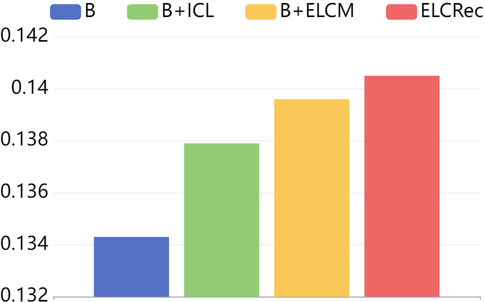
(a) Sports

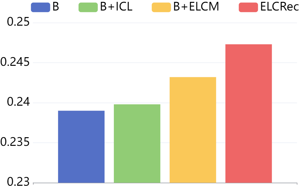
(b) Beauty

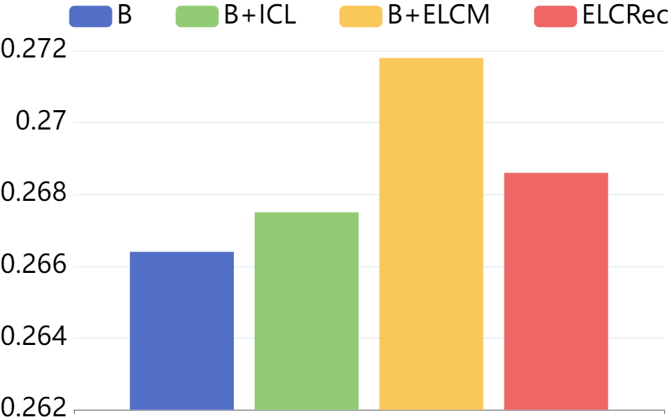
(c) Toys

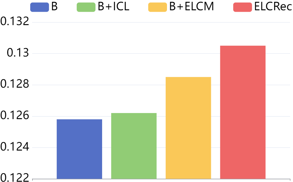
(d) Yelp

Figure 3: Ablation studies of the proposed end-to-end learnable cluster module (ELCM) and the intent-assisted contrastive learning (ICL). The results are the sum of four metrics, including HR@5, HR@20, NDCG@5, and NDCG@20.

1. “B+ICL” outperforms the backbone “B” on all four benchmarks. It indicates that the proposed ICL effectively improves behavior learning.

2. “B+ELCM” surpasses the backbone “B” significantly on all benchmarks. This phenomenon demonstrates that our proposed end-to-end learnable cluster module helps the model better capture the users’ underlying intents, thus improving recommendation performance.

3. ELCRec achieves the best performance on three out of four datasets. It shows the effectiveness of the combination of these two modules. On the Toys dataset, ELCRec can outperform the “B” and “B+ICL” but perform worse than “B+ELCM”. This phenomenon indicates it is worth researching the better collaboration of these two modules in the future. To summarize, these extensive ablation studies verify the effectiveness of the proposed intent-assisted contrastive learning and end-to-end learnable cluster module in ELCRec.

Table 3: Running Time costs. Bold values denote better results.

Dataset	Sports	Beauty	Toys	Yelp	Avg.
ICLRec	5282	3770	4374	4412	4460
ELCRec	5360	2922	4124	4151	4139
Impro.	1.48% $\uparrow$	22.49% $\downarrow$	5.72% $\downarrow$	5.92% $\downarrow$	7.18% $\downarrow$

Table 4: GPU memory costs. Bold values denote better results.

Dataset	Sports	Beauty	Toys	Yelp	Avg.
ICLRec	1944	1798	2887	3671	2575
ELCRec	1781	1594	2555	3383	2328
Impro.	8.38% $\downarrow$	11.35% $\downarrow$	11.50% $\downarrow$	7.85% $\downarrow$	9.58% $\downarrow$

4.4 Efficiency

We test the efficiency of ELCRec on four benchmarks and answer the research question (iii). Concretely, the efficiency contains two perspectives, including training time costs (in second) and GPU memory costs (in MB). We have two observations as follows. (a) ELCRec can speed up ICLRec on three out of four datasets (See Table 3). Overall, on four datasets, the training time is decreased by 7.18% on average. The reason is that our proposed end-to-end optimization of intent learning breaks the alternative optimization of the EM framework, saving computation costs. (b) The results demonstrate that the GPU memory costs of our ELCRec are lower than that of ICLRec on four datasets (See Table 4). On average, the GPU memory costs are decreased by 9.58%. It is because we enable the model to conduct intent learning via the mini-batch users’ behaviors. Therefore, in summary, we demonstrate the efficiency of our proposed ELCRec from both time and memory aspects.

5 Application

Our proposed ELCRec is versatility and plug-and-play. Benefiting its advantages, we aim to apply it to real-time large-scale industrial recommendation systems with millions of users. First, we introduce the background and settings of the application. Then, we conduct extensive A/B testing and analyze the experimental results. Besides, due to the page limitation, we provide deployment details and practical insights in Appendix A.9 and A.10, respectively.

5.1 Application Background

The applied scenario is the livestreaming recommendation on the front page of the Alipay app. The user view (UV) and page view (PV) of this application are about 50 million and 130 million, respectively. Note that most users are new to this application, therefore leading to the sparsity of users’ behaviors. To solve this cold-start problem in the recommendation system, we adopt our proposed method to group users and recommend items based on the groups. Concretely, due to the sparsity of users’ behaviors, we first replace the users’ behavior with the users’ activities features in this application and model them via the multi-gate mixture-of-expert (MMOE) model (Ma et al., 2018). Then, the end-to-end learnable cluster module is adopted to group the users into various groups. Through this module, the high-activity users and new users are grouped into different clusters, alleviating the cold-start issue and assisting in better recommendations. Besides, during the learning process of the cluster embeddings, the low-activity users can transfer to high-activity users, improving the overall users’ activities in the application. Eventually, the networks are trained with multiple tasks. In the next section, we conduct experiments to demonstrate the effectiveness of our proposed method on real-time large-scale industrial data.

5.2 A/B Testing on Real-time Large-scale Data

We conduct A/B testing on the real-time large-scale industrial recommendation system. The experimental results are listed in Table 5. We evaluate the models with two metric systems, including livestreaming metrics and merchandise metrics. livestreaming metrics contain Page View Click Through Rate (PVCTR) and Video View (VV). Merchandise metrics contain PVCTR and User View Click Through Rate (UVCTR). The results indicate that our method can improve the recommendation performance of the baseline by about 2%. Besides, the improvements are significant with $p<0.05$ in three out of four metrics.

Table 5: A/B testing on real-time large-scale industrial recommendation. Bold values denotes the significant improvements with $p<0.05$. The symbol “-” denotes business secret.

Method	Livestreaming Metrics		Merchandise Metrics
	PVCTR	VV	PVCTR	UVCTR
Baseline	-	-	-	-
Impro.	2.45% $\uparrow$	2.28% $\uparrow$	2.41% $\uparrow$	1.62% $\uparrow$

In addition, to further explore why our method can work well in real-time large-scale recommendation systems, we further analyze the recommendation performance on different user groups. The results are shown in Table 6. Based on the users’ activity, we classify them into five groups, including Pure New users (PN), New users (N), Low-Activity users (LA), Medium-Activity users (MA), and High-Activity users (HA). Compared with the general recommendation algorithms that are unfriendly to new users, the experimental results show that our module not only improves the recommendation performance of high-activity users but also improves the recommendation performance of new users. Therefore, it can alleviate the cold-start problem and construct a more friendly user ecology.

Table 6: Experimental results of different user groups. Bold values denotes the significant improvements with $p<0.05$.

Metric	PN	N	LA	MA	HA
PVCTR	6.96% $\uparrow$	1.67% $\uparrow$	1.98% $\uparrow$	0.35% $\uparrow$	19.02% $\uparrow$
VV	6.81% $\uparrow$	1.50% $\uparrow$	1.50% $\uparrow$	0.04% $\uparrow$	16.90% $\uparrow$

6 Conclusion

In this paper, we explore intent learning in recommendation systems. To be specific, we summarize and analyze two drawbacks of the existing EM optimization framework of intent learning. The complex and cumbersome alternating optimization limits the scalability and performance of existing methods. To this end, we propose a novel intent learning method termed ELCRec with an end-to-end learnable cluster module and intent-assisted contrastive learning. Extensive experiments on four benchmarks demonstrate ELCRec’s six abilities. In addition, benefiting from the versatility of ELCRec, we successfully apply it to the real-time large-scale industrial scenario and also achieve promising performance. Due to the limited pages, We discuss the limitations and future work of this paper in Appendix A.11.

Impact Statements

The requirement states: “This statement should be in a separate section at the end of the paper (co-located with Acknowledgements, before References), and does not count toward the paper page limit.”. To meet the requirement, we state as follows. This paper presents work whose goal is to advance the field of Machine Learning, Artificial Intelligence, and Data Mining. There are many potential societal consequences of our work, e.g., recommendation system development and user understanding in technical companies.

Appendix A Appendix

A.1 Detailed Related Work

A.1.1 Sequential Recommendation

Sequential Recommendation (SR) poses a significant challenge as it strives to accurately capture users’ evolving interests and recommend relevant items by learning from their historical behavior sequences. In the early stages, classical techniques such as Markov Chains and matrix factorization have assisted models (He & McAuley, 2016a; Rendle, 2010; Rendle et al., 2010) in learning patterns from past transactions. Deep learning has garnered significant attention in recent years and has demonstrated promising advancements across various domains, including vision and language. Inspired by the remarkable success of Deep Neural Networks (DNNs), researchers have developed a range of deep Sequential Recommendation (SR) methods. For instance, Caser (Tang & Wang, 2018) leverages Convolutional Neural Networks (CNNs) (Krizhevsky et al., 2012) to embed item sequences into an ”image” representation over time, enabling the learning of sequential patterns through convolutional filters. Similarly, GRU4Rec (Hidasi et al., 2015) utilizes Recurrent Neural Networks (RNNs) (Zaremba et al., 2014), specifically the Gated Recurrent Unit (GRU), to model entire user sessions. The Transformer architecture (Vaswani et al., 2017) has also gained significant popularity and has been extended to the recommendation domain. For example, SASRec (Kang & McAuley, 2018) employs a unidirectional Transformer to model users’ behavior sequences, while BERT4Rec (Sun et al., 2019) utilizes a bidirectional Transformer to encode behavior sequences from both directions. To enhance the time and memory efficiency of Transformer-based SR models, LSAN (Li et al., 2021b) introduces aggressive compression techniques for the original embedding matrix. Addressing the cold-start issue in SR models, ASReP (Liu et al., 2021b) proposes a pre-training and fine-tuning framework. Furthermore, researchers have explored the layer-wise disentanglement of architectures (Zhang et al., 2023b) and introduced novel modules like the Wasserstein self-attention module in STOSA (Fan et al., 2022) to model item-item position-wise relationships. In addition to Transformers, graph neural networks (Ye et al., 2023a; Zhang et al., 2022b; Li et al., 2023c; Chang et al., 2021) and multilayer perceptrons (Li et al., 2023a, 2022; Zhou et al., 2022) have also found applications in recommendation systems. More recently, Self-Supervised Learning (SSL) (Yu et al., 2023; Ren et al., 2023), particularly contrastive learning (Jing et al., 2023), has gained popularity due to its ability to learn patterns from large-scale unlabeled data. As a result, SSL-based SR models have been increasingly introduced. For instance, in CoSeRec (Liu et al., 2021a), Liu et al. propose two informative augmentation operators that leverage item correlations to generate high-quality views. They then utilize contrastive learning to bring positive sample pairs closer while pushing negative pairs apart. Subsequently, TiCoSeRec (Dang et al., 2023) is designed by considering the time intervals in the behavior sequences. Another contrastive SR method, ECL-SR (Zhou et al., 2023), ensures that the learned embeddings are sensitive to invasive augmentations while remaining insensitive to mild augmentations. Additionally, DCRec (Yang et al., 2023) addresses the issue of popularity bias through a debiased contrastive learning framework. Moreover, DuoRec (Qiu et al., 2022) is proposed to solve the representation degeneration problem in contrastive recommendation methods. Techniques such as hard negative mining (Fan et al., 2023; Petrov & Macdonald, 2023) have also proven beneficial for recommendation systems. Besides, motivated by the success of Mask Autoencoder (MAE) (He et al., 2022), MAERec (Ye et al., 2023b) is proposed with the graph masked autoencoder.

A.1.2 Intent Learning for Recommendation

The preferences of users towards items are implicitly reflected in their intents. Recent studies (Li et al., 2019; Cen et al., 2020; Li et al., 2021a; Chen et al., 2022; Li et al., 2023b, 2024; Bai et al., 2024) have highlighted the significance of users’ intents in the user understanding and enhancing the performance of recommendation systems. For instance, MCPRN (Wang et al., 2019b) introduces a mixture-channel method to model subsets of items with multiple purposes. Inspired by capsule networks (Sabour et al., 2017), MIND (Li et al., 2019) utilizes dynamic routing to learn users’ multiple interests. Furthermore, ComiRec (Cen et al., 2020) employs a multi-interest module to capture diverse interests from user behavior sequences, while the aggregation module combines items from different interests to generate overall recommendations. Besides, MITGNN (Liu et al., 2020) treats intents as translated tail entities and learns embeddings using graph neural networks. In addition, Pan et al. (Pan et al., 2020) propose an intent-guided neighbor detector to identify relevant neighbors, followed by a gated fusion layer that adaptively combines the current session with the neighbor sessions. Moreover, Ma et al. (Ma et al., 2020) aims to disentangle the intentions underlying users’ behaviors and construct sample pairs within the same intention. Meanwhile, the ASLI method (Tanjim et al., 2020) incorporates a temporal convolutional network layer to extract latent users’ intents. More recently, a general latent learning framework called ICLRec (Chen et al., 2022) is introduced, which utilizes contrastive learning and $k$-Means clustering to group the users’ behaviors to intents. Chang et al. (Chang et al., 2023) formulate users’ intents as latent variables and infer them based on user behavior signals using the Variational Auto Encoder (VAE) (Kingma & Welling, 2013). To mitigate noise caused by data augmentations in contrastive SR models, IOCRec (Li et al., 2023b) proposes building high-quality views at the intent level. Besides, ICSRec (Qin et al., 2024) is proposed to solve this issue by conducting contrastive learning on cross sub-sequences. DIMPS (Bai et al., 2024) aims to build dynamic and intent-oriented document representations for intent learning. PoMRec (Dong et al., 2024) insert the specific prompts into user interactions to make them adaptive to different learning objectives. Furthermore, Teddy (Li et al., 2024) is proposed by utilizing the intent trend and diversity.

A.1.3 Clustering Algorithm

Clustering is a fundamental and challenging task that aims to group samples into distinct clusters without supervision. By leveraging the power of unlabeled data, clustering algorithms have found applications in various domains, including computer vision (Chang et al., 2017), natural language processing (Aggarwal & Zhai, 2012), graph learning (Liu et al., 2023c), and recommendation systems (Chen et al., 2022; Qin et al., 2024). In the early stages, several traditional clustering methods (Hartigan & Wong, 1979; Von Luxburg, 2007; Reynolds, 2009; Ester et al., 1996; Rodriguez & Laio, 2014) were proposed. For instance, the classical $k$-Means clustering (Hartigan & Wong, 1979) iteratively updates cluster centers and assignments to group samples. Spectral clustering (Von Luxburg, 2007) constructs a similarity graph and utilizes eigenvalues and eigenvectors to perform clustering. Additionally, probability-based Gaussian Mixture Models (GMM) (Reynolds, 2009) assume that the data distribution is a mixture of Gaussian distributions and estimate parameters through maximum likelihood. In contrast, density-based methods (Ester et al., 1996; Rodriguez & Laio, 2014; Comaniciu & Meer, 2002) overcome the need for specifying the number of clusters as a hyperparameter. In recent years, the impressive performance of deep learning has sparked a growing interest in deep clustering (Li et al., 2021c; Ronen et al., 2022; Min et al., 2018; Asano et al., 2019; Qian et al., 2022; Li et al., 2020). For instance, Xie et al. propose DEC (Xie et al., 2016), a deep learning-based approach for clustering. They initialize cluster centers using $k$-Means clustering and optimize the clustering distribution using a Kullback-Leibler divergence clustering loss (Xie et al., 2016). IDEC (Guo et al., 2017) improves upon DEC by incorporating the reconstruction of original information from latent embeddings. JULE (Yang et al., 2016) and DeepCluster (Caron et al., 2018) both adopt an iterative approach, updating the deep network based on learned data embeddings and clustering assignments. SwAV (Caron et al., 2020), an online method, focuses on clustering data and maintaining consistency between cluster assignments from different views of the same image. DINO (Caron et al., 2021) introduces a momentum encoder to address representation collapse. Additionally, SeCu (Qian, 2023) proposes a stable cluster discrimination task and a hardness-aware clustering criterion. While deep clustering has been extensively applied to image data, it is also utilized in graph clustering (Liu et al., 2022c, d; Wang et al., 2019a; Yue et al., 2022; Pan et al., 2018; Liu et al., 2023c, d, b) and text clustering (Aggarwal & Zhai, 2012; Liu et al., 2022b; Jacksi et al., 2020; Saeed et al., 2020). However, the application of clustering-based recommendation (Chen et al., 2022; Qin et al., 2024) is relatively unexplored. Leveraging the unsupervised learning capabilities of clustering could benefit intent learning in recommendation systems.

A.2 Notation

Due to the page limitation of the regular paper, we summarize the basic notations used in this paper in Table 7.

Table 7: Basic notations.

Notation	Meaning
$\mathcal{U}$	User set
$\mathcal{V}$	Item set
$\{S^{u}\}_{u=1}^{|\mathcal{U}|}$	Users’ behavior sequence set
$(S^{u})^{v_{k}}$	Users’ behavior sequence set in view $k$
$d^{\prime}$	Dimension number of latent features
$d$	Dimension number of aggregated latent features
$b$	Batch size
$k$	Cluster number
$T$	Maximum sequence length
$\mathcal{L}_{\text{cluster}}$	Clustering loss
$\mathcal{L}_{\text{seq\_cl}}$	Behavior sequence contrastive loss
$\mathcal{L}_{\text{intent\_cl}}$	Intent contrastive loss
$\mathcal{L}_{\text{icl}}$	intent-assisted contrastive learning loss
$\mathcal{L}_{\text{next\_item}}$	Next item prediction loss
$\mathcal{L}_{\text{overall}}$	Overall loss of the proposed ELCRec
$\mathcal{F}$	Behavior Encoder
$\mathcal{P}$	Concatenate pooling function
$\mathbf{E}^{u}\in\mathbb{R}^{|S^{u}|\times d^{\prime}}$	Behavior sequence embedding of user $u$
$\mathbf{H}\in\mathbb{R}^{|\mathcal{U}|\times d}$	Behavior embeddings of all users
$\hat{\mathbf{H}}\in\mathbb{R}^{|\mathcal{U}|\times d}$	Normalized Behavior embeddings of all users
$\mathbf{H}^{v_{k}}\in\mathbb{R}^{|\mathcal{U}|\times d}$	Behavior embeddings of all users in view $v_{k}$
$\mathbf{C}\in\mathbb{R}^{k\times d}$	Learnable cluster center embeddings
$\hat{\mathbf{C}}\in\mathbb{R}^{k\times d}$	Normalized Learnable cluster center embeddings

A.3 Theoretical Analyses

In this subsection, we investigate the generalization bounds of the proposed clustering loss. Our analysis is based on the Rademacher complexity and investigates how it improves the generalization bound of the algorithm.

Without loss of generality, we have the following notation. Let $\mathbf{x}\in\mathcal{X}$ be the input, where $\mathbf{x}$ are generated from a underlying distribution $\mathbf{x}\sim\mathcal{P}$. Given $n$ training samples $\mathcal{S}\triangleq\{\boldsymbol{x}_{i}\}_{i\in[n]}$ generated from distribution $\mathcal{P}$, we denote its empirical distribution by $\mathcal{P}^{n}$. For every hyperparameter $\omega\in\Omega$, we define $\mathcal{F}_{\omega}$ as a distribution-dependent hypothesis space corresponding to the $\omega$, where $\Omega$ is a finite set of hyperparameters. $\mathcal{F}_{\omega}$ is defined as $\{f_{\omega}|f_{\omega}=\mathcal{A}_{\omega}(S),S\in\mathcal{S}\}$, where $\mathcal{A}_{\omega}$ is an algorithm that outputs the hypothesis $f_{\omega}$ given a dataset $S$.

In the subsequent analysis, we denote $\mathcal{L}_{\text{cluster}}(S,f_{\omega})=\ell\left(f_{\omega}(\mathbf{x},\mathbf{c})\right)$ as the proposed cluster loss $\mathcal{L}_{\text{cluster}}$ with the embedding $\mathbf{c}$. Let $u,v$ are the upper and lower bounds of the cluster loss respectively. In other words, $u\geq\ell\left(f_{\omega}(\mathbf{x},\mathbf{c})\right)\geq v$. In this paper, $u=4$ and $v=-4$. $\mathcal{R}^{\ell}_{n}{(\mathcal{F}_{\omega})}$ is the rademacher complexity of the set $\left\{\mathbf{x}\mapsto\ell(f_{\omega}(\mathbf{x},\mathbf{c}):f_{\omega}\in\mathcal{F}_{\omega}\right\}$. Besides, we have $\mathbb{E}_{\mathbf{x}\sim\mathcal{P}^{n}}\left[\ell(f_{\omega}(\mathbf{x},\mathbf{c})\right]=\frac{1}{n}\sum_{i=1}^{n}\ell\left(f_{\omega}(\mathbf{x}_{i},\mathbf{c})\right)$.

With the notation above, we have the following theorem.

Theorem A.1.

For any $\delta>0$ and $\omega\in\Omega$, for all $f_{\omega}\in\mathcal{F}_{\omega}$, with the probability at least $1-\delta$, we have:

$$\mathbb{E}_{\mathbf{x}\sim\mathcal{P}}[\ell(f_{\omega}(\mathbf{x},\mathbf{c}))]-\mathbb{E}_{\mathbf{x}\sim\mathcal{P}^{n}}[\ell(f_{\omega}(\mathbf{x},\mathbf{c}))]$$ (9)

$$\leq 2\sqrt{\frac{2\text{ln}\Pi_{\mathcal{F_{\omega}}}(n)}{n}}+(u-v)\sqrt{\frac{\text{ln}(1/\delta)}{2n}}.$$

where $\text{ln}\Pi_{\mathcal{F_{\omega}}}(n)$ denotes the growth function.

Remark A.2.

For each fixed $\mathcal{F}_{\omega}$, the generalization bound in Theorem 1 goes to zero since $\text{ln}\Pi_{\mathcal{F_{\omega}}}(n)/{n}\rightarrow 0$ and $\text{ln}(1/\delta)/{n}\rightarrow 0$ when $n\rightarrow\infty$. In conclusion, the generation gap is approximately $\mathcal{O}(1/{\sqrt{n}})$. Therefore, the generalization bound is promised.

To prove the above theorem, we need the following lemma.

Lemma A.3.

(Bartlett & Mendelson, 2002) Let $\mathcal{F}$ be a class of real-valued function that map from $\mathcal{X}$ to $[v,u]$. Let $\mathcal{D}$ be a probability distribution on $\mathcal{X}\times[v,u]$, and suppose that sample set $\mathbf{X}=\{x_{1},x_{2},\dots,x_{n}\}$ are chosen independently according to the distribution $\mathcal{D}$. For all $f\in\mathcal{F}$, with probability at least $1-\delta$, we have:

$$\Phi(S)\leq 2\mathcal{R}_{n}(\mathcal{F})+(u-v)\sqrt{\frac{\text{ln}(1/\delta)}{2n}},$$ (10)

where $\Phi(S)=\sup_{f\in\mathcal{F}}\left(\mathbb{E}_{\mathbf{x}\sim\mathcal{P}}[f]-\mathbb{E}_{\mathbf{x}\sim\mathcal{P}^{n}}[f]\right)$, $\mathcal{R}_{n}(\cdot))$ is the correspondent rademacher complexity.

Lemma A.4.

(Mohri et al., 2018) Let $\mathcal{F}$ be the hypothesis space. The Rademacher complexity $\mathcal{R}_{n}(\mathcal{F})$ and the growth function $\Pi_{\mathcal{F}}(n)$ have:

$$\mathcal{R}_{n}(\mathcal{F})\leq\sqrt{\frac{2\text{ln}\Pi_{\mathcal{F}}(n)}{n}}.$$ (11)

Proof.

With the above lemma, we have the following derivation

$$Let\ \Phi(S) =\sup_{f_{\omega}\in\mathcal{F}_{\omega}}\left(\mathbb{E}_{\mathbf{x}\sim P}\left[\mathcal{L}\left(f_{\omega}(\mathbf{x},\mathbf{c})\right)\right]-\mathbb{E}_{\mathbf{x}\sim P^{n}}\left[\mathcal{L}\left(f_{\omega}(\mathbf{x},\mathbf{c})\right)\right]\right)$$ (12)

$$=\sup\left(\mathbb{E}_{\mathbf{x}\sim P}\left[\mathcal{L}\left(f_{\omega}(\mathbf{x},\mathbf{c})\right)\right]-\frac{1}{n}\sum_{i=1}^{n}\left[\mathcal{L}\left(f_{\omega}(x_{i},\mathbf{c})\right)\right]\right).$$

We first provide an upper bound on $\Phi(S)$ by using McDiarmid’s inequality. To apply McDiarmid’s inequality, we compute an upper bound on $\left|\Phi(S)-\Phi(S^{\prime})\right|$ where $S$ and $S^{\prime}$ be two training datasets differing by exactly one point of an arbitrary index $i_{0}$; i.e., $\mathbf{x}_{i}=\mathbf{x}_{i}^{\prime}$ for all $i\neq i_{0}$ and $\mathbf{x}_{i_{0}}\neq\mathbf{x}_{i_{0}}^{\prime}$.

$$\text{Then}, \quad\left|\Phi(S)-\Phi(S^{\prime})\right|$$ (13)

$$=\left|\sup(\mathbb{E}_{\mathbf{x}\sim P}\left[\mathcal{L}\left(f_{\omega}(\mathbf{x},\mathbf{c})\right)\right]-\frac{1}{n}\sum_{i=1}^{n}\left[\mathcal{L}\left(f_{\omega}(\mathbf{x}_{i},\mathbf{c})\right)\right])-\right.$$

$$\quad\left.\sup(\mathbb{E}_{\mathbf{x}\sim P}\left[\mathcal{L}\left(f_{\omega}(\mathbf{x},\mathbf{c})\right)\right]+\frac{1}{n}\sum_{i=1}^{n}\left[\mathcal{L}\left(f_{\omega}(\mathbf{x}^{\prime}_{i},\mathbf{c})\right)\right])\right|$$

$$\leq\frac{1}{n}\sup_{f_{\omega}\in\mathcal{F}}\left(\left|\mathcal{L}\left(f_{\omega}(\mathbf{x}_{i_{0}},\mathbf{c})\right)-\mathcal{L}\left(f_{\omega}(\mathbf{x}^{\prime}_{i_{0}},\mathbf{c})\right)\right|\right)$$

$$\leq\frac{u-v}{n}.$$

∎

In this way, $\Phi(S^{\prime})-\Phi(S)\leq\frac{u-v}{n}$. We could obtain the similar bound $\Phi(S)-\Phi(S^{\prime})\leq\frac{u-v}{n}$. Therefore, for any $\delta>0$, with Lemma A.3, at least the probability $1-\delta$:

$$\Phi(S)\leq 2\mathcal{R}_{n}(\mathcal{F}_{\omega})+(u-v)\sqrt{\frac{ln(1/\delta)}{2n}}.$$ (14)

Furthermore, with Lemma A.4, we have:

$$\Phi(S)\leq 2\sqrt{\frac{2\text{ln}\Pi_{\mathcal{F}}(n)}{n}}+(u-v)\sqrt{\frac{\text{ln}(1/\delta)}{2n}}.$$ (15)

Based on above proof, we obtain that for any $\delta>0$ and all $f_{\omega}\in\mathcal{F}_{\omega}$, with probability at least $1-\delta$:

$$\mathbb{E}_{\mathbf{x}\sim\mathcal{P}}[\ell(f_{\omega}(\mathbf{x},\mathbf{c}))]-\mathbb{E}_{\mathbf{x}\sim\mathcal{P}^{n}}[\ell(f_{\omega}(\mathbf{x},\mathbf{c}))]$$ (16)

$$\leq 2\sqrt{\frac{2\text{ln}\Pi_{\mathcal{F}}(n)}{n}}+(u-v)\sqrt{\frac{\text{ln}(1/\delta)}{2n}}.$$

A.4 Applicability on Diverse Domains

To further demonstrate the applicability of ELCRec on different recommendation domains, we conduct additional experiments on movie recommendation and news recommendation.

A.4.1 Movie Recommendation

For the movie recommendation, we conducted experiments on the MovieLens 1M dataset (ML-1M) (Harper & Konstan, 2015). This dataset contains 1M ratings from about 6K users on about 4K movies, as shown in Table 8. In this experiment, we compared our proposed ELCRec with the most related baseline ICLRec. The experimental results are presented in the Table 9.

Table 8: Statistical information of ML-1M dataset.

Dataset	#User	#Movie	#Rating	Rating per User	Rating per Movie
ML-1M	6,040	3,706	1,000,209	166	270

Table 9: Recommendation performance on ML-1M dataset. Bold values denote the best results. * indicates the $p$-value$<$0.05.

Method	HR@5	HR@20	NDCG@5	NDCG@20
ICLRec	0.0293	0.0777	0.0186	0.0320
ELCRec	0.0333	0.0836	0.0208	0.0347
Impro.	13.65%$\uparrow$	7.59%$\uparrow$	11.83%$\uparrow$	8.44%$\uparrow$
$p$-value	4.03e-6*	6.68e-9*	6.36e-6*	1.66e-6*

From these experimental results, we draw two conclusions as follows.

1. ELCRec achieves better recommendation performance, as evidenced by higher values for all four metrics: HR@5, HR@20, NDCG@5, and NDCG@20. For example, with the HR@5 metric, ELCRec outperforms ICLRec by 13.65%.

2. We calculated the $p$-value between our method and the runner-up. The results indicate that all the $p$-values are less than 0.05, suggesting that our ELCRec significantly outperforms ICLRec.

3. We demonstrate the applicability and superiority of the proposed ELCRec in the movie recommendation domain.

A.4.2 News Recommendation

In addition, for news recommendation, we aim to conduct experiments on the MIND-small dataset (Wu et al., 2020). MIND contains about 160k English news articles and more than 15 million impression logs generated by 1 million users. Every news article contains rich textual content including title, abstract, body, category and entities. Each impression log contains the click events, non-clicked events and historical news click behaviors of this user before this impression. To protect user privacy, each user was de-linked from the production system when securely hashed into an anonymized ID. MIND-small is a small version of the MIND dataset by randomly sampling 50,000 users and their behavior logs from the MIND dataset. We list the experimental results in Table 10.

Table 10: Recommendation performance on MIND-small dataset. Bold values denote the best results. * indicates the $p$-value$<$0.05.

Method	HR@5	HR@20	NDCG@5	NDCG@20
ICLRec	0.0890	0.2128	0.0578	0.0926
ELCRec	0.0944	0.2332	0.0603	0.0994
Impro.	6.07%$\uparrow$	9.59%$\uparrow$	4.33%$\uparrow$	7.34%$\uparrow$
$p$-value	7.09e-17*	9.57e-09*	6.11e-7*	1.09e-7*

From these experimental results, we have three conclusions as follows.

1. ELCRec supasses the runner-up for all four metrics, including HR@5, HR@20, NDCG@5, and NDCG@20. Significantly, ELCRec improve the runner-up by 9.59% with HR@20.

2. We conduct $t$-test for ELCRec and the runner-up method and find all the $p$-values are less than 0.05. It indicates that our method significantly outperform the runner-up method.

3. We demonstrate the applicability and superiority of the proposed ELCRec in the news recommendation domain.

Overall, we further demonstrate the applicability of ELCRec on diverse domains from the news and movie aspects.

A.5 Sensitivity

This section aims to answer the research question (iv). To verify the sensitivity of the proposed ELCRec to hyper-parameters, we test the performance on four datasets with different hyper-parameters. The experimental results are demonstrated in Figure 4. The x-axis denotes the values of hyper-parameters, and the y-axis denotes the values of the HR@5 metric. We obtain two conclusions as follows.

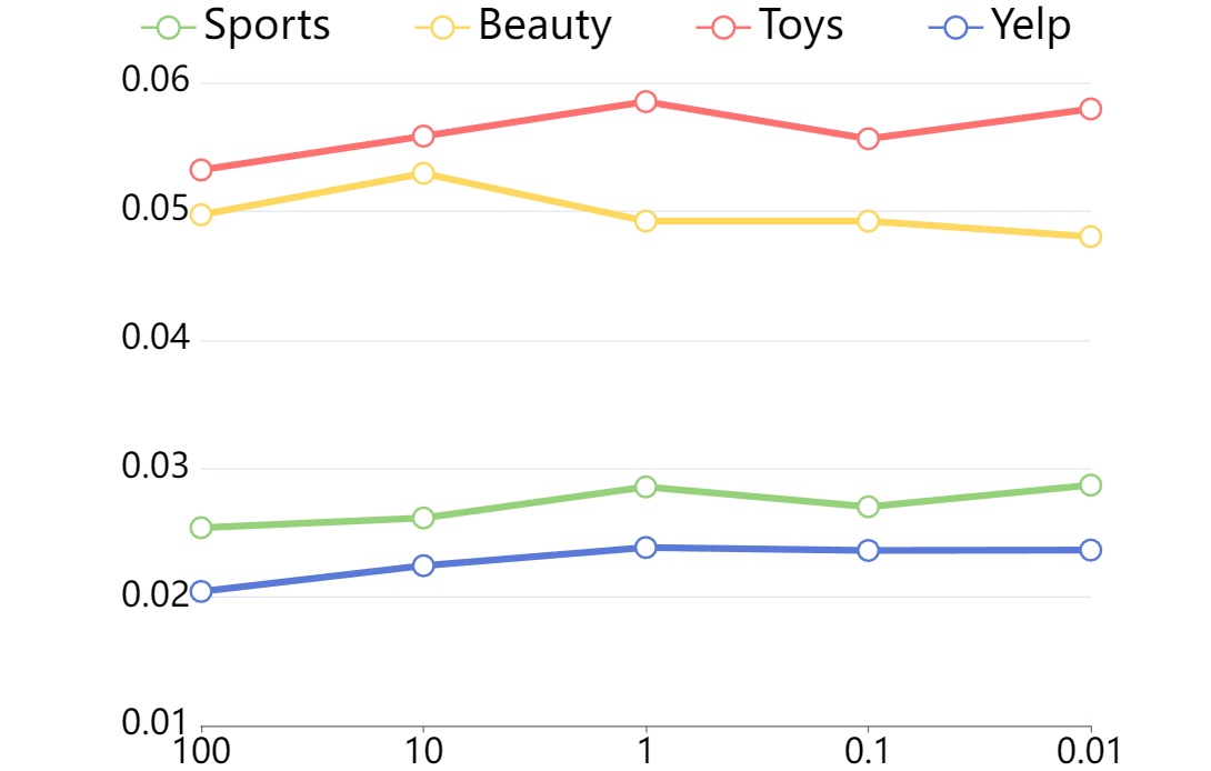
(a) Trade-off $\alpha$

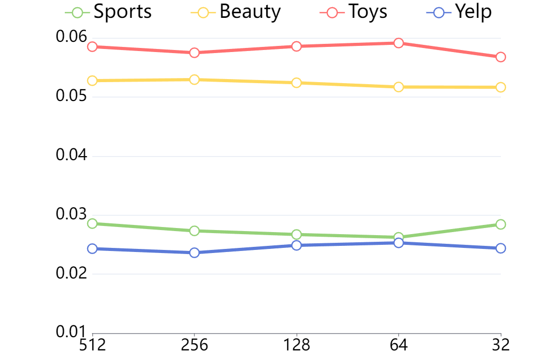
(b) Cluster number $k$

Figure 4: Sensitivity analyses of ELCRec. The results are evaluated by the HR@5 metric.

1. For the trade hyper-parameter $\alpha$, we test the performance with $\alpha\in\{0.01,0.1,1,10,100\}$. We find that our proposed ELCRec is not very sensitive to trade-off $\alpha$. And ELCRec can achieve promising performance when $\alpha\in[0.1,10]$.

2. For the cluster number $k$, we test the recommendation performance with $\alpha\in\{32,64,128,256,512\}$. The results show that ELCRec is also not very sensitive to cluster number $k$ and can perform well when $k\in[256,512]$.

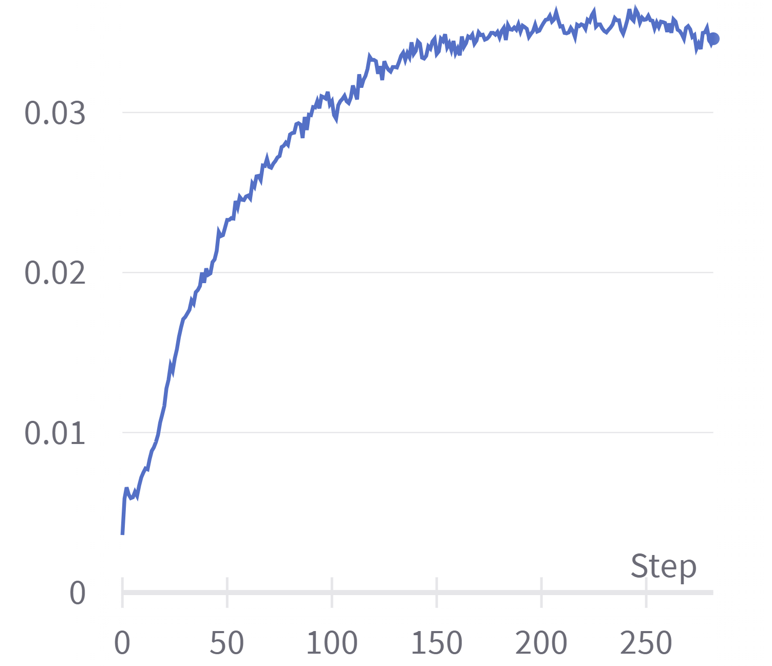
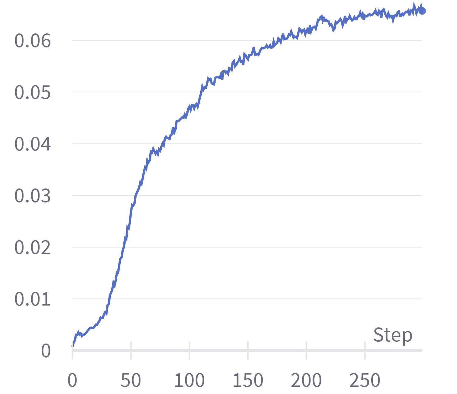
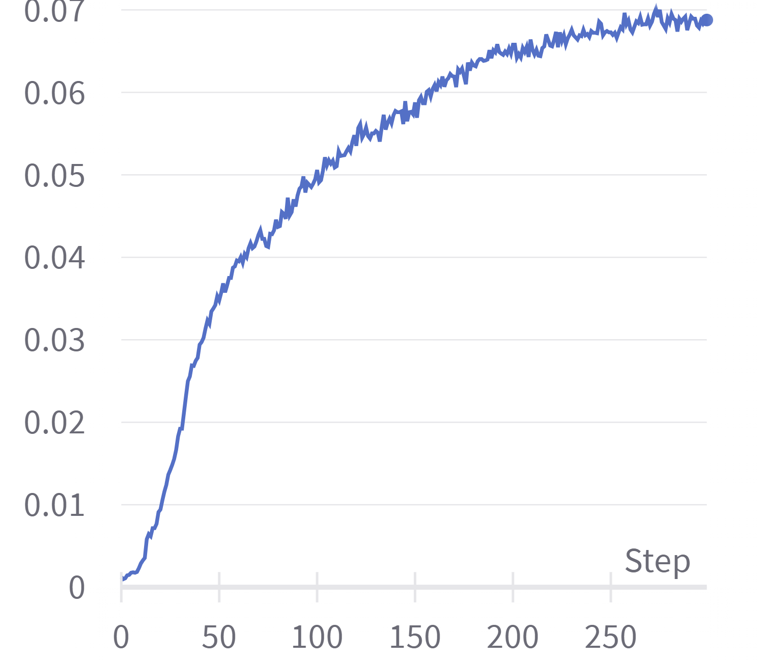
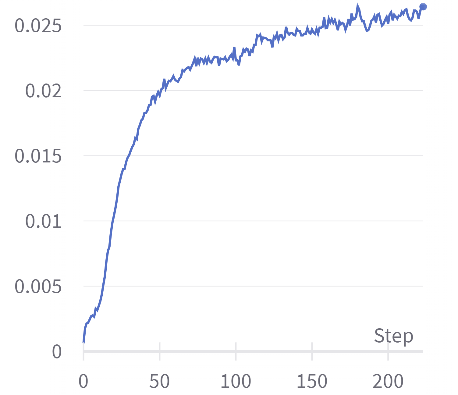
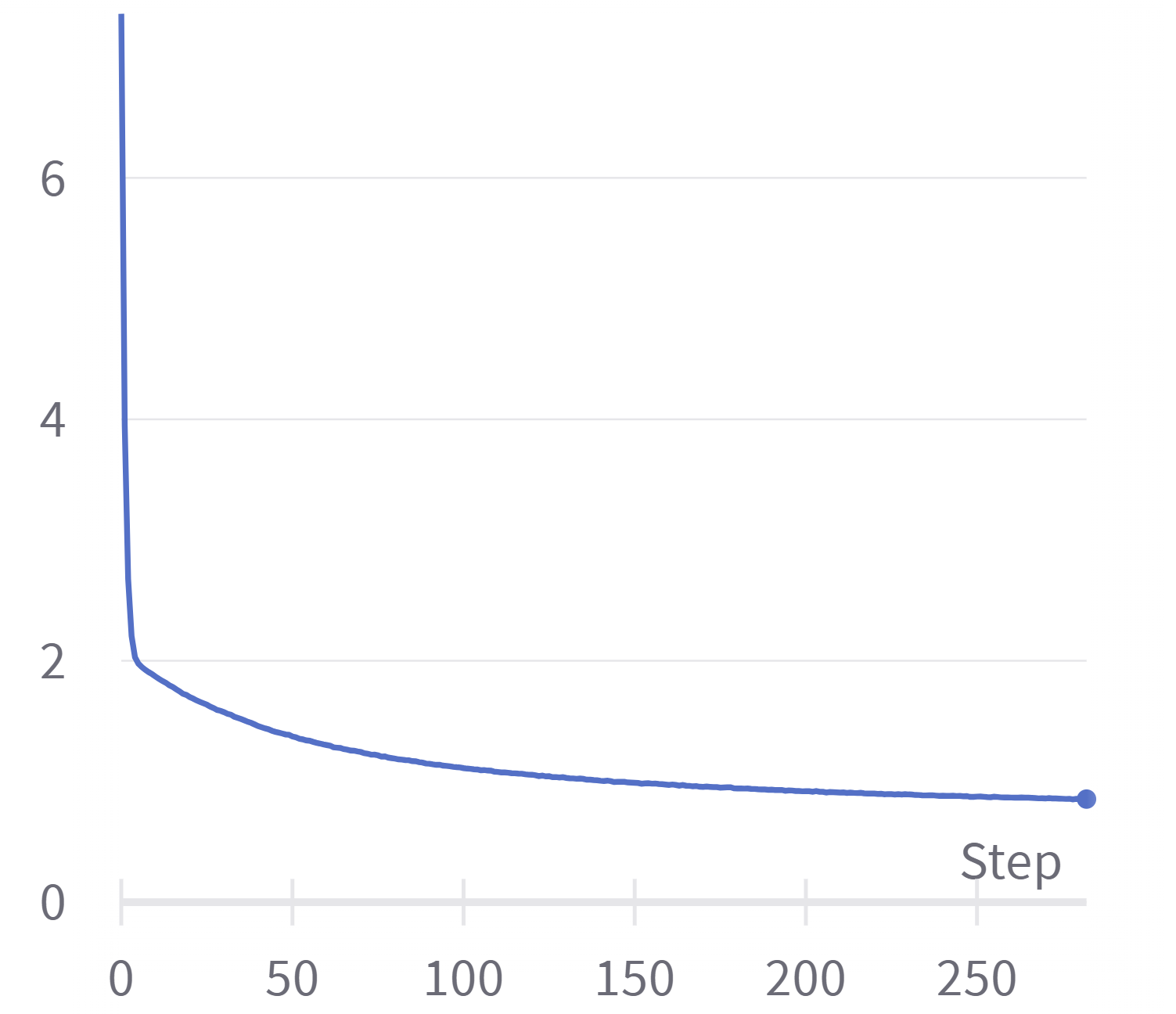
(a) Sports

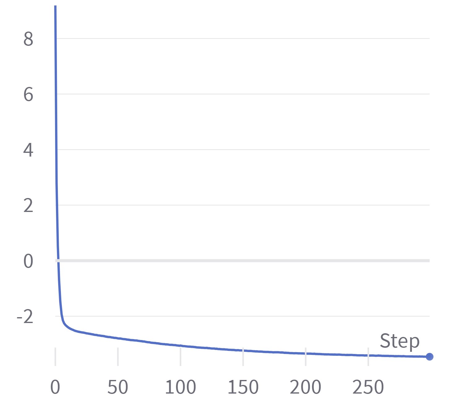
(b) Beauty

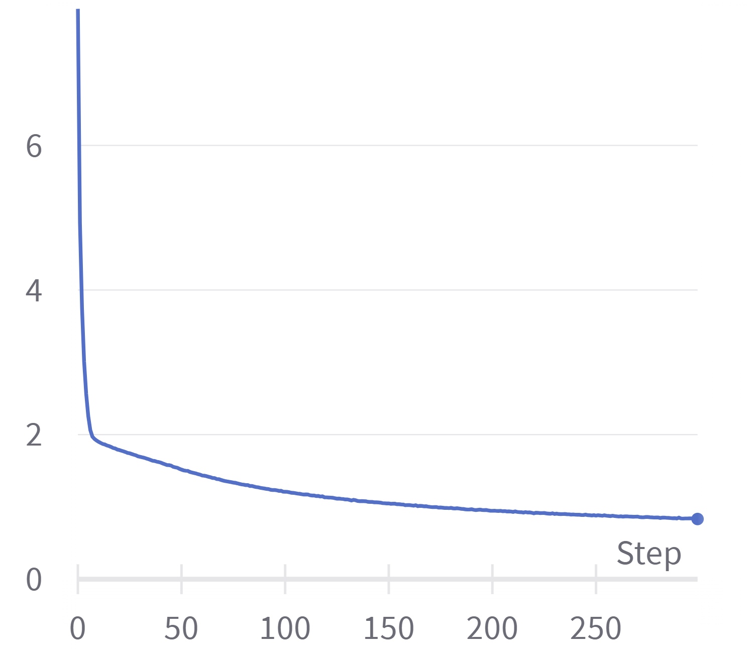
(c) Toys

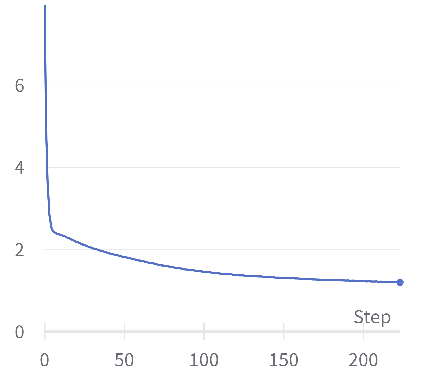
(d) Yelp

Figure 5: Convergence analyses. The first and second row denotes HR@5 on the evaluation set and training loss, respectively.

A.6 Convergence

To answer the research question (v), we monitor the recommendation performance and training loss as shown in Figure 5. We find that the losses gradually decrease and eventually converge. Besides, during the training process, the recommendation performance gradually increases and eventually reaches a promising value.

A.7 Visualization

We conduct visualization experiments on four public datasets to further demonstrate ELCRec’s capability to capture users’ underlying intents. Concretely, the learned behavior embeddings are visualized via $t$-SNE during training. As shown in Figure 6, the first row to the fourth row denotes the results on Sports, Beauty, Toys, and Yelp, respectively. From these experimental results, we have three observations as follows.

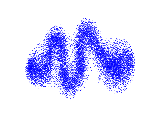
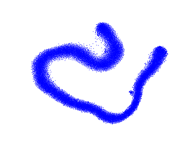
(a) 0 epoch

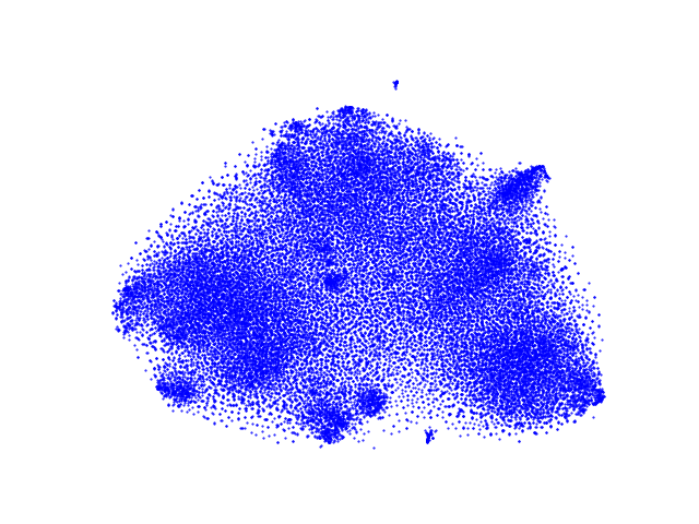
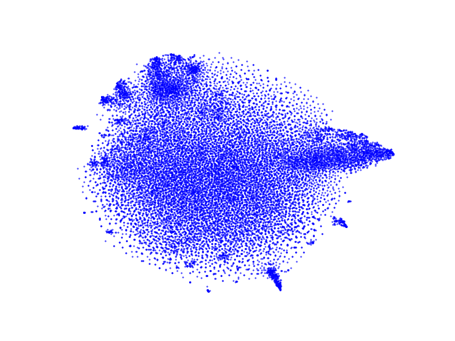
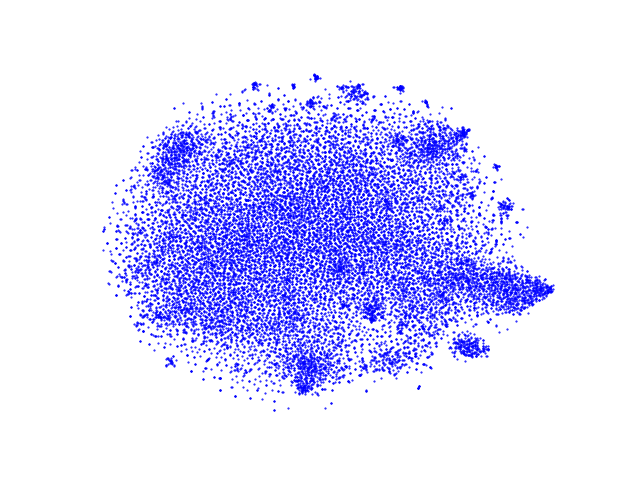
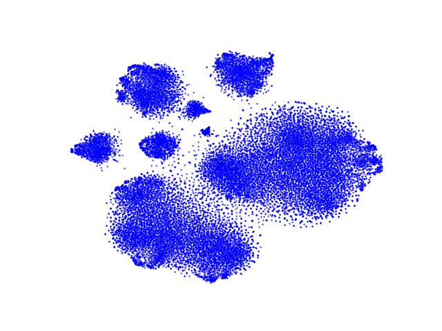
(b) 50 epoch

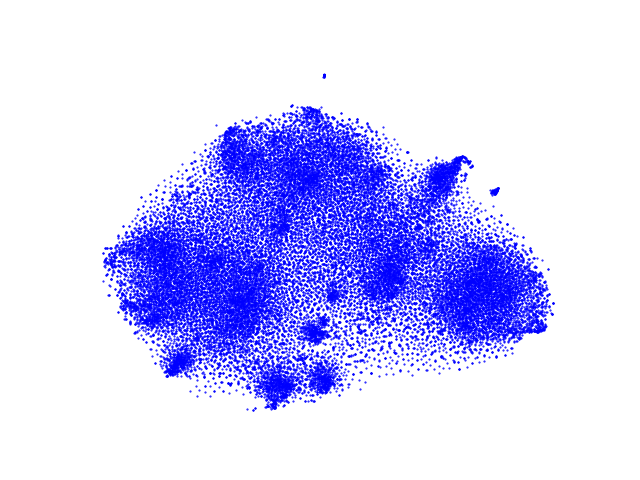
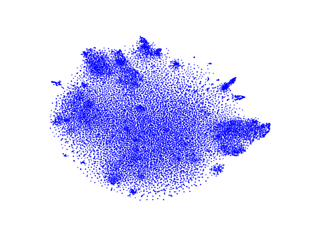
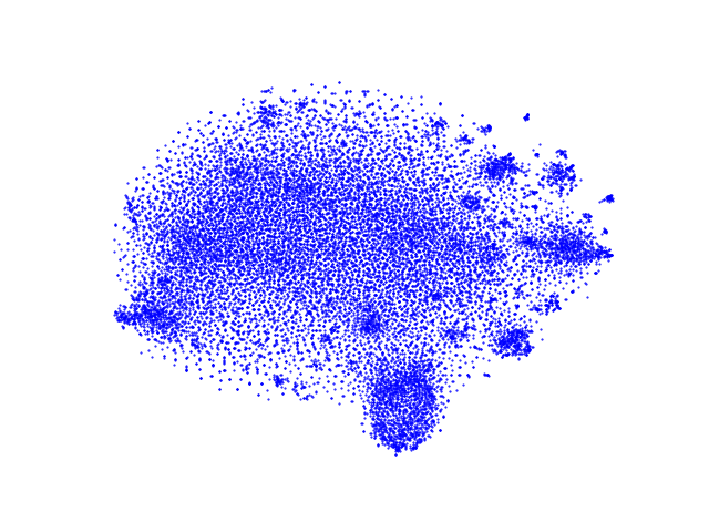
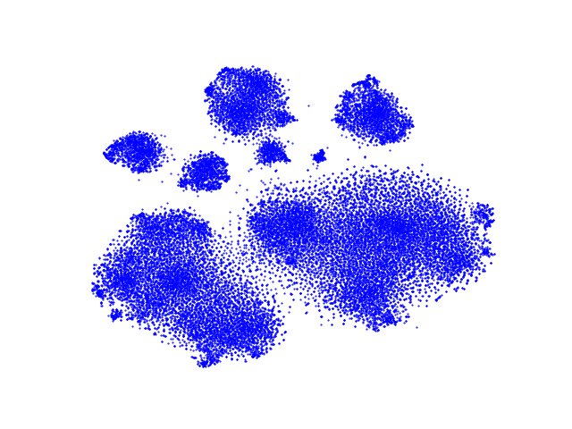
(c) 100 epoch

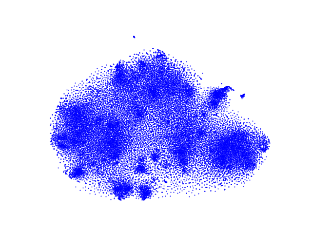
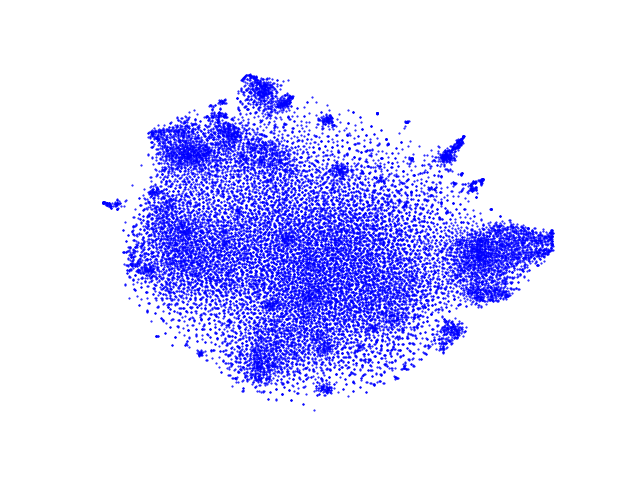
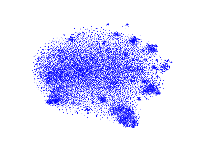
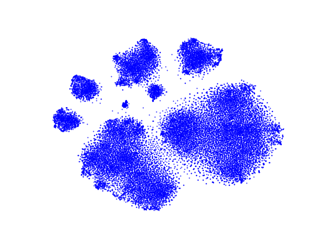
(d) 150 epoch

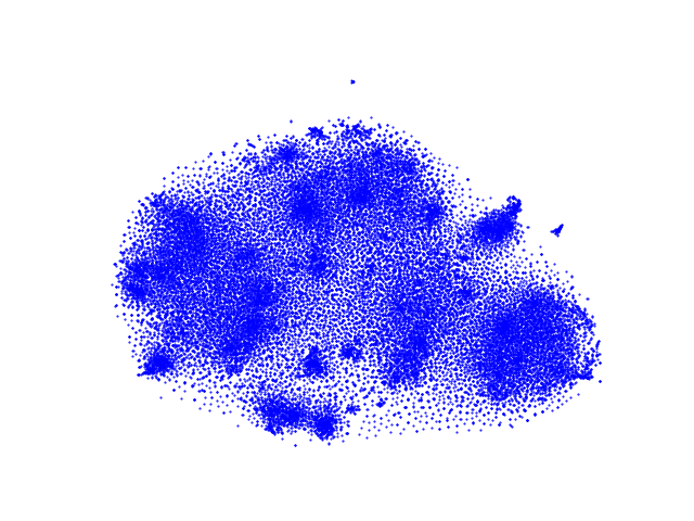
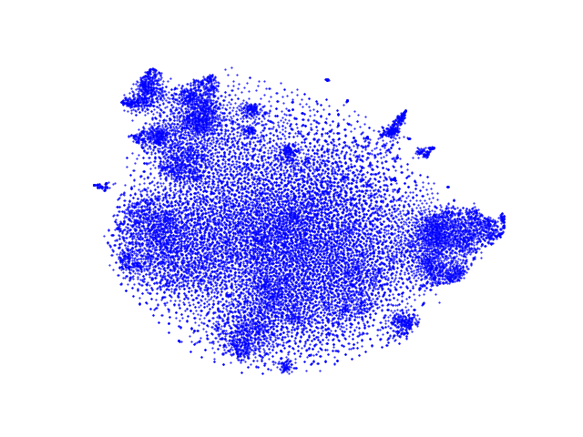
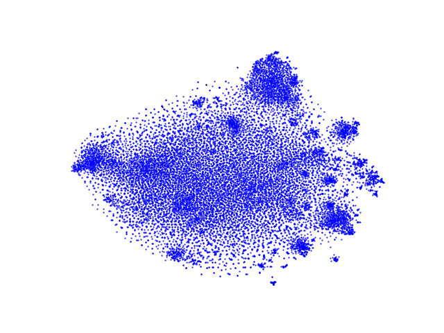
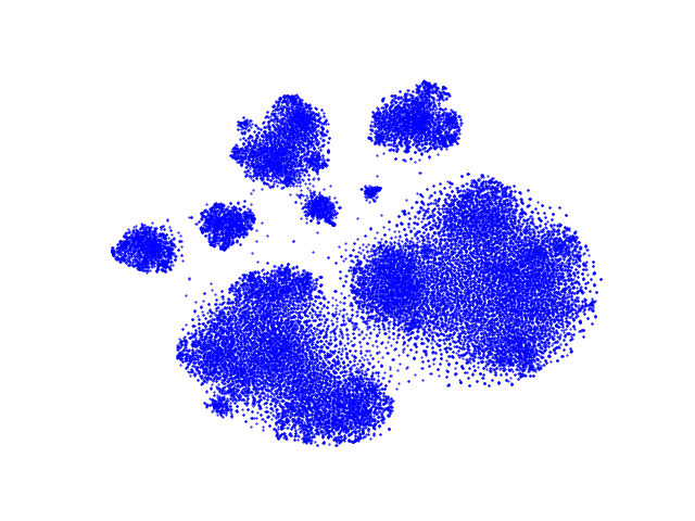
(e) 200 epoch

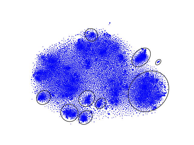
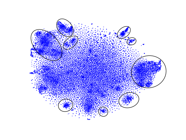
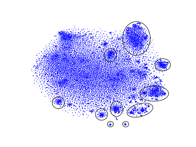
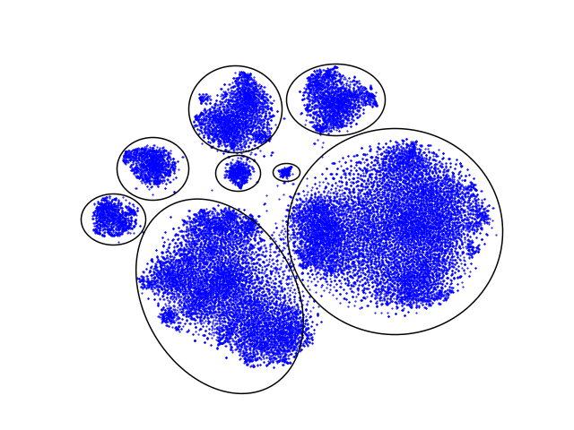
(f) final epoch

Figure 6: t-SNE visualization on four public datasets. The first row to the fourth row denotes the results on Sports, Beauty, Toys, and Yelp.

1. At the beginning of training, the behavior embeddings are disorganized and can not reveal the underlying intents.

2. During the training process, the latent distribution is optimized, and similar behaviors are grouped into latent intents.

3. After optimization, the users’ underlying intents appear, and we highlight them with circles in Figure 6. These intents can assist recommendation systems in better modeling users’ behavior and recommending items. In summary, the above experiments and observations verify the effectiveness of our proposed ELCRec.

A.8 Implementation Details of Baselines

For the baseline methods, we adopt the public source code with the default parameter settings and reproduce their results on the used four benchmarks. The source codes of these methods are available at Table 11. Besides, for the used benchmarks, following (Chen et al., 2022), we only kept datasets where all users and items have at least five interactions. Besides, we adopted the dataset split settings used in (Chen et al., 2022). The Sports, Beauty, and Toys datasets (McAuley et al., 2015; He & McAuley, 2016b) are obtained from: http://jmcauley.ucsd.edu/data/amazon/index.html. The yelp dataset is obtained from https://www.yelp.com/dataset.

Table 11: Implementation URLs of baseline methods.

Method	Url
BPR-MF (Rendle et al., 2012)	https://github.com/xiangwang1223/neural_graph_collaborative_filtering
GRU4Rec (Hidasi et al., 2015)	https://github.com/slientGe/Sequential_Recommendation_Tensorflow
Caser (Tang & Wang, 2018)	https://github.com/graytowne/caser_pytorch
SASRec (Kang & McAuley, 2018)	https://github.com/kang205/SASRec
BERT4Rec (Sun et al., 2019)	https://github.com/FeiSun/BERT4Rec
DSSRec (Ma et al., 2020)	https://github.com/abinashsinha330/DSSRec
S3-Rec (Zhou et al., 2020)	https://github.com/RUCAIBox/CIKM2020-S3Rec
CL4SRec (Xie et al., 2022)	https://github.com/HKUDS/SSLRec
ICLRec (Chen et al., 2022)	https://github.com/salesforce/ICLRec
DCRec (Yang et al., 2023)	https://github.com/HKUDS/DCRec
MAERec (Ye et al., 2023b)	https://github.com/HKUDS/MAERec
IOCRec (Li et al., 2023b)	https://github.com/LFM-bot/IOCRec

A.9 Deployment Details

We aim to apply our proposed method to the real-time large-scale industrial recommendation systems. Concretely, the ELCRec algorithm is applied to livestreaming recommendation in the front page of the Alipay app. The user view (UV) and page view (PV) of this application are about 50 million and 130 million, respectively. Since most of the users are new to this application, it easily leads to the sparsity of users’ behaviors, namely, the cold-start problem in recommendation systems. Our proposed ELCRec can alleviate this problem by grouping users and then making recommendations.

At first, we introduce the online baseline of this project. Since the sparsity of the users’ behaviors, we replaced the users’ behaviors with the users’ activities. Then, the online baseline multi-gate mixture-of-expert (MMOE) (Ma et al., 2018) models the users’ activities. In this model, the experts are designed to extract the features of users, and the multi-gates are designed to select specific experts. The inputs of the multi-gates are the activities of the users. This design aims to train an activity-awarded model to group different users and then conduct recommendations.

However, we found the performance of this model is limited, and the output of the gates is smooth, indicating that this model may fail to group users. Meanwhile, on the open benchmarks, extensive experiments demonstrate the proposed end-to-end learnable clustering module is effective and scalable. Thus, to solve the above problem, ELCRec is adopted in this project. It is designed to assist the gate to group users. For example, the high-activity users and new users are grouped into different clusters, and then the users in different groups will be recommended differently. Therefore, it alleviates the cold-start issue and further improves the recommendation performance. Besides, during the learning process of the cluster embeddings, the low-activity users can transfer to high-activity users, improving the overall users’ activities in the application. It is worth mentioning that the networks are trained with multi-task targets, e.g., CTR prediction, CVR prediction, etc. Following the previous online baseline, the method is implemented with the TensorFlow deep learning platform (Abadi et al., 2016).

A.10 Practical Insights

In this section, we provide practical experiences and insights for the deployment of our proposed method. They contain three parts, including case study, solutions to rapid shift problm, and solutions to balance problem.

A.10.1 Case Study

To explore how our proposed method works well, we conduct case studies on large-scale industrial data. They contain two parts: case studies on user group distribution and case studies on the learned clusters.

Firstly, for the user group distribution, the results are demonstrated in Figure 7. We visualize the cluster distribution of different user groups. “top” denotes the cluster IDs that have the highest proportion in the user group. “bottom” denotes the cluster IDs that have the lowest proportion in the user group. From these analyses, we have two findings as follows.

(a) New users

(b) Low-activity users

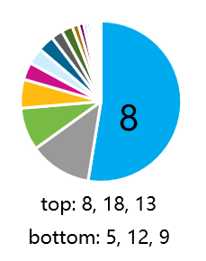
(c) Medium-activity users

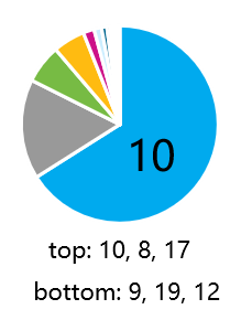
(d) High-activity users

Figure 7: Case studies on different user groups. The distributions of different user groups are visualized. “top” denotes the cluster IDs, which have the highest proportion in the user group. “bottom” denotes the cluster IDs, which have the lowest proportion in the user group.

1. As the user activity increases, the distribution becomes sharper. Namely, the users who have higher activities tend to distribute to one or two clusters. For example, about 60% of the high-activity users are attributed to cluster 10.

2. The “top” cluster IDs of the high-activity user group, such as cluster 10 and cluster 8, are exactly the “bottom” cluster IDs of the low-activity user group. Similarly, the “bottom” cluster IDs of the high-activity user group, such as cluster 9, are exactly the “top” cluster IDs of the low-activity user group. This indicates that the learned cluster centers can well separate different user groups.

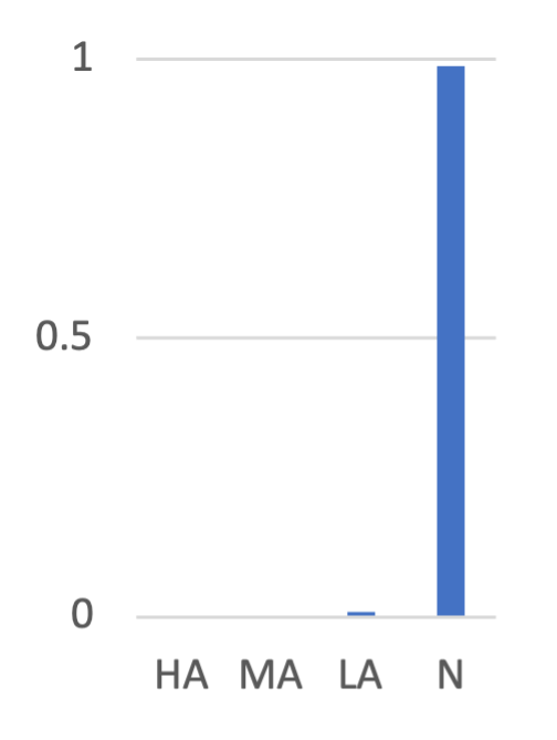
(a) Cluster 6

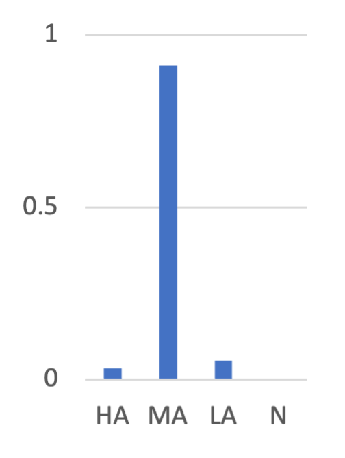
(b) Cluster 8

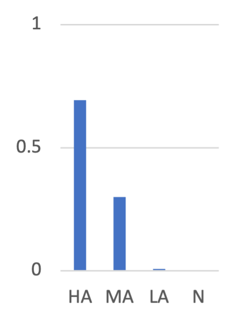
(c) Cluster 10

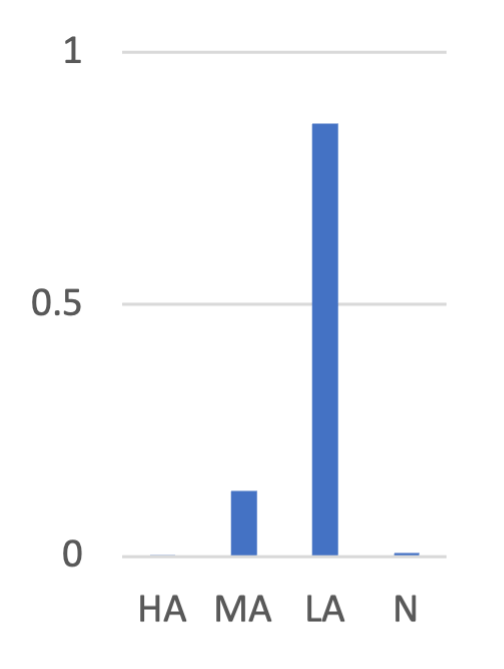
(d) Cluster 13

Figure 8: Case studies on the learned cluster. We visualize the distribution of the learned clusters. “HA”, “MA”, “LA”, and “N” denotes the high-activity, medium-activity, low-activity, and new user groups, respectively.

Secondly, we also conduct extensive case studies on the learned clusters. To be specific, we analyze the user distribution of each cluster, as shown in Figure 8. From the results, we can observe that, in cluster 6, most users are new. Besides, in the cluster 8, the most users are with medium activity. In addition, in cluster 10, most users are with high activity and medium activity. Moreover, in cluster 13, most users are with low activity and medium activity. Previous observations show that the learned centers can separate the users into different groups based on their activities.

In summary, these case studies further verify the effectiveness of ELCRec. Also, they provide insights for future work.

A.10.2 Solutions to Rapid Shift Problem

On real-time large-scale industrial data, the users’ behaviors and intents will shift rapidly. Therefore, we argue that the existing EM optimization can not capture the latest users’ intents, thus easily misunderstanding users and harming recommendation performance. Fortunately, our proposed ELCRec method can alleviate this problem. Concretely, the end-to-end learnable cluster module can guide the network to learn users’ intents dynamically. It can update the learned clusters (intents) at each batch, satisfying the requirement of rapid update. However, our method is hard to control the update rate of the users’ intents. That is one of drawbacks of ELCRec, we will discuses it and the potential solution in A.11.

A.10.3 Solutions to Balance Problem

Balancing the different loss functions in our model is indeed an important challenge. Our overall loss function consists of next-item prediction loss, intent-assisted contrastive loss, and cluster loss. It is formulated as follows: $\mathcal{L}_{\text{overall}}=\mathcal{L}_{\text{next\_item}}+0.1\times\mathcal{L}_{\text{icl}}+\alpha\times\mathcal{L}_{\text{cluster}}$. We set the weight of $\mathcal{L}_{\text{icl}}$ as 0.1 to maintain it in the same order of magnitude as the first term. This reduces the number of hyper-parameters and simplifies the selection process. The weight of $\mathcal{L}_{\text{cluster}}$ is set as a hyper-parameter $\alpha$. We test different values of $\alpha\in\{0.01,0.1,1,10,100\}$ and find that our ELCRec method is not very sensitive to the trade-off $\alpha$. Promising performance is achieved when $\alpha\in[0.1,10]$. The sensitivity analysis experiments are presented in Figure 4 (b). In our proposed model, we set $\alpha$ to 1 for the Sports and Toys datasets, 0.1 for the Yelp dataset, and 10 for the Beauty dataset. The selection of $\alpha$ is mainly based on the model performance. We provide several practical strategies to balance multiple losses in multi-task learning.

• Weighted Balancing. Assign weights to each loss function to control their contribution to the overall loss. By adjusting the weights, a balance can be achieved between different loss functions. This can be determined through prior knowledge, empirical rules, or methods like cross-validation.

• Dynamic Weight Adjustment. Adjust the weights of the loss functions in real time based on the model’s training progress or the characteristics of the data. For example, dynamically adjust the weights based on the model’s performance on a validation set, giving relatively smaller weights to underperforming loss functions.

• Multi-objective Optimization. Treat different loss functions as multiple optimization objectives and use multi-objective optimization algorithms to balance these objectives. This allows for the simultaneous optimization of multiple loss functions and seeks balance between them.

• Gradient-based Adaptive Adjustment. Adaptively adjust the weights of loss functions based on their gradients. If a loss function has a larger gradient, it may have a greater impact on the model’s training, and its weight can be increased accordingly.

• Ensemble Methods. Train multiple models based on different loss functions and use ensemble learning techniques to combine their prediction results. By combining the predictions of different models, a balance between different loss functions can be achieved.

In the future, we will continue to improve our model based the above strategies.

A.11 Limitations & Future Work

In this paper, we propose a novel intent learning method named ELCRec based on the end-to-end learnable clustering framework. It can better mine users’ underlying intents via unifying representation learning and clustering optimization. Besides, the end-to-end learnable clustering module optimizes the clustering distribution via mini-batch data, thus improving the scalability and convenience of deployment. Moreover, we demonstrate the superiority, effectiveness, efficiency, sensitivity, convergence, and visualization of ELCRec on four benchmarks. ELCRec is also successfully applied in the real-time large-scale industrial recommendation system. Although achieving promising results, we admit the proposed ELCRec algorithm has several limitations and drawbacks. We summarize them as follows.

• Pre-defined Cluster Number. The cluster number in ELCRec is a pre-defined hyper-parameter. In the real-time large scale data, it is hard to determine the cluster number, especially under the unsupervised conditions. In this paper, for the open benchmarks, we search the cluster number in {32, 64, 128, 256, 512}. Besides, for the industrial application, the cluster number is set to 20 based on the number of user groups. However, either the search method or the expert knowledge can not determine the cluster number well at once. The cluster number may change dynamically during model training, and the proposed method may fail to achieve promising performance.

• Limited Recommendation Domains. In this paper, we adopt four recommendation benchmarks, including Sports, Beauty, Toys, and Yelp, for the main experimental results. But, these four datasets are all buying recommendation datasets. Besides, we adopt ML-1M (Harper & Konstan, 2015) and MIND-small (Wu et al., 2020) for the movie and news recommendation for the additional experiments. However, the recommendation domains are still limited. In the future, we can further demonstrate the boarder applicability of ELCRec in other domains.

• Uncontrollable Update Rate of Cluster Centers. In the real-time recommendation system, the users’ behaviors and intents usually change rapidly. Although our proposed ELCRec can dynamically learn the users’ intents, it is hard to control the update rate of the underlying clusters (intents).

To solve these issues, we summarize several future works and the potential technical solutions as follows.

• Density-based Clustering. As mentioned above, the cluster number is a pre-defined value in this paper, limiting the recommendation performance and flexibility of the method. To solve this issue in the future, firstly, we can determine the cluster number based on some cluster number estimation methods. They can help to determine the cluster number by performing multiple clustering runs and selecting the best cluster number based on the unsupervised criterion. The mainstream cluster number estimation methods (Kodinariya et al., 2013) include the thumb rule, ELBOW (Syakur et al., 2018), $t$-SNE (Van der Maaten & Hinton, 2008), etc. The thumb rule simply assigns the cluster number $k$ with $\sqrt{n/2}$, where $n$ is the number of samples. This manual setting is empirical and can not be applicable to all datasets. Besides, the ELBOW is a visual method. Concretely, they start the cluster number $k=2$ and keep increasing $k$ in each step by 1, calculating the WSS (within-cluster sum of squares) during training. They choose the value of $k$ when the WSS drops dramatically, and after that, it reaches a plateau. However, it will bring large computational costs since the deep neural network needs to be trained with repeated times. Another visual method termed $t$-SNE visualizes the high-dimension data into 2D sample points and helps researchers determine the cluster number. The effectiveness of $t$-SNE heavily relies on the experience of researchers. Therefore, secondly, we can determine the cluster number based on the data density (Rodriguez & Laio, 2014; Ronen et al., 2022). Concretely, the areas with high data density are identified as the cluster centers, while the areas with low data density are identified as the decision boundaries between cluster centers. Besides reinforcement learning is also a potential solution (Liu et al., 2023a). Through these designs, the cluster number will be changeable during the training process. It will be determined based on the embeddings itself, better revealing the users’ behavior and may achieve better recommendation performance.

• More Recommendation Domains. As mentioned above, the applied recommendation domains of our method are limited. We aim to test ELCRec on more recommendation domains, such as music recommendation (Zhang et al., 2022a; Brost et al., 2019), group recommendation (Zhang et al., 2023a; Liu et al., 2022a), group buying (Zhai et al., 2023), bundle recommendation (Zou et al., 2023), etc.

• Controllable Intent Learning. As mentioned above, in the real-time recommendation system, the intents of the users may change rapidly. Our method makes it hard to control the intent update rate during training and inference. To this end, in the future, we can propose a controllable cluster center learning method, such as the momentum update, to control the change rate of the users’ intents. Concretely, $\mathbf{C}_{t}=m\cdot\mathbf{C}_{t}+(1-m)\cdot\mathbf{C}_{t-1}$. Here, $\mathbf{C}_{t}$ denote the cluster center embeddings at $t$ and $m$ denotes the momentum. Then, the cluster centers (intents of users) will be changed rapidly when $m$ is large, and the cluster centers (intents of users) will be changed slowly when $m$ is small. This strategy will control the change rate of the users’ intent embeddings, therefore alleviating the above problem.

References

- Abadi et al. (2016) Abadi, M., Barham, P., Chen, J., Chen, Z., Davis, A., Dean, J., Devin, M., Ghemawat, S., Irving, G., Isard, M., et al. TensorFlow: a system for Large-Scale machine learning. In 12th USENIX symposium on operating systems design and implementation (OSDI 16), pp. 265–283, 2016.
- Aggarwal & Zhai (2012) Aggarwal, C. C. and Zhai, C. A survey of text clustering algorithms. Mining text data, pp. 77–128, 2012.
- Asano et al. (2019) Asano, Y., Rupprecht, C., and Vedaldi, A. Self-labelling via simultaneous clustering and representation learning. In International Conference on Learning Representations, 2019.
- Bai et al. (2024) Bai, Y., Zhou, Y., Dou, Z., and Wen, J.-R. Intent-oriented dynamic interest modeling for personalized web search. ACM Transactions on Information Systems, 2024.