A $k$-swap Local Search for Makespan Scheduling

Abstract

Local search is a widely used technique for tackling challenging optimization problems, offering significant advantages in terms of computational efficiency and exhibiting strong empirical behavior across a wide range of problem domains. In this paper, we address a scheduling problem on two identical parallel machines with the objective of makespan minimization. For this problem, we consider a local search neighborhood, called $k$-swap, which is a more generalized version of the widely-used swap and jump neighborhoods. The $k$-swap neighborhood is obtained by swapping at most $k$ jobs between two machines in our schedule. First, we propose an algorithm for finding an improving neighbor in the $k$-swap neighborhood which is faster than the naive approach, and prove an almost matching lower bound on any such an algorithm. Then, we analyze the number of local search steps required to converge to a local optimum with respect to the $k$-swap neighborhood. For the case $k=2$ (similar to the swap neighborhood), we provide a polynomial upper bound on the number of local search steps, and for the case $k=3$, we provide an exponential lower bound. Finally, we conduct computational experiments on various families of instances, and we discuss extensions to more than two machines in our schedule.

Keywords: Local Search, Scheduling, Makespan Minimization, $k$-swap

1 Introduction

Local search methods are some of the most widely used heuristics for approaching computationally difficult optimization problems [1, 25]. Their appeal comes not only from their simplicity but also from their good empirical behavior as shown, for instance, by the 2-opt neighborhood [1, 10, 13] for the traveling salesman problem (TSP). The local search procedure starts with an initial solution and iteratively moves from a feasible solution to a neighboring solution until specific stopping criteria are satisfied. The performance of local search is significantly impacted by the selection of an appropriate neighborhood function. These functions determine the range of solutions that the local search procedure can explore in a single iteration. The most straightforward type of local search, known as iterative improvement, continuously selects a better solution within the neighborhood of the current one. The iterative improvement process stops when no further improvements can be made within the neighborhood, signifying that the procedure has reached a local optimum.

In this paper, we consider one of the most fundamental scheduling problems, in which we are given a set of $n$ jobs, each of which needs to be processed on one of two identical machines without preemption. All the jobs and machines are available from time $0$, and a machine can process at most one job at a time. The objective that we consider is makespan minimization: we want the last job to be completed as early as possible. This problem, denoted by $P2{\parallel}C_{\max}$ [17], may seem straightforward and simple at first glance; however, is known to be NP-hard [21]. Despite the simplicity of this problem at first glance, there is not a comprehensive theoretical understanding of local search algorithms for it, which motivates the study of it in this paper.

Formal model.

As the order in which the jobs, assigned to the same machine, are processed, does not influence the makespan, we represent a schedule by $\sigma=(M_{1},M_{2})$, where $M_{i}$ represents the set of jobs scheduled on machine $i$ (for $i\in\{1,2\}$). Let $L_{i}=\sum_{j\in M_{i}}p_{j}$ denote the load of machine $i$, where $p_{j}$ is the time required to process job $j$. In this setting, the makespan of a schedule, commonly denoted by $C_{\max}$, is equal to the maximum load, i.e., $L_{\max}=\max_{i}L_{i}$, which we want to minimize (we use the notations $C_{\max}$ and $L_{\max}$ interchangeably throughout the paper). The critical machine is the machine whose load is equal to the makespan, and the min-load machine is the machine with a load $L_{\min}=\min_{i}L_{i}$. We define $\Delta=L_{\max}-L_{\min}$, as the difference between the maximum and minimum machine load.

Related work.

One of the simplest neighborhoods for addressing the problem $P2{\parallel}C_{\max}$ is the so-called jump neighborhood, which is also known as the move neighborhood. To obtain a jump neighbor, only the machine allocation of one job changes. Finn and Horowitz [12] have proposed a simple improvement heuristic, called 0/1-Interchange, which is able to find a local optimum with respect to the jump neighborhood. Brucker et al. [7] showed that the 0/1-Interchange algorithm terminates in $O(n^{2})$ steps, regardless of the job selection rule; the tightness of this bound was shown by Hurkens and Vredeveld [20]. The upper bound of $O(n^{2})$ was first obtained for schedules with 2 machines and was extended later to schedules with an arbitrary number of machines [8]. Similarly, the other results in the remainder of this paragraph also hold for an arbitrary number of machines. Another well-known folklore neighborhood is the swap neighborhood. For obtaining a swap neighbor, two jobs, scheduled on different machines, are selected, and the neighbor is obtained by interchanging the machine allocations of these two jobs. Many other neighborhoods, such as push [30], multi-exchange [3, 14] and split [9] have also been proposed in the literature to solve this problem. In addition to local search, various approximation algorithms have been introduced to address scheduling problems. Among them, some of the first approximation algorithms [15, 16] and polynomial time approximation schemes (PTAS) [22] have been developed in the context of scheduling problems. It has been shown that there exists a fully polynomial time approximation scheme (FPTAS) for this problem [29, 31] when the number of machines is a constant $m$ ($Pm||C_{\max}$). When the number of machines is part of the input ($P||C_{\max}$), a PTAS has been provided [18] for this problem, and the best-known running time of such a scheme is proposed by Berndt et al [6]. PTAS’s are often considered impractical due to their tendency to yield excessively high running time bounds (albeit polynomial) even for moderate values of $\varepsilon$ (see [24]). In consequence, we focus on a local search study of the problem $P2||C_{\max}$. Local search methods are studied extensively for various other problems as well. In particular, the $k$-opt heuristic has been proposed for TSP, and has been the subject of theoretical study. For example, de Berg et al. [5] have proposed an algorithm that finds the best $k$-opt move faster than the naive approach.

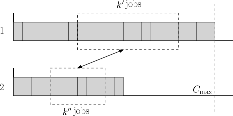
Figure 1: $k$-swap operator.

Our contribution.

In this paper, we consider a generalization of the jump and swap neighborhoods for the problem $P2{\parallel}C_{\max}$, which is called the $k$-swap neighborhood. To obtain a $k$-swap neighbor, we select $k^{\prime}$ jobs from one machine and $k^{\prime\prime}$ jobs from another machine, such that $k^{\prime}+k^{\prime\prime}\leq k$, and then we interchange the machine allocations of these jobs (see Fig. 1). We say we are in a k-swap optimal solution if we cannot decrease the makespan by applying the $k$-swap operator. For $k=1$, the $k$-swap neighborhood is the same as the jump neighborhood, and for $k=2$, the $k$-swap neighborhood contains all possible jumps and swaps. We note that the $k$-swap neighborhood is identical to $k$-move neighborhood (a neighborhood that has been also studied by Dumrauf et al. [11]) when we have only two machines in our schedule. A naive implementation of the $k$-swap takes $O(k\cdot n^{k})$ steps to find an improving neighbor (if it exists). We propose a randomized algorithm for finding an improving solution in the $k$-swap neighborhood in $O(n^{\lceil\frac{k}{2}\rceil+O(1)})$ steps. Then, we show how to derandomize this algorithm. Assuming the $k$-sum conjecture [2], which states for every $k\geq 2$ and $\varepsilon>0$, the $k$-sum problem cannot be solved in $O(n^{\lceil k/2\rceil-\varepsilon})$ (randomized) time, we show that the proposed randomized algorithm is almost tight by establishing a lower bound of $O(n^{\lceil k/2\rceil})$ for the problem of finding an improving neighbor in the $k$-swap neighborhood. We complement these results by providing an upper bound of $O(n^{4})$ on the number of local search steps required to converge to a local optimum for $k=2$, and providing an exponential lower bound for the case where we swap exactly three jobs in each step. Additionally, we have conducted computational experiments on various families of instances to compare the efficiency of our proposed randomized algorithm against the naive approach of searching the $k$-swap neighborhood.

2 Searching the Neighborhood

In order to find an improving $k$-swap neighbor, we need to find a set $S_{k^{\prime}}$ of $k^{\prime}$ jobs from the critical machine $1$ and a set $S_{k^{\prime\prime}}$ of $k^{\prime\prime}$ jobs from the min-load machine $2$ such that $0<\sum_{j\in S_{k^{\prime}}}p_{j}-\sum_{j\in S_{k^{\prime\prime}}}p_{j}<\Delta$ and $k^{\prime}+k^{\prime\prime}\leq k$. In this section, we present an algorithm for finding a better solution in the $k$-swap neighborhood, which is able to find such a solution faster than the naive approach. In a naive approach, we consider swapping all different combinations of at most $k$ jobs with each other. As we have $n$ jobs in our schedule, we need to search over all $O(n^{k})$ different combinations in the worst case to find an improvement (if it exists). In our algorithm, we consider all combinations of at most $\frac{k}{2}$ jobs and then, combine two such combinations to one $k$-swap. This principle is known as the meet-in-the-middle approach [19]. The proposed algorithm is a randomized Monte Carlo algorithm with one-sided error [26]. More precisely, when this algorithm outputs a better solution in the $k$-swap neighborhood, this solution is always correct. Conversely, if the algorithm does not find an improvement, there is a nonzero probability that there exists an improvement.

For the sake of simplicity, we consider swapping exactly $k$ jobs with each other. We can run the proposed algorithm $k-1$ more times for the case of swapping less than $k$ jobs. In this algorithm, first, we divide the set of jobs into two sets $A$ and $B$ uniformly at random. Assume w.l.o.g. that machine 1 is the critical machine. We compute $\sum_{j\in S_{1}\cap M_{1}}p_{j}-\sum_{j\in S_{1}\cap M_{2}}p_{j}$, for all $S_{1}\subseteq A$ with $|S_{1}|=\lceil\frac{k}{2}\rceil$, and we add all the computed values to a set $A_{\Sigma}$. Then, we compute $\sum_{j\in S_{2}\cap M_{1}}p_{j}-\sum_{j\in S_{2}\cap M_{2}}p_{j}$, for all $S_{2}\subseteq B$ with $|S_{2}|=\lfloor\frac{k}{2}\rfloor$, and we add the all the computed values to a set $B_{\Sigma}$. The sets $A_{\Sigma}$ and $B_{\Sigma}$ contain $O(n^{\lceil\frac{k}{2}\rceil})$ numbers as well as references to the corresponding jobs for each number. For simplicity, we treat these sets as sets of numbers. In the next step, we sort the values in the set $B_{\Sigma}$ in non-decreasing order. Then, we need to find some $x\in A_{\Sigma}$ and $y\in B_{\Sigma}$ such that $0<x+y<\Delta$. To this end, for every $x\in A_{\Sigma}$, we search for some $y$ in the sorted list of the values in $B_{\Sigma}$, such that $y\in(-x,\Delta-x)$. This can be implemented by binary search. Our algorithm is described more formally in Algorithm 1.

Algorithm 1 Randomized $k$-swap

1:A schedule $\sigma=(M_{1},M_{2})$ and a value $k$.

2:A Boolean variable, {True, False}, which indicates whether $\sigma$ has been improved or not.

3:Initialize $A=B=A_{\Sigma}=B_{\Sigma}=\varnothing$

4:for each $j\in M_{1}\cup M_{2}$ do

5:     Assign $j$ uniformly at random to $A$ or $B$

6:for each $S_{1}\subseteq A\;\text{with}\;\lvert S_{1}\rvert=\lceil\frac{k}{2}\rceil$ do

7:     $v=\sum_{j\in S_{1}\cap M_{1}}p_{j}-\sum_{j\in S_{1}\cap M_{2}}p_{j}$

8:     $A_{\Sigma}=A_{\Sigma}\cup\{v\}$

9:for each $S_{2}\subseteq B\;\text{with}\;\lvert S_{2}\rvert=\lfloor\frac{k}{2}\rfloor$ do

10:     $v=\sum_{j\in S_{2}\cap M_{1}}p_{j}-\sum_{j\in S_{2}\cap M_{2}}p_{j}$

11:     $B_{\Sigma}=B_{\Sigma}\cup\{v\}$

12:Sort the values in $B_{\Sigma}$ in non-decreasing order

13:for each $x\in A_{\Sigma}$ do

14:     if $B_{\Sigma}$ contains a value $y\in(-x,\Delta-x)$ then

15:         Update $\sigma$ by swapping the corresponding jobs to $x$ $\&$ $y$

16:         return True      

17:return False

Suppose that there are $k$ jobs such that we are able to improve the schedule by swapping them. The above algorithm fails if it does not improve the schedule. Conversely, this algorithm is successful if it manages to improve the schedule by swapping $k$ jobs. It is easy to see that this algorithm is successful if $\lceil\frac{k}{2}\rceil$ of these jobs are in the set $A$ and the remaining are in the set $B$. The probability of success is at least $\dfrac{\binom{k}{\lceil\frac{k}{2}\rceil}}{2^{k}}$ since we assign each job independently at random with equal probability to one of the sets $A$ and $B$. If there is a possibility of improving the schedule by swapping $k$ jobs, there are at least $\binom{k}{\lceil\frac{k}{2}\rceil}$ different ways of assigning $\lceil\frac{k}{2}\rceil$ jobs to the set $A$ and assigning the remaining jobs to the set $B$. Moreover, the probability of failure of the algorithm is at most $1-\dfrac{\binom{k}{\lceil\frac{k}{2}\rceil}}{2^{k}}$. To ensure that we get a constant probability of success, we run the algorithm $\dfrac{2^{k}}{\binom{k}{\lceil\frac{k}{2}\rceil}}$ times.

Lemma 2.1.

If we repeat the randomized k-swap algorithm $\dfrac{2^{k}}{\binom{k}{\lceil\frac{k}{2}\rceil}}$ times, the probability of failure in finding an improving schedule becomes at most $\frac{1}{e}$.

Proof.

The probability of failure of the randomized $k$-swap algorithm is upper-bounded by $1-\dfrac{\binom{k}{\lceil\frac{k}{2}\rceil}}{2^{k}}$ if we run the algorithm only once. If we repeat the algorithm $\gamma=\dfrac{2^{k}}{\binom{k}{\lceil\frac{k}{2}\rceil}}$ times, we get

$$\text{I\kern-1.49994ptP}[\mathrm{failure}]\leq(1-\frac{1}{\gamma})^{\gamma}\leq(e^{-\frac{1}{\gamma}})^{\gamma}=\dfrac{1}{e}.\qed$$

2.1 Running Time

In this part, we analyze the running time of the proposed randomized $k$-swap algorithm.

Lemma 2.2.

The randomized k-swap algorithm terminates in $O(k\cdot n^{\lceil\frac{k}{2}\rceil}\cdot\log n)$ steps.

Proof.

In this algorithm, first, we divide the set of jobs into two sets $A$ and $B$, which take $O(n)$. Then, we create the sets $A_{\Sigma}$ and $B_{\Sigma}$, which takes $O(\lceil\frac{k}{2}\rceil\cdot n^{\lceil\frac{k}{2}\rceil})$ as each set contains $O(n^{\lceil\frac{k}{2}\rceil})$ different numbers, each of which takes $O(\lceil\frac{k}{2}\rceil)$ time to be computed. Then, we sort the numbers in $B_{\Sigma}$ in non-decreasing order, which takes $O(k\cdot n^{\lceil\frac{k}{2}\rceil}\cdot\log n)$. Finally, for every $x\in A_{\Sigma}$, we search for a $y$ in the sorted list of the values in $B_{\Sigma}$, such that $y\in(-x,\Delta-x)$, which also takes $O(k\cdot n^{\lceil\frac{k}{2}\rceil}\cdot\log n)$. ∎

As we stated in Lemma 2.1, we need to repeat the randomized $k$-swap algorithm $\dfrac{2^{k}}{\binom{k}{\lceil\frac{k}{2}\rceil}}$ times to increase the probability of success of the algorithm. Based on the following lemma, we are able to analyze the value $\dfrac{2^{k}}{\binom{k}{\lceil\frac{k}{2}\rceil}}$ asymptotically.

Lemma 2.3.

we have $\binom{k}{\lceil\frac{k}{2}\rceil}=\Theta\left(\dfrac{2^{k}}{\sqrt{k}}\right)$.

Proof.

According to the asymptotic growth of the $n$th central binomial coefficient [23], which states $\binom{2n}{n}=\Theta\left(\dfrac{4^{n}}{\sqrt{\pi n}}\right)$, we get

$$\binom{k}{\lceil\frac{k}{2}\rceil}=\binom{k}{\lfloor\frac{k}{2}\rfloor}=\Theta\binom{2\lfloor\frac{k}{2}\rfloor}{\lfloor\frac{k}{2}\rfloor}=\Theta\left(\frac{4^{\lfloor\frac{k}{2}\rfloor}}{\sqrt{\pi\lfloor\frac{k}{2}\rfloor}}\right)=\Theta\left(\frac{2^{k}}{\sqrt{k}}\right).\qed$$

According to Lemma 2.2, the time complexity of the randomized $k$-swap algorithm is $O(k\cdot n^{\lceil\frac{k}{2}\rceil}\cdot\log n)$. Note that in this algorithm, we have considered swapping exactly $k$ jobs with each other. However, for obtaining a $k$-swap neighbor, we swap at most $k$ jobs with each other. Therefore, for obtaining an improving $k$-swap neighbor, we repeat the randomized $k$-swap algorithm for different values of $k$. As we have

$$k\cdot\log n\cdot n^{\frac{k}{2}}+(k-1)\cdot\log n\cdot n^{\frac{k-1}{2}}+\dotsc+1\cdot\log n\cdot n^{\frac{1}{2}}\leq k\cdot\log n\cdot(n^{\frac{k}{2}}+n^{\frac{k-1}{2}}+\dotsc+n^{\frac{1}{2}}),$$

and $n^{\frac{k}{2}}+n^{\frac{k-1}{2}}+\dotsc+n^{\frac{1}{2}}=O(n^{\frac{k}{2}})$, the time complexity of finding a $k$-swap neighbor remains $O(k\cdot n^{\lceil\frac{k}{2}\rceil}\cdot\log n)$. Furthermore, according to Lemma 2.1 and Lemma 2.3, we need to repeat this algorithm $O(\sqrt{k})$ times to increase the probability of success. Thus, we have the following theorem.

Theorem 2.4.

We are able to find a better solution in the k-swap neighborhood with the probability of success of at least $1-\frac{1}{e}$ in $O(k^{3/2}\cdot n^{\lceil\frac{k}{2}\rceil}\cdot\log n)$ by running the randomized k-swap algorithm $O(\sqrt{k})$ times for different values of $k$.

2.2 Derandomization

In this subsection, we describe a method for derandomizing the randomized $k$-swap algorithm. This method is based on a combinatorial structure called splitters which was introduced by Naor et al. [27] to derandomize the color coding technique, introduced by Alon et al. [4]. Formally, an ($n,k,l$)-splitter is a family of hash functions $H$ from $\{1,...,n\}$ to $\{1,...,l\}$ such that for all $S\subseteq\{1,...,n\}$ with $|S|=k$, there exists a function $h\in H$ that splits $S$ evenly; i.e., for every $j,j^{\prime}\in\{1,...,l\}$, $|h^{-1}(j)\cap S|$ and $|h^{-1}(j^{\prime})\cap S|$ differ by at most 1. It has been shown [4, 27] that there exists an ($n,k,k^{2}$)-splitter of size $k^{6}\cdot\log k\cdot\log n$ which is computable in time complexity of $O(k^{6}\cdot\log k\cdot n\cdot\log n)$.

In our randomized algorithm, we divide the set of jobs uniformly at random into two sets $A$ and $B$. If there exists a set of $k$ jobs such that by swapping them we are able to improve the schedule, the algorithm is successful if $\lceil\frac{k}{2}\rceil$ of these jobs are in the set $A$ and the remaining are in the set $B$. In the derandomized version of this algorithm, instead of dividing the set of jobs uniformly at random into two sets $A$ and $B$, we divide the set of jobs in several different ways based on the functions in an ($n,k,k^{2}$)-splitter. We will show that based on at least one of the functions, $\lceil\frac{k}{2}\rceil$ of the jobs, for which we are looking, will be assigned to the set $A$, and the remaining will be assigned to the set $B$. The idea of how to derandomize our algorithm is explained in more detail below.

If we map each of the jobs to a number $\{c_{1},c_{2},...,c_{k^{2}}\}$ based on the functions in an ($n,k,k^{2}$)-splitter, according to at least one of these functions, those $k$ jobs, for which we are looking, will be mapped to different numbers. As we want $\lceil\frac{k}{2}\rceil$ of these $k$ jobs to be assigned to the set $A$ and the remaining to be assigned to the set $B$, we map the numbers $\{c_{1},c_{2},...,c_{k^{2}}\}$ to only two numbers 0 and 1, and then, we say those jobs which are mapped to 0 are in the set $A$ and the jobs which are mapped to 1 are in the set $B$ (or vice versa). To make sure that after mapping the numbers $\{c_{1},c_{2},...,c_{k^{2}}\}$ to 0 and 1, $\lceil\frac{k}{2}\rceil$ of these jobs are mapped to 0 (or 1) and the rest are mapped to 1 (or 0), we consider $2k^{2}$ different mappings $\{m_{1},m_{2},...,m_{2k^{2}}\}$ of the numbers $\{c_{1},c_{2},...,c_{k^{2}}\}$ to 0 and 1 as follows. In mapping $m_{1}$, we map the numbers $\{c_{1},c_{2},...,c_{\lceil\frac{k^{2}}{2}\rceil}\}$ to 0 and the rest to 1. Mapping $m_{i}$, where $i>1$ is even, is obtained from $m_{i-1}$ by mapping the number $c_{\lceil\frac{k^{2}}{2}\rceil+\frac{i}{2}}$ to 0. Mapping $m_{i}$, where $i>1$ is odd, is obtained from $m_{i-1}$ by mapping the number $c_{\lfloor\frac{i}{2}\rfloor}$ to 1. Intuitively, we are doing circular shifts until we obtain a mapping which is the complement of $m_{1}$ (see Fig. 2). In the following lemma, we show that in at least one of these mappings, $\lceil\frac{k}{2}\rceil$ of the jobs, for which we are looking, are colored with 0 and the rest are colored with 1.

$$\begin{matrix}&c_{1}&c_{2}&\cdots\!\!&c_{\lceil\frac{k^{2}}{2}\rceil}\!\!\!\!&c_{\lceil\frac{k^{2}}{2}\rceil+1}\!\!\!\!&c_{\lceil\frac{k^{2}}{2}\rceil+2}\!\!&\cdots&c_{k^{2}-1}\!\!&c_{k^{2}}\\ \hline\cr m_{1}&0&0&\cdots&0&1&1&\cdots&1&1\\ m_{2}&0&0&\cdots&0&0&1&\cdots&1&1\\ m_{3}&1&0&\cdots&0&0&1&\cdots&1&1\\ &\vdots&&\ddots&&\vdots&&\ddots&&\vdots\\ m_{2k^{2}}&1&1&\cdots&1&0&0&\cdots&0&0\end{matrix}$$

Figure 2: Mappings of the numbers $\{c_{1},c_{2},...,c_{k^{2}}\}$ to 0 and 1.

Lemma 2.5.

Let $\mathcal{C}$ be a set of $k$ jobs that are mapped to different numbers from the set $\{c_{1},c_{2},...,c_{k^{2}}\}$. In at least one of the mappings $\{m_{1},m_{2},...,m_{2k^{2}}\}$, $\lceil\frac{k}{2}\rceil$ of the jobs in $\mathcal{C}$ are colored with 0 and the rest are colored with 1.

Proof.

Let $A_{i}$ be the set of the jobs in $\mathcal{C}$ that are colored with 0 in mapping $m_{i}$. We have $0\leq|A_{i}|\leq k$. As we have $|A_{2k^{2}}|=k-|A_{1}|$, and for $i\in\{2,\dotsi,2k^{2}\}$ we have $|A_{i-1}|-1\leq|A_{i}|\leq|A_{i-1}|+1$ (since each mapping $m_{i}$ is obtained from mapping $m_{i-1}$ by changing the value of only one of the numbers), in one of the mappings we get $|A_{i}|=\lceil\frac{k}{2}\rceil$. ∎

As it has been shown that there exists an ($n,k,k^{2}$)-splitter of size $k^{6}\cdot\log k\cdot\log n$, and we showed that for each function we need to consider $2k^{2}$ different ways of mapping $k^{2}$ numbers to only two numbers, we get the following corollary.

Corollary 2.6.

By running the randomized $k$-swap algorithm $O(k^{8}\cdot\log k\cdot\log n)$ times based on an ($n,k,k^{2}$)-splitter, which is computable in time $O(k^{6}\cdot\log k\cdot n\cdot\log n)$, we are able to derandomize it.

Moreover, according to Lemma 2.2 and Corollary 2.6, we have the following corollary.

Theorem 2.7.

The derandomized k-swap algorithm terminates in $O(k^{9}\cdot n^{\lceil\frac{k}{2}\rceil}\cdot\log n\cdot\log k)$ steps.

2.3 Lower Bound on the Running Time

In this part, we establish a lower bound for the problem of finding an improving solution in the $k$-swap neighborhood by reducing the $k$-sum problem to the decision version of this problem. In the $k$-sum problem, we are given a set of $n$ integer numbers $S=\{a_{1},a_{2},\dotsc,a_{n}\}$, and we need to decide if there are exactly $k$ distinct numbers in $S$ that sum to zero. Providing this lower bound is based on the following hypothesis, which is called the $k$-sum conjecture [2].

Conjecture 2.8.

There does not exist any $k\geq 2$, an $\varepsilon>0$, and a randomized algorithm that succeeds with high probability in solving $k$-sum in time $O(n^{\lceil k/2\rceil-\varepsilon})$.

Theorem 2.9.

There does not exist any $k\geq 2$, an $\varepsilon>0$, and a randomized algorithm that succeeds with high probability in finding an improving solution in the $k$-swap neighborhood in time $O(n^{\lceil k/2\rceil-\varepsilon})$ unless the $k$-sum conjecture is false.

Proof.

We reduce the $k$-sum problem to the decision version of the problem of finding an improving solution in the $k$-swap neighborhood. Let $M_{1}=M_{2}=\varnothing$. Consider w.l.o.g. that $\sum_{j:a_{j}\in S}a_{j}\geq 0$. For each $a_{j}\in S$ with $a_{j}\geq 0$, we create a job $j$ with $p_{j}=n\cdot a_{j}+1$ and insert it into $M_{1}$. Furthermore, for each $a_{j}\in S$ with $a_{j}<0$, we create a job $j$ with $p_{j}=-n\cdot a_{j}$ and insert it into $M_{2}$. All of these jobs that are added to machines 1 and 2 based on the numbers in $S$ are called $k$-sum jobs. Then, we create $k-1$ jobs, each of which with a processing time of $3\cdot n\cdot\sum_{j:a_{j}\in S}|a_{j}|$, and add all of them to $M_{1}$. Also, we create a job $j$ with $p_{j}=3\cdot n\cdot\sum_{j:a_{j}\in S}|a_{j}|+1$ and add it to $M_{1}$. Moreover, we create a job $j$ with $p_{j}=n\cdot(\sum_{j:a_{j}\in S}a_{j}+3\cdot k\cdot\sum_{j:a_{j}\in S}|a_{j}|)$, and we add it to $M_{2}$. After adding all these jobs to $M_{1}$ and $M_{2}$ we get $L_{1}-L_{2}=\theta+1$, where $\theta$ is the number of $k$-sum jobs in $M_{1}$.

Suppose that there is a set $\Gamma\subseteq S$ of distinct numbers such that $\sum_{j:a_{j}\in\Gamma}a_{j}=0$. A set $U_{1}$ of the corresponding jobs of these numbers are in $M_{1}$ and a set $U_{2}$ are in $M_{2}$, such that $|U_{1}|+|U_{2}|=|\Gamma|$. We denote the summation of the processing times of the jobs in $U_{1}$ and $U_{2}$ by $p(U_{1})$ and $p(U_{2})$, respectively. Moreover, let $A$ and $B$ denote the summation of the absolute values of positive and negative numbers in $\Gamma$, respectively. Since we have $A-B=0$, we get

$$p(U_{1})-p(U_{2})=n\cdot(A-B)+|U_{1}|=|U_{1}|\leq\theta<L_{1}-L_{2}.$$

As we have $0<p(U_{1})-p(U_{2})<L_{1}-L_{2}$, we are able to improve our schedule by swapping the jobs in $U_{1}$ with the jobs in $U_{2}$.

Furthermore, suppose that there are a set of jobs $U_{1}\subseteq M_{1}$ and a set $U_{2}\subseteq M_{2}$ such that $0<p(U_{1})-p(U_{2})<L_{1}-L_{2}$ and $|U_{1}|+|U_{2}|=k$. Since $L_{1}-L_{2}=\theta+1\leq n+1$, all the jobs in $U_{1}\cup U_{2}$ are $k$-sum jobs. More precisely, if we have a job $j\in U_{1}$ with $p_{j}=3\cdot n\cdot\sum_{j:a_{j}\in S}|a_{j}|$ or $p_{j}=3\cdot n\cdot\sum_{j:a_{j}\in S}|a_{j}|+1$, we get $p(U_{1})-p(U_{2})\geq 2n$, and if we have a job $j\in U_{2}$ with $p_{j}=n\cdot(\sum_{j:a_{j}\in S}a_{j}+3\cdot k\cdot\sum_{j:a_{j}\in S}|a_{j}|)$, we get $p(U_{1})-p(U_{2})<0$. Let $U_{1}^{S}\subseteq S$ and $U_{2}^{S}\subseteq S$ denote the set of corresponding numbers in $S$ to $k$-sum jobs in $U_{1}$ and $U_{2}$, respectively. As all the jobs in $U_{1}\cup U_{2}$ are $k$-sum jobs, We have

$$p(U_{1})-p(U_{2})=n\cdot d+|U_{1}|,$$

where $d=\sum_{j:a_{j}\in U_{1}^{S}}|a_{j}|-\sum_{j:a_{j}\in U_{2}^{S}}|a_{j}|$. Since we have, $0<p(U_{1})-p(U_{2})<L_{1}-L_{2}$, $d$ must be equal to zero. Since we have $d=0$, there exist $k$ distinct numbers in $S$ that sum to zero. ∎

3 Running Time of Finding a Local Optimum

So far, we have focused on finding an improving neighbor in the $k$-swap neighborhood. In this section, we consider the number of iterations it takes to converge to a local optimum. First, we consider $k=2$ and provide an upper bound of $O(n^{4})$ for this case. Next, we focus on $k=3$ and provide an exponential lower bound, with respect to the number of jobs, for the number of steps required to converge to a 3-swap optimal solution when we swap exactly 3 jobs in each step.

3.1 Obtaining a 2-swap Optimal Solution

In this part, we provide an upper bound of $O(n^{4})$ for the number of iterations in obtaining a 2-swap optimal solution. According to the definition of the 2-swap neighborhood, this neighborhood contains all possible jumps and swaps. Therefore, the upper bound of $O(n^{4})$ also holds for the number of iterations in converging to a local optimum with respect to the swap neighborhood. To establish the upper bound, first, we show a critical machine remains critical for at most $O(n^{2})$ iterations, and then, we show in the procedure of obtaining a 2-swap optimal solution, the critical machine changes at most $O(n^{2})$ times.

Lemma 3.1.

A critical machine remains critical for at most $O(n^{2})$ iterations in the procedure of obtaining a 2-swap optimal solution.

Proof.

Let $J=\{j_{1},j_{2},\dotsc,j_{n}\}$ be the set of jobs in $\sigma$ such that $p_{j_{n}}\geq p_{j_{n-1}}\geq\dotsc\geq p_{j_{1}}$. For $i\in\{1,2,\dotsc,n\}$, we define $\mathrm{rank}(j_{i})=i$. W.l.o.g, let $L_{1}=L_{\max}$. We define $\Phi=\sum_{i:j_{i}\in M_{1}}\mathrm{rank}(j_{i})$. We have $\Phi\leq n^{2}$. In every iteration that we swap a job $j\in M_{1}$ with a job $j^{\prime}\in M_{2}$, the value of $\Phi$ decreases as we have $p_{j}>p_{j^{\prime}}$. Also the value of $\Phi$ decreases when one job or two jobs move from $M_{1}$ to $M_{2}$. As the values of $\Phi$ are always decreasing, the critical machine changes after at most $O(n^{2})$ iterations. ∎

In the next lemma, we provide an upper bound on the number of times that the critical machine changes. The idea of the proof of the following lemma is similar to Brucker et al. [7], who provided an upper bound on the number of jumps in converging to a local optimum for the problem $P2||C_{\max}$.

Lemma 3.2.

The critical machine changes at most $O(n^{2})$ times in the procedure of obtaining a 2-swap optimal solution.

Proof.

As a 2-swap neighbor is obtained by either moving one job or two jobs from the critical machine to another machine or swapping two jobs with each other, we consider three cases. In the first case, a job $j$ moves, and the critical machine changes. As moving this job changes the critical machine, we have $\Delta/2<p_{j}<\Delta$. After moving $j$, we get $\Delta^{\prime}=2p_{j}-\Delta$. Therefore, $\Delta^{\prime}=p_{j}-(\Delta-p_{j})<p_{j}$. As the values of $\Delta$ are non-increasing, we cannot improve the schedule by moving only $j$ again. Thus, this case happens at most $O(n)$ iterations. In the second case, two jobs $j$ and $j^{\prime}$ move from the critical machine to the non-critical machine, and the critical machine changes. As moving these two jobs changes the critical machine, we have $\Delta/2<p_{j}+p_{j^{\prime}}<\Delta$. After moving $j$ and $j^{\prime}$, we get $\Delta^{\prime}=2(p_{j}+p_{j}^{\prime})-\Delta$. Therefore, $\Delta^{\prime}=(p_{j}+p_{j^{\prime}})-(\Delta-(p_{j}+p_{j^{\prime}}))<p_{j}+p_{j^{\prime}}$. As the values of $\Delta$ are non-increasing, we cannot improve the schedule by moving $j$ and $j^{\prime}$ together again. So, this case happens at most $O(n^{2})$ iterations. In the third case, we swap job $j$ with job $j^{\prime}$, and the critical machine changes. As swapping these two jobs changes the critical machine, we have $\Delta/2<p_{j}-p_{j^{\prime}}<\Delta$. After swapping $j$ with $j^{\prime}$, we get $\Delta^{\prime}=2(p_{j}-p_{j}^{\prime})-\Delta$. Therefore, $\Delta^{\prime}=(p_{j}-p_{j^{\prime}})-(\Delta-(p_{j}-p_{j^{\prime}}))<p_{j}-p_{j^{\prime}}$. As the values of $\Delta$ are non-increasing, we cannot improve the schedule by swapping $j$ with $j^{\prime}$ again. Thus, this case happens at most $O(n^{2})$ iterations. ∎

According to Lemma 3.1 and Lemma 3.2, we get the following theorem.

Theorem 3.3.

The total number of improving iterations in finding a 2-swap optimal solution for the problem $P2||C_{\max}$ is upper-bounded by $O(n^{4})$.

3.2 Establishing an Exponential Lower Bound

In this subsection, we consider the number of 3-swaps, in which exactly 3 jobs are involved, and we show that there can exist an exponential number of 3-swaps until a 3-swap optimal solution is reached. We will explain how to construct a sequence of schedules $\sigma_{1},\sigma_{2},\dotsc$ where $\sigma_{l}$ is obtained from $\sigma_{l-1}$ by performing at least one 3-swap. Towards this, we construct a set of jobs $J=\{a_{i},b_{i},c_{i}:1\leq i\leq n\}\cup\{\ell\}$ such that $p_{a_{i}}=2^{n+i+1}+2^{i-1}$, $p_{b_{i}}=2^{n+i}$, $p_{c_{i}}=2^{n+i-1}+2^{i-1}$ and $p_{\ell}$ is a sufficiently large number. For each $(a_{i},b_{i},c_{i})$ in our schedule $\sigma$, we define $\omega_{i}(\sigma)$ as follows:

$$\omega_{i}(\sigma)=\left\{\begin{array}[]{ll}0&\mathrm{if}\quad a_{i}\in M_{1}\quad\mathrm{and}\quad b_{i},c_{i}\in M_{2},\\ 1&\mathrm{if}\quad a_{i}\in M_{2}\quad\mathrm{and}\quad b_{i},c_{i}\in M_{1},\\ -1&\mathrm{otherwise}.\end{array}\right.$$

We will show that there exist $2^{\Omega(n)}$ schedules such that the tuple $(\omega_{1}(\sigma),\omega_{2}(\sigma),\dotsc,\omega_{n}(\sigma))$ gets all the combinations of zeros and ones. For the sake of simplicity, we omit $\sigma$ from $\omega_{i}(\sigma)$ if it is clear from the context.

In the initial schedule, we have $a_{i}\in M_{1}$ and $b_{i},c_{i}\in M_{2}$ (for $i\in\{1,2,...,n\}$). Therefore, in the initial schedule, we have $\omega_{i}=0$ (for all $i\in\{1,2,...,n\}$). Additionally, we have $\ell\in M_{1}$. Therefore, $\Delta$ has a very large value, and in the procedure of obtaining a 3-swap optimal solution, the critical machine stays the same. First, we show that we are able to improve the schedule by moving $a_{1}$ to $M_{2}$, and $b_{1}$ and $c_{1}$ to $M_{1}$.

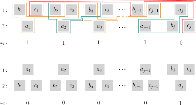
Figure 3: Improving $\sigma$ by making $\omega_{j}=1$ and $\omega_{i}=0$ for any $j\in\{3,...,n\}$ and all $i\in\{1,...,j-1\}$.

Lemma 3.4.

Suppose we have $\omega_{1}=0$ and $\ell\in M_{1}$. Then, $\sigma$ can be improved by making $\omega_{1}=1$.

Proof.

For $\omega_{1}=0$, we have $a_{1}\in M_{1}$ and $b_{1},c_{1}\in M_{2}$. Since $\Delta$ has a very large value, we just need to show that $p_{a_{1}}$ is greater than $p_{b_{1}}+p_{c_{1}}$. We have $p_{a_{1}}-p_{b_{1}}-p_{c_{1}}=2^{n}$, which is greater than 0. Therefore, by swapping $a_{1}$ with $b_{1}$ and $c_{1}$, and making $\omega_{1}=1$, we improve the schedule. ∎

Next, we show that we are able to improve the schedule by moving $a_{1},b_{2}$ and $c_{2}$ to $M_{1}$, and $b_{1},c_{1}$ and $a_{2}$ to $M_{2}$.

Lemma 3.5.

Let $\sigma$ be scheduled with $\omega_{1}=1$, $\omega_{2}=0$ and $\ell\in M_{1}$. Then, $\sigma$ can be improved by making $\omega_{1}=0$ and $\omega_{2}=1$.

Proof.

For $\omega_{1}=1$ and $\omega_{2}=0$, we have $a_{2},b_{1},c_{1}\in M_{1}$ and $a_{1},b_{2},c_{2}\in M_{2}$. We have $p_{a_{2}}-p_{a_{1}}-p_{b_{2}}=1>0$ and $p_{b_{1}}+p_{c_{1}}-p_{c_{2}}=2^{n}-1>0$. Therefore, first we swap $a_{2}$ with $a_{1}$ and $b_{2}$, and then, we swap $b_{1}$ and $c_{1}$ with $c_{2}$. Note that $\Delta$ has a large value, which means that these two swaps improve the schedule. After performing these swaps, we get $\omega_{1}=0$ and $\omega_{2}=1$. ∎

Finally, we have the following lemma.

Lemma 3.6.

Let $j\in\{3,...,n\}$ with $\omega_{j}=0$. For all $i\in\{1,...,j-1\}$, we have $\omega_{i}=1$. Also, we have $\ell\in M_{1}$. Then, $\sigma$ can be improved by making $\omega_{j}=1$ and $\omega_{i}=0$ for all $i\in\{1,...,j-1\}$.

Proof.

We have $b_{i},c_{i},a_{j}\in M_{1}$ and $a_{i},b_{j},c_{j}\in M_{2}$ when $\omega_{j}=0$ and $\omega_{i}=1$ for all $i\in\{1,...,j-1\}$ (see Fig. 3). We have $p_{a_{j}}-p_{a_{j-1}}-p_{b_{j}}=2^{j-2}>0$. Therefore, we are able to swap $a_{j}$ with $a_{j-1}$ and $b_{j}$. Also, we have $p_{b_{k}}+p_{c_{k+1}}-p_{a_{k}}=2^{k-1}>0$ for all $k\in\{1,...,j-2\}$. Therefore, we are able to improve $\sigma$ by swapping $b_{k}$ and $c_{k+1}$ with $a_{k}$ for all $k\in\{1,...,j-2\}$. Moreover, we have $p_{b_{j-1}}+p_{c_{1}}-p_{c_{j}}=2^{n}+1-2^{j-1}>0$. So, we improve the schedule by swapping $b_{j-1}$ and $c_{1}$ with $c_{j}$ (see Fig. 3). After all these swaps, we get $\omega_{j}=1$ and $\omega_{i}=0$ for all $i\in\{1,...,j-1\}$. ∎

According to Lemma 3.4, Lemma 3.5, and Lemma 3.6, we have all the combinations of zeros and ones for the tuple $(\omega_{1}(\sigma),\dotsc,\omega_{n}(\sigma))$. Therefore, we have the following theorem.

Theorem 3.7.

The number of improving 3-swaps until a 3-swap optimal solution is reached can be $2^{\Omega(n)}$.

4 Computational Results

The focus of this paper was on approaching the problem $P2||C_{max}$ with local search by considering the $k$-swap neighborhood. In this part, we conduct computational experiments on various families of instances, where certain scenarios involve more than two machines. The reason for considering more than two machines in some cases is to get some insight into the total number of iterations in finding a local optimum. First, we delve into the empirical behavior of the running time of the randomized algorithm proposed in this paper by comparing this algorithm with the naive approach in searching the $k$-swap neighborhood. Subsequently, we examine the total number of iterations needed to find a $k$-swap optimal solution. In this regard, we have considered 9 classes of instances $C_{1},C_{2},\dotsc,C_{9}$, each of which consists of 50 instances. The instances of each class are generated with respect to two parameters $n$ and $m$, which are the number of jobs and machines in that class, respectively (see Table 1 for an overview). Moreover, for the processing time of each job, we have chosen an integer uniformly at random from the range $[1,10^{9}]$.

Table 1: An overview on the different classes of instances.

	$C_{1}$	$C_{2}$	$C_{3}$	$C_{4}$	$C_{5}$	$C_{6}$	$C_{7}$	$C_{8}$	$C_{9}$
$n$	50	100	200	50	100	200	50	100	200
$m$	2	2	2	5	5	5	10	10	10
max $k$	9	6	5	9	6	5	9	6	5

Table 2: Average values of the running time (in milliseconds) of the randomized and naive operators for different values of $k$ in different classes of instances.

	$k$	$C_{1}$	$C_{2}$	$C_{3}$	$C_{4}$	$C_{5}$	$C_{6}$	$C_{7}$	$C_{8}$	$C_{9}$
Randomized	1	$<0.1$	0.3	0.3	1.6	0.6	3.1	1.2	0.3	2.2
Naive	1	$<0.1$	$<0.1$	$<0.1$	$<0.1$	$<0.1$	$<0.1$	$<0.1$	$<0.1$	0.3
Randomized	2	0.2	0.8	0.3	0.3	1.2	0.9	0.3	0.7	0.5
Naive	2	$<0.1$	0.2	2.6	0.1	0.8	0.6	0.5	0.3	0.4
Randomized	3	2.2	3.4	10.6	0.4	1.1	2.8	0.4	0.6	1.4
Naive	3	0.6	2.9	15.5	0.2	0.9	4.0	0.1	0.2	1.2
Randomized	4	1.6	6.5	24.4	0.6	1.7	4.9	0.5	0.8	2.3
Naive	4	3.8	26.3	288.9	0.5	3.8	37.2	0.1	0.8	6.4
Randomized	5	7.2	38.2	232.3	1.0	4.2	23.8	0.5	1.4	6.7
Naive	5	13.0	264.7	15367.4	1.1	14.7	426.2	0.3	1.8	32.5
Randomized	6	13.3	78.6	-	1.4	7.4	-	0.6	1.9	-
Naive	6	53.8	2691.2	-	2.2	59.0	-	0.2	3.2	-
Randomized	7	35.2	-	-	2.0	-	-	0.7	-	-
Naive	7	220.6	-	-	3.3	-	-	0.3	-	-
Randomized	8	61.6	-	-	2.6	-	-	0.7	-	-
Naive	8	793.1	-	-	4.7	-	-	0.5	-	-
Randomized	9	150.3	-	-	3.5	-	-	0.8	-	-
Naive	9	2250.4	-	-	5.5	-	-	0.4	-	-

Table 3: Average number of iterations of the randomized and naive operators for different values of $k$ in different classes of instances.

	$k$	$C_{1}$	$C_{2}$	$C_{3}$	$C_{4}$	$C_{5}$	$C_{6}$	$C_{7}$	$C_{8}$	$C_{9}$
Randomized	1	0.0	0.3	0.3	1.6	0.6	3.1	1.2	0.3	2.2
Naive	1	0.0	0.0	0.0	0.0	0.0	0.0	0.0	0.0	0.3
Randomized	2	0.2	0.8	0.3	0.3	1.2	0.9	0.3	0.7	0.5
Naive	2	0.0	0.2	2.6	0.1	0.8	0.6	0.5	0.3	0.4
Randomized	3	2.2	3.4	10.6	0.4	1.1	2.8	0.4	0.6	1.4
Naive	3	0.6	2.9	15.5	0.2	0.9	4.0	0.1	0.2	1.2
Randomized	4	1.6	6.5	24.4	0.6	1.7	4.9	0.5	0.8	2.3
Naive	4	3.8	26.3	288.9	0.5	3.8	37.2	0.1	0.8	6.4
Randomized	5	7.2	38.2	232.3	1.0	4.2	23.8	0.5	1.4	6.7
Naive	5	13.0	264.7	15367.4	1.1	14.7	426.2	0.3	1.8	32.5
Randomized	6	13.3	78.6	-	1.4	7.4	-	0.6	1.9	-
Naive	6	53.8	2691.2	-	2.2	59.0	-	0.2	3.2	-
Randomized	7	35.2	-	-	2.0	-	-	0.7	-	-
Naive	7	220.6	-	-	3.3	-	-	0.3	-	-
Randomized	8	61.6	-	-	2.6	-	-	0.7	-	-
Naive	8	793.1	-	-	4.7	-	-	0.5	-	-
Randomized	9	150.3	-	-	3.5	-	-	0.8	-	-
Naive	9	2250.4	-	-	5.5	-	-	0.4	-	-

We have implemented both the randomized and naive $k$-swap operators in Python 3.10.6 programming language, and we have executed them on a computer with a 2.40GHz Intel Core i5 CPU and 8,00 GB of RAM under the Windows 10 operating system. Our implementation and our instances are publicly available on GitHub [28].

To do the experiments, we have executed the randomized and naive operators for different values of $k$ on all the 450 instances that we have (see Table 1 for the maximum value of $k$ in each class). To compute the average running time of the randomized and naive operators for an instance $i$ of a class $C_{j}$ and a value $k$, we start from an initial solution computed by the longest processing time first ($LPT$) algorithm [16], and then, we divide the total running time by the number of iterations in finding a $k$-swap optimal solution with respect to these two operators. Note that according to Lemma 2.1, when we are not able to find an improving solution by the randomized $k$-swap algorithm, we need to run it at most $\dfrac{2^{k}}{\binom{k}{\lceil\frac{k}{2}\rceil}}$ times to amplify the probability of success of the algorithm. Finally, to calculate the average running time of the randomized and naive operators for a class $C_{j}$ and a value $k$, we compute the average value of the average running times of the randomized and naive operators over all the instances in the class $C_{j}$ for the value $k$, respectively. For our detailed results, see Table 2 and Table 3.

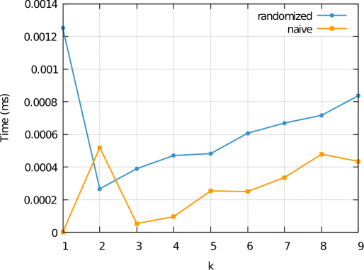
Figure 4: Average running time (in milliseconds) of the randomized and naive operators for different values of $k$ in class $C_{7}$.

We can observe that in most of the classes by increasing the value of $k$, the randomized operator is capable of finding an improving neighbor faster than the naive one (see Table 2). However, in some cases such as in class $C_{7}$, the running time of the naive operator is less than the randomized operator even for larger values of $k$ (see Fig. 4). More precisely, in classes where we have relatively more jobs on each machine, the randomized operator is able to find an improving neighbor faster than the naive one. Also, when we increase the value of $k$, the gap between the running times of these two operators increases (see Fig. 5). As a matter of fact, for finding an improving neighbor in the $k$-swap neighborhood, the naive operator only searches the neighborhood, however, the randomized operator performs some preprocessing first and after that searches a smaller neighborhood. Therefore, when we have relatively fewer jobs on each machines, it is better to use the naive operator to find an improving neighbor, and when we have more jobs, by using the randomized operator, we are able to find a solution faster.

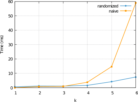
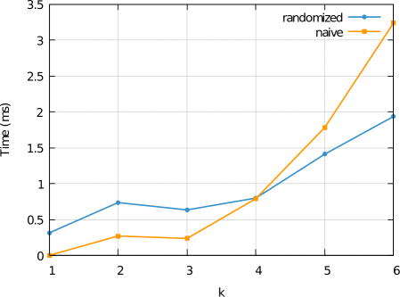
Figure 5: Average running time (in milliseconds) of the randomized and naive operators for different values of $k$ in classes $C_{5}$ (left diagram) and $C_{8}$ (right diagram).

In Theorem 3.3, we provided a polynomial upper bound for the number of iterations in finding a 2-swap optimal solution when we have two machines in our schedule. According to our computational results, we do not observe any significant increase in the number of iterations when the number of machines is 5 and 10 (see Table 3). This computational result raises the question if it is possible to establish a polynomial upper bound on the number of iterations when dealing with schedules involving more than two machines. Moreover, in Theorem 3.7, we established an exponential lower bound for the case of swapping 3 jobs in each iteration. The computational experiments in Table 3 lead us to question whether the establishment of this lower bound reflects an exceptionally pessimistic scenario. In other words, the occurrence of such a scenario might be rare in practice.

5 Concluding Remarks

The main focus of this paper was to approach the problem $P2||C_{\max}$ by a local search neighborhood, called $k$-swap, both theoretically and practically. To find an improving solution in this neighborhood, we proposed a randomized algorithm that is capable of finding such a solution faster than the naive approach in searching the neighborhood. We proposed this algorithm for the case of having only two machines in our schedule; however, in the computational results, we have run this algorithm for some scenarios in which more than two machines are involved. As a matter of fact, this algorithm is extendable to the case of having more than two machines by repeating all the steps for all the pairs of critical and non-critical machines, which adds a factor of $O(m^{2})$ to the running time of this algorithm.

Additionally, we established an upper bound of $O(n^{4})$ on the number of local search steps required to converge to a local optimum for $k=2$ when we have only two machines, and according to the computational results, it is interesting to see if it is possible to provide a polynomial upper bound for the case of having more than two machines. Furthermore, we provided an exponential lower bound for the case of swapping 3 jobs in each step. The computational results raise the question of whether the lower bound reflects a pessimistic scenario. In practice, the occurrence of such a scenario might be rare.

References

- [1] E.H. Aarts and J.K. Lenstra. Local search in combinatorial optimization. Princeton University Press, 2003.
- [2] A. Abboud and K. Lewi. Exact weight subgraphs and the k-sum conjecture. In International Colloquium on Automata, Languages, and Programming (ICALP), pages 1–12. Springer, 2013.
- [3] R.K. Ahuja, J.B. Orlin, and D. Sharma. Multi-exchange neighborhood structures for the capacitated minimum spanning tree problem. Mathematical Programming, 91(1):71–97, 2001.
- [4] N. Alon, R. Yuster, and U. Zwick. Color-coding. Journal of the ACM, 42(4):844–856, 1995.
- [5] M.D. Berg, K. Buchin, B.M Jansen, and G. Woeginger. Fine-grained complexity analysis of two classic tsp variants. ACM Transactions on Algorithms, 17(1):1–29, 2020.
- [6] S. Berndt, M.A. Deppert, K. Jansen, and L. Rohwedder. Load balancing: The long road from theory to practice. In 2022 Proceedings of the Symposium on Algorithm Engineering and Experiments (ALENEX), pages 104–116. SIAM, 2022.
- [7] P. Brucker, J. Hurink, and F. Werner. Improving local search heuristics for some scheduling problems—i. Discrete Applied Mathematics, 65(1-3):97–122, 1996.
- [8] P. Brucker, J. Hurink, and F. Werner. Improving local search heuristics for some scheduling problems. part ii. Discrete Applied Mathematics, 72(1-2):47–69, 1997.
- [9] T. Brueggemann, J.L. Hurink, T. Vredeveld, and G.J. Woeginger. Exponential size neighborhoods for makespan minimization scheduling. Naval Research Logistics, 58(8):795–803, 2011.
- [10] G.A. Croes. A method for solving traveling-salesman problems. Operations research, 6(6):791–812, 1958.
- [11] D. Dumrauf, B. Monien, and K. Tiemann. Multiprocessor scheduling is pls-complete. In 2009 42nd Hawaii International Conference on System Sciences, pages 1–10. IEEE, 2009.
- [12] G. Finn and E. Horowitz. A linear time approximation algorithm for multiprocessor scheduling. BIT Numerical Mathematics, 19(3):312–320, 1979.
- [13] M.M. Flood. The traveling-salesman problem. Operations research, 4(1):61–75, 1956.
- [14] A. Frangioni, E. Necciari, and M.G. Scutella. A multi-exchange neighborhood for minimum makespan parallel machine scheduling problems. Journal of Combinatorial Optimization, 8(2):195–220, 2004.
- [15] R.L. Graham. Bounds for certain multiprocessing anomalies. Bell system technical journal, 45(9):1563–1581, 1966.
- [16] R.L. Graham. Bounds on multiprocessing timing anomalies. SIAM journal on Applied Mathematics, 17(2):416–429, 1969.
- [17] R.L. Graham, E.L. Lawler, J.K. Lenstra, and A.R. Kan. Optimization and approximation in deterministic sequencing and scheduling: a survey. In Annals of discrete mathematics, volume 5, pages 287–326. Elsevier, 1979.
- [18] D.S. Hochbaum and D.B. Shmoys. Using dual approximation algorithms for scheduling problems theoretical and practical results. Journal of the ACM, 34(1):144–162, 1987.
- [19] E. Horowitz and S. Sahni. Computing partitions with applications to the knapsack problem. Journal of the ACM, 21(2):277–292, 1974.
- [20] C.A. Hurkens and T. Vredeveld. Local search for multiprocessor scheduling: how many moves does it take to a local optimum? Operations Research Letters, 31(2):137–141, 2003.
- [21] D.S. Johnson and M.R. Garey. Computers and intractability: A guide to the theory of NP-completeness. WH Freeman, 1979.
- [22] J.K. Lenstra, D.B. Shmoys, and É. Tardos. Approximation algorithms for scheduling unrelated parallel machines. Mathematical programming, 46:259–271, 1990.
- [23] Y.L. Luke. Special Functions and Their Approximations: v. 2. Academic press, 1969.
- [24] D. Marx. Parameterized complexity and approximation algorithms. The Computer Journal, 51(1):60–78, 2008.
- [25] W. Michiels, E.H. Aarts, and J. Korst. Theoretical aspects of local search, volume 13. Springer, 2007.
- [26] R. Motwani and P. Raghavan. Randomized algorithms. Cambridge university press, 1995.
- [27] M. Naor, L.J. Schulman, and A. Srinivasan. Splitters and near-optimal derandomization. In Proceedings of IEEE 36th Annual Foundations of Computer Science (FOCS), pages 182–191. IEEE, 1995.
- [28] L. Rohwedder, A. Safari, and T. Vredeveld. Implementation of the randomized and naive -swap algorithms. https://github.com/a-safari/k-swap, 2024.
- [29] S.K. Sahni. Algorithms for scheduling independent tasks. Journal of the ACM, 23(1):116–127, 1976.
- [30] P. Schuurman and T. Vredeveld. Performance guarantees of local search for multiprocessor scheduling. INFORMS Journal on Computing, 19(1):52–63, 2007.
- [31] G.J. Woeginger. When does a dynamic programming formulation guarantee the existence of a fully polynomial time approximation scheme (fptas)? INFORMS Journal on Computing, 12(1):57–74, 2000.