adedieu@deepmind.com
Learning Cognitive Maps from Transformer Representations for Efficient Planning in Partially Observed Environments
Abstract
Despite their stellar performance on a wide range of tasks, including in-context tasks only revealed during inference, vanilla transformers and variants trained for next-token predictions (a) do not learn an explicit world model of their environment which can be flexibly queried and (b) cannot be used for planning or navigation. In this paper, we consider partially observed environments (POEs), where an agent receives perceptually aliased observations as it navigates, which makes path planning hard. We introduce a transformer with (multiple) discrete bottleneck(s), TDB, whose latent codes learn a compressed representation of the history of observations and actions. After training a TDB to predict the future observation(s) given the history, we extract interpretable cognitive maps of the environment from its active bottleneck(s) indices. These maps are then paired with an external solver to solve (constrained) path planning problems. First, we show that a TDB trained on POEs (a) retains the near-perfect predictive performance of a vanilla transformer or an LSTM while (b) solving shortest path problems exponentially faster. Second, a TDB extracts interpretable representations from text datasets, while reaching higher in-context accuracy than vanilla sequence models. Finally, in new POEs, a TDB (a) reaches near-perfect in-context accuracy, (b) learns accurate in-context cognitive maps (c) solves in-context path planning problems.
1 Introduction
Large vanilla transformers (Vaswani et al., 2017) trained for next-token prediction have been successfully applied to a wide range of applications such as natural language processing (Radford et al., 2018; Chowdhery et al., 2022), text-conditioned image generation (Ramesh et al., 2021), reinforcement learning (Chen et al., 2021a), code writing (Chen et al., 2021b). These large language models (LLMs) also exhibit emergent abilities (Wei et al., 2022), among which their capacity to in-context learn (ICL), i.e., to adapt to a new task at inference time given a few examples (Brown et al., 2020). However, these models suffer from shortcomings that prevent them from being used for planning and navigation (Valmeekam et al., 2022; Mialon et al., 2023). In particular, they do not learn an interpretable world model (Momennejad et al., 2023) which can be flexibly queried.
Herein, we consider a suite of partially observed environments (POEs) Chrisman (1992) where the agent receives perceptually aliased observations as it navigates; and cannot deterministically recover its spatial positions from its observations. Path planning in these POEs is hard: the planner has to disambiguate aliasing to locate itself, which requires modeling its history of observations and actions.
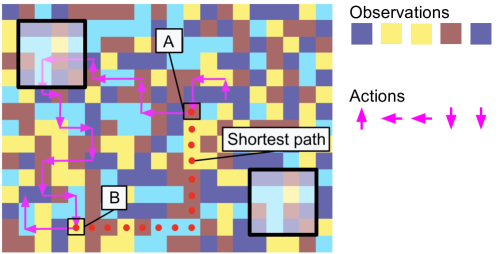
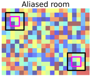
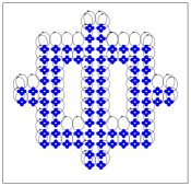
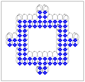
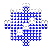
Example of a path planning problem in a POE that a vanilla transformer cannot solve: We consider the partially observed room in Fig.1, which only contains four unique observations. The room also has global aliasing: the patch with a black border appears twice. An agent executes a series of discrete actions, each action leading to a discrete observation. The agent does not have access to any reward or to the room layout. At test time, it wants to find a shortest path (in red) between two room positions (A and B) it has been to. A transformer trained to predict the next observation given past observations and actions can only perform forward rollouts, which, due to aliasing, (a) scale exponentially in the distance between A and B (b) prevents it from even knowing when it reaches the target B.
In this paper, we propose the transformer with discrete bottleneck(s), TDB), which adds a single, or multiple, discrete bottleneck(s) (Van Den Oord et al., 2017) on top of a transformer to compress the transformer outputs into a finite number of latent codes. We train TDB with an augmented objective, then extract a cognitive map from its active bottleneck(s) indices. First, we show that, on aliased rooms, aliased cubes with non-Euclidean dynamics and visually rich D environments (Beattie et al., 2016), these maps (a) disambiguate aliasing (b) nearly recover the ground truth dynamics and (c) can be paired with external solvers to solve path planning problems—like the one in Fig.1. Hence, TDB (a) retains the nearly perfect predictive abilities of vanilla transformers and LSTMs, (b) solves (constrained) path planning problems exponentially faster. Second, a TDB extracts an interpretable latent graph from a text dataset (Xie et al., 2021) while achieving higher test accuracies than vanilla sequence models. Finally, when exploring a new POE at test time, TDB can (a) in-context predict the next observation given history (b) solve in-context path planning problems (c) learn accurate in-context cognitive maps.
2 Related work
Planning with LLMs: Despite their success on simple benchmarks including maths (Cobbe et al., 2021) and logics (Srivastava et al., 2022), growing evidence suggests that LLMs performance collapse on benchmarks that require stronger planning skills (Valmeekam et al., 2022). While Pallagani et al. (2022) finetune LLMs for planning, Guan et al. (2023) extract an approximate world model with an LLM, then further refine it with an external planner.
Interpretable circuits: Some works try to reverse-engineer LLMs to extract interpretable circuits, i.e., internal structures that drive certain model behaviors (Elhage et al., 2021; Olsson et al., 2022; Nanda et al., 2023). While circuit analysis can be performed at scale (Lieberum et al., 2023), it is labor intensive (Conmy et al., 2023), and does not extract explicit structures to solve planning or navigation tasks.
Decision transformers: Decision transformers (Chen et al., 2021a) abstract reinforcement learning (RL) as sequence modeling: they can play Atari games and stack blocks with a robot arm (Reed et al., 2022). However, they only have been applied to shortest path problems on small graphs with nodes. Decision transformers have also access to a reward, which reveals information about the environment. They would struggle to solve the shortest path in Fig.1, where aliasing is high and no external reward is provided.
Learning world models with a transformer: Lamb et al. (2022) train a transformer with a multi-step objective on sequences of observations and actions, and successfully learned a minimal world representation that either the agent can control or that affects its dynamics. However, the authors (a) consider fully visible settings and (b) learn representations by discarding the agent’s history: their approach would not solve the shortest path in aliased settings as in Fig.1. In another approach, Guo et al. (2022) learn future latent representations from current latent representations but do not explicitly extract interpretable world models that can be used for planning. In a different line of work, Li et al. (2022) show that transformers learn internal world models, that can be used to control some model’s behavior. In contrast, here, we are interested in extracting a world model from a transformer that can be used to solve path planning problems exponentially faster than vanilla models.
Clone-structured causal graphs (CSCGs): CSCG (George et al., 2021) is an interpretable probabilistic model that learns cognitive maps in aliased POEs and solves path planning tasks. However, CSCGs learn a block-sparse transition matrix over a large latent space via the expectation-maximization (EM) algorithm (Dempster et al., 1977). This large transition matrix occupies a large amount of memory and limits CSCGs’ scalability—see Appendix B.1 for a detailed discussion. CSCGs would also struggle to solve the ICL experiments in Sec.4.5 without an external algorithm—see Swaminathan et al. (2023). In contrast, the transformer variant we introduce in this paper builds this same transition matrix sparsely, via local counts. Appendix B.2 discusses a CSCG-inspired variant of our proposed model.
3 A path planning-compatible transformer
3.1 Problem statement
Problem: We consider an agent executing a series of discrete actions with , e.g. walking in a room. As a result of each action, the agent receives a perceptually aliased observation Chrisman (1992), resulting in the stream . The agent does not have access to any reward at any time. Our goal is to (a) predict the next observation given the history of past observations and actions and (b) build a world model that disambiguates aliased observations and that can be called by an external planner to solve path planning tasks.
Trajectory representation: We represent a trajectory by alternating observations and actions. This representation allows us to consider the autoregressive objective of predicting the next observation given the history of past observations and actions:
| (1) |
3.2 Predicting the next observation with a transformer
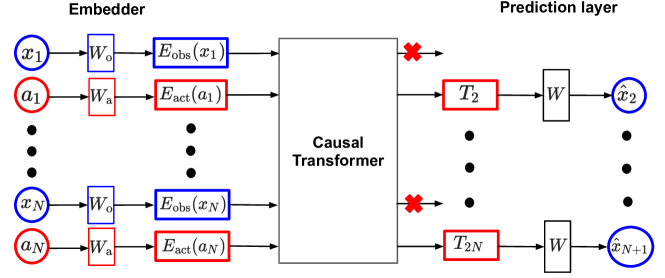
We propose to train a vanilla transformer (Vaswani et al., 2017) to minimize Equation (1). To do so, we first map each categorical observation (resp. action ) of to a linear embedding (resp. ). Second, we feed the sequence of input embeddings to a transformer with causal mask (Radford et al., 2018), resulting in the output sequence . We only retain the outputs with even indices : is derived after applying the successive self-attention layers to the intermediate representations of . Finally, a linear mapping applied to returns the predicted logits for the next observation . We display this transformer architecture in Fig.6, Appendix A.
As we show in Sec.4, this transformer almost perfectly predicts the next observation on a suite of perceptually aliased POEs. However, it can only solve the path planning problem in Fig.1 with forward rollouts, which have an exponential cost in the distance between the room positions A and B.
3.3 A transformer with a discrete bottleneck
To address these inherent limitations, we add a discrete bottleneck on top of a vanilla transformer, which compresses all the information needed to minimize Equation (1).
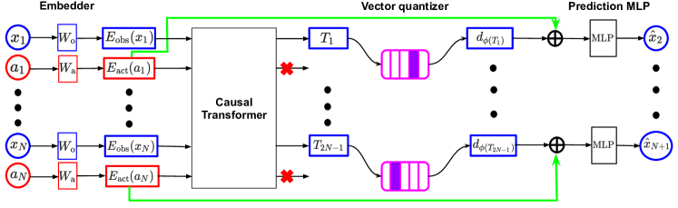
After applying the causal transformer from Sec.3.2 to the sequence of observations and actions embeddings, we now only extract the encodings with odd indices, which results in the stream : is derived from , but is not aware of the action . We then apply vector quantization (Van Den Oord et al., 2017) and map each vector to the closest entry in a dictionary of latent codes , where . That is, we introduce the operator
| (2) |
The quantized output of is . Because has not been exposed to , we derive the next observations logits via , where is a two layers MLP and represents the concatenation operator. We refer to our proposed transformer with a discrete bottleneck as TDB, and visualize it in Figure 2.
3.4 Augmenting the objective value
The discrete bottleneck in Sec.3.3 introduces the additional objective term with
| (3) |
where , and the stop-gradient operator (Van Den Oord et al., 2017). However, we show in Fig.7, Appendix G that a TDB trained with the simple objective fails at disambiguating observations with identical neighbors. To allow the TDB to learn richer representations of the observations, we propose to augment the transformer objective via two solutions.
Solution 1: Predicting the next observations. At each timestep , instead of only predicting the next observation—which corresponds to —we predict the next observations and replace the loss in Equation (1) with
| (4) |
The model does not have access to any observation after : it only sees the actions . The logits of the observation are predicted via , where is a two-layers MLP. In Sec.4, we set .
Solution 2: Predicting the next encoding. Our second solution is to predict future latent representations Guo et al. (2022). We refer to the TDB described so far as a student network, with weights , and introduce a teacher network (Grill et al., 2020), with the same architecture and whose weights are an exponential moving average of . At each gradient update, we set , where is the decay rate, which we fix to .
The student network predicts both (a) the next observation and (b) the next teacher network’s quantized encoding. This introduces the objective term with
where is a two-layer MLP with same hidden layer as .
3.5 Extension to multiple discrete bottlenecks
TDB supports discrete bottlenecks. Each bottleneck induces its own (a) dictionary of latent codes , (b) function which acts as in Equation (2) and (c) objective . The transformer output passes through the discrete bottlenecks in parallel: the th bottleneck returns the latent code . We get back to the previous case by defining (a) and (b) . As we show in Sec.4, multiple discrete bottlenecks make training faster and sometimes better. However, Appendix F introduces a disentanglement metric which shows that they are highly redundant and do not learn disentangled representations.
3.6 Learning a cognitive map from bottleneck indices
When we use a single bottleneck, TDB maps each observation to the latent code index . We define a count tensor which counts the empirical latent transitions: . We then threshold to build an action-augmented empirical transition graph . That is, has an edge between the vertices and with the action iff. , where and is a threshold. This edge indicates that the action leads from the latent node to the latent node a large number of times.
In practice (a) we use multiple discrete bottlenecks (see Sec.3.5) and cluster the bottleneck indices using the Hamming distance with a threshold and (b) we map each discarded node of to a retained node in so that we can solve all the path planning problems in Sec.4. We detail (a) and (b) in Appendix C. As a result, each node in is paired with a collection of tuples of bottleneck indices.
is a cognitive map of the agent’s environment which (a) is interpretable, (b) is action-conditioned, hence, models the agent’s dynamics, and (c) can be paired with an external planner to solve path planning problems—see Sec.4.
3.7 Why does TDB learn an accurate map?
The TDB latent index associated with an observation given its history corresponds to a node in the latent graph in Sec.3.6. For to correctly model the environment’s dynamics, when this node is active, the agent must always be at the same ground truth spatial position.
does not know the next action ; and compresses all the information needed to minimize the loss at the th step. When TDB predicts the next observation, must then encode the next observation that each next possible action leads to. As we show in Appendix G, may not disambiguate distinct spatial positions with identical neighbors. When TDB predicts the next observations (Solution 1, Sec.3.4), must now encode all the observations that each sequence of actions leads to. For a large , the latent index is encouraged to only be active at a unique spatial location. An alternative approach is to augment so that it compresses all its neighbors’ encoding (Solution 2).
4 Computational results
We assess the performance of our proposed TDB on four experiments: (a) synthetic D aliased rooms and aliased cubes, (b) simulated D environments, (c) text datasets and (d) mixtures of D aliased rooms. Each experiment is run on a grid of Tensor Processing Unit v2.
4.1 Methods compared
Each experiment compares the following methods:
The causal transformer described in Sec.3.2, trained with the autoregressive objective in Equation (1). The architecture considered has layers, attention heads, a context length of , an embedding dimension of , and an MLP hidden layer dimension of . We use relative positional embedding (Dai et al., 2019) and Gaussian error linear units activation functions (Hendrycks and Gimpel, 2016).
Several TDBs, using the same causal transformer. We refer to each model as TDB where (a) is the number of prediction steps (Solution 1, Sec.3.4), (b) is the number of discrete bottlenecks (see Sec.3.5)—each one contains latent codes. We note TDB when we predict the next encoding (Solution 2, Sec.3.4). After training, we build a cognitive map as in Sec.3.6 using .
A vanilla LSTM (Hochreiter and Schmidhuber, 1997) with hidden dimension of 256.
4.2 Random walks in 2D aliased rooms
Problem: We consider a D aliased ground truth (GT) room of size , containing unique observations, and a patch repeated twice—similar to Fig.1. An agent walking selects, at each timestep, a discrete action and collects the categorical observation . The actions have unknown semantics: the agent does not know that corresponds to moving up. No assumptions about Euclidean geometry are made either. The training and test set contains random walks of observations and actions of length each.
Training: We train each method in Sec.4.1 with Adam (Kingma and Ba, 2014) for k training iterations, using a learning rate of and a batch size of . For regularization, we use a dropout of .
Solving path planning problems at test time: For a test sequence of length , let be the GT unknown D spatial position of the observation . At test time, given a context , the path planning task is to derive a shortest path, i.e. a sequence of actions, which leads from to in the GT room. We emphasize that (a) the model only observes and does not know (b) the path is a solution, referred to as fallback path. Fig.1 shows this problem for .
For a vanilla sequence model, we autoregressively sample random rollouts of length each and collect all the candidates, i.e., the observations equal to . Because of aliasing, the model cannot know whether a candidate is at the target position . We use the tail of the last observations and actions and only return the candidates estimated to be at . For a TDB, after learning the cognitive map , we map and to the bottleneck indices and , then to two nodes of using the Hamming distance. We then call the external solver networkx.shortest_path (Hagberg et al., 2008) to find the shortest path between these two nodes. See Appendix D for details about both procedures.
Metrics:
We evaluate each method for four metrics.
A prediction metric, TestAccu: next observation accuracy on the test random walks.
Two path planning metrics: we consider shortest paths problems and report (a) ImpFallback, the percentage of problems for which a model finds a valid path which improves over the fallback path—a path (i.e. a sequence of actions) is valid if it correctly leads from to in the GT room—and (b) RatioSP, when a better valid path is found, the ratio between its length and an optimal path length—we derive an optimal path using the GT room.
Normalized graph edit distance, defined for two graphs as
where GED is the graph edit distance (Sanfeliu and Fu, 1983) and is the empty graph. NormGED is lower than and is equal to iff. and are isomorphic. We use a timeout of minutes and empirical positions to accelerate the GED computation—see Appendix H.
| Method | TestAccu () | ImpFallback () | RatioSP | NormGED |
|---|---|---|---|---|
| Vanilla transformer | — | |||
| Vanilla LSTM | — | |||
| TDB | ||||
| TDB | ||||
| TDB | ||||
| TDB |
Results: Table 1 averages the metrics over experiments: each run considers a different GT room. First, we observe that both vanilla LSTM and transformer almost perfectly predict the next observation given the history. However, both sequence models struggle to solve path planning problems with forward rollouts: they only improve over the fallback path of the same. When they do so, they find shorter paths times longer than an optimal path1.
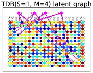
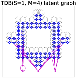
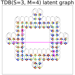
Second, all the TDBs retain the predictive performance of vanilla models. However, TDB fails at path planning: it only finds better valid paths of the time as it only solves the simplest problems. Indeed, the learned cognitive maps merge the observations with identical neighbors, which introduces unrealistic shortcuts in the latent graphs—see Fig.7, Appendix G. In contrast, TDB with either (a) multi-step or (b) next encoding objective learns cognitive maps that recover the GT dynamics and reach low NormGED—see Fig.3[center left]. They are able to almost consistently find an optimal shortest path. As a result, ImpFallback is above while RatioSP is .
Multiple discrete bottlenecks accelerate training: Table 2, Appendix E, reports the average number of training steps to reach a train accuracy: for , this number goes from for down to for . In addition, multiple discrete bottlenecks seem more robust to the environment. Table 6, Appendix I.2, shows that, when the room contains unique observations, all the TDBs with outperform their counterparts.
Lack of disentanglement in the latent space: We test whether multiple discrete bottlenecks learn a disentangled representation by training a logistic regression to predict each bottleneck index given the other indices—see Appendix F for details. If the bottlenecks were independent, test disentanglement accuracy would be . However, it is , which shows the strong redundancy in the representations learned by each bottleneck.
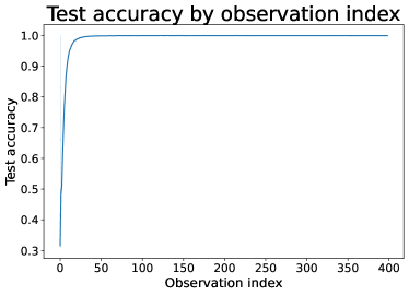
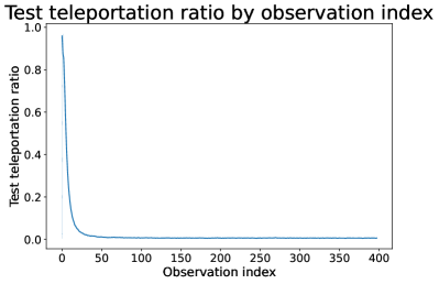
The agent can locate itself after a short context: Appendix I.3 first shows that, on test random walks, accuracy is initially low then quickly increases: it is above after the th observation—see Fig.9. Second, latent codes have a bimodal distribution: many codes with low empirical frequencies model the agent’s early uncertainty and are replaced by high-frequency latent codes which later express the agent’s confidence—see Fig.10. Finally, the agent can “teleportate” in the room but such behavior appears less than of the time after the th observation—see Fig.11.
TDB can solve constrained path planning problems: TDB can inject constraints on demand into the external solver. To illustrate this, we consider a path planning problem variant: the new task is to find the shortest path from to which avoids, when possible, a randomly picked color. TDB is still able to almost consistently solve the problem: ImpFallback is still while RatioSP is still . The average length of the shortest paths is now , as opposed to when all the colors are allowed.
TDB handles noise during training: When replacing of the training observations of a TDB by random ones, training accuracy drops to , while TestAccu, ImpFallback and RatioSP are still and , showing that training noise does not affect the test prediction and planning performance.
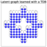
TDB learn maps for non-Euclidean dynamics: TDB can be applied to aliased environments with non-Euclidean dynamics. We generate data from a D aliased cube with edge size and unique observations—see Fig.3[bottom left]. Table 5, Appendix I.1 shows that the prediction and planning performance of a TDB are near perfect. Fig.3[bottom - center left] visualizes the learned graph with the Kamada-Kawai algorithm (Kamada et al., 1989),
|
|


|
 |
 |
4.3 Egocentric views in 3D simulated environments
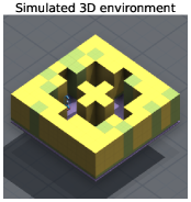
Problem: We consider a suite of visually rich D simulated environments (Beattie et al., 2016) with a similar setting as Guntupalli et al. (2023)—see Fig.3[center, center right]. At each step, the agent can take any of three discrete egocentric actions—move m forward, rotate left, rotate right—and it sees a new view, which is a RGB image. The agent’s egocentric views are clustered with a -means quantizer—with — and the clusters indices are used as categorical observations. The training and test set sizes are identical to Sec.4.2.
Training: We train the same models as in Sec.4.2, with the same parameters, on synthetic D rooms.
Results: The full results are reported in Table 7, Appendix J. Despite their excellent predictive performance, vanilla sequence models only find a path better than fallback for of the problems: these “better” paths are times longer than optimal paths111The transformer and LSTM performance are almost identical because the same random walks are used for both models.. Compared with Sec.4.2, training TDBs with a single bottleneck do not converge. Consequently, these models reach a low test accuracy and cannot solve the path planning problems. In contrast, for TDBs with discrete bottlenecks, averaged train accuracies are at least after only training steps (see Table 3, Appendix E). These models reach nearly perfect (a) test accuracy and (b) path planning performance. Their latent maps accurately model the POE’s dynamics—see Fig.3[right] and Fig.12, Appendix J. However, the multiple bottlenecks learn a highly redundant representation: the test disentanglement accuracy (see Appendix F) of a TDB is .
4.4 Extension to text via the GINC dataset
Problem: Herein, we extend TDB to text datasets to show that it can extract interpretable latent graphs on this other modality. We consider the text GINC dataset, introduced in Xie et al. (2021) to study in-context learning (ICL). GINC222available at https://github.com/p-lambda/incontext-learning/tree/main/data. is generated from a uniform mixture of five factorial HMMs Ghahramani and Jordan (1995)—referred to as a concepts. Each concept has two factorial chains with states each. Each state can emit observations shared across concepts. The training set consists of training documents with a total of million tokens: each document uniformly selects a concept and samples independent sentences from it. The test set consists of in-context prompts. Each prompt has between and examples: each example is of length . There are prompts for each setting . Each prompt uniformly selects a concept, samples examples of length , and one example of length . The in-context task is to infer the most likely last token of the last example, i.e., .
Since the vocabulary is shared among the concepts, observations in GINC are aliased like in natural language. Solving the task requires the model to disambiguate the aliased observations and correctly infer the latent concepts.
Training: We train the same models as above using the same parameters, except the batch size which we set to .
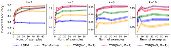
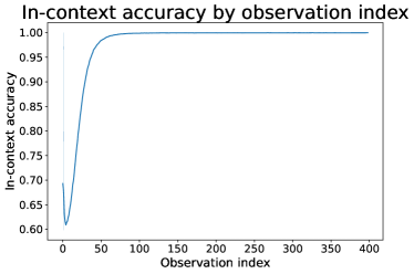
Results: Fig. 4[left] reports the in-context accuracy—defined as the average ratio of correct predictions—for each pair of the GINC test set. is outperformed by vanilla sequence models. However, outperforms both transformer and LSTM for all context lengths . For larger contexts , the best model is —it is however slower to converge (see Table 4, Appendix E). Finally, the highest in-context accuracies for TDB are around and are higher than what was reported in Xie et al. (2021) for transformers. The numerical values are in Table 8, Appendix K.
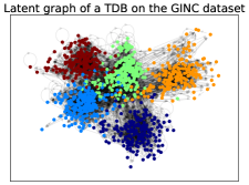
Fig. 4[right] displays the latent graph learned by TDB. We use and the Kamada-Kawai algorithm. Each latent node has a color corresponding to the GT concept with higher empirical frequency when this node is active. The learned latent graph has an interpretable structure: TDB learns five latent subgraphs corresponding to the five concepts in the GINC dataset.
 |
4.5 In-context learning experiments
Problem: Our last experiment explores whether vanilla models and TDB can, in a new test POE, (a) in-context predict the next observation (b) solve in-context path planning problems (c) learn in-context latent graphs. Similar to Sec.4.2, we first generate a D aliased room of size with unique colors, and with global aliasing: a patch is repeated twice. We define the room partition as the partition of the GT room spatial positions such that all the room spatial positions in a set have the same observation. We then generate many aliased rooms of the same size by preserving the room partition: each room picks colors out of without replacement, and assigns all the positions in to the same color. See Appendix L.1.
We train each model for a varying number of training rooms: 333That is, we train on at most of all the possible rooms.. The training set contains sequences: each sequence picks a training room at random, then generates a random walk of length in it. The test set only contains four random walks in each new test room. We define in-context path planning problems as before, using a context . Given a new test room, TDB derives the test bottleneck indices, builds an in-context cognitive map, and uses it to solve the in-context path planning problems.
Training in base: We map a sequence of observations in a room—where is one of the four room observations—to a room-agnostic sequence where (a) (b) iff. is the th lowest observation seen between indices and 444 may map to different through the sequence.. We train each model to take as input and to predict . Targets are always in the base , which encourages the models to share structure across rooms—e.g. TDB can reuse the same latent codes across rooms. As before, we train for k Adam iterations, using a learning rate of , a batch size of and a dropout of .
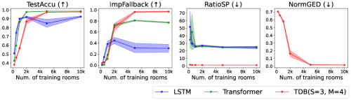
Results: Fig. 5[left] averages the results over runs—the numerical values are in Table 9, Appendix L.2. For NormGED, we use a timeout of . As the number of training rooms increases, all the models display a phase transition where both prediction and path planning performance improve. When the number of training rooms is larger than , in-context learning emerges for the transformer and TDB: both achieve almost perfect in-context accuracy on the new test rooms. In contrast, LSTM reaches lower in-context accuracy. In addition, in-context path planning emerges in the TDB: it can nearly perfectly solve the shortest paths problems, which both vanilla models struggle with. The in-context latent graphs reach low NormGED and are nearly isomorphic to the GT, and correctly model the room’s dynamics—see Fig. 5[right]. TDB trained on k rooms has a disentanglement accuracy (see Appendix F) of : again, multiple discrete bottlenecks do not learn a disentangled representation. Finally, Appendix L.4 studies how spatial exposure to base targets in the training data drives in-context performance.
5 Conclusion
We propose TDB, a transformer variant that addresses the shortcomings of vanilla transformers for path planning. TDB (a) introduces discrete bottlenecks which compress the information necessary to predict the next observation given history then (b) builds interpretable cognitive maps from the active bottlenecks indices. On perceptually aliased POEs, TDB (a) retains the near-perfect prediction of transformers, (b) calls an external solver on its latent graph to solve path planning problems exponentially faster, (c) learns interpretable structure from text datasets, (d) exhibits emergent in-context prediction and path planning abilities.
Our approach has two main limitations. First, TDB only accepts categorical inputs. Second, though multiple discrete bottlenecks accelerate training, they do not learn a disentangled latent space. To address these points, we want to modify the TDB architecture (a) to accept high-dimensional continuous observations (images) (b) so that different bottlenecks learn non-redundant representations. Furthermore, we would like to extend this work into a framework to build planning-compatible world models in rich environments. To do so, we want to learn disentangled latent dynamics in factored Markov decision processes by (a) extracting knowledge with transformers, (b) using multiple discrete bottlenecks to compress this knowledge and to generate latent nodes—or local latent graphs—and (c) learning factorized transition matrices over these latent nodes.
Acknowledgments
We thank Kevin Murphy, Daan Wierstra and Théophane Weber for useful discussions during the preparation of this manuscript.
References
- Beattie et al. (2016) Charles Beattie, Joel Z Leibo, Denis Teplyashin, Tom Ward, Marcus Wainwright, Heinrich Küttler, Andrew Lefrancq, Simon Green, Víctor Valdés, Amir Sadik, et al. Deepmind lab. arXiv preprint arXiv:1612.03801, 2016.
- Brown et al. (2020) Tom Brown, Benjamin Mann, Nick Ryder, Melanie Subbiah, Jared D Kaplan, Prafulla Dhariwal, Arvind Neelakantan, Pranav Shyam, Girish Sastry, Amanda Askell, et al. Language models are few-shot learners. Advances in neural information processing systems, 33:1877–1901, 2020.
- Carbonneau et al. (2020) Marc-André Carbonneau, Julian Zaidi, Jonathan Boilard, and Ghyslain Gagnon. Measuring disentanglement: A review of metrics. arXiv preprint arXiv:2012.09276, 2020.
- Chen et al. (2021a) Lili Chen, Kevin Lu, Aravind Rajeswaran, Kimin Lee, Aditya Grover, Misha Laskin, Pieter Abbeel, Aravind Srinivas, and Igor Mordatch. Decision transformer: Reinforcement learning via sequence modeling. Advances in neural information processing systems, 34:15084–15097, 2021a.
- Chen et al. (2021b) Mark Chen, Jerry Tworek, Heewoo Jun, Qiming Yuan, Henrique Ponde de Oliveira Pinto, Jared Kaplan, Harri Edwards, Yuri Burda, Nicholas Joseph, Greg Brockman, et al. Evaluating large language models trained on code. arXiv preprint arXiv:2107.03374, 2021b.
- Chowdhery et al. (2022) Aakanksha Chowdhery, Sharan Narang, Jacob Devlin, Maarten Bosma, Gaurav Mishra, Adam Roberts, Paul Barham, Hyung Won Chung, Charles Sutton, Sebastian Gehrmann, et al. Palm: Scaling language modeling with pathways. arXiv preprint arXiv:2204.02311, 2022.
- Chrisman (1992) Lonnie Chrisman. Reinforcement learning with perceptual aliasing: The perceptual distinctions approach. In AAAI, volume 1992, pages 183–188. Citeseer, 1992.
- Cobbe et al. (2021) Karl Cobbe, Vineet Kosaraju, Mohammad Bavarian, Mark Chen, Heewoo Jun, Lukasz Kaiser, Matthias Plappert, Jerry Tworek, Jacob Hilton, Reiichiro Nakano, et al. Training verifiers to solve math word problems. arXiv preprint arXiv:2110.14168, 2021.
- Conmy et al. (2023) Arthur Conmy, Augustine N Mavor-Parker, Aengus Lynch, Stefan Heimersheim, and Adrià Garriga-Alonso. Towards automated circuit discovery for mechanistic interpretability. arXiv preprint arXiv:2304.14997, 2023.
- Dai et al. (2019) Zihang Dai, Zhilin Yang, Yiming Yang, Jaime Carbonell, Quoc V Le, and Ruslan Salakhutdinov. Transformer-xl: Attentive language models beyond a fixed-length context. arXiv preprint arXiv:1901.02860, 2019.
- Dempster et al. (1977) Arthur P Dempster, Nan M Laird, and Donald B Rubin. Maximum likelihood from incomplete data via the em algorithm. Journal of the royal statistical society: series B (methodological), 39(1):1–22, 1977.
- Elhage et al. (2021) Nelson Elhage, Neel Nanda, Catherine Olsson, Tom Henighan, Nicholas Joseph, Ben Mann, Amanda Askell, Yuntao Bai, Anna Chen, Tom Conerly, et al. A mathematical framework for transformer circuits. Transformer Circuits Thread, 1, 2021.
- George et al. (2021) Dileep George, Rajeev V Rikhye, Nishad Gothoskar, J Swaroop Guntupalli, Antoine Dedieu, and Miguel Lázaro-Gredilla. Clone-structured graph representations enable flexible learning and vicarious evaluation of cognitive maps. Nature communications, 12(1):2392, 2021.
- Ghahramani and Jordan (1995) Zoubin Ghahramani and Michael Jordan. Factorial hidden markov models. Advances in Neural Information Processing Systems, 8, 1995.
- Grill et al. (2020) Jean-Bastien Grill, Florian Strub, Florent Altché, Corentin Tallec, Pierre Richemond, Elena Buchatskaya, Carl Doersch, Bernardo Avila Pires, Zhaohan Guo, Mohammad Gheshlaghi Azar, et al. Bootstrap your own latent-a new approach to self-supervised learning. Advances in neural information processing systems, 33:21271–21284, 2020.
- Guan et al. (2023) Lin Guan, Karthik Valmeekam, Sarath Sreedharan, and Subbarao Kambhampati. Leveraging pre-trained large language models to construct and utilize world models for model-based task planning. arXiv preprint arXiv:2305.14909, 2023.
- Guntupalli et al. (2023) J Swaroop Guntupalli, Rajkumar Vasudeva Raju, Shrinu Kushagra, Carter Wendelken, Danny Sawyer, Ishan Deshpande, Guangyao Zhou, Miguel Lázaro-Gredilla, and Dileep George. Graph schemas as abstractions for transfer learning, inference, and planning. arXiv preprint arXiv:2302.07350, 2023.
- Guo et al. (2022) Zhaohan Guo, Shantanu Thakoor, Miruna Pîslar, Bernardo Avila Pires, Florent Altché, Corentin Tallec, Alaa Saade, Daniele Calandriello, Jean-Bastien Grill, Yunhao Tang, et al. Byol-explore: Exploration by bootstrapped prediction. Advances in neural information processing systems, 35:31855–31870, 2022.
- Hagberg et al. (2008) Aric Hagberg, Pieter Swart, and Daniel S Chult. Exploring network structure, dynamics, and function using networkx. Technical report, Los Alamos National Lab.(LANL), Los Alamos, NM (United States), 2008.
- Hendrycks and Gimpel (2016) Dan Hendrycks and Kevin Gimpel. Gaussian error linear units (gelus). arXiv preprint arXiv:1606.08415, 2016.
- Hochreiter and Schmidhuber (1997) Sepp Hochreiter and Jürgen Schmidhuber. Long short-term memory. Neural computation, 9(8):1735–1780, 1997.
- Kamada et al. (1989) Tomihisa Kamada, Satoru Kawai, et al. An algorithm for drawing general undirected graphs. Information processing letters, 31(1):7–15, 1989.
- Kingma and Ba (2014) Diederik P Kingma and Jimmy Ba. Adam: A method for stochastic optimization. arXiv preprint arXiv:1412.6980, 2014.
- Lamb et al. (2022) Alex Lamb, Riashat Islam, Yonathan Efroni, Aniket Rajiv Didolkar, Dipendra Misra, Dylan J Foster, Lekan P Molu, Rajan Chari, Akshay Krishnamurthy, and John Langford. Guaranteed discovery of control-endogenous latent states with multi-step inverse models. Transactions on Machine Learning Research, 2022.
- Li et al. (2022) Kenneth Li, Aspen K Hopkins, David Bau, Fernanda Viégas, Hanspeter Pfister, and Martin Wattenberg. Emergent world representations: Exploring a sequence model trained on a synthetic task. arXiv preprint arXiv:2210.13382, 2022.
- Lieberum et al. (2023) Tom Lieberum, Matthew Rahtz, János Kramár, Geoffrey Irving, Rohin Shah, and Vladimir Mikulik. Does circuit analysis interpretability scale? evidence from multiple choice capabilities in chinchilla. arXiv preprint arXiv:2307.09458, 2023.
- Mialon et al. (2023) Grégoire Mialon, Clémentine Fourrier, Craig Swift, Thomas Wolf, Yann LeCun, and Thomas Scialom. Gaia: a benchmark for general ai assistants. arXiv preprint arXiv:2311.12983, 2023.
- Momennejad et al. (2023) Ida Momennejad, Hosein Hasanbeig, Felipe Vieira, Hiteshi Sharma, Robert Osazuwa Ness, Nebojsa Jojic, Hamid Palangi, and Jonathan Larson. Evaluating cognitive maps and planning in large language models with cogeval. arXiv preprint arXiv:2309.15129, 2023.
- Nanda et al. (2023) Neel Nanda, Lawrence Chan, Tom Liberum, Jess Smith, and Jacob Steinhardt. Progress measures for grokking via mechanistic interpretability. arXiv preprint arXiv:2301.05217, 2023.
- Olsson et al. (2022) Catherine Olsson, Nelson Elhage, Neel Nanda, Nicholas Joseph, Nova DasSarma, Tom Henighan, Ben Mann, Amanda Askell, Yuntao Bai, Anna Chen, et al. In-context learning and induction heads. arXiv preprint arXiv:2209.11895, 2022.
- Pallagani et al. (2022) Vishal Pallagani, Bharath Muppasani, Keerthiram Murugesan, Francesca Rossi, Lior Horesh, Biplav Srivastava, Francesco Fabiano, and Andrea Loreggia. Plansformer: Generating symbolic plans using transformers. arXiv preprint arXiv:2212.08681, 2022.
- Radford et al. (2018) Alec Radford, Karthik Narasimhan, Tim Salimans, Ilya Sutskever, et al. Improving language understanding by generative pre-training. 2018.
- Ramesh et al. (2021) Aditya Ramesh, Mikhail Pavlov, Gabriel Goh, Scott Gray, Chelsea Voss, Alec Radford, Mark Chen, and Ilya Sutskever. Zero-shot text-to-image generation. In International Conference on Machine Learning, pages 8821–8831. PMLR, 2021.
- Reed et al. (2022) Scott Reed, Konrad Zolna, Emilio Parisotto, Sergio Gomez Colmenarejo, Alexander Novikov, Gabriel Barth-Maron, Mai Gimenez, Yury Sulsky, Jackie Kay, Jost Tobias Springenberg, et al. A generalist agent. arXiv preprint arXiv:2205.06175, 2022.
- Sanfeliu and Fu (1983) Alberto Sanfeliu and King-Sun Fu. A distance measure between attributed relational graphs for pattern recognition. IEEE transactions on systems, man, and cybernetics, (3):353–362, 1983.
- Srivastava et al. (2022) Aarohi Srivastava, Abhinav Rastogi, Abhishek Rao, Abu Awal Md Shoeb, Abubakar Abid, Adam Fisch, Adam R Brown, Adam Santoro, Aditya Gupta, Adrià Garriga-Alonso, et al. Beyond the imitation game: Quantifying and extrapolating the capabilities of language models. arXiv preprint arXiv:2206.04615, 2022.
- Swaminathan et al. (2023) Sivaramakrishnan Swaminathan, Antoine Dedieu, Rajkumar Vasudeva Raju, Murray Shanahan, Miguel Lazaro-Gredilla, and Dileep George. Schema-learning and rebinding as mechanisms of in-context learning and emergence. arXiv preprint arXiv:2307.01201, 2023.
- Valmeekam et al. (2022) Karthik Valmeekam, Alberto Olmo, Sarath Sreedharan, and Subbarao Kambhampati. Large language models still can’t plan (a benchmark for llms on planning and reasoning about change). arXiv preprint arXiv:2206.10498, 2022.
- Van Den Oord et al. (2017) Aaron Van Den Oord, Oriol Vinyals, et al. Neural discrete representation learning. Advances in neural information processing systems, 30, 2017.
- Vaswani et al. (2017) Ashish Vaswani, Noam Shazeer, Niki Parmar, Jakob Uszkoreit, Llion Jones, Aidan N Gomez, Lukasz Kaiser, and Illia Polosukhin. Attention is all you need. Advances in neural information processing systems, 30, 2017.
- Wei et al. (2022) Jason Wei, Yi Tay, Rishi Bommasani, Colin Raffel, Barret Zoph, Sebastian Borgeaud, Dani Yogatama, Maarten Bosma, Denny Zhou, Donald Metzler, et al. Emergent abilities of large language models. arXiv preprint arXiv:2206.07682, 2022.
- Xie et al. (2021) Sang Michael Xie, Aditi Raghunathan, Percy Liang, and Tengyu Ma. An explanation of in-context learning as implicit bayesian inference. arXiv preprint arXiv:2111.02080, 2021.
Appendix A Vanilla transformer architecture
Fig.6 presents the vanilla transformer detailed in Sec.3.2. In our numerical experiments, Sec.4, we train this model to minimize the autoregressive objective Equation (1).
Appendix B On the connection between TDB and CSCG
B.1 Computational and space complexity
A clone-structured causal graph (CSCG) (George et al., 2021) is a hidden Markov model variant used to model sequences of categorical observations. The latent space of a CSCG is partitioned, such that all the latent variables in one set of the partition deterministically emit the same observation. These latent variables are the clones of the observation. Because of its latent structure, CSCG models a transition between two observations as a transition between their respective clones—as opposed to a transition between all the latent variables.
We compare below the complexity between a vanilla CSCG and a vanilla self-attention layer when running inference on a sequence of length .
Computation complexity: For a vanilla CSCG with clones per observation, the computational cost for computing the forward and backward messages is . In contrast, for a vanilla self-attention layer with a -dimensional embedding, the forward pass cost is . In this paper, we use , . CSCG is then more expensive when the number of clones per observation satisfies .
Space complexity: The memory cost of storing a vanilla CSCG with clones per observation and different observations is . This large dense memory matrix can grow quickly as the number of observations increases, and prohibit vanilla CSCGs from scaling to very large latent space. In contrast, a vanilla self-attention layer with a -dimensional embedding requires a memory. The quadratic dependence on the sequence length is problematic for large corpora, but not for the problem we study here, where .
B.2 A transformer with clone-structured discrete bottleneck
We propose herein a variant of the TDB architecture inspired by the CSCG model, which injects a “clone-structured” inductive bias into its discrete bottlenecks. We consider the dictionary of latent codes introduced in Sec.3.3: , where . We now allocate a subset of the latent codes for each observation in the vocabulary . That is, we first define a partition of the indices such that:
Second, we generalize the operator in Equation (2) so that it now depends on both (a) the transformer output and (b) the observation itself. That is, we define:
| (5) |
For the observation which leads to the transformer output , the discrete quantizer now returns the latent code of with index . That is, each observation can now only activate a subset of the latent codes. We refer to this new quantizer module as clone-structured discrete bottleneck.
Computational gain: This architecture change decreases the computational cost of the discrete bottleneck by a linear term —which can be of interest when the number of observations is large. However, the overall computational cost is still dominated by the quadratic cost of computing the attention matrices in the causal transformer.
Performance gain: Overall, we did not find any major benefit from replacing the discrete bottleneck of a TDB with its clone-structure variants. Our most promising result was that we were able to solve the D synthetic environments in Sec.4.3 using a single clone-structured discrete bottleneck—where a TDB needs more than one discrete bottleneck. However, a transformer with clone-structured bottlenecks would struggle to solve the in-context learning experiments in Sec.4.5. Indeed, a new test room with observations would, by definition, use different latent codes than a training room with observations , which prevents the model from learning to share structure across rooms. This convinced us to not use the clone-structured discrete bottleneck in our experiments.
Appendix C Clustering steps to build the transition graph
In this section, we detail the clustering steps that we apply to learn a cognitive map from the bottleneck indices in Sec.3.6.
Step 1. Cluster the bottlenecks indices with Hamming distance:
This first clustering step only applies in the case where the TDB has multiple discrete bottlenecks. In this case, TDB maps each observation to a tuple of latent code indices:
Before building the cognitive map, we first collect in a set all the unique tuples of latent indices appearing in the training set. For two tuples and , we compute their Hamming distance:
We introduce a distance threshold —which we set to in Sec.4—and merge any pair of tuples such that . This means that we will not distinguish and when we build the count tensor —see Sec.3.6. Consequently, these two tuples will be mapped to the same node on the cognitive map —and any node in will be associated with a collection of tuples of bottleneck indices.
Intuitively, this means that when the entries of two tuples of bottleneck indices are “almost all the same”, then we assume that their associated observations are at the same spatial position.
Step 2. Merge identical nodes:
Second, we build the count tensor (after this first clustering step), and threshold it with to build an action-augmented transition graph —as detailed in Sec. 3.6. We only retain nodes that have at least two incoming and outgoing neighbors. Finally, our second clustering step merges every pair of nodes in that are connected to the same set of neighbors.
Step 3. Map each discarded node to its closest retained node:
Thresholding the count tensor may discard some (tuple of) bottleneck indices with low empirical counts. In particular, as we show in Fig.10, Appendix I.3, many bottleneck indices that are active early in the sequences are discarded. This may be problematic for solving path planning problems, as it means that the corresponding observations cannot be mapped to nodes in . Indeed, when TDB activates a discarded (tuple of) bottleneck indices, it cannot locate itself in the learned cognitive map .
To remedy this, we divide the set of unique (tuples of) latent indices , between the elements that are discarded—i.e. not mapped to a node in —and retained—i.e. mapped to a node in . Our last clustering step maps any discarded (tuple of) latent indices to its closest retained latent index for the distance, defined as:
After this step, and are mapped to the same node in , and all the entries in are retained.
Appendix D Solving path planning problem at test time on partially observed environments
We detail herein how a vanilla sequence model and a TDB can solve the test shortest path problem presented in Sec.4.2.
Defining the shortest path problem:
We consider a test sequence of observations and actions in a POE—the environment can either be the D aliased rooms of Sec.4.2 and Sec.4.5, the aliased cube of Sec.4.2, or the egocentric D synthetic environments of Sec.4.3. We also denote the unobserved sequence of room spatial positions associated with each observation. Note that, because of aliasing, we cannot deterministically infer from .
For the D aliased rooms (Sec.4.2), the spatial position of an observation is its D coordinates. For the egocentric D synthetic environments (Sec.4.3), the spatial position of an observation is a D vector: the first two entries correspond to the D coordinates of the observation, while the last entry corresponds to the agent’s heading direction, which is one of
Let be a context length—we set or in practice. The path planning problem we consider in Sec.4 consists of finding the shortest path, i.e., the shortest sequence of actions, which leads from the room position (associated with the observation ) to the room position (associated with the observation ). Naturally, the sequence is a path of length from to , which we refer to as the fallback path. In addition, for evaluating a model’s performance, we use an optimal shortest path, which solves the shortest path problem in the ground truth room—note that the agent does not know the ground truth layout. While the optimal shortest path is not unique, all the optimal shortest paths have the same length.
Fig.1 in the main text illustrates this path planning problem on a D aliased room—we use for the sake of visualization.
We detail below our proposed procedure for solving this shortest path problem with a TDB; and with a vanilla transformer or a vanilla LSTM. As mentioned in the main text, a vanilla sequence model finds this challenging because (a) it can only perform forward rollouts—without being able to collapse redundant visitations of the same spatial position—and (b) it cannot tell whether it has reached its destination. In contrast, a TDB solves this problem by querying its learned latent graph.
We are interested in measuring (a) whether each model can derive a path that improves over the fallback path and (b) when a model derives such a better path, how much worse it is compared to the optimal shortest path.
Deriving shortest paths with TDB:
When TDB is evaluated on the test sequences and , it maps each observation to either (a) a single latent code index when we have a single discrete bottleneck or (b) a tuple of latent codes indices when we have multiple discrete bottlenecks.
As a reminder, each node in the learned cognitive map is associated with a collection of (tuples of) bottleneck indices—see Appendix C. However, the (tuples of) bottleneck indices and may not be associated with a node in . Consequently, we find two tuples of bottleneck indices and (a) with lowest Hamming distance from and and (b) which are associated with two nodes and in . Finally, we call the external networkx.shortest_path solver to find a shortest path between the nodes and .
Deriving shortest paths from rollouts with vanilla sequence models:
A naive option that finds the shortest path between and with a vanilla sequence model consists in exploring all the possible sequences of observations and actions. For a number of evaluations exponential in the length of the optimal shortest path, this approach is guaranteed to find an optimal shortest path.
We propose herein an alternative approach, which (a) is more computationally efficient, (b) is not guaranteed to find the optimal shortest path, and (c) in practice, often improves over the fallback path. Beforehand, let us define the subsequences of observations context and actions context . We also define the subsequences of observations tail and actions tail .
First, we generate random sequences of actions, each of length : we denote the th random sequence—we initialize the indices at . In Sec.4.3, we set .
Second, we augment each sequence of actions (of length ) into two sequences of observations and actions, of respective lengths and , as follows. The first observations and actions are the shared context and . The next actions correspond to . The corresponding sequence of observations corresponds to the sequence model’s autoregressive predictions. That is, for , we iteratively define as:
For each generated random walk, we look for all the observations equal to , and define the set of candidates:
Estimating whether the target is reached via tail evaluation:
As we mentioned in the main text, because of aliasing, the vanilla sequence model cannot know whether it has reached the target position when it observes a candidate. That is, it does not know whether the spatial position associated with the candidate is equal to .
We could return all the candidates and evaluate them using the ground truth map. Instead, we propose herein to estimate whether a candidate is at the target position by evaluating it—with its history—on the tail subsequences of observations and actions . That is, for a candidate we define, for :
We estimate that a candidate is at the target position when . Note that, because of aliasing, even when the tail evaluation succeeds, the candidate may not be at the target position.
Evaluating valid paths:
For the TDB, we return a single shortest path proposal, which is estimated by the external solver. For the transformer and the LSTM, we return all the path proposals that are estimated to be at the target position.
For each model, we first evaluate whether the proposed paths are valid. That is, we test whether the proposed sequence of actions correctly leads from to in the ground truth environment. For a vanilla sequence model, when multiple returned paths are valid, we only retain the shortest one. We then compute two metrics (a) a binary indicator of whether the method has found a valid path and (b) if (a) is correct, the ratio between the length of the valid found path and the optimal path length. Finally, ImpFallback averages (a) while RatioSP averages (b) over shortest paths problems.
Tail evaluation improves the quality of the paths returned:
For a transformer trained on D aliased rooms in Sec.4.2, if we return all the candidates, then the ratio of valid paths among the paths returned is . Indeed, most of the candidates are not at the target spatial position. When we estimate whether we are at the target position via tail evaluation, this ratio goes up to —prediction errors prevent it from being at . Similarly, on the D synthetic environments of Sec.4.3, a transformer without tail evaluation returns of valid paths while a transformer with tail evaluation returns . Finally, on the ICL experiments of Sec.4.5, for a transformer trained on rooms, this same ratio goes from without tail evaluation up to with it. Overall, tail evaluation drastically improves the quality of the paths returned by sequence models.
Appendix E Multiple discrete bottlenecks accelerate training
2D aliased rooms: For each TDB trained on the D aliased rooms and reported in Sec.4.2, we compute, for every training steps, its training accuracy on the entire training set. We define a new metric, TrainingAbove98, which reports the first evaluation when this training accuracy is higher than . Table 2 averages this metric over the experiments run in Sec.4.2, for various TDB models.
| Method | TrainingAbove98 |
|---|---|
| TDB | |
| TDB | |
| TDB | |
| TDB | |
| TDB | |
| TDB |
D synthetic environments: As discussed in Sec.4.2, we need discrete bottlenecks for the TDB training to converge in D synthetic environments. Table 3 illustrates this by reporting TrainingAfter1k—the training accuracy after training steps—for the different models reported in Table 7, Appendix J.
| Method | TrainingAfter1k |
|---|---|
| TDB | |
| TDB | |
| TDB | |
| TDB | |
| TDB | |
| TDB |
GINC text dataset: On the GINC dataset, we also evaluate the training accuracy of each model reported in Sec.4.5 at every training steps. Here, TrainingAbove98 reports the first iteration when the training accuracy becomes higher than of the highest value it reaches during training.
| Method | TrainingAfter1k |
|---|---|
| TDB | |
| TDB | |
| TDB | |
| TDB | |
| TDB | |
| TDB |
Appendix F Do multiple discrete bottlenecks learn a disentangled representation?
Predicting a discrete bottleneck index given the other indices:
We propose herein a metric to test whether multiple discrete bottlenecks learn a disentangled representation of the observations.
If the discrete bottlenecks learn of a disentangled representation, then (a) they have to be independent (b) each one has to explain a distinct factor of the data (Carbonneau et al., 2020). Given a TDB with discrete bottlenecks, we propose to estimate (a), that is, whether the bottlenecks are independent. To do so, we train a logistic regression estimator to predict each bottleneck index given the other bottleneck indices.
Given a sequence of observations , a TDB with discrete bottlenecks maps each observation to the latent codes where —see Sec.3.5.
We denote the one-hot encoding of .
Let us now assume that we want to predict the th bottleneck index given the first bottleneck indices.
We note and , where we drop the dependency over . We also introduce a matrix . The logistic regression objective at timestep is:
We also define . Note that we do not use an intercept term or a regularization term.
Training:
Given a training and test set from Sec.4, each consisting of test sequences of length , we first compute all the active bottleneck indices, which gives us two tensors, and , each of dimensions .
We train logistic regression estimators on : the th estimator is trained to minimize , that is, to predict the th bottleneck index given the other . For training, we use Adam (Kingma and Ba, 2014) for iterations, with a learning rate of and a batch size of .
Disentanglement metric:
Our proposed disentanglement metric is the averaged test accuracy of the logistic regression estimators on the test tensor .
Results:
In Sec.4, we use latent codes for each discrete bottleneck: if the bottleneck representations are independent, the test disentanglement accuracy would be . However, all the test disentanglement accuracies reported in the main paper, are above , which shows that multiple discrete bottlenecks learn highly redundant representations.
Appendix G TDB with single-step objective merges nodes with identical neighbors
In Sec.3.7, we make the argument that a TDB only trained to predict the next observation is not encouraged to disambiguate observations with identical neighbors in the ground truth (GT) room and, as a result, may merge their representations. We use this same argument in Sec.3.4 to justify the need for augmenting the loss via either (a) a multi-step objective or (b) next encoding prediction.
Fig.7 demonstrates the argument. We consider a D aliased GT room from Sec. 4.2 with unique observations—the numerical results are presented in Table 6, Appendix I.2. Similar to Fig.1, the GT room contains a patch with black borders repeated twice. Each patch contains an inner patch with fuchsia borders. For each node inside this inner patch, all four actions in the GT room (move up, down, left, and right) lead to the same neighbors, regardless of whether the node in the top-left patch or the bottom-right one.
Fig.7[right] shows the latent graph learned by a TDB with single step prediction and four discrete bottlenecks. Because this model is only trained to predict the next observation given the history, it learns the same representation for each pair of nodes with same location inside the inner patch. This results in the presence of four merged nodes in the latent graph—colored in fuchsia. When a merged node is active, the agent can (a) perfectly predict the next observation but (b) it cannot know which one of the two possible patches it is in. In addition, the merged nodes introduce unrealistic shortcuts in the learned latent graph: nodes that are far apart in the GT room are close in the latent graph. Because the learned cognitive map does not accurately model the ground truth dynamics, the external solver will propose shortest paths that are invalid in the GT room. As a consequence, as indicated in Table 6, Appendix I.2, TDB can only solve of the path planning problems.
For aliased rooms with 4 colors: When , a higher frequency of observations have identical neighbors. The learned latent graph merges these observations, which introduces a larger number of unrealistic shortcuts. This explains the poor performance of TDB() in Table 1, which only improves of the time over the fallback path. Because of this inherent model failure, TDB() similarly only improves over the fallback path of the time. In fact, TDB is only able to solve the easiest path planning problems, for which the optimal shortest path consists of only a small number of actions. Indeed, the average length of the optimal shortest paths solved by TDB() is while the average length of the optimal shortest paths over all the path planning problems is .
For 3D synthetic environments: Fig.8[middle] shows that, for a D environment from Section 4.3, the cognitive map learned with a TDB merges three pairs of nodes. These merged nodes introduce unrealistic shortcuts on the learned latent graph: as a result, TDB fails at path planning and only improves of the time over the fallback path.
Fig.8[right] shows the latent graph learned when the objective is augmented to predict the next three steps, and highlights the three pairs of nodes merged in the middle image. Note that each node is mapped to the observation with higher empirical frequency when this node is active. As before, we see that the merged nodes have identical neighbors555Because there are clusters, the reader cannot precisely infer the observation from the colors: we looked at the graph indices to make sure that the neighbors of the merged nodes are identical..

Appendix H Accelerating the graph edit distance
The graph edit distance (GED) (Sanfeliu and Fu, 1983) between two graphs and is a graph similarity measure defined as minimum cost of edit path—i.e. sequence of node and edge edit operations—to transform the graph into a graph isomorphic to .
Computing the exact GED is NP-complete.
We therefore rely on the networkx.optimize_graph_edit_distance (Hagberg et al., 2008) function to return a sequence of approximations. This method accepts as argument a function to indicate which nodes (resp. edges) of and should be considered equal during matching.
To accelerate GED, we say that a node of and a node of have to be considered equal — and we note if the ground truth spatial positions with higher empirical frequency when (resp. ) is active are the same. Similarly, we say that an edge of connecting the nodes and an edge of connecting the nodes are considered to be equal if either (a) and or (b) and .
We use a timeout of s to compute GED in all the experiments but the ICL one, for which we use s (due to the large number of normalized graph edit distances being computed).
Appendix I Additional materials for aliased cube and for D aliased room cubes
I.1 Table of results for non-Euclidean aliased cube
Table 6 reports the prediction and path planning metrics for an aliased cube with edge size , similar to Fig. 3[bottom-left]. All the settings and parameters are the same as in Section 4.2. We average the results over experiments: each experiment considers a different cube.
| Method | TestAccu () | ImpFallback () | RatioSP | NormGED |
|---|---|---|---|---|
| Vanilla transformer | — | |||
| Vanilla LSTM | — | |||
| TDB | ||||
| TDB |
I.2 Table of results for 12 unique observations
Table 6 reports the prediction and path planning metrics for an aliased room with unique observations and global aliasing—as a patch is repeated twice. All the settings and parameters are the same as in Section 4.2.
First, during training, a TDB with a single discrete bottleneck either (a) is stuck in a local optimum or (b) converges after a long time. As a consequence, contrary to Table 6 which considers , all the TDBs with a single bottleneck are here outperformed by their counterparts with four bottlenecks. TDBs with a single bottleneck also learn worse cognitive maps and solve a lower frequency of path planning problems.
Second, regardless of the number of bottleneck used, a TDB with single-step objective cannot disambiguate the global aliasing and introduces unrealistic shortcuts—see Appendix G—which result in a drop in planning metrics.
In contrast, TDBs with bottlenecks and either multi-step or next encoding objective (a) achieves nearly perfect prediction accuracy, (b) are able to almost consistently find the optimal shortest path, and (c) learn cognitive maps that recover the GT dynamics.
| Method | TestAccu () | ImpFallback () | RatioSP | NormGED |
|---|---|---|---|---|
| Vanilla transformer | — | |||
| Vanilla LSTM | — | |||
| TDB | ||||
| TDB | ||||
| TDB | ||||
| TDB | ||||
| TDB | ||||
| TDB |
I.3 The agent can locate itself after a short context
Test accuracy by timestep:
Fig.9 shows the average prediction accuracy as a function of the observation index for our best TDB, reported in Sec.4.2 for the D aliased room with observations.
Because of aliasing, at the start of a test random walk, the model cannot know its location in the D room: the prediction accuracy for the first timesteps is low. The agent then quickly locates itself and test accuracy rapidly increases: it is above after only observations.
Some latent codes model early uncertainty while others represent late confidence: Fig.10 displays, for each latent code active on the test data of a TDB (a) the average timestep at which this latent code is active—on the horizontal axis—and (b) its number of appearances on the entire test data—on the vertical axis. In addition, each bottleneck is colored in green (resp. red) to indicate that it is retained (resp. discarded) when we threshold the empirical count tensor to build the cognitive map—as detailed in Sec.3.6.

The figure displays two clusters, which highlight the two roles played by the latent codes. The first cluster represents a large number of codes with low appearance counts, which appear early in the test sequences. These codes model the agent’s uncertainty when it does not know its location.
The latent codes in the second cluster have a high number of appearances and appear later in the test sequences. They represent the agent’s high confidence when it knows its locations. In addition, because we use a high count threshold (see Sec.3.6) to build the cognitive map, only the transitions between the latent codes of this second cluster are used to build the graph. As a result, a vast majority of the nodes of the second (resp. first) cluster are green (resp. red). Consequently, our third clustering step, detailed in Appendix C, maps the discarded (red) latent indices to their closest retained (green) latent index.
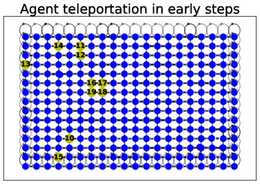
The agent can “teleportate”: We finally study how TDB moves in the learned latent graph. In particular, we say that the agent “teleportates” when the node of the transition graph where it estimates its location at the th timestep is not a neighbor of its estimated position at the th timestep. That is, teleportation means that the shortest path between two consecutive nodes is larger than one.
Fig.11 looks at the average number of teleportation as a function of the observation index. Around the th observation, the agent still teleportates of the time. As the agent becomes confident about its location, the teleportation rate drops below after observations and stays around .
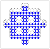
Interestingly, Fig.9[right] shows a subsequence of observations on a test random walks, with perfect next observation accuracy. Nonetheless, the agent still “teleportates” five times out of ten.
Here, teleportation is an artifact of the clustering procedures that we use when we build the cognitive map—see Appendix. C. For instance, our third clustering step may incorrectly map some discarded bottleneck indices to their closest bottleneck index. As a consequence, when the agent activates a discarded bottleneck index, it may be mapped to an invalid room location. If we use a lower threshold , then teleportations should disappear but the learned latent graph would not accurately model the environment’s dynamics.
Appendix J Additional materials for simulated 3D environment
Table of results:
We first present the table of results for the simulated D environment experiments in Sec.4.3.
| Method | TestAccu () | ImpFallback () | RatioSP | NormGED |
|---|---|---|---|---|
| Vanilla transformer | — | |||
| Vanilla LSTM | — | |||
| TDB | ||||
| TDB | ||||
| TDB | ||||
| TDB |
Latent graphs visualizations:
Second, Fig.12 presents the isometric views of four D simulated rooms, as well as the respective cognitive maps learned with a TDB().

Appendix K Additional materials for GINC dataset
| Context length | Num. of examples | LSTM | Transformer | TDB | TDB |
|---|---|---|---|---|---|
Appendix L Additional materials for in-context learning
L.1 Defining the in-context learning problem
Preserving the room partition:
We consider a first D aliased room of size with observations, such that . We represent this room by a matrix , where, for and , is the room observation at the spatial position .
We define the room partition induced by the room colors as the partition of the D room spatial positions such that, for each element of the partition, all the spatial positions in have the same observation.
Formally, the room partition is defined as
and satisfies
For each injective mapping , we can build a new room with (a) observations and which (b) preserves the room partition, by assigning all the D spatial positions in to the observation . That is
The training sets in Sec.4.5 contain at most k such training rooms, each one preserving the room partition. Note that, for a given partition, the number of possible rooms which preserves the room partition is the number of injective mapping from to , which is .
Learning in base:
As discussed in the main text, given a sequence of observations in a room defined as above, each model is trained to predict targets in the room-agnostic base, , such that iff. is the th lowest observation seen between indices and .
In particular, let us define the permutation of such that . Let be such a large enough integer such that all the different room observations have been seen between and . Then, for , the target corresponds to the th highest color of the room, which is equal to .
L.2 Table of results
| Metric | Num. training rooms | LSTM | Transformer | TDB | TDB |
|---|---|---|---|---|---|
| TestAccu () | |||||
| ImpFallback () | |||||
| RatioSP | |||||
| NormGED | — | — | |||
| — | — | ||||
| — | — | ||||
| — | — | ||||
| — | — | ||||
| — | — |
First, we observe that for each model, in-context capacities emerge when we increase the number of rooms.
Second, while vanilla LSTM performs best for a small number of training rooms, it cannot reach near-perfect in-context accuracies when the number of training rooms increases—which a vanilla transformer can do. We believe that attention-like mechanisms are important for in-context capacities to fully emerge in novel test rooms.
Third, as observed in other experiments, vanilla sequence models cannot solve path planning problems. Indeed, for a large number of training rooms, a transformer improves at best of the times over the fallback path. However, when it does so, it finds paths that are on average times longer than the optimal paths. In contrast, our best TDB (a) almost matches the nearly perfect in-context predictive performance of a vanilla transformer, (b) almost perfectly solves in-context path planning problems and (c) learns in-context latent graphs nearly isomorphic to the ground truth.
Finally, our TDB—which also predicts the next latent encoding—performs worse than the other models. This is explained by its large variances across the different experiments. In fact, we observe that for two out of ten experiments, its training accuracy remains very low—below —as the model struggles to learn to predict the next observation. For the remaining eight runs, prediction and path planning performance are near optimal and the model competes with our best TDB. We could try increasing the number of bottlenecks and training a TDB to mitigate this issue.
L.3 In-context accuracy by timestep
Fig.13 shows the average in-context accuracy on the new test rooms, as a function of the observation index, for our best TDB trained on k rooms. Interestingly, in-context accuracy drops after a few iterations. Indeed, as the model sees new observations in the new test rooms, the mapping between the base labels and the observations may change—which may confuse the model. After a few tenths of iterations, TDB is able to locate itself in the new test room. After iterations, in-context accuracy becomes higher than .
L.4 In-context learning is driven by spatial exposure to base targets in the training data
Restricting training rooms: For this experiment, we build training rooms such that the th highest color (almost) never appears at any of the spatial positions indicated by the set of the room partition. With the notations of Appendix L.1, each injective mapping used to generate a training room has to satisfy the rule
For instance, the mapping cannot be used to generate a training room. Indeed, when we rank the entries we get and violates . Similarly violates as .
Given a training sequence , let be such a large enough integer such that all the different room observations have been seen between and . For , let be such that the spatial position of the agent at timestep belongs to the set of the room partition. Then, by definition, the base target satisfies . Note that, by definition, when and we have not yet observed all the different room observations, we may have when .
Consequently, for each room spatial position, there is a position-specific base target that the agent will never see (when ) at this position on the training set.
We generate k such training rooms and train a TDB as before.
In-context accuracies:
We consider four families of test rooms:
(A): Test rooms where is respected.
(B): Test rooms where is violated once.
(C): Test rooms where is violated twice.
(D): Test rooms where is violated four times. These are the rooms satisfying .
On test rooms (A), in-context accuracy is .
On test rooms (B), in-context accuracy is .
On test rooms (C), in-context accuracy is .
On test rooms (D), in-context accuracy is .
This drastic drop in in-context accuracy demonstrates that—in addition to the number of training rooms—in-context capacities are also driven by spatial exposure to base targets during training.