Lecture notes on Malliavin calculus in regularity structures

Abstract.

Malliavin calculus provides a characterization of the centered model in regularity structures that is stable under removing the small-scale cut-off. In conjunction with a spectral gap inequality, it yields the stochastic estimates of the model.

This becomes transparent on the level of a notion of model that parameterizes the solution manifold, and thus is indexed by multi-indices rather than trees, and which allows for a more geometric than combinatorial perspective. In these lecture notes, this is carried out for a PDE with heat operator, a cubic nonlinearity, and driven by additive noise, reminiscent of the stochastic quantization of the Euclidean $\phi^{4}$ model.

More precisely, we informally motivate our notion of the model $(\Pi,\Gamma)$ as charts and transition maps, respectively, of the nonlinear solution manifold. These geometric objects are algebrized in terms of formal power series, and their algebra automorphisms. We will assimilate the directional Malliavin derivative to a tangent vector of the solution manifold. This means that it can be treated as a modelled distribution, thereby connecting stochastic model estimates to pathwise solution theory, with its analytic tools of reconstruction and integration. We unroll an inductive calculus that in an automated way applies to the full subcritical regime.

MSC 2020: 60H17, 60L30, 60H07, 81T16.

1. Motivation and setting

1.1. A nonlinear partial differential equation for $\phi$ with rough right-hand side $\xi$

We focus on the parabolic differential operator of second order (in fact, the heat operator) in $d$ space dimensions

$$L:=\partial_{0}-\sum_{i=1}^{d}\partial_{i}^{2},$$

where $\partial_{i}$ denotes the partial derivative w. r. t. $x_{i}$. Hence $x_{0}$ is the time-like variable and $\{x_{i}\}_{i=1}^{d}$ are the space-like variables. Given a parameter $\lambda$ and a space-time function $\xi$ we are interested in the manifold of all space-time functions $\phi$ that solve the partial differential equation (PDE) in the entire space-time

(1) $$L\phi-\lambda\phi^{3}=\xi\quad\mbox{on}\;\mathbb{R}^{1+d},$$

which is nonlinear due to the presence of the cube. At this point, let us emphasize that our use of the word “manifold” throughout these notes is informal. In particular, we will not attempt to rigorously endow the space of solutions to (1) with the structure of a topological manifold.

We are interested in the situation when the right-hand side (r. h. s.) $\xi$ is so rough that it is not a function but just a Schwartz distribution. A Schwartz distribution $\xi$ is a bounded linear form on the space of Schwartz functions. The space of Schwartz functions in turn is the linear space of all infinitely often differentiable functions $\zeta$ that decay so fast that the family of semi-norms

(2) $$\sup_{x\in\mathbb{R}^{1+d}}(|x|^{k}+1)|\partial^{\bf n}\zeta(x)|\quad\mbox{is finite},$$

where $k\in\mathbb{N}_{0}$, ${\bf n}=(n_{0},\cdots,n_{d})\in\mathbb{N}_{0}^{1+d}$, and $\partial^{\bf n}$ $:=\prod_{i=0}^{d}\partial_{i}^{n_{i}}$. The pairing is denoted by $(\xi,\zeta)$.

A pertinent example for $d=0$ is the following: Take a realization of Brownian motion, which we think of as a function $B_{x_{0}}$ of our time-like variable $x_{0}$, and consider

(3) $$(\xi,\zeta)=-\int_{\mathbb{R}}dx_{0}B_{x_{0}}\partial_{0}\zeta.$$

Since by the law of the iterated logarithm (i. e. $|B_{x_{0}}|\lesssim|x_{0}|^{\alpha}+1$ for any $\alpha>\frac{1}{2}$) we have $|(\xi,\zeta)|$ $\lesssim\sup_{x}(|x|^{2}+1)|\partial_{0}\zeta(x)|$, $\xi$ is indeed a Schwartz distribution. Informally, i. e. in a distributional sense, one writes (3) as $\xi=\partial_{0}B$. The derivative $\xi$ of Brownian motion is called (temporal) white noise. Note that $\phi=B$ satisfies (1) with $\lambda=0$ (next to $d=0$). Since almost surely, $B$ has infinite variation, $\xi$ cannot be represented as an integral against a locally integrable function, and thus is a genuine Schwartz distribution.

We are interested in the even worse situation when solutions $\Pi_{0}$ of the corresponding linear problem, i. e. (1) with $\lambda=0$,

(4) $$L\Pi_{0}=\xi$$

are genuine Schwartz distributions. If $\Pi_{0}$ and $\xi$ are distributions, (4) is to be interpreted in the sense of

(5) $$(\Pi_{0},L^{*}\zeta)=(\xi,\zeta)\quad\mbox{for all Schwartz functions $\zeta$},$$

where $L^{*}:=-\partial_{0}-\sum_{i=1}^{d}\partial_{i}^{2}$ is the (informal) dual of $L$. Once more, $d=0$ provides an easy example: if $\xi=\frac{d^{2}B}{dx_{0}^{2}}$ then $\Pi_{0}=\frac{dB}{dx_{0}}$ modulo an additive random constant, and thus is a genuine distribution.

However, if $\Pi_{0}$ is a genuine distribution, then its cube $\Pi_{0}^{3}$ does not have a canonical sense, which is why the equation is called “singular” in this regime. This does not bode well for the non-linear problem (1) and is the challenge addressed in these lecture notes.

1.2. Structure of these lecture notes

In Section 1 we informally motivate and rigorously introduce our version of a centered model in the language of regularity structures. In doing so, we adopt a more geometric than combinatorial perspective. In Subsection 1.5, we postulate the form of a counter term for (1), motivated by the symmetries from Subsection 1.4. We then introduce the concept of a parameterization of the nonlinear solution manifold (Subsection 1.6), informally write it as a power series (Subsection 1.7) giving rise to the index set of multi-indices, and finally “algebrize” it in terms of a formal power series $\Pi$ (Subsection 1.8), with $\Pi^{-}$ and $c$ corresponding to the r. h. s. and the counter term, respectively.

In the following subsections, we rigorously characterize $(\Pi,\Pi^{-},c)$: Only some of the coefficients are allowed to be non-zero, i. e. “populated” (Subsection 1.9). Returning to the scale invariance of the solution manifold (Subsection 1.10), we introduce the “homogeneity” of a multi-index (Subsection 1.11), and impose a scaling invariance on the coefficients of $(\Pi,\Pi^{-},c)$. Restricting to the singular but renormalizable range (Subsection 1.13), and as a consequence of a Liouville principle, $\Pi$ is unique (Subsection 1.12), and $c$ and thus $\Pi^{-}$ are unique (Subsection 1.14); the latter connects to what is called BPHZ renormalization.

However, by imposing the scale invariance, we arbitrarily singled out an origin; we now consider an arbitrary “base point” $x$. This gives rise to another parameterization $\Pi_{x}$ (Subsection 1.15), and thus to a change-of-basepoint transformation $\Gamma_{x}^{*}$ (Subsection 1.16), which is algebrized as an endomorphism of the algebra of formal power series. The following subsections deal with the structure of $\Gamma_{x}^{*}$ and its pre-dual $\Gamma_{x}$: its uniqueness (Subsection 1.19), its action on space-time polynomials (Subsection 1.17), its matrix representation (Subsection 1.18), the population of its matrix entries (Subsection 1.20), and its triangularity (Subsection 1.21). All this amounts to a self-contained introduction of a centered model $(\Pi_{x},\Pi_{x}^{-},\Gamma_{xx^{\prime}}:=\Gamma_{x}\Gamma_{x^{\prime}}^{-1})$ in the sense of regularity structures.

In Section 2, we state the stochastic estimates on $(\Pi_{x},\Pi_{x}^{-},\Gamma_{x})$ and sketch their proof, focussing here on the algebraic aspects. The scale invariance in law that emerges in the limit of vanishing regularization motivates the uniform estimates (Subsection 2.1). The main result and some extensions are formulated in Subsections 2.2 and 2.3. The motivation for the usage of the (directional) Malliavin derivative $\delta\Pi$ is given in Subsection 2.4. Its control requires a further structural insight, arising from the (informal) parameterization of the tangent space to the solution manifold, see Subsection 2.5. This motivates to approximate $\delta\Pi$, locally near $x$, by a linear combination of $\Pi_{x}$, with coefficients encoded in a linear endomorphism ${\rm d}\Gamma_{x}^{*}$. The latter can be assimilated with a modelled distribution in the language of regularity structures. The next subsections are devoted to the structure of ${\rm d}\Gamma_{x}^{*}$: its uniqueness (Subsection 2.7), the population of its matrix entries (Subsection 2.9), and its triangularity (Subsection 2.10), which determines the order of induction in the proof. While the original relation $\Pi\mapsto\Pi^{-}$ is not robust under vanishing regularization, its counterpart $\delta\Pi\mapsto\delta\Pi^{-}$ on the level of Malliavin derivatives is (Subsection 2.8).

In the following subsections we embark on the actual (stochastic) estimates: In Subsection 2.11, we introduce our use of the spectral gap inequality by duality, estimating probabilistic $L^{p}$-norms. The carré-du-champs is inherently linked to the space-time $L^{2}$ topology; this is best propagated by working with $L^{2}$-based space-time Besov norms (Subsection 2.12). We then lay out the induction step, which is a sequence of four arguments: a continuity property of $x\mapsto{\rm d}\Gamma_{x}^{*}$, namely an estimate of ${\rm d}\Gamma_{x+y}^{*}-{\rm d}\Gamma_{x}^{*}\Gamma_{x\,x+y}^{*}$, by an algebraic argument (Subsection 2.13), an estimate of the “rough-path increment” $\delta\Pi^{-}-{\rm d}\Gamma_{x}^{*}\Pi_{x}^{-}$ by what in regularity structures corresponds to a reconstruction of $\delta\Pi^{-}$ (Subsection 2.14), an estimate of $\delta\Pi-{\rm d}\Gamma_{x}^{*}\Pi_{x}$ by Schauder theory which in regularity structures is called integration (Subsection 2.15), and returning to the continuity property of $x\mapsto{\rm d}\Gamma_{x}^{*}$ by an analytic argument we call three-point argument (Subsection 2.16).

This is the crucial but only the first of three rounds of these four arguments, as explained in Subsection 2.17: What was done for $(\delta\Pi$ $-{\rm d}\Gamma_{x}^{*}\Pi_{x},$ $\delta\Pi^{-}-{\rm d}\Gamma_{x}^{*}\Pi_{x}^{-},$ ${\rm d}\Gamma_{x+y}^{*}-{\rm d}\Gamma_{x}^{*}\Gamma_{x\,x+y}^{*})$ needs to be repeated for $(\delta\Pi,\delta\Pi^{-},{\rm d}\Gamma_{x}^{*})$ (Subsection 2.18), and finally for $(\Pi,\Pi^{-},\Gamma_{x}^{*})$ itself (Subsection 2.19). The arguments in the second and third round, which have to carried out within the induction step in the right order, are simpler.

In Section 3, we provide the analytical details of the proof. A family of convolution operators that has the semi-group property (Subsection 3.1) is convenient, as it allows for telescoping over dyadic space-time scales in reconstruction (Subsection 3.2). It is also convenient when passing from an estimate of $\delta\Pi^{-}-{\rm d}\Gamma_{x}^{*}\Pi_{x}^{-}$ to one of $\delta\Pi^{-}$ (Subsection 3.3), and when estimating the expectation $\mathbb{E}\Pi^{-}$ (Subsection 3.4). Any general Schwartz convolution kernel can be recovered (Subsection 3.5). The last two subsections deal with integration, where the semi-group convolution now provides a decomposition of $L^{-1}$ into small and large scales, which is quintessential for any Schauder theory. Subsection 3.6 deals with the simpler cases of $\Pi$ and $\delta\Pi$; Subsection 3.7 tackles the more complex case of $\delta\Pi-{\rm d}\Gamma^{*}_{x}\Pi_{x}$, which involves an intermediate range of scales.

Contents

1. 1 Motivation and setting
   1. 1.1 A nonlinear partial differential equation for $\phi$ with rough right-hand side $\xi$
   2. 1.2 Structure of these lecture notes
   3. 1.3 Bibliographical context
   4. 1.4 A random $\xi$ with symmetries in law
   5. 1.5 Renormalization through a counter term $h$
   6. 1.6 Parameterization $(\lambda,p)\mapsto(h,\phi)$ of the solution manifold
   7. 1.7 Multi-indices $\beta$ and power series representation $\{\Pi_{\beta},c_{\beta}\}_{\beta}$ of the parameterization
   8. 1.8 Characterization of $\Pi$ and $\Pi^{-}$ as formal power series
   9. 1.9 Noise homogeneity $[\cdot]+1$ and population conditions on $\Pi,\Pi^{-}$
   10. 1.10 A scale invariance of noise and solution manifold
   11. 1.11 The homogeneity $|\cdot|$
   12. 1.12 Uniqueness of $\Pi_{\beta}$ given $\Pi_{\beta}^{-}$
   13. 1.13 Restriction to the singular and subcritical range $\alpha\in(-1,0)$
   14. 1.14 Uniqueness of $c$ via BPHZ choice of renormalization
   15. 1.15 Shift-invariance of the solution manifold, general base-points $x$, and corresponding $\Pi_{x}$
   16. 1.16 The change-of-base-point transformation $\Gamma_{x}^{*}$
   17. 1.17 $\Gamma_{x}$ acts by shift on space-time polynomials
   18. 1.18 Matrix representation $\{(\Gamma_{x}^{*})_{\beta}^{\gamma}\}$ of $\Gamma_{x}^{*}$
   19. 1.19 Uniqueness of $\Gamma_{x}$ given $\Pi$ and $\Pi^{-}$
   20. 1.20 Population of $\Gamma_{x}^{*}$
   21. 1.21 Strict triangularity of $\Gamma_{x}^{*}$
2. 2 Main result and sketch of proof
   1. 2.1 What estimates to expect?
   2. 2.2 Statement of main result
   3. 2.3 Population of $\Gamma^{*}$ and estimates of $\Pi_{\beta}$ for $\beta=\delta_{3}+\delta_{\bf 0},2\delta_{3}+\delta_{\bf 0}$ revisited
   4. 2.4 Usage of the (directional) Malliavin derivative $\delta$, first attempt
   5. 2.5 Tangent space to solution manifold
   6. 2.6 Modelling the Malliavin derivative $\delta\Pi$ by ${\rm d}\Gamma_{x}^{*}$
   7. 2.7 Uniqueness of ${\rm d}\Gamma_{x}^{*}$
   8. 2.8 A robust relation $\delta\Pi\mapsto\delta\Pi^{-}$
   9. 2.9 Population of ${\rm d}\Gamma_{x}^{*}$
   10. 2.10 Strict triangularity of ${\rm d}\Gamma_{x}^{*}$, order $\prec$ of induction
   11. 2.11 Usage of the spectral gap inequality
   12. 2.12 Besov-type norms and base case
   13. 2.13 The algebraic argument for ${\rm d}\Gamma_{x+y}^{*}-{\rm d}\Gamma_{x}^{*}\Gamma_{x\,x+y}^{*}$
   14. 2.14 Reconstruction for $\delta\Pi^{-}-{\rm d}\Gamma_{x}^{*}\Pi_{x}^{-}$
   15. 2.15 Integration for $\delta\Pi-{\rm d}\Gamma_{x}^{*}\Pi_{x}$
   16. 2.16 The three-point argument for ${\rm d}\Gamma_{x+y}^{*}-{\rm d}\Gamma_{x}^{*}\Gamma_{x\,x+y}^{*}$
   17. 2.17 Logical order of the proof
   18. 2.18 A second round of algebraic argument, reconstruction, integration, and three-point argument to estimate $(\delta\Pi,\delta\Pi^{-},$ ${\rm d}\Gamma^{*})$
   19. 2.19 A third round of algebraic argument, reconstruction, integration, and three-point argument to estimate $(\Pi,\Pi^{-},\Gamma^{*})$
3. 3 Proof details
   1. 3.1 Semi-group convolution
   2. 3.2 Details on reconstruction for $\delta\Pi^{-}-{\rm d}\Gamma_{x}^{*}\Pi_{x}^{-}$
   3. 3.3 Details on reconstruction for $\delta\Pi^{-}$
   4. 3.4 Details on the expectation $\mathbb{E}\Pi_{\beta t}^{-}(0)$ for $|\beta|<2$
   5. 3.5 Change of kernel
   6. 3.6 Details on integration for $\Pi$ and $\delta\Pi$
   7. 3.7 Details on integration for $\delta\Pi-{\rm d}\Gamma_{x}^{*}\Pi_{x}$

1.3. Bibliographical context

The theory of regularity structures [Hai14] provides a systematic framework to treat equations in a singular regime as outlined in Subsection 1.1. Inspired by rough path theory [Lyo98, Gub04], it separates analytic from probabilistic arguments, the former being dealt with in [Hai14] while the latter is addressed in [CH16]. In addition it comes with an algebraic structure [BHZ19, BCCH21], which allows to treat equations arbitrarily close to criticality. For an introduction to regularity structures we recommend [Hai15]; more focus on the algebraic aspects is put in [Che22a]. While the above-mentioned works provide a local well-posedness theory for a large class of singular stochastic PDEs, this setting can also be leveraged to establish global well-posedness results [CMW23] and to prove properties of the associated invariant measure [HS22]. Some of the most recent developments include progress on the stochastic quantization of the two and three dimensional Yang-Mills measure [CCHS22a, CCHS22b, CS23], for an overview see [Che22b].

Like [OST23], these lecture notes are intended as a reader’s digest of [LOTT21]. The present notes give a more complete account of [LOTT21] than the older notes [OST23], however adapted to a different model case, namely the semi-linear $\phi^{4}$ equation rather than the previously treated quasi-linear equation, thus confirming the flexibility of the approach, see also [BL23, GT23]. In the analytic treatment, these notes adopt a simplification from the recent [HS23] (see the discussion around (2.13) below) which in turn took inspiration from [LOTT21].

Loosely speaking, [LOTT21] constitutes an alternative to [CH16] when it comes to establishing the stochastic estimate of the centered model in regularity structures. The approach of [LOTT21] is based on Malliavin calculus in conjunction with a spectral gap estimate, and was taken over in [HS23]. Following [LOTT21], but opposed to [HS23], these lecture notes implement this approach for a model that can be seen as a parameterization of the solution manifold, a top-down approach that leads to a more parsimonious index set than trees, namely multi-indices. This type of model was introduced in [OSSW21], and then motivated in [LO22] in a non-singular setting. Building upon [OST23], we highlight the conceptual use of Malliavin calculus, which is brought to full fruition in [Tem23].

We note that prior to this line of research, Malliavin calculus had been used within regularity structures, but with a more classical purpose, namely the study of densities of solutions to stochastic partial differential equations, see [CFG17, GL20, Sch23]. Stochastic estimates based on a spectral gap assumption were first carried out in [IORT23], however in a simple setting with no need of regularity structures. More recently, and inspired by [LOTT21], the spectral gap inequality has been adopted as a convenient tool to prove stochastic estimates in regularity structures: in the tree-setting but without appealing to diagrams in [HS23, BH23], in the tree-setting and making use of diagrammatic tools in [BB23], and in a rough path setting in [GK23].

The (pre-)Lie- and Hopf-algebraic aspects of the structure group of this multi-index based model were first explored in [LOT23], and embedded into a post-Lie perspective in [BK23, JZ23]. In [BD23] it was shown that the algebraic structure on multi-indices is also a multi-Novikov algebra, which is isomorphic to the free multi-Novikov algebra. Some algebraic aspects of renormalization in the multi-index setting are investigated in [BL23], and the analogue for rough paths is studied in [Lin23]. These notes follow the hands-on and boiled-down approach of [OST23] to the structure group.

We briefly comment on alternative solution theories to singular SPDEs. Simultaneous to the development of regularity structures, another approach via paracontrolled distributions was presented in [GIP15]. In the scope of this theory is equation (1) for $d=3$ and space-time white noise [CC18], for an introduction we refer to [GP18]. Shortly after, yet another approach based on Wilson’s renormalization group was given in [Kup16] and applied to (1), again for $d=3$ and space-time white noise. While both approaches are not capable to treat equations arbitrarily close to criticality, the latter one was more recently generalized to the full subcritical regime [Duc21], based on the continuum version of the Polchinski flow equation. An overview of the flow equation approach is given in [Duc23]. Incidentally, Malliavin calculus has been used in the paracontrolled setting to establish stochastic estimates and universality [FG19], however not in combination with the spectral gap inequality.

Let us finally mention that the inductive approach presented here has similarities with the one of Epstein-Glaser, see [Sch95, Section 3.1]. In particular it does not suffer from the well-known difficulty of “overlapping sub-divergences” in Quantum Field Theory, which is also an issue in [CH16].

1.4. A random $\xi$ with symmetries in law

In order to develop some theory for rough $\xi$, one approach is to randomize it; i. e. to draw the space-time Schwartz distributions $\xi$ from a suitable ensemble/probability measure/law. One then seeks to capitalize on structural assumptions of the ensemble, namely the symmetries in law under

(6) shift (“stationarity”): $$\quad\xi(\cdot+x)=_{law}\xi\quad\mbox{for}\;x\in\mathbb{R}^{1+d},$$

(7) (spatial) reflection symmetry: $$\quad\xi(R_{i}\cdot)=_{law}\xi\quad\mbox{for}\;i=1,\cdots,d,$$

(8) parity: $$\quad-\xi=_{law}\xi,$$

where $R_{i}$ denotes the reflection at the $\{x_{i}=0\}$-plane. These symmetries are valuable since they are compatible with the solution manifold of (1):

• Because $L$ has constant coefficients, $\phi(\cdot+x)$ solves (1) with $\xi$ replaced by $\xi(\cdot+x)$;

• because $L$ is even in $\partial_{i}$ for $i=1,\cdots,d$, $\phi(R_{i}\cdot)$ solves (1) with $\xi$ replaced by $\xi(R_{i}\cdot)$;

• because the nonlinearity $\phi^{3}$ is odd in $\phi$, $-\phi$ solves (1) with $\xi$ replaced by $-\xi$.

One pertinent example is space-time white noise, which is a centered Gaussian on the space of Schwartz distributions, and as such characterized by the covariance

(9) $$\mathbb{E}(\xi,\zeta)(\xi,\zeta^{\prime})\;=\;\int_{\mathbb{R}^{1+d}}dx\zeta\zeta^{\prime}\quad\mbox{for all Schwartz functions $\zeta,\zeta^{\prime}$}.$$

Because the inner product $(\zeta,\zeta^{\prime})$ $\mapsto\int dx\zeta\zeta^{\prime}$ is invariant under shift and reflection, white noise satisfies (6) and (7); it automatically satisfies (8) as a centered Gaussian.

Let us now address a further crucial symmetry in law, namely under scaling. Recall that Brownian motion has the scale invariance

$$\{x_{0}\mapsto B_{r^{2}x_{0}}\}=_{law}\{x_{0}\mapsto rB_{x_{0}}\}\quad\mbox{for}\;r\in(0,\infty).$$

By (3) this translates to

$$\mbox{in case of $d=0$:}\quad(\xi,r^{-2}\zeta(r^{-2}\cdot))=_{law}r^{-1}(\xi,\zeta)$$

(10) $$\mbox{jointly in Schwartz functions $\zeta$},$$

which could also directly be inferred from (9). The reason for expressing this scale invariance in terms of $\zeta\mapsto r^{-2}\zeta(r^{-2}\cdot)$ is that for $d=0$ this is the informal dual of $\xi\mapsto\xi(r^{2}\cdot)$, so that (1.4) informally means

(11) $$\mbox{in case of $d=0$:}\quad\xi(r^{2}\cdot)=_{law}r^{-1}\xi.$$

For $r\downarrow 0$, (11) reflects that $\xi$ is not a function, since zooming-in would increase its (typical) size.

Not surprisingly, (11) extends to $d>0$; however we need to package it in order to fit the parabolic $L$. Thus we consider, for arbitrary $r\in(0,\infty)$, the scaling operator

(12) $$Rx=(r^{2}x_{0},rx_{1},\cdots,rx_{d}),$$

which due to its anisotropy is compatible with $L$, or rather with $L^{*}$, in the sense that for any Schwartz function $\zeta$

(13) $$L^{*}\{x\mapsto\zeta(R^{-1}x)\}=r^{-2}(L^{*}\zeta)(R^{-1}\cdot).$$

It follows from (9) that (1.4) extends to $d>0$: jointly in the Schwartz function $\zeta$ we have

$$(\xi,{\rm det}R^{-1}\zeta(R^{-1}\cdot)) =_{law}\sqrt{{\rm det}R^{-1}}(\xi,\zeta)$$

(14) $$=r^{-\frac{D}{2}}(\xi,\zeta)\quad\mbox{where}\;D:=2+d$$

denotes the “effective dimension” of our parabolic space-time. In line with (11), we informally rewrite this as

$$\xi(R\cdot)=_{law}r^{-\frac{D}{2}}\xi\quad\mbox{for all}\;r\in(0,\infty),$$

which highlights that white noise gets rougher with increasing dimension.

Consider now a random Schwartz distribution $\Pi_{0}$ that satisfies (4) and has a scale invariance in law, which we informally write as

(15) $$\Pi_{0}(R\cdot)=_{law}r^{\alpha}\Pi_{0}\quad\mbox{for all}\;r\in(0,\infty)$$

for some exponent $\alpha$. Working with (5) and using (13), we learn that (1.4) translates into

(16) $$\alpha=2-\frac{D}{2}.$$

Hence for $d>2$ and thus $D>4$, we have $\alpha<0$ and $\Pi_{0}$ is expected to be a genuine distribution. This is the situation we are interested in.

1.5. Renormalization through a counter term $h$

While white noise has the invariances (6) - (8), and many more, it still does not allow to give (1) a sense as such. In fact, one needs to “renormalize” (1), which means the following:

• On the one hand, one regularizes $\xi$ without affecting the invariances (6) - (8).

• On the other hand, one modifies the PDE (1) by introducing a regularization-dependent “counter term” that is postulated to be deterministic, i. e. independent of the realization of $\xi$ but dependent on the ensemble.

For a given Schwartz function $\psi$ with $\int\psi=1$, i. e. a kernel, we consider its parabolic rescaling $\psi_{r}$ to length scale $r$

(17) $$\psi_{r}=r^{-D}\psi(R^{-1}\cdot)\quad\mbox{cf.~{}(\ref{ck29}), and set}\quad\xi_{r}(x):=(\xi,\psi_{r}(x-\cdot));$$

so that informally, $\xi_{r}$ is the convolution $\psi_{r}*\xi$. It is convenient to consider the mollification $\{\xi_{\rho}\}_{\rho\downarrow 0}$ as regularization. Note that $\xi_{\rho}$ still satisfies (6) & (8), and provided $\psi$ is even in the spatial coordinates which we will henceforth assume, it also satisfies (7). The task is to determine the counter term in such a way that

• on the one hand, the new solution manifold converges for $\rho\downarrow 0$ to a limiting manifold, which is independent on the way of regularization (e. g.  of $\psi$),

• and that on the other hand, the new solution manifold preserves as many of the invariances (in law) of the old one.

The simplest counter-term consistent with the invariances (6) - (8) comes in the form of

(18) $$L\phi-(\lambda\phi^{3}+h^{(\rho)}\phi)=\xi_{\rho}\quad\mbox{in}\;\mathbb{R}^{1+d}.$$

The deterministic coefficient $h^{(\rho)}$ has to be a space-time constant in order to preserve the shift-invariance in law, cf. (6). A counter term of the form $h_{i}^{(\rho)}\partial_{i}\phi$ would violate reflection symmetry, cf. (7). Counter terms of the form $h^{(\rho)}\phi^{2}$ and $h^{(\rho)}$ would violate parity, cf. (8). See Subsection 1.14 for more details.

Hence the goal is to choose the deterministic constant $h^{(\rho)}$ as a function of $\lambda$ in such a way that the solution manifold of (18) stays under control as $\rho\downarrow 0$. Since the linear case requires no counter term, we postulate

(19) $$\mbox{for $\lambda=0$:}\quad h^{(\rho)}=0.$$

Typically, $h^{(\rho)}$ diverges as $\rho\downarrow 0$. In the sequel, we make the Ansatz that $h^{(\rho)}$ is a power series in $\lambda$, and likewise parameterize the solution manifold in terms of (formal) power series.

1.6. Parameterization $(\lambda,p)\mapsto(h,\phi)$ of the solution manifold

Obviously, for vanishing non-linearity, i. e. $\lambda=0$, the solution manifold of (18) is an affine manifold. In view of (19), it is an affine manifold over the linear space of all functions $p$ with $Lp=0$ in $\mathbb{R}^{1+d}$; by classical regularity theory for $L$, such entire solutions $p$ are (space-time) analytic functions, i. e. can be represented as convergent power series. It is convenient to have the space of all analytic functions as parameter space. We thus relax (18) to hold only up to subtracting a (random) analytic function, we shall write modulo analytic functions, i. e.

(20) $$L\phi-(\lambda\phi^{3}+h^{(\rho)}\phi+\xi_{\rho})=0\quad\mbox{ mod analytic functions},$$

where we now appeal to the fact that even if $Lp=\mbox{analytic}$, $p$ is analytic.

Let us pick a solution $\Pi_{0}$ of (20) for $\lambda=0$, that is,

(21) $$L\Pi_{0}-\xi_{\rho}=0\quad\mbox{ mod analytic functions};$$

we will fix it in Subsection 1.12, and argue that it is canonical in Subsection 1.15. This choice induces a parameterization for the solution manifold of (20) for $\lambda=0$:

(22) $$\mbox{for $\lambda=0$}:\quad\phi=\Pi_{0}+p,\quad\mbox{$p$ runs through analytic functions}.$$

It is tempting to think that – and we shall do so for the purpose of this informal discussion – such a parameterization persists in the presence of a non-linearity, i. e. for $\lambda\not=0$. It is convenient to think of this parameterization in terms of the two components

(23) $$(\lambda,p)\mapsto(h,\phi)$$

or rather $(\lambda,p,\xi)\mapsto(h,\phi)$. In Subsections 1.9 and 1.12 we will make natural choices which (at least informally) uniquely fix (23); however, we will see in Subsection 1.15 that (23) is non-universal, and depends on the (implicit) choice of an origin.

Figure 1. Heuristic visualization of the parameterization. When $\lambda=0$ the solution manifold is affine and parameterized by analytic functions $p$. When $\lambda\neq 0$ we expect it to be still parameterized by $p$ in a non-linear way.

1.7. Multi-indices $\beta$ and power series representation $\{\Pi_{\beta},c_{\beta}\}_{\beta}$ of the parameterization

We now introduce coordinates on the parameter space of $(\lambda,p)$. Fixing somewhat arbitrarily a space-time origin, coordinates on the space of space-time analytic $p$’s are given by the coefficients of a (convergent) power series representation, namely

(24) $$\mathsf{z}_{\bf n}[p]:=\frac{1}{{\bf n}!}\partial^{\bf n}p(0)\quad\mbox{where}\;{\bf n}=(n_{0},\cdots,n_{d})\;\mbox{ranges over}\;\mathbb{N}_{0}^{1+d},$$

and where as usual ${\bf n}!:=\prod_{i=0}^{d}(n_{i}!)$. Since $\lambda$ multiplies a cubic term of the non-linearity, to be in line with the work [LOTT21] on a general non-linearity, we introduce the (here somewhat overblown) notation

(25) $$\mathsf{z}_{3}[\lambda]=\lambda.$$

We now “algebrize” the parameterization $(\lambda,p)\mapsto(h,\phi)$ by expressing $(h,\phi)$ as power series in the coordinates of $(\lambda,p)$: Recall that a multi-index $\beta$ over $\{3\}\sqcup\mathbb{N}_{0}^{1+d}$ associates to the (the dummy) $3$ and every ${\bf n}\in\mathbb{N}_{0}^{1+d}$ a non-negative integer which is non-zero only for finitely many ${\bf n}$’s; hence it gives rise to the monomial

(26) $$\mathsf{z}^{\beta}:=\mathsf{z}_{3}^{\beta(3)}\prod_{{\bf n}\in\mathbb{N}_{0}^{1+d}}\mathsf{z}_{\bf n}^{\beta({\bf n})}.$$

Inserting (24) & (25) into (26) defines an algebraic functional $\mathsf{z}^{\beta}[\lambda,p]$ on parameter space.

We now make the informal Ansatz for (23)

(27) $$\phi=\sum_{\beta}\mathsf{z}^{\beta}[\lambda,p]\Pi_{\beta}\quad\mbox{and}\quad h^{(\rho)}=\sum_{k\in\mathbb{N}}\mathsf{z}_{3}^{k}[\lambda]c_{k},$$

where $\beta$ runs over all multi-indices, and the $\Pi_{\beta}$’s are random space-time functions and the $c_{\beta}$’s are deterministic constants. One should think of them as carrying the index $\rho$; in particular, $c_{\beta}$ typically diverges as $\rho\downarrow 0$, but we omit this for brevity. The first item in (27) amounts to a separation of variables into $(\lambda,p)$ on the one hand, and $x$ and the randomness on the other hand. Note that in the Ansatz for $h$, the sum does not include $k=0$ in line with the postulate (19). Even for fixed $\rho>0$, there is no reason to believe that the first series (27) are convergent. The main result provided in these notes is that for fixed $\beta$, the coefficient $\Pi_{\beta}$ stays under control as $\rho\downarrow 0$.

For (22) and (27) to be consistent, it follows from (24) and Taylor’s that we must have

(30) $$\Pi_{\beta}(y)=\left\{\begin{array}[]{cc}y^{\bf n}&\mbox{if}\;\beta=\delta_{\bf n}\\ 0&\mbox{else}\end{array}\right\}\quad\mbox{provided}\;\beta(3)=0\;\mbox{but}\;\beta\not=0,$$

where $\delta_{\bf n}$ denotes the multi-index that associates the value one to ${\bf n}$ and zero otherwise, and as usual $y^{\bf n}$ $:=\prod_{i=0}^{d}y_{i}^{n_{i}}$, and where $0$ denotes the multi-index that associates the value zero to all elements of $\{3\}\sqcup\mathbb{N}_{0}^{1+d}$. Here and in the sequel, if not specified otherwise, sums or products over ${\bf n}$ extend over $\mathbb{N}_{0}^{1+d}$ and statements involving ${\bf n}$ are meant to hold for all such ${\bf n}$.

1.8. Characterization of $\Pi$ and $\Pi^{-}$ as formal power series

It is convenient to compactify (27) by interpreting $\Pi:=\{\Pi_{\beta}\}_{\beta}$ as a “formal power series” in the (infinitely many) abstract variables $\mathsf{z}_{3},\mathsf{z}_{\bf n}$ with coefficients in the space $X$ of random space-time functions. Likewise, we interpret $c:=\{c_{k}\}_{k}$ as a formal power series in $\mathsf{z}_{3}$ with deterministic scalar coefficients. Despite its name, formal power series is a rigorously defined notion; and the connoisseur’s notation is $\Pi\in X[[\mathsf{z}_{3},\mathsf{z}_{\bf n}]]$ and $c$ $\in\mathbb{R}[[\mathsf{z}_{3}]]$. Provided the coefficient space, like here $X$ or $\mathbb{R}$, is an algebra, the formal power series space is an algebra under the multiplication rule

(31) $$(\pi^{(1)}\pi^{(2)})_{\beta}=\sum_{\beta_{1}+\beta_{2}=\beta}\pi_{\beta_{1}}^{(1)}\pi_{\beta_{2}}^{(2)},$$

which is consistent with the usual multiplication when the power series actually converge. Note that the unit element $\mathsf{1}$ of this algebra is characterized by $\mathsf{1}_{\beta}=0$ unless $\beta=0$, in which case the coefficient is given by the unit element of $X$.

Obviously, $\mathbb{R}[[\mathsf{z}_{3}]]$ can be considered as a sub-algebra of $X[[\mathsf{z}_{3},\mathsf{z}_{\bf n}]]$ so that next to $\mathsf{z}_{3}\Pi^{3}$, also $c\Pi$ makes sense as an element in $X[[\mathsf{z}_{3},\mathsf{z}_{\bf n}]]$, which means that we identify

(34) $$c_{\beta}=\left\{\begin{array}[]{cl}c_{k}&\mbox{if}\;k=\beta(3)\;\mbox{and}\;\beta({\bf n})=0\;\mbox{for all}\;{\bf n}\\ 0&\mbox{else}\end{array}\right\}.$$

Informally, we identify $c$ with the function $h_{\rho}$ of $\lambda$, and $\Pi$ with the parameterization (23): Indeed, via (24) & (25) and in view of (27), where we ignore the convergence issues, $c$ associates a deterministic number to $\lambda$, and $\Pi$ associates a random function to $(\lambda,p)$. On this informal level, the PDE (20) assumes the form

(35) $$L\Pi-\Pi^{-} \;=0\quad\mbox{ mod analytic functions}$$

(36) $$\mbox{with}\quad\Pi^{-} :=\mathsf{z}_{3}\Pi^{3}+c\Pi+\xi_{\rho}\mathsf{1},$$

Note that since by (36), $\Pi^{-}_{0}=\xi_{\rho}$, (35) is consistent with (21). According to (31) and (34), the component-wise version of identity (36) reads

(37) $$\Pi_{\beta}^{-}=\sum_{\delta_{3}+\beta_{1}+\beta_{2}+\beta_{3}=\beta}\Pi_{\beta_{1}}\Pi_{\beta_{2}}\Pi_{\beta_{3}}+\sum_{\begin{subarray}{c}\beta_{1}+\beta_{2}=\beta\\ \beta_{1}(3)\not=0,\forall\;{\bf n}:\;\beta_{1}({\bf n})=0\end{subarray}}c_{\beta_{1}}\Pi_{\beta_{2}}+\xi_{\rho}\delta_{\beta}^{0},$$

which reveals a strict triangularity of $\Pi\mapsto\Pi^{-}$ w. r. t. the plain length $\beta(3)+\sum_{\bf n}\beta({\bf n})$ of the multi-index. Hence (35) & (36) suggests a hierarchical construction of $\Pi$ (at given $c$). However, the construction will proceed by another inductive order, see Subsection 2.10; the ingredients for this order will be introduced in the (following) Subsection 1.9 and Subsection 1.11. Appealing to (30) for $\Pi_{\delta_{\bf 0}}=1$, we find that the first examples are $\Pi_{0}^{-}=\xi_{\rho}$, $\Pi_{\delta_{3}}^{-}=\Pi_{0}^{3}+c_{1}\Pi_{0}$,

(38) $$\Pi_{\delta_{3}+\delta_{\bf 0}}^{-}=3\Pi_{0}^{2}+c_{1},$$

$\Pi_{\delta_{3}+2\delta_{\bf 0}}^{-}=3\Pi_{0}$, and $\Pi_{\delta_{3}+3\delta_{\bf 0}}^{-}=1$. The terms quickly become more complex: e. g. $\Pi_{2\delta_{3}}^{-}$ $=3\Pi_{0}^{2}\Pi_{\delta_{3}}+c_{1}\Pi_{\delta_{3}}+c_{2}\Pi_{0}$ and

(39) $$\Pi_{2\delta_{3}+\delta_{\bf 0}}^{-} =3\Pi_{0}^{2}\Pi_{\delta_{3}+\delta_{\bf 0}}+6\Pi_{0}\Pi_{\delta_{3}}+c_{1}\Pi_{\delta_{3}+\delta_{\bf 0}}+c_{2}.$$

In view of this combinatorial complexity, the task is to find an automated treatment.

For comparison to the well-established tree-based approach [Hai15] we express these examples in the language of trees, where as usual the noise $\xi$ is represented by (0) , inverting the operator $L$ is denoted by $|$, and multiplication is denoted by attaching the trees at the root. Denoting the appropriately renormalized model of [Hai15] by $\Pi_{H}$, we have

$$\Pi^{-}_{0} =\Pi_{H}(\raisebox{2.27621pt}{ \istgame \istroot(0) \endist}),\ \Pi^{-}_{\delta_{3}}=\Pi_{H}(\raisebox{-1.42262pt}{ \istgame[font=\tiny] \xtdistance{3mm}{2mm} \setistgrowdirection{north} \istroot(0)[null node] \istb* \istb* \istb* \endist}),\ \Pi^{-}_{\delta_{3}+\delta_{\bf 0}}=3\Pi_{H}(\raisebox{-1.42262pt}{ \istgame[font=\tiny] \xtdistance{3mm}{2mm} \setistgrowdirection{north} \istroot(0)[null node] \istb* \istb* \endist}),\ \Pi^{-}_{\delta_{3}+2\delta_{\bf 0}}=3\Pi_{H}(\raisebox{-1.42262pt}{ \istgame[font=\tiny] \xtdistance{3mm}{2mm} \setistgrowdirection{north} \istroot(0)[null node] \istb* \endist})$$

$$\Pi^{-}_{2\delta_{3}} =3\Pi_{H}(\raisebox{-2.13394pt}{ \istgame[font=\tiny] \xtdistance{2mm}{1.5mm} \setistgrowdirection{north} \istroot(0)[null node] \istb* \istb\istb* \endist\istroot(a)(0-2)[null node] \istb* \istb* \istb* \endist}\,),\ \ \Pi^{-}_{2\delta_{3}+\delta_{\bf 0}}=9\Pi_{H}(\raisebox{-2.13394pt}{ \istgame[font=\tiny] \xtdistance{2mm}{1.5mm} \setistgrowdirection{north} \istroot(0)[null node] \istb* \istb\istb* \endist\xtdistance{2mm}{3mm} \istroot(a)(0-2)[null node] \istb* \istb* \endist}\,)+6\Pi_{H}(\raisebox{-2.13394pt}{ \istgame[font=\tiny] \xtdistance{2mm}{3mm} \setistgrowdirection{north} \istroot(0)[null node] \istb\istb* \endist\xtdistance{2mm}{1.5mm} \istroot(a)(0-1)[null node] \istb* \istb* \istb* \endist}\,).$$

The compatibility between the (Hopf-)algebraic structures arising in recentering (positive renormalization) on trees and multi-indices was studied in [LOT23], while the connection of the corresponding algebraic structures arising in renormalization was investigated in [BL23, Lin23]. However, we point out that trees (and associated diagrams) do not play any role in our analysis.

1.9. Noise homogeneity $[\cdot]+1$ and population conditions on $\Pi,\Pi^{-}$

We now motivate and make choices in the (informal) construction of the parameterization (23). These choices are guided by making $\Pi_{\beta}$ vanish for as many $\beta$’s as (algebraically) possible, thus maximizing the sparsity by minimizing the “population” of $\Pi$. More precisely, we shall argue that we may postulate

(43) $$\Pi_{\beta}\;\left\{\begin{array}[]{ll}=(\cdot)^{\bf n}&\mbox{if}\;\beta=\delta_{{\bf n}}\;\mbox{for some}\;{\bf n}\\ \in X&\mbox{for}\;[\beta]\geq 0\\ =0&\mbox{else}\end{array}\right\},$$

where we introduced the notation

(44) $$[\beta]:=2\beta(3)-\sum_{{\bf n}}\beta({\bf n})\in\mathbb{Z}.$$

This quantity is intimately related to a simple invariance of the solution manifold of (20), namely

(45) $$\phi=\mu\hat{\phi},\quad\xi=\mu\hat{\xi}\quad\mbox{and}\quad\lambda=\mu^{-2}\hat{\lambda},$$

with $h^{(\rho)}$ and $\rho$ unchanged; by invariance we mean that if $(\lambda,\phi,\xi)$ satisfies (20), so does $(\hat{\lambda},\hat{\phi},\hat{\xi})$. In view of (22), the parameterization $p$ transforms analogous to $\phi$, hence for $\hat{p}=\mu^{-1}p$ we postulate that the parameterization (23) respects this invariance, meaning that we have

$$(\hat{\lambda},\hat{p},\hat{\xi})\mapsto(h,\hat{\phi}).$$

On the level of the power series representation (27), we read off that this is satisfied if

(46) $$\Pi_{\beta}=\mu^{[\beta]+1}\hat{\Pi}_{\beta}\quad\mbox{and}\quad c_{k}=\mu^{2k}\hat{c}_{k}.$$

It is a good consistency check (and exercise) to verify that (46) is compatible with (35) & (36), leading to $\Pi_{\beta}^{-}$ $=\mu^{[\beta]+1}\hat{\Pi}_{\beta}^{-}$. In view of the middle item in (45) and the first item in (46), $[\beta]+1$ can be interpreted as the homogeneity of $(\Pi_{\beta},\Pi_{\beta}^{-})$ in the noise $\xi$. Thus (43) postulates that $\Pi_{\beta}$ either has positive noise-homogeneity or is a polynomial.

We shall establish (43) alongside

(50) $$\Pi_{\beta}^{-}\;\left\{\begin{array}[]{ll}=\sigma_{\beta}(\cdot)^{\bf n}&\mbox{if}\;\beta=\delta_{3}+\sum_{j=1}^{3}\delta_{{\bf n}_{j}}\;\mbox{for some}\;{\bf n}_{j}\\ \in X&\mbox{for}\;[\beta]\geq 0\\ =0&\mbox{else}\end{array}\right\},$$

with ${\bf n}=\sum_{\bf m}{\bf m}\beta({\bf m})$ and the combinatorial factor $\sigma_{\beta}:=\frac{(\sum_{\bf m}\beta({\bf m}))!}{\prod_{\bf m}(\beta({\bf m})!)}$. The $\beta$ appearing in (50), namely

(51) $$\beta=\delta_{3}+\sum_{j=1}^{3}\delta_{{\bf n}_{j}}\quad\mbox{for some}\;{\bf n}_{1},{\bf n}_{2},{\bf n}_{3},$$

will play a role throughout these notes. We note that (43) and (50) imply

(55) $$\begin{array}[]{l}\Pi_{\beta},\;\Pi^{-}_{\beta}\;\mbox{vanish unless}\quad\beta=\delta_{\bf n},\;\beta=\delta_{3}+\sum_{j=1}^{3}\delta_{{\bf n}_{j}}\;\mbox{or}\;[\beta]\geq 0,\\ \mbox{and thus}\;\Pi_{\beta},\;\Pi^{-}_{\beta}\;\mbox{vanish unless}\quad[\beta]\geq-1,\\ \Pi_{\beta},\;\Pi^{-}_{\beta}\;\mbox{are polynomials unless}\quad[\beta]\geq 0,\end{array}$$

so that it is convenient to introduce the language

(58) $$\begin{array}[]{l}\beta\;\mbox{is ``purely polynomial (pp)''}\quad\mbox{iff}\quad\beta=\delta_{\bf n}\;\mbox{for some ${\bf n}$},\\ \beta\;\mbox{is ``populated''}\quad\mbox{iff}\quad\beta\;\mbox{is pp or of the form (\ref{ap65}) or}\;[\beta]\geq 0.\end{array}$$

Proof of (43) & (50).

We now give the argument that (35) & (36) are consistent with both (43) and (50) by induction in $k=\beta(3)$. In the base case $k=0$, (43) is just a reformulation of (30). Still in the base case $k=0$, we consider (37) and note that the first and second r. h. s. sums are empty, so that $\Pi_{\beta}^{-}$ vanishes unless $\beta=0$, and thus $[\beta]=0$.

We now turn to the induction step $k-1\leadsto k$ and give ourselves a $\beta$ with $\beta(3)=k$ and $[\beta]\leq-1$. We aim at showing that $\Pi^{-}_{\beta}$ vanishes unless $\beta$ is of the form (51). We first consider $\Pi_{\beta}^{-}$ as given in (37). Clearly, the last term vanishes. For the middle r. h. s. term we note that the multi-indices involved satisfy $\beta_{1}(3)+\beta_{2}(3)$ $=\beta(3)$, so that since $\beta_{1}(3)\geq 1$ and thus $\beta_{2}(3)<\beta(3)$, we may use the induction hypothesis on $\Pi_{\beta_{2}}$. Since the involved multi-indices also satisfy $[\beta_{1}]+[\beta_{2}]$ $=[\beta]$ $\leq-1$, and since $[\beta_{1}]\geq 1$ we have $[\beta_{2}]\leq-2$. Hence we learn from (55) that $\Pi_{\beta_{2}}=0$, so that the middle r. h. s. does not contribute. We finally turn to the first r. h. s. term in (37); the involved multi-indices satisfy $\beta_{1}(3)+\beta_{2}(3)+\beta_{3}(3)$ $=\beta(3)-1$, so that we may use the induction hypothesis on $\Pi_{\beta_{j}}$. By definition (44) they also satisfy $[\beta_{1}]+[\beta_{2}]+[\beta_{3}]$ $=[\beta]-2\leq-3$. Hence we learn from (43) that the $\beta_{j}$’s must be pp, and thus necessarily we must have $\beta=\delta_{3}+\delta_{{\bf n}_{1}}+\delta_{{\bf n}_{2}}+\delta_{{\bf n}_{3}}$. The resulting contribution is $(\cdot)^{\bf n}$, and it arises $\sigma_{\beta}$ times.

We now turn to the induction hypothesis for (43). Equipped with the one for (50), in its reduced form of (55) on $\Pi^{-}_{\beta}$, it easily follows since we may absorb any polynomial into the analytic function in (35). ∎

1.10. A scale invariance of noise and solution manifold

We are interested in ensembles that have a specific scale invariance in law, as characterized by an exponent $s\in\mathbb{R}$ in

(59) $$\xi(R\cdot)=_{law}r^{s-\frac{D}{2}}\xi\quad\mbox{for}\;r\in(0,\infty),$$

see (12) for the definition of the parabolic rescaling $R$, and (1.4) for the effective dimension $D$. The exponent in (59) is written such that the white noise ensemble satisfies (59) with $s=0$, cf. (1.4) for the rigorous interpretation of the informal (59). It is very convenient to extend to $s\not=0$, as will become clear in Subsection 1.12, see assumption (81) below. An example, which also satisfies (6) - (8), is given by the centered Gaussian ensemble on Schwartz distributions characterized by

(60) $$\mathbb{E}(\xi,\zeta)(\xi,\zeta^{\prime})=\mbox{$\dot{H}^{-s}$-inner product of $\zeta,\zeta^{\prime}$},$$

where the homogeneous Sobolev space $\dot{H}^{s}$ of (fractional and possibly negative parabolic) order $s$ of $\zeta$ is conveniently defined in terms of the Fourier transform $({\mathcal{F}}\zeta)(q)$ $=\int\frac{dx}{(2\pi)^{1+d}}e^{-ix\cdot q}\zeta(x)$ via

(61) $$\mbox{$\dot{H}^{s}$-inner product of $\zeta,\zeta^{\prime}$}=\int dq\,|q|^{s}{\mathcal{F}}\zeta\,\overline{|q|^{s}{\mathcal{F}}\zeta^{\prime}},$$

where

(62) $$|q|:=\sqrt[4]{q_{0}^{2}+({\textstyle\sum_{i=1}^{d}}q_{i}^{2})^{2}}$$

is a size measure on wave vectors $q$ that scales as $r^{-1}$ under the parabolic rescaling $R^{-1}q$, thus ensuring that (61) is of (parabolic) order $s$. In case of $d=0$, this Gaussian ensemble coincides with $\partial_{0}B_{x_{0}}$ where $B_{x_{0}}$ is a fractional Brownian motion of Hurst exponent $\frac{1}{2}+s$. Note that $|q|^{4}$ is the symbol of the fourth-order operator $LL^{*}$. For $s>0$, the $\dot{H}^{-s}$-norm is obviously weaker than the $L^{2}$-norm on small scales, so that (60) implies that the realizations of $\xi$ are less rough than white noise.

We momentarily return to a discussion of the solution manifold (20). Motivated by (59), we consider the transformation $\xi\mapsto\hat{\xi}$:

(63) $$\hat{\xi}:=r^{-(s-\frac{D}{2})}\xi(R\cdot),$$

which amounts to a “blow-up”, or “zoom-in”, for $r\ll 1$. From (13) we learn that (20) is invariant under

(64) $$\hat{\phi} :=r^{-\alpha}\phi(R\cdot)\quad\mbox{where}\;\alpha:=2+(s-\frac{D}{2})\quad\mbox{and}\quad\hat{h}=r^{2}h,$$

provided we adjust the strength of the cubic nonlinearity according to

(65) $$\hat{\lambda} :=r^{3\times 2+(3-1)(s-\frac{D}{2})}\lambda=r^{2(1+\alpha)}\lambda.$$

The exponent $\alpha$ in (64) generalizes (63). By invariance we mean an invariance of the solution manifold in the sense that (20) implies $L\hat{\phi}=\hat{\lambda}\hat{\phi}^{3}+\hat{h}\hat{\phi}+\hat{\xi}_{\hat{\rho}}\mbox{ (mod analytic functions)}$, with adjusted mollification parameter $\hat{\rho}=\rho/r$.

1.11. The homogeneity $|\cdot|$

We’d like our parameterization (23) to be consistent with this invariance. In view of (22) and (64) we are poised to postulate the consistency in the form of

(66) $$\mbox{for}\quad\hat{p}=r^{-\alpha}p(R\cdot)\quad\mbox{we have}\quad(\hat{\lambda},\hat{p},\hat{\xi})\mapsto(\hat{h},\hat{\phi}).$$

We now derive the counter part of this postulate on the level of the $\Pi_{\beta}$’s and thus express (66) in terms of the coordinates (24) & (25) on $(\lambda,p)$-space: Since (66) implies that $\partial^{\bf n}\hat{p}$ $=r^{|{\bf n}|-\alpha}$ $(\partial^{\bf n}p)(R\cdot)$ we have

$$\mathsf{z}_{\bf n}[\hat{p}]=r^{|{\bf n}|-\alpha}\mathsf{z}_{\bf n}[p]\quad\mbox{next to}\quad\mathsf{z}_{3}[\hat{\lambda}]\stackrel{{\scriptstyle\eqref{ck26}}}{{=}}r^{2(1+\alpha)}\mathsf{z}_{3}[\lambda],$$

provided we set

(67) $$|{\bf n}|:=2n_{0}+n_{1}+\cdots+n_{d}.$$

In terms of the monomials (26), this yields

$$\mathsf{z}^{\beta}[\hat{\lambda},\hat{p}]=r^{\beta(3)2(1+\alpha)+\sum_{\bf n}\beta({\bf n})(|{\bf n}|-\alpha)}\mathsf{z}^{\beta}[\lambda,p].$$

Hence on the level of the power series representation (27) the postulate (66) holds if the coefficients transform as

(68) $$\hat{c}_{\beta}=r^{2-\beta(3)2(1+\alpha)}c_{\beta}\quad\mbox{and}\quad\hat{\Pi}_{\beta}=r^{-|\beta|}\Pi_{\beta}(R\cdot),$$

where what we call the homogeneity $|\beta|$ of $\beta$ is defined through

(69) $$|\beta|-\alpha=\beta(3)2(1+\alpha)+\sum_{{\bf n}}\beta({\bf n})(|{\bf n}|-\alpha).$$

It is a good consistency check to verify that if $\hat{\Pi}^{-}$ is defined through (36) with $(\Pi,c,\xi)$ replaced by $(\hat{\Pi},\hat{c},\hat{\xi})$, then

(70) $$\hat{\Pi}_{\beta}^{-}=r^{2-|\beta|}\Pi_{\beta}^{-}(R\cdot).$$

Proof of (70).

Indeed, for this we note that definition (69) yields

(71) $$k\delta_{3}+\sum_{j=1}^{l}\beta_{j}=\beta\quad\Longrightarrow\quad k2(1+\alpha)+\sum_{j=1}^{l}|\beta_{j}|-(l-1)\alpha=|\beta|.$$

Using (71) for $k=1$ and $l=3$, we see that the first r. h. s. term of (37) only involves summands with $|\beta|=|\beta_{1}|+|\beta_{2}|+|\beta_{3}|+2$, as desired. Using (71) for $k=\beta_{1}(3)$ and $l=1$, we learn that the second r. h. s. term of (37) only involves summands with $\beta_{1}(3)2(1+\alpha)+|\beta_{2}|$ $=|\beta|$, which is what we want in view of the first item in (68). For the last r. h. s. term in (37) it suffices to note $|0|=\alpha=2+(s-\frac{D}{2})$, which is what we want in view of (63). ∎

With help of (44), we may reformulate (69) as

$$|\beta|$$

(72) $$=(s-\frac{D}{2})([\beta]+1)+2\big{(}1+3\beta(3)-\sum_{\bf n}\beta({\bf n})\big{)}+\sum_{\bf n}|{\bf n}|\beta({\bf n}).$$

The first term in (1.11) corresponds to the effect of the noise, cf. (59); the second term corresponds to the effect of integration (i. e. inverting the second-order operator $L$, whence the factor of $2$) to which the cubic non-linearity contributes 3 units, whereas a “polynomial decoration” removes one unit. The last term captures the scaling of polynomials; in particular we have the consistency

(73) $$|\delta_{\bf n}|=|{\bf n}|.$$

This notion of homogeneity, which we motivated by scaling, is therefore also consistent with [Hai15, p. 199].

1.12. Uniqueness of $\Pi_{\beta}$ given $\Pi_{\beta}^{-}$

For given $\Pi^{-}_{\beta}$, the solution $\Pi_{\beta}$ of the linear PDE (35) is only determined up to an analytic function. In this subsection, we fix this degree of freedom and start with the following remark: In view of (63), the second item in (68), and (70), it is natural to expect that in the limit of vanishing regularization,

(76) $$\xi(R\cdot)=_{law}r^{s-\frac{D}{2}}\xi\quad\stackrel{{\scriptstyle\rho\downarrow 0}}{{\Longrightarrow}}\quad\left\{\begin{array}[]{ccl}\Pi_{\beta}(R\cdot)&=_{law}&r^{|\beta|}\Pi_{\beta},\\ \Pi_{\beta}^{-}(R\cdot)&=_{law}&r^{|\beta|-2}\Pi_{\beta}^{-},\end{array}\right.$$

where we note the consistency with (15). We recall from Subsection 1.4 that this is an informal way of stating

$$\xi(R\cdot)=_{law}r^{s-\frac{D}{2}}\xi\quad\stackrel{{\scriptstyle\rho\downarrow 0}}{{\Longrightarrow}}$$

(77) $$\mbox{laws of}\;r^{-|\beta|}\Pi_{\beta r}(0)\;\mbox{and}\;r^{2-|\beta|}\Pi_{\beta r}^{-}(0)\;\mbox{do not depend on $r$}$$

for any Schwartz function $\psi$, see (17) for the notation. This motivates the purely qualitative postulate

(80) $$\left.\begin{array}[]{c}\limsup_{r\downarrow 0}r^{-|\beta|}\mathbb{E}|\Pi_{\beta r}(0)|<\infty\\ \limsup_{r\uparrow\infty}r^{-|\beta|}\mathbb{E}|\Pi_{\beta r}(0)|<\infty\end{array}\right\}\quad\mbox{uniformly in bounded $\psi$},$$

where the boundedness refers to the semi-norms (2).

We claim that in conjunction with the assumption

(81) $$s\quad\mbox{is irrational},$$

(80) implies uniqueness of $\Pi_{\beta}$. Thanks to (43), we may restrict ourselves to $\beta$ with $[\beta]\geq 0$. The purpose of (81) is to ensure

(82) $$[\beta]\geq 0\quad\Longrightarrow\quad|\beta|\not\in\mathbb{Z},$$

which follows from the representation (1.11), and which can be seen as a reverse of (73).

Proof of uniqueness for $\Pi_{\beta}$.

Suppose there are two versions of $\Pi_{\beta}$; consider their difference $f$, which by (35) satisfies $Lf=\mbox{analytic}$, in a distributional and almost sure sense. Given an arbitrary bounded test random variable $F$, we consider $\bar{f}:=\mathbb{E}fF$ which satisfies $L\bar{f}=\mbox{analytic}$ in a distributional sense and thus is analytic. By the second part of our postulate (80) we have $\limsup_{r\uparrow\infty}r^{-|\beta|}\int dx\psi_{r}\bar{f}<\infty$ for any Schwartz function $\psi$. Replacing $\psi$ by $\partial^{\bf n}\psi$ and using that $(\partial^{\bf n}\psi)_{r}$ $=r^{|{\bf n}|}\partial^{\bf n}\psi_{r}$, we see that this implies $\lim_{r\uparrow\infty}\int dx\psi_{r}\partial^{\bf n}\bar{f}=0$ provided $|{\bf n}|>|\beta|$. By (a minor extension of) the Liouville theorem for analytic functions this implies that $\partial^{\bf n}\bar{f}\equiv 0$. Hence $\bar{f}$ must be a polynomial of (parabolic) degree $\leq|\beta|$, where

$$\mbox{degree of a polynomial $p$}:=\max\{\,|{\bf n}|\,|\,\partial^{\bf n}p\not\equiv 0\,\}\in\mathbb{N}_{0}\cup\{-\infty\}.$$

Hence if $|\beta|<0$, we are done; if $|\beta|\geq 0$, we turn to the first part of our postulate, which implies $\limsup_{r\downarrow 0}r^{-|\beta|}\int dx\bar{f}\psi_{r}<\infty$ for any Schwartz function. Replacing $\psi$ once more by $\partial^{\bf n}\psi$ and fixing a $\psi$ of unit integral, we learn that $\partial^{\bf n}\bar{f}(0)=\lim_{r\downarrow 0}\int dx\partial^{\bf n}\bar{f}\psi_{r}=0$ provided $|{\bf n}|<|\beta|$. Hence $\bar{f}$ has degree $|\beta|$ or vanishes. In view of (82), we must have the latter. Since $F$ was arbitrary, $f\equiv 0$ almost surely. ∎

By the same argument, and in line with (1.12), we also learn that (35) sharpens to

(83) $$L\Pi_{\beta}-\Pi^{-}_{\beta}=0\mbox{ mod (random) polynomials of degree $\leq|\beta|-2$}.$$

1.13. Restriction to the singular and subcritical range $\alpha\in(-1,0)$

Recall from (21) that $\Pi_{\beta=0}$ is a solution of the linear equation, and from (76) along with (15) that its order of regularity is $|0|=\alpha$. We should not expect the solution $\phi$ to have better regularity in general. On the one hand, we are interested in the “singular” case where $\phi$ or $\Pi_{0}$ is a genuine distribution, which in view of the above translates into

(84) $$\alpha<0,$$

which also means that the coefficient of $\beta({\bf 0})$ in (69) is positive. On the other hand, we have to limit ourselves to the “(super-)renormalizable” or “subcritical” case, which means the effect of the nonlinearity vanishes on small scales, as encapsulated by a positive exponent in (65):

(85) $$\alpha+1>0,$$

which also means that the coefficient of $\beta(3)$ in (69) is positive. Hence we restrict ourselves to the range of

(86) $$\alpha=|0|\in(-1,0)\quad\mbox{which by (\ref{ap40}) means}\quad s-\frac{D}{2}\in(-3,-2).$$

By (1.4), this range for instance includes $d=4$ and $s\in(0,1)$, or $d=3$ and $s\in(-\frac{1}{2},\frac{1}{2})$.

For frequent use in inductions, we retain that (86) implies

(87) $$|\cdot|-|0|\;\;\mbox{is additive},\quad\geq 0,\quad\mbox{and}\;=0\;\mbox{only if $\beta=0$},$$

and that by (67), $|\cdot|$ is coercive, meaning

(88) $$\{\,\beta\,|\,|\beta|<M\,\}\quad\mbox{is finite for every}\;M<\infty.$$

1.14. Uniqueness of $c$ via BPHZ choice of renormalization

We now fix the last degree of freedom, namely the coefficients $\{c_{k}\}_{k\geq 1}$ of the counter term $h^{(\rho)}$ by making two further postulates: On the one hand, we impose the analogue of (80) for $\Pi^{-}$:

(89) $$\lim_{r\uparrow\infty}r^{2-|\beta|}\mathbb{E}|\Pi_{\beta r}^{-}(0)|<\infty$$

for any Schwartz kernel $\psi$, which again is motivated by (1.12). On the other hand, we restrict the population of $c$:

(90) $$c_{\beta}=0\quad\mbox{unless}\quad|\beta+\delta_{\bf 0}|<2\;\mbox{next to}\;\beta=k\delta_{3}\textnormal{ for some }k\geq 1,$$

which in view of (34) and (69) translates to:

(91) $$c_{k}=0\quad\mbox{unless}\quad(1+\alpha)k<1\;\mbox{next to}\;k\geq 1.$$

In fact, we shall argue that these (finitely many) degrees of freedom are fixed by the following consequence of (89)

(92) $$\lim_{r\uparrow\infty}\mathbb{E}\Pi_{\beta r}^{-}(0)=0\quad\mbox{provided}\;|\beta|<2.$$

Fixing the counter term by imposing vanishing expectations is reminiscent of what in regularity structures is called the BPHZ choice of renormalization.

Proof that (91) & (92) fix $c$.

We first identify those populated multi-indices $\beta$, cf. (58), with $|\beta|<2$. To this purpose we observe that by definition (69) and the range (85), we have for any multi-index $\beta$

(93) $$\beta({\bf n})=0\;\mbox{for all ${\bf n}$}\quad\mbox{or}\quad|\beta|\geq\sum_{\bf n}|{\bf n}|\beta({\bf n}).$$

Hence $|\beta|<2$ implies $\beta({\bf n})=0$ unless $|{\bf n}|<2$, which by (67) only leaves the $1+d$ cases ${\bf n}\in\{{\bf 0},{\bf e}_{1},\cdots,{\bf e}_{d}\}$. Moreover, we must have $\beta({\bf e}_{i})\leq 1$. However, (93) does not put any restriction on $\beta({\bf 0})$. For this, we note that in the range (85),

$$\mbox{for $\beta$ with $[\beta]\geq-1$}:\quad|\beta|+1\geq\sum_{\bf n}(|{\bf n}|+1)\beta({\bf n}),$$

which follows from using $2\beta(3)$ $\geq-1+\sum_{\bf n}\beta({\bf n})$ on these $\beta$’s. Hence $|\beta|<2$ implies $\sum_{\bf n}\beta({\bf n})\leq 2$, and in particular $\beta({\bf 0})\leq 2$. In conclusion, we learn that there are only four classes of populated multi-indices with $|\beta|<2$, namely

(98) $$\begin{array}[]{clccr}{\rm(I)}&\beta=k\delta_{3},&\;|\beta|&=&\alpha+2k(1+\alpha),\\ {\rm(II)}&\beta=k\delta_{3}+\delta_{\bf 0},&\;|\beta|&=&2k(1+\alpha),\\ {\rm(III)}&\beta=k\delta_{3}+2\delta_{\bf 0}\;\;\mbox{for}\;k\geq 1,&\;|\beta|&=&-\alpha+2k(1+\alpha),\\ {\rm(IV)}&\beta=k\delta_{3}+\delta_{{\bf e}_{i}}\;\;\mbox{for}\;1\leq i\leq d,&\;|\beta|&=&1+2k(1+\alpha).\end{array}$$

Incidentally, we learn from (37) in conjunction with the uniqueness statement from Subsection 1.12 that parity in law (8) propagates by induction in $\sum_{\bf n}\beta({\bf n})$:

$$(-1)^{1+\sum_{\bf n}\beta({\bf n})}\Pi_{\beta}=_{law}\Pi_{\beta}\quad\mbox{and}\quad(-1)^{1+\sum_{\bf n}\beta({\bf n})}\Pi_{\beta}^{-}=_{law}\Pi_{\beta}^{-}.$$

Likewise, we see that the symmetry in law (7) under the reflection $R_{i}$, together with the plain evenness/oddness of $\Pi_{\beta}$ for $\beta\not=0$ and $\beta(3)=0$ under $R_{i}$, cf. (30), propagates:

$$(-1)^{\sum_{\bf n}n_{i}\beta({\bf n})}\Pi_{\beta}(R_{i}\cdot)=_{law}\Pi_{\beta}\quad\mbox{and}\quad(-1)^{\sum_{\bf n}n_{i}\beta({\bf n})}\Pi_{\beta}^{-}(R_{i}\cdot)=_{law}\Pi_{\beta}^{-}.$$

Hence (92) is automatically satisfied for the classes I, III, and IV. This is the reason why we only need the counter term $h^{(\rho)}\phi$, and not those of the form $h^{(\rho)}$, $h^{(\rho)}_{i}\partial_{i}\phi$, and $h^{(\rho)}\phi^{2}$.

We now turn to the uniqueness argument: The following (semi-strict) triangular structure can be read off (37):

(101) $$\begin{array}[]{r}\Pi_{\beta}^{-}\quad\mbox{depends on}\;\Pi_{\gamma}\;\mbox{only for}\;\gamma(3)<\beta(3),\\ \mbox{and on}\;c_{l}\;\mbox{only for}\;l\leq\beta(3).\end{array}$$

This non-strictness in the $c$-dependence is compensated by strictness for $\beta$ of class II, cf. (98), in the sense of:

(102) $$\Pi_{k\delta_{3}+\delta_{\bf 0}}^{-}-c_{k}\quad\mbox{depends on}\;c_{l}\;\mbox{only for}\;l<k,$$

which follows from the fact that by (30) & (34), the middle r. h. s.  term of (37) can be re-written for $\beta=k\delta_{3}+\delta_{\bf 0}$ as

$$\sum_{\beta_{1}+\beta_{2}=k\delta_{3}+\delta_{\bf 0}}c_{\beta_{1}}\Pi_{\beta_{2}}=c_{k}+\sum_{l=1}^{k-1}c_{l}\Pi_{(k-l)\delta_{3}+\delta_{\bf 0}}.$$

We finally note that by our postulate (92) and the fact that the space-time constant $c_{k}$ is deterministic, we have

(103) $$c_{k}=-\lim_{r\uparrow\infty}\mathbb{E}(\Pi^{-}_{k\delta_{3}+\delta_{\bf 0}}-c_{k})_{r}(0)\quad\mbox{provided}\;(1+\alpha)k<1.$$

Hence uniqueness follows by an induction in $k=\beta(3)\geq 1$ where inside each induction step, we start with $k\delta_{3}+\delta_{\bf 0}$, which determines $c_{k}$ by (103), since by (102) and the induction hypothesis, $\Pi_{k\delta_{3}+\delta_{\bf 0}}^{-}-c_{k}$ is determined. We then deal with the $d+2$ remaining multi-indices $k\delta_{3}$, $k\delta_{3}+2\delta_{\bf 0}$, and $k\delta_{3}+\delta_{\bf e_{i}}$, (in any order), where now (101) is sufficient to appeal to the induction hypothesis, because $c_{k}$ is already determined.

We note that this argument (implicitly) relies on the following strict triangularity

(104) $$\Pi_{\beta}^{-}\quad\mbox{depends on}\;\Pi_{\gamma}\;\mbox{only for}\;|\gamma|<|\beta|,$$

which follows from glancing at (37): The multi-indices contributing to the first r. h. s. term are by (87) related by $(|\delta_{3}|-|0|)$ $+(|\beta_{1}|-|0|)$ $+(|\beta_{2}|-|0|)$ $+(|\beta_{3}|-|0|)$ $=|\beta|-|0|$; again by (87) the first bracket is $>0$ and all others are at least $\geq 0$, so that necessarily $|\beta_{j}|<|\beta|$ for $j=1,2,3$, as desired. The multi-indices contributing to the second r. h. s. term are related by $(|\beta_{1}|-|0|)+|\beta_{2}|=|\beta|$, and we again obtain because of $\beta_{1}\not=0$ that $|\beta_{2}|<|\beta|$. ∎

In conclusion, we have argued that $(\Pi,\Pi^{-},c)$ can be uniquely constructed, so that informally, we have now fixed the parameterization $(\lambda,p)\mapsto(h,\phi)$.

1.15. Shift-invariance of the solution manifold, general base-points $x$, and corresponding $\Pi_{x}$

We return to the informal discussion of the solution manifold. Already in Subsection 1.4, we appealed to its invariance under shift $(\phi(\cdot+x),\xi(\cdot+x))$. We will learn over the course of the next subsections, and ultimately at the end of Subsection 2.1, that the parameterization (23), which now is fixed thanks to the choices made in Subsections 1.9, 1.12, and 1.14, does typically not respect this invariance:

(105) $$(\lambda,p,\xi)\mapsto\phi\quad\not\Longrightarrow\quad(\lambda,p(\cdot+x),\xi(\cdot+x))\mapsto\phi(\cdot+x),$$

a fact which we will prove over the course of Subsections 1.16, 1.18, and 2.3 below, see (117), (1.18), and the discussion after (173). Hence while (23) is unique, it is not canonical as it depends on the choice of an origin.

This motivates to repeat the definition from Subsection 1.8 with the origin $0$ replaced by a general “base point” $x\in\mathbb{R}^{1+d}$ in (24), which means that the first item in (27) is replaced by

(106) $$\phi=\sum_{\beta}\lambda^{\beta(3)}\prod_{\bf n}\big{(}\tfrac{1}{{\bf n}!}\partial^{\bf n}p(x)\big{)}^{\beta({\bf n})}\Pi_{x\beta}.$$

At least a priori (and in fact as we shall see), this defines a parameterization $(\lambda,p)\mapsto(h,\phi)$ of the solution manifold that is different from (27): The same $p$’s (and same $\lambda$) will give different $\phi$’s. Now the analogue of (30) reads

(109) $$\Pi_{x\beta}(y)=\left\{\begin{array}[]{cc}(y-x)^{\bf n}&\mbox{if}\;\beta=\delta_{\bf n}\\ 0&\mbox{else}\end{array}\right\}\quad\mbox{for}\;\beta(3)=0\;\mbox{and}\;\beta\not=0.$$

We assemble these coefficients into $\Pi_{x}\in X[[\mathsf{z}_{3},\mathsf{z}_{\bf n}]]$, which in view of (109) does depend on $x$. Since $c$ provides the $p$-independent power series representation of $h$, it stays unaffected by the change of base-point; in line with (36) we set

(110) $$\Pi_{x}^{-}:=\mathsf{z}_{3}\Pi_{x}^{3}+c\Pi_{x}+\xi_{\rho}\mathsf{1},$$

and have the analogue of (83), namely

(111) $$L\Pi_{x\beta}=\Pi_{x\beta}^{-}\quad\mbox{ mod polynomials of degree $\leq|\beta|-2$}.$$

In view of the uniqueness of the construction, we obtain that the family $\xi\mapsto\{\Pi_{x}\}_{x}$ is covariant under shift in the sense of

(112) $$\Pi[\xi(\cdot+x)](y)=\Pi_{x}[\xi](y+x)\quad\mbox{for all}\;x,y\in\mathbb{R}^{1+d}.$$

From the covariance (112) in conjunction with the stationarity assumption (6) we obtain an analogue of (76)

(113) $$\Pi_{x}(\cdot+x)=_{law}\Pi\quad\mbox{and}\quad\Pi_{x}^{-}(\cdot+x)=_{law}\Pi^{-}.$$

Clearly, by (110) we have $\Pi_{x\,\beta=0}^{-}=\xi_{\rho}=\Pi_{\beta=0}^{-}$; we now claim that this translates into

(114) $$\Pi_{x\,\beta=0}=\Pi_{\beta=0}.$$

This shows that the definition of $\Pi_{0}$, and thus at least the anchoring (22) of our parameterization (23) at $\lambda=0$, was canonical. The argument for (114) is similar to the one given in Subsection 1.12.

Proof of (114).

We first note that by (113), the second item in (80) translates into $\limsup_{r\uparrow\infty}$ $r^{-|\beta|}$ $\mathbb{E}|\Pi_{x\beta r}(x)|$ $<\infty$, uniformly for bounded $\psi$. Writing $\psi_{r}(-y)=\psi^{(r,x)}_{r}(x-y)$ for some Schwartz function $\psi^{(r,x)}$ such that $\{\psi^{(r,x)}\}_{r\uparrow\infty}$ is bounded in terms of (2), the above implies $\limsup_{r\uparrow\infty}r^{-|\beta|}\mathbb{E}|\Pi_{x\beta r}(0)|<\infty$. Together with the second item in (80) in its original version and with (86) we obtain for $f=:\Pi_{x\,\beta=0}-\Pi_{\beta=0}$ that $\lim_{r\uparrow\infty}\mathbb{E}|f_{r}(0)|=0$. On the other hand, we have by (83) and $\Pi_{x\,beta=0}^{-}=\Pi_{\beta=0}^{-}$ that $Lf=0$. We thus may argue as in Subsection 1.12 that $f=0$. ∎

1.16. The change-of-base-point transformation $\Gamma_{x}^{*}$

We continue with the informal discussion of the solution manifold. By construction and at fixed $\lambda$ and realization $\xi$, the r. h. s. of (106) captures all solutions of (20) when $p$ runs through all analytic functions. Replacing $p$ by ${q(\cdot-x)}$, and letting $q$ run through all analytic functions, we obviously again obtain a parameterization $(\lambda,q)\mapsto(h,\phi)$ of the solution manifold; since this means replacing $\frac{1}{{\bf n}!}\partial^{\bf n}p(x)$ by $\mathsf{z}_{\bf n}[q]$ it takes the compact form of

$$\phi=\sum_{\beta}\mathsf{z}^{\beta}[\lambda,q]\Pi_{x\beta}.$$

This and (27) provide two different parameterizations; hence there exists a (random) parameter transformation

(115) $$(\lambda,p)\mapsto(\lambda,q=p_{\lambda\;x})$$

such that

(116) $$\sum_{\beta}\mathsf{z}^{\beta}[\lambda,p]\Pi_{\beta}=\sum_{\beta}\mathsf{z}^{\beta}[\lambda,p_{\lambda\;x}]\Pi_{x\beta}.$$

We remark that (105) translates into

(117) $$\mbox{it is {\it not} true that}\quad p_{\lambda\;x}=p(\cdot+x)\quad\mbox{for all}\;(\lambda,p).$$

Indeed, by (27), (105) means that $\sum_{\beta}\mathsf{z}^{\beta}[\lambda,p(\cdot+x)]\Pi_{\beta}[\xi(\cdot+x)](y)$ does not agree with $\sum_{\beta}\mathsf{z}^{\beta}[\lambda,p]\Pi_{\beta}[\xi](y+x)$. According to (112), the former coincides with $\sum_{\beta}\mathsf{z}^{\beta}[\lambda,p(\cdot+x)]\Pi_{x\beta}[\xi](y+x)$, while by (116), the latter can be written as $\sum_{\beta}\mathsf{z}^{\beta}[\lambda,p_{\lambda\;x}]\Pi_{x\beta}[\xi](y+x)$.

Note that in view of (24) & (25), elements $\pi$ of $\mathbb{R}[[\mathsf{z}_{3},\mathsf{z}_{\bf n}]]$ can informally be considered as function(al)s on the $(\lambda,p)$-space. Hence the nonlinear transformation (115) induces by pull back a linear endomorphism $\Gamma_{x}^{*}$ of $\mathbb{R}[[\mathsf{z}_{3},\mathsf{z}_{\bf n}]]$ via

(118) $$(\Gamma_{x}^{*}\pi)[\lambda,p]=\pi[\lambda,p_{\lambda\;x}];$$

the $*$-notation will be motivated in the (next) Subsection 1.17. Since the product (31) on $\mathbb{R}[[\mathsf{z}_{3},\mathsf{z}_{\bf n}]]$ extends the product of function(al)s on $(\lambda,p)$-space, $\Gamma_{x}^{*}$ is an algebra endomorphism, which means

(119) $$\Gamma_{x}^{*}\pi\pi^{\prime}=(\Gamma_{x}^{*}\pi)\Gamma_{x}^{*}\pi^{\prime}\quad\mbox{and}\quad\Gamma_{x}^{*}\mathsf{1}=\mathsf{1}.$$

By (25) and (118), the triviality of the first component of (115) translates into

(120) $$\Gamma_{x}^{*}\mathsf{z}_{3}=\mathsf{z}_{3},$$

and once more by (118), (116) translates into

(121) $$\Pi=\Gamma_{x}^{*}\Pi_{x}.$$

From the rules (119) & (120), which because of $c\in\mathbb{R}[[\mathsf{z}_{3}]]$ in particular imply

(122) $$\Gamma_{x}^{*}c=c,$$

we learn from applying $\Gamma_{x}^{*}$ to (36) and comparing with (110) that (121) transmits to $\Pi^{-}$:

(123) $$\Pi^{-}=\Gamma_{x}^{*}\Pi_{x}^{-}.$$

Figure 2. Heuristic visualization of the change-of-base-point transformation $\Gamma$. Informally, $\Pi_{x}$ and $\Pi_{y}$ act as (inverse) “charts” on the solution manifold of the $\phi$’s, while $\Gamma_{yx}$ acts as a “transition function” between these two “charts”.

1.17. $\Gamma_{x}$ acts by shift on space-time polynomials

In fact, $\Gamma_{x}^{*}$ is the algebraic transpose of a linear endomorphism $\Gamma_{x}$ of $\mathbb{R}[\mathsf{z}_{3},\mathsf{z}_{\bf n}]$, where the latter denotes the space of polynomials in the variables $\mathsf{z}_{3}$ and $\{\mathsf{z}_{\bf n}\}_{\bf n}$, of which $\mathbb{R}[[\mathsf{z}_{3},\mathsf{z}_{\bf n}]]$ is the canonical (algebraic) dual. The linear space of space-time polynomials $p\in\mathbb{R}[x_{0},\cdots,x_{d}]$ is canonically embedded into $\mathbb{R}[\mathsf{z}_{3},\mathsf{z}_{\bf n}]$ by specifying how the dual basis acts on them

(124) $$\mathsf{z}^{\beta}.p=\mathsf{z}^{\beta}[\lambda=0,p],$$

where we note that the r. h. s. makes (more than informal) sense since $p$ is a polynomial and not just an analytic function. We now informally argue that $\Gamma_{x}$ acts on this subspace by translation:

(125) $$\Gamma_{x}p=p(\cdot+x).$$

In order to informally establish (125), we return to the parameter transformation (115), and consider the case of $\lambda=0$: By (22) and (27) we have $\sum_{\beta}\mathsf{z}^{\beta}[0,p]\Pi_{\beta}$ $=\Pi_{0}+p$. For the general base-point $x$ this takes the form of $\sum_{\beta}\mathsf{z}^{\beta}[0,p(\cdot+x)]\Pi_{x\beta}$ $=\Pi_{x0}+p$. Using (116) to rewrite the former as $\sum_{\beta}\mathsf{z}^{\beta}[0,p_{\lambda=0\;x}]\Pi_{x\beta}$ $=\Pi_{0}+p$ and (114) to formulate the latter as $\sum_{\beta}\mathsf{z}^{\beta}[0,p(\cdot+x)]\Pi_{x\beta}$ $=\Pi_{0}+p$ we informally deduce

(126) $$p_{\lambda=0\;x}=p(\cdot+x),$$

so that (117) holds at least partially. Inserting (126) into (118) yields $(\Gamma_{x}^{*}\pi)[0,p]$ $=\pi[0,p(\cdot+x)]$, which in view of (124) is to be interpreted as (125).

1.18. Matrix representation $\{(\Gamma_{x}^{*})_{\beta}^{\gamma}\}$ of $\Gamma_{x}^{*}$

Since the polynomial space $\mathbb{R}[\mathsf{z}_{3},\mathsf{z}_{\bf n}]$ has a natural (algebraic) basis indexed by multi-indices $\beta$, $\Gamma_{x}$ admits a matrix representation $\{(\Gamma_{x})_{\gamma}^{\beta}\}$. Its transpose $(\Gamma_{x}^{*})_{\beta}^{\gamma}$ $=(\Gamma_{x})_{\gamma}^{\beta}$ allows us to express the action of $\Gamma_{x}^{*}$ coordinate-wise:

(127) $$(\Gamma_{x}^{*}\pi)_{\beta}=\sum_{\gamma}(\Gamma_{x}^{*})_{\beta}^{\gamma}\pi_{\gamma},\quad\mbox{in particular}\quad(\Gamma_{x}^{*})^{\gamma}_{\beta}=(\Gamma_{x}^{*}\mathsf{z}^{\gamma})_{\beta}.$$

We note that the sum is effectively finite since by the nature of a matrix representation

(128) $$\{\,\gamma\,|\,(\Gamma^{*}_{x})_{\beta}^{\gamma}\not=0\,\}=\{\,\gamma\,|\,(\Gamma_{x})_{\gamma}^{\beta}\not=0\,\}\quad\mbox{is finite for every $\beta$}.$$

We now capture (125) on the level of this matrix representation. We have by Leibniz’ formula

(129) $$\mathsf{z}_{\bf n}[p(\cdot+x)]\stackrel{{\scriptstyle\eqref{ao47}}}{{=}}\sum_{\bf m}\tbinom{\bf m}{\bf n}x^{{\bf m}-{\bf n}}\mathsf{z}_{\bf m}[p],$$

where as usual $\binom{\bf m}{\bf n}$ $:=\prod_{i=0}^{d}\binom{m_{i}}{n_{i}}$, with the understanding that $\binom{m_{i}}{n_{i}}=0$ unless $m_{i}\geq n_{i}$. Hence in view of (124), (125) takes the form of

(132) $$(\Gamma_{x}^{*})_{\delta_{\bf m}}^{\gamma}=\left\{\begin{array}[]{cc}\tbinom{\bf m}{\bf n}x^{{\bf m}-{\bf n}}&\mbox{provided}\;\gamma=\delta_{\bf n}\;\mbox{for some {\bf n}}\\ 0&\mbox{else}\end{array}\right\}.$$

Note that this is consistent with (30), (109), and (121).

We remark that (117) translates to

$$\mbox{it is {\it not} true that}\quad(\Gamma_{x}^{*})_{\beta}^{\delta_{\bf n}}$$

(135) $$=\left\{\begin{array}[]{cc}\tbinom{\bf m}{\bf n}x^{{\bf m}-{\bf n}}&\mbox{provided}\;\beta=\delta_{\bf m}\;\mbox{for some {\bf m}}\\ 0&\mbox{else}\end{array}\right\}.$$

Indeed, (informally) testing the hypothetical identity in (117) with $\pi$ $\in\mathbb{R}[[\mathsf{z}_{3},\mathsf{z}_{\bf n}]]$ and appealing to (118), we would obtain from this identity that $(\Gamma_{x}^{*}\pi)[\lambda,p]$ $=\pi[\lambda,p(\cdot+x)]$. Restricting to $\pi=\mathsf{z}_{\bf n}$ and appealing to the second item in (127) and to (129) would give the identity in (1.18). We will argue at the end of Subsection 2.1 that (1.18) generically holds.

1.19. Uniqueness of $\Gamma_{x}$ given $\Pi$ and $\Pi^{-}$

We claim that the random endomorphism $\Gamma_{x}$ of $\mathbb{R}[\mathsf{z}_{3},\mathsf{z}_{\bf n}]$ is uniquely determined by $\Pi,\Pi_{x}$ $\in X[[\mathsf{z}_{3},\mathsf{z}_{\bf n}]]$:

(136) $$\Gamma_{x}\quad\mbox{is determined by}\;\Pi\;\mbox{and}\;\Pi_{x}\;\mbox{via (\ref{temp02})}.$$

Statement (136) only relies on the algebraic rules (119) & (120). For later purpose, we note that by the uniqueness (136), the identity (114) yields for $\beta=0$

(137) $$(\Gamma_{x}^{*})_{0}^{\gamma}=\delta_{0}^{\gamma}.$$

Proof of (136).

Since for $\rho>0$, the components of both $\Pi$ and $\Pi_{x}$ are smooth space-time functions, we will use (121) in form of

(138) $$\partial^{\bf n}\Pi(x)=\Gamma_{x}^{*}\partial^{\bf n}\Pi_{x}(x)\quad\mbox{for all}\;{\bf n}.$$

Hence the argument for (136) relies on the fact that the jet $\{\partial^{\bf n}\Pi_{x}(x)\}_{\bf n}$ is rich enough. In fact, we shall establish

(139) $$\tfrac{1}{{\bf n}!}\partial^{\bf n}\Pi_{x}(x)-\mathsf{z}_{\bf n}\in\mathbb{R}[[\mathsf{z}_{3},\{\mathsf{z}_{\bf m}\}_{|{\bf m}|<|{\bf n}|}]],$$

where the space denotes the (sub-)algebra of formal power series in the finitely many variables $\mathsf{z}_{3}$ and $\{\mathsf{z}_{\bf m}\}_{|{\bf m}|<|{\bf n}|}$. In view of our postulate (80) (in conjunction with (113) to pass to the general base point $x$) and the smoothness of $\Pi_{x\beta}$, we have

(140) $$\partial^{\bf n}\Pi_{x\beta}(x)=0\quad\mbox{for}\;|\beta|>|{\bf n}|.$$

According to (55) and (82), the case $|\beta|=|{\bf n}|$ reduces to $\beta=\delta_{\bf m}$ for some ${\bf m}$, so that (109) implies the sharpening

$$\tfrac{1}{{\bf n}!}\partial^{\bf n}\Pi_{x\beta}(x)=\delta_{\beta}^{\delta_{\bf n}}\quad\mbox{that is}\quad(\tfrac{1}{{\bf n}!}\partial^{\bf n}\Pi_{x}(x)-\mathsf{z}_{\bf n})_{\beta}=0\quad\mbox{for}\;|\beta|\geq|{\bf n}|.$$

To obtain (139) it remains to realize that by (93), $|\beta|<|{\bf n}|$ implies that $\beta({\bf m})=0$ unless $|{\bf m}|<|{\bf n}|$.

Equipped with (138) and (139), the statement (136) is established by induction in $|{\bf n}|$, starting with the base case of ${\bf n}={\bf 0}$. From (138) and (139) for ${\bf n}={\bf 0}$ together with (120) we learn that $\Gamma_{x}^{*}\mathsf{z}_{\bf 0}$ is determined. Hence by (119) and (120), $\Gamma_{x}^{*}$ is determined on any monomial in the variables $\mathsf{z}_{3},\mathsf{z}_{\bf 0}$. Thanks to the finiteness properties (128), this determines $\Gamma_{x}^{*}$ on $\mathbb{R}[[\mathsf{z}_{3},\mathsf{z}_{\bf 0}]]$. We now turn to the induction step, giving ourselves an ${\bf n}$ with $|{\bf n}|\geq 1$. Once more from (138) and (139), this time in conjunction with the induction hypothesis, we see that $\Gamma_{x}^{*}\mathsf{z}_{\bf n}$ is determined. Hence together with the induction step, it is determined on the coordinates in $\mathsf{z}_{3}$ and $\{\mathsf{z}_{\bf m}\}_{|{\bf m}|\leq|{\bf n}|}$. The outcome of the induction is that $\Gamma_{x}^{*}$ is determined on all the coordinates $\mathsf{z}_{3}$ and $\{\mathsf{z}_{\bf m}\}$. Again by multiplicativity and finiteness, this determines $\Gamma_{x}^{*}$ and thus $\Gamma_{x}$. ∎

1.20. Population of $\Gamma_{x}^{*}$

Recalling the language from (58), we claim that $\Gamma_{x}^{*}$ is sparse in the sense that

(141) $$\mbox{for populated $\gamma$}:\quad(\Gamma^{*}_{x})_{\beta}^{\gamma} =0\quad\mbox{unless $\beta$ is populated}.$$

We shall split this into the two sharper statements that distinguish between purely polynomial $\gamma$ and those of the form (51):

(142) $$\mbox{for $\gamma$ pp or $[\gamma]\geq 0$}:\quad(\Gamma^{*}_{x})_{\beta}^{\gamma}=0\quad\mbox{unless $\beta$ pp or $[\beta]\geq 0$},$$

(143) $$\mbox{for $\gamma\in$ (\ref{ap65})}:\quad(\Gamma^{*}_{x})_{\beta}^{\gamma}=0\quad\mbox{unless $\beta\in$ (\ref{ap65}) or $[\beta]\geq 0$}.$$

We shall establish (143) alongside the following extension of (132)

(144) $$\mbox{for $\gamma\in$ (\ref{ap65})}:\quad(\Gamma^{*}_{x})_{\beta}^{\gamma}=\sigma_{\beta}^{\gamma}x^{{\bf m}-{\bf n}}\quad\mbox{unless $[\beta]\geq 0$}$$

where, in line with (50), ${\bf m}:=\sum_{{\bf m}^{\prime}}{\bf m}^{\prime}\beta({\bf m}^{\prime})$, ${\bf n}:=\sum_{{\bf n}^{\prime}}{\bf n}^{\prime}\gamma({\bf n}^{\prime})$, and $\sigma_{\beta}^{\gamma}$ is some (deterministic) combinatorial factor that vanishes unless ${\bf m}\geq{\bf n}$ (which means $m_{i}\geq n_{i}$ for $i=0,\cdots,d$).

Proof of (142) & (143) & (144).

Appealing to (88), we argue by induction in $|\beta|$. According to (87), $\beta=0$ is the (only) base case. Since $\beta=0$ satisfies $[\beta]=0$, (142) & (143) & (144) are automatically satisfied. We now turn to the induction step and note that for $\gamma=0$, in view of the last item in (119), (142) is trivially satisfied while (143) & (144) are empty. Hence we consider $\gamma\not=0$ and write it as

(145) $$\gamma=k\delta_{3}+\sum_{j=1}^{l}\delta_{{\bf n}_{j}}\quad\mbox{for}\;(k,l)\not=(0,0)$$

for some $\{{\bf n}_{j}\}_{j=1,\dots,l}$. We distinguish the three cases $[\gamma]\geq 0$, $\gamma\in$ (51), and $\gamma$ pp:

(146) $$2k-l\geq 0\quad\mbox{and thus}\;k\not=0,$$

(147) $$k=1\quad\mbox{and}\quad l=3,$$

(148) $$k=0\quad\mbox{and}\quad l=1.$$

Since by (26), (145) translates into $\mathsf{z}^{\gamma}$ $=\mathsf{z}_{3}^{k}\mathsf{z}_{{\bf n}_{1}}\cdots\mathsf{z}_{{\bf n}_{l}}$, we obtain by (31), (119) & (120), and (127)

(149) $$(\Gamma_{x}^{*})^{\gamma}_{\beta}=\sum_{k\delta_{3}+\beta_{1}+\cdots+\beta_{l}=\beta}(\Gamma_{x}^{*})^{\delta_{{\bf n}_{1}}}_{\beta_{1}}\cdots(\Gamma_{x}^{*})^{\delta_{{\bf n}_{l}}}_{\beta_{l}},$$

with the understanding that the empty sum equals $0$ and the empty product equals $1$. We now consider a summand in (149); by (87) we have

$$(|k\delta_{3}|-|0|)+\sum_{j=1}^{l}(|\beta_{j}|-|0|)=|\beta|-|0|\quad\mbox{and}\quad|\beta_{j}|-|0|\geq 0.$$

In the cases (146) & (147) we have $k\not=0$ thus $|k\delta_{3}|-|0|>0$. Therefore $|\beta_{j}|<|\beta|$ for all $j=1,\cdots,l$. Hence we may appeal to the induction hypothesis (142) for the factors $(\Gamma_{x}^{*})^{\delta_{{\bf n}_{j}}}_{\beta_{j}}$: they vanish unless $[\beta_{j}]\geq 0$ or $\beta_{j}$ is pp, which in view of (44) implies that the summand in (149) vanishes unless

(150) $$(2k-l)+\sum_{j=1}^{l}([\beta_{j}]+1)=[\beta]\quad\mbox{and}\quad[\beta_{j}]+1\geq 0.$$

In the case of (146) we thus have $[\beta]\geq 0$, as desired. In the case of (147) we have either $[\beta]\geq 0$, in which case we are done, or $[\beta_{j}]=-1$ for $j=1,2,3$, in which case we have by induction hypothesis (142) that $\beta_{j}=\delta_{{\bf m}_{j}}$ for some ${\bf m}_{j}$ for $j=1,2,3$. Hence $\beta$ is of the form (51), in line with (143). Moreover, in this case by (132) we have $(\Gamma_{x}^{*})_{\delta_{{\bf m}_{j}}}^{\delta_{{\bf n}_{j}}}$ $=\tbinom{{\bf m}_{j}}{{\bf n}_{j}}x^{{\bf m}_{j}-{\bf n}_{j}}$. In view of ${\bf m}=\sum_{j=1}^{3}{\bf m}_{j}$ and ${\bf n}=\sum_{j=1}^{3}{\bf n}_{j}$ this implies (144).

We now turn to the $\gamma$’s of the form (148), and rewrite (121) componentwise, cf. (127), as $\Pi_{\beta}$ $=\sum_{\gamma}(\Gamma_{x}^{*})^{\gamma}_{\beta}\Pi_{x\gamma}$. We split the sum according to whether $\gamma$ is purely polynomial, on which we use (109), or not:

(151) $$p:=\sum_{\bf n}(\Gamma_{x}^{*})_{\beta}^{\delta_{\bf n}}(\cdot-x)^{\bf n}=\Pi_{\beta}-\sum_{\gamma\;\textnormal{not pp}}(\Gamma_{x}^{*})_{\beta}^{\gamma}\Pi_{x\gamma}.$$

According to (43), $\Pi_{\beta}$ vanishes unless $\beta$ is pp or $[\beta]\geq 0$. By analogy, the factor $\Pi_{x\gamma}$ vanishes unless $\gamma$ satisfies $[\gamma]\geq 0$ . According to what we just showed in case (146), the factor $(\Gamma_{x}^{*})_{\beta}^{\gamma}$ vanishes unless $\beta$ is pp or $[\beta]\geq 0$. Hence the r. h. s. of (151) vanish unless $\beta$ is of this type. Hence also the (random) polynomial $p$ on the l. h. s., and thus all its coefficients, vanish unless $\beta$ is of this type. This establishes the induction step of (142) for $\gamma$ of the remaining case (148). ∎

1.21. Strict triangularity of $\Gamma_{x}^{*}$

Equipped with the results of Subsection 1.20, we shall establish that $\Gamma_{x}^{*}$ is strictly triangular w. r. t. $|\cdot|$:

(152) $$\mbox{for all $\gamma$}:\quad(\Gamma^{*}_{x}-{\rm id})_{\beta}^{\gamma} =0\quad\mbox{unless $|\gamma|<|\beta|$}.$$

Incidentally, the triangularity (152) w. r. t. $|\cdot|$ and the coercivity (88) of the latter imply the finiteness property (128).

As a consequence of (152) and (88), $\Gamma_{x}$ is invertible, and thus a linear automorphism of $\mathbb{R}[\mathsf{z}_{k},\mathsf{z}_{\bf n}]$. As a consequence, $\Gamma_{x}^{*}$ is an algebra automorphism of $\mathbb{R}[[\mathsf{z}_{k},\mathsf{z}_{\bf n}]]$. This prompts us to introduce

(153) $$\Gamma_{xx^{\prime}}:=\Gamma_{x^{\prime}}\Gamma_{x}^{-1}\quad\mbox{and thus}\quad\Gamma_{xx^{\prime}}^{*}=\Gamma_{x}^{-*}\Gamma_{x^{\prime}}^{*},\;\;\Gamma_{xx^{\prime}}^{*}\Gamma_{x^{\prime}x^{\prime\prime}}^{*}=\Gamma_{xx^{\prime\prime}}^{*}.$$

Then (121) & (123) extend to

(154) $$\Pi_{x}=\Gamma_{xx^{\prime}}^{*}\Pi_{x^{\prime}}\quad\mbox{and}\quad\Pi_{x}^{-}=\Gamma_{xx^{\prime}}^{*}\Pi_{x^{\prime}}^{-}.$$

Compare now the first item of (154) in form of $\Pi_{x}=\Gamma_{x\;x+y}^{*}\Pi_{x+y}$ with (121) in form of $\Pi[\xi(\cdot+x)]=\Gamma_{y}^{*}[\xi(\cdot+x)]\Pi_{y}[\xi(\cdot+x)]$. By the uniqueness statement of Subsection 1.19, the shift covariance (112) of $\Pi$ implies the shift covariance of $\Gamma_{xx^{\prime}}$, that is, $\Gamma_{y}^{*}[\xi(\cdot+x)]$ $=\Gamma_{xx+y}^{*}[\xi]$. Together with the stationarity assumption (6) this yields

(155) $$\Gamma_{xx+y}^{*}=_{law}\Gamma_{y}^{*}.$$

It is easy to show that all the $\Gamma_{xx^{\prime}}$ lie in a group that is characterized by (119), (120), (132) for some shift vector $x$, (141), and (152). This is the structure group [Hai15, Definition 2.1] of regularity structures; we will not make any explicit use of it. The data of $\{\Pi_{x},\Pi_{x}^{-},\Gamma_{xx^{\prime}}\}_{x,x^{\prime}}$ is called a model in Hairer’s language, see [Hai15, Definition 2.5].

Proof of (152).

We establish (152) by induction in $|\beta|$. We start with the base case $\beta=0$: By (87), $|\gamma|\leq|0|$ implies $\gamma=0$, so that (152) amounts to (137). We now turn to the induction step and distinguish the cases

(156) $$\gamma\not=\mbox{pp}\quad\mbox{and}\quad\gamma=\mbox{pp}.$$

We first tackle $\gamma\neq\mbox{pp}$ by an algebraic argument, and then treat (II) by an analytic argument. This structure foreshadows the proceeding in the proof of Theorem 1, see Subsections 2.13 and 2.16.

We start with $\gamma\neq\mbox{pp}$; the special cases $\gamma=0$ and $\gamma=\delta_{3}$ are trivial because of the second item in (119) and of (120), respectively. It remains to treat $\gamma$ is with $\gamma(3)+\sum_{\bf n}\gamma({\bf n})\geq 2$. These we may split $\gamma=\gamma_{1}+\gamma_{2}$ with $\gamma_{j}\not=0$ for $j=1,2$. We obtain as for (149)

(157) $$(\Gamma_{x}^{*})^{\gamma}_{\beta}=\sum_{\beta_{1}+\beta_{2}=\beta}(\Gamma_{x}^{*})^{\gamma_{1}}_{\beta_{1}}(\Gamma_{x}^{*})^{\gamma_{2}}_{\beta_{2}}.$$

A summand in (157) vanishes unless $\beta_{j}\not=0$ for $j=1,2$ since otherwise by the base case we would have $\gamma_{j}=0$, which is ruled out by the above splitting. Hence in view of (87) we have

$$(|\beta_{1}|-|0|)+(|\beta_{2}|-|0|)=|\beta|-|0|\;\;\mbox{and}\;\;(|\beta_{1}|-|0|),\,(|\beta_{2}|-|0|)>0,$$

so that in particular $|\beta_{1}|,|\beta_{2}|$ $<|\beta|$. This allows us to appeal to the induction hypothesis for the two factors in (157): They vanish unless $|\gamma_{j}|\leq|\beta_{j}|$ for $j=1,2$. Since by (87) we also have

$$(|\gamma_{1}|-|0|)+(|\gamma_{2}|-|0|)=|\gamma|-|0|;$$

this yields that the product vanishes unless $|\gamma|\leq|\beta|$. Moreover, in case of $|\gamma|=|\beta|$ we must have $|\gamma_{j}|=|\beta_{j}|$ for $j=1,2$. By induction hypothesis this implies that necessarily $\gamma_{j}=\beta_{j}$ for $j=1,2$ and that both factors in (157) are $=1$, and thus the product $=1$. Hence the sum in (157) consists of a single summand $=1$ and thus is $=1$; finally, we must have $\gamma$ $=\gamma_{1}+\gamma_{2}$ $=\beta_{1}+\beta_{2}$ $=\beta$.

We now turn to $\gamma=\mbox{pp}$ in (156) and reconsider (151). It follows from (152), which we just established for the current $\beta$ and all $\gamma$ not pp, that the r. h. s. of (151) effectively only involves $\gamma$’s with $|\gamma|\leq|\beta|$. We apply the mollification $(\cdot)_{r}$ to (151), evaluate at $x$, and use the triangle and Cauchy-Schwarz inequalities in probability for

$$\mathbb{E}|p_{r}(x)| \leq\mathbb{E}|\Pi_{\beta r}(x)|+\sum_{\gamma:|\gamma|\leq|\beta|}\mathbb{E}^{\frac{1}{2}}|(\Gamma_{x}^{*})_{\beta}^{\gamma}|^{2}\mathbb{E}^{\frac{1}{2}}|\Pi_{x\gamma r}(x)|^{2}.$$

By the argument at the end of Subsection 1.15 we obtain $\limsup_{r\uparrow\infty}$ $r^{-|\beta|}$ $\mathbb{E}|\Pi_{\beta r}(x)|<\infty$ from (80). Strengthening this postulate (80) to holds with $\mathbb{E}|\cdot|$ replaced by $\mathbb{E}^{\frac{1}{2}}|\cdot|^{2}$, we obtain by (113) that also $\limsup_{r\uparrow\infty}r^{-|\gamma|}\mathbb{E}^{\frac{1}{2}}|\Pi_{x\gamma r}(x)|^{2}<\infty$. Combining this with the purely qualitatively postulate that $\mathbb{E}^{\frac{1}{2}}|(\Gamma^{*}_{x})_{\beta}^{\gamma}|^{2}<\infty$ we thus obtain $\limsup_{r\uparrow\infty}$ $r^{-|\beta|}$ $\mathbb{E}|p_{r}(x)|<\infty$. By the argument at the end of Subsection 1.12 we conclude that $p$ has degree $\leq|\beta|$ to the effect of

(158) $$(\Gamma_{x}^{*})_{\beta}^{\delta_{\bf n}}=0\quad\mbox{unless}\;|{\bf n}|\leq|\beta|.$$

In the case of equality $|{\bf n}|=|\beta|$ in (158), we note that by (142), the l. h. s. vanishes unless $[\beta]\geq 0$ or $\beta$ is pp. Hence by (82) we must have that $\beta$ is pp. We then appeal to (132) to learn that (158) upgrades to

$$(\Gamma_{x}^{*}-{\rm id})_{\beta}^{\delta_{\bf n}}=0\quad\mbox{unless}\;|{\bf n}|<|\beta|.$$

In view of (73), we thus established (152) in the remaining case of $\gamma=\mbox{pp}$. ∎

2. Main result and sketch of proof

2.1. What estimates to expect?

Resuming the discussion of Subsection 1.10, we explore the consequences of combining the shift and scaling invariances (6) and (59) of $\xi$. Recall that we argued in Subsection 1.12 that in the limit $\rho\downarrow 0$, the laws of $r^{-|\beta|}\Pi_{\beta r}(0)$ and $r^{2-|\beta|}\Pi_{\beta r}^{-}(0)$ are independent of $r$, see (1.12).

Likewise, we now discuss an analogous scaling invariance for $\Gamma^{*}$. Clearly, the transformation (115) depends on $\xi$ so that $\Gamma_{x}$ is a random endomorphism of $\mathbb{R}[\mathsf{z}_{3},\mathsf{z}_{\bf n}]$, and thus the matrix elements $(\Gamma^{*}_{x})_{\beta}^{\gamma}$ are random numbers. We claim that the invariances in law (76) and (113) of $\Pi_{x}$ are consistent with

(159) $$(\Gamma_{Rx}^{*})_{\beta}^{\gamma}=_{law}r^{|\beta|-|\gamma|}(\Gamma_{x}^{*})_{\beta}^{\gamma}\quad\mbox{in the limit}\;\rho\downarrow 0.$$

Note that for purely polynomial $\beta$, this is consistent with (132) in view of (73).

Let us argue that (159) is reasonable in view of (76) and (113). Indeed, by the component-wise version of (121)

(160) $$\Pi_{\beta}=\sum_{\gamma}(\Gamma_{x}^{*})_{\beta}^{\gamma}\Pi_{x\gamma},$$

which we first use with $x$ replaced by $Rx$, and evaluated at $R(\cdot+x)$

$$\Pi_{\beta}(R(\cdot+x))=\sum_{\gamma}(\Gamma_{Rx}^{*})_{\beta}^{\gamma}\Pi_{Rx\;\gamma}(R(\cdot+x)).$$

Combining (76) and (113) we have

$$\Pi_{Rx\;\gamma}(R(\cdot+x))=_{law}\Pi_{\gamma}(R\cdot)=_{law}r^{|\gamma|}\Pi_{\gamma}=_{law}r^{|\gamma|}\Pi_{x\;\gamma}(\cdot+x).$$

Since we think of this and (159) as holding jointly, we thus learn

$$\Pi_{\beta}(R(\cdot+x))=_{law}r^{|\beta|}\sum_{\gamma}(\Gamma_{x}^{*})_{\beta}^{\gamma}\Pi_{x\;\gamma}(\cdot+x)\stackrel{{\scriptstyle\eqref{ck75}}}{{=}}r^{|\beta|}\Pi_{\beta}(\cdot+x),$$

which in turn is consistent with (76).

It is therefore reasonable to expect by (1.12) that even before passing to the limit, we have the estimates

$$\mathbb{E}^{\frac{1}{p}}|\Pi_{\beta r}(0)|^{p}\lesssim r^{|\beta|}\quad\mbox{and}\quad\mathbb{E}^{\frac{1}{p}}|\Pi_{\beta r}^{-}(0)|^{p}\lesssim r^{|\beta|-2},$$

where the implicit constant depends on $\beta$, the arbitrary exponent $p$ $<\infty$, and the semi-norms (2) of the kernel $\psi$ in the definition (17) of the mollification operator $(\cdot)_{r}$ – but not on $\rho$. By (113), this extends to

(161) $$\mathbb{E}^{\frac{1}{p}}|\Pi_{x\beta r}(x)|^{p}\lesssim r^{|\beta|}\quad\mbox{and}\quad\mathbb{E}^{\frac{1}{p}}|\Pi_{x\beta r}^{-}(x)|^{p}\lesssim r^{|\beta|-2}.$$

Similarly, in view of (159) the law of $r^{|\gamma|-|\beta|}(\Gamma_{Rx}^{*})_{\beta}^{\gamma}$ is independent of $r$. This suggests that we may hope for the estimate

(162) $$\mathbb{E}^{\frac{1}{p}}|(\Gamma_{x}^{*})_{\beta}^{\gamma}|^{p}\lesssim|x|^{|\beta|-|\gamma|},$$

where, in line with (62),

(163) $$|x|:=\sqrt[4]{x_{0}^{2}+({\textstyle\sum_{i=1}^{d}}x_{i}^{2})^{2}},$$

which behaves as the parabolic Carnot-Carathéodory distance $\sqrt{|x_{0}|}$ $+\sqrt{\sum_{i=1}^{d}x_{i}^{2}}$ between $x$ and the origin.

Our main result establishes the estimates (161) & (162) under the inequality version of (60), that is

(164) $$\mbox{variance of}\;(\xi,\zeta)\leq\big{(}\mbox{$\dot{H}^{-s}$ norm of $\zeta$}\big{)}^{2},$$

cf. (61). This means that the Cameron-Martin space of this Gaussian ensemble, interpreted as a space of functions rather than their dual (i. e.  distributions), is contained in the $L^{2}$-dual of $\dot{H}^{-s}$, which is $\dot{H}^{s}$. In the course of the proof, we will relax the assumption of Gaussianity.

2.2. Statement of main result

As long as $\rho>0$, the above construction of $\Pi_{x}$, $\Pi^{-}_{x}$, and $\Gamma^{*}_{x}$ can actually be carried out rigorously. Our main result is that these objects are estimated uniformly in $\rho\downarrow 0$, while $c$ typically diverges.

Theorem 1.

Suppose that the centered Gaussian ensemble on Schwartz distributions on $\mathbb{R}^{1+d}$ satisfies the symmetries (6) – (8), and satisfies (164) for some $s$ with (81) and (86). Moreover, we assume $D\geq 3$ and

(165) $$3\alpha+\frac{D}{2}>0.$$

Then we have

(166) $$\mathbb{E}^{\frac{1}{p}}|\Pi_{x\beta r}(x)|^{p} \lesssim r^{|\beta|},$$

(167) $$\mathbb{E}^{\frac{1}{p}}|\Pi_{x\beta r}^{-}(x)|^{p} \lesssim r^{|\beta|-2},$$

(168) $$\mathbb{E}^{\frac{1}{p}}|(\Gamma_{x}^{*})_{\beta}^{\gamma}|^{p} \lesssim|x|^{|\beta|-|\gamma|}\quad\mbox{for all populated $\gamma$}.$$

The implicit multiplicative constants only depend on $d$, $s$, $\beta$, $\gamma$, $p$, and on $\psi$ only through the semi-norms, but not on $x$, $r$, and $\rho$.

The motivation for assumption (165) will be given in the next Subsection 2.4, see (179); it is empty for $D\geq 6$. It can also be shown that $\Pi$, $\Pi^{-}$, and $\Gamma$ converge as $\rho\downarrow 0$ to a uniquely characterized limit, see [Tem23]. This unique characterization involves the Malliavin derivative, which will be introduced in Subsection 2.4.

Remark 1.

The estimates (166) and (167) are still impoverished, because the center of the average agrees with the base point. Here $\Gamma^{*}$ comes to help, which allows to post-process (166) into the stronger estimate

(169) $$\mathbb{E}^{\frac{1}{p}}|\Pi_{\beta r}(x)|^{p}\lesssim r^{\alpha}(r+|x|)^{|\beta|-\alpha}.$$

Similarly, (167) can be upgraded to the stronger estimate

(170) $$\mathbb{E}^{\frac{1}{p}}|\Pi_{\beta r}^{-}(x)|^{p}\lesssim r^{3\alpha}(r+|x|)^{|\beta|-2-3\alpha},\quad\text{ provided $\beta\neq 0$},$$

with the understanding that the l. h. s.  vanishes unless $|\beta|\geq 2+3\alpha$. Note that for $\beta=0$ we have $\Pi^{-}_{x\,\beta=0}=\xi$, which is independent of $x$ anyway, see (114).

We note that (169) contains several pieces of information: The local degree of regularity of $\Pi_{\beta}$ is of the (negative) order $\alpha$; however, in $x=0$ $\Pi_{\beta}$ (on average) vanishes to order $|\beta|\geq\alpha$; finally, at infinity $\Pi_{\beta}$ grows (on average) at order $|\beta|-\alpha$. We note that the appearance of the exponent $3\alpha$ already points towards (165).

Proof of (169) & (170).

We give the proof of (170), the proof of (169) proceeds analogously. We may appeal to (123) in its component-wise version, to which we apply the convolution operator $(\cdot)_{r}$ from (17) and which we evaluate at $x$; using the triangle inequality w. r. t. the norm $\mathbb{E}^{\frac{1}{p}}|\cdot|^{p}$ and then Hölder’s inequality we obtain

$$\mathbb{E}^{\frac{1}{p}}|\Pi^{-}_{\beta r}(x)|^{p}\leq\sum_{\gamma}\mathbb{E}^{\frac{1}{2p}}|(\Gamma_{x}^{*})_{\beta}^{\gamma}|^{2p}\,\mathbb{E}^{\frac{1}{2p}}|\Pi^{-}_{x\gamma r}(x)|^{2p}.$$

We now may paste in (167) and (168) with $p$ replaced by $2p$, and appeal to (152) in order to obtain $\mathbb{E}^{\frac{1}{p}}|\Pi^{-}_{\beta r}(x)|^{p}$ $\lesssim\sum_{|\gamma|\leq|\beta|}|x|^{|\beta|-|\gamma|}r^{|\gamma|-2}$, which by (88) can be consolidated to (170) provided $|\gamma|\geq 2+3\alpha$. Indeed, from (119) and $\beta\neq 0$ we deduce that $(\Gamma^{*}_{x})_{\beta}^{0}=0$, and thus in the above expansion effectively $\gamma\neq 0$. From the population condition (50) on $\Pi^{-}$, $\gamma$ can not be purely polynomial either. Thus $\gamma(3)\geq 1$ and in turn from (69) we deduce $|\gamma|\geq 2+3\alpha$ as claimed. ∎

2.3. Population of $\Gamma^{*}$ and estimates of $\Pi_{\beta}$ for $\beta=\delta_{3}+\delta_{\bf 0},2\delta_{3}+\delta_{\bf 0}$ revisited

For later purpose we remark that (170) is still too pessimistic for certain classes of multi-indices, the simplest among those are $\beta=\delta_{3}+\delta_{\bf 0},2\delta_{3}+\delta_{\bf 0}$. To this aim, we first note that for any $k\geq 0$

(171) $$\{\,\gamma\;\mbox{populated}\, |\,(\Gamma_{x}^{*}-{\rm id})_{\delta_{3}+k\delta_{\bf 0}}^{\gamma}\not=0\,\}$$

$$\subset\{\mbox{purely polynomial}\},$$

(172) $$\{\,\gamma\;\mbox{populated}\, |\,(\Gamma_{x}^{*}-{\rm id})_{2\delta_{3}+\delta_{\bf 0}}^{\gamma}\not=0\,\}$$

$$\subset\{\mbox{purely polynomial}\}$$

$$\,\quad\cup\{\delta_{3}+\mbox{purely polynomial}\}$$

$$\,\quad\cup\{\delta_{3}+\delta_{\bf 0}+\mbox{purely polynomial}\}.$$

Proof of (171) & (172).

We start with the proof of (171) and first note that from (119) and (120) we obtain $\gamma(3)\leq 1$. If $\gamma(3)=0$, we learn from (58) that $\gamma$ must be pp or $\gamma=0$, but $(\Gamma^{*}_{x}-{\rm id})_{\beta}^{0}=0$ for all $\beta$ by the second item in (119); thus $\gamma$ must be pp, as desired. If $\gamma(3)=1$, that is, $\gamma=\delta_{3}+\sum_{j=1}^{l}\delta_{{\bf n}_{j}}$ we infer from (152) that $l\leq k$. Hence we obtain from (119) & (120) that $(\Gamma_{x}^{*})_{\delta_{3}+k\delta_{\bf 0}}^{\gamma}$ $=\prod_{j=1}^{l}(\Gamma_{x}^{*})_{\beta_{j}}^{\delta_{{\bf n}_{j}}}$ with $\sum_{j=1}^{l}\beta_{j}=k\delta_{\bf 0}$. Since $k\delta_{\bf 0}$ is not populated unless $k\leq 1$ we learn from (142) that $k=l$ and $\beta_{j}=\delta_{\bf 0}$. By (132) this yields ${\bf n}_{j}$ $={\bf 0}$. Hence we obtain $\gamma=\delta_{3}+k\delta_{\bf 0}$, and we conclude with (152).

We turn to the proof of (172). From the second item of (119) and (120) we infer $\gamma\neq 0,\delta_{3}$; In view of (58) we thus may assume that $\gamma=\gamma_{1}+\gamma_{2}$ with $\gamma_{1,2}\neq 0$. From the first item of (119), we obtain

$$(\Gamma^{*}_{x})_{2\delta_{3}+\delta_{\bf 0}}^{\gamma}=\sum_{\beta_{1}+\beta_{2}=2\delta_{3}+\delta_{\bf 0}}(\Gamma^{*}_{x})_{\beta_{1}}^{\gamma_{1}}(\Gamma^{*}_{x})_{\beta_{2}}^{\gamma_{2}},$$

where by (137) we have $\beta_{1,2}\neq 0$. We first treat the case $\beta_{1}=\delta_{\bf 0}$ and $\beta_{2}=2\delta_{3}$. If this summand is non vanishing, then it follows from (132) that $\gamma_{1}=\delta_{\bf 0}$, and from (119) and (120) that $\gamma_{2}=2\delta_{3}$; thus $\gamma=2\delta_{3}+\delta_{\bf 0}$ and we conclude by (152). We now treat the case $\beta_{1}=\delta_{3}$ and $\beta_{2}=\delta_{3}+\delta_{\bf 0}$, the remaining cases are dealt with by symmetry. If this summand is non vanishing, it then follows from (171) that $\gamma_{1}=\delta_{3}$ or $\gamma_{1}$ is purely polynomial, and that $\gamma_{2}=\delta_{3}+\delta_{\bf 0}$ or $\gamma_{2}$ is purely polynomial. If $\gamma_{1}=\delta_{3}$ and $\gamma_{2}=\delta_{3}+\delta_{\bf 0}$ we conclude again by (152). If $\gamma_{1}$ and $\gamma_{2}$ are purely polynomial, then $\gamma$ is not populated. In the remaining two cases $\gamma$ is an element of the r. h. s. of (172). ∎

Because of (152) and (171), in the case of $\alpha<-1/2$, (121) and (123) collapse to

(173) $$\Pi_{\delta_{3}+\delta_{\bf 0}}=\Pi_{x\;\delta_{3}+\delta_{\bf 0}}+(\Gamma_{x}^{*})_{\delta_{3}+\delta_{\bf 0}}^{\delta_{\bf 0}}\quad\mbox{and}\quad\Pi_{\delta_{3}+\delta_{\bf 0}}^{-}=\Pi_{x\;\delta_{3}+\delta_{\bf 0}}^{-}.$$

Note that the second item in (173) is of the same type as (114); in view of (113) it shows that both $\Pi_{0}$ and $\Pi_{\delta_{3}+\delta_{\bf 0}}^{-}$ are stationary. From the second item in (173) we learn that (167) yields

(174) $$\mathbb{E}^{\frac{1}{p}}|\Pi_{\delta_{3}+\delta_{\bf 0}\;r}^{-}(x)|^{p}\lesssim r^{|\delta_{3}+\delta_{\bf 0}|-2},$$

which is an improvement over (170) in the sense that it eliminates $x$ from the r. h. s.. Similarly, we can exploit (172) in the argument that led to (170) to obtain

(175) $$\mathbb{E}^{\frac{1}{p}}|\Pi^{-}_{2\delta_{3}+\delta_{\bf 0}\,r}(x)|^{p}\lesssim r^{2\alpha}(r+|x|)^{|2\delta_{3}+\delta_{\bf 0}|-2-2\alpha},$$

which is an improvement over (170) because of $\alpha\leq 0$. Now we are in a position to prove (105).

Proof of (105).

From the first item in (173) we actually learn that we cannot expect that $(\Gamma_{x}^{*})_{\delta_{3}+\delta_{\bf 0}}^{\delta_{\bf 0}}$ vanishes for all $x$ and all realizations, which is the argument for (1.18) and thus, working our way back, for (117) and ultimately (105). Indeed, if it were vanishing, (166) would translate by (173) into $\mathbb{E}^{\frac{1}{p}}|\Pi_{\delta_{3}+\delta_{\bf 0}\,r}(x)|^{p}\lesssim r^{|\delta_{3}+\delta_{\bf 0}|=2\alpha+2}$ for all $x$, from which we learn by $r\downarrow 0$ that $\Pi_{\delta_{3}+\delta_{\bf 0}}$ vanishes, which would imply that $\Pi_{\delta_{3}+\delta_{\bf 0}}^{-}$ vanishes by (83). In view of (38) this would imply that $\Pi_{0}^{2}$ is constant. Since in view of (83), $\Pi_{0}$ inherits from $\xi$ that it is a centered Gaussian, $\Pi_{0}$ must vanish, and thus also $\xi_{\rho}$. ∎

2.4. Usage of the (directional) Malliavin derivative $\delta$, first attempt

We will take the liberty to use the Malliavin derivative as a conceptual tool here in an informal fashion. The intuition best suited for our purposes is that the Malliavin derivative of a random variable $F$ amounts to a Fréchet derivative of $F$ considered as a functional $F=F[\xi]$ of $\xi$. In fact, we will work with the directional Malliavin derivative: Given an element $\delta\xi$ of the Cameron-Martin space, which we think of as an infinitesimal variation of $\xi$ (thus the notation), we consider the random variable

$$\delta F[\xi]:=\frac{d}{dt}_{|t=0}F[\xi+t\delta\xi],$$

which is the infinitesimal variation of $F$ generated by $\delta\xi$.

We will apply the derivation $\delta$ to $F=\Pi_{\beta r}^{-}(x)$, which in view of (37) and (83) arises from $\xi$ by a sequence of operations that correspond to taking products and inverting $L$. Hence applying $\delta$ amounts to a linearization of these operations around a given $\xi$. Loosely speaking, it monitors how the solution $\phi$ at fixed parameter $(\lambda,p)$ depends on the r. h. s. $\xi$. One aspect of Malliavin calculus proper that we will appeal to in this heuristic discussion is that

(176) $$\delta\xi\in\dot{H}^{s},$$

see the discussion after (164).

The main challenge of renormalization is that (36) encodes the map $\Pi\mapsto\Pi^{-}$ in a non-robust way as $\rho\downarrow 0$ since it contains the divergent $c$ and a singular (triple) product. Applying $\delta$ to (36) seems promising:

• Since $c$ is deterministic we have $\delta c=0$.

• While $\xi$ has regularity of order $s-\frac{D}{2}$, cf. (59), $\delta\xi$ has regularity of order $s$, cf. (176), an improvement by $\frac{D}{2}$ units.

• The control of the Malliavin derivative $\delta\Pi^{-}$, which captures the fluctuations of the random variable $\Pi^{-}$, naturally complements the BPHZ-choice of renormalization (92), which takes care of the expectation.

Indeed, in Subsection 2.8, we argue that there exists a robust map $\delta\Pi\mapsto\delta\Pi^{-}$.

Unfortunately, things are a bit more complicated: Applying $\delta$ to (36) does not eliminate $c$, since we obtain from Leibniz’ rule

(177) $$\delta\Pi^{-}=(3\mathsf{z}_{3}\Pi^{2}+c)\delta\Pi+\delta\xi_{\rho}\mathsf{1};$$

applying $\delta$, which commutes with $L$, to (83) we obtain

(178) $$L\delta\Pi_{\beta}=\delta\Pi_{\beta}^{-}\quad\mbox{ mod polynomials of degree $\leq|\beta|-2$}.$$

To make things worse, the product in (177) still is not robust in the limit $\rho\downarrow 0$: Consider the multi-indices $\beta=0,\delta_{3},2\delta_{3}$; in view of $c_{0}=0$ and (38), (177) and (178) yield for the corresponding components

$$L\delta\Pi_{0}=\delta\xi_{\rho},\quad L\delta\Pi_{\delta_{3}}=\Pi_{\delta_{3}+\delta_{\bf 0}}^{-}\delta\Pi_{0},\quad\mbox{and}$$

$$\delta\Pi_{2\delta_{3}}^{-}=\Pi_{\delta_{3}+\delta_{\bf 0}}^{-}\delta\Pi_{\delta_{3}}+(6\Pi_{0}\Pi_{\delta_{3}}+c_{2})\delta\Pi_{0}.$$

From the first item we learn that (176) translates into $\delta\Pi_{0}\in\dot{H}^{s+2}$. Since $|\delta_{3}+\delta_{\bf 0}|$ $=2(1+\alpha)$, cf. (98), we learn from (174) that $\Pi_{\delta_{3}+\delta_{\bf 0}}^{-}$ has (limiting) regularity $2\alpha$. The sum of the regularities of the two factors is given by

(179) $$2\alpha+(s+2)\stackrel{{\scriptstyle\eqref{ap40}}}{{=}}3\alpha+\frac{D}{2}.$$

Since by assumption (165), this sum is positive, it is well-known that the product $\Pi_{\delta_{3}+\delta_{\bf 0}}^{-}\delta\Pi_{0}$ converges in the limit $\rho\downarrow 0$. However, its regularity is obviously dominated by the worst factor, so that $\delta\Pi_{\delta_{3}}\in\dot{H}^{2\alpha+2}$ and no better.

We now turn to the product $\Pi_{\delta_{3}+\delta_{\bf 0}}^{-}\delta\Pi_{\delta_{3}}$ . According to the above, the sum of the regularities is given by $2\alpha+(2\alpha+2)$ $=4\alpha+2$. This expression is negative for $\alpha<-\frac{1}{2}$, and thus the product not robust in the limit $\rho\downarrow 0$. This is mirrored by the fact that the other factor $6\Pi_{0}\Pi_{\delta_{3}}+c_{2}$ does not quite agree with $\Pi^{-}_{2\delta_{3}+\delta_{\bf 0}}$, cf. (39), which would be controlled. Hence we need to better explore the structure of $\delta\Pi$ and $\delta\Pi^{-}$.

2.5. Tangent space to solution manifold

To understand the structure of $\delta\Pi$ and $\delta\Pi^{-}$ in more detail in Subsections 2.6 and 2.8, we return to the informal discussion of the solution manifold of Subsection 1.6. Suppose we are given a curve $\mathbb{R}\ni t\mapsto\phi(t)$ on the space of all $\phi$’s satisfying (20) at fixed $\lambda$, that passes through the “point” $\phi$ at time $t=0$. Then $\dot{\phi}:=\frac{d}{dt}_{|t=0}\phi(t)$ is a generic “tangent vector”. In view of (20), it is characterized by

(180) $$L\dot{\phi}-(3\lambda\phi^{2}+h^{(\rho)})\dot{\phi}=0\quad\mbox{ mod analytic functions}.$$

Suppose that $\phi$ is parameterized by $(\lambda,p)$ via (27). Then we informally claim that there exist $\{\dot{\pi}^{(\bf n)}\}\subset\mathbb{R}$ such that

(181) $$\dot{\phi}=\sum_{\beta}\big{(}\sum_{\bf n}\dot{\pi}^{({\bf n})}(\partial_{\mathsf{z}_{\bf n}}\mathsf{z}^{\beta})[\lambda,p]\big{)}\Pi_{\beta}.$$

Hence (181) parameterizes the tangent space of the solution manifold in the configuration $\phi$, in terms of $\{\dot{\pi}^{(\bf n)}\}\subset\mathbb{R}$.

Here $\partial_{\mathsf{z}_{\bf n}}$ informally denotes the partial derivative with respect to $\mathsf{z}_{\bf n}[p]$ $=\frac{1}{{\bf n}!}\partial^{\bf n}p(0)$; it can be rigorously defined as an endomorphism on $\mathbb{R}[[\mathsf{z}_{3},\mathsf{z}_{\bf n}]]$ via its matrix entries

$$(\partial_{\mathsf{z}_{\bf n}})_{\beta}^{\gamma}=\left\{\begin{array}[]{cc}\gamma({\bf n})&\mbox{for}\;\gamma=\beta+\delta_{\bf n}\\ 0&\mbox{else}\end{array}\right\},$$

which just encodes the desired action on monomials $\partial_{\mathsf{z}_{\bf n}}\mathsf{z}^{\gamma}$ $=\gamma({\bf n})\mathsf{z}^{\gamma-\delta_{\bf n}}$, and automatically satisfies the finiteness properties (128). In fact, it is a derivation on the algebra $\mathbb{R}[[\mathsf{z}_{3},\mathsf{z}_{\bf n}]]$, by which the algebraists understand a linear endomorphism that satisfies Leibniz’ rule

(182) $$\partial_{\mathsf{z}_{\bf n}}\pi\pi^{\prime}=(\partial_{\mathsf{z}_{\bf n}}\pi)\pi^{\prime}+\pi(\partial_{\mathsf{z}_{\bf n}}\pi^{\prime})\quad\mbox{and}\quad\partial_{\mathsf{z}_{\bf n}}\mathsf{1}=0$$

for all $\pi,\pi^{\prime}\in\mathbb{R}[[\mathsf{z}_{3},\mathsf{z}_{\bf n}]]$. In view of the finiteness property (128), such a derivation is characterized by imposing its value on the coordinates; here $\partial_{\mathsf{z}_{\bf n}}\mathsf{z}_{3}=0$ and $\partial_{\mathsf{z}_{\bf n}}\mathsf{z}_{\bf m}=\delta_{\bf n}^{\bf m}$.

The argument for (181) is almost tautological: By definition of $\dot{\phi}$, there exists a curve $t\mapsto\phi(t)$ with $\phi(t=0)=\phi$ and $\frac{d}{dt}_{|t=0}\phi(t)$ $=\dot{\phi}$; in view of (27) it lifts to a curve $t\mapsto p(t)$ in parameter space with $p(t=0)=p$ and $\phi(t)$ $=\sum_{\beta}\mathsf{z}^{\beta}[\lambda,p(t)]\Pi_{\beta}$. Applying $\frac{d}{dt}_{|t=0}$ to this identity yields (181) by the chain rule, where $\dot{\pi}^{({\bf n})}$ $:=\mathsf{z}_{\bf n}[\frac{d}{dt}_{|t=0}p(t)]$ are the inner derivatives.

We now algebrize (181) by considering a $\dot{\Pi}\in X[[\mathsf{z}_{3},\mathsf{z}_{\bf n}]]$ with

(183) $$L\dot{\Pi}-(3\mathsf{z}_{3}\Pi^{2}+c)\dot{\Pi}=0\quad\mbox{ mod analytic functions,}$$

and informally claim that this implies the representation

(184) $$\dot{\Pi}=\sum_{\bf n}\dot{\pi}^{({\bf n})}\partial_{\mathsf{z}_{\bf n}}\Pi\quad\mbox{for some}\;\{\dot{\pi}^{({\bf n})}\}\subset\mathbb{R}[[\mathsf{z}_{3},\mathsf{z}_{\bf n}]].$$

Indeed, for arbitrary parameter $(\lambda,p)$ consider $\phi$ and $h^{(\rho)}$ given by (27), and $\dot{\phi}$ informally defined through

(185) $$\dot{\phi}:=\sum_{\beta}\mathsf{z}^{\beta}[\lambda,p]\dot{\Pi}_{\beta}.$$

Then as (20) did informally translate into (35) & (36), so does (183) translate back into (180). Hence we may apply (181); now the $\dot{\pi}^{({\bf n})}$’s implicitly depend on $(\lambda,p)$ and thus can be (informally) interpreted as elements of $\mathbb{R}[[\mathsf{z}_{3},\mathsf{z}_{\bf n}]]$. Equating this representation with (185), and using that $(\lambda,p)$ was arbitrary, we obtain

$$\sum_{\beta}\sum_{\bf n}\dot{\pi}^{({\bf n})}(\partial_{\mathsf{z}_{\bf n}}\mathsf{z}^{\beta})\Pi_{\beta}=\sum_{\beta}\mathsf{z}^{\beta}\dot{\Pi}_{\beta}$$

as an identity in $X[[\mathsf{z}_{3},\mathsf{z}_{\bf n}]]$, which amounts to (184).

Finally, we claim that (184) holds for an arbitrary base point $x$, which for variety we logically reverse and formulate as a rigorous version: Provided the sequence $\{\dot{\pi}^{({\bf n})}_{x}\}$ $\subset\mathbb{R}[[\mathsf{z}_{3},\mathsf{z}_{\bf n}]]$ is finite, then

$$\dot{\Pi}=\sum_{\bf n}\dot{\pi}^{({\bf n})}_{x}\Gamma_{x}^{*}\partial_{\mathsf{z}_{\bf n}}\Pi_{x}$$

(186) $$\implies\quad L\dot{\Pi}=(3\mathsf{z}_{3}\Pi^{2}+c)\dot{\Pi}\quad\mbox{ mod analytic functions}.$$

Proof of (2.5).

By linearity, it is enough to consider $\dot{\Pi}$ $=\Gamma_{x}^{*}\partial_{\mathsf{z}_{\bf n}}\Pi_{x}$. Since $L$ commutes with $\Gamma_{x}^{*}\partial_{\mathsf{z}_{\bf n}}$, we obtain $L\dot{\Pi}$ $=\Gamma_{x}^{*}\partial_{\mathsf{z}_{\bf n}}\Pi_{x}^{-}$mod analytic functions from (111). Applying the derivation $\partial_{\mathsf{z}_{\bf n}}$ to (110) we obtain using Leibniz’ rule (182) that $\partial_{\mathsf{z}_{\bf n}}\Pi_{x}^{-}$ $=(3\mathsf{z}_{3}\Pi_{x}^{2}+c)\partial_{\mathsf{z}_{\bf n}}\Pi_{x}$. We now apply $\Gamma_{x}^{*}$ to this identity; by its multiplicativity (119) followed by (120), (121), and (122) this yields the desired r. h. s. $(3\mathsf{z}_{3}\Pi^{2}+c)$ $\Gamma_{x}^{*}\partial_{\mathsf{z}_{\bf n}}\Pi_{x}$. ∎

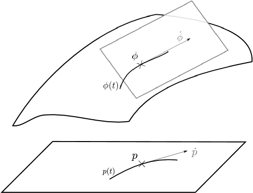
Figure 3. Heuristic visualization of the tangent space to the solution manifold.

2.6. Modelling the Malliavin derivative $\delta\Pi$ by ${\rm d}\Gamma_{x}^{*}$

We note that (177) and (178) combine to

$$L\delta\Pi=(3\mathsf{z}_{3}\Pi^{2}+c)\delta\Pi+\delta\xi\mathsf{1}\quad\mbox{ mod analytic functions};$$

since $\delta\xi$ is not analytic, we cannot simply apply the insight of the previous Subsection 2.5 to $\dot{\Pi}=\delta\Pi$. However, since $\delta\xi\in\dot{H}^{s}$ has some regularity, we expect that the left statement in (2.5) holds approximately. More precisely, since $L$ is of second order and in view of (81), we expect that there exist random $\{{\rm d}\pi_{x}^{({\bf n})}\}_{|{\bf n}|<2+s}$ $\subset\mathbb{R}[[\mathsf{z}_{3},\mathsf{z}_{\bf n}]]$ such that

(187) $$\delta\Pi-\sum_{|{\bf n}|<2+s}{\rm d}\pi_{x}^{({\bf n})}\Gamma_{x}^{*}\partial_{\mathsf{z}_{\bf n}}\Pi_{x}=O(|\cdot-x|^{2+s}).$$

Note that by definition (64), $2+s$ $=\alpha+\frac{D}{2}$, so that in view of (86) and (165) we always have that $2+s>0$. Property (187) motivates to introduce the random endomorphism of $\mathbb{R}[[\mathsf{z}_{3},\mathsf{z}_{\bf n}]]$ via

(188) $${\rm d}\Gamma_{x}^{*}:=\sum_{|{\bf n}|<2+s}{\rm d}\pi_{x}^{({\bf n})}\Gamma_{x}^{*}\partial_{\mathsf{z}_{\bf n}}.$$

We observe in passing that ${\rm d}\Gamma_{x}^{*}$ has the finiteness property (128), as a sum of products of operators that have this property; the latter was already established for $\Gamma_{x}^{*}$ and $\partial_{\mathsf{z}_{\bf n}}$, and is obvious for the operator $M$ of multiplication with an $\pi\in\mathbb{R}[[\mathsf{z}_{3},\mathsf{z}_{\bf n}]]$, which has the coordinate representation $M^{\gamma}_{\beta}$ $=\pi_{\beta-\gamma}$ with the understanding that this matrix element vanishes unless $\gamma\leq\beta$ (coordinate-wise).

We shall indeed establish a Schwartz-distributional version of (187), see (218) below, namely

(189) $$(\delta\Pi-{\rm d}\Gamma_{x}^{*}\Pi_{x})_{r}(x)=O(r^{2+s})\quad\mbox{as}\;r\downarrow 0\;\mbox{for all}\;x\in\mathbb{R}^{1+d}.$$

In this sense, $\delta\Pi_{\beta}$ is described (“modelled” in the jargon of regularity structures) in terms of $\{\Pi_{x\gamma}\}$ to order $2+s$; the coefficients are given by $\{({\rm d}\Gamma_{x}^{*})_{\beta}^{\gamma}\}$ (they combine to a “modelled distribution” $\{({\rm d}\Gamma_{x}^{*})_{\beta}^{\gamma}\}_{\gamma,x}$). The statement (189) is a multi-dimensional version of Gubinelli’s controlled rough-path condition. We note that by the (qualitative) smoothness of $\delta\Pi$ and $\Pi_{x}$ for $\rho>0$, (189) implies

(190) $$\partial^{\bf n}(\delta\Pi-{\rm d}\Gamma_{x}^{*}\Pi_{x})(x)=0\quad\mbox{for}\;|{\bf n}|<2+s,$$

and shall argue in the next Subsection 2.7 that this determines ${\rm d}\Gamma_{x}^{*}$.

2.7. Uniqueness of ${\rm d}\Gamma_{x}^{*}$

By definition (188), we see that (119) and (182) translate into

(191) $${\rm d}\Gamma^{*}_{x}\pi\pi^{\prime}=({\rm d}\Gamma^{*}_{x}\pi)(\Gamma^{*}_{x}\pi^{\prime})+(\Gamma^{*}_{x}\pi)({\rm d}\Gamma^{*}_{x}\pi^{\prime})\quad\mbox{and}\quad{\rm d}\Gamma^{*}_{x}\mathsf{1}=0,$$

(192) $${\rm d}\Gamma^{*}_{x}\mathsf{z}_{3}=0.$$

For later purpose, we note that (192) yields the counterpart of (122)

(193) $${\rm d}\Gamma_{x}^{*}c=0.$$

The three above properties motivate our notation of ${\rm d}$: ${\rm d}\Gamma_{x}^{*}$ like the Malliavin derivative $\delta\Gamma_{x}^{*}$ (which will not play a role in these notes) can be considered as a tangent vector to the group of automorphisms of the algebra $\mathbb{R}[[\mathsf{z}_{3},\mathsf{z}_{\bf n}]]$ in the group element $\Gamma_{x}^{*}$.

However, ${\rm d}\Gamma_{x}^{*}$ does not have the population properties of a tangent vector to the structure group in $\Gamma_{x}^{*}$ (like $\delta\Gamma_{x}^{*}$ is): We immediately obtain from (188) the population condition

(194) $${\rm d}\Gamma^{*}_{x}\mathsf{z}_{\bf n}=0\quad\mbox{unless}\;|{\bf n}|<2+s.$$

As a consequence of (191) & (192) in conjunction with (194), and due to its finiteness property, ${\rm d}\Gamma^{*}_{x}$ is determined by its values on the finitely many coordinates $\{\mathsf{z}_{\bf n}\}_{|{\bf n}|<2+s}$.

We now use these algebraic properties to argue, mimicking the uniqueness argument for $\Gamma^{*}_{x}$ of Subsection 1.19, that via (190),

(195) $${\rm d}\Gamma_{x}^{*}\quad\mbox{is determined by}\;\delta\Pi,\;\mbox{next to}\;\Pi_{x},\Gamma_{x}^{*}.$$

Proof of (195).

Indeed, by (190),

(196) $${\rm d}\Gamma_{x}^{*}\partial^{\bf n}\Pi_{x}(x)\quad\mbox{is determined for $|{\bf n}|<2+s$}.$$

We now argue by induction in $k=|{\bf n}|<2+s$ that ${\rm d}\Gamma_{x}^{*}\mathsf{z}_{\bf n}$ is determined, which by the above determines ${\rm d}\Gamma_{x}^{*}$. The base case $k=0$, which just contains ${\bf n}={\bf 0}$, follows from (196), appealing to (139) and (192). For the induction step $k-1\leadsto k$ we give ourselves an ${\bf n}$ with $|{\bf n}|=k$. By induction hypothesis and (191) & (192), we already identified ${\rm d}\Gamma_{x}^{*}$ on $\mathbb{R}[[\mathsf{z}_{3},\{\mathsf{z}_{\bf m}\}_{|{\bf m}|<k}]]$. Hence via (139) we learn from this and (196) that ${\rm d}\Gamma_{x}^{*}\mathsf{z}_{\bf n}$ is determined. ∎

2.8. A robust relation $\delta\Pi\mapsto\delta\Pi^{-}$

We now claim that (190) implies

(197) $$(\delta\Pi^{-}-\delta\xi_{\rho}\mathsf{1}-{\rm d}\Gamma_{x}^{*}\Pi_{x}^{-})(x)=0.$$

The combination of (190) and (197) provides the desired robust map $\delta\Pi\mapsto\delta\Pi^{-}$ that substitutes the non-robust $\Pi\mapsto\Pi^{-}$ given by (36); in the sense that it bypasses the divergent $c$: In view of (195), ${\rm d}\Gamma_{x}^{*}$ is uniquely determined by (189) in terms of $\delta\Pi$ (at given $\Pi_{x},\Gamma_{x}^{*}$), so that (197) determines $\delta\Pi^{-}$ (at given $\Pi_{x},\Pi_{x}^{-},\Gamma_{x}^{*}$ and of course $\delta\xi$). Hence the mission of Subsection 2.4 is accomplished.

Proof of (197).

We start the argument for (197) by noting that (190) implies in particular

$$(\delta\Pi-{\rm d}\Gamma_{x}^{*}\Pi_{x})(x)=0.$$

In view of (110) and (177), we may pass from this to (197) based on the identity

$${\rm d}\Gamma_{x}^{*}(\mathsf{z}_{3}\Pi_{x}^{3}+c\Pi_{x}+\xi_{\rho}\mathsf{1})=(3\mathsf{z}_{3}\Pi^{2}+c){\rm d}\Gamma_{x}^{*}\Pi_{x},$$

which itself follows from the rules (191) & (192) & (193), the rules (119) & (120) they are based on, and (121). ∎

2.9. Population of ${\rm d}\Gamma_{x}^{*}$

We claim that in analogy to (142) & (143) we have the population property

(198) $$\mbox{for all populated $\gamma$}:\quad({\rm d}\Gamma_{x}^{*})_{\beta}^{\gamma}=0\quad\mbox{unless}\;[\beta]\geq 0.$$

For $\beta=0$, we claim the more precise information

(199) $$({\rm d}\Gamma_{x}^{*})_{0}^{\gamma}=0\quad\mbox{unless}\;\gamma=\delta_{\bf n}\;\mbox{with}\;|{\bf n}|<2+s.$$

Proof of (198) & (199).

We follow Subsection 1.20 and establish (198) by induction in $|\beta|$. We follow the argument for (142) & (143), just indicating the changes. By the last item in (191), the case of $\gamma=0$ is automatically satisfied. As in Subsection 1.20, we start with the cases (146) & (147). Since the Ansatz (145) translates into $\mathsf{z}^{\gamma}$ $=\mathsf{z}_{3}^{k}\prod_{j=1}^{l}\mathsf{z}_{{\bf n}_{j}}$, we learn from (119) & (120) and from (191) & (192) that ${\rm d}\Gamma_{x}^{*}\mathsf{z}^{\gamma}$ is a (finite) linear combination of terms of the form $\mathsf{z}_{3}^{k}$ $({\rm d}\Gamma_{x}^{*}\mathsf{z}_{{\bf n}_{1}})$ $\prod_{j=2}^{l}\Gamma_{x}^{*}\mathsf{z}_{{\bf n}_{j}}$. Hence in view of (127) we obtain the analogue of (149):

$$({\rm d}\Gamma_{x}^{*})^{\gamma}_{\beta}=\mbox{linear combination of}\quad({\rm d}\Gamma_{x}^{*})^{\delta_{{\bf n}_{1}}}_{\beta_{1}}(\Gamma_{x}^{*})^{\delta_{{\bf n}_{2}}}_{\beta_{2}}\cdots(\Gamma_{x}^{*})^{\delta_{{\bf n}_{l}}}_{\beta_{l}}$$

(200) $$\mbox{where}\;k\delta_{3}+\beta_{1}+\cdots+\beta_{l}=\beta.$$

As in Subsection 1.20 we argue that $|\beta_{j}|<|\beta|$ for $j=1,\dots,l$. On the one hand, for $j=1$ we learn from the induction hypothesis that the r. h. s. term in (2.9) vanishes unless $[\beta_{1}]\geq 0$. For $j=2,\dots,l$ we infer from (141) that it vanishes unless $\beta_{j}$ is populated and thus in particular $[\beta_{j}]\geq-1$. Hence by additivity of $[\cdot]$ we learn that $[\beta]{\geq 2k-l+1}$. On the other hand, by (145) we have $[\gamma]$ $=2k-l$, and since $\gamma$ is assumed to be populated so that $[\gamma]+1\geq 0$ we have $2k-l+1\geq 0$. In combination, we obtain the desired $[\beta]\geq 0$.

We conclude the induction step for (198) by treating the case of (148), i. e.  $\gamma=\delta_{\bf n}$. According to (194) we may restrict to the case ${|{\bf n}|<2+s}$. We rewrite (190) component-wise $\partial^{\bf n}\delta\Pi_{\beta}(x)=\sum_{\gamma}({\rm d}\Gamma_{x}^{*})_{\beta}^{\gamma}\partial^{\bf n}\Pi_{x\gamma}(x)$. Splitting the sum into $\gamma$ that are pp, on which we use (109), and those that are not, we obtain the representation

$$({\rm d}\Gamma_{x}^{*})_{\beta}^{\delta_{\bf n}}=\tfrac{1}{{\bf n}!}\partial^{\bf n}\delta\Pi_{\beta}(x)-\sum_{\gamma\textnormal{ not pp}}({\rm d}\Gamma_{x}^{*})_{\beta}^{\gamma}\tfrac{1}{{\bf n}!}\partial^{\bf n}\Pi_{x\gamma}(x).$$

In view of (43), the second factor $\partial^{\bf n}\Pi_{x\gamma}(x)$ vanishes unless $\gamma$ is populated; if $\gamma$ is populated, in view of what we showed in the previous paragraph, the first factor $({\rm d}\Gamma_{x}^{*})_{\beta}^{\gamma}$ vanishes unless $[\beta]\geq 0$. In view of again (43) and its Malliavin derivative, the first term $\partial^{\bf n}\delta\Pi_{\beta}(x)$ vanishes unless $[\beta]\geq 0$. This concludes the induction step and thus the induction argument for (198).

We finally tackle (199). Writing $\gamma$ as in (145), we obtain (2.9) with $\beta_{j}=0$ for all $j=1,\dots,l$; it vanishes unless $k=0$. Since by (73) and (86) we have $|\delta_{{\bf n}_{j}}|$ $=|{\bf n}_{j}|$ $\geq 0$ $>|0|$, it follows from (152) that $(\Gamma_{x}^{*})_{0}^{\delta_{{\bf n}_{j}}}$ $=0$, so that (2.9) vanishes unless $l=1$. Thus $\gamma$ is pp, i. e. $\gamma$ $=\delta_{\bf n}$; the remainder of (199) thus follows from (194). ∎

2.10. Strict triangularity of ${\rm d}\Gamma_{x}^{*}$, order $\prec$ of induction

Theorem 1 is established inductively in $\beta$; in view of (43), (50), (132), (142), and (144) it is sufficient to treat $\beta$ with $[\beta]\geq 0$. The inductive proof relies on triangular properties, in particular those of ${\rm d}\Gamma_{x}^{*}$. While ${\rm d}\Gamma_{x}^{*}$ has the same algebraic properties as $\delta\Gamma_{x}^{*}$, namely (191) & (192), its population pattern is quite different, cf. (194). As a consequence, ${\rm d}\Gamma_{x}^{*}$ is not strictly triangular w. r. t. $|\cdot|$; in fact we just have

(201) $$({\rm d}\Gamma_{x}^{*})_{\beta}^{\gamma}=0\quad\mbox{unless}\;|\gamma|<|\beta|+\frac{D}{2},$$

as we shall argue now by induction in $|\beta|$:

Proof of (201).

The base case follows from (199), where we use (1.11), which implies $|0|$ $=s-\frac{D}{2}+2$, and (73). For the induction step we distinguish two cases. If $\gamma$ is of the form (148), i. e. $\gamma=\delta_{\bf n}$, then we conclude by (194) which yields $({\rm d}\Gamma^{*}_{x})_{\beta}^{\gamma}=0$ unless

$$|\gamma|=|\delta_{\bf n}|\stackrel{{\scriptstyle\eqref{temp04}}}{{=}}|{\bf n}|\stackrel{{\scriptstyle\eqref{cw59}}}{{<}}2+s\stackrel{{\scriptstyle\eqref{ap40}}}{{=}}\alpha+\frac{D}{2}\stackrel{{\scriptstyle\eqref{temp08}}}{{\leq}}|\beta|+\frac{D}{2}.$$

If $\gamma$ is of the form (146) or (147), we appeal to (2.9); by (87) we have $|\beta|-|0|$ $=(|k\delta_{3}|-|0|)$ $+\sum_{j=1}^{l}(|\beta_{j}|-|0|)$, by the induction hypothesis and (152), the term only contributes if $|\beta|-|0|$ $>(|k\delta_{3}|-|0|)$ $+\sum_{j=1}^{l}(|\delta_{{\bf n}_{j}}|-|0|)$ $-\frac{D}{2}$, which by (145) and once more by (87) amounts to the desired $|\beta|-|0|$ $>(|\gamma|-|0|)$ $-\frac{D}{2}$. ∎

For the proof of Theorem 1, we need to find an order $\prec$ on the multi-indices $\beta$ with $[\beta]\geq 0$ w. r. t. which both $\Gamma_{x}^{*}$ and ${\rm d}\Gamma_{x}^{*}$ are strictly triangular. Here are the three properties of the ordinal $|\beta|_{\prec}$ we need: On the subset of multi-indices the induction takes place, the basic feature (87) is required:

$$\mbox{for $\beta$ with $[\beta]\geq 0$}:$$

(202) $$|\cdot|_{\prec}-|0|_{\prec}\;\mbox{is additive},\quad\geq 0,\quad\mbox{and $=0$ only for $\beta=0$}.$$

The ordinal needs to be comparable to $|\cdot|$ in the sense of

(203) $$\mbox{for populated $\beta$}:\quad|\beta|_{\prec}\geq|\beta|\quad\mbox{and}\quad|\delta_{\bf n}|_{\prec}=|\delta_{\bf n}|$$

(which also ensures that coercivity, cf. (88), is preserved), and the ordinal needs to dominate the truncation order of ${\rm d}\Gamma_{x}^{*}$, see (194):

(204) $$\mbox{for $\beta$ with $[\beta]\geq 0$}:\quad|\beta|_{\prec}\geq 2+s.$$

Since $[\beta]+1\geq 0$ for populated $\beta$ and $[\beta]+1=0$ for purely polynomial $\beta$, cf. (55), it follows from (86) and (87) in conjunction with $2+s$ $=\alpha+\frac{D}{2}$, cf. (64), that these postulates are satisfied by

(205) $$|\beta|_{\prec}:=|\beta|+\frac{D}{2}([\beta]+1).$$

We note that $|\beta|_{\prec}$ differs from $|\beta|$, in its representation (1.11), by replacing the pre-factor $s-\frac{D}{2}$ of the noise homogeneity $[\beta]+1$ by $s$.

We claim the strict triangularities

(206) $$\mbox{for all $\gamma$}: \quad(\Gamma_{x}^{*}-{\rm id})_{\beta}^{\gamma}=0\quad\mbox{unless}\;|\gamma|_{\prec}<|\beta|_{\prec},$$

(207) $$\mbox{for all $\gamma$}: \quad({\rm d}\Gamma_{x}^{*})_{\beta}^{\gamma}=0\quad\mbox{unless}\;|\gamma|_{\prec}<|\beta|_{\prec}.$$

Proof of (206) & (207).

The strict triangularity (206) is established closely following the argument for (152) in Subsection 1.21, which is based on induction in $|\beta|$. We start with the base case of $\beta=0$; by (87), (152) assumes the form that $(\Gamma_{x}^{*}-{\rm id})_{0}^{\gamma}=0$ for all $\gamma$, which trivially implies (206). In the induction step, we distinguish whether $\gamma$ is purely polynomial or not, following (156). In case of $\gamma\not=$ pp, we may reproduce the argument for (152) with $|\cdot|$ replaced by $|\cdot|_{\prec}$ since the inspection of it reveals that it only relies on (2.10). We now turn to the case of $\gamma=\delta_{\bf n}$; by (142) we may assume that $\beta$ is populated. Hence our requirement (203) ensures that we may pass from (152) to (206). This concludes the proof of (206).

We now turn to (207) which we establish by induction in the plain length $\gamma(3)+\sum_{\bf n}\gamma({\bf n})$. For $\gamma=0$ and $\gamma=\delta_{3}$ we have $({\rm d}\Gamma^{*}_{x})_{\beta}^{\gamma}=0$ by the second item in (191) and by (192), respectively. For $\gamma=\delta_{\bf n}$ we note that by (194) we have on the one hand $({\rm d}\Gamma_{x}^{*}\mathsf{z}_{\bf n})_{\beta}=0$ unless $|{\bf n}|<2+s$, which by (73), the second item in (127), and (203), translates into $({\rm d}\Gamma_{x}^{*})_{\beta}^{\delta_{\bf n}}=0$ unless $|\delta_{\bf n}|_{\prec}<2+s$. On the other hand, since the purely polynomial $\gamma=\delta_{\bf n}$ is in particular populated, we may by (198) restrict to $[\beta]\geq 0$, so that by postulate (204) we have $|\beta|_{\prec}\geq 2+s$. Both statements combine into the desired statement $({\rm d}\Gamma_{x}^{*})_{\beta}^{\delta_{\bf n}}=0$ unless $|\delta_{\bf n}|_{\prec}<|\beta|_{\prec}$.

Turning to the induction step we are given a $\gamma$ of plain length $\geq 2$, which we write as $\gamma=\gamma_{1}+\gamma_{2}$ with $\gamma_{1}$ and $\gamma_{2}$ of plain length strictly less than that of $\gamma$. As for (2.9), this implies

(208) $$({\rm d}\Gamma^{*}_{x})_{\beta}^{\gamma}=\sum_{\beta_{1}+\beta_{2}=\beta}\big{(}({\rm d}\Gamma^{*}_{x})_{\beta_{1}}^{\gamma_{1}}(\Gamma^{*}_{x})_{\beta_{2}}^{\gamma_{2}}+(\Gamma^{*}_{x})_{\beta_{1}}^{\gamma_{1}}({\rm d}\Gamma^{*}_{x})_{\beta_{2}}^{\gamma_{2}}\big{)}.$$

According to additivity of $|\cdot|_{\prec}-|0|_{\prec}$, $|\gamma|_{\prec}\geq|\beta|_{\prec}$ would imply $|\gamma_{1}|_{\prec}$ $+|\gamma_{2}|_{\prec}$ $\geq|\beta_{1}|_{\prec}$ $+|\beta_{2}|_{\prec}$, and thus $|\gamma_{1}|_{\prec}\geq|\beta_{1}|_{\prec}$ or $|\gamma_{2}|_{\prec}\geq|\beta_{2}|_{\prec}$; w. l. o. g. we may restrict to the former. In this case the first term in (208) vanishes because its first factor vanishes by induction hypothesis. By (206), the second term vanishes unless $\gamma_{1}=\beta_{1}$ which implies $\gamma_{2}=\beta_{2}$, so that also this term vanishes by induction hypothesis. ∎

2.11. Usage of the spectral gap inequality

It is well-known, see [Bog98, Theorem 5.5.1], that for a (centered) Gaussian ensemble that satisfies (164), the variance of a random variable $F$ is dominated by the expectation of the carré-du-champs of its Malliavin derivative

(209) $$\Big{\|}\frac{\partial F}{\partial\xi}\Big{\|}_{\dot{H}^{-s}}^{2}=\Big{(}\sup_{\delta\xi}\frac{\delta F}{\|\delta\xi\|_{\dot{H}^{s}}}\Big{)}^{2}$$

in the sense of

(210) $$\mathbb{E}(F-\mathbb{E}F)^{2}\leq\mathbb{E}\Big{\|}\frac{\partial F}{\partial\xi}\Big{\|}_{\dot{H}^{-s}}^{2}$$

for any (reasonable) random variable $F$ – we continue to be informal. Note that (164) is a special case of (210) for the simple cylinder function(al) $F[\xi]=(\xi,\zeta)$. The inequality (210) can be seen as a Poincaré inequality in probability; it bounds the spectral gap of the generator of the stochastic process that is defined on the basis of the Dirichlet form on the r. h. s of (210) and has the ensemble at hand as a stationary measure. Our assumption of Gaussianity in conjunction with (164) can be replaced by directly assuming (210) (and the closability of the Malliavin derivative).

An easy argument based on Leibniz’ rule and Hölder’s inequality (see e.g. [IORT23, Proposition 5.1]) shows that (210) can be upgraded to the following $\mathbb{E}^{\frac{1}{p}}|\cdot|^{p}$-version for any $2\leq p<\infty$

(211) $$\mathbb{E}^{\frac{1}{p}}|F-\mathbb{E}F|^{p}\lesssim\mathbb{E}^{\frac{1}{p}}\Big{\|}\frac{\partial F}{\partial\xi}\Big{\|}_{\dot{H}^{-s}}^{p},$$

where the implicit constant depends on $p$. In view of (209), (211) can be reformulated as

$$\mathbb{E}^{\frac{1}{p}}|F-\mathbb{E}F|^{p} \lesssim\sup_{\delta\xi\;\textnormal{random}}\frac{\mathbb{E}\delta F}{\mathbb{E}^{\frac{1}{p^{*}}}\|\delta\xi\|_{\dot{H}^{s}}^{p^{*}}}$$

$$=\sup\{\,\mathbb{E}\delta F\,|\,\delta\xi\;\mbox{random with}\;\mathbb{E}\|\delta\xi\|_{\dot{H}^{s}}^{p^{*}}\leq 1\,\},$$

where $1<p^{*}\leq 2$ is the dual exponent to $p$, i. e. $\frac{1}{p}+\frac{1}{p^{*}}=1$. Hence our task at hand is to estimate $\delta F$ for random variables of interest like $F=\Pi_{\beta r}^{-}(0)$. In fact, for the induction argument, it will be important to monitor a norm instead of its expectation, namely

(212) $$\mathbb{E}^{\frac{1}{q}}|\delta\Pi_{\beta r}^{-}(0)|^{q}\quad\mbox{for all}\;1\leq q<p^{*}\leq 2\leq p.$$

That is, we will use the spectral gap assumption in the form

$$\mathbb{E}^{\frac{1}{p}}|\Pi_{\beta r}^{-}(0)|^{p} \lesssim|\mathbb{E}\Pi_{\beta r}^{-}(0)|$$

(213) $$\quad+\sup\{\,\mathbb{E}^{\frac{1}{q}}|\delta\Pi_{\beta r}^{-}(0)|^{q}\,|\,\delta\xi\;\mbox{random with}\;\mathbb{E}\|\delta\xi\|_{\dot{H}^{s}}^{p^{*}}\leq 1\,\}.$$

In what follows, all estimates will be proved simultaneously for all $p,q$ in the range (212) (with implicit constants depending on $p,p^{*},q$), so that it will not be a problem to recursively appeal to the same estimates with exponents $q^{\prime}\in(q,p^{*})$ or $p^{\prime}>p$, as happens e.g. when applying Hölder’s inequality in probability. In practice: Within the induction we fix $p,q$ and a random $\delta\xi\in\dot{H}^{s}$ with

(214) $$\mathbb{E}\|\delta\xi\|_{\dot{H}^{s}}^{p^{*}}\leq 1,$$

and estimate Malliavin derivatives in the direction $\delta\xi$.

In order to complete the argument (213), also the expectation $|\mathbb{E}\Pi_{\beta r}^{-}(0)|$ has to be bounded. This will follow from (92), see Subsection 3.4. This relies on the BPHZ-choice of renormalization, so that this requires the restriction to $|\beta|<2$.

2.12. Besov-type norms and base case

At the core of the proof is a quantification of (189). From now onwards, we restrict ourself to $\beta$ with $[\beta]\geq 0$ and $|\beta|<2$ (the case $|\beta|>2$ is treated differently, see Subsection 2.17). We start by noting

$$L(\delta\Pi-{\rm d}\Gamma_{x}^{*}\Pi_{x})_{\beta}-(\delta\Pi^{-}-{\rm d}\Gamma_{x}^{*}\Pi_{x}^{-})_{\beta}$$

(215) $$=0\quad\mbox{ mod polynomials of degree $<|\beta|+\frac{D}{2}-2$}.$$

Indeed, this follows from (111), (178), and (201).

We momentarily consider the base case $\beta=0$; in view of (1.11), the polynomial in (2.12) is of degree $<s$, and according to (30) and (199), (2.12) thus collapses to

$$L\big{(}\delta\Pi_{0}-\sum_{|{\bf n}|<2+s}({\rm d}\Gamma_{x}^{*})_{0}^{\delta_{\bf n}}(\cdot-x)^{\bf n}\big{)}=\delta\xi\mbox{ mod polynomials of degree}<s.$$

This shows that the order of truncation of what now is a Taylor polynomial of order $<2+s$ of $\delta\Pi_{0}$ is consistent with the order of regularity $s$ of $\delta\xi$ and the order $2$ of $L$. It also shows that in its pointwise-in-$x$ form, statement (189) is too strong; in fact, because of the $L^{2}$-based nature of $\dot{H}^{s}$ we only have

$$\big{(}\int dx|\delta\Pi_{0}(x+y)-\sum_{|{\bf n}|<2+s}({\rm d}\Gamma_{x}^{*})_{0}^{\delta_{\bf n}}y^{\bf n}|^{2}\big{)}^{\frac{1}{2}} \lesssim|y|^{2+s}\|\delta\Pi_{0}\|_{\dot{H}^{2+s}}$$

$$\lesssim|y|^{2+s}\|\delta\xi\|_{\dot{H}^{s}},$$

which is easily seen by Fourier transformation. This amounts to an estimate of $\delta\Pi_{0}$ in the Besov space $\dot{B}^{2+s}_{2,\infty}$. Because of Minkowski’s inequality (recall $q\leq 2$) and the normalization (214), it implies the “annealed” estimate

(216) $$\big{(}\int dx\mathbb{E}^{\frac{2}{q}}|\delta\Pi_{0}(x+y)-\sum_{|{\bf n}|<2+s}({\rm d}\Gamma_{x}^{*})_{0}^{\delta_{\bf n}}y^{\bf n}|^{q}\big{)}^{\frac{1}{2}}\lesssim|y|^{2+s}.$$

What can we expect for $(\delta\Pi-{\rm d}\Gamma_{x}^{*}\Pi_{x})_{\beta}$ with $\beta\not=0$? First of all, as discussed in Subsection 2.4 in case of $\beta=\delta_{3}$, we cannot expect to estimate $\delta\Pi_{\beta}$ as a (square-integrable) function, but just as a distribution. Hence in anticipation, we relax (216) to

(217) $$\big{(}\int dx\mathbb{E}^{\frac{2}{q}}|\big{(}\delta\Pi-{\rm d}\Gamma_{x}^{*}\Pi_{x})_{0r}(x)|^{q}\big{)}^{\frac{1}{2}}\lesssim r^{2+s}\stackrel{{\scriptstyle\eqref{ap40}}}{{=}}r^{\alpha+\frac{D}{2}},$$

where the constant now implicitly depends on the control (2). Moreover, in view of its structure (2.9), ${\rm d}\Gamma_{x}^{*}$ will acquire (some of) the growth (159) of $\Gamma_{x}^{*}$ in $x$, while according to (113), the law of $\Pi_{x\gamma r}(x)$ is independent of $x$, so that one cannot expect $\mathbb{E}^{\frac{1}{q}}|({\rm d}\Gamma_{x}^{*}\Pi_{x})_{\beta r}(x)|^{q}$ to be square integrable (at infinity) in $x$. Hence for $\beta\not=0$, we need to relax (217) by restricting the $x$-integral to a (parabolic) ball ${B_{R}:=\{|x|<R\}}$. So next to the mollification length scale $r$, we acquire a second length scale, the localization scale $R$. This motivates the form of the l. h. s. of

(218) $$\big{(}\int_{B_{R}}dx\mathbb{E}^{\frac{2}{q}} |(\delta\Pi-{\rm d}\Gamma_{x}^{*}\Pi_{x})_{\beta r}(x)|^{q}\big{)}^{\frac{1}{2}}\lesssim r^{\alpha+\frac{D}{2}}(r+R)^{|\beta|-\alpha},$$

which is indeed what we shall establish – and just have established for $\beta=0$ in view of (86).

Note that compared to (169), passing from $\Pi$ to $\delta\Pi-{\rm d}\Gamma_{x}^{*}\Pi_{x}$ comes with a (beneficial) factor of $r^{\frac{D}{2}}$, and $R$ plays the role of $|x|$. There are two consistency checks for the two exponents in (218): 1) For $r\ll R$, (218) contains the expected $O(r^{\alpha+\frac{D}{2}=2+s})$-behavior of (189). 2) The dimension in terms of length of (218) is consistent with the one of (169) since the $L^{2}(B_{R})$-norm contributes $\frac{D}{2}$ dimensions of length.

While we have established (218) in the base case of $\beta=0$, for $\beta\not=0$, we shall derive it by “integration” of (2.12) from

(219) $$\big{(}\int_{B_{R}}dx\mathbb{E}^{\frac{2}{q}}|(\delta\Pi^{-}-{\rm d}\Gamma_{x}^{*}\Pi_{x}^{-})_{\beta r}(x)|^{q}\big{)}^{\frac{1}{2}}\lesssim r^{\alpha-2+\frac{D}{2}}(r+R)^{|\beta|-\alpha}.$$

In fact we shall establish the slightly stronger

(220) $$\big{(}\int_{B_{R}}dx\mathbb{E}^{\frac{2}{q}}|(\delta\Pi^{-}-{\rm d}\Gamma_{x}^{*}\Pi_{x}^{-})_{\beta r}(x)|^{q}\big{)}^{\frac{1}{2}}\lesssim r^{3\alpha+\frac{D}{2}}(r+R)^{|\beta|-2-3\alpha},$$

which, as a quantitative version of (197) (recall $3\alpha+\frac{D}{2}>0$ by assumption (165)), is the estimate required for the characterization of the model in [Tem23]. The next four subsections are devoted to the induction step that establishes (218) & (220). It will be based on the four consecutive steps of an algebraic argument, reconstruction, integration, and a three-point argument; in this section, we shall focus on the algebraic aspects of all steps, while the analytic ingredients will be detailed in Section 3. As it turns out, these arguments do not use the fact that $\delta\Pi$ and $\delta\Pi^{-}$ are Malliavin derivatives in direction of $\delta\xi$, but just rely on the relations (177) & (178), and the control (214). Hence we actually provide an a priori estimate for the inverse of the linearization of $\dot{\phi}\mapsto L\dot{\phi}-(3\lambda\phi^{2}+h^{({\rho})})\dot{\phi}$, on our term-by-term level, and in an $L^{2}$-based norm. Hence our approach blends solution theory and stochastic estimates.

The induction step laid out in the next four subsections is restricted to multi-indices $\beta$ with $|\beta|<$ $\lceil s+2\rceil$, which is needed for integration. Hence in our induction w. r. t. $|\cdot|_{\prec}$, we have to ensure that we only use the induction hypothesis under this additional constraint. The range $|\beta|<$ $\lceil s+2\rceil$ does cover the desired range of $|\beta|<2$ iff $1<s+2=\alpha+\frac{D}{2}$, which in view of (165) and $\alpha<0$ is the case iff $D\geq 3$, which we have assumed.

2.13. The algebraic argument for ${\rm d}\Gamma_{x+y}^{*}-{\rm d}\Gamma_{x}^{*}\Gamma_{x\,x+y}^{*}$

Estimate (220) will be a consequence of what in regularity structures is called reconstruction. It states that a distribution like $\delta\Pi_{\beta}$ can be “reconstructed” from the family of distributions like $\{({\rm d}\Gamma_{x}^{*}\Pi_{x}^{-})_{\beta}\}_{x}$ that act as germs near every space-time point $x$. For this to be canonically feasible, the distributions $({\rm d}\Gamma_{x}^{*}\Pi_{x}^{-})_{\beta}$ have to satisfy a continuity condition w. r. t. the base-point $x$, see (2.14) below. In the next Subsection 2.14, (2.14) is derived from graded continuity of $\{({\rm d}\Gamma_{x}^{*}\Gamma_{x}^{-*})_{\beta}^{\gamma}\}_{\gamma}$ in $x$. In line with the continuity condition on modelled distributions in regularity structures, this graded continuity is formulated in terms of smallness of the increment ${\rm d}\Gamma^{*}_{x+y}-{\rm d}\Gamma_{x}^{*}\Gamma_{x\;x+y}^{*}$ in terms of the shift $y$, where by (153) $\Gamma_{x\;x+y}^{*}=\Gamma_{x}^{-*}\Gamma_{x+y}^{*}$. Also this graded continuity is formulated in an $L^{2}(B_{R})$ sense:

$$\mbox{for populated $\gamma$}:\quad\big{(}\int_{B_{R}}dx\mathbb{E}^{\frac{2}{q}}|({\rm d}\Gamma^{*}_{x+y}-{\rm d}\Gamma_{x}^{*}\Gamma_{x\;x+y}^{*})_{\beta}^{\gamma}|^{q}\big{)}^{\frac{1}{2}}$$

(223) $$\lesssim\left\{\begin{array}[]{clc}|y|^{\alpha-|\gamma|_{p}+\frac{D}{2}}\mbox{}&(|y|+R)^{|\beta|-|\gamma|+|\gamma|_{p}-\alpha}&\mbox{if}\;\alpha-|\gamma|_{p}+\frac{D}{2}>0\\ &(|y|+R)^{|\beta|-|\gamma|+\frac{D}{2}}&\mbox{else}\end{array}\right\},$$

where we have set for abbreviation

(224) $$|\gamma|_{p}:=\sum_{\bf n}|{\bf n}|\gamma({\bf n}),$$

and with the understanding that the

l. h. s. of (2.13) vanishes

(225) $$\mbox{unless}\quad\sum_{\bf n}\gamma({\bf n})\not=0\quad\mbox{and}\quad|\beta|-|\gamma|+|\gamma|_{p}-\alpha\geq 0.$$

Such a “pointed” Besov-type norm (2.13) was introduced in [HS23, Definition 3.9] in a very similar context. This continuity condition (2.13) in $y$ could be strengthened to yield a positive Hölder exponent in all cases; however using (2.13), estimate (2.13) will be sufficient for reconstruction in the full range (165). Note that in fact both alternatives in (2.13) hold, no matter what the sign of $\alpha-|\gamma|_{p}+\frac{D}{2}$ is.

Following (156) in Subsection 1.21, we distinguish the cases of $\gamma$ purely polynomial and $\gamma$ not pp, see Subsection 1.9 for the language. As in Subsection 1.21, we first treat $\gamma$ not pp by a purely algebraic argument in this subsection. We then treat $\gamma$ pp by an analytic argument in Subsection 2.16.

Proof of (2.13) & (2.13) for $\gamma\neq$ pp (algebraic argument).

The argument for (2.13) for $\gamma\not=$ pp relies on the fact that (119) & (120) transmit to $\Gamma_{x\;x+y}^{*}$, and that (191) & (192) transmit to the endomorphism ${S:={\rm d}\Gamma_{x+y}^{*}-{\rm d}\Gamma_{x}^{*}\Gamma_{x\;x+y}^{*}}$. As a consequence, as for (2.9) in Subsection 2.9, we have

(226) $$S^{\gamma}_{\beta}=\mbox{linear combination of}\quad S^{\delta_{{\bf n}_{1}}}_{\beta_{1}}(\Gamma_{0\;x+y}^{*})^{\delta_{{\bf n}_{2}}}_{\beta_{2}}\cdots(\Gamma_{0\;x+y}^{*})^{\delta_{{\bf n}_{l}}}_{\beta_{l}}$$

(227) $$\mbox{where}\;k\delta_{3}+\beta_{1}+\cdots+\beta_{l}=\beta\;\;\mbox{if}\;\;k\delta_{3}+\delta_{{\bf n}_{1}}+\cdots+\delta_{{\bf n}_{l}}=\gamma.$$

We note that by (44) and (87)

(230) $$\begin{array}[]{cc}(|k\delta_{3}|-|0|)+|\beta_{1}|+\sum_{j=2}^{l}(|\beta_{j}|-|0|)&=|\beta|,\\ (2k-l+1)+[\beta_{1}]+\sum_{j=2}^{l}([\beta_{j}]+1)&=[\beta].\end{array}$$

Since $\gamma$ is populated but not purely polynomial we have $k\not=0$. Hence we learn from the first row in (230) and (87) that $|\beta_{1}|<|\beta|$. Since $\gamma$ is populated, we have in particular $0\leq[\gamma]+1=2k-l+1$, cf (44). Since by (141) for $j=2,\dots,l$, the r. h. s. of (226) vanishes unless $\beta_{j}$ is populated, and thus $[\beta_{j}]+1\geq 0$. Thus we learn from the second row in (230) that $[\beta_{1}]\leq[\beta]$. Hence $|\beta_{1}|_{\prec}<|\beta|_{\prec}$ by definition (205). Based on (198) rather than (141), we also learn $|\beta_{j}|_{\prec}<|\beta|_{\prec}$ for $j=2,\dots,l$, so that we may use our induction hypothesis.

From (168) (with $p$ replaced by a suitable exponent $p_{j}>p$) and from (2.13) in its form (2.16) for $\gamma$ pp, both in their induction hypothesis version (with $q$ replaced by some exponent $q^{\prime}>q$), we obtain by Hölder’s inequality in probability (provided $\frac{1}{q^{\prime}}+\sum_{j=2}^{l}\frac{1}{p_{j}}=\frac{1}{q}$) applied to (226) an estimate by

$$\min\{|y|^{\alpha-|{\bf n}_{1}|+\frac{D}{2}}(|y|+R)^{|\beta_{1}|-\alpha},(|y|+R)^{|\beta_{1}|-|{\bf n}_{1}|+\frac{D}{2}}\}$$

(231) $$\times(|y|+R)^{|\beta_{2}|-|{\bf n}_{2}|}\cdots(|y|+R)^{|\beta_{l}|-|{\bf n}_{l}|}.$$

According to (152) we have $|\beta_{j}|\geq|{\bf n}_{j}|\geq 0$ for $j=2,\dots,l$, so that (2.13) is $\leq$

$$\min\{|y|^{\alpha-\sum_{j=1}^{l}|{\bf n}_{j}|+\frac{D}{2}}(|y|+R)^{\sum_{j=1}^{l}|\beta_{j}|-\alpha},(|y|+R)^{\sum_{j=1}^{l}|\beta_{j}|-\sum_{j=1}^{l}|{\bf n}_{j}|+\frac{D}{2}}\},$$

(232) $$\quad\mbox{and furthermore}\quad{\textstyle\sum_{j=1}^{l}}|\beta_{j}|-\alpha\geq 0.$$

By definitions (69) and (224) of $|\cdot|$ and $|\cdot|_{p}$, we read off (227) that

$$\begin{array}[]{cl}|\beta|-\alpha&=\sum_{j=1}^{l}|\beta_{j}|-l\alpha+2k(1+\alpha),\\ |\gamma|-\alpha&=\sum_{j=1}^{l}|{\bf n}_{j}|-l\alpha+2k(1+\alpha),\quad\sum_{j=1}^{l}|{\bf n}_{j}|=|\gamma|_{p}.\end{array}$$

These identities show that the exponents in (2.13) coincide with those on the r. h. s. of (2.13). This also shows that the second item in (2.13) is a consequence of the second item in (2.13). Finally, if $l=\sum_{\bf n}\gamma({\bf n})=0$ then $\gamma=k\delta_{3}$ whence $S_{\beta}^{\gamma}=0$ by (120) and (192), proving the first item in (2.13). ∎

2.14. Reconstruction for $\delta\Pi^{-}-{\rm d}\Gamma_{x}^{*}\Pi_{x}^{-}$

We return to our task of deriving (220), which we shall derive from the continuity condition

$$\big{(}\int_{B_{R}}dx \mathbb{E}^{\frac{2}{q}}|({\rm d}\Gamma_{x+y}^{*}\Pi_{x+y}^{-}-{\rm d}\Gamma_{x}^{*}\Pi_{x}^{-})_{\beta r}(x+y)|^{q}\big{)}^{\frac{1}{2}}$$

(233) $$\lesssim r^{2\alpha}(|y|+r)^{\alpha+\frac{D}{2}}(|y|+r+R)^{|\beta|-2-3\alpha},$$

with the implicit understanding that the last exponent is non-negative unless the l. h. s. vanishes. We provide the reconstruction argument proper that establishes (220) based on the assumption (165) and on (2.14) in Subsection 3.2.

Proof of (2.14) (continuity in the base point).

Recalling (154) we have ${\rm d}\Gamma_{x+y}^{*}\Pi_{x+y}^{-}-{\rm d}\Gamma_{x}^{*}\Pi_{x}^{-}$ $=({\rm d}\Gamma_{x+y}^{*}-{\rm d}\Gamma_{x}^{*}\Gamma_{x\;x+y}^{*})\Pi_{x+y}^{-}$. We consider the $\beta$-component, mollify on scale $r$, and evaluate in $x+y$:

$$({\rm d}\Gamma_{x+y}^{*}\Pi_{x+y}^{-}-{\rm d}\Gamma_{x}^{*}\Pi_{x}^{-})_{\beta r}(x+y)$$

(234) $$=\sum_{\gamma}({\rm d}\Gamma_{x+y}^{*}-{\rm d}\Gamma_{x}^{*}\Gamma_{x\;x+y}^{*})_{\beta}^{\gamma}\Pi_{x+y\gamma r}^{-}(x+y).$$

Because of the strict triangularities (206) & (207), the induction hypothesis (167) is sufficient. According to (50), the sum is effectively restricted to populated $\gamma$’s that are non-purely polynomial so that we may appeal to the part of (2.13) we established in Subsection 2.13. Hence the first r. h. s. factor in (2.14) is estimated by $|y|^{\alpha-|\gamma|_{p}+\frac{D}{2}}(|y|$ $+R)^{|\beta|+|\gamma|_{p}-|\gamma|-\alpha}$ and by $(|y|+R)^{|\beta|-|\gamma|+\frac{D}{2}}$. As in Subsection 2.13, we combine the estimate of both factors by Hölder’s inequality to obtain that the l. h. s. of (2.14) is estimated by terms of the form

(235) $$r^{|\gamma|-2}\min\{|y|^{\alpha-|\gamma|_{p}+\frac{D}{2}}(|y|+R)^{|\beta|+|\gamma|_{p}-|\gamma|-\alpha},(|y|+R)^{|\beta|-|\gamma|+\frac{D}{2}}\}.$$

By the first item in (2.13) we have for the populated and non-pp $\gamma$’s effectively appearing in (2.14) that $\gamma(3)\not=0$ and thus

(236) $$|\gamma|-|\gamma|_{p}\stackrel{{\scriptstyle\eqref{ao07}}}{{=}}(1+\alpha)2\gamma(3)+(-\alpha)(\sum_{\bf n}\gamma({\bf n})-1)\stackrel{{\scriptstyle\eqref{ck28}}}{{\geq}}2(1+\alpha).$$

Hence we have in particular $|\gamma|-2\geq 2\alpha$ so that we obtain in case of $\alpha-|\gamma|_{p}+\frac{D}{2}$ $\geq 0$ that the term in (235) is $\leq$

$$r^{|\gamma|-2}|y|^{\alpha-|\gamma|_{p}+\frac{D}{2}}(|y|+R)^{|\beta|+|\gamma|_{p}-|\gamma|-\alpha}$$

$$\stackrel{{\scriptstyle\hphantom{\eqref{ap46},\eqref{ap79}}}}{{\leq}}r^{2\alpha}(|y|+r)^{-\alpha-|\gamma|_{p}+\frac{D}{2}+|\gamma|-2}(|y|+R)^{|\beta|+|\gamma|_{p}-|\gamma|-\alpha}$$

$$\stackrel{{\scriptstyle\eqref{ap46},\eqref{ap79}}}{{\leq}}r^{2\alpha}(|y|+r)^{\alpha+\frac{D}{2}}(|y|+r+R)^{|\beta|-2-3\alpha},$$

as desired. In the remaining case of $\alpha-|\gamma|_{p}+\frac{D}{2}$ $\leq 0$ we have by (236) that $|\gamma|-2$ $\geq 3\alpha+\frac{D}{2}$, so that by the alternative estimate in (235) and $|\beta|-|\gamma|+\frac{D}{2}\geq 0$ (which is a consequence of (152) and (201)), we obtain that the term is $\leq$

$$r^{|\gamma|-2}(|y|+R)^{|\beta|-|\gamma|+\frac{D}{2}} \leq r^{3\alpha+\frac{D}{2}}(|y|+r+R)^{|\beta|-2-3\alpha},$$

$$\leq r^{2\alpha}(|y|+r)^{\alpha+\frac{D}{2}}(|y|+r+R)^{|\beta|-2-3\alpha},$$

again as desired. ∎

2.15. Integration for $\delta\Pi-{\rm d}\Gamma_{x}^{*}\Pi_{x}$

It is not possible to directly pass from the estimate (219) to the estimate (218) via the PDE (2.12). The reason is more algebraic than analytic, as we shall explain now: (2.12) is not sufficient to even characterize $(\delta\Pi-{\rm d}\Gamma_{x}^{*}\Pi_{x})_{\beta}$ in terms of ${(\delta\Pi^{-}-{\rm d}\Gamma_{x}^{*}\Pi_{x}^{-})_{\beta}}$ – even when taking the vanishing (190) in $x$ into account. The reason is that there is a mismatch between the vanishing order $2+s$ of $\delta\Pi_{\beta}$ $-\sum_{\gamma}({\rm d}\Gamma_{x}^{*})_{\beta}^{\gamma}\Pi_{x\gamma}$, and the growth of the same quantity at infinity: In view of (201), the sum extends over all $\gamma$ with $|\gamma|<|\beta|+\frac{D}{2}$, and thus includes terms that grow almost at order $2+\frac{D}{2}$, which is definitely larger than $2+s$. Hence we need to truncate the sum at order $2+s$. For the same reason, we need to restrict to $|\beta|<\lceil 2+s\rceil$. This means that instead of relying on (2.12) we work with

$$L(\delta\Pi_{\beta}-\sum_{|\gamma|<2+s}({\rm d}\Gamma_{x}^{*})_{\beta}^{\gamma}\Pi_{x\gamma})$$

$$=\delta\Pi_{\beta}^{-}-\sum_{|\gamma|<2+s}({\rm d}\Gamma_{x}^{*})_{\beta}^{\gamma}\Pi_{x\gamma}^{-}\quad\mbox{ mod polynomials of degree}<s.$$

This in turn requires to pre-process the input (219) and to post-process the output (218): We need an independent argument that ensures

(237) $$\big{(}\int_{B_{R}}dx\mathbb{E}^{\frac{2}{q}}|\sum_{|\gamma|\geq 2+s}({\rm d}\Gamma_{x}^{*})_{\beta}^{\gamma}\Pi_{x\gamma r}^{-}(x)|^{q}\big{)}^{\frac{1}{2}} \lesssim r^{\alpha-2+\frac{D}{2}}(r+R)^{|\beta|-\alpha},$$

(238) $$\big{(}\int_{B_{R}}dx\mathbb{E}^{\frac{2}{q}}|\sum_{|\gamma|\geq 2+s}({\rm d}\Gamma_{x}^{*})_{\beta}^{\gamma}\Pi_{x\gamma r}(x)|^{q}\big{)}^{\frac{1}{2}} \lesssim r^{\alpha+\frac{D}{2}}(r+R)^{|\beta|-\alpha}.$$

In this subsection, we claim that (237) & (238) follow once we establish

(239) $$\mbox{for populated $\gamma\not=\mbox{pp}$}:\quad\big{(}\int_{B_{R}}dx\mathbb{E}^{\frac{2}{q}}|({\rm d}\Gamma_{x}^{*})_{\beta}^{\gamma}|^{q}\big{)}^{\frac{1}{2}}\lesssim R^{\frac{D}{2}+|\beta|-|\gamma|};$$

by (201) the exponent is effectively positive. Establishing (239) requires a second round of algebraic argument, integration, and three-point argument, see Subsection 2.18. On the other hand, the integration argument proper will be carried out in Subsection 3.7.

Proof that (239) implies (237) & (238).

We start by noting that the restriction to populated $\gamma$ that are not purely polynomial is sufficient for (237) & (238). In case of (237), this follows from (50); in case of (238), this is a consequence of (194). Next, we note that by the strict triangularity (207), the sum in $\gamma$ is restricted to $|\gamma|_{\prec}<|\beta|_{\prec}$ so that we may appeal to the induction hypothesis in form of (166) & (167). Finally, by (201), the (finite) sum is restricted to $|\gamma|$ $<|\beta|+\frac{D}{2}$, next to $|\gamma|$ $\geq 2+s$ $=\alpha+\frac{D}{2}$. Hence by the triangle inequality and Hölder’s inequality, (237) is as desired estimated by

$$\max_{\alpha+\frac{D}{2}\leq|\gamma|<|\beta|+\frac{D}{2}}R^{\frac{D}{2}+|\beta|-|\gamma|}r^{|\gamma|-2}\leq r^{\alpha-2+\frac{D}{2}}(r+R)^{|\beta|-\alpha}.$$

The argument for (238) is very similar. ∎

2.16. The three-point argument for ${\rm d}\Gamma_{x+y}^{*}-{\rm d}\Gamma_{x}^{*}\Gamma_{x\,x+y}^{*}$

In order to close the induction step, we need to establish (2.13) for purely polynomial $\gamma$, that is

$$\big{(}\int_{B_{R}}dx\mathbb{E}^{\frac{2}{q}} |({\rm d}\Gamma^{*}_{x+y}-{\rm d}\Gamma_{x}^{*}\Gamma_{x\;x+y}^{*})_{\beta}^{\delta_{\bf n}}|^{q}\big{)}^{\frac{1}{2}}$$

(242) $$\lesssim\left\{\begin{array}[]{lc}|y|^{\alpha-|{\bf n}|+\frac{D}{2}}(|y|+R)^{|\beta|-\alpha}&\mbox{for}\;\alpha-|{\bf n}|+\frac{D}{2}>0\\ (|y|+R)^{|\beta|-|{\bf n}|+\frac{D}{2}}&\mbox{else}\end{array}\right\}.$$

Proof of (2.16) (three-point argument).

Let us start with the second part of the estimate, which by (64) amounts to the case of $|{\bf n}|\geq s+2$, so that by (194), the l. h. s.  reduces to $-\sum_{\gamma}({\rm d}\Gamma_{x}^{*})_{\beta}^{\gamma}$ $(\Gamma_{x\;x+y}^{*})_{\gamma}^{\delta_{\bf n}}$. Since by (207), the sum is restricted to $|\gamma|_{\prec}<|\beta|_{\prec}$, we may appeal to the induction hypothesis (168) in conjunction with (155) for the second factor. If $\gamma$ were purely polynomial, i. e. of the form $\gamma=\delta_{\bf m}$, then (152) would in conjunction with (73) imply $|{\bf m}|\geq|{\bf n}|$, so that also $|{\bf m}|\geq s+2$, and that by (194), the first factor would vanish. Hence effectively $\gamma\not=$ pp so that for the first factor, we may appeal to (239). Moreover, by (152) and (201), the finite sum restricts to $|\gamma|\geq|{\bf n}|$ and $|\gamma|<|\beta|+\frac{D}{2}$. In conclusion, we obtain by Hölder’s inequality an estimate of the l. h. s. of (2.16) by

$$\max_{|{\bf n}|\leq|\gamma|<|\beta|+\frac{D}{2}}R^{|\beta|-|\gamma|+\frac{D}{2}}|y|^{|\gamma|-|{\bf n}|}\leq(|y|+R)^{|\beta|-|{\bf n}|+\frac{D}{2}},$$

as desired.

We now turn to the first estimate in (2.16), which we derive from (218): We use (154) to write $({\rm d}\Gamma_{x+y}^{*}-{\rm d}\Gamma_{x}^{*}\Gamma_{x\;x+y}^{*})\Pi_{x+y}$ $=-(\delta\Pi-{\rm d}\Gamma_{x+y}^{*}\Pi_{x+y})$ $+(\delta\Pi-{\rm d}\Gamma_{x}^{*}\Pi_{x})$; we consider the $\beta$ component, spell out the matrix vector product and split into purely polynomial $\gamma$, on which we use (109), and the remainder. We then apply $(\cdot)_{r}(x+y)$; this yields the representation

$$\big{(}\sum_{\bf n}({\rm d}\Gamma_{x+y}^{*}-{\rm d}\Gamma_{x}^{*}\Gamma_{x\;x+y}^{*})_{\beta}^{\delta_{\bf n}}(\cdot)^{\bf n}\big{)}_{r}(0)$$

$$=(\delta\Pi-{\rm d}\Gamma_{x}^{*}\Pi_{x})_{\beta r}(x+y)-(\delta\Pi-{\rm d}\Gamma_{x+y}^{*}\Pi_{x+y})_{\beta r}(x+y)$$

(243) $$-\sum_{\gamma\not=\textnormal{pp}}({\rm d}\Gamma_{x+y}^{*}-{\rm d}\Gamma_{x}^{*}\Gamma_{x\;x+y}^{*})_{\beta}^{\gamma}\Pi_{x+y\gamma r}(x+y).$$

We take the $(\int_{B_{R}}dx\mathbb{E}^{\frac{2}{q}}|\cdot|^{q})^{\frac{1}{2}}$ norm. In order to subsume the first r. h. s. term under (218) we introduce $\psi^{(r)}:=\psi(\cdot+R^{-1}y)$, with $R^{-1}$ being the inverse of the transformation (12), so that $\psi_{r}(\cdot+y)$ $=\psi^{(r)}_{r}$, and note that as long as $|y|\leq r$, the semi norms (2) of $\psi^{(r)}$ are controlled by those of $\psi$. Hence we obtain from (218)

$$\big{(}\int_{B_{R}}dx\mathbb{E}^{\frac{2}{q}}|(\delta\Pi-{\rm d}\Gamma_{x}^{*}\Pi_{x})_{\beta r}(x+y)|^{q}\big{)}^{\frac{1}{2}}$$

$$\lesssim r^{\alpha+\frac{D}{2}}(r+R)^{|\beta|-\alpha}\quad\mbox{provided}\;|y|\leq r.$$

For the second r. h. s. term in (2.16) we use the generic estimate

(244) $$\int_{B_{R}}dxf^{2}(x+y)\leq\int_{B_{R+|y|}}dx^{\prime}f^{2}(x^{\prime})$$

together with (218) to obtain like for the first term

$$\big{(}\int_{B_{R}}dx\mathbb{E}^{\frac{2}{q}}|(\delta\Pi-{\rm d}\Gamma_{x+y}^{*}\Pi_{x+y})_{\beta r}(x+y)|^{q}\big{)}^{\frac{1}{2}}$$

$$\lesssim r^{\alpha+\frac{D}{2}}(r+R)^{|\beta|-\alpha}\quad\mbox{provided}\;|y|\leq r.$$

For the last term in (2.16) we note that at this stage of the induction step we do have access to (2.13) for $\gamma$ not purely polynomial; by (206) & (207), only $|\gamma|_{\prec}<|\beta|_{\prec}$ are involved so that we may appeal to (166) on the level of the induction hypothesis. By the triangle inequality, (113) and Hölder’s inequality we obtain, still for $|y|\leq r$,

$$\big{(}\int_{B_{R}}dx\mathbb{E}^{\frac{2}{q}}|\big{(}\sum_{\bf n}({\rm d}\Gamma_{x+y}^{*}-{\rm d}\Gamma_{x}^{*}\Gamma_{x\;x+y}^{*})_{\beta}^{\delta_{\bf n}}(\cdot)^{\bf n}\big{)}_{r}(0)|^{q}\big{)}^{\frac{1}{2}}$$

$$\lesssim r^{\alpha+\frac{D}{2}}(r+R)^{|\beta|-\alpha}+\sum_{\begin{subarray}{c}\gamma:|\gamma|_{\prec}<|\beta|_{\prec}\\ |\gamma|\geq|\gamma|_{p}\end{subarray}}|y|^{\alpha-|\gamma|_{p}+\frac{D}{2}}(r+R)^{|\beta|-|\gamma|+|\gamma|_{p}-\alpha}r^{|\gamma|},$$

where the restriction to $|\gamma|\geq|\gamma|_{p}$ follows by definitions (69) and (224) from the first item in (2.13). We use this for $r=|y|$, in which it simplifies to

$$\big{(}\int_{B_{R}}dx\mathbb{E}^{\frac{2}{q}} \big{|}\int d\hat{x}\psi(\hat{x})\sum_{\bf n}|y|^{|{\bf n}|}({\rm d}\Gamma_{x+y}^{*}-{\rm d}\Gamma_{x}^{*}\Gamma_{x\;x+y}^{*})_{\beta}^{\delta_{\bf n}}\hat{x}^{\bf n}\big{|}^{q}\big{)}^{\frac{1}{2}}$$

$$\lesssim|y|^{\alpha+\frac{D}{2}}(|y|+R)^{|\beta|-\alpha}.$$

We may conclude by a duality argument: Let $(F_{x})_{x}$ be an arbitrary random field, then by duality, denoting by $q^{*}$ the Hölder conjugate of $q$,

$$\int d\hat{x}\psi(\hat{x})\sum\limits_{\bf n}\hat{x}^{\bf n}|y|^{|{\bf n}|}\int_{B_{R}}dx\mathbb{E}F_{x}({\rm d}\Gamma_{x+y}^{*}-{\rm d}\Gamma_{x}^{*}\Gamma_{x\;x+y}^{*})_{\beta}^{\delta_{\bf n}}$$

$$\lesssim|y|^{\alpha+\frac{D}{2}}(|y|+R)^{|\beta|-\alpha}\big{(}\int_{B_{R}}dx\mathbb{E}^{\frac{2}{q^{*}}}|F_{x}|^{q^{*}}\big{)}^{\frac{1}{2}}.$$

The estimate depends on the arbitrary Schwartz function $\psi$ only from its Schwartz semi-norms, thus the right-hand-side is an upper bound on some norm of the (deterministic) polynomial

$$\hat{x}\mapsto\sum\limits_{\bf n}\hat{x}^{\bf n}|y|^{|{\bf n}|}\int_{B_{R}}dx\mathbb{E}F_{x}({\rm d}\Gamma_{x+y}^{*}-{\rm d}\Gamma_{x}^{*}\Gamma_{x\;x+y}^{*})_{\beta}^{\delta_{\bf n}}.$$

By equivalence of norms, also the coefficients of this polynomial are bounded by the same right-hand-side, i. e. for all ${\bf n}$,

$$|y|^{|{\bf n}|}\int_{B_{R}}dx\mathbb{E}F_{x}({\rm d}\Gamma_{x+y}^{*}-{\rm d}\Gamma_{x}^{*}\Gamma_{x\;x+y}^{*})_{\beta}^{\delta_{\bf n}}$$

$$\lesssim|y|^{\alpha+\frac{D}{2}}(|y|+R)^{|\beta|-\alpha}\big{(}\int_{B_{R}}dx\mathbb{E}^{\frac{2}{q^{*}}}|F_{x}|^{q^{*}}\big{)}^{\frac{1}{2}}.$$

Since the random field $(F_{x})_{x}$ was arbitrary we have obtained the first line in (2.16). ∎

2.17. Logical order of the proof

The round of the four arguments from Subsections 2.13, 2.14, 2.15, and 2.16 is logically not complete: On the one hand, the argument for the estimate (239) on $({\rm d}\Gamma^{*})_{\beta}^{\gamma}$ is still missing. On the other hand, we still need to establish the estimates on $(\Pi_{\beta},\Pi^{-}_{\beta},(\Gamma^{*})_{\beta}^{\gamma})$ itself. This requires two more rounds of the same sequence of four arguments, in a specific logical order depicted in Table 1.

The second round provides the estimates on $(\delta\Pi_{\beta},\delta\Pi^{-}_{\beta},$ $({\rm d}\Gamma^{*})_{\beta}^{\gamma})$; it is carried out in Subsection 2.18. Like the first round, it starts with an algebraic argument to establish the estimate (239) on $({\rm d}\Gamma^{*})_{\beta}^{\gamma}$ for $\gamma$ not purely polynomial. Based on this, it passes from (220) established in the first round to an estimate of $\delta\Pi^{-}_{\beta}$ itself. It then appeals to integration to come to an estimate of $\delta\Pi_{\beta}$, which in turn allows for a three-point argument to upgrade the estimate on $({\rm d}\Gamma^{*})_{\beta}^{\gamma}$ to one for all $\gamma$, including the purely polynomial ones.

The third round finally yields the estimates on $(\Pi_{\beta},\Pi^{-}_{\beta},$ $({\Gamma^{*}})_{\beta}^{\gamma})$ of Theorem 1; it is carried out in Subsection 2.19. Like the previous rounds, it starts with an algebraic argument to estimate $(\Gamma^{*})^{\gamma}_{\beta}$ for ${\gamma\not=\text{pp}}$. It then proceeds to an estimate of $\Pi^{-}_{\beta}$, distinguishing the cases of $|\beta|<2$ and $|\beta|>2$. In case of $|\beta|<2$, we appeal to the spectral gap inequality and use the estimate of $\delta\Pi^{-}_{\beta}$ established in the second round, and an estimate of $\mathbb{E}\Pi^{-}_{\beta}$. In case of $|\beta|>2$, we appeal to another reconstruction argument. We then use integration to estimate $\Pi_{\beta}$, and finally a three-point argument to estimate $({\rm d}\Gamma^{*})_{\beta}^{\gamma}$ for ${\gamma=\text{pp}}$.

Table 1. The different tasks

	Model itself	Malliavin derivative	Increments of Malliavin derivative
Algebraic argument
Reconstruction argument
Integration argument
3-Point argument

2.18. A second round of algebraic argument, reconstruction, integration, and three-point argument to estimate $(\delta\Pi,\delta\Pi^{-},$ ${\rm d}\Gamma^{*})$

More precisely, the tasks of this subsection are:

• Based on the induction hypothesis in form of (247), we establish (239) by an algebraic argument.

• We post-process (219) to

  (245) $$\mathbb{E}^{\frac{1}{q}}|\delta\Pi^{-}_{\beta r}(x)|^{q}\lesssim r^{\alpha-2-\frac{D}{2}}(r+|x|)^{|\beta|-\alpha+\frac{D}{2}}.$$

  This task also contains the base case.

• By integration, we pass from (245) to

  (246) $$\mathbb{E}^{\frac{1}{q}}|\delta\Pi_{\beta r}(0)|^{q}\lesssim r^{|\beta|}.$$

• By a three-point argument, we pass from (246) to the version of (239) for purely polynomial $\gamma$

  (247) $$\big{(}\int_{B_{R}}dx\mathbb{E}^{\frac{2}{q}}|({\rm d}\Gamma_{x}^{*})_{\beta}^{\delta_{\bf n}}|^{q}\big{)}^{\frac{1}{2}}\lesssim R^{\frac{D}{2}+|\beta|-|\delta_{\bf n}|}.$$

Proof of (239) & (245) & (246) & (247).

We just point out the differences with the previous subsections: For (239), we start from the representation (2.9) and argue as in Subsection 2.13 that we may appeal to the induction hypothesis (168) and (247). We thus obtain that the l. h. s. of (239) is $\lesssim$ $R^{\frac{D}{2}+|\beta_{1}|-|\delta_{{\bf n}_{1}}|}$ $R^{|\beta_{2}|-|\delta_{{\bf n}_{2}}|}\cdots R^{|\beta_{l}|-|\delta_{{\bf n}_{l}}|}$. Using the additivity (87), we learn from (145) that the sum of exponents is $=\frac{D}{2}+|\beta|-|\gamma|$.

Turning to (245), we first apply (244) to $f=\mathbb{E}^{\frac{1}{q}}|\delta\Pi^{-}_{\beta r}|^{q}$ to deduce

$$\big{(}\int_{B_{R}}dx\mathbb{E}^{\frac{2}{q}}|\delta\Pi^{-}_{\beta r}(x+y)|^{q}\big{)}^{\frac{1}{2}}\lesssim\big{(}\int_{B_{R+|y|}}dx\mathbb{E}^{\frac{2}{q}}|\delta\Pi^{-}_{\beta r}(x)|^{q}\big{)}^{\frac{1}{2}}.$$

We rewrite $\delta\Pi^{-}_{\beta r}(x)=(\delta\Pi^{-}_{\beta}-{\rm d}\Gamma^{*}_{x}\Pi^{-}_{x})_{r}(x)+{\rm d}\Gamma^{*}_{x}\Pi^{-}_{x\,r}(x)$. On the first r. h. s. term we use (219), while on the second r. h. s. term we apply the same argument that led from (167) & (239) to (237) to obtain

(248) $$\big{(}\int_{B_{R}}dx\mathbb{E}^{\frac{2}{q}}|\delta\Pi^{-}_{\beta r}(x+y)|^{q}\big{)}^{\frac{1}{2}}\lesssim r^{\alpha-2}(r+R+|y|)^{|\beta|-\alpha+\frac{D}{2}}.$$

This averaged estimate can be post processed into the pointwise (245), the analytic details are provided in Subsection 3.3.

For the integration of the PDE (178) in order to pass from (245) to (246), we don’t run into the problem of Subsection 2.15: The order of growth and the order of vanishing both agree with the non-integer $|\beta|$. A detailed integration argument is provided in Subsection 3.6.

We now turn to the induction step for (247) and start from the representation (obtained analogously as in (2.16))

$$\big{(}\sum_{\bf n}({\rm d}\Gamma_{x}^{*})_{\beta}^{\delta_{\bf n}}(\cdot)^{\bf n}\big{)}_{r}(0)$$

$$=\delta\Pi_{\beta r}(x)-(\delta\Pi-{\rm d}\Gamma_{x}^{*}\Pi_{x})_{\beta r}(x)-\sum_{\gamma\not=\textnormal{pp}}({\rm d}\Gamma_{x}^{*})_{\beta}^{\gamma}\Pi_{x\gamma r}(x).$$

Arguing as in the proof of (114) above, the estimate (246) remains true with $0$ replaced by $x$ with $|x|\leq r$, which we use for the first r. h. s. term. For the second r. h. s. term we appeal to (218). According to (207), the sum in the third r. h. s. term restricts to $|\gamma|_{\prec}<|\beta|_{\prec}$, so that we may appeal to the induction hypothesis (166). For the first factor we use (239), so that by (201) this yields for $r\leq R$ the estimate

$$\big{(}\int_{B_{R}}dx\mathbb{E}^{\frac{2}{q}}|(\sum_{\bf n}({\rm d}\Gamma_{x}^{*})_{\beta}^{\delta_{\bf n}}(\cdot)^{\bf n})_{r}(0)|^{q}\big{)}^{\frac{1}{2}}$$

$$\lesssim R^{\frac{D}{2}}r^{\alpha-\frac{D}{2}}(r+R)^{|\beta|-\alpha+\frac{D}{2}}+r^{\alpha+\frac{D}{2}}(r+R)^{|\beta|-\alpha}+\max_{|\gamma|<|\beta|+\frac{D}{2}}R^{\frac{D}{2}+|\beta|-|\gamma|}r^{|\gamma|}.$$

We use this for $r=R$ and change variables according to $y=R\hat{y}$ to the effect of

$$\big{(}\int_{B_{R}}dx\mathbb{E}^{\frac{2}{q}}|\int d\hat{y}\psi(\hat{y})\sum_{\bf n}R^{|{\bf n}|}({\rm d}\Gamma_{x}^{*})_{\beta}^{\delta_{\bf n}}\hat{y}^{\bf n}|^{q}\big{)}^{\frac{1}{2}}\lesssim R^{|\beta|+\frac{D}{2}}.$$

As in Subsection 2.16, and recalling (73), this yields (247). ∎

2.19. A third round of algebraic argument, reconstruction, integration, and three-point argument to estimate $(\Pi,\Pi^{-},\Gamma^{*})$

More precisely, the tasks of this subsection are:

• Based on the induction hypothesis, we establish (168) for $\gamma$ not purely polynomial by an algebraic argument.

• For the estimate (167) of $\Pi^{-}_{\beta}$ we distinguish two cases

– For $|\beta|>2$ we appeal to a simple reconstruction argument. – For $|\beta|<2$ the estimate is a consequence of the control of the expectation (253) and of the Malliavin derivative (245), followed by an application of the spectral gap inequality (213) as outlined in Subsection 2.11. • By integration, we pass from (167) to (166). • By a three-point argument, we pass from (166) to the version of (168) for purely polynomial $\gamma$.

Proof of (166) & (167) & (168).

To obtain (168) for $\gamma$ not purely polynomial, we proceed analogously to the argument that led to (239), just replacing (2.9) by the simpler (149). For (167) it remains to provide an argument for $|\beta|>2$. As in Subsection 2.14 this is the consequence of continuity in the base point in form of $\displaystyle\mathbb{E}^{\frac{1}{p}}|(\Pi_{x+y}^{-}-\Pi_{x}^{-})_{\beta r}(x+y)|^{p}\lesssim r^{\alpha-2}(r+|y|)^{|\beta|-\alpha},$ and the qualitative $\displaystyle\lim_{r\downarrow 0}\Pi^{-}_{x\beta\,r}(x)=0,$ the analytic details will be provided in Subsection 3.2 (in the more involved setting of Subsection 2.14). The latter display is a consequence of (140) in combination with $|\beta|>2$. For the continuity in the base point we appeal to (123) in form of $\Pi^{-}_{x+y}-\Pi^{-}_{x}=({\rm id}-\Gamma^{*}_{x\,x+y})\Pi^{-}_{x+y}$; by the population (50) of $\Pi^{-}$ it is enough to appeal to the already established (168) for $\gamma$ not purely polynomial, and by the triangularity (152) of $\Gamma^{*}$, we conclude with the induction hypothesis of (167).

The (analytic) details on the integration argument leading from (167) to (166) are provided in Subsection 3.6.

The three-point argument yielding (168) for purely polynomial $\gamma$ proceeds analogous to the one leading to (247), starting from the identity

$$\sum_{{\bf n}}(\Gamma^{*}_{x})_{\beta}^{e_{\bf n}}(\cdot-x)^{\bf n}=\Pi_{\beta}-\sum_{\gamma\neq\textnormal{pp}}(\Gamma^{*}_{x})_{\beta}^{\gamma}\Pi_{x\gamma}$$

which is a consequence of (121) and (109) ∎

3. Proof details

3.1. Semi-group convolution

Both for reconstruction and integration it is convenient to work with a specific convolution kernel $\Psi$ in (17), namely the kernel of the semi-group generated by the positive operator $L^{*}L$ of Fourier symbol $|q|^{4}$, cf. (62). Since ${\mathcal{F}}\Psi(q):=\exp(-|q|^{4})$ is a Schwartz function, $\Psi$ is a Schwartz function. By definition (17) of the rescaling we have ${\mathcal{F}}\Psi_{r}(q)$ $=\exp(-t|q|^{4})$ provided $t=r^{4}$, which motivates the short-hand notation

(249) $$\Psi_{t}:=\Psi_{r=\sqrt[4]{t}}\quad\mbox{such that}\quad\partial_{t}\Psi_{t}+L^{*}L\Psi_{t}=0.$$

Since $\Psi_{t}*\Psi_{T}$ $=\Psi_{t+T}$ (as can be easily inferred on the Fourier level) we have for any Schwartz distribution $F$

(250) $$(F_{t})_{T}=F_{t+T}\quad\mbox{where}\quad F_{t}(x):=(F,\Psi_{t}(x-\cdot));$$

the latter definition is analogous to (17).

3.2. Details on reconstruction for $\delta\Pi^{-}-{\rm d}\Gamma_{x}^{*}\Pi_{x}^{-}$

We will thus assume (2.14) with $\psi_{r}$ replaced by $\Psi_{t}$, and establish (220) with $\psi_{r}$ replaced by $\Psi_{t}$. In Subsection 3.5 we will argue that this implies (220) for an arbitrary kernel $\psi$.

Proof that$\eqref{ap53}_{t}$ implies $\eqref{ap21ter}_{t}$.

Since $\Psi$ and thus $\Psi_{\tau}$ is normalized, i. e. $\int dx\Psi_{\tau}$ $=1$, we obtain from (197) the qualitative information that $\delta\Pi^{-}_{\beta}(x)$ $=\lim_{\tau\downarrow 0}({\rm d}\Gamma_{x}^{*}\Pi_{x}^{-})_{\beta\tau}(x)$. Hence introducing the notation $(EF)(x)$ $:=F_{x}(x)$ for the diagonal evaluation of our family ${\{F_{x}}$ ${:=({\rm d}\Gamma_{x}^{*}\Pi_{x}^{-})_{\beta}\}_{x}}$ of germs, we see that $\eqref{ap21ter}_{T}$ follows once we establish

$$\big{(}\int_{B_{R}}dx \mathbb{E}^{\frac{2}{q}}|(EF_{\tau}-F_{x\tau})_{T-\tau}(x)|^{q}\big{)}^{\frac{1}{2}}$$

(251) $$\lesssim(\sqrt[4]{T})^{3\alpha+\frac{D}{2}}(\sqrt[4]{T}+R)^{|\beta|-2-3\alpha}\quad\mbox{for}\;\tau\leq T.$$

This is an estimate of the commutator between the evaluation operator $E$ and the mollification operator $(\cdot)_{\tau}$, with the understanding that the mollification acts only on the active variable but not on the base point when applied to $F$. It is here where we leverage the semi-group property (250). Restricting $\tau$ to be a dyadic fraction of $T$ allows us to write the l. h. s. of (3.2) as a telescoping sum over dyadic length scales:

$$(EF_{\tau}-F_{x\tau})_{T-\tau}(x)=\sum_{\begin{subarray}{c}\tau\leq t<T,\;\\ t\,\textnormal{dyadic fraction of $T$}\end{subarray}}\big{(}(EF_{t})_{t}-EF_{2t}\big{)}_{T-2t}(x).$$

Hence the claim follows once we establish

$$\big{(}\int_{B_{R}}dx \mathbb{E}^{\frac{2}{q}}|((EF_{t})_{t}-EF_{2t})_{T-2t}(x)|^{q}\big{)}^{\frac{1}{2}}$$

(252) $$\lesssim(\sqrt[4]{t})^{3\alpha+\frac{D}{2}}(\sqrt[4]{T}+R)^{|\beta|-2-3\alpha}\quad\mbox{for}\;t\leq T/2.$$

Indeed, since $3\alpha+D/2>0$ by assumption (165), the r. h. s. of (3.2) gives rise to a convergent geometric series as $\tau\downarrow 0$ that sums up to the r. h. s. of (3.2).

We are thus left with establishing (3.2), which is an easy consequence of (2.14): We write $(EF_{t}-F_{x^{\prime}t})_{t}(x^{\prime})$ $=\int dy^{\prime}\Psi_{t}(y^{\prime})(F_{x^{\prime}-y^{\prime}}-F_{x^{\prime}})_{t}(x^{\prime}-y^{\prime})$, and thus $((EF_{t})_{t}-EF_{2t})_{T-2t}(x)$ $=\int dy\Psi_{T-2t}(y)$ $\int dy^{\prime}$ $\Psi_{t}(y^{\prime})$ $(F_{x-y-y^{\prime}}$ $-F_{x-y})_{t}(x-y-y^{\prime})$. By the triangle inequality and using (244) we learn from (2.14) with $(\sqrt[4]{t},-y^{\prime},R+|y|)$ playing the role of $(r,y,R)$ that the l. h. s. of (3.2) is estimated by

$$(\sqrt[4]{t})^{2\alpha}\int dy|\Psi_{T-2t}(y)|\int dy^{\prime}|\Psi_{t}(y^{\prime})|(|y^{\prime}|+\sqrt[4]{t})^{\alpha+\frac{D}{2}}(|y^{\prime}|+\sqrt[4]{t}+R+|y|)^{|\beta|-2-3\alpha}.$$

Recalling (2) and that the exponents $\alpha+\frac{D}{2}$ and $|\beta|-2-3\alpha$ are (effectively) non-negative, integrating against $\Psi_{T-2t}(y)$, resp. $\Psi_{t}(y^{\prime})$ amounts to replacing $|y|$ by $\sqrt[4]{T-2t}$ resp. $|y^{\prime}|$ by $\sqrt[4]{t}$ in the integral above, so that it can be absorbed in the r. h. s. of (3.2). ∎

3.3. Details on reconstruction for $\delta\Pi^{-}$

In this subsection we post-process the averaged estimate (248) into the pointwise (245). As in the previous subsection, this is most conveniently done by help of the semigroup $\Psi_{t}$. We thus use (248) with $\psi_{r}$ given by $\Psi_{t}$ and we shall establish (245) with $\psi_{r}$ replaced by $\Psi_{t}$. In Subsection 3.5 below we argue that this implies (245) for an arbitrary kernel $\psi$.

Proof that $\eqref{ap75averaged}_{t}$ implies $\eqref{ap75}_{t}$.

We appeal to the general estimate

$$\int|\Psi_{t}f| \leq\big{(}\int_{B_{\sqrt[4]{t}}}\Psi_{t}^{2}\int_{B_{\sqrt[4]{t}}}f^{2}\big{)}^{\frac{1}{2}}$$

$$+\sum_{\begin{subarray}{c}R>\sqrt[4]{t},\;\\ R\,\textnormal{dyadic multiple of $\sqrt[4]{t}$}\end{subarray}}\big{(}\int_{B_{R}-B_{\frac{R}{2}}}\Psi_{t}^{2}\int_{B_{R}}f^{2}\big{)}^{\frac{1}{2}}$$

for $f=\mathbb{E}^{\frac{1}{q}}|\delta\Pi^{-}_{\beta t}(x+y)|^{q}$. By the bounds (2) on $\Psi$, and by $\eqref{ap75averaged}_{t}$ this yields

$$\int dx|\Psi_{t}(x)|\mathbb{E}^{\frac{1}{q}}|\delta\Pi^{-}_{\beta t}(x+y)|^{q} \lesssim(\sqrt[4]{t})^{\alpha-2-\frac{D}{2}}(\sqrt[4]{t}+|y|)^{|\beta|-\alpha+\frac{D}{2}}.$$

By the semi-group property (250), this implies $(\ref{ap75})_{t}$, with $t$ replaced by $2t$ and $x$ by $y$. ∎

3.4. Details on the expectation $\mathbb{E}\Pi_{\beta t}^{-}(0)$ for $|\beta|<2$

We claim that (92) implies

(253) $$|\mathbb{E}\Pi_{\beta t}^{-}(0)|\lesssim\sqrt[4]{t}^{|\beta|-2}.$$

Proof.

By (92), it suffices to establish

(254) $$t|\frac{d}{dt}\mathbb{E}\Pi_{\beta t}^{-}(0)|\lesssim\sqrt[4]{t}^{|\beta|-2}.$$

By re-expansion (123) we have for any $\tau$,

$$\Pi_{\beta\tau}^{-}(x)=\sum_{\gamma}(\Gamma_{x}^{*})_{\beta}^{\gamma}\Pi^{-}_{x\gamma\tau}(x),$$

so that using the semi-group property (250) in form of $(\cdot)_{t}$ $=(\cdot)_{t-\tau}(\cdot)_{\tau}$ we obtain

$$\Pi_{\beta t}^{-}(0)=\sum_{\gamma}\int dx\Psi_{t-\tau}(x)(\Gamma_{x}^{*})_{\beta}^{\gamma}\Pi^{-}_{x\gamma\tau}(x).$$

Since, by stationarity (113), $\mathbb{E}\Pi^{-}_{x\gamma\tau}(x)$ does not depend on $x$, and since $\int dx\Psi_{t-\tau}(x)$ does not depend on $t$, this yields the representation

$$\frac{d}{dt}\mathbb{E}\Pi_{\beta t}^{-}(0)=\sum_{\gamma}\int dx\partial_{t}\Psi_{t-\tau}(x)\mathbb{E}(\Gamma_{x}^{*}-{\rm id})_{\beta}^{\gamma}\Pi^{-}_{x\gamma\tau}(x).$$

Now appealing to the strict triangularity (206) of $\Gamma^{*}-{\rm id}$, in this sum effectively $\gamma\prec\beta$. Thus, by the recursive estimates (167) & (168) on $\Pi^{-}$ and $\Gamma^{*}$, we obtain

$$t|\frac{d}{dt}\mathbb{E}\Pi_{\beta t}^{-}(0)|\lesssim\sqrt[4]{\tau}^{\alpha-2}(\sqrt[4]{\tau}+\sqrt[4]{t-\tau})^{|\beta|-\alpha},$$

which yields the desired (254) when choosing $\tau=\frac{t}{2}$. ∎

3.5. Change of kernel

Subsections 3.3 and 3.4 output estimates with respect to the semi-group kernel $\Psi$ introduced in Subsection 3.1. We need to upgrade them into estimates with respect to general Schwartz kernels $\psi$. This will be achieved via the following representation formula valid for any Schwartz distribution $F$:

$$F_{r}(x) =\sum_{j=0}^{k}\frac{1}{j!}\int dy((L^{*}L)^{j}\psi)_{r}(-y)F_{t=r^{4}}(x+y)$$

(255) $$+\frac{1}{k!}\int_{0}^{r^{4}}\frac{dt}{t}\Big{(}\frac{t}{r^{4}}\Big{)}^{k+1}\int dy((L^{*}L)^{k+1}\psi)_{r}(-y)F_{t}(x+y),$$

where the role of the arbitrary integer $k\geq 0$ is to make the $t$-integral concentrate near $t=r^{4}$. We learn from (3.5) that indeed $F_{r}(x)$ can be written as a linear combination of $F_{t}(x+y)$ with essentially $t\sim r^{4}$ and $|y|\lesssim r$ (as we shall see e.g. in the proof of (220) later in this subsection).

Proof of(3.5).

The argument for (3.5) is straight-forward: By definitions (17) and (250) it reduces to

$$\psi_{r} =\sum_{j=0}^{k}\frac{1}{j!}((L^{*}L)^{j}\psi)_{r\,t=r^{4}}+\frac{1}{k!}\int_{0}^{r^{4}}\frac{dt}{t}\Big{(}\frac{t}{r^{4}}\Big{)}^{k+1}((L^{*}L)^{k+1}\psi)_{r\,t},$$

where $(\cdot)_{rt}$ $:=((\cdot)_{r})_{t}$ stands short for first applying the rescaling and then the semi-group convolution, which commutes to $((\cdot)_{\hat{t}})_{r}$ where ${t=r^{4}\hat{t}}$. Hence by a change of variables of the $t$-integral, and removing the $r$-rescaling, the above identity follows from

$$\psi =\sum_{j=0}^{k}\frac{1}{j!}(L^{*}L)^{j}\psi_{\hat{t}=1}+\frac{1}{k!}\int_{0}^{1}\frac{d\hat{t}}{\hat{t}}\,\hat{t}^{k+1}(L^{*}L)^{k+1}\psi_{\hat{t}}.$$

Because of the second item in (249) in form of $(L^{*}L)^{j}\psi_{\hat{t}}$ $=(-\frac{d}{d\hat{t}})^{j}\psi_{\hat{t}}$ this follows from integration by parts. ∎

As a consequence of (3.5), let us argue that the output of Subsection 3.2, namely

$$\big{(}\int_{B_{R}}dx\mathbb{E}^{\frac{2}{q}}|(\delta\Pi^{-}-{\rm d}\Gamma_{x}^{*}\Pi_{x}^{-})_{\beta t}(x+y)|^{q}\big{)}^{\frac{1}{2}}$$

(256) $$\lesssim\sqrt[4]{t}^{2\alpha}(\sqrt[4]{t}+|y|)^{\alpha+\frac{D}{2}}(\sqrt[4]{t}+|y|+R)^{|\beta|-2-3\alpha},$$

implies (220).

Proof.

Let $k\geq 0$, to be adjusted later. Denote $F_{x}:=(\delta\Pi^{-}-{\rm d}\Gamma_{x}^{*}\Pi_{x}^{-})_{\beta}$, as well as $\hat{\psi}:=\sum_{j=0}^{k}\frac{1}{j!}(L^{*}L)^{j}\psi$ and $\check{\psi}:=\frac{1}{(k+1)!}(L^{*}L)^{k+1}\psi$, then by (3.5) and the triangle inequality,

$$\big{(}\int_{B_{R}}dx\mathbb{E}^{\frac{2}{q}}|F_{xr}(x)|^{q}\big{)}^{\frac{1}{2}}$$

$$\lesssim\int dy\,\big{|}\hat{\psi}_{r}(-y)\big{|}\big{(}\int_{B_{R}}dx\mathbb{E}^{\frac{2}{q}}|F_{t=r^{4}}(x+y)|^{q}\big{)}^{\frac{1}{2}}$$

$$\quad+\int_{0}^{r^{4}}\frac{dt}{t}\Big{(}\frac{t}{r^{4}}\Big{)}^{k+1}\int dy\,\big{|}\check{\psi}_{r}(-y)\big{|}\big{(}\int_{B_{R}}dx\mathbb{E}^{\frac{2}{q}}|F_{t}(x+y)|^{q}\big{)}^{\frac{1}{2}}.$$

Now we plug in (3.5), recalling that the exponents $\alpha+\frac{D}{2}$ and $|\beta|-2-3\alpha$ therein are (effectively) non-negative, so that integrating against $\hat{\psi}_{r}$, $\check{\psi}_{r}$ amounts to replacing $|y|$ by $r$ in the right-hand-side of (3.5)

$$\big{(}\int_{B_{R}}dx\mathbb{E}^{\frac{2}{q}}|F_{xr}(x)|^{q}\big{)}^{\frac{1}{2}} \lesssim r^{3\alpha+\frac{D}{2}}(r+R)^{|\beta|-2-3\alpha}$$

$$\quad+\int_{0}^{r^{4}}\frac{dt}{t}\Big{(}\frac{t}{r^{4}}\Big{)}^{k+1}\sqrt[4]{t}^{2\alpha}r^{\alpha+\frac{D}{2}}(r+R)^{|\beta|-2-3\alpha}.$$

Now it suffices to fix $k$ large enough so that the latter integral converges at $t=0$, namely $k>-1-\frac{\alpha}{2}$, yielding (220) after integration. ∎

With the same argument, we also may pass from the estimates (170) resp. (245) established against the semi-group kernel $\Psi$, to the same estimates uniformly over bounded Schwartz kernels.

3.6. Details on integration for $\Pi$ and $\delta\Pi$

We prove that

(257) $$\mathbb{E}^{\frac{1}{p}}|\Pi^{-}_{\beta r}(0)|^{p}\lesssim r^{|\beta|-2}$$

implies

(258) $$\mathbb{E}^{\frac{1}{p}}|\Pi_{\beta r}(0)|^{p}\lesssim r^{|\beta|},$$

Proof.

The proof is based on the representation formula

(259) $$\Pi_{\beta}=\int_{0}^{\infty}dt({\rm id}-{\rm T}_{0}^{|\beta|})L^{*}\Pi^{-}_{\beta t},$$

where ${\rm T}_{x}^{\kappa}f$ denotes the Taylor polynomial of $f$ in the base point $x$ of (parabolic) order $\leq\kappa$. We justify this representation at the end of this subsection, and start by estimating the right-hand side of (259).

As is typical for Schauder-type arguments, the proof distinguishes between the “near-field” range $t\leq r^{4}$ and the “far-field” range $t\geq r^{4}$. We start with the near field, where we estimate the contributions from $\rm id$ and ${\rm T}_{0}^{|\beta|}$ separately. For the former, observe that $\psi_{r}*L^{*}\Psi_{t}=r^{-2}\tilde{\psi}_{r}^{(t,r)}$ for some Schwartz function $\tilde{\psi}^{(t,r)}$, the semi-norms (2) of which are (uniformly in $r,t$ when $t\leq r^{4}$) bounded by those of $\psi$ and $\Psi$. Hence it follows from (257) that

$$\mathbb{E}^{\frac{1}{p}}\Big{|}\int_{0}^{r^{4}}dt\big{(}L^{*}\Pi^{-}_{\beta t}\big{)}_{r}(0)\Big{|}^{p}\lesssim\int_{0}^{r^{4}}dt\,r^{|\beta|-4}=r^{|\beta|}.$$

For the latter, we observe that

$$\big{(}{\rm T}_{0}^{|\beta|}L^{*}\Pi^{-}_{\beta t}\big{)}_{r}(0) =\Big{(}\sum_{|{\bf n}|\leq|\beta|}\tfrac{1}{{\bf n}!}(\cdot)^{\bf n}\partial^{\bf n}L^{*}\Pi^{-}_{\beta t}(0)\Big{)}_{r}(0)$$

$$=\sum_{|{\bf n}|\leq|\beta|}\tfrac{1}{{\bf n}!}\big{(}(\cdot)^{\bf n}\big{)}_{r}(0)\,\partial^{\bf n}L^{*}\Psi_{t}*\Pi^{-}_{\beta}(0).$$

Since $\big{|}\big{(}(\cdot)^{\bf n}\big{)}_{r}(0)\big{|}\lesssim r^{|{\bf n}|}$ and $\partial^{\bf n}\Psi_{t}=(\sqrt[4]{t})^{-|{\bf n}|}(\partial^{\bf n}\Psi)_{t}$, we thus obtain from (257)

$$\mathbb{E}^{\frac{1}{p}}\Big{|}\int_{0}^{r^{4}}dt\big{(}{\rm T}_{0}^{|\beta|}L^{*}\Pi^{-}_{\beta t}\big{)}_{r}(0)\Big{|}^{p}\lesssim\int_{0}^{r^{4}}dt\,\sum_{|{\bf n}|\leq|\beta|}r^{|{\bf n}|}(\sqrt[4]{t})^{|\beta|-|{\bf n}|-4}.$$

Since in view of (82) $|\beta|\leq|{\bf n}|$ strengthens to $|\beta|<|{\bf n}|$, the right-hand side is estimated as desired by $r^{|\beta|}$.

We turn to the far-field range $t\geq r^{4}$, and start by writing the Taylor remainder in integral form. Fix $x\in\mathbb{R}^{1+d}$, recall the notation $Sx:=(s^{2}x_{0},sx_{1},\cdots,sx_{d})$, and consider the auxiliary function $[0,1]$ ${\ni s\mapsto g(s):=(\mathrm{id}-{\rm T}_{0}^{|\beta|})L^{*}\Pi_{\beta t}^{-}(Sx)}$, the derivatives of which vanish at zero up to order $|\beta|$ so that by Taylor’s representation, $g(1)$ ${=\int_{0}^{1}ds\frac{(1-s)^{k-1}}{(k-1)!}\frac{d^{k}g}{ds^{k}}}$, where $k$ is the smallest integer $>|\beta|$. We note that for some (generic) coefficients $c_{{\bf n}}$,

$$\frac{d^{k}}{ds^{k}}=\sum\limits_{|{\bf n}|\geq k,\sum_{i}n_{i}\leq k}c_{{\bf n}}\,s^{|{\bf n}|-k}x^{\bf n}\partial^{\bf n},$$

whence the representation

$$(\mathrm{id}-{\rm T}_{0}^{|\beta|})L^{*}\Pi_{\beta t}^{-}(x)$$

$$=\sum\limits_{|{\bf n}|\geq k,\sum_{i}n_{i}\leq k}c_{{\bf n}}\,x^{\bf n}\int_{0}^{1}ds\,(1-s)^{k-1}s^{|{\bf n}|-k}\partial^{\bf n}L^{*}\Pi_{\beta t}^{-}(Sx),$$

and in turn

$$\big{(}({\rm id}-{\rm T}_{0}^{|\beta|})L^{*}\Pi^{-}_{\beta t}\big{)}_{r}(0)$$

$$=\sum\limits_{|{\bf n}|\geq k,\sum_{i}n_{i}\leq k}r^{|{\bf n}|}\,c_{{\bf n}}\,\int_{0}^{1}ds\,(1-s)^{k-1}\,(\cdot^{\bf n}\psi)_{sr}*\partial^{\bf n}L^{*}\Psi_{t}*\Pi_{\beta}^{-}(0).$$

As above $(\cdot^{\bf n}\psi)_{sr}*\partial^{\bf n}L^{*}\Psi_{t}=(\sqrt[4]{t})^{-|{\bf n}|-2}\tilde{\psi}_{\sqrt[4]{t}}^{(t,s,r,{\bf n})}$ for some Schwartz function $\tilde{\psi}^{(t,s,r,{\bf n})}$, the semi-norms (2) of which are (uniformly when $r^{4}\leq t$ and $0\leq s\leq 1$) bounded, thus in view of (257) we deduce

(260) $$\mathbb{E}^{\frac{1}{p}}\Big{|}\big{(}({\rm id}-{\rm T}_{0}^{|\beta|})L^{*}\Pi^{-}_{\beta t}\big{)}_{r}(0)\Big{|}^{p}\lesssim\sum\limits_{|{\bf n}|\geq k,\sum_{i}n_{i}\leq k}r^{|{\bf n}|}\sqrt[4]{t}^{|\beta|-|{\bf n}|-4}.$$

Integrating over $t\in[r^{4},\infty)$ yields, since $k>|\beta|$,

$$\mathbb{E}^{\frac{1}{p}}\Big{|}\int_{r^{4}}^{\infty}dt\big{(}({\rm id}-{\rm T}_{0}^{|\beta|})L^{*}\Pi^{-}_{\beta t}\big{)}_{r}(0)\Big{|}^{p}\lesssim r^{|\beta|},$$

as desired.

To conclude, let us quickly justify (259), the r. h. s.  of which we temporarily name $\tilde{\Pi}_{\beta}$. First, the integral defining $\tilde{\Pi}_{\beta}$ indeed makes sense as a distribution: This is because the integrand, when tested against a Schwartz function, is bounded as $t\to 0$, and integrable as $t\to\infty$ by virtue of the far-field estimate (260). Now for $0<\tau<T<\infty$, by (249),

$$L\int_{\tau}^{T}dt({\rm id}-{\rm T}_{0}^{|\beta|})L^{*}\Pi^{-}_{\beta t}=({\rm id}-{\rm T}_{0}^{|\beta|-2})\Pi^{-}_{\beta\tau}-({\rm id}-{\rm T}_{0}^{|\beta|-2})\Pi^{-}_{\beta T}.$$

Appealing to the assumptions (82) & (257) resp.  to the representation of the Taylor remainder above, we have in the sense of distributions ${\rm T}_{0}^{|\beta|-2}\Pi^{-}_{\beta\tau}\to 0$ as $\tau\to 0$ resp.  $({\rm id}-{\rm T}_{0}^{|\beta|-2})\Pi^{-}_{\beta T}\to 0$ as $T\to\infty$. Thus, recalling (83), $L(\Pi_{\beta}-\tilde{\Pi}_{\beta})$ is a (random) polynomial of degree $\leq|\beta|-2$. We have established just above in this subsection that (258) holds for $\tilde{\Pi}$, so that both $\Pi$ and $\tilde{\Pi}$ satisfy (80) and (83). Hence by Subsection 1.12, we deduce $\Pi_{\beta}=\tilde{\Pi}_{\beta}$, as desired. ∎

The exact same argument allows to pass from $\mathbb{E}^{\frac{1}{q}}|\delta\Pi^{-}_{\beta r}(0)|^{q}\lesssim r^{|\beta|-2}$ to $\mathbb{E}^{\frac{1}{q}}|\delta\Pi_{\beta r}(0)|^{q}\lesssim r^{|\beta|}$.

3.7. Details on integration for $\delta\Pi-{\rm d}\Gamma_{x}^{*}\Pi_{x}$

The purpose of this Subsection is to argue that (219),(239),(245), imply (218). In fact, in view of (237) & (238) (which follow from (239) as argued in Subsection 2.15), we may add to our set of assumptions that

$$\big{(}\int_{B_{R}}dx\mathbb{E}^{\frac{2}{q}}|\big{(}\delta\Pi_{\beta}^{-}-\sum_{|\gamma|<2+s}({\rm d}\Gamma_{x}^{*})_{\beta}^{\gamma}\Pi_{x\gamma}^{-}\big{)}_{r}(x)|^{q}\big{)}^{\frac{1}{2}}$$

(261) $$\lesssim r^{\alpha-2+\frac{D}{2}}(r+R)^{|\beta|-\alpha},$$

and it suffices to establish

$$\big{(}\int_{B_{R}}dx\mathbb{E}^{\frac{2}{q}}|\big{(}\delta\Pi_{\beta}-\sum_{|\gamma|<2+s}({\rm d}\Gamma_{x}^{*})_{\beta}^{\gamma}\Pi_{x\gamma}\big{)}_{r}(x)|^{q}\big{)}^{\frac{1}{2}}$$

(262) $$\lesssim r^{\alpha+\frac{D}{2}}(r+R)^{|\beta|-\alpha}.$$

Proof of (262).

The argument is based on the representation formula for $|\beta|<\lceil s+2\rceil$:

$$\delta\Pi_{\beta}-\sum_{|\gamma|<2+s}({\rm d}\Gamma_{x}^{*})_{\beta}^{\gamma}\Pi_{x\gamma}$$

(263) $$=\int_{0}^{\infty}dt({\rm id}-{\rm T}_{x}^{2+s})L^{*}\big{(}\delta\Pi_{\beta}^{-}-\sum_{|\gamma|<2+s}({\rm d}\Gamma_{x}^{*})_{\beta}^{\gamma}\Pi_{x\gamma}^{-}\big{)}_{t},$$

where as in Subsection 3.6 we denoted by ${\rm T}_{x}^{\kappa}f$ the Taylor polynomial of $f$ in the base point $x$ of (parabolic) order $\leq\kappa$, and $(\cdot)_{t}$ the convolution with the semi-group $\Psi_{t}$. The representation (263) can be justified analogously to the representation (259) from Subsection 3.6: As discussed at the beginning of Subsection 2.15, this essentially follows from the qualitative vanishing (at $x$) and growth (at infinity), at the same order $2+s$, of $\delta\Pi_{\beta}^{-}-\sum_{|\gamma|<2+s}({\rm d}\Gamma_{x}^{*})_{\beta}^{\gamma}\Pi_{x\gamma}^{-}$.

As in Subsection 3.6, we consider different ranges for the integration variable $t$. Now there are two spatial scales $r$ and $R$ involved, and we will consider three ranges: the “near field” $t\leq r^{4}$, the “intermediate field” $r^{4}\leq t\leq(r+R)^{4}$, and the “far field” $t\geq(r+R)^{4}$.

We start with the near field where we split the Taylor expansion but not the “rough-path increment”

$$F_{x}:=\delta\Pi_{\beta}^{-}-\sum_{|\gamma|<2+s}({\rm d}\Gamma_{x}^{*})_{\beta}^{\gamma}\Pi_{x\gamma}^{-}.$$

Let $\psi$ be a generic Schwartz kernel; as in Subsection 3.6, we may write $\psi_{r}*L^{*}\Psi_{t}=r^{-2}\tilde{\psi}_{r}^{(t,r)}$ for some Schwartz function $\tilde{\psi}^{(t,r)}$ the semi-norms (2) of which are (uniformly in $r,t$ when $t\leq r^{4}$) bounded by those of $\psi$ and $\Psi$. Thus, appealing to (261), we get

$$\Big{(}\int_{B_{R}}dx\mathbb{E}^{\frac{2}{q}}\Big{|}\int_{0}^{r^{4}}dt(L^{*}F_{xt})_{r}(x)\Big{|}^{q}\Big{)}^{\frac{1}{2}}\lesssim r^{\alpha+\frac{D}{2}}(r+R)^{|\beta|-\alpha}.$$

For the Taylor part, rewriting it as in Subsection 3.6

$$\big{(}{\rm T}_{x}^{2+s}L^{*}F_{xt}\big{)}_{r}(x)=\sum\limits_{|{\bf n}|<2+s}\tfrac{1}{{\bf n}!}\big{(}(\cdot)^{\bf n}\big{)}_{r}(0)\,\partial^{\bf n}L^{*}\Psi_{t}*F_{x}(x),$$

leads to the near-field bound

$$\Big{(}\int_{B_{R}}dx\mathbb{E}^{\frac{2}{q}}\Big{|}\int_{0}^{r^{4}}dt\big{(}(\mathrm{id}-{\rm T}_{x}^{2+s})L^{*}F_{xt}\big{)}_{r}(x)\Big{|}^{q}\Big{)}^{\frac{1}{2}}\lesssim r^{\alpha+\frac{D}{2}}(r+R)^{|\beta|-\alpha}.$$

We now turn to the intermediate field $r^{4}\leq t\leq(r+R)^{4}$. We appeal to the representation of the (parabolic) Taylor remainder established in Subsection 3.6, namely denoting $k$ the smallest integer $>2+s$,

$$\big{(}({\rm id}-{\rm T}_{x}^{2+s})L^{*}F_{xt}\big{)}_{r}(x)$$

$$=\sum\limits_{|{\bf n}|\geq k,\sum_{i}n_{i}\leq k}r^{|{\bf n}|}\,c_{{\bf n}}\,\int_{0}^{1}ds(1-s)^{k-1}\,(\cdot^{\bf n}\psi)_{sr}*\partial^{\bf n}L^{*}\Psi_{t}*F_{x}(x).$$

Note that $(\cdot^{\bf n}\psi)_{sr}*\partial^{\bf n}L^{*}\Psi_{t}=(\sqrt[4]{t})^{-|{\bf n}|-2}\tilde{\psi}_{\sqrt[4]{t}}^{(t,s,r,{\bf n})}$ for some Schwartz function $\tilde{\psi}^{(t,s,r,{\bf n})}$ the seminorms (2) of which are (uniformly when $r^{4}\leq t$ and $0\leq s\leq 1$) bounded. Thus, appealing to our input (261) and integrating over $t\in[r^{4},(r+R)^{4}]$ we get

$$\Big{(}\int_{B_{R}}dx\mathbb{E}^{\frac{2}{q}}\Big{|}\int_{r^{4}}^{(r+R)^{4}}dt\big{(}(\mathrm{id}-{\rm T}_{x}^{2+s})L^{*}F_{xt}\big{)}_{r}(x)\Big{|}^{q}\Big{)}^{\frac{1}{2}}$$

$$\lesssim\sum\limits_{|{\bf n}|\geq k,\sum_{i}n_{i}\leq k}r^{|{\bf n}|}\int_{r^{4}}^{(r+R)^{4}}dt(\sqrt[4]{t})^{-|{\bf n}|-2+\alpha-2+\frac{D}{2}}(\sqrt[4]{t}+R)^{|\beta|-\alpha}.$$

In this integral, since $|\beta|\geq\alpha$ and $t\leq(r+R)^{4}$ we bound $(\sqrt[4]{t}+R)^{|\beta|-\alpha}$ $\lesssim(r+R)^{|\beta|-\alpha}$. On the other hand, by (64) and the choice of $k$, the exponent $\alpha+\frac{D}{2}-|{\bf n}|\leq 2+s-k$ is negative, whence after integration in $t$, the r. h. s.  above is bounded by $r^{\alpha+\frac{D}{2}}(r+R)^{|\beta|-\alpha}$, as desired.

It remains to treat the far field $t\geq(r+R)^{4}$, where we keep the integral representation of Taylor’s remainder but break up the rough-path increment, i. e. we consider the contribution of $\delta\Pi^{-}$ and ${\rm d}\Gamma^{*}\Pi^{-}$ separately. For the former, we appeal again to the representation of the Taylor remainder,

$$\big{(}({\rm id}-{\rm T}_{x}^{2+s})L^{*}\delta\Pi_{\beta t}^{-}\big{)}_{r}(x)$$

$$=\sum\limits_{|{\bf n}|\geq k,\sum_{i}n_{i}\leq k}r^{|{\bf n}|}\,c_{{\bf n}}\,\int_{0}^{1}ds(1-s)^{k-1}\,(\cdot^{\bf n}\psi)_{sr}*\partial^{\bf n}L^{*}\Psi_{t}*\delta\Pi_{\beta}^{-}(x).$$

Hence as for the far-field term in Subsection 3.6, we obtain from (245)

$$\Big{(}\int_{B_{R}}dx\mathbb{E}^{\frac{2}{q}}\Big{|}\int_{(r+R)^{4}}^{\infty}dt\big{(}(\mathrm{id}-{\rm T}_{x}^{2+s})L^{*}\delta\Pi_{\beta t}^{-}\big{)}_{r}(x)\Big{|}^{q}\Big{)}^{\frac{1}{2}}$$

$$\lesssim\sum\limits_{\begin{subarray}{c}|{\bf n}|\geq k,\\ \sum_{i}n_{i}\leq k\end{subarray}}r^{|{\bf n}|}\int_{(r+R)^{4}}^{\infty}dt(\sqrt[4]{t})^{\alpha-\frac{D}{2}-|{\bf n}]-4}(\sqrt[4]{t}+R)^{|\beta|-\alpha+\frac{D}{2}}R^{\frac{D}{2}}.$$

Note that in this range, the exponent on $\sqrt[4]{t}$ consolidates to $|\beta|-|{\bf n}|-4$; since by assumption $|\beta|<\lceil 2+s\rceil$ and $|{\bf n}|>\lceil 2+s\rceil$, it is $<-4$ so that the $t$-integral converges. Hence each summand is $\leq r^{|{\bf n}|}(r+R)^{|\beta|-|{\bf n}|}R^{\frac{D}{2}}$, which by $|{\bf n}|>\lceil 2+s\rceil$ and (64) is bounded by $r^{\alpha+\frac{D}{2}}(r+R)^{|\beta|-\alpha}$, as desired.

Regarding the contribution from ${\rm d}\Gamma^{*}\Pi^{-}$, we again have by Taylor

$$\big{(}({\rm id}-{\rm T}_{x}^{2+s})L^{*}\sum_{|\gamma|<2+s}({\rm d}\Gamma_{x}^{*})_{\beta}^{\gamma}\Pi_{x\gamma t}^{-}\big{)}_{r}(x)$$

$$=\sum\limits_{\begin{subarray}{c}|{\bf n}|\geq k,\\ \sum_{i}n_{i}\leq k,\\ |\gamma|<2+s\end{subarray}}r^{|{\bf n}|}\,c_{{\bf n}}\,\int_{0}^{1}ds(1-s)^{k-1}\,({\rm d}\Gamma_{x}^{*})_{\beta}^{\gamma}(\cdot^{\bf n}\psi)_{sr}*\partial^{\bf n}L^{*}\Psi_{t}*\Pi_{x\gamma}^{-}(x).$$

In this sum, by triangularity of ${\rm d}\Gamma^{*}$, only $\gamma\prec\beta$ contribute. Furthermore, by the population condition on $\Pi^{-}$, only populated and non purely polynomial $\gamma$’s contribute to the sum. Hence we may appeal to the induction hypothesis (167) and (239). We then may deduce from the same arguments as for the previous terms that

$$\Big{(}\int_{B_{R}}dx\mathbb{E}^{\frac{2}{q}}\Big{|}\int_{(r+R)^{4}}^{\infty}dt\big{(}({\rm id}-{\rm T}_{x}^{2+s})L^{*}\sum_{|\gamma|<2+s}({\rm d}\Gamma_{x}^{*})_{\beta}^{\gamma}\Pi_{x\gamma t}^{-}\big{)}_{r}(x)\Big{|}^{q}\Big{)}^{\frac{1}{2}}$$

$$\lesssim\sum\limits_{\begin{subarray}{c}|{\bf n}|\geq k,\\ \sum_{i}n_{i}\leq k,\\ |\gamma|<2+s\end{subarray}}r^{|{\bf n}|}\int_{(r+R)^{4}}^{\infty}dt(\sqrt[4]{t})^{|\gamma|-|{\bf n}|-4}R^{\frac{D}{2}+|\beta|-|\gamma|}.$$

By the choice of $k$, $|\gamma|-|{\bf n}|<0$, whence we obtain after integration the upper bound $\sum_{|{\bf n}|\geq k,\sum_{i}n_{i}\leq k,|\gamma|<2+s}r^{|{\bf n}|}(r+R)^{|\gamma|-|{\bf n}|}R^{\frac{D}{2}+|\beta|-|\gamma|}$. Recall from (239) that the exponent $\frac{D}{2}+|\beta|-|\gamma|$ is effectively $\geq 0$ so that $R^{\frac{D}{2}+|\beta|-|\gamma|}\leq(r+R)^{\frac{D}{2}+|\beta|-|\gamma|}$. Furthermore, by choice of $k\geq 2+s$ ${=\alpha+\frac{D}{2}}$, we may bound $r^{|{\bf n}|}\leq r^{\alpha+\frac{D}{2}}(r+R)^{|{\bf n}|-\alpha-\frac{D}{2}}$, yielding the desired output (262). ∎

Acknowledgements

All authors thank Pavlos Tsatsoulis, who initiated the extension to the $\phi^{4}$ model and substantially contributed to the core of the first draft, before leaving academics. We also thank Rhys Steele for his careful reading of this manuscript. FO acknowledges the hospitality of the Probability Summer School in Saint-Flour and the Bernoulli Center, where he presented parts of this material in the summer of 2023.

References

• [BB23] I. Bailleul and Y. Bruned. Random models for singular spdes. Preprint arXiv:2301.09596, 2023. URL: https://arxiv.org/abs/2301.09596.
• [BCCH21] Y. Bruned, A. Chandra, I. Chevyrev, and M. Hairer. Renormalising SPDEs in regularity structures. J. Eur. Math. Soc. (JEMS), 23(3):869–947, 2021. doi:10.4171/jems/1025.
• [BD23] Y. Bruned and V. Dotsenko. Novikov algebras and multi-indices in regularity structures. Preprint arXiv:2311.09091, 2023. URL: https://arxiv.org/abs/2311.09091.
• [BH23] I. Bailleul and M. Hoshino. Random models on regularity-integrability structures. Preprint arXiv:2310.10202, 2023. URL: https://arxiv.org/abs/2310.10202.
• [BHZ19] Y. Bruned, M. Hairer, and L. Zambotti. Algebraic renormalisation of regularity structures. Invent. Math., 215(3):1039–1156, 2019. doi:10.1007/s00222-018-0841-x.
• [BK23] Y. Bruned and F. Katsetsiadis. Post-Lie algebras in Regularity Structures. Forum Math. Sigma, 11:e98, 2023. doi:10.1017/fms.2023.93.
• [BL23] Y. Bruned and P. Linares. A top-down approach to algebraic renormalization in regularity structures based on multi-indices. Preprint arXiv:2307.03036, 2023. URL: https://arxiv.org/abs/2307.03036.
• [Bog98] V. I. Bogachev. Gaussian measures, volume 62 of Mathematical Surveys and Monographs. American Mathematical Society, Providence, RI, 1998. doi:10.1090/surv/062.
• [CC18] R. Catellier and K. Chouk. Paracontrolled distributions and the 3-dimensional stochastic quantization equation. Ann. Probab., 46(5):2621–2679, 2018. doi:10.1214/17-AOP1235.
• [CCHS22a] A. Chandra, I. Chevyrev, M. Hairer, and H. Shen. Langevin dynamic for the 2D Yang-Mills measure. Publ. Math. Inst. Hautes Études Sci., 136:1–147, 2022. doi:10.1007/s10240-022-00132-0.
• [CCHS22b] A. Chandra, I. Chevyrev, M. Hairer, and H. Shen. Stochastic quantisation of Yang-Mills-Higgs in 3d. Preprint arXiv:2201.03487, 2022. URL: https://arxiv.org/abs/2201.03487.
• [CFG17] G. Cannizzaro, P. K. Friz, and P. Gassiat. Malliavin calculus for regularity structures: the case of gPAM. J. Funct. Anal., 272(1):363–419, 2017. doi:10.1016/j.jfa.2016.09.024.
• [CH16] A. Chandra and M. Hairer. An analytic BPHZ theorem for Regularity Structures. Preprint arXiv:1612.08138, 2016. URL: https://arxiv.org/abs/1612.08138.
• [Che22a] I. Chevyrev. Hopf and pre-Lie algebras in regularity structures. Preprint arXiv:2206.14557, 2022. URL: https://arxiv.org/abs/2206.14557.
• [Che22b] I. Chevyrev. Stochastic quantization of Yang-Mills. J. Math. Phys., 63(9):Paper No. 091101, 19, 2022. doi:10.1063/5.0089431.
• [CMW23] A. Chandra, A. Moinat, and H. Weber. A priori bounds for the $\Phi^{4}$ equation in the full sub-critical regime. Arch. Ration. Mech. Anal., 247(3):Paper No. 48, 76, 2023. doi:10.1007/s00205-023-01876-7.
• [CS23] I. Chevyrev and H. Shen. Invariant measure and universality of the 2d Yang-Mills Langevin dynamic. Preprint arXiv:2302.12160, 2023. URL: https://arxiv.org/abs/2302.12160.
• [Duc21] P. Duch. Flow equation approach to singular stochastic PDEs. Preprint arXiv:2109.11380, 2021. URL: https://arxiv.org/abs/2109.11380.
• [Duc23] P. Duch. Lecture notes on flow equation approach to singular stochastic PDEs. 2023. URL: https://duch.faculty.wmi.amu.edu.pl/spde_flow_notes.pdf.
• [FG19] M. Furlan and M. Gubinelli. Weak universality for a class of 3d stochastic reaction-diffusion models. Probab. Theory Related Fields, 173(3-4):1099–1164, 2019. doi:10.1007/s00440-018-0849-6.
• [GIP15] M. Gubinelli, P. Imkeller, and N. Perkowski. Paracontrolled distributions and singular PDEs. Forum Math. Pi, 3:e6, 75, 2015. doi:10.1017/fmp.2015.2.
• [GK23] P. Gassiat and T. Klose. Gaussian rough paths lifts via complementary young regularity. Preprint arXiv:2311.04312, 2023. URL: https://arxiv.org/abs/2311.04312.
• [GL20] P. Gassiat and C. Labbé. Existence of densities for the dynamic $\Phi^{4}_{3}$ model. Ann. Inst. Henri Poincaré Probab. Stat., 56(1):326–373, 2020. doi:10.1214/19-AIHP963.
• [GP18] M. Gubinelli and N. Perkowski. An introduction to singular SPDEs. In Stochastic partial differential equations and related fields, volume 229 of Springer Proc. Math. Stat., pages 69–99. Springer, Cham, 2018. URL: https://doi.org/10.1007/978-3-319-74929-7_4, doi:10.1007/978-3-319-74929-7\_4.
• [GT23] R. S. Gvalani and M. Tempelmayr. Stochastic estimates for the thin-film equation with thermal noise. Preprint arXiv:2309.15829, 2023. URL: https://arxiv.org/abs/2309.15829.
• [Gub04] M. Gubinelli. Controlling rough paths. J. Funct. Anal., 216(1):86–140, 2004. doi:10.1016/j.jfa.2004.01.002.
• [Hai14] M. Hairer. A theory of regularity structures. Invent. Math., 198(2):269–504, 2014. doi:10.1007/s00222-014-0505-4.
• [Hai15] M. Hairer. Introduction to regularity structures. Braz. J. Probab. Stat., 29(29):175–210, 2015. doi:10.1214/14-BJPS241.
• [HS22] M. Hairer and R. Steele. The $\Phi_{3}^{4}$ measure has sub-Gaussian tails. J. Stat. Phys., 186(3):Paper No. 38, 25, 2022. doi:10.1007/s10955-021-02866-3.
• [HS23] M. Hairer and R. Steele. The BPHZ theorem for regularity structures via the spectral gap inequality. Preprint arXiv:2301.10081, 2023. URL: https://arxiv.org/abs/2301.10081.
• [IORT23] R. Ignat, F. Otto, T. Ried, and P. Tsatsoulis. Variational methods for a singular SPDE yielding the universality of the magnetization ripple. Comm. Pure Appl. Math., 76(11):2959–3043, 2023. doi:10.1002/cpa.22093.
• [JZ23] J.-D. Jacques and L. Zambotti. Post-Lie algebras of derivations and regularity structures. Preprint arXiv:2306:02484, 2023. URL: https://arxiv.org/abs/2306:02484.
• [Kup16] A. Kupiainen. Renormalization group and stochastic PDEs. Ann. Henri Poincaré, 17(3):497–535, 2016. doi:10.1007/s00023-015-0408-y.
• [Lin23] P. Linares. Insertion pre-Lie products and translation of rough paths based on multi-indices. Preprint arXiv:2307.06769, 2023. URL: https://arxiv.org/abs/2307.06769.
• [LO22] P. Linares and F. Otto. A tree-free approach to regularity structures: The regular case for quasi-linear equations. Preprint arXiv:2207.10627, 2022. URL: https://arxiv.org/abs/2207.10627.
• [LOT23] P. Linares, F. Otto, and M. Tempelmayr. The structure group for quasi-linear equations via universal enveloping algebras. Comm. Amer. Math. Soc., 3:1–64, 2023. doi:10.1090/cams/16.
• [LOTT21] P. Linares, F. Otto, M. Tempelmayr, and P. Tsatsoulis. A diagram-free approach to the stochastic estimates in regularity structures. Preprint arXiv:2112.10739, 2021. URL: https://arxiv.org/abs/2112.10739.
• [Lyo98] T. Lyons. Differential equations driven by rough signals. Rev. Mat. Iberoamericana, 14(2):215–310, 1998. doi:10.4171/RMI/240.
• [OSSW21] F. Otto, J. Sauer, S. Smith, and H. Weber. A priori bounds for quasi-linear SPDEs in the full sub-critical regime. Preprint arXiv:2103.11039, 2021. URL: https://arxiv.org/abs/2103.11039.
• [OST23] F. Otto, K. Seong, and M. Tempelmayr. Lecture notes on tree-free regularity structures. Preprint arXiv:2301.00778, 2023. URL: https://arxiv.org/abs/2301.00778.
• [Sch95] G. Scharf. Finite quantum electrodynamics. Texts and Monographs in Physics. Springer-Verlag, Berlin, second edition, 1995. The causal approach. doi:10.1007/978-3-642-57750-5.
• [Sch23] P. Schönbauer. Malliavin calculus and densities for singular stochastic partial differential equations. Probab. Theory Related Fields, 186(3-4):643–713, 2023. doi:10.1007/s00440-023-01207-7.
• [Tem23] M. Tempelmayr. Characterizing models in regularity structures: a quasi-linear case. Preprint arXiv:2303.18192, 2023. URL: https://arxiv.org/abs/2303.18192.