Second Harmonic Generation from Ultracold Bosons in an Optical Cavity

Abstract

Within a cavity quantum electrodynamics description, we characterize the fluorescent spectrum from ultracold bosons atoms, in the second harmonic generation (SHG) and resonant cases. Two situations are considered: i) bosons loaded into an optical lattice and ii) in a trapped two-component dilute Bose-Einstein Condensate (BEC), in the regime where the Bogoliubov approximation is often employed. Atom and photon degrees of freedom are treated on equal footing within an exact time-dependent configuration interaction scheme, and cavity leakage is included by including classical oscillator baths. For optical lattices, we consider few bosons in short chains, described via the Bose-Hubbard model with two levels per site, and we find that the spectral response grows on increasing the number of atoms at weak interactions, but diminishes at high interactions (if the number of chain sites does not exceed the number of atoms), and is shifted to lower frequency. In the BEC regime, the spectra display at noticeable extent a scaling behavior with the number of particles and a suitable rescaling of the BEC-cavity and inter-particle interactions, whilst the SHG spectrum redshifts at large atom-atom correlations. Overall, our results provide some general trends for the fluorescence from ultracold bosons in optical cavities, which can be of reference to experimental studies and further theoretical work.

I Introduction

Ultracold boson systems [1] provide a powerful and accurately tuneable environment to address fundamental and applied notions in several and broad of areas of physics, such as atomic, molecular and condensed matter physics [2, 3], light-matter interaction, thermalization and localization phenomena [4, 5, 6], quantum information and metrology [7, 8].

Two paradigmatic settings in ultracold boson physics are free atoms in a trapping potential [9], and atoms loaded in standing-wave, laser-generated periodic potential patterns [10] (also commonly referred to as ultracold bosons in optical lattices). The first of these two setups, where the experimental detection of a Bose-Einstein condensate (BEC) originally occurred [11, 12]), has been key in establishing ultracold-atoms as a prominent and distinctive branch of quantum physics, and in making possible to address subjects as different as e.g. atom chips [13], topological magnetism[14]), supersolidity [15], and early-universe expansion [16]. An important topic in this area, relevant to the present work, are two-component BEC:s [17], that can be realised by e.g. using atoms with different internal states [18], or subjecting a BEC to spatial separation (for example, via double-well trapping [19, 20]).

The other setup, atoms loaded onto optical lattices, further broadens the scope of ultracold boson physics, by making it possible accurate realizations/simulations of lattice models of condensed matter [21, 22, 3, 23, 24]: for example, by tuning depth/shape of the periodic potential and of the strength of the interactions, to address superfluid-to-Mott insulator transitions [25], chaotic behavior [26], entanglement [27], (artificial) gauge fields [28], atomic and molecular clocks [29, 30], to mention a few.

Electromagnetic fields, in addition to creating the potential landscapes for ultracold (boson) atoms, are also used to modify the state/behavior and probe the optical response of the latter in the quantum-electrodynamics regime. This is often accomplished by considering ultracold bosons in optical cavities [31, 32, 33], to select photon modes of specific frequencies, to control the number of photons for a given mode [34], and tune the parameters regulating the cavity-matter interactions. This permits to explore, modify and/or induce novel equilibrium and nonequilibrium light-induced physical scenarios, and to develop and test theoretical models and techniques [35].

As few examples, we mention that the role of dissipation [36], spontaneous emission [37], and the Stark effect [38] have been analysed in relation to the optical behavior of an BEC in the presence cavity optical modes. Also, a two-component Bose-Hubbard model in a cavity has been used to characterise the transition between superfluid and Mott insulator phases [31]. These phases have also been investigated via two-photon spectroscopy for a BEC in a two-mode cavity [39]. Finally, the Bose-Hubbard model in a cavity field has been employed to characterize the formation of atom-photon correlations and entanglement among different atomic phases [40].

A common optical de-excitation mechanism in matter is fluorescence (where light is emitted from the system on a characteristic timescale), and an important pathway to fluorescence is represented by second- (and, possibly, high-) harmonic generation (SHG), where a photon is emitted with a frequency which is twice (a multiple) of the one from the incident radiation [41].

Being a prototype manifestation of nonlinear optics, and at the root of many spectroscopical applications [42, 43, 44, 45, 46], the SHG process is still under active investigation in atoms, molecules and solids [47]. Yet, not a similar level of attention has been devoted to SHG in ultracold-atoms setups, particularly in the low-photon regime, where quantum fluctuations in the SHG response play a role [48, 49].

In this work we address this situation, by characterising the fluorescence response of interacting ultracold bosons for low average photon number and with multi-photon fluctuations included. As for the material systems in the cavity, we specifically consider the two setups mentioned above, namely (few) ultracold bosons in an optical lattice with two levels/lattice site, and a two-component BEC in a trapped geometry. As customary in ultracold-atom studies, we consider zero-range potentials in the BEC case [9] and Hubbard-like interactions [21, 22, 3, 23, 24] to describe cold atoms in optical lattices in the single or few orbital/site limit [50, 51].

We make these ultracold boson systems interact with two quantized photon modes, respectively representing the cavity photons and the emitted fluorescent field. In addition, we take into account possible cavity leakage, responsible for reducing the photons inside the cavity, by coupling the photon fields to oscillator baths. While the dynamics of the system+cavity is in all cases treated quantum-mechanically and exactly (via a time-dependent configuration interaction approach, and without rotating wave approximation), the leakage bath degrees of freedom are time evolved as classical variables.

The main outcomes of our work can be summarised as follows: for the case of optical lattices, at low interactions SHG is enhanced by increasing the number of atoms. However, when the number of atoms exceeds the number of lattice sites, atom-atom interactions quench the spectral intensity. For resonant fluorescence, the spectral intensity has a non-monotonic dependence on the particle number at strong interactions, with the Mollow sidebands considerably reduced when the incident photons are introduced in the cavity at a finite rate. With leakage included, we observe reduced spectral intensity in both SHG and the resonance regime (leakage will also shift the SHG peak). In the case of a BEC, SHG spectra for different number of particles and low atom-cavity coupling are quite similar. Conversely, at large coupling, there is a significant dependence on either the number of atoms or the interaction strength. Also, at resonance, spectra for different particle number are fairly similar to each other, and the Mollow triplet is replaced by multiple peaks merging into an almost flat profile in a large window around the resonant frequency.

The paper is organized as follows: in Sec. II we introduce the theoretical model employed for optical lattices. In Sec. III, we report results for the corresponding SHG spectrum , and in Sec. IV those for the resonant fluorescent case. In Sec. V, the formulation of cavity leakage is introduced, and the resonant spectra in the presence of leakage are shown. Finally, some fluorescent results for a two-component BEC trapped in a parabolic potential are presented in Sec. VI, preceded by a short introduction to the theoretical model employed. Our conclusions and a brief outlook are given in Sec. VII.

II The case of an optical lattice

As a first situation to characterise fluorescence in ultracold (boson) atoms in a cavity, we consider a 1D optical lattice (which resembles an experimental setup with strong transverse atom confinement). As commonly done in the literature, we assume that each atom can be in either of two internal states (see e.g. [52]), namely a ground state $g$ and an excited one $e$, and thus experiences two optical potentials, respectively denoted by $V_{g}(x)$ and $V_{e}(x)$ (see Fig. 1).

The atoms interact with two light modes: an incident (the cavity ”pump”) and an emitted (fluorescent) photon field. The system’s Hamiltonian thus is

$$\hat{H}^{\prime}(t)=\hat{H}^{\prime}_{A}+\hat{H}_{R}(t)+\hat{H}_{AR}(t)$$ (1)

where $\hat{H}^{\prime}_{A}$ and $\hat{H}_{R}(t)$ respectively correspond to the cold-atom and the photon-fields parts of $\hat{H}^{\prime}(t)$, and the atom-photon interaction is given by the term $\hat{H}_{AR}$. The atom Hamiltonian is composed of two terms, i.e. $\hat{H}^{\prime}_{A}=\hat{\tilde{H}}^{(0)}_{A}+\hat{\tilde{H}}^{(I)}_{A}$, respectively describing independent-particle and interacting contributions. Explicitly (see e.g. [52]),

$$\hat{\tilde{H}}^{(0)}_{A} =\int dx\hat{\Psi}_{g}^{\dagger}(x)\left[-\frac{1}{2m}\frac{d^{2}}{dx^{2}}+V_{g}(x)\right]\hat{\Psi}_{g}(x)$$ (2)

$$+\int dx\hat{\Psi}_{e}^{\dagger}(x)\left[-\frac{1}{2m}\frac{d^{2}}{dx^{2}}+V_{e}(x)+\omega_{eg}\right]\hat{\Psi}_{e}(x),$$

where $\hat{\Psi}^{\dagger}_{g}(x)$ ($\hat{\Psi}^{\dagger}_{e}(x)$) is an atomic field operator creating a ground- (excited-)state atom at position $x$, and $\omega_{eg}$ is the bare (i.e. with no photon dressing) atom excitation energy. It is convenient to expand the atomic field operators in terms of Wannier functions, and consider only the two lowest Wannier bands $\Omega_{g/e}(x)$ (neglecting excitations to higher ones is quite reasonable at low temperatures [53, 54]); in this way,

$$\hat{\Psi}^{\dagger}_{g}(x)=\sum_{i}\Omega_{g}(x-x_{i})\hat{\alpha}^{\dagger}_{i},$$ (3)

$$\hat{\Psi}^{\dagger}_{e}(x)=\sum_{i}\Omega_{e}(x-x_{i})\hat{\beta}^{\dagger}_{i},$$ (4)

where $\alpha^{\dagger}_{i}$ ($\beta^{\dagger}_{i}$) corresponds to the creation of a bosonic atom in a ground (excited) Wannier state $\Omega_{g/e}$ at site $i$.

Since the functions $\Omega_{g/e}$ are highly localized, we employ a tight binding approximation, and retain only onsite energy contributions plus hopping terms involving nearest neighbour sites. Then, $\hat{\tilde{H}}^{(0)}_{A}\rightarrow\hat{H}^{(0)}_{A}$, with

$$\hat{H}^{(0)}_{A}=\sum_{i}^{L}\big{[}\epsilon_{g}\hat{\alpha}^{\dagger}_{i}\hat{\alpha}_{i}+\epsilon_{e}\hat{\beta}^{\dagger}_{i}\hat{\beta}_{i}\big{]}+\sum_{\left<ij\right>}\big{[}t_{g}\hat{\alpha}^{\dagger}_{i}\hat{\alpha}_{j}+t_{e}\hat{\beta}^{\dagger}_{i}\hat{\beta}_{j}\big{]}.$$ (5)

Here $L$ denotes the number of sites in the optical lattice, and $\epsilon_{g}(\epsilon_{e})$ is the onsite energy of an atom in the ground (excited) state. The strength of the hopping amplitude in the ground (excited) state is $t_{g}$ ($t_{e}$). Because of the trapping potentials, the atomic excitation in the optical lattice $\epsilon_{e}-\epsilon_{g}=\Omega_{R}$ differs from the bare one (it could e.g. be modified by Stark-effect contributions [55, 56]).

;

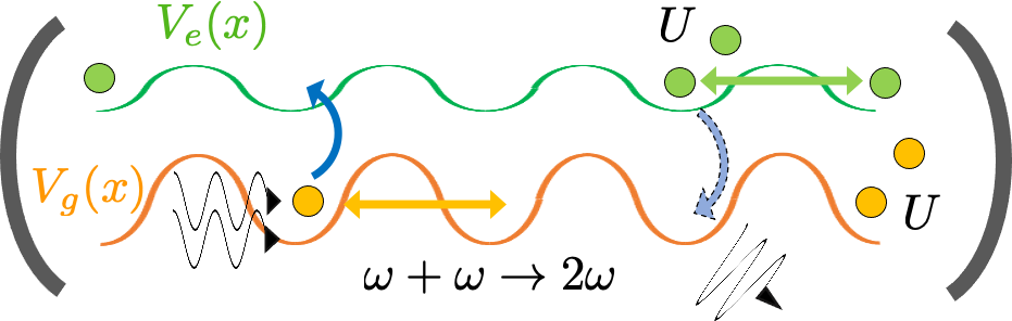
Figure 1: Illustration of the system. The bosonic atoms in the optical lattice experience a different potential $V_{e/g}$ whether they are in an internal ground/excited state. The bare excitation energy $\omega_{eg}$, see Eq. (2) corresponds to the average distance between the two potential profiles. Atoms can hop between lattice sites within a given potential landscape but when at the same lattice site they experience repulsive interactions, as specified in Eq. (6). Absorption and fluorescence occur when the atoms change between landscapes/internal states by emitting/absorbing photons (the case of SHG is schematically shown).

We also express $\hat{\tilde{H}}^{(I)}_{A}$ using the Wannier functions basis and, due to the localised character Wannier functions, we make the approximation that interactions between atoms at different sites can be neglected. With only the intra-atomic density-density contributions retained, we have $\hat{\tilde{H}}^{(I)}_{A}\rightarrow\hat{H}^{(I)}_{A}$, with

$$\!\!\!\!\!\!\!\hat{H}^{(I)}_{A}=\sum_{i}^{L}\bigg{[}\frac{U_{g}}{2}\hat{n}_{i}^{g}(\hat{n}_{i}^{g}-1)+\frac{U_{e}}{2}\hat{n}_{i}^{e}(\hat{n}_{i}^{e}-1)+U_{eg}\hat{n}_{i}^{g}\hat{n}_{i}^{e}\bigg{]},$$ (6)

and where $\hat{n}_{i}^{g/e}$ corresponds to density operator for the the ground/excited atom state at site $i$, and $U_{g},U_{e},U_{eg}$ determine the strength of the different interaction terms.

Moving now to the radiation part of the system, the Hamiltonian $\hat{H}_{R}(t)$ for two photon-modes is given by

$$\hat{H}_{R}(t)=\omega_{0}\hat{b}^{\dagger}\hat{b}+\omega\hat{b}_{f}^{\dagger}\hat{b}_{f}+\hat{H}_{Drive}(t)$$ (7)

where $\hat{b}^{\dagger}$ ($\hat{b}^{\dagger}_{f}$) creates a cavity (fluorescent) photon with frequency $\omega_{0}$ ($\omega$), and $\hat{H}_{Drive}(t)$ represents the possible action of a laser that injects photons in the cavity.

Concerning the Wannier functions, we further assume $\langle\Omega_{g}^{(i)}|\Omega_{e}^{(i)}\rangle\gg\langle\Omega_{g}^{(i)}|\Omega_{e}^{(j)}\rangle$ when $i\neq j$ (which is very often the case), and take into account only intra-site light-induced (de)excitations. Accordingly, the atom-photon interaction Hamiltonian assumes the form

$$\!\!\!\!\!\hat{H}_{AR}(t)=[g_{i}(\hat{b}^{\dagger}+\hat{b})+g^{\prime}(t)(\hat{b}_{f}^{\dagger}+\hat{b}_{f})]\sum_{i}(\hat{\alpha}_{i}^{\dagger}\hat{\beta}_{i}+\textrm{h.c.}).$$ (8)

In Eq. (8), $g_{i}$ is the incident field coupling, and $g^{\prime}(t)=g_{f}e^{-i\Gamma t}$ describes the coupling of the atoms with fluorescent photons, which is initially $g_{f}$ and that then gets attenuated in time. This choice of $g^{\prime}(t)$ is motivated at the end of this section. We note that an atom-photon coupling Hamiltonian similar to Eqs. (1, 5-8), but with only one photon field and $\hat{H}_{AR}$ treated in the rotating wave approximation (RWA), was already considered in e.g. Ref. [31]. To summarize, the final form assumed by the Hamiltonian is

$$\hat{H}(t)=\hat{H}^{0}_{A}+\hat{H}^{I}_{A}+\hat{H}_{R}(t)+\hat{H}_{AR}(t),$$ (9)

with the different terms explicitly specified given by Eqs. (5-8).

The main observable of our study is the fluorescent spectrum of the ultracold-atom system, that is characterised in terms of the probability $\mathcal{S}(t,\omega)$ of observing one or more emitted photons [57, 58]. Such quantity is defined as

$$\mathcal{S}(t,\omega)=\sum_{\lambda n}\sum_{m>0}\rvert\langle\lambda nm|\mathcal{T}\big{[}e^{-i\int_{0}^{t}\hat{H}(t^{\prime})dt^{\prime}}]\big{|}\Phi_{0}\rangle\rvert^{2},$$ (10)

where $\lambda$, $n$, and $m$ respectively label the states corresponding to the atom-, the incident-, and the fluorescent- field, and $|\Phi_{0}\rangle$ is the initial state of the system. Later in the discussion, we will specify the different typed of initial states that are considered in the calculations. Also, we denote by $\mathcal{S}(\omega)$ the long-time, steady-state limit of Eq. (10), to be used later when discussing the results; that is, $\mathcal{S}(\omega)\equiv\mathcal{S}(t\rightarrow\infty,\omega)$.

We employ the short iterated Lanczos algorithm for the exact time evolution of the system. The associated problem size in the space of configurations is $M=M_{B}M_{c}M_{f}$, with $M_{B}$ representing the size of the cold bosonic atom system, and $M_{c}$, and $M_{f}$ respectively denoting the maximum number of incident and fluorescent photons included in the matter+light Fock space. For all calculations in the paper, we set the hopping parameters $t_{g}=t_{e}=t=-0.01$, and the energies $\epsilon_{g}=0.0$ and $\epsilon_{e}=2.0$, i.e. the nominal resonance frequency for the atoms optical transition is $\Omega_{R}=\epsilon_{e}-\epsilon_{g}=2.0$. Furthermore, we choose $\Gamma=0.02$, with the atom-photon coupling constants set to $g_{i}=0.1$ and $g_{f}=0.01$ for the incident and fluorescent fields, respectively. Finally, for the atom-atom interactions, we consider $U_{g}=U_{e}=U$ and $U_{eg}=U/2$, and consider different choices for $U$. We note that the values chosen for the optical lattice parameters and the incident photon couplings correspond to those used in Ref. [31] (after a rescaling of units by a factor 10²), while the chosen average photon number in the cavity, $\langle\hat{b}^{\dagger}\hat{b}\rangle\approx 16$, permits to observe multiphoton effects on the fluorescent spectra while keeping the numerical calculations manageable.

The coupling to the fluorescent field. - Instead of using an exponentially damped $g^{\prime}(t)$ as specified above, dissipation and cavity-leakage could be included via treatments based on e.g. Lindbladh master equations, or non-equilibrium Green’s functions. These approaches can rigorously take into account both radiative and non-radiative damping mechanisms and ensure that, in the long time limit, convergence to a steady-state fluorescent spectrum is attained. In this work, to stay within a wavefunction/configuration interaction scheme, we start by using a phenomenological form of the coupling to the fluorescent field (with a damping rate set by $\Gamma$). Later in the paper, we will introduce a more microscopic characterization of cavity leakage via external baths made of classical harmonic oscillators. System and baths will be described within a mixed quantum-classical scheme that, although approximate, is computationally convenient and ensures a unitary time evolution of the quantum (sub)system wavefunction.

III Second Harmonic generation

As a premise to the characterization of SHG in an ultracold-atom system, it can be useful to consider the effect that photon pumping has on the fluorescent response of a system with resonance frequency $\Omega_{R}$. As shown in a previous work [58], when the material+cavity system is in the ground state and then photons of frequency $\Omega_{R}/2$ are pumped into the cavity at a finite rate, the time dependent SHG signal is strongly hindered. A sizeable SHG signal is however recovered in the limit of ultrafast photon pumping (similarly to what would happen when at $t=0$ the material system is in the ground state and the cavity photons are prepared in a coherent state $|\eta\rangle$ [58]). These overall features of SHG should be contrasted to the case of resonant frequency $\Omega_{R}$ (to be discussed for ultracold atoms in Sec. IV), where a large fluorescent signal is obtained irrespective of how the initial state is prepared [58]).

In line with these considerations, we here induce SHG by considering an incident field frequency $\omega_{0}=\Omega_{R}/2=1.0$. The initial state of the system for the SHG calculations is $|\Phi_{0}\rangle\equiv|\Phi_{0}^{SHG}\rangle=|\phi_{A}\rangle|\eta\rangle|0_{f}\rangle$, which is a product of a cold-atom many-body state and the two photon-field states. We choose $|\phi_{A}\rangle$ as the lowest (ground) energy state of $H_{A}$, while $|\eta\rangle$ is a coherent state representing the initial state of the incident field and $|0_{f}\rangle$ is the vacuum state of the fluorescent field. All the SHG calculations in this section are obtained with $\langle\hat{b}^{\dagger}\hat{b}\rangle=\eta^{2}=16$.

Figure 2: SHG signal in the long time limit as function of chain size $L$, atom number $N_{a}$ and atomic interaction $U$. For all cases, the initial state is $|\Phi_{0}^{SHG}\rangle$, $U_{eg}=U/2$, $\eta=4.0$, and $\omega_{0}=1.0$. Panel $\bm{(a)}$: $U=0.0001$. Panel $\bm{(b,c,d)}$: $U=5.0$.

Low vs high interactions, number of atoms vs sites.- The ultracold boson systems in optical lattices studied in this work are small chains with $L=2,3,4$ sites, two orbitals/site and $N_{a}=1,2,...,5$ particles. We generally use a maximum of $N_{0}=59$ incident and $N_{f}=4$ fluorescent photons. Thus, the size of the total configuration space is ${2L+N_{a}-1}\choose N_{a}$ $N_{0}N_{f}$. Finally, to produce a fluorescent spectrum $\mathcal{S}(t,\omega)$ (or $\mathcal{S}(\omega)$ in the long time limit), we use a grid with $N_{\omega}=150$ points for the frequency $\omega$.

Not all the possible combinations of the above $L,N_{a}$ parameters are explicitly considered in the paper. In fact, a large fraction of the presented results is for $L=2$ because, as it will become evident from the cases presented, the $L=2$ system already displays many of the qualitative trends exhibited at larger $N$ and larger $L$, while being computationally very convenient (additional results with larger $L$ can be found in Appendix A).

The changes in the SHG signal due to variations in atom-atom interaction, number of atoms, and sites are shown in Fig. 2. In the low interaction regime ($U=0.0001$), when increasing the number of atoms the intensity of $\mathcal{S}(\omega)$ also increases (Fig. 2a). This is a simple cumulative effect. With essentially no hindrance from the interactions, i.e. the atoms basically independent from each other, the number the intrasite excitations increases without constraints, and so does the SHG signal. For the same reason, increasing the number of sites has also a negligible effect on the fluorescent spectra in the low interaction regime, as it can be seen in Appendix A (Fig. 12).

The situation changes in the high interaction regime ($U=5$), as shown in Fig. 2b-d. In this case, increasing the number of atoms will enhance the intensity of the fluorescent spectrum until $N_{a}\leq L$, very similarly to the low interaction regime. However, when $N_{a}>L$, we observe a decline in the intensity of $\mathcal{S}(\omega)$, and in many cases the SHG peak is reduced. This is because for $N_{a}>L$ there is an increased interaction penalty for having on average more than one-excited atom at each site.

Figure 3: Results are of total excited atoms $\mathcal{D}_{e}$ as a function of time and for different interaction strengths. Panel $\bm{(a)}$: $U=0.0001$; Panel $\bm{(b)}$: $U=5.0$. In all calculations, $L=2$, $U_{eg}=U/2$, $\eta=4.0$, $\omega_{0}=1.0$ and the initial state is $|\Phi_{0}^{SHG}\rangle$.

To scrutinise this interpretation, we plot in Fig. 3 the total number of excited atoms $\mathcal{D}_{e}=\sum_{i}^{L}\langle\hat{n}_{i}^{e}\rangle$ as a function of time. At low interactions, (Fig. 3a) there is a large variation at early times in $\mathcal{D}_{e}$ as we increase $N_{a}$. But for $N_{a}>L$ and high interactions(Fig. 3b), the atoms already present in the excited state at time $t=0.0$ somewhat prevent further excitations, i.e. a relatively smaller change in $\mathcal{D}_{e}$ is observed, before the photon pumping ceases and/or the coupling with the fluorescence fields is significantly attenuated.

Another interesting feature to be noted for non small interactions and $N_{a}>L$ is the presence of significant fluorescent spectral weight at very low frequencies (the broad shoulder well below the incident frequency $\omega_{0}=1$ in Fig. 2b-d). This again is related to the role of interactions: with these presents, the energy spectrum of the many-atom system acquires a fine structure with several low-lying states which can be reached via optical excitation from the ground state.

Intermediate interaction strength.- The two regimes considered so far correspond to somewhat extreme values in the atom-atom interaction range. A scan of the related interaction interval is provided in Fig. 4$\bm{(a)}$, where, on increasing the interaction, the spectral intensity decreases and the SHG peak gets split and shifted. The corresponding behavior of the total number of excited atoms $\mathcal{D}_{e}$ in Fig. 4$\bm{(b)}$ confirms that interactions hinder the transition between the ground and the excited atomic states. Interestingly, the small variation in $\mathcal{D}_{e}$ after the initial excitation spikes suggests that such hindrance remains even though the excited levels are scarcely populated.

Figure 4: Results are of intermediate interactions. Panel $\bm{(a)}$ shows the fluorescent spectra, and $\bm{(b)}$ contains plot of number of excited atoms $\mathcal{D}_{e}$ as a function of time. In all calculations $L=2$, $N_{a}=3$, $U_{eg}=U/2$, $\eta=4.0$, $\omega_{0}=1.0$ and the initial state is $|\Phi_{0}^{SHG}\rangle$.

IV Resonance calculations

The other regime we consider in this work is the resonant one, i.e. $\omega_{0}=\Omega_{R}$. As mentioned at the beginning of Sect. III, the intensity of the SHG signal in the low-photon regime decays very fast on decreasing the pumping speed of photons in the cavity, and this motivated our preparation of the pump field in a coherent state at $t=0$ in Sect. III. At resonance, however, the overall intensity of the fluorescent response has a considerably milder dependence on the photon ramping speed [57, 58]. Because of this, in this section we drive the resonant field at a finite ramping rate, which in principle also makes possible to characterize the system’s response during the driving.

With this prescription, the initial state of the systems $|\Phi_{0}\rangle\equiv|\Phi_{0}^{Res}\rangle$ is chosen as the exact ground state of the full Hamiltonian $H(t=0)$, where atoms and cavity are initially in mutual equilibrium and the average photon number is nearly zero. The dynamics is then started with injecting photons in the cavity via an external laser pulse, considering an additional drive term $\hat{H}_{Drive}(t)$ in the Hamiltonian in Eq. (9), given by

$$\hat{H}_{Drive}(t)=g_{d}(\hat{b}+\hat{b}^{\dagger})[f(t)\sin(\omega_{0}t)],$$ (11)

and where $f(t)$ is a smoothed rectangular envelope. Explicitly, $f(t)=[1-\mathcal{F}_{1}(t)]\mathcal{F}_{2}(t)$, with $\mathcal{F}_{i}(t)=[\exp((t-t_{i})/\tau_{i})+1]^{-1}$. This corresponds to a laser-cavity coupling in the time interval $(t_{1},t_{2})$. In the simulations, $\tau_{1}=\tau_{2}=2.0$, $t_{1}=\frac{6\pi}{\omega_{0}}$, $t_{2}=\frac{31\pi}{\omega_{0}}$) while $g_{d}$, the laser driving strength, is tuned in such a way that the number of incident photons $\langle\hat{b}^{\dagger}\hat{b}\rangle\approx 16.0$ at the end of the drive.

Low vs high interactions, number of atoms vs sites.- Resonant fluorescence results for $L=2$ and different $N_{a}$, and for both low and high interaction strength, are reported in Fig. 5. As for the SHG case, at low interactions (panel a) increasing the particle number boosts the intensity of the fluorescent spectrum. The dependence of $S(\omega)$ on $N_{A}$ is however non monotonic at large interactions (panel b). Interestingly, the Mollow sidebands (typical of the resonance signal) are noticeably hindered. This behavior, due to the photons being introduced in the cavity via finite-time driving, is also observed for other values of $L$ and $N_{a}$ (see Fig. 14 in Appendix B). As another consequence of a non-instantaneous photon pumping, in Fig. 5 there is no broad shoulder in the spectrum at low frequencies. To elaborate on this observation, in Appendix B we also show results for $L=2$ and $N_{a}=3,4,5$, but with the cavity field initially prepared in a coherent state. For such ”instantaneous” drive, there are peaks at the low end of the spectrum (Fig. 15), in contrast to what happens in Fig. 5 at finite pumping rate.

Figure 5: Resonant fluorescence spectra in a dimer ($L=2$) for varying number of atoms $N_{a}$ and atomic interaction $U$ (in all cases, $U_{eg}=U/2$) Panels $\bm{(a)}$ and $\bm{(b)}$ show results for $U=0.0001$ and $U=5.0$, respectively. In all cases, $\omega_{0}=2.0$, $\tau_{1}=\tau_{2}=2.0$, $t_{1}=\frac{6\pi}{\omega_{0}}$, $t_{2}=\frac{31\pi}{\omega_{0}}$. The initial state is $|\Phi_{0}^{Res}\rangle$. The value of the external laser field coupling $g_{d}$ is determined in such a way that the number of incident photons $\langle\hat{b}^{\dagger}\hat{b}\rangle\approx 16.0$ at the end of the drive.

The overall behavior of the resonant fluorescence spectra just discussed is to be ascribed (as for SHG) to the effect of the interactions and the amount of atoms in the system. In Fig. 6, we report the behavior of $\mathcal{D}_{e}=\sum_{i}^{L}\langle\hat{n}_{i}^{e}\rangle$. Up to $N_{a}=3$, $\mathcal{D}_{e}$ evolves in time very much in the same way for low and high interactions (i.e., interactions basically play no role). For larger number of atoms, this is not the case: for strong interactions the atoms tend to occupy the excited state already at time $t=0$, hampering (as in SHG case) further excitations.

Since in the resonant case we ramp photons into the cavity via an external driving field, we can further characterize the situation by looking at the value of the drive coupling $g_{d}$. At low interactions, to have $\langle\hat{b}^{\dagger}\hat{b}\rangle\approx 16$ at the end of the drive, the needed value of $g_{d}$ increases as $N_{a}$ becomes larger (Fig. 6a). That is, with more atoms in the systems, more transitions occur and more photons need to be introduced during the drive (i.e. a higher $g_{d}$ is needed). On the other hand, for strong interactions, $g_{d}$ will not always need to be increased as $N_{a}$ gets larger (the $g_{d}$ value is low for $N_{a}=3$ and $N_{a}=4$). In these cases, there is less absorption of the incident photons during the drive, and the corresponding fluorescent spectra are less intense (Fig. 5b).

Figure 6: Total number of excited atoms $\mathcal{D}_{e}$ (see main text) as a function of time for the regime of resonant fluorescence. In all cases, the initial state is chosen as $|\Phi_{0}^{Res}\rangle$, $U_{eg}=U/2$, $L=2$, $\omega_{0}=2.0$, $\tau_{1}=\tau_{2}=2.0$, $t_{1}=\frac{6\pi}{\omega_{0}}$, and $t_{2}=\frac{31\pi}{\omega_{0}}$. Panel $\bm{(a)}$: weak interaction regime ($U=0.0001$); Panel $\bm{(b)}$: strong interaction regime ($U=5.0$). The value of $g_{d}$ is determined in such a way that the number of incident photons $\langle\hat{b}^{\dagger}\hat{b}\rangle\approx 16.0$ at the end of the drive.

Intermediate interaction strength.- In Fig. 7, we report the case of interactions of intermediate strength, again for $L=2$ and all the other parameters specified as before. Not unexpectedly, the intensity of the resonant fluorescent spectrum monotonically decreases as the interaction increases (Fig. 7a). Additionally, the results for the time evolution of $\mathcal{D}_{e}$ (Fig. 7b) reveal a quite interesting feature when $U=3.0$, namely a plateau in the time-increasing population of the excited state. While being rather sensitive to the values of the parameters in the model, this feature again is a clear marker of the opposition exerted by the already excited atoms to further excitations.

Figure 7: Results are of resonance calculations with intermediate interactions. Panel $\bm{(a)}$ shows the fluorescent spectra, and $\bm{(b)}$ contains plot of number of excited atoms $\mathcal{D}_{e}$ as a function of time. In all calculations $L=2$, $N_{a}=3$, $U_{eg}=U/2$, $\omega_{0}=2.0$, $\tau_{1}=\tau_{2}=2.0$, $t_{1}=\frac{6\pi}{\omega_{0}}$, $t_{2}=\frac{31\pi}{\omega_{0}}$ and the initial state is $|\Phi_{0}^{Res}\rangle$. The value of $g_{d}$ is chosen such that $\langle\hat{b}^{\dagger}\hat{b}\rangle\approx 16.0$ at the end of the drive.

V Cavity leakage with classical oscillator baths

We now allow for the possibility of an imperfect cavity and, to simulate leakage losses, we make the cavity photons to interact with (and possibly be removed by) a bath of harmonic oscillators, To this end, we follow the prescription used to describe a bath interacting with a single quantum mode (see e.g. Ref. [36]) but, dealing with two quantum modes, we introduce a distinct bath for each of them. Explicitly, we augment the Hamiltonian of Eq. (9) as $\hat{H}(t)\rightarrow\hat{H}(t)+\hat{H}_{Loss}$, with

$$\hat{H}_{Loss}=\sum_{k=1}^{\mathcal{N}_{K}}\bigg{[}\frac{\hat{p}^{2}_{k}}{2}+\frac{\omega^{2}_{k}}{2}\bigg{(}\hat{x}_{k}-\frac{C_{k}}{\omega^{2}_{k}}(\hat{b}^{\dagger}+\hat{b})\bigg{)}^{2}\bigg{]}$$

$$+\sum_{j=1}^{\mathcal{N}_{J}}\bigg{[}\frac{\hat{p}^{2}_{j}}{2}+\frac{\omega^{2}_{j}}{2}\bigg{(}\hat{x}_{j}-\frac{C_{j}}{\omega^{2}_{j}}(\hat{b}_{f}^{\dagger}+\hat{b}_{f})\bigg{)}^{2}\bigg{]},$$ (12)

with $\mathcal{N}_{K/J}$ the number of classical oscillators for bath $K/J$ (each of them with coordinates ($p_{k/j},x_{k/j}$), unit masses $m_{k/j}=1$ and frequency $\omega_{k/j}$), and where $\{C_{k/j}\}$ determine the bath-photon coupling strengths for the incident/fluorescent field. Cavity leakage is thus included via a Caldeira-Leggett-type description [59, 60, 58].

To detail the role of the bath(s), we expand the terms which are quadratic in the bath coordinates, and rewrite Eq. (12) as $\hat{H}_{Loss}=\sum_{i=1}^{4}\hat{H}^{(i)}_{L}$, where

$$\hat{H}^{(1)}_{L}=\frac{1}{2}\sum_{k=1}^{\mathcal{N}_{K}}\left({\hat{p}_{k}^{2}}+\omega_{k}^{2}\hat{x}_{k}^{2}\right)+\frac{1}{2}\sum_{j=1}^{\mathcal{N}_{J}}\left({\hat{p}_{j}^{2}}+\omega_{j}^{2}\hat{x}_{j}^{2}\right)$$ (13)

$$\hat{H}^{(2)}_{L}=-\sum_{k=1}^{\mathcal{N}_{K}}{C}_{k}\hat{x}_{k}(\hat{b}^{\dagger}+\hat{b})-\sum_{l=j}^{\mathcal{N}_{J}}{C}_{j}\hat{x}_{j}(\hat{b}_{f}^{\dagger}+\hat{b}_{f})$$ (14)

$$\hat{H}^{(3)}_{L}=\sum_{k=1}^{\mathcal{N}_{K}}\frac{C_{k}^{2}}{\omega_{k}^{2}}\hat{b}^{\dagger}\hat{b}+\sum_{j=1}^{\mathcal{N}_{J}}\frac{C_{j}^{2}}{\omega_{j}^{2}}\hat{b}_{f}^{\dagger}\hat{b}_{f}$$ (15)

$$\hat{H}^{(4)}_{L}=\sum_{k=1}^{\mathcal{N}_{K}}\frac{C_{k}^{2}}{2\omega_{k}^{2}}(\hat{b}^{\dagger})^{2}+\sum_{j=1}^{\mathcal{N}_{J}}\frac{C_{j}^{2}}{2\omega_{j}^{2}}(\hat{b}_{f}^{\dagger})^{2}+\textrm{h.c}.$$ (16)

We can thus see that $\hat{H}^{(1)}_{L}$ describes the independent bath oscillators, $\hat{H}^{(2)}_{L}$ accounts for the photon-bath interaction, $\hat{H}^{(3)}_{L}$ renormalises the photon frequencies, and $\hat{H}^{(4)}_{L}$ induces fluctuations in the photon number.

Figure 8: Cavity leakage and SHG. Panels $(\bm{a})$ to $(\bm{d})$: The spectra in the presence of leakage are given by the 3D time evolving plots, whilst the red curves describe SHG in the long time limit and without leakage. For the baths parameters, we set ${C}_{k}=A(\Delta k)^{a}$ and ${C}_{j}=A(\Delta j)^{a}$, with $A=0.005$, $a=0.6$, $\Delta=0.01$ and $\mathcal{N}_{K/J}$=1000. In all calculations, $L=2$, $U_{eg}=U/2$, $\eta=4.0$, $\omega_{0}=1.0$, and the initial state is $|\Phi_{0}^{SHG}\rangle$. Panels $(\bm{a,b})$ refer to $U=0.0001$, whereas $(\bm{c,d})$ are for $U=5.0$. Panel $\bm{(e)}$: average photon $\langle\hat{b}^{\dagger}\hat{b}\rangle$ of the incident field in the presence of leakage.

Figure 9: Cavity leakage and resonant fluorescence. Panels $(\bm{a})$ to $(\bm{d})$: The spectra in the presence of leakage are given by the 3D time evolving plots, whilst the red curves describe resonant spectrum in the long time limit and without leakage. For the baths parameters, we set ${C}_{k/j}=A(\Delta(k/j)^{a}$, with $A=0.005$, $a=0.6$, $\Delta=0.01$ and $\mathcal{N}_{K/J}$=1000. In all calculations, $L=2$, $U_{eg}=U/2$, $\eta=4.0$, $\omega_{0}=2.0$, and the initial state is $|\Phi_{0}^{Res}\rangle$. Panels $(\bm{a,b})$ refer to $U=0.0001$, whereas $(\bm{c,d})$ are for $U=5.0$. Panel $\bm{(e)}$: average photon $\langle\hat{b}^{\dagger}\hat{b}\rangle$ of the incident field in the presence of leakage. The value of $g_{d}$ is determined by requiring that it the absence of leakage, $\langle\hat{b}^{\dagger}\hat{b}\rangle\approx 16$ at the end of the ramping.

The treatment of $\hat{H}_{Loss}$ should in principle be fully quantum-mechanical. However, to stay in a wavefunction description for the atoms+cavity system which is exact, unitary, and numerically viable, we use the Ehrenfest dynamics, where the bath degrees of freedom are treated classically, i.e. $\{\hat{x}_{k},\hat{x}_{j},\hat{p}_{k},\hat{p}_{j}\}\rightarrow\{x_{k},x_{j},p_{k},p_{j}\}$. Thus, $\ddot{x}_{\mu}(t)=-\omega_{\mu}^{2}x_{\mu}(t)+C_{\mu}\langle\hat{b}_{\mu}^{\dagger}+\hat{b}_{\mu}\rangle_{\bar{x},t}$, where $\bar{x}=\{x_{k}\}\cup\{x_{j}\}$, and $\mu\in[1,\mathcal{N}_{K}]$ with $\hat{b}_{\mu}=b$ or $\mu\in[1,\mathcal{N}_{J}]$ with $\hat{b}_{\mu}=b_{f}$.

In general, the Ehrenfest dynamics incorrectly accounts for detailed balance, as e.g. shown for electron-nuclei [61], electron-spin [62, 63], and spin-spin systems [64]. Though, it gives a fair treatment when the system’s trajectory occurs near a single potential energy surface [65]. We anticipate similar scenarios for photons interacting with classical Caldeira-Leggett’s oscillators. Since our aim here is to describe qualitative trends in SHG for weak cavity leakage (but beyond a phenomenological damping correction), a quantitatively inaccurate detailed balance is not expected to be of central relevance.

For the calculations with leakage effects included, we consider the same bath coupling strength for both fields, i.e., ${C}_{j}={C}_{k}$ for $j=k$, with $\mathcal{N}_{J}=\mathcal{N}_{K}=1000$ and ${C}_{k}=A(\omega_{k})^{a}$ with $\omega_{k}=\Delta k$. Hence, the photon damping rate is determined by the parameters $A$, $a$, and $\Delta$ which, for the results presented, take the value $A=0.005$, $a=0.6$, $\Delta=0.01$, giving a maximum oscillator frequency $\omega_{Max}=10$.

Results in the SHG and resonant regimes.- The SHG spectra for $L=2$ and two different number of atoms $N_{A}$ are shown in Fig. 8(panels a-d), where the time-evolving surface plots are with cavity leakage included, and the orange curves correspond to the long-time limit spectra without leakage. Not unexpectedly, the results show that cavity leakage overall reduces the spectral intensity (along with this reduction, the SHG peak is also slightly redshifted). This is confirmed by the behavior of $\langle\hat{b}^{\dagger}\hat{b}\rangle$ in Fig. 8$\bm{(e)}$, showing that the number of photons decreases in time due to leakage, making less effective the excitation process.

Results for the resonant regime are reported in Fig. 9 (panes a-d). In this case, the dynamics is induced by ramping the cavity field, with full system+cavity+bath initially in the ground state (in this state, the average number of incident photons $\langle\hat{b}^{\dagger}\hat{b}\rangle\simeq 0$ at $t=0$.) At resonance too, cavity leakage decreases the intensity of the fluorescent spectra. It is useful to analyse this behavior in terms of $\langle\hat{b}^{\dagger}\hat{b}\rangle$ (Fig. 9$\bm{(e)}$). Comparing $\langle\hat{b}^{\dagger}\hat{b}\rangle$ from panels a,b) and from panels c,d), we clearly note a larger role played by leakage when the atom-atom interaction is stronger: at the same time, a stronger Hubbard repulsion hinders the atom excitation to the higher levels, the number of photons in the cavity is much more reduced due to leakage, and less absorption of the incident photons occurs. That is, the fluorescence response is reduced.

VI Fluorescence from a two-component BEC

Until now, our discussion has been devoted to fluorescence in 1D Bose-Hubbard optical lattices with weak/strong inter-particle correlations, and with/without radiation leakage from the cavity. By using an exact CI approach, we were limited to rather small clusters and number of particles (Sects. II-V).

To consider a case where size effects are mitigated, we now address the fluorescent response from ultracold bosons in the condensed phase, and in the large $N$-limit [66]. To maintain a simple level of description, we will examine a finite-but-large-$N$ sample of two-component bosons in a trapped geometry, and in the Bose-Einstein condensate (BEC) regime. The system we study and the description we employ are rather standard in BEC research, and in what follows we just summarize the main steps leading to our system+cavity Hamiltonian, referring to the literature for details.

Our system is made of $N$ bosonic atoms with two internal states labeled $e,g$. Depending on their internal state, the atoms experience different trapping potentials (as before, denoted by $V_{g}$ and $V_{e}$, respectively). We assume that the system is weakly interacting, in the dilute limit, and at low temperature (where thermal excitations and condensate depletion are usually deemed negligible). This allows us to approximate the inter-particle interactions among same and different internal states via effective contact interactions (whose strengths are related to respective the s-wave scattering lengths).

Under these specifications, the two-component BEC (2BEC) Hamiltonian can be written as [20, 67]

$$\hat{H}_{2BEC}=\sum_{\kappa\in\{g,e\}}\int d{\bf x}~{}\hat{\psi}_{\kappa}^{\dagger}({\bf x})\big{[}-\frac{\hbar^{2}\nabla^{2}}{2m}+V_{\kappa}({\bf x})\big{]}\hat{\psi}_{\kappa}({\bf x})$$

$$+\sum_{\kappa,\kappa^{\prime}\in\{e,g\}}\int d{\bf x}~{}\hat{\psi}_{\kappa}^{\dagger}({\bf x})\hat{\psi}_{\kappa^{\prime}}^{\dagger}({\bf x})\mathcal{U}_{\kappa\kappa^{\prime}}\hat{\psi}_{\kappa^{\prime}}({\bf x})\hat{\psi}_{\kappa}({\bf x}),$$ (17)

where $\mathcal{U}_{gg}~{}(\mathcal{U}_{ee}$) is the interaction strength (related to the scattering length) for atoms of the same state $g$ ($e$), and $\mathcal{U}_{ge}=\mathcal{U}_{eg}$ is the interaction strength for atoms of different states. In addition, under the same assumptions, it possible to introduce a further approximation, i.e. the field operators are expressed as $\hat{\psi}^{\dagger}_{g}({\bf x})\approx\phi_{g}({\bf x})\hat{\alpha}^{\dagger}$, $\hat{\psi}^{\dagger}_{e}({\bf x})\approx\phi_{e}({\bf x})\hat{\beta}^{\dagger}$, where $\phi_{\kappa=g/e}$ is the eigenstate of lowest energy satisfying

$$\big{[}-\frac{\hbar^{2}\nabla^{2}}{2m}+V_{g/e}({\bf x})\big{]}\phi_{g/e}({\bf x})=E_{g/e}\phi_{g/e}({\bf x}),$$ (18)

and $E_{e}>E_{g}$. Inserting the field operators in Eqs. (VI,18), performing the space-integrations, and absorbing inherent constants and parameters (e.g., the scattering lengths) into the interaction terms $U_{\kappa\kappa^{\prime}}$, we obtain

$$\hat{H}_{2BEC}=E_{g}\hat{\alpha}^{\dagger}\hat{\alpha}+E_{e}\hat{\beta}^{\dagger}\hat{\beta}$$

$$+\frac{1}{2}U_{gg}(\hat{\alpha}^{\dagger})^{2}\hat{\alpha}^{2}+\frac{1}{2}U_{ee}(\hat{\beta}^{\dagger})^{2}\hat{\beta}^{2}+U_{eg}\hat{\alpha}^{\dagger}\hat{\alpha}\hat{\beta}^{\dagger}\hat{\beta}.$$ (19)

Finally, to consider the BEC-cavity interaction, we proceed as discussed in Refs. [20, 67, 68, 37]). Accordingly, in the dipole approximation, with two optical modes with frequency $\omega_{0}$ and $\omega_{f}$, the Hamiltonian term describing the light-2BEC coupling assumes the form (for the possible inclusion of higher-order terms in the cavity-2BEC interaction, see e.g. [37])

$$\hat{H}^{\prime}=(\hat{\alpha}^{\dagger}\hat{\beta}+\hat{\beta}^{\dagger}\hat{\alpha})\big{[}g_{i}(\hat{b}^{\dagger}+\hat{b})+g_{f}(\hat{b}_{f}^{\dagger}+\hat{b}_{f})\big{]},$$ (20)

where the space dependence of the field(s) is absorbed in the coupling constants. Putting all the contributions together, the total 2BEC+cavity Hamiltonian is

$$\!\!\!\!\!\!\hat{H}_{2BEC} =E_{g}\hat{\alpha}^{\dagger}\hat{\alpha}+E_{e}\hat{\beta}^{\dagger}\hat{\beta}+\omega_{0}\hat{b}^{\dagger}\hat{b}+\omega_{f}\hat{b}_{f}^{\dagger}\hat{b}_{f}$$

$$+\frac{1}{2}U_{gg}(\hat{\alpha}^{\dagger})^{2}\hat{\alpha}^{2}+\frac{1}{2}U_{ee}(\hat{\beta}^{\dagger})^{2}\hat{\beta}^{2}+U_{eg}\hat{\alpha}^{\dagger}\hat{\alpha}\hat{\beta}^{\dagger}\hat{\beta}$$

$$+(\hat{\alpha}^{\dagger}\hat{\beta}+\hat{\beta}^{\dagger}\hat{\alpha})\big{[}g_{i}(\hat{b}^{\dagger}+\hat{b})+g_{f}(t)(\hat{b}_{f}^{\dagger}+\hat{b}_{f})\big{]}.$$ (21)

We will use $\hat{H}_{2BEC}$ for repulsive interactions, deferring the attractive case to future work. Differently from what is often assumed in the literature, no use is made here of the RWA in $\hat{H}_{2BEC}$, and the two (cavity and fluorescent) modes are treated both quantum mechanically. Furthermore, and as motivated earlier in the paper, we again consider a damped coupling constant $g_{f}(t)=g_{0}\exp(-\Gamma t)$ for the fluorescent field.

With Eq. (VI), we can directly deal with systems with a finite (albeit, in principle, arbitrarily large) number of particles. However, in the literature, to directly address the macroscopic case, a Bogoliubov approximation (BA) is often performed for the $g$ state. With the BA, it is assumed that the average particle number in the $g$ state, $N_{g}=\langle\hat{\alpha}^{\dagger}\hat{\alpha}\rangle$, remains approximately constant (since $N_{g}$ is large), and one can perform the replacement $\hat{\alpha}^{\dagger}\approx\sqrt{N_{g}},~{}\hat{\alpha}\approx\sqrt{N_{g}}$ in Eq. (VI). The latter then assumes the form

$$\hat{H}^{(BA)}_{2BEC}=\big{[}E_{g}N_{g}+\frac{1}{2}U_{gg}N_{g}(N_{g}-1)\big{]}$$

$$+\big{[}(E_{e}+U_{eg}N_{g})\hat{\beta}^{\dagger}\hat{\beta}+\frac{1}{2}U_{ee}(\hat{\beta}^{\dagger})^{2}\hat{\beta}^{2}\big{]}+\omega_{0}\hat{b}^{\dagger}\hat{b}+\omega_{f}\hat{b}_{f}^{\dagger}\hat{b}_{f}$$

$$+\sqrt{N_{g}}(\hat{\beta}^{\dagger}+\hat{\beta})\big{[}g_{i}(\hat{b}^{\dagger}+\hat{b})+g_{f}(t)(\hat{b}_{f}^{\dagger}+\hat{b}_{f})\big{]}.$$ (22)

The Hamiltonian of Eq.( VI), which corresponds to three mutually interacting boson fields, does not conserve the total number of ultracold boson atoms. A possible way to milden this issue is to assume that particle number conservation in time occurs on average, i.e. $N_{g}(t)+\langle\hat{\beta}^{\dagger}\hat{\beta}\rangle_{t}=N$, with $N$ constant. With this constraint,

$$\!\!\!\!\hat{H}^{(BA)}_{2BEC}\rightarrow\hat{H^{\prime}}^{(BA)}_{2BEC}=E_{g}N_{g}(t)+\frac{1}{2}U_{gg}N_{g}(t)(N_{g}(t)-1)$$

$$\!\!\!\!+\biggl{\{}\big{[}E_{e}+U_{eg}N_{g}(t)\big{]}\hat{\beta}^{\dagger}\hat{\beta}+\frac{1}{2}U_{ee}(\hat{\beta}^{\dagger})^{2}\hat{\beta}^{2}\biggl{\}}+\omega_{0}\hat{b}^{\dagger}\hat{b}+\omega_{f}\hat{b}_{f}^{\dagger}\hat{b}_{f}$$

$$\!\!\!\!+\sqrt{N_{g}(t)}(\hat{\beta}^{\dagger}+\hat{\beta})\big{[}g_{i}(\hat{b}^{\dagger}+\hat{b})+g_{f}(t)(\hat{b}_{f}^{\dagger}+\hat{b}_{f})\big{]},$$ (23)

where $N_{g}(t)=N-\langle\hat{\beta}^{\dagger}\hat{\beta}\rangle_{t}$. In this way, some of the Hamiltonian parameters become time-dependent due to the time-varying average occupation $n_{\beta}(t)\equiv\langle\hat{\beta}^{\dagger}\hat{\beta}\rangle_{t}$ of the excited condensate state. We will not present numerical results based on Eqs. (VI, VI). Yet, these equations show how a renormalization of the effective Hamiltonian parameters actually takes place on varying the particle number $N$. This aspect becomes relevant when comparing results for different 2BEC sizes obtained via Eq. (VI).

Details of the numerical simulations.- Concerning the actual numerical simulations, we will always consider an initial state of the form $|\Psi(0)\rangle=|\eta\rangle|0_{f}\rangle|\Phi_{BEC}\rangle$, where $|\eta\rangle$ is a coherent state for the cavity photons with average number of photons $\eta^{2}$, and $|0_{f}\rangle$ is the vacuum of the fluorescent mode. In turn, $|\Phi_{2BEC}\rangle$ is the ground state of the BEC system when matter and light are uncoupled and where, for all results presented $U_{ee}=U_{gg}=2U_{eg}$. In the case of Eq. (VI), it is seen by inspection that the 2BEC ground state $|\Phi_{2BEC}\rangle$ is always such that $n_{\beta}(0)=0$. On the other hand, for Eq. (VI), how the excited state is occupied depends on the interaction strength: though, it can be shown that when $\max\{U_{gg},U_{ee},U_{eg}\}\ll E_{e}-E_{g}$ (as in our simulations), the ground state is still a $|\Phi_{BEC}\rangle$ with all bosons in the $E_{g}$ state, i.e. $\langle\hat{\beta}^{\dagger}\hat{\beta}\rangle_{t=0}=0$.

Scaling for different particle numbers.- To have a consistent way to compare results for different number of particles, the BEC Hamiltonian is rewritten as follows:

$$\hat{H}=E_{g}\hat{\alpha}^{\dagger}\hat{\alpha}+E_{e}\hat{\beta}^{\dagger}\hat{\beta}+\frac{U_{g}}{2N_{a}}\hat{\alpha}^{\dagger}\hat{\alpha}^{\dagger}\hat{\alpha}\hat{\alpha}+\frac{U_{e}}{2N_{a}}\hat{\beta}^{\dagger}\hat{\beta}^{\dagger}\hat{\beta}\hat{\beta}$$

$$+ \frac{U_{eg}}{N_{a}}\hat{\beta}^{\dagger}\hat{\alpha}^{\dagger}\hat{\alpha}\hat{\beta}+\omega_{0}\hat{b}^{\dagger}\hat{b}+\omega\hat{b}_{f}^{\dagger}\hat{b}_{f}$$

$$+ \frac{g_{i}}{\sqrt{N_{a}}}(\hat{b}^{\dagger}+\hat{b})(\hat{\alpha}^{\dagger}\hat{\beta}+\textrm{h.c.})+\frac{g_{0}e^{-\Gamma t}}{\sqrt{N_{a}}}(\hat{b}_{f}^{\dagger}+\hat{b}_{f})(\hat{\alpha}^{\dagger}\hat{\beta}+\textrm{h.c.}).$$ (24)

In the calculations, the atom-atom interactions $U_{g}/N_{a}=U_{e}/N_{a}=U$ and $U_{eg}/N_{a}=U/2.0$. Similarly to what is usually done for the Dicke model [69, 70], the interactions and the photon field couplings are thus scaled by the number of atoms [38], which also prevents the spectral intensity from diverging in the thermodynamic limit [71].

SHG spectra.- The fluorescent spectra from two 2BEC in the SHG regime, and with respectively $N_{A}=40$ and $N_{A}=400$ atoms, are shown in Fig. 10. The figure also illustrates the dependence of the fluorescent signal on the strength of the cavity-2BEC coupling $g_{i}$ and on the atom-atom interaction $U$ (the dashed curves corresponding to calculations with $U\neq 0$). At low cavity coupling ($g_{i}=0.1$) the spectra with different $N_{a}$ (red and brown solid and dashed curves, see figure for color coding) are almost identical, for both zero and nonzero interactions.

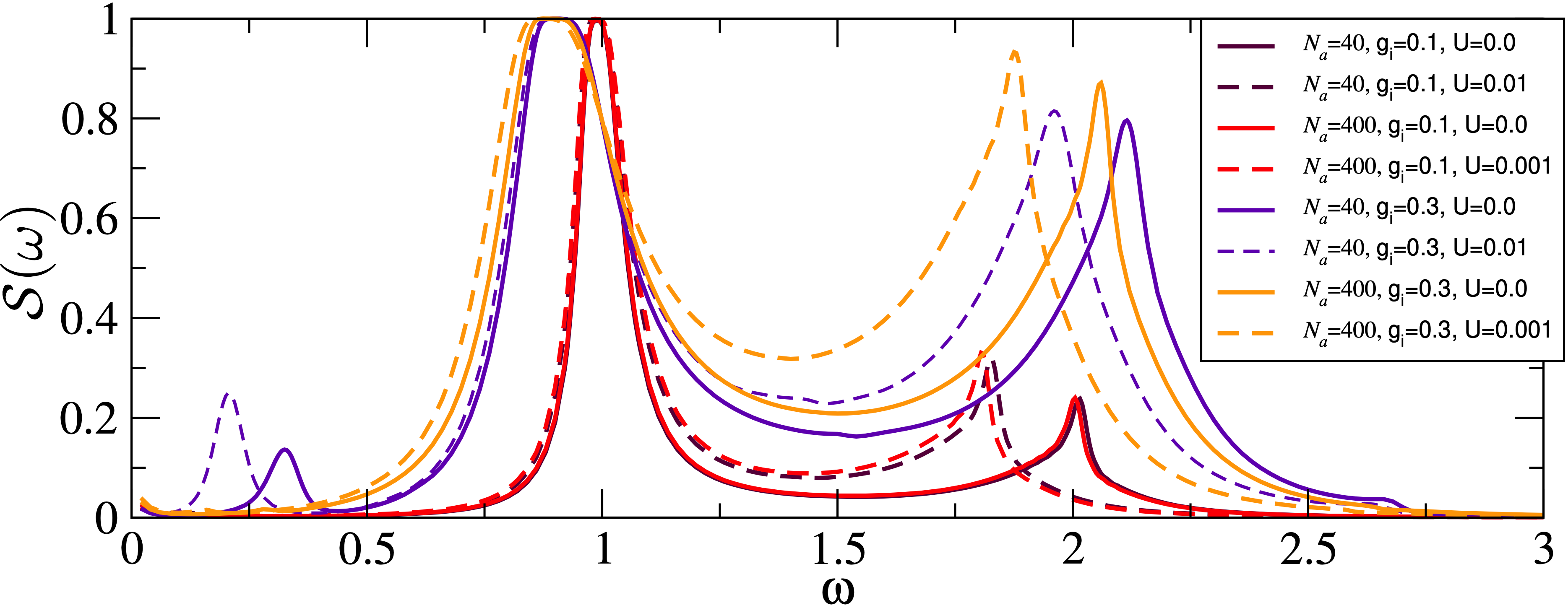
Figure 10: SHG results obtained with an initial coherent photon state with $\langle\hat{b}^{\dagger}\hat{b}\rangle=16$ and $\omega_{0}=1.0$. The parameters used are $U_{g}/N_{a}=U_{e}/N_{a}=U$ and $U_{eg}/N_{a}=U/2.0$, $g_{f}=0.1$, $\Gamma=0.02$, $E_{g}=0.0$ and $E_{e}=2.0$.

We also note that, irrespective of the number of particles, the SHG peak is redshifted for nonzero interactions. The situation changes for larger coupling: at $g_{i}=0.3$ (orange and violet curves), the spectra for $N_{a}=40$ and $N_{a}=400$ markedly differ from each other. Furthermore, there is a significant difference between the results obtained with and without atom-atom interactions. Also, the redshift of the SHG peak is larger at $g_{i}=0.3$ than at $g_{i}=0.$. Finally, for the larger coupling there is an overall, obvious increase of the fluorescence spectral intensity. Such increase affects the height of the SHG peak, but not that of the Rayleigh one (which is instead considerably broadened and also partly redshifted.

Resonance results.- The resonance calculations, considered for $N_{a}=40$ and $N_{a}=100$ and cavity coupling $g_{i}=0.3$, are reported in Fig. 11. As the results show, even though we have an incident frequency equal to the nominal resonance frequency $\Omega_{R}=2$ of the atoms, the fluorescent spectra do not exhibit the familiar Mollow triplet structure. Rather, the spectra consist of multiple peaks. Some of these very broad, and merge in an approximately plateau-like shape in a frequency region around $\omega=2.0$.

This is a rather interesting behaviour, for which we do not currently have a detailed explanation. It may however worth to mention that, even for a single two-level system, and at low average photon number, the resonant fluorescence spectrum can differ from the usual Mollow triplet [48, 49]. To clarify this point, we note that the Mollow triplet already emerges in a semiclassical description, where the cavity-system coupling $g_{i}$ and the coherent state parameter $\eta$ enter via a single effective coupling term $g^{SC}_{eff}=g_{i}\eta$. However, quantum mechanically, different pairs $g_{i},\eta$ can correspond to the same $g^{SC}_{eff}$ and, depending on their specific individual value, the spectrum may or may not have a Mollow-triplet structure. [48, 49]. This behavior might be a contributing factor to the aspect of $\mathcal{S}(\omega)$ in Fig. 11, the other reason possibly being that the large number of particles in the systems and their distribution across ground and excited dressed (by the photons) states contributes to several close many-particles resonant channels. Finally, as for the case of SHG, on increasing the atom-atom interaction (dashed curves) the resonant spectra are slightly shifted towards lower frequencies. At the same time, differently from the SHG regime, and at least for the parameters considered, spectra with different particle number are more similar to each other than more alike, irrespective of the value of the atom-atom interactions.

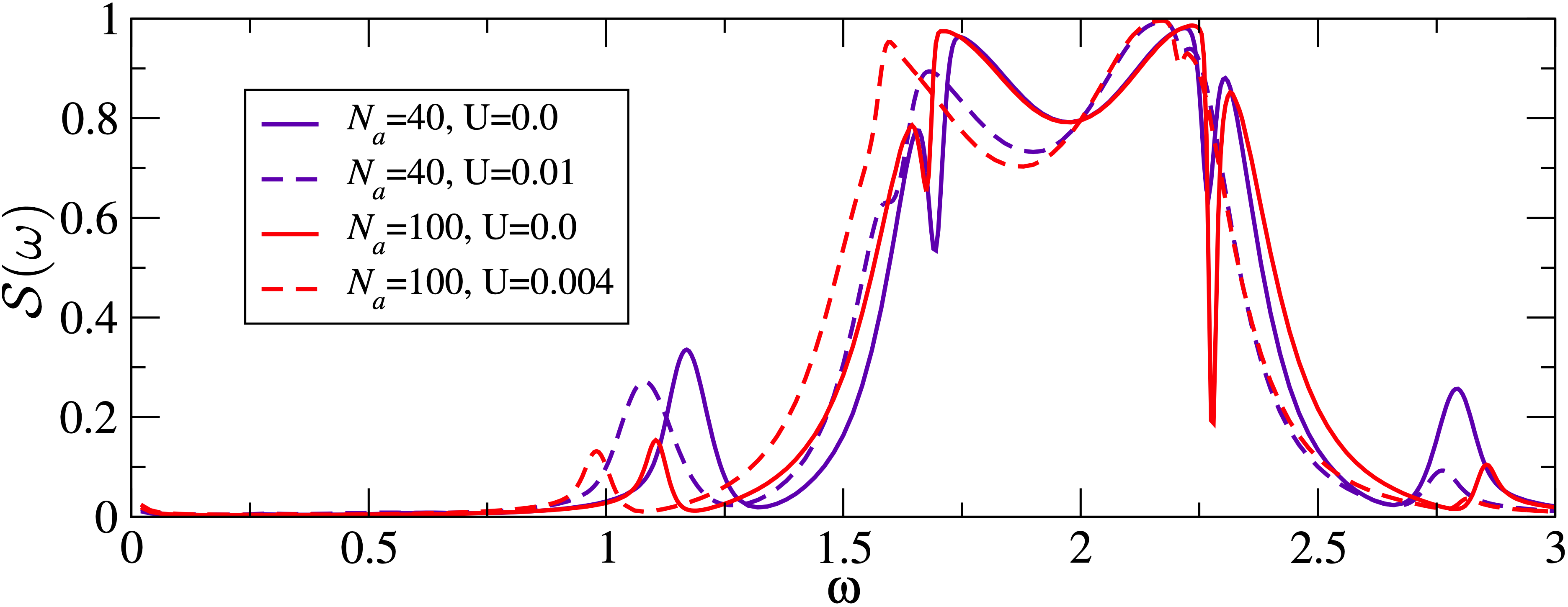
Figure 11: Resonance calculations with an initial coherent photon state with $\langle\hat{b}^{\dagger}\hat{b}\rangle=16$ and $\omega_{0}=2.0$. The parameters used are $U_{g}/N_{a}=U_{e}/N_{a}=U$ and $U_{eg}/N_{a}=U/2.0$, $g_{i}=0.3$, $g_{f}=0.1$, $\Gamma=0.02$, $E_{g}=0.0$ and $E_{e}=2.0$.

VII Conclusion

In this work, we have investigated the fluorescence of ultracold boson atoms in an optical cavity. By using an exact time-dependent configuration approach, we considered the case of (small) Bose-Hubbard lattices and of two-component Bose-Einstein condensates (2BEC). In the range of parameters explored, the fluorescent response from these systems is significantly affected by the strength of atom-atom interactions, the number of atoms in the system, and (for the finite-size optical lattices considered) the number of lattices sites.

For optical lattices, and at low interactions, the intensity of the SHG has a significant dependence on the number of atoms in the lattice, but is only marginally affected by interaction effects and system size (number of sites). The same occurs at large interactions, but only for a number of atoms smaller than the number of sites in the finite optical lattice. For a larger number of atoms, the intensity of the SHG peak gets reduced, due to an increased interaction penalty for having on average more than one-excited atom at each site. At large interactions, significant fluorescent spectral weight can also be found at very low frequencies: the spectrum of the many-atom system acquires a fine structure with several low-lying states which can be reached via optical excitation from the ground state.

A comparable scenario is found for resonant fluorescence, although the spectral intensity has now a non-monotonic dependence on the particle number (in relation to the number of lattice sites) at strong interactions. Furthermore, the Mollow sidebands (typical of resonant fluorescence) are noticeably hindered when photons are pumped in the cavity at a finite rate. We also observed that cavity leakage reduces the spectral intensity in Bose-Hubbard optical lattices and redshifts the SHG signal (in larger measure for strong atom-atom interactions).

Interesting indications also come from the case of a 2BEC: For SHG, and at low atom-cavity coupling, the spectra with different number of particles (and suitably rescaled interactions) are very similar; however, for a given particle number, interacting and non-interacting spectra are noticeably different. At large coupling, the SHG spectra significantly change on varying either the number of particles in the 2BEC, or the strength of the interactions. Furthermore, strong interactions redshift the SHG signal.

Conversely, at resonance, and for a given atom-cavity coupling, 2BEC spectra with different particle number are fairly similar to each other, irrespective of the strength of the atom-atom interactions (however, interacting spectra are redshifted compared to the non-interacting ones). In addition, the fluorescent spectra do not exhibit a Mollow triplet structure; rather, multiple peaks appear that coalesce in a nearly flat shape around the resonant frequency, a result possibly due to multi-photon effects and/or to the dressing by photons of the atomic levels.

As overall conclusive remark, our study identified some trends in the fluorescent response of ultracold bosons in a cavity, hopefully providing insight and motivation to further experimental and theoretical investigations of SHG in these systems. At the same time, due to the preliminary and incomplete nature of the present investigation, we foresee that additional features and physical scenarios will emerge from a more extensive parameter scan and/or extensions of the models and theoretical approaches employed here.

Figure 12: SHG for $U=0.0001$, $U_{eg}=U/2$ when $L=3$ and $L=4$. In all calculations $\eta=4.0$, $\omega_{0}=1.0$ and the initial state is $|\Phi_{0}^{SHG}\rangle$.

Appendix A Additional SHG results

Fig 12 displays the SHG results in the low interaction regime with $L=3$ and $L=4$. We observe that increasing the number of sites from $3$ to $4$ brings negligible effect to the fluorescent spectra. Furthermore, the results are very similar to those for $L=2$ in the main text. In Fig. 13 we consider the fluorescent response at resonant incident frequency $\omega_{0}=2.0$, for different interaction regimes, as determined by the value of $U$ ( $0\leq U\leq 5$, with $U_{eg}=U/2$ in all cases). The results shown are for a dimer ($L=2$) with $N_{a}=4$ atoms. The system is initially in the state $|\Phi_{0}^{Res}\rangle$, as specified in the main text. The incident pulse parameters are, $\tau_{1}=\tau_{2}=2.0$, $t_{1}=\frac{6\pi}{\omega_{0}}$, $t_{2}=\frac{31\pi}{\omega_{0}}$. The strength of the driving $g_{d}$ is chosen such that $\langle\hat{b}^{\dagger}\hat{b}\rangle\approx 16.0$ at the end of the drive. As observed for $N_{a}=3$ in the main text, the intensity of the spectrum decreases with increasing the interaction $U$.

Figure 13: Resonant fluorescent spectrum ($\omega_{0}=2$) in a dimer ($L=2$) with $N_{a}=4$ atoms, and its dependence on the atom-atom interaction strength $U$ (with $U_{g}=U/2$).

Appendix B Additional results at resonance

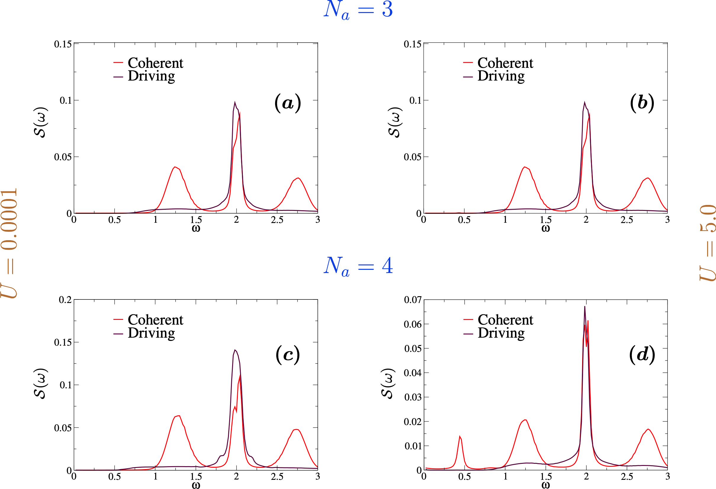
Figure 14: Resonance calculations ($\omega_{0}=2.0$) with $L=3$. In all panels, $U_{eg}=U/2$. The calculations with photon driving are with $\tau_{1}=\tau_{2}=2.0$, $t_{1}=\frac{6\pi}{\omega_{0}}$, $t_{2}=\frac{31\pi}{\omega_{0}}$, the initial state is $|\Phi_{0}^{Res}\rangle$ and the coupling $g_{d}$ is chosen such that $\langle\hat{b}^{\dagger}\hat{b}\rangle\approx 16$. For consistency, the calculation with the initial coherent state $\hat{b}|\eta\rangle=\eta|\eta\rangle$ are performed with $\eta=4$.

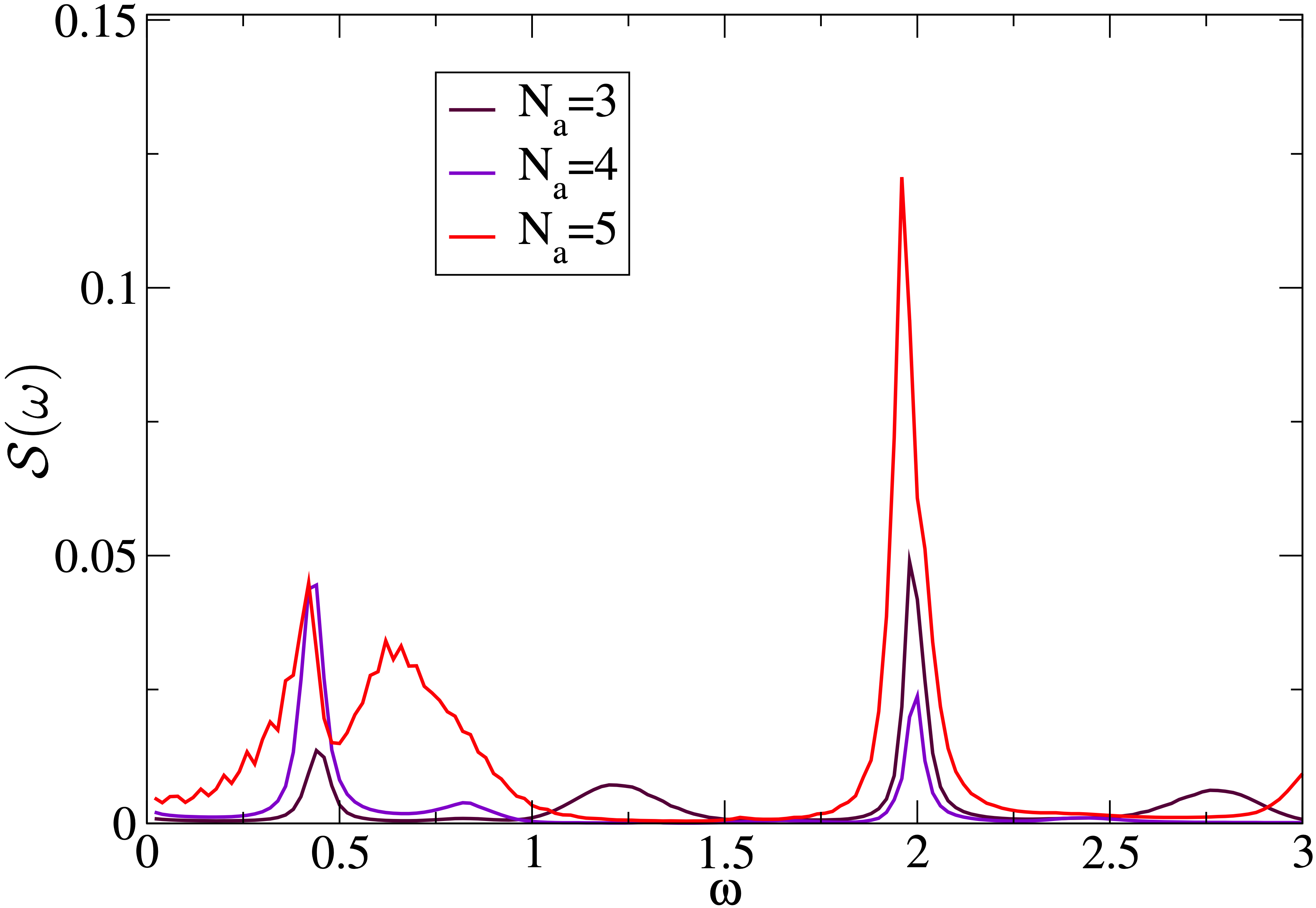
Figure 15: Results are of resonance calculations with $U=5.0$ and $U_{eg}=2.5$ (high interaction). In all calculations $L=2$, $\omega_{0}=2.0$ and $\eta=4$.

We here further illustrate the effect of laser driving at a finite rate. In Fig. 14, we compare fluorescence spectra obtained when starting from the cavity+system and pumping in time photons in the cavity, to results obtained when starting from the system’s ground state a coherent photon state. We clearly observe the Mollow sidebands in presence in the second case, and reduction of them in the presence of driving. The system considered is with $L=3$ and $N_{a}=3,4$; the other parameters are specified in the figure caption. A similar behavior is observed for other $L$ and $N_{a}$ values.

Starting from a coherent state, rather than pumping photons into the cavity with a driving laser, has also another effect: in Fig. 15, we display results at resonance for $L=2$ and $N_{a}=3,4,5$, and $U=5.0$ and $U_{eg}=U/2$, starting from a coherent state. In this case, the spectrum exhibits structures at lower frequencies, that are missing if we consider laser driving at a finite rate (which is the situation discussed in the main text).

References

- Zhai [2021] H. Zhai, Ultracold Atomic Physics (Cambridge University Press, 2021).
- Stwalley and Wang [1999] W. Stwalley and H. Wang, Special review lecture - photoassociation of ultracold atoms: A new spectroscopic technique, Journal of Molecular Spectroscopy 195, 194 (1999).
- Lewenstein et al. [2007] M. Lewenstein, A. Sanpera, V. Ahufinger, B. Damski, B. Sen(De), and U. Sen, Ultracold atomic gases in optical lattices: mimicking condensed matter physics and beyond, Advances in Physics 56, 243 (2007), https://doi.org/10.1080/00018730701223200 .
- Goldman et al. [2014] N. Goldman, G. Juzeliūnas, P. Öhberg, and I. B. Spielman, Light-induced gauge fields for ultracold atoms, Reports on Progress in Physics 77, 126401 (2014).
- Abanin et al. [2019] D. A. Abanin, E. Altman, I. Bloch, and M. Serbyn, Colloquium: Many-body localization, thermalization, and entanglement, Reviews of Modern Physics 91, 021001 (2019).
- Souza et al. [2023] R. S. Souza, A. Pelster, and F. E. dos Santos, Emergence of damped-localized excitations of the mott state due to disorder, New Journal of Physics 25, 10.1088/1367-2630/acdb92 (2023).
- Islam et al. [2015] R. Islam, R. Ma, P. M. Preiss, M. E. Tai, A. Lukin, M. Rispoli, and M. Greiner, Measuring entanglement entropy in a quantum many-body system, Nature 528, 77 (2015).
- Pezzè et al. [2018] L. Pezzè, A. Smerzi, M. K. Oberthaler, R. Schmied, and P. Treutlein, Quantum metrology with nonclassical states of atomic ensembles, Rev. Mod. Phys. 90, 035005 (2018).
- Pethick and Smith [2008] C. J. Pethick and H. Smith, Bose–Einstein Condensation in Dilute Gases, 2nd ed. (Cambridge University Press, 2008).
- Lewenstein et al. [2012] M. Lewenstein, A. Sanpera, and V. Ahufinger, Ultracold Atoms in Optical Lattices: Simulating quantum many-body systems (Oxford University Press, 2012).
- Anderson et al. [1995] M. Anderson, J. Ensher, M. Matthews, C. Wieman, and E. Cornell, Observation of Bose-Einstein condensation in a dilute atomic vapor, Science 269, 198 (1995).
- Davis et al. [1995] K. B. Davis, M. O. Mewes, M. R. Andrews, N. J. van Druten, D. S. Durfee, D. M. Kurn, and W. Ketterle, Bose-Einstein condensation in a gas of sodium atoms, Physical Review Letters 75, 3969 (1995).
- van Es et al. [2010] J. J. P. van Es, P. Wicke, A. H. van Amerongen, C. Rétif, S. Whitlock, and N. J. van Druten, Box traps on an atom chip for one-dimensional quantum gases, Journal of Physics B: Atomic, Molecular and Optical Physics 43, 155002 (2010).
- Al Khawaja and Stoof [2001] U. Al Khawaja and H. Stoof, Skyrmions in a ferromagnetic Bose-Einstein condensate, Nature 411, 918 (2001).
- Norcia et al. [2021] M. A. Norcia, C. Politi, L. Klaus, E. Poli, M. Sohmen, M. J. Mark, R. N. Bisset, L. Santos, and F. Ferlaino, Two-dimensional supersolidity in a dipolar quantum gas, Nature 596, 357 (2021).
- Eckel et al. [2018] S. Eckel, A. Kumar, T. Jacobson, I. B. Spielman, and G. K. Campbell, A rapidly expanding Bose-Einstein condensate: An expanding universe in the lab, Physical Review X 8, 021021 (2018).
- Hall et al. [1998] D. S. Hall, M. R. Matthews, J. R. Ensher, C. E. Wieman, and E. A. Cornell, Dynamics of component separation in a binary mixture of Bose-Einstein condensates, Physical Review Letters 81, 1539 (1998).
- Javanainen and Yoo [1996] J. Javanainen and S. M. Yoo, Quantum phase of a Bose-Einstein condensate with an arbitrary number of atoms, Physical Review Letters 76, 161 (1996).
- Milburn et al. [1997] G. J. Milburn, J. Corney, E. M. Wright, and D. F. Walls, Quantum dynamics of an atomic Bose-Einstein condensate in a double-well potential, Physical Review A 55, 4318 (1997).
- Dalton and Ghanbari [2012] B. J. Dalton and S. Ghanbari, Two mode theory of bose–einstein condensates: interferometry and the josephson model, Journal of Modern Optics 59, 287 (2012).
- Jaksch et al. [1998] D. Jaksch, C. Bruder, J. I. Cirac, C. W. Gardiner, and P. Zoller, Cold bosonic atoms in optical lattices, Physical Review Letters 81, 3108 (1998).
- Bloch [2005] I. Bloch, Ultracold quantum gases in optical lattices, Nature Physics 1, 23 (2005).
- Gross and Bloch [2017] C. Gross and I. Bloch, Quantum simulations with ultracold atoms in optical lattices, Science 357, 995 (2017), https://www.science.org/doi/pdf/10.1126/science.aal3837 .
- Schäfer et al. [2020] F. Schäfer, T. Fukuhara, S. Sugawa, Y. Takasu, and Y. Takahashi, Tools for quantum simulation with ultracold atoms in optical lattices, Nature Reviews Physics 2, 411 (2020).
- Batrouni et al. [2002] G. G. Batrouni, V. Rousseau, R. T. Scalettar, M. Rigol, A. Muramatsu, P. J. H. Denteneer, and M. Troyer, Mott domains of bosons confined on optical lattices, Physical Review Letters 89, 117203 (2002).
- Fromhold et al. [2000] T. M. Fromhold, C. R. Tench, S. Bujkiewicz, P. B. Wilkinson, and F. W. Sheard, Quantum chaos for cold atoms in an optical lattice with a tilted harmonic trap, Journal of Optics B: Quantum and Semiclassical Optics 2, 628 (2000).
- Pichler et al. [2016] H. Pichler, G. Zhu, A. Seif, P. Zoller, and M. Hafezi, Measurement protocol for the entanglement spectrum of cold atoms, Physical Review X 6, 041033 (2016).
- Galitski et al. [2019] V. Galitski, G. Juzeliūnas, and I. B. Spielman, Artificial gauge fields with ultracold atoms, Physics Today 72, 38 (2019), https://pubs.aip.org/physicstoday/article-pdf/72/1/38/10121390/38_1_online.pdf .
- Takamoto et al. [2005] M. Takamoto, F.-L. Hong, R. Higashi, and H. Katori, An optical lattice clock, Nature 435, 321 (2005).
- Borkowski [2018] M. Borkowski, Optical lattice clocks with weakly bound molecules, Physical Review Letters 120, 083202 (2018).
- Zoubi and Ritsch [2009] H. Zoubi and H. Ritsch, Quantum phases of bosonic atoms with two levels coupled by a cavity field in an optical lattice, Physical Review A 80, 053608 (2009).
- Peyronel et al. [2012] T. Peyronel, O. Firstenberg, Q.-Y. Liang, S. Hofferberth, A. V. Gorshkov, T. Pohl, M. D. Lukin, and V. Vuletić, Quantum nonlinear optics with single photons enabled by strongly interacting atoms, Nature 488, 57 (2012).
- Ritsch et al. [2013] H. Ritsch, P. Domokos, F. Brennecke, and T. Esslinger, Cold atoms in cavity-generated dynamical optical potentials, Rev. Mod. Phys. 85, 553 (2013).
- Schleich [2001] W. P. Schleich, Quantum Optics in Phase Space (Wiley-VCH, Berlin, 2001).
- Farokh Mivehvar and Ritsch [2021] T. D. Farokh Mivehvar, Francesco Piazza and H. Ritsch, Cavity qed with quantum gases: new paradigms in many-body physics, Advances in Physics 70, 1 (2021), https://doi.org/10.1080/00018732.2021.1969727 .
- Ghasemian and Tavassoly [2017] E. Ghasemian and M. K. Tavassoly, Quantum dynamics of a BEC interacting with a single-mode quantized field under the influence of a dissipation process: thermal and squeezed vacuum reservoirs, Laser Physics 27, 095202 (2017).
- Ghasemian and Tavassoly [2018] E. Ghasemian and M. K. Tavassoly, Spontaneous emission originating from atomic BEC interacting with a single-mode quantized field, Communications in Theoretical Physics 69, 711 (2018).
- Ghasemian and Tavassoly [2021] E. Ghasemian and M. Tavassoly, Dynamics of an atomic Bose–Einstein condensate interacting with nonlinear quantized field under the influence of Stark effect, Physica A: Statistical Mechanics and its Applications 562, 125323 (2021).
- Kumar et al. [2011] T. Kumar, A. B. Bhattacherjee, and ManMohan, Two-photon nonlinear spectroscopy of periodically trapped ultracold atoms in a cavity, International Journal of Modern Physics B 25, 1737 (2011).
- Maschler and Ritsch [2005] C. Maschler and H. Ritsch, Cold atom dynamics in a quantum optical lattice potential, Physical Review Letters 95, 260401 (2005).
- Bloembergen [1982] N. Bloembergen, Nonlinear optics and spectroscopy, Rev. Mod. Phys. 54, 685 (1982).
- Ciappina et al. [2017] M. F. Ciappina, J. A. Pérez-Hernández, A. S. Landsman, W. A. Okell, S. Zherebtsov, B. Förg, J. Schötz, L. Seiffert, T. Fennel, T. Shaaran, T. Zimmermann, A. Chacón, R. Guichard, A. Zaïr, J. W. G. Tisch, J. P. Marangos, T. Witting, A. Braun, S. A. Maier, L. Roso, M. Krüger, P. Hommelhoff, M. F. Kling, F. Krausz, and M. Lewenstein, Attosecond physics at the nanoscale, Reports on Progress in Physics 80, 054401 (2017).
- Fu and Cui [2019] X. Fu and T. J. Cui, Recent progress on metamaterials: From effective medium model to real-time information processing system, Progress in Quantum Electronics 67, 100223 (2019).
- Andraud and Maury [2009] C. Andraud and O. Maury, Lanthanide complexes for nonlinear optics: From fundamental aspects to applications, European Journal of Inorganic Chemistry 2009, 4357 (2009).
- Yue et al. [2011] S. Yue, M. Slipchenko, and J.-X. Cheng, Multimodal nonlinear optical microscopy, Laser & Photonics Reviews 5, 496 (2011).
- Combes et al. [2021] G. F. Combes, A.-M. Vučković, M. Perić Bakulić, R. Antoine, V. Bonačić-Koutecky, and K. Trajković, Nanotechnology in tumor biomarker detection: The potential of liganded nanoclusters as nonlinear optical contrast agents for molecular diagnostics of cancer, Cancers 13, 10.3390/cancers13164206 (2021).
- Chen et al. [2021] J. Chen, C.-L. Hu, F. Kong, and J.-G. Mao, High-performance second-harmonic-generation (shg) materials: New developments and new strategies, Accounts of Chemical Research 54, 2775 (2021).
- Cini et al. [1993] M. Cini, A. D’Andrea, and C. Verdozzi, Many-photon effects in inelastic light-scattering, Physics Letters A 180, 430 (1993).
- Cini et al. [1995] M. Cini, A. D’Andrea, and C. Verdozzi, Many-photon effects in inelastic light-scattering - theory and model applications, International Journal of Modern Physics B 9, 1185 (1995).
- Landig et al. [2016] R. Landig, L. Hruby, N. Dogra, M. Landini, R. Mottl, T. Donner, and T. Esslinger, Quantum phases from competing short- and long-range interactions in an optical lattice, Nature 532, 476 (2016).
- Nagy et al. [2018] D. Nagy, G. Kónya, P. Domokos, and G. Szirmai, Quantum noise in a transversely-pumped-cavity bose-hubbard model, Physical Review A 97, 063602 (2018).
- Zoubi and Ritsch [2007] H. Zoubi and H. Ritsch, Excitons and cavity polaritons for ultracold atoms in an optical lattice, Physical Review A 76, 013817 (2007).
- Maschler et al. [2008] C. Maschler, I. B. Mekhov, and H. Ritsch, Ultracold atoms in optical lattices generated by quantized light fields, The European Physical Journal D 46, 545 (2008).
- Zoubi and Ritsch [2013] H. Zoubi and H. Ritsch, Chapter 3 - Excitons and cavity polaritons for optical lattice ultracold atoms, in Advances In Atomic, Molecular, and Optical Physics, Vol. 62, edited by E. Arimondo, P. R. Berman, and C. C. Lin (Academic Press, 2013) pp. 171–229.
- Cohen-Tannoudji [1996] C. N. Cohen-Tannoudji, The Autler-Townes effect revisited, in Amazing Light: A Volume Dedicated To Charles Hard Townes On His 80th Birthday, edited by R. Y. Chiao (Springer New York, New York, NY, 1996) pp. 109–123.
- Hargart et al. [2016] F. Hargart, K. Roy-Choudhury, T. John, S. L. Portalupi, C. Schneider, S. Höfling, M. Kamp, S. Hughes, and P. Michler, Probing different regimes of strong field light–matter interaction with semiconductor quantum dots and few cavity photons, New Journal of Physics 18, 123031 (2016).
- Viñas Boström et al. [2020] E. Viñas Boström, A. D’Andrea, M. Cini, and C. Verdozzi, Time-resolved multiphoton effects in the fluorescence spectra of two-level systems at rest and in motion, Physical Review A 102, 013719 (2020).
- Gopalakrishna et al. [2023] M. Gopalakrishna, E. Viñas Boström, and C. Verdozzi, Photon pumping, photodissociation and dissipation at interplay for the fluorescence of a molecule in a cavity, SciPost Phys. 15, 138 (2023).
- Caldeira and Leggett [1983] A. O. Caldeira and A. J. Leggett, Quantum tunnelling in a dissipative system, Annals of Physics 149, 374 (1983).
- Venkataraman et al. [2013] V. Venkataraman, A. D. K. Plato, T. Tufarelli, and M. S. Kim, Affecting non-markovian behaviour by changing bath structures, Journal of Physics B: Atomic, Molecular and Optical Physics 47, 015501 (2013).
- Horsfield et al. [2004] A. P. Horsfield, D. R. Bowler, A. J. Fisher, T. N. Todorov, and M. J. Montgomery, Power dissipation in nanoscale conductors: classical, semi-classical and quantum dynamics, Journal of Physics: Condensed Matter 16, 3609 (2004).
- Stahl and Potthoff [2017] C. Stahl and M. Potthoff, Anomalous spin precession under a geometrical torque, Physical Review Letters 119, 227203 (2017).
- Bai et al. [2022] H. Bai, L. Han, X. Y. Feng, Y. J. Zhou, R. X. Su, Q. Wang, L. Y. Liao, W. X. Zhu, X. Z. Chen, F. Pan, X. L. Fan, and C. Song, Observation of spin splitting torque in a collinear antiferromagnet , Physical Review Letters 128, 197202 (2022).
- Gay-Balmaz and Tronci [2023] F. Gay-Balmaz and C. Tronci, Dynamics of mixed quantum–classical spin systems, Journal of Physics A: Mathematical and Theoretical 56, 144002 (2023).
- Andrade et al. [2009] X. Andrade, A. Castro, D. Zueco, J. L. Alonso, P. Echenique, F. Falceto, and A. Rubio, Modified Ehrenfest formalism for efficient large-scale ab initio molecular dynamics, Journal of Chemical Theory and Computation 5, 728 (2009).
- [66] A direct way to go beyond finite Bose-Hubbard systems would be to consider an optical lattice described by the Bose Hubbard model at large and, for example, to focus on the ideal/non ideal superfluid phase in the presence of quantum light modes. This is a rather interesting problem, which however requires additional developments; work in along these lines is currently in process.
- Kuang and Zhou [2003] L.-M. Kuang and L. Zhou, Generation of atom-photon entangled states in atomic Bose-Einstein condensate via electromagnetically induced transparency, Physical Review A 68, 043606 (2003).
- Huang et al. [2008] C. Huang, J. Fang, H. He, F. Kong, and M. Zhou, Squeezing of an atom laser originating from atomic Bose-Einstein condensate interacting with light field, Physica A: Statistical Mechanics and its Applications 387, 3449 (2008).
- Dicke [1954] R. H. Dicke, Coherence in spontaneous radiation processes, Phys. Rev. 93, 99 (1954).
- Kirton et al. [2019] P. Kirton, M. M. Roses, J. Keeling, and E. G. Dalla Torre, Introduction to the dicke model: From equilibrium to nonequilibrium, and vice versa, Advanced Quantum Technologies 2, 1800043 (2019).
- Nagy et al. [2010] D. Nagy, G. Kónya, G. Szirmai, and P. Domokos, Dicke-model phase transition in the quantum motion of a Bose-Einstein condensate in an optical cavity, Physical Review Letters 104, 130401 (2010).