The Magellan M2FS spectroscopic survey of high-redshift galaxies: the brightest Lyman-break galaxies at
Abstract
We present a study of a sample of 45 spectroscopically confirmed, UV luminous galaxies at . They were selected as bright Lyman-break galaxies (LBGs) using deep multi-band optical images in more than 2 deg2 of the sky, and subsequently identified via their strong Lyemission. The majority of these LBGs span an absolute UV magnitude range from to mag with Lyequivalent width (EW) between 10 and 200 Å, representing the most luminous galaxies at in terms of both UV continuum emission and Lyline emission. We model the SEDs of 10 LBGs that have deep infrared observations from HST, JWST, and/or Spitzer, and find that they have a wide range of stellar masses and ages. They also have high star-formation rates ranging from a few tens to a few hundreds of Solar mass per year. Five of the LBGs have JWST or HST images and four of them show compact morphology in these images, including one that is roughly consistent with a point source, suggesting that UV luminous galaxies at this redshift are generally compact. The fraction of our photometrically selected LBGs with strong Lyemission ( Å) is about , which is consistent with previous results and supports a moderate evolution of the IGM opacity at the end of cosmic reionization. Using deep X-ray images, we do not find evidence of strong AGN activity in these galaxies, but our constraint is loose and we are not able to rule out the possibility of any weak AGN activity.
1 Introduction
High-redshift () galaxies are a key probe to understand the early Universe, including the early galaxy formation and evolution, the development of large-scale structures, and the history of cosmic reionization. In the past twenty years, a number of works have been conducted to search for high-redshift galaxies, and the number of known galaxies has increased dramatically thanks to the advances of instrumentation on the Hubble Space Telescope (HST) and large ground-based telescopes (e.g., Kashikawa et al. 2006; Vanzella et al. 2009; Hu et al. 2010; Wilkins et al. 2010; Stark et al. 2011; McLeod et al. 2016; Bouwens et al. 2021; Zheng et al. 2017; Ono et al. 2018; Ning et al. 2020; Wold et al. 2022). The majority of the earlier known galaxies at are photometrically selected Lyman-break galaxies (LBGs) or LBG candidates selected by the dropout technique. The narrowband technique (or the Lytechnique) is a complementary method to find high-redshift galaxies. Ground-based narrowband imaging surveys are efficient in finding Lyemitting galaxies (Lyemitters, or LAEs) at certain redshift slices such as , 6.6, and 7.0 that correspond to wavelength windows with weak OH sky lines.
Before the launch of James Webb Space Telescope (JWST), the majority of the photometrically selected high-redshift galaxies have not been spectroscopically observed. While narrowband selected LAE candidates typically have a high success rate of spectroscopic confirmation, only a small fraction of photometrically selected LBGs are spectroscopically confirmed (e.g., Toshikawa et al. 2012; Finkelstein et al. 2013; Watson et al. 2015; Roberts-Borsani et al. 2016; Song et al. 2016; Larson et al. 2022). Spectroscopic observations are important to understand LBGs, because they can not only tell us whether an object is a real LBG, but also provide a key parameter, redshift. Large samples of high-redshift galaxies have been frequently used to measure galaxy properties, such as UV slopes (e.g., Dunlop et al. 2012; Finkelstein et al. 2012a; Bouwens et al. 2014), galaxy morphology (e.g., Guaita et al. 2015; Kawamata et al. 2015; Shibuya et al. 2015, 2016; Curtis-Lake et al. 2016; Kobayashi et al. 2016; Liu et al. 2017; Naidu et al. 2022), stellar populations, and star-formation rates (e.g., Egami et al. 2005; Stark et al. 2013; González et al. 2014; Faisst et al. 2016; Castellano et al. 2017; Karman et al. 2017). These studies are mostly based on photometric samples.
Recently, JWST is revolutionizing our understanding of high-redshift galaxies. JWST is not only breaking redshift records for the most distant objects (e.g., Arrabal Haro et al., 2023; Curtis-Lake et al., 2023; Fujimoto et al., 2023; Hsiao et al., 2023; Roberts-Borsani et al., 2023), but also rapidly expanding the sample sizes of high-redshift galaxies, photometrically and spectroscopically (e.g., Atek et al. 2023; Champagne et al. 2023; Leethochawalit et al. 2023; Yan et al. 2023). In particular, JWST NIRCam and NIRISS observations offer slitless spectroscopy that makes it feasible to obtain spectra for large galaxy samples (e.g., Matthee et al. 2023; Oesch et al. 2023; Wang et al. 2023). In addition, JWST NIRSpec grating observations provide medium-resolution spectra that allow detailed studies of line emission and absorption (e.g., Bunker et al. 2023; Mascia et al. 2023; Prieto-Lyon et al. 2023; Tang et al. 2023; Tacchella et al. 2023). Despite the great power of JWST, its field-of-view is small compared to ground-based telescopes. Therefore, large-area, ground-based observations are highly complementary to JWST observations.
High-redshift galaxies are also thought to be the major source of ionizing photons at the epoch of cosmic reionization. Recent studies have suggested that star-forming galaxies, rather than quasars or AGN, provide most of the ionizing photons needed for reionization (e.g., Finkelstein et al. 2012b; Robertson et al. 2015; Onoue et al. 2017; Jiang et al. 2022). Spectroscopic samples of high-redshift LBGs can be used to constrain the properties of the IGM during this epoch. For example, Lyphotons are easily absorbed by neutral hydrogen, making the Lyline a sensitive probe of the ionization state of the IGM. Therefore, the fraction of LBGs that exhibit strong Lyemission lines can trace the fraction of neutral hydrogen in the IGM at . This so-called Lyvisibility test from previous works has shown that the fraction of LBGs with strong Lyemission increases steadily from to 6 and then declines sharply towards (e.g., Stark et al. 2010, 2011; Ono et al. 2012; Schenker et al. 2012; Finkelstein et al. 2013; Tilvi et al. 2014; Vanzella et al. 2014; Cassata et al. 2015; Schmidt et al. 2016; Jung et al. 2018, 2022). This is broadly consistent with the evolving neutral fraction in the IGM at the end of the reionization epoch.
In this paper, we present a sample of 45 LBGs with spectroscopically confirmed Lyemission lines at from a survey of high-redshift galaxies using the Magellan telescope (Jiang et al., 2017). In Section 2, we introduce the survey program, target selection, spectroscopic observations, and data reduction. In Section 3, we construct our spectroscopic sample of LBGs. In Section 4, we present the properties of the galaxies using spectra and images from multi-wavelength observations. We discuss our results in Section 5, and summarize our paper in Section 6. Throughout the paper, we use a standard flat cosmology with , and . All magnitudes refer to the AB system.
2 Target Selection and Spectroscopic Observations
2.1 A Magellan M2FS Survey of Galaxies
| Fields | Coordinates | Area | Filters | Candidates | Good | Possible | |||
|---|---|---|---|---|---|---|---|---|---|
| (J2000) | (deg2) | (mag) | (mag) | (mag) | |||||
| SXDS | 02:18:00–05:00:00 | ||||||||
| A370a | 02:39:55–01:35:24 | ||||||||
| ECDFS | 03:32:25–27:48:18 | ||||||||
| COSMOS | 10:00:29+02:12:21 |
Note. — Col.(1): Field names. Col.(2): Center coordinates. Col.(3): Area coverage. Col.(4): Broadband filters. Col.(5-7): Magnitude limits ( detections in a -diameter aperture). Col.(8): Numbers of LBG candidates. Col.(9-10): Numbers of spectroscopically confirmed LBGs in the ‘good’ sample and the ‘possible’ sample.
We carried out a large spectroscopic survey of galaxies at , using the large field-of-view (FoV), fiber-fed, multi-object spectrograph M2FS (Mateo et al., 2012) on the 6.5 m Magellan Clay telescope. The overview of the survey program was provided in Jiang et al. (2017). The survey was designed to build a large and homogeneous sample of high-redshift galaxies, including LAEs at and 6.6, and LBGs with strong Lyemission at . Based on this sample, we can study the properties of these galaxies, the Lyluminosity function (LF) and its evolution at high redshift, high-redshift protoclusters, cosmic reionization, etc. Taking advantage of a -diameter FoV, M2FS is very efficient in identifying relatively bright high-redshift galaxies (e.g., Oyarzún et al. 2016, 2017). The fields that we chose to observe are well-studied deep fields, including the Subaru XMM-Newton Deep Survey (SXDS), A370, the Extended Chandra Deep Field- South (ECDFS), COSMOS, etc. They cover a total of deg2. These fields have deep Subaru Suprime-Cam imaging data in a series of broad bands and narrow bands (e.g., NB816 and NB921). The images have been used to select LAEs at and 6.6 and LBGs at in the survey program. The fields are summarized in Table 1. Some of the fields were later observed by Subaru Hyper Suprime-Cam (HSC) (Aihara et al., 2022), but we did not use the HSC data by the time of our observations.
The M2FS observations of the program have been completed and the data have been reduced. From the survey, Ning et al. (2020) built a large sample of 260 LAEs at and Jiang et al. (2018) discovered a giant protocluster at . Ning et al. (2022) then assembled a sample of 36 LAEs at . By comparing with the LyLF, they confirmed that there is a rapid LF evolution at the faint end, but there is a lack of evolution at the bright end. Wu et al. (2020) detected diffuse Lyhalos around galaxies at by stacking 310 spectroscopically confirmed LAEs. In this paper, we focus on luminous LBGs at . The details of the target selection is presented in Section 2.3.
2.2 Spectroscopic Observations and Data Reduction
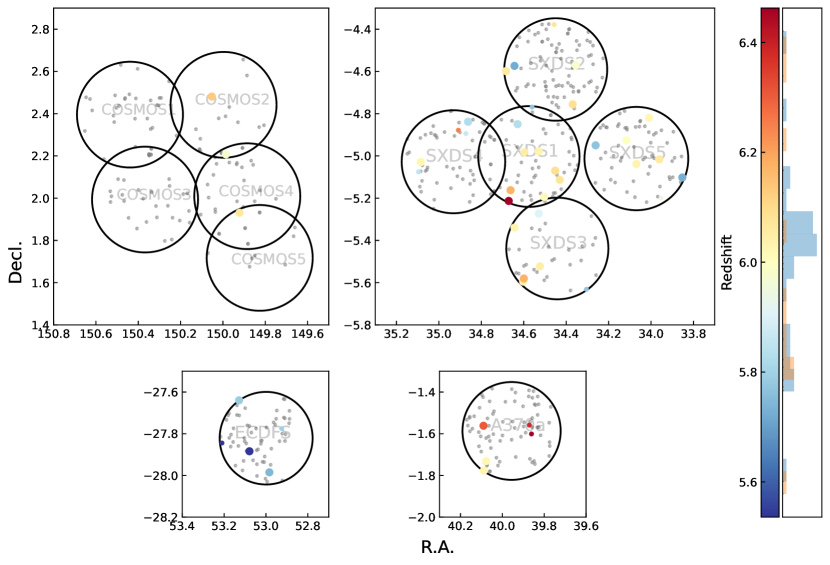
We carried out the M2FS observations in 2015–2018. The resolving power of the spectra is , and the wavelength coverage is roughly from 7600 to 9600 Å, corresponding to a redshift range of for the detection of the Lyemission line. The selection of M2FS pointing centers was limited by the number and spatial distribution of bright stars that were used for guiding, alignment, and primary-mirror wavefront corrections. The layout of the pointings is shown in Figure 1. The effective integration time per pointing was about 5 hr on average, and the individual exposure time was 30 min, 45 min, or 1 hr, depending on airmass and weather conditions.
We used our own customized pipeline for data reduction, including bias (overscan) correction, dark subtraction, flat-fielding, cosmic ray identification, wavelength calibration, and sky subtraction. For detailed steps, see Jiang et al. (2017). The pipeline produces combined 1D and 2D spectra as well as the 2D spectra of individual exposures. This pipeline is performed for all targets in the same fields, including the candidates of LAEs and LBGs. The final 1D and 2D spectra were used to identify Lyemission lines.
2.3 Selection of LBG Candidates
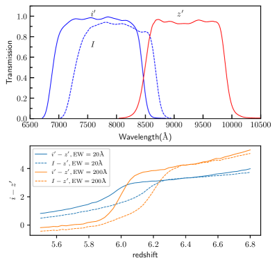
Our M2FS observations included a sample of luminous LBG candidates at . Deep Subaru Suprime-Cam images were used for the selection of these candidates. The selection was mainly based on the color (here means either or ). The upper panel of Figure 2 shows the filters that were used for our target selection. The selection limit is detections in the band. We applied the following color cuts,
To illustrate the evolution of the color with redshift, we produced a simple galaxy spectrum consisting of a power-law continuum and a Lyemission line. The power-law continuum has a fixed slope of –2.0, and the Lyequivalent width (EW) has two values, 20 and 200 Å, respectively. We then apply the Inoue et al. (2014) IGM attenuation models to the spectra. The result is shown in the lower panel of Figure 2. The value of increases rapidly at . With our selection criteria, galaxies with can be selected. The actual selection function is more complex and depends on the galaxy continuum emission and Lyline emission. We also required no detections () in any bands bluer than (or ), assuming that no flux can be detected at the wavelength bluer than the Lyman limit. Each candidate was visually inspected.
Compared to the previous selection criteria of LBGs (e.g., Ono et al. 2018; Bouwens et al. 2021), our selection criteria are relatively conservative. Previous studies usually applied redder colors (e.g., in Ono et al. 2018), and often considered infrared photometry. For example, many contaminants of high-redshift galaxies are late-type dwarf stars or low-redshift red (dusty) galaxies, and thus tend to have redder colors in the near-IR. We did not use near-IR data, despite the fact that some of our fields are covered by deep near-IR images. Our conservative criteria allow us to include less promising candidates and thus achieve higher sample completeness. On the other hand, it means a relatively lower efficiency, i.e., a larger fraction of contaminants. It is not a concern in our program, since we have enough fibers to cover almost all these candidates. In Table 1, Column 8 shows the numbers of the candidates in each field that were observed by our program.
3 Spectroscopic Results
3.1 LyLine Identification and a Sample of LBGs
In this subsection, we will describe how to identify Lyemission lines in the spectra, and present two samples of spectroscopically confirmed LBGs, including a ‘good’ sample with high confidence and a ‘possible’ sample with lower confidence. We will then derive some basic properties of the Lylines.
We use both 1D and 2D spectra to identify Lyemission lines. We first carry out an initial search. For each galaxy, we bin its 1D spectrum by 3 Å and search for an emission line with signal-to-noise ratio S/N in the whole wavelength range. For a line in the ‘good’ sample, it needs to cover at least 5 contiguous pixels with S/N in each pixel in the binned spectrum. This is determined by the typical Lyemission line width in our spectra. For the ‘possible’ sample, we allow a line to cover only 3 or 4 contiguous pixels with S/N . The S/N of a line is estimated by summing up the corresponding pixels of the line in the original spectrum. The reason of adopting a criterion of S/N is that most of the regions in the LBG spectra are contaminated by strong OH sky lines. If a Lyline is close to OH lines, it could be severely affected by sky line residuals after the sky background subtraction.
After the initial screening above, we visually inspect each identified emission line in the 2D spectra, including the combined spectrum and the spectra of individual exposures. Obvious false detections are removed. The Lyemission line of a galaxy is often much broader than other emission lines at much lower redshift in the observed frame due to the (1+) broadening. It also shows an asymmetric profile due to strong IGM absorption and ISM kinematics. Possible contaminant lines from low-redshift galaxies usually appear narrow and symmetric, including H, O III 5007, or H emission lines. In addition, our resolving power of can nearly resolve the O II 3727, 3729 doublet. To quantify the asymmetry of the Lyline, we calculate the weighted skewness introduced by Shimasaku et al. (2006). This is the skewness (or third moment) of the line multiplied by , where and are the wavelengths where the flux drops to of its peak value at the red and blue sides of the line, respectively. Since the Lyemission of high-redshift galaxies tends to be broader than other emission lines of lower-redshift galaxies, this line width factor enhances the difference between Lyand other lines. The Ly values of the LBGs in our ‘good’ sample and ‘possible’ sample range from 2.3 to 18.4 and from 2.1 to 12.2, respectively. In comparison, we also calculate of 10 emission lines that are identified as low-redshift interlopers based on their double-peak (e.g., an O II 3727, 3729 doublet at ), or based on the detection of other lines at the same redshift in the spectra (e.g., an O III 5007 and corresponding O III 4959 at ). Their values span a range from to . Usually has been used as a threshold to distinguish Lyfrom other lines, but the asymmetric shape of a high-redshift Lyemission line may not be obvious when its S/N is relatively low (e.g., Ning et al., 2022). For three LBGs with , they were not detected in two blue bands and , so we put them in the ‘possible’ sample.
We emphasize that in our LBG candidate selection procedure addressed in Section 2.3, we required non-detections for the candidates in the - and -band images. These images reach a great depth of mag. They can efficiently exclude low-redshift interlopers.
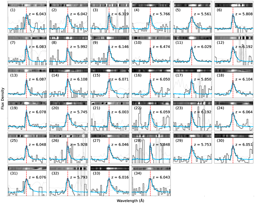
Finally, the ‘good’ sample of 34 LBGs has convincing, luminous Lyemission lines with S/N and asymmetric profiles. Figure 3 shows the 1D and 2D spectra in the Lyregion of the 36 LBGs in the ‘good’ sample. We can see that strong emission lines clearly show asymmetric line shapes due to the IGM absorption and ISM kinematics. The ‘possible’ sample contains 11 LBGs with less promising Lyemission lines. We show all the confirmed LBGs in Table 2. Column 5 lists the spectroscopic redshifts measured from the Lylines, and their errors are smaller than 0.001. Figure 1 illustrates the positions of the targets in the five fields, including the observed candidates (all points) and the spectroscopically confirmed LBGs (color-coded points). The large circles represent the M2FS pointings. Despite the fact that the exposure time and depth of the individual pointings are similar, the numbers of the confirmed LBGs in these pointings are quite different, suggesting the existence of significant cosmic variance. As mentioned in Ning et al. (2020, 2022), COSMOS1 and COSMOS3 have some alignment problems during the observations, so they only have a few LBGs confirmed.
3.2 Properties of the LyEmission Lines
We measure redshifts and Lyline flux for the LBGs using a Lyprofile template. The template is a composite Lyspectrum of a large number of LAEs at (Ning et al., 2020). For each LBG, we first estimate an initial redshift using the wavelength of the Lyline peak (1215.67 Å). We then refine this redshift and model the Lyprofile as follows. From the Lytemplate, we generate a set of model spectra for a grid of peak values, line widths, and redshifts. The peak values vary from 0.9 to 1.1 (times of the observed peak value) with a step size of 0.01. The line widths are from 0.5 to 2.0 times the original width with a step size of 0.1. The redshift values vary within the initial redshift with a step size of 0.0001. We find the best-fit model for each LBG using the method. The best-fit redshifts are listed in Column 5 of Table 2.
| No. | Field | R.A. | Decl. | Redshift | log10L(Ly) | LyEW | ||||
|---|---|---|---|---|---|---|---|---|---|---|
| (J2000) | (J2000) | (mag) | (mag) | (erg/s) | (mag) | (Å) | ||||
| Good Sample | ||||||||||
| A370a | 02:40:21.24 | –01:46:37.52 | ||||||||
| A370a | 02:40:18.51 | –01:43:51.66 | ||||||||
| A370a | 02:40:21.60 | –01:33:42.16 | ||||||||
| ECDFS | 03:31:56.08 | –27:59:06.50 | ||||||||
| ECDFS | 03:32:18.92 | –27:53:02.81 | ||||||||
| ECDFS | 03:32:30.85 | –27:38:22.20 | ||||||||
| COSMOS | 09:59:41.18 | +01:55:51.75 | ||||||||
| COSMOS | 09:59:56.54 | +02:12:27.15 | ||||||||
| COSMOS | 10:00:12.59 | +02:28:52.08 | ||||||||
| SXDS1 | 02:18:41.01 | –05:12:47.18 | ||||||||
| SXDS1 | 02:18:00.91 | –05:11:37.77 | ||||||||
| SXDS1 | 02:18:38.92 | –05:09:44.02 | ||||||||
| SXDS1 | 02:17:43.25 | –05:06:47.60 | ||||||||
| SXDS1 | 02:17:48.40 | –05:04:10.79 | ||||||||
| SXDS1 | 02:18:23.34 | –04:58:58.18 | ||||||||
| SXDS1 | 02:18:07.14 | –04:58:41.50 | ||||||||
| SXDS1 | 02:18:30.93 | –04:50:58.73 | ||||||||
| SXDS2 | 02:17:28.71 | –04:45:19.61 | ||||||||
| SXDS2 | 02:18:44.06 | –04:35:54.24 | ||||||||
| SXDS2 | 02:18:34.48 | –04:34:25.86 | ||||||||
| SXDS2 | 02:17:25.27 | –04:34:12.85 | ||||||||
| SXDS3 | 02:18:24.72 | –05:35:41.82 | ||||||||
| SXDS3 | 02:18:23.90 | –05:34:49.34 | ||||||||
| SXDS3 | 02:18:05.68 | –05:31:21.90 | ||||||||
| SXDS3 | 02:18:34.47 | –05:20:20.96 | ||||||||
| SXDS3 | 02:18:06.96 | –05:16:21.93 | ||||||||
| SXDS4 | 02:20:20.49 | –05:01:45.06 | ||||||||
| SXDS4 | 02:19:26.97 | –04:50:17.71 | ||||||||
| SXDS5 | 02:15:24.62 | –05:06:07.27 | ||||||||
| SXDS5 | 02:16:16.53 | –05:02:17.80 | ||||||||
| SXDS5 | 02:15:50.69 | –05:00:57.88 | ||||||||
| SXDS5 | 02:17:02.70 | –04:56:59.28 | ||||||||
| SXDS5 | 02:16:27.81 | –04:55:34.25 | ||||||||
| SXDS5 | 02:16:02.36 | –04:49:08.81 | ||||||||
| Possible Sample | ||||||||||
| A370a | 02:39:26.57 | –01:36:03.84 | ||||||||
| A370a | 02:39:28.99 | –01:33:31.00 | ||||||||
| ECDFS | 03:32:50.43 | –27:50:40.23 | ||||||||
| ECDFS | 03:31:41.99 | –27:46:30.91 | ||||||||
| SXDS2 | 02:18:14.62 | –04:46:07.52 | ||||||||
| SXDS2 | 02:17:49.61 | –04:22:41.36 | ||||||||
| SXDS3 | 02:17:13.11 | –05:37:53.43 | ||||||||
| SXDS4 | 02:20:22.93 | –05:04:31.83 | ||||||||
| SXDS4 | 02:19:29.35 | –04:53:38.27 | ||||||||
| SXDS4 | 02:19:37.99 | –04:52:41.57 | ||||||||
| SXDS5 | 02:15:48.66 | –05:11:58.28 | ||||||||
Note. — Col.(1): Object numbers. Col.(2): Field names. Col.(3-4): Source coordinates. Col.(5): Spectroscopic redshifts (their errors are smaller than 0.001). Col.(6-7): Subaru Suprime-Cam band and band magnitudes. The upper limits indicate detections. Col.(8): Lyline luminosities. Col.(9): Absolute UV magnitudes at rest-frame 1500 Å. Col.(10): Lyline EWs. Col.(11): UV slopes calculated from multi-band data.
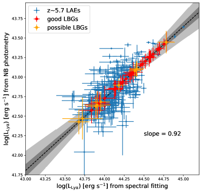
We measure the Lyline flux of each LBG by integrating the best-fit Lymodel profile and applying a correction. Line flux directly calculated from an observed line in faint targets (like our LBGs) can be significantly underestimated due to several reasons, such as fiber loss, alignment problems, skyline contamination, etc. For narrowband-selected LAEs, their Lyline flux can be well determined using the combination of spectroscopic redshifts, narrowband photometry, and broadband photometry. This has been applied to the LAEs in our fields (Ning et al., 2020, 2022). For 260 LAEs at in our fields, we compare their Lyflux derived from the photometric data and from the best-fit Lyline profiles, and the result is shown in Figure 4. We use a hierarchical Bayesian method to do a linear regression on the Lyluminosities calculated by these two methods, considering the errors on both axes. The best-fit function is depicted by the black dashed line in Figure 4, and the and confidence intervals are shown in the shaded regions. Given that these LAEs and the LBGs in this work are in the same fields and were observed at the same time, the LBGs in our sample should follow the same relation. We apply this relation to measure the line flux of our LBGs, and the measured Lyluminosities L(Ly) are listed in Column 8 of Table 2. The IGM absorption blueward of Lyis not considered.
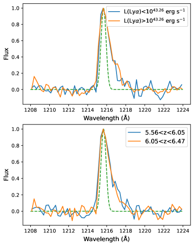
We use LBGs in the ‘good’ sample to study the dependence of the Lyline width (full width at half maximum, or FWHM) on redshift and Lyluminosity. We exclude three galaxies whose Lylines are likely largely affected by strong residuals of the sky subtraction. We then divide the remaining galaxies into two Lyluminosity bins, and produce a stacked spectrum for each bin. We adjust the number of spectra in each bin so that the two stacked spectra have similar S/N . The result is shown in the upper panel of Figure 5. We also produce two stacked spectra for two redshift bins using the same method, and the result is shown in the lower panel of Figure 5. The figure does not show apparent dependence of the line FWHM on redshift or luminosity. Using a large sample of LAEs at and 6.6, Ning et al. (2020, 2022) found that more luminous galaxies tend to have higher LyFWHMs, because more massive host halos possess higher HI column densities and higher gas velocities. We do not see this trend in our LBG sample, likely because the line shape has been severely affected by OH skylines. Unlike LAEs at and 6.6, the Lylines of the LBGs in our sample are often contaminated by skylines.
4 Properties of the LBGs
4.1 UV slopes and LyEWs
In this section, we collect multi-wavelength observations to study the physical properties and stellar populations of the LBGs in our sample. We make use of the following data, including the Hyper Suprime-Cam Subaru Strategic Program (HSC-SSP, Aihara et al. 2022), the UKIRT Infrared Deep Sky Survey (UKIDSS, Lawrence et al. 2007), the Great Observatories Origins Deep Survey (GOODS, Giavalisco et al. 2004), the VISTA Deep Extragalactic Observations Survey (VIDEO, Jarvis et al. 2013), the Cosmic Assembly Near-IR Deep Extragalactic Legacy Survey (CANDELS, Grogin et al. 2011; Koekemoer et al. 2011), and the Cosmic Dawn Survey by Spitzer Space Telescope (only the 3.6, 4.5 data are used, Euclid Collaboration et al. 2022). The No. 13 LBG is covered by the JWST Cycle-1 program (GO 1837), Public Release IMaging for Extragalactic Research (PRIMER, Dunlop et al. 2021), and has NIRCam imaging in eight bands (F090W, F115W, F150W, F200W, F277W, F356W, F410M, and F444W). Ning et al. (2022) carried out a pilot study of seven spectroscopically confirmed LBGs, including No. 13 LBG, using the JWST NIRCam imaging data. The No. 7 LBG is covered by another JWST Cycle-1 program COSMOS-Web (GO 1727, Casey et al. 2022), and has NIRCam imaging in four bands (F115W, F150W, F277W, and F444W).
Most LBGs in our sample except those in the A370a field have multi-wavelength data that can be used to determine UV continuum slope and other physical properties via SED modeling. The IRAC images of many LBGs are blended with nearby sources. In this case, GALFIT (Peng et al., 2002, 2010) is used to model and subtract contaminant sources. Photometry of the target is then done after the de-blending.
We then measure and the absolute UV magnitude (at rest-frame 1500 Å) for the LBGs using the near-IR data mentioned above. The median value is , which is consistent with the median for LBGs within the absolute magnitude bin mag from Bouwens et al. (2014). We also measure the UV slopes of bright LAEs at in Ning et al. (2020) and find a median value of , which is consistent with the value for the LBGs in this sample. For the LBGs in A370a that do not have near-IR data, we use the band photometry to estimate the UV continuum flux. Since we are not able to determine , we adopt the median from the other fields. For simplicity, we assume that the flux blueward of Lyis completely absorbed. If a Lyline is in the band, its flux is subtracted from the -band photometry. The calculated and Lyrest-frame EW values are listed in Columns 9 and 10 of Table 2.
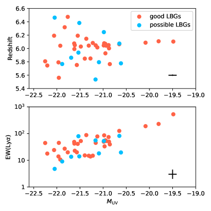
Figure 6 shows the distribution of the LBG redshifts and LyEWs with respect to in our sample. These LBGs span a UV magnitude range of to mag, corresponding to times the characteristic luminosity of galaxies at (Bouwens et al., 2021), and a Lyluminosity range of erg s-1. They represent the most luminous galaxies at in terms of both UV continuum luminosity and Lyluminosity.
4.2 Stellar populations
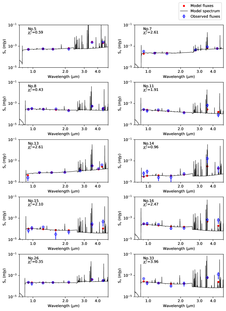
Ten LBGs in the ‘good’ sample have sufficient multi-wavelength imaging data (especially IRAC and photometry) that allow us to perform SED modeling. We model their SEDs and derive their stellar populations using the Code Investigating GALaxy Emission (CIGALE; Noll et al. 2009). Our spectroscopic redshifts remove one critical free parameter in the fitting process. We use the stellar population synthesis models of Bruzual & Charlot (2003) and adopt the Salpeter initial mass function. Given the limited number of available photometric data points, we use as few free parameters as possible. We use constant SFRs and fix metallicity to be 0.2 . A nebular emission template based on Inoue (2011) is included, with ionization parameter , metallicity, and line width fixed. We do not include AGN components during the model fitting because these LBGs do not show any AGN features in the observed bands. Furthermore, Lyemission and radiative transfer in galaxies are very complex (e.g., Charlot & Fall 1993). Our LBGs are among galaxies with the strongest Lyemission, and the nebular emission model built in CIGALE can not reproduce the Lyemission in the SEDs of many LBGs unless we assume an extremely young stellar population (see Section 5.2). Therefore, we mask out the Lyline in the nebular template of CIGALE when fitting and subtracting the Lycontribution from the broadband photometry.
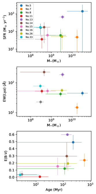
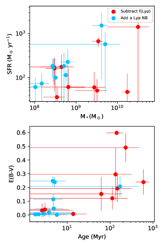
We mainly constrain stellar mass , age, star formation rate (SFR), and dust reddening . We use the dust extinction law of Calzetti et al. (2000) with in a range of . We allow age to vary between 1 and 800 Myr (the age of the Universe at is 914 Myr). The distributions of the derived properties are shown in Figure 7 and the SED modeling results are shown in Figure 8. As seen from the figures, the derived values of the properties all span wide ranges, indicating that these LBGs have a variety of stellar populations. The LBGs are strongly star-forming galaxies with SFRs roughly between 30 and 1000 yr-1. While most of them have SFRs around 100 yr-1, two LBGs, (No. 5 and No. 13) have SFRs close to 1000 yr-1. This is not surprising, because No. 5 is very luminous with mag and No. 13 is also luminous ( mag) with a very high LyEW ( Å). The two galaxies also have high stellar masses, relatively large ages, and relatively high dust extinction. No. 13 has been observed by JWST NIR-Cam and will be further discussed later.
Observational studies of stellar populations in Lygalaxies have suggested that young and low-mass galaxies tend to hold Lylines with large EWs (e.g., Ono et al., 2010; Hayes et al., 2023; Roy et al., 2023). This can be explained by increasing gas and dust content in more massive galaxies and thus lower Lyescape fractions, or intrinsically low Lyproduction by more evolved populations. The middle panel of Figure 8 shows that our galaxies generally follow this trend that less massive galaxies having higher LyEWs
4.3 Galaxy Morphology
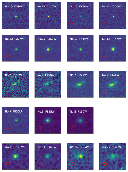
Two LBGs in our sample (No. 7 and No. 13) have high-resolution JWST NIRCam images, and three LBGs (No. 5, No. 11, and No. 26) have HST WFC3 near-IR images. The JWST images are retrieved from the Mikulski Archive for Space Telescopes (MAST) and then reduced by the JWST Calibration Pipeline (version 1.11.4). We basically follow the procedure of the CEERS team for the image reduction (Finkelstein et al., 2023). The final resampled and combined images have a pixel scale of for the short wavelengths (SW; F090W, F115W, F150W, and F200W) and for the long wavelengths (LW; F277W, F356W, F410M, and F444W). The HST data of the three LBGs are from the CANDELS survey and the images are downloaded from the website111https://archive.stsci.edu/hlsp/candels. The cutout images of the five LBGs are shown in Figure 9.
We measure morphological parameters for the five LBGs using GALFIT. For either of the two LBGs with NIRCam images, we stack its SW images and its LW images to produce two combined images. This is to increase S/N, assuming that the object morphology and image quality are similar in individual input bands. Likewise, we stack the F125W and F160W images for each of the three LBGs with HST data. A PSF is obtained for each combined image by stacking several unsaturated stars in the same image, and the resultant FWHM of PSFs are shown as the red circles in Figure 9. The FWHM values of the PSFs in the NIRCam SW and LW bands are about and ( and 0.84 kpc at ) , respectively. The PSF FWHM of the HST images is about ( kpc at ).
We then use GALFIT to model the galaxies on the stacked images, and constrain a few basic parameters, including the effective radius along the major axis, index (allowed to vary between 0.3 and 4), and projected minor-to-major axis ratio (). We find that all galaxies except No. 7 can be well fitted by one profile. No. 7 LBG seems to have two separate components and will be further discussed later. The fitting results of the profiles are reported in Table 3.
| No. | bands | (kpc) | ||
|---|---|---|---|---|
| 13 | F090W, F115W, F150W, F200W | |||
| F277W, F356W, F410M, F444W | ||||
| F115W, F150W | ||||
| F277W, F444W | ||||
| 5 | F125W, F160W | |||
| 11 | F125W, F160W | |||
| 26 | F125W, F160W |
Note. — a. The parameters of profile of the main component is reported.
Figure 9 and Table 3 show that most galaxies in our sample are compact. For example, No. 13 is barely resolved. Its effective radius is kpc in the SW bands and kpc in the LW bands, making it one of the most compact galaxies in this redshift and luminosity range (see, e.g., Sun et al. 2023). Its large LyEW, high SFR, and compact size is consistent with Green Pea (GP) galaxies found at low redshift (Cardamone et al., 2009) that likely have compact star-forming regions embedded in diffuse, older stellar components (Amorín et al., 2012; Clarke et al., 2021). The GP galaxies are thought to have numerous counterparts at the reionization epoch and some of them may have been discovered recently by JWST (Hall, 2023; Rhoads et al., 2023). Studies of local GP galaxies have provided valuable information on how Lyphotons escape from ISM and CGM, which help us better understand their high-redshift counterparts (e.g., Henry et al., 2015; Yang et al., 2017). Another possible explanation for the compactness of the No. 13 galaxy is that this galaxy holds an AGN that partly powers its strong Lyemission.
No. 7 LBG has a quite extended structure and appears to show two components, including a major component and a much weaker component to the north-west of the major one. The major component is more than five times brighter than the minor component in all four bands, so the major component dominates the radiation in these bands. It is unclear whether the weak component is part of the galaxy or a foreground object. In addition, mergers and interacting systems occur more frequently at high redshift (Rodriguez-Gomez et al., 2015), so it is possible that No. 7 LBG is a merger. To verify that the two components belong to the same source, we estimate the probability that the distance between any two random sources is less than the distance between the two components of No. 7 LBG (). Based on the NIRCam images used above, we find that the probability is only 0.02, suggesting that the minor component is unlikely a foreground object. Therefore, we use an additional single profile to model the minor component of No. 7, and we obtain a much better fitting result. Table 3 shows the result for the major component.
5 Discussion
5.1 Fraction of Lyemitters in LBGs
The fraction of LAEs among LBGs is an important tracer of the IGM state during the epoch of reionization, and many works have been done to constrain the fraction of the neutral hydrogen and its redshift evolution. This method is also called the Lyvisibility test. Previous studies have shown that the fraction of LAEs in LBG samples increases steadily from low redshift to , and drops dramatically towards higher redshift (e.g., Stark et al., 2010, 2011; Ono et al., 2012; Bian et al., 2015). It is difficult to explain this using a sudden change in the physical properties of galaxies, but it can be easily explained by the increase of the fraction of the neutral hydrogen in the IGM that attenuates Lyemission. Before we calculate the LAE fraction in our LBG sample, we would like to clarify the definitions of LAEs and LBGs since the definitions are slightly different in the literature. LBGs mean galaxies selected by the Lyman-break technique, regardless of the existence of Lyemission. For LBGs at , they are usually very faint, and spectroscopic identifications primarily rely on their Lyemission. This means that spectroscopically confirmed LBGs typically have strong Lyemission, and also means that the vast majority of the known LBGs at are not spectroscopically confirmed (or just candidates). LAEs are galaxies with strong Lyemission (typically EW or 50 Å). Narrowband-selected galaxies are mostly LAEs by definition. If an LBG has strong Lyemission, it is also an LAE, meaning that most spectroscopically confirmed LBGs to date are also LAEs. In the following analyses, we use EW Å to define LAEs.
We measure the LAE fraction among LBGs at using our spectroscopically confirmed LBG sample. As mentioned earlier, our LBG selection criteria are slightly looser than those used in previous studies, which may result in a slightly higher contamination rate. Therefore, our result can be regarded as a lower limit. Because of the presence of strong OH skylines in the wavelength range that we probe, the identification of the Lyline is incomplete. We run simulations to estimate the completeness for the Lyline identification in the spectra. We generate a grid of model Lylines with a range of redshifts – and line strengths – using the Lytemplate from Ning et al. (2020). For each spectrum without a Lydetection, we insert an artificial Lyline. We then search for these lines using the same method that was used for real spectra in Section 3.1. The derived completeness function is the recovery rate of the lines in each redshift and Lyluminosity bin.
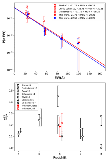
We then apply the completeness correction to the LAE fraction and the result is shown in Figure 10. The upper panel of the figure shows the cumulative distribution of the Lyrest-frame EWs in the ‘good’ LBG sample. The fraction in a fainter subsample ( mag) is marginally higher than that in the whole LBG sample ( mag). The results are generally consistent with previous studies (Pentericci et al., 2011; Stark et al., 2011; Curtis-Lake et al., 2012; De Barros et al., 2017).
In the lower panel of Figure 10, we show the LAE fractions in both ‘good’ and the whole samples, and compare them with previous studies (Stark et al., 2011; Curtis-Lake et al., 2012; Ono et al., 2012; Schenker et al., 2014; Tilvi et al., 2014; Cassata et al., 2015; De Barros et al., 2017) in a redshift range of . The UV magnitude range of the LBGs is mag, which corresponds to the fainter part of our sample and the brighter part of the previous samples. As seen from the figure, our result is broadly consistent with previous results, albeit with a large scatter. The large scatter and error bars reflect complex sample bias and incompleteness. The figure also shows that increases from lower redshifts to and then decreases towards higher redshifts, consistent with the previous claim. The mild decline of may suggest that the evolution of the IGM opacity from to is not very dramatic, if the Lyvisibility mostly depends on the IGM state. Nevertheless, larger and more complete samples are needed.
5.2 SED modeling with strong Lyemission
In Section 4.2 when we modeled the SEDs of the LBGs, we did not consider the Lyemission due to its complexity. Here we discuss how the results change if we consider the Lyemission in our SED modeling. As has been pointed out, the SED modeling for galaxies has a strong degeneracy between young galaxies with prominent nebular emission and old galaxies with strong Balmer breaks (e.g., Jiang et al., 2015). To include the Lyemission, we make a pseudo narrowband filter with a spectral resolving power of at the wavelength of Lyfor each LBG. The narrowband photometry is then calculated from the Lyflux and implemented for SED modeling. In the modeling procedure, the ionization parameter , gas metallicity in the nebular emission model, and the ratio of continuum to line reddening are considered as free parameters.
The derived properties of the stellar populations and the comparison with the previous results from Section 4.2 are shown in Figure 11. The best-fit values of the two methods are about the same. Figure 11 clearly shows that when the Lyemission is considered in the SED modeling procedure, these galaxies are much younger with significantly lower stellar masses. The reason is straightforward. In order to produce strong Lyemission seen in the galaxies, the stellar populations must be very young with high SFRs, which further results in lower stellar masses. It should be noted, however, that it is difficult to decide how to include the Lyemission for SED modeling due to the complexity of the Lyemission. For example, the measurement of the Lyflux is almost always a lower limit, this is mainly because the resonant scattering of the Lyphotons often forms a large diffuse halo, but the actual measurement is usually done on the central part. It is also because the Lyescape fraction varies a lot among galaxies. In addition, there are other sources of uncertainties that are particularly important for galaxies, including the variation of the IGM absorption along the line-of-sights.
5.3 Search for AGN activity
The LBGs in our sample have strong Lyand UV continuum emission. In addition, some of them are morphologically very compact. It is possible that they harbor a central AGN that partly contributes to the total emission. We search for possible evidence of AGN activity in these galaxies. First of all, they do not have typical Type I AGN components, as seen from their narrow Lyemission lines. Figure 5 shows that the stacked Lyline displays a narrow profile with a velocity dispersion of km/s (IGM absorption is neglected here), which is much smaller than those in typical broad-line AGN ( km/s).
The wavelength coverage of our spectra is from 7600 Å to 9600 Å, corresponding to a rest-frame range of 1090-1370 Å for objects. This range covers the N V 1240 Å emission line that is often regarded as evidence of the presence of AGN. We do not detect any N V emission in the combined spectrum of the LBGs. For a typical AGN, however, the N V flux is only a few percent of the Lyflux (e.g., Vanden Berk et al., 2001), so even if any of our LBGs contain an AGN component, its N V flux is below our detection limit.
We also check these galaxies in deep Chandra X-ray images, including the Chandra Deep Field-South field (CDF-S) (Luo et al., 2017), the UKIDSS Ultra Deep Survey Field (Kocevski et al., 2018), and the Chandra Cosmos Legacy Survey field (Civano et al., 2016). None of them is individually detected. X-ray detections were actually excluded in the first steps of the target selection. The No.5 and No.6 LBGs are in the 7 Ms CDF-S field, and their stacked image have an effective exposure time of over 12 Ms. For the stacked 0.5–7 keV image, we measure the X-ray photon counts in a radius aperture, which encloses of the total energy at 6.4 keV. The background counts are computed in an annular region with the inner and outer radii of and . The error of the net counts is calculated based on the Poisson errors on the extracted source and background counts. The calculated upper limit is 6.3 counts. To estimate the upper limit of a possible X-ray detection, we assume a typical type 1 quasar with a similar UV magnitude at the same redshift as the No.5 and No.6 LBGs (, mag). We also assume the Shen et al. (2020) SED template for the quasar. We adopt the Galactic neutral hydrogen column density along the line-of-sight to the CDF-S (Stark et al., 1992). No other absorption is applied. In this case, the 12 Ms exposure would yield a detection (19.2 counts in 0.5–7 keV band) for this quasar. This simple calculation means that AGN contributes less than one-third ( upper limit) of the total luminosity in the two LBGs. Therefore, we are not able to rule out the possibility of weaker AGN activities in these galaxies. The stacked images in another two fields are much shallower and thus cannot provide useful constraints.
6 Summary
We have presented a sample of 45 spectroscopically confirmed LBGs at in four well-studied fields, including SXDS, A370, ECDFS, and COSMOS. This sample is one of the largest samples of spectroscopically confirmed LBGs at this redshift. The LBG candidates were selected as -band dropout objects from deep broadband images. The spectroscopic observations were carried out using M2FS on the Magellan Clay telescope. We identified the Lylines of the galaxies based on their 1D and 2D M2FS spectra. Their redshifts and Lyluminosities were measured by fitting a composite Lyline template to the individual 1D spectra. The absolute UV magnitude and UV slope were calculated by fitting a power-law to the available multi-wavelength photometric data. The UV absolute magnitudes of these LBGs are between –22.5 and –19.0 mag, corresponding to times the characteristic luminosity of galaxies at , with a LyEW range from 10 Å to 400 Å. They represent the most UV luminous galaxies known at .
The SED modeling of ten LBGs in the sample reveals that they have a wide range of stellar masses and ages with high SFRs. We note that whether to consider the Lyemission in the SED modeling procedure has a significant impact on the measurement of the stellar populations in these galaxies, indicating the complexity of the Lyemission. Five LBGs have high-resolution JWST NIRCam images or HST WFC3 near-IR images. Four of them show compact morphology, and one appears to have two components that might be a merger. We calculated the LAE fraction among the photometrically selected LBGs after correcting for the Ly-identification completeness. The fraction of is consistent with previous works, and it supports a moderate evolution of the IGM opacity at the end of cosmic reionization when previous results at lower and higher redshifts were combined. Finally, we did not find evidence of strong AGN activities in these galaxies.
References
- Aihara et al. (2022) Aihara, H., AlSayyad, Y., Ando, M., et al. 2022, Publications of the Astronomical Society of Japan, 74, 247, doi: 10.1093/pasj/psab122
- Amorín et al. (2012) Amorín, R., Pérez-Montero, E., Vílchez, J. M., & Papaderos, P. 2012, ApJ, 749, 185, doi: 10.1088/0004-637X/749/2/185
- Arrabal Haro et al. (2023) Arrabal Haro, P., Dickinson, M., Finkelstein, S. L., et al. 2023, arXiv e-prints, arXiv:2303.15431, doi: 10.48550/arXiv.2303.15431
- Astropy Collaboration et al. (2013) Astropy Collaboration, Robitaille, T. P., Tollerud, E. J., et al. 2013, A&A, 558, A33, doi: 10.1051/0004-6361/201322068
- Astropy Collaboration et al. (2018) Astropy Collaboration, Price-Whelan, A. M., Sipőcz, B. M., et al. 2018, AJ, 156, 123, doi: 10.3847/1538-3881/aabc4f
- Astropy Collaboration et al. (2022) Astropy Collaboration, Price-Whelan, A. M., Lim, P. L., et al. 2022, apj, 935, 167, doi: 10.3847/1538-4357/ac7c74
- Atek et al. (2023) Atek, H., Chemerynska, I., Wang, B., et al. 2023, MNRAS, 524, 5486, doi: 10.1093/mnras/stad1998
- Bian et al. (2015) Bian, F., Stark, D. P., Fan, X., et al. 2015, ApJ, 806, 108, doi: 10.1088/0004-637X/806/1/108
- Bouwens et al. (2014) Bouwens, R. J., Illingworth, G. D., Oesch, P. A., et al. 2014, The Astrophysical Journal, 793, 115, doi: 10.1088/0004-637X/793/2/115
- Bouwens et al. (2021) Bouwens, R. J., Oesch, P. A., Stefanon, M., et al. 2021, The Astronomical Journal, 162, 47, doi: 10.3847/1538-3881/abf83e
- Bruzual & Charlot (2003) Bruzual, G., & Charlot, S. 2003, MNRAS, 344, 1000, doi: 10.1046/j.1365-8711.2003.06897.x
- Bunker et al. (2023) Bunker, A. J., Cameron, A. J., Curtis-Lake, E., et al. 2023, arXiv e-prints, arXiv:2306.02467, doi: 10.48550/arXiv.2306.02467
- Calzetti et al. (2000) Calzetti, D., Armus, L., Bohlin, R. C., et al. 2000, ApJ, 533, 682, doi: 10.1086/308692
- Cardamone et al. (2009) Cardamone, C., Schawinski, K., Sarzi, M., et al. 2009, MNRAS, 399, 1191, doi: 10.1111/j.1365-2966.2009.15383.x
- Casey et al. (2022) Casey, C. M., Kartaltepe, J. S., Drakos, N. E., et al. 2022, arXiv e-prints, arXiv:2211.07865, doi: 10.48550/arXiv.2211.07865
- Cassata et al. (2015) Cassata, P., Tasca, L. A. M., Le Fèvre, O., et al. 2015, Astronomy & Astrophysics, 573, A24, doi: 10.1051/0004-6361/201423824
- Castellano et al. (2017) Castellano, M., Pentericci, L., Fontana, A., et al. 2017, The Astrophysical Journal, 839, 73, doi: 10.3847/1538-4357/aa696e
- Champagne et al. (2023) Champagne, J. B., Casey, C. M., Finkelstein, S. L., et al. 2023, ApJ, 952, 99, doi: 10.3847/1538-4357/acda8d
- Charlot & Fall (1993) Charlot, S., & Fall, S. M. 1993, ApJ, 415, 580, doi: 10.1086/173187
- Civano et al. (2016) Civano, F., Marchesi, S., Comastri, A., et al. 2016, ApJ, 819, 62, doi: 10.3847/0004-637X/819/1/62
- Clarke et al. (2021) Clarke, L., Scarlata, C., Mehta, V., et al. 2021, ApJ, 912, L22, doi: 10.3847/2041-8213/abf7cc
- Curtis-Lake et al. (2012) Curtis-Lake, E., McLure, R. J., Pearce, H. J., et al. 2012, Monthly Notices of the Royal Astronomical Society, 422, 1425, doi: 10.1111/j.1365-2966.2012.20720.x
- Curtis-Lake et al. (2016) Curtis-Lake, E., McLure, R. J., Dunlop, J. S., et al. 2016, Monthly Notices of the Royal Astronomical Society, 457, 440, doi: 10.1093/mnras/stv3017
- Curtis-Lake et al. (2023) Curtis-Lake, E., Carniani, S., Cameron, A., et al. 2023, Nature Astronomy, 7, 622, doi: 10.1038/s41550-023-01918-w
- De Barros et al. (2017) De Barros, S., Pentericci, L., Vanzella, E., et al. 2017, A&A, 608, A123, doi: 10.1051/0004-6361/201731476
- Dunlop et al. (2012) Dunlop, J. S., McLure, R. J., Robertson, B. E., et al. 2012, Monthly Notices of the Royal Astronomical Society, 420, 901, doi: 10.1111/j.1365-2966.2011.20102.x
- Dunlop et al. (2021) Dunlop, J. S., Abraham, R. G., Ashby, M. L. N., et al. 2021, 1837
- Egami et al. (2005) Egami, E., Kneib, J.-P., Rieke, G. H., et al. 2005, The Astrophysical Journal, 618, L5, doi: 10.1086/427550
- Euclid Collaboration et al. (2022) Euclid Collaboration, Moneti, A., McCracken, H. J., et al. 2022, A&A, 658, A126, doi: 10.1051/0004-6361/202142361
- Faisst et al. (2016) Faisst, A. L., Capak, P., Hsieh, B. C., et al. 2016, The Astrophysical Journal, 821, 122, doi: 10.3847/0004-637X/821/2/122
- Finkelstein et al. (2012a) Finkelstein, S. L., Papovich, C., Salmon, B., et al. 2012a, The Astrophysical Journal, 756, 164, doi: 10.1088/0004-637X/756/2/164
- Finkelstein et al. (2012b) Finkelstein, S. L., Papovich, C., Ryan, R. E., et al. 2012b, The Astrophysical Journal, 758, 93, doi: 10.1088/0004-637X/758/2/93
- Finkelstein et al. (2013) Finkelstein, S. L., Papovich, C., Dickinson, M., et al. 2013, Nature, 502, 524, doi: 10.1038/nature12657
- Finkelstein et al. (2023) Finkelstein, S. L., Bagley, M. B., Ferguson, H. C., et al. 2023, ApJ, 946, L13, doi: 10.3847/2041-8213/acade4
- Fujimoto et al. (2023) Fujimoto, S., Arrabal Haro, P., Dickinson, M., et al. 2023, ApJ, 949, L25, doi: 10.3847/2041-8213/acd2d9
- Giavalisco et al. (2004) Giavalisco, M., Ferguson, H. C., Koekemoer, A. M., et al. 2004, ApJ, 600, L93, doi: 10.1086/379232
- González et al. (2014) González, V., Bouwens, R., Illingworth, G., et al. 2014, The Astrophysical Journal, 781, 34, doi: 10.1088/0004-637X/781/1/34
- Grogin et al. (2011) Grogin, N. A., Kocevski, D. D., Faber, S. M., et al. 2011, ApJS, 197, 35, doi: 10.1088/0067-0049/197/2/35
- Guaita et al. (2015) Guaita, L., Melinder, J., Hayes, M., et al. 2015, Astronomy and Astrophysics, 576, A51, doi: 10.1051/0004-6361/201425053
- Hall (2023) Hall, S. 2023, Nature, 613, 425, doi: 10.1038/d41586-023-00064-7
- Hayes et al. (2023) Hayes, M. J., Runnholm, A., Scarlata, C., Gronke, M., & Rivera-Thorsen, T. E. 2023, MNRAS, 520, 5903, doi: 10.1093/mnras/stad477
- Henry et al. (2015) Henry, A., Scarlata, C., Martin, C. L., & Erb, D. 2015, ApJ, 809, 19, doi: 10.1088/0004-637X/809/1/19
- Hsiao et al. (2023) Hsiao, T. Y.-Y., Coe, D., Abdurro’uf, et al. 2023, ApJ, 949, L34, doi: 10.3847/2041-8213/acc94b
- Hu et al. (2010) Hu, E. M., Cowie, L. L., Barger, A. J., et al. 2010, The Astrophysical Journal, 725, 394, doi: 10.1088/0004-637X/725/1/394
- Inoue (2011) Inoue, A. K. 2011, MNRAS, 415, 2920, doi: 10.1111/j.1365-2966.2011.18906.x
- Inoue et al. (2014) Inoue, A. K., Shimizu, I., Iwata, I., & Tanaka, M. 2014, MNRAS, 442, 1805, doi: 10.1093/mnras/stu936
- Jarvis et al. (2013) Jarvis, M. J., Bonfield, D. G., Bruce, V. A., et al. 2013, MNRAS, 428, 1281, doi: 10.1093/mnras/sts118
- Jiang et al. (2015) Jiang, L., Finlator, K., Cohen, S. H., et al. 2015, The Astrophysical Journal, 816, 16, doi: 10.3847/0004-637X/816/1/16
- Jiang et al. (2017) Jiang, L., Shen, Y., Bian, F., et al. 2017, The Astrophysical Journal, 846, 134, doi: 10.3847/1538-4357/aa8561
- Jiang et al. (2018) Jiang, L., Wu, J., Bian, F., et al. 2018, Nature Astronomy, 2, 962, doi: 10.1038/s41550-018-0587-9
- Jiang et al. (2022) Jiang, L., Ning, Y., Fan, X., et al. 2022, Nature Astronomy, 6, 850, doi: 10.1038/s41550-022-01708-w
- Jung et al. (2018) Jung, I., Finkelstein, S. L., Livermore, R. C., et al. 2018, The Astrophysical Journal, 864, 103, doi: 10.3847/1538-4357/aad686
- Jung et al. (2022) Jung, I., Papovich, C., Finkelstein, S. L., et al. 2022, The Astrophysical Journal, 933, 87, doi: 10.3847/1538-4357/ac6fe7
- Karman et al. (2017) Karman, W., Caputi, K. I., Caminha, G. B., et al. 2017, Astronomy & Astrophysics, 599, A28, doi: 10.1051/0004-6361/201629055
- Kashikawa et al. (2006) Kashikawa, N., Shimasaku, K., Malkan, M. A., et al. 2006, The Astrophysical Journal, 648, 7, doi: 10.1086/504966
- Kawamata et al. (2015) Kawamata, R., Ishigaki, M., Shimasaku, K., Oguri, M., & Ouchi, M. 2015, The Astrophysical Journal, 804, 103, doi: 10.1088/0004-637X/804/2/103
- Kobayashi et al. (2016) Kobayashi, M. A. R., Murata, K. L., Koekemoer, A. M., et al. 2016, The Astrophysical Journal, 819, 25, doi: 10.3847/0004-637X/819/1/25
- Kocevski et al. (2018) Kocevski, D. D., Hasinger, G., Brightman, M., et al. 2018, ApJS, 236, 48, doi: 10.3847/1538-4365/aab9b4
- Koekemoer et al. (2011) Koekemoer, A. M., Faber, S. M., Ferguson, H. C., et al. 2011, ApJS, 197, 36, doi: 10.1088/0067-0049/197/2/36
- Larson et al. (2022) Larson, R. L., Finkelstein, S. L., Hutchison, T. A., et al. 2022, The Astrophysical Journal, 930, 104, doi: 10.3847/1538-4357/ac5dbd
- Lawrence et al. (2007) Lawrence, A., Warren, S. J., Almaini, O., et al. 2007, MNRAS, 379, 1599, doi: 10.1111/j.1365-2966.2007.12040.x
- Leethochawalit et al. (2023) Leethochawalit, N., Trenti, M., Santini, P., et al. 2023, ApJ, 942, L26, doi: 10.3847/2041-8213/ac959b
- Liu et al. (2017) Liu, C., Mutch, S. J., Poole, G. B., et al. 2017, Monthly Notices of the Royal Astronomical Society, 465, 3134, doi: 10.1093/mnras/stw2912
- Luo et al. (2017) Luo, B., Brandt, W. N., Xue, Y. Q., et al. 2017, ApJS, 228, 2, doi: 10.3847/1538-4365/228/1/2
- Mascia et al. (2023) Mascia, S., Pentericci, L., Calabrò, A., et al. 2023, A&A, 672, A155, doi: 10.1051/0004-6361/202345866
- Mateo et al. (2012) Mateo, M., Bailey, J. I., Crane, J., et al. 2012, 84464Y, doi: 10.1117/12.926448
- Matthee et al. (2023) Matthee, J., Mackenzie, R., Simcoe, R. A., et al. 2023, ApJ, 950, 67, doi: 10.3847/1538-4357/acc846
- McLeod et al. (2016) McLeod, D. J., McLure, R. J., & Dunlop, J. S. 2016, Monthly Notices of the Royal Astronomical Society, 459, 3812, doi: 10.1093/mnras/stw904
- Naidu et al. (2022) Naidu, R. P., Oesch, P. A., van Dokkum, P., et al. 2022, ApJ, 940, L14, doi: 10.3847/2041-8213/ac9b22
- Ning et al. (2022) Ning, Y., Cai, Z., Jiang, L., et al. 2022, arXiv e-prints, arXiv:2211.13620. https://arxiv.org/abs/2211.13620
- Ning et al. (2022) Ning, Y., Jiang, L., Zheng, Z.-Y., & Wu, J. 2022, The Astrophysical Journal, 926, 230, doi: 10.3847/1538-4357/ac4268
- Ning et al. (2020) Ning, Y., Jiang, L., Zheng, Z.-Y., et al. 2020, The Astrophysical Journal, 903, 4, doi: 10.3847/1538-4357/abb705
- Noll et al. (2009) Noll, S., Burgarella, D., Giovannoli, E., et al. 2009, A&A, 507, 1793, doi: 10.1051/0004-6361/200912497
- Oesch et al. (2023) Oesch, P. A., Brammer, G., Naidu, R. P., et al. 2023, MNRAS, 525, 2864, doi: 10.1093/mnras/stad2411
- Ono et al. (2010) Ono, Y., Ouchi, M., Shimasaku, K., et al. 2010, MNRAS, 402, 1580, doi: 10.1111/j.1365-2966.2009.16034.x
- Ono et al. (2012) Ono, Y., Ouchi, M., Mobasher, B., et al. 2012, The Astrophysical Journal, 744, 83, doi: 10.1088/0004-637X/744/2/83
- Ono et al. (2018) Ono, Y., Ouchi, M., Harikane, Y., et al. 2018, Publications of the Astronomical Society of Japan, 70, doi: 10.1093/pasj/psx103
- Onoue et al. (2017) Onoue, M., Kashikawa, N., Willott, C. J., et al. 2017, The Astrophysical Journal, 847, L15, doi: 10.3847/2041-8213/aa8cc6
- Oyarzún et al. (2017) Oyarzún, G. A., Blanc, G. A., González, V., Mateo, M., & Bailey, J. I. 2017, The Astrophysical Journal, 843, 133, doi: 10.3847/1538-4357/aa7552
- Oyarzún et al. (2016) Oyarzún, G. A., Blanc, G. A., González, V., et al. 2016, The Astrophysical Journal, 821, L14, doi: 10.3847/2041-8205/821/1/L14
- Peng et al. (2002) Peng, C. Y., Ho, L. C., Impey, C. D., & Rix, H.-W. 2002, AJ, 124, 266, doi: 10.1086/340952
- Peng et al. (2010) —. 2010, AJ, 139, 2097, doi: 10.1088/0004-6256/139/6/2097
- Pentericci et al. (2011) Pentericci, L., Fontana, A., Vanzella, E., et al. 2011, The Astrophysical Journal, 743, 132, doi: 10.1088/0004-637X/743/2/132
- Prieto-Lyon et al. (2023) Prieto-Lyon, G., Mason, C., Mascia, S., et al. 2023, ApJ, 956, 136, doi: 10.3847/1538-4357/acf715
- Rhoads et al. (2023) Rhoads, J. E., Wold, I. G. B., Harish, S., et al. 2023, ApJ, 942, L14, doi: 10.3847/2041-8213/acaaaf
- Roberts-Borsani et al. (2023) Roberts-Borsani, G., Treu, T., Chen, W., et al. 2023, Nature, 618, 480, doi: 10.1038/s41586-023-05994-w
- Roberts-Borsani et al. (2016) Roberts-Borsani, G. W., Bouwens, R. J., Oesch, P. A., et al. 2016, The Astrophysical Journal, 823, 143, doi: 10.3847/0004-637X/823/2/143
- Robertson et al. (2015) Robertson, B. E., Ellis, R. S., Furlanetto, S. R., & Dunlop, J. S. 2015, The Astrophysical Journal, 802, L19, doi: 10.1088/2041-8205/802/2/L19
- Rodriguez-Gomez et al. (2015) Rodriguez-Gomez, V., Genel, S., Vogelsberger, M., et al. 2015, Monthly Notices of the Royal Astronomical Society, 449, 49, doi: 10.1093/mnras/stv264
- Roy et al. (2023) Roy, N., Henry, A., Treu, T., et al. 2023, ApJ, 952, L14, doi: 10.3847/2041-8213/acdbce
- Schenker et al. (2014) Schenker, M. A., Ellis, R. S., Konidaris, N. P., & Stark, D. P. 2014, ApJ, 795, 20, doi: 10.1088/0004-637X/795/1/20
- Schenker et al. (2012) Schenker, M. A., Stark, D. P., Ellis, R. S., et al. 2012, The Astrophysical Journal, 744, 179, doi: 10.1088/0004-637X/744/2/179
- Schmidt et al. (2016) Schmidt, K. B., Treu, T., Bradač, M., et al. 2016, The Astrophysical Journal, 818, 38, doi: 10.3847/0004-637X/818/1/38
- Shen et al. (2020) Shen, X., Hopkins, P. F., Faucher-Giguère, C.-A., et al. 2020, MNRAS, 495, 3252, doi: 10.1093/mnras/staa1381
- Shibuya et al. (2015) Shibuya, T., Ouchi, M., & Harikane, Y. 2015, The Astrophysical Journal Supplement Series, 219, 15, doi: 10.1088/0067-0049/219/2/15
- Shibuya et al. (2016) Shibuya, T., Ouchi, M., Kubo, M., & Harikane, Y. 2016, The Astrophysical Journal, 821, 72, doi: 10.3847/0004-637X/821/2/72
- Shimasaku et al. (2006) Shimasaku, K., Kashikawa, N., Doi, M., et al. 2006, PASJ, 58, 313, doi: 10.1093/pasj/58.2.313
- Song et al. (2016) Song, M., Finkelstein, S. L., Livermore, R. C., et al. 2016, The Astrophysical Journal, 826, 113, doi: 10.3847/0004-637X/826/2/113
- Stark et al. (1992) Stark, A. A., Gammie, C. F., Wilson, R. W., et al. 1992, ApJS, 79, 77, doi: 10.1086/191645
- Stark et al. (2010) Stark, D. P., Ellis, R. S., Chiu, K., Ouchi, M., & Bunker, A. 2010, Monthly Notices of the Royal Astronomical Society, 408, 1628, doi: 10.1111/j.1365-2966.2010.17227.x
- Stark et al. (2011) Stark, D. P., Ellis, R. S., & Ouchi, M. 2011, ApJ, 728, L2, doi: 10.1088/2041-8205/728/1/L2
- Stark et al. (2011) Stark, D. P., Ellis, R. S., & Ouchi, M. 2011, The Astrophysical Journal, 728, L2, doi: 10.1088/2041-8205/728/1/L2
- Stark et al. (2013) Stark, D. P., Schenker, M. A., Ellis, R., et al. 2013, The Astrophysical Journal, 763, 129, doi: 10.1088/0004-637X/763/2/129
- Sun et al. (2023) Sun, W., Ho, L. C., Zhuang, M.-Y., et al. 2023, The Structure and Morphology of Galaxies during the Epoch of Reionization Revealed by JWST. https://arxiv.org/abs/2308.09076
- Tacchella et al. (2023) Tacchella, S., Johnson, B. D., Robertson, B. E., et al. 2023, MNRAS, 522, 6236, doi: 10.1093/mnras/stad1408
- Tang et al. (2023) Tang, M., Stark, D. P., Chen, Z., et al. 2023, MNRAS, 526, 1657, doi: 10.1093/mnras/stad2763
- Tilvi et al. (2014) Tilvi, V., Papovich, C., Finkelstein, S. L., et al. 2014, The Astrophysical Journal, 794, 5, doi: 10.1088/0004-637X/794/1/5
- Toshikawa et al. (2012) Toshikawa, J., Kashikawa, N., Ota, K., et al. 2012, The Astrophysical Journal, 750, 137, doi: 10.1088/0004-637X/750/2/137
- Vanden Berk et al. (2001) Vanden Berk, D. E., Richards, G. T., Bauer, A., et al. 2001, AJ, 122, 549, doi: 10.1086/321167
- Vanzella et al. (2009) Vanzella, E., Giavalisco, M., Dickinson, M., et al. 2009, ApJ, 695, 1163, doi: 10.1088/0004-637X/695/2/1163
- Vanzella et al. (2014) Vanzella, E., Fontana, A., Pentericci, L., et al. 2014, Astronomy & Astrophysics, 569, A78, doi: 10.1051/0004-6361/201424285
- Wang et al. (2023) Wang, F., Yang, J., Hennawi, J. F., et al. 2023, ApJ, 951, L4, doi: 10.3847/2041-8213/accd6f
- Watson et al. (2015) Watson, D., Christensen, L., Knudsen, K. K., et al. 2015, Nature, 519, 327, doi: 10.1038/nature14164
- Wilkins et al. (2010) Wilkins, S. M., Bunker, A. J., Ellis, R. S., et al. 2010, Monthly Notices of the Royal Astronomical Society, 403, 938, doi: 10.1111/j.1365-2966.2009.16175.x
- Wold et al. (2022) Wold, I. G. B., Malhotra, S., Rhoads, J., et al. 2022, The Astrophysical Journal, 927, 36, doi: 10.3847/1538-4357/ac4997
- Wu et al. (2020) Wu, J., Jiang, L., & Ning, Y. 2020, The Astrophysical Journal, 891, 105, doi: 10.3847/1538-4357/ab7333
- Yan et al. (2023) Yan, H., Sun, B., Ma, Z., & Ling, C. 2023, arXiv e-prints, arXiv:2311.15121, doi: 10.48550/arXiv.2311.15121
- Yang et al. (2017) Yang, H., Malhotra, S., Gronke, M., et al. 2017, ApJ, 844, 171, doi: 10.3847/1538-4357/aa7d4d
- Zheng et al. (2017) Zheng, Z.-Y., Wang, J., Rhoads, J., et al. 2017, The Astrophysical Journal, 842, L22, doi: 10.3847/2041-8213/aa794f