Intermediate-luminosity Type IIP SN 2021gmj: a low-energy explosion with signatures of circumstellar material

Abstract

We present photometric, spectroscopic and polarimetric observations of the intermediate-luminosity Type IIP supernova (SN) 2021gmj from 1 to 386 days after the explosion. The peak absolute $V$-band magnitude of SN 2021gmj is $-15.5$ mag, which is fainter than that of normal Type IIP SNe. The spectral evolution of SN 2021gmj resembles that of other sub-luminous supernovae: the optical spectra show narrow P-Cygni profiles, indicating a low expansion velocity. We estimate the progenitor mass to be about 12 $\rm M_{\odot}$ from the nebular spectrum and the ⁵⁶Ni mass to be about 0.02 $\rm M_{\odot}$ from the bolometric light curve. We also derive the explosion energy to be about 3$\times 10^{50}$ erg by comparing numerical light curve models with the observed light curves. Polarization in the plateau phase is not very large, suggesting nearly spherical outer envelope. The early photometric observations capture the rapid rise of the light curve, which is likely due to the interaction with a circumstellar material (CSM). The broad emission feature formed by highly-ionized lines on top of a blue continuum in the earliest spectrum gives further indication of the CSM at the vicinity of the progenitor. Our work suggests that a relatively low-mass progenitor of an intermediate-luminosity Type IIP SN can also experience an enhanced mass loss just before the explosion, as suggested for normal Type IIP SNe.

1 Introduction

Core-collapse supernovae (CCSNe) are the explosions of massive stars with a zero-age main-sequence (ZAMS) mass of $\gtrsim 8~{}\rm M_{\odot}$ (e.g., Heger et al. 2003). CCSNe with hydrogen lines in their spectra around the maxima of the brightness are classified as Type II SNe (Woosley & Weaver 1986; Filippenko 1997). Among them, SNe that display a plateau feature (Barbon et al. 1979) in their light curves are classified as Type IIP SNe, which are the most common SNe among CCSNe ($\sim 60\%$ of CCSNe; Li et al. 2011).

Many studies have revealed that Type IIP SNe have a wide range of plateau luminosities ($-18\lesssim M_{V\rm,plateau}\lesssim-14~{}\rm mag$, where $M_{V\rm,plateau}$ is the absolute magnitude during the plateau phase in the $V$ band; Anderson et al. 2014; Valenti et al. 2016). The observational diversity of Type IIP SNe has been revealed not only in the luminosity but also in the synthesized ⁵⁶Ni mass ($0.001\lesssim M_{\rm Ni}\lesssim 0.360~{}\rm M_{\odot}$; Müller et al. 2017; Anderson 2019; Rodríguez et al. 2021; Martinez et al. 2022) and the ejecta velocities at 50 days post-explosion ($1,500\lesssim v_{\rm ej}\lesssim 9,600~{}\rm km~{}s^{-1}$; Gutiérrez et al. 2017). In particular, sub-luminous, low-velocity and ⁵⁶Ni-poor Type IIP SNe such as SN 2005cs (Pastorello et al. 2006) have been of interest to understand the variety of the population of Type IIP SNe toward the faintest end. In fact, sub-luminous Type IIP SNe are considered to be lower-energy explosions of lower-mass progenitors as compared to normal Type IIP SNe (Maund et al. 2005; Tsvetkov et al. 2006; Pastorello et al. 2009; Smartt et al. 2009). Moreover, some studies suggest that such sub-luminous SNe can be explained by electron-capture supernovae (Hosseinzadeh et al. 2018; Hiramatsu et al. 2021; Valerin et al. 2022). In addition, Type IIP SNe that have properties lying between those of normal and sub-luminous objects have also been discovered (e.g., SN 2008in, Roy et al. 2011; SN 2009ib, Takáts et al. 2015; SN 2009N, Takáts et al. 2014; SN 2012A, Tomasella et al. 2013).

Recent high-cadence transient surveys enable us to probe the final evolutionary stage of SN progenitors. Rapid photometric observations suggest that a large fraction of massive stars undergo an enhanced mass loss producing extensive circumstellar material (CSM) surrounding these stars in the final years before explosion (e.g., Valenti et al. 2016; Morozova et al. 2017, 2018; Förster et al. 2018). Early spectra observed within a few days after explosion also imply the existence of extensive CSM around the progenitors, showing highly-ionized narrow emission lines produced by photoionization due to the intensive ultraviolet radiation from SNe (Gal-Yam et al. 2014; Smith et al. 2015; Khazov et al. 2016; Yaron et al. 2017). Such early spectra have also been studied for sub-luminous SNe. For instance, Hosseinzadeh et al. (2018) and Nakaoka et al. (2018) reported a feature around 4600 Å in the earliest spectrum of a sub-luminous Type IIP SN 2016bkv, attributing it to He II, C III, and N III originating from CSM. Similarly, the sub-luminous Type IIP SN 2018lab shows such highly-ionized emission lines due to CSM in its early spectra (Pearson et al. 2023). However, the sample of such early observations for intermediate-luminosity or sub-luminous Type IIP SNe are still limited as the observational sample is smaller than normal Type IIP SNe.

The mechanism of the enhanced mass-loss forming such dense CSM has also been under debates. For instance, Yoon & Cantiello (2010) proposed pulsations of red supergiants (RSGs) drive superwinds and result in the enhanced mass loss. Moriya (2014) proposed core neutrino emission shortly before explosion makes luminosity of stars Eddington luminosity, resulting in the enhanced mass loss. Quataert et al. (2016) proposed super-Eddington stellar winds driven by near-surface energy deposition causes the enhanced mass loss. In order to understand the mechanism of the enhanced mass loss, it is important to study the CSM for a variety of supernova progenitors. In fact, some scenarios invoke nuclear flash near the end of stellar evolution, which is expected to be more important for lower-mass progenitors (Woosley & Heger, 2015). Thus, it is of interest to study the CSM around lower-luminosity SNe likely with lower-mass progenitors.

In this paper, we report our photometric, spectroscopic and polarimetric observations for the intermediate-luminosity Type IIP SN 2021gmj from a few days to more than a year after the explosion. In Section 2, we present our observations and data reduction. In Section 3, we show photometric, spectroscopic and polarimetric properties of SN 2021gmj and compare them with those of other Type IIP SNe. In Section 4, we present a detailed analysis with estimates of the ⁵⁶Ni mass, progenitor mass, mass-loss rate, and explosion energy of SN 2021gmj. Finally, we summarize our findings in Section 5.

2 Observation and data reduction

SN 2021gmj was discovered by the Distance Less Than 40 Mpc Survey (DLT40; Tartaglia et al. 2018) at 07:40:48 UTC on 2021-03-20 (59293.32 MJD; Valenti et al. 2021). SN 2021gmj is located at ($\alpha$, $\delta$) = ($10^{\rm h}38^{\rm m}47.345^{\rm s}$, $+53^{\circ}30^{\prime}31.79\arcsec$), with an offset of 19.73$\arcsec$ from the center of its host galaxy, NGC 3310 at a redshift $z=0.003312\pm 0.000009$. The distance to the host galaxy is somewhat uncertain: there are some redshift-independent measurements reported in the NASA/IPAC NED Database, but they are primarily from the Tully-Fisher relation (Bottinelli et al., 1984, 1986). The weighted average distance for these measurements is 19.7 Mpc (distance modulus $\mu=31.47$ mag, Steer 2021), but there is a large dispersion from 17.6 Mpc to 20.2 Mpc. Thus, instead of using these distance estimates, we simply convert the redshift to the luminosity distance of $19.2$ Mpc ($\mu=31.42$ mag), which is obtained in the NED by considering the influence of the Virgo cluster, the Great Attractor (GA), and the Shapley supercluster by assuming $H_{0}$ = 73.0 km $\rm s^{\rm-1}~{}Mpc^{\rm-1}$ (Riess et al. 2022), $\rm\Omega_{m}$ = 0.27 and $\rm\Omega_{\Lambda}$ = 0.73.

Throughout this paper, we show photometry corrected only for the Milky Way extinction ($A_{V}^{\rm MW}$ = 0.0589 mag) assuming $R_{V}$ = 3.1 (Fitzpatrick 1999), based on the Galactic extinction map of Schlafly & Finkbeiner (2011). We do not take the host-galaxy extinction into account as our spectra of SN 2021gmj do not show significant interstellar Na I D $\lambda$5889,5895 absorption lines, with an upper limit of the equivalent width of 0.7496 Å. This corresponds to $E(B-V)\lesssim 0.1$ mag (or $A_{\rm V}\lesssim 0.3$ mag) by using the empirical relation by Poznanski et al. (2012).

2.1 Photometry

Our optical and near-infrared photometric observations of SN 2021gmj were performed using the following instruments and telescopes. The results of photometry are provided in Tables 1 and 2.

2.1.1 Tomo-e Gozen

The Tomo-e Gozen camera (Sako et al. 2018) is mounted on the Kiso Schmidt telescope, which is a 1.05-m telescope at Kiso Observatory, the University of Tokyo in Japan. This camera takes contiguous images at a rate of 2 frames per second with a wide field-of-view (20.8 deg²) covered by 84 CMOS sensors. The camera has no filter and the CMOS sensors are sensitive from 300 to 1000 nm with a peak efficiency of 0.72 at 500 nm. The images of SN 2021gmj were obtained from 2.16 days to 73.15 days after the discovery.

The basic data reduction for the photometric data was performed using Tomo-e Gozen pipeline (Sako et al. 2018). In this process, bias, dark and flat corrections were performed. Then, the World Coordinate System (WCS) was assigned with astrometry.net (Lang et al. 2010). Zero-point magnitudes were determined using the Pan-STARRS catalog (Chambers et al. 2016). In order to properly measure the brightness of the SN, it is necessary to remove the background host galaxy light by subtracting a template image from science images. In the Tomo-e Gozen pipeline, Pan-STARRS $r$-band images were used as the template images. However, the image subtraction sometimes gives a residual as the wavelength response of the Pan-STARRS $r$-band images is not identical to that of Tomo-e Gozen images. Thus, in this work, we created a template image by stacking Tomo-e Gozen images that were obtained before the date of the last non-detection (19th March 2021), from 15th June 2020 to 18th March 2021. Then we used the stacked image for image subtraction which was performed using HOTPANTS (Becker 2015). Finally, aperture photometry with an aperture size that is twice as large as the full width at half maximum (FWHM) of the object was performed on the subtracted images.

2.1.2 HONIR / HOWPol

We obtained $V$-, $R$-, $I$-, $J$-, $H$- and $Ks$-band photometry of SN 2021gmj using the Hiroshima Optical and Near-Infrared camera (HONIR; Akitaya et al. 2014) mounted on the Kanata telescope, which is a 1.5-m telescope at the Higashi-Hiroshima Observatory, Hiroshima University in Japan. The optical and near-infrared images were obtained from 1.43 days to 130.17 days after the discovery.

In the data reduction process, bias, dark and flat corrections were performed using standard procedures in IRAF (Tody 1986). For determining the zero points in these images, the magnitudes of comparison stars taken from the Pan-STARRS catalog were used by converting the $g$-, $r$- and $i$-band magnitudes into the $V$-, $R$- and $I$-band ones using the relation in Jordi et al. (2006). For the NIR comparison stars, magnitudes were taken from the 2MASS catalog (Persson et al. 1998). In order to subtract a template image from the object images, we used HONIR images that were obtained at the last observational epoch as the template images, in which the SN was not detected. We measured the limiting magnitudes of these images obtained at the last epoch by measuring the fluxes at random sky positions (aperture radius is FWHM $\times$ 2). We confirmed that the limiting magnitude of these images is shallower than the SN brightness at the same epoch that was obtained by TriCCS (see Section 2.1.3). We therefore used these images obtained at the last epoch as the template images for the HONIR images. Then, image subtraction was performed using HOTPANTS (Becker 2015). Finally, aperture photometry was performed on the subtracted images in the same way as the Tomo-e Gozen data.

We also obtained $B$-, $V$-, $R$- and $I$-band photometry of SN 2021gmj using the Hiroshima One-shot Wide-field Polarimeter (HOWPol; Kawabata et al. 2008) mounted on the Kanata telescope. The HOWPol images were obtained from 1.25 to 138.15 days after the discovery. We performed the point-spread function (PSF) fitting photometry without conducting template subtraction, due to lack of appropriate template images for the HOWPol data. We did not use the $B$-band data after the plateau phase because by the comparison with HFOSC data (see Section 2.1.4), it turned out that they suffered from a contamination of the background emission. Since the contamination also caused a slight offset in the magnitudes in other bands, we show HOWPol photometry only for the overall comparison (not for the detailed comparison of color evolution, see Section 3.1).

2.1.3 TriCCS

We obtained $g$-, $r$- and $i$-band images of SN 2021gmj using the TriColor CMOS Camera and Spectrograph (TriCCS) mounted on the Seimei telescope (Kurita et al. 2020), which is a 3.8-m telescope at the Okayama Observatory, Kyoto University in Japan, from 193.5 days to 351.18 days after the discovery. The standard image reduction including bias, dark and flat corrections was performed. As the template images for image subtraction, we used Pan-STARRS $g$-, $r$- and $i$-band images. Finally, aperture photometry was performed on the subtracted images in the same way as the Tomo-e Gozen data.

2.1.4 HFOSC

We obtained Bessel $U$-, $B$-, $V$-, $R$- and $I$-band images of SN 2021gmj using the Himalayan Faint Object Spectrograph Camera (HFOSC; Prabhu 2014) mounted on the 2-m Himalayan Chandra Telescope (HCT) telescope at the Indian Astronomical Observatory (IAO), Hanle, India, from 2.18 days to 245.18 days after the discovery.

For data processing, object frames were bias subtracted, flat fielded, cosmic ray corrected, and WCS aligned utilizing standard tasks in IRAF (Tody, 1986) along with other packages, namely Astroscrappy (van Dokkum, 2001; McCully et al., 2018), astrometry.net (Lang et al., 2010) and SWarp (Bertin, 2010). Nightly zero points for individual frames were estimated by calibrating secondary standards in the SN field from the four standard fields (PG0918+029, PG0942-029, PG1047+003, and PG1323-085: Landolt, 1992) observed over two photometric nights. We performed aperture photometry over template-subtracted images. The template images were taken on 24th Feb 2023, when the SN faded significantly. The photometry was performed using a PyRAF-based pipeline (RedPipe, Singh, 2021) with template subtraction steps described in Singh et al. (2019).

2.2 Spectroscopy

We obtained optical spectra of SN 2021gmj using the following instruments and telescopes. The logs of spectroscopic observations are provided in Table 3.

2.2.1 KOOLS-IFU

The Kyoto Okayama Optical Low-dispersion Spectrograph with optical-fiber Integral Field Unit (KOOLS-IFU; Matsubayashi et al. 2019) is mounted on the Seimei telescope. We used VPH-blue grism, giving a wavelength coverage of 4100-8900 Å and a spectral resolution of $R=\lambda/\Delta\lambda\sim 500$. General data reduction for our spectroscopic data frames was performed with the procedures that are developed for KOOLS-IFU data. We used the Image Reduction and Analysis Facility (IRAF; Tody 1986; Tody 1993) through the Python package (PyRAF; Science Software Branch at STScI 2012) in the data reduction. The bias estimated from the overscan regions was subtracted from all of the 2D object frames of the spectral data. After bias subtraction, each object frame was corrected for distortion. Then, object frames were corrected with a flat field frame. We took dome-flat and twilight-flat images at each epoch and merged them into a flat field frame. For the wavelength calibration, we used Hg, Ne, and Xe lamp frames. Then, cosmic ray events in all of the 2D object frames were removed. Finally, extraction of a one-dimensional spectrum from the two-dimensional images and sky subtraction were performed. For the flux calibration, we used HR3454, HR5501, HR5191 and HR7596 as spectrophotometric standard stars.

2.2.2 ALFOSC

The Alhambra Faint Object Spectrograph and Camera (ALFOSC) is mounted on the 2.56-m Nordic Optical Telescope (NOT) at the Roque de los Muchachos Observatory. We used Grism 4, giving a wavelength coverage of 3200-9600 Å and a spectral resolution of $\sim$ 360. The spectrum was reduced with the alfoscgui pipeline, which uses standard IRAF tasks to perform overscan, bias and flat-field corrections, as well as removing cosmic ray artefacts using lacosmic (van Dokkum, 2001). One-dimensional spectra were extracted using the apall task, and wavelength calibration was performed by comparison with arc lamps. The spectra were flux-calibrated against a sensitivity function derived from a standard star observed on the same night.

2.2.3 HFOSC

The low-resolution ($R\sim 800$-1200) spectra using HFOSC were obtained with two grisms, Gr7 and Gr8, and 1.92$\arcsec$ slit setup covering 3500-9000 Å. The wavelength and flux calibration were performed with Arc lamps and spectrophotometric standards spectra, respectively, taken during observations. The spectra were corrected for absolute flux using corresponding $U$-, $B$-, $V$-, $R$- and $I$-band photometry. Standard IRAF tasks were utilized for the data reduction with step-wise details mentioned in Teja et al. (2023b).

2.3 Imaging polarimetry

We obtained the $V,R$-band imaging polarimetry of SN 2021gmj ranging from 13.7 days to 111.6 days after the discovery with ALFOSC. The observing log is shown in Table 4. We obtained the linear polarimetry of the SN using a half-wave retarder plate (HWP) and a calcite plate. We adopted 4 HWP angles ($0^{\circ}$, $22.5^{\circ}$, $45^{\circ}$ and $67.5^{\circ}$). The data were reduced and analyzed by the standard methods as described, e.g. in Patat & Romaniello (2006) with IRAF. All frames were bias subtracted and flat-field corrected. We performed aperture photometry on each detected source with an aperture size that is twice as large as the FWHM of the ordinary beam’s point-spread function. Since the ordinary and extraordinary beams are overlapped in the images, the non-uniform structures of the host galaxy can create an artificial polarization signal. In order to assess such an error, we conducted aperture photometry using two different sky regions: the regions from the edge of the aperture radius to the radii that are three and four times as large as the FWHM. Then, we took the average and deviation of these measurements as the polarization signal and the error (in addition to the photon shot noise), respectively. Based on these values, we calculated the Stokes parameters, the linear polarization degree and the polarization angle. When calculating the polarization degrees, we subtracted the polarization bias using the standard method in Wang et al. (1997).

3 Results

3.1 Photometric evolution

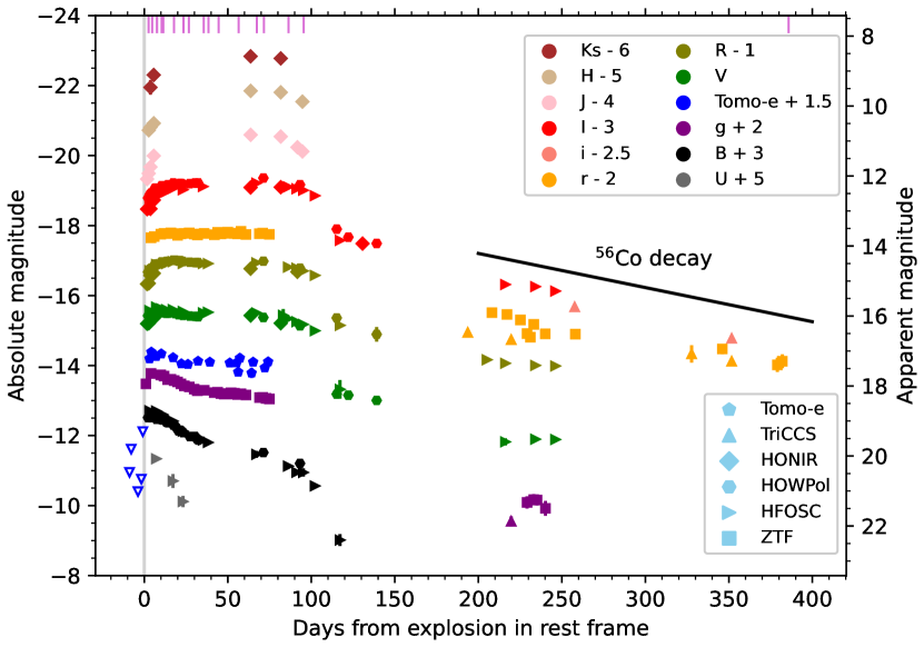
Figure 1: Light curves of SN 2021gmj in the optical ($U,B,g,$Tomo-e$,V,R,r,i,I$) and NIR ($J,H,K_{s}$) bands. The inverse open triangles represent the upper limits. The gray vertical line shows the inferred explosion date (see Section 4.3). The epochs of the spectroscopic observations are indicated with magenta lines on the upper x-axis. The black solid line shows the slope of the ⁵⁶Co decay.

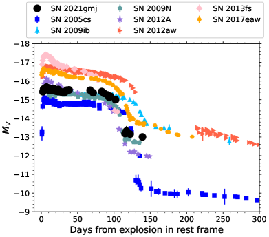
Figure 2: V-band light curves of SN 2021gmj and other Type IIP SNe: SN 2005cs (Tsvetkov et al. 2006; Pastorello et al. 2006, 2009), SN 2009ib (Takáts et al. 2015), SN 2009N (Takáts et al. 2014), SN 2012A (Tomasella et al. 2013), SN 2012aw (Fraser et al. 2012), SN 2013fs (Valenti et al. 2016; Bullivant et al. 2018) and SN 2017eaw (Tsvetkov et al. 2018). We obtained the data of the other SNe from the Open Supernova Catalog (https://github.com/astrocatalogs/supernovae; Guillochon et al. 2017).

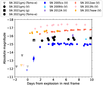
Figure 3: Early light curves of SN 2021gmj and other Type IIP SNe: SN 2005cs (Tsvetkov et al. 2006; Pastorello et al. 2006, 2009), SN 2009ib (Takáts et al. 2015), SN 2012A (Tomasella et al. 2013), SN 2012aw (Fraser et al. 2012), SN 2013fs (Valenti et al. 2016; Bullivant et al. 2018) and SN 2017eaw (Tsvetkov et al. 2018). The Tomo-e, $V$-, and $g$-band data are plotted for SN 2021gmj, while the $V$-band data are plotted for the other SNe. The inverse open triangles represent the upper limits. The gray inverse open triangle and filled circle show the last non-detection and first detection for SN 2021gmj, respectively (Valenti et al. 2021). We obtained the data of the other SNe from the Open Supernova Catalog (Guillochon et al., 2017).

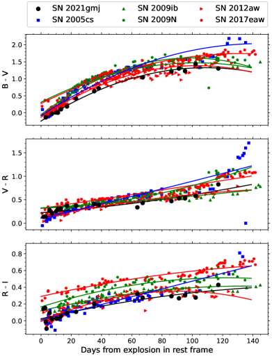
Figure 4: Color evolution of SN 2021gmj compared with other Type IIP SNe: the sub-luminous SN 2005cs (Tsvetkov et al. 2006; Pastorello et al. 2006, 2009), the intermediate-luminosity SNe 2009ib (Takáts et al. 2015), 2009N (Takáts et al. 2014), and the normal SNe 2012aw (Fraser et al. 2012), 2017eaw (Tsvetkov et al. 2018). The data of the other SNe were obtained from the Open Supernova Catalog. Red, green, and blue lines show the results of second order polynomial fitting for normal, intermediate-luminosity, and sub-luminous SNe, respectively.

Figure 1 shows the multi-band light curves of SN 2021gmj. In addition to our data, we obtained $g$- and $r$-band data from Zwicky Transient Facility (ZTF; Bellm et al. 2019) taken through the Automatic Learning for the Rapid Classification of Events (ALeRCE; Förster et al. 2021). We estimate the explosion date of SN 2021gmj as $t_{0}$ = 59292.321 MJD from a comparison of the Tomo-e- and $r$-band light curves with light curve models of Moriya et al. (2023) (see Section 4.3). For the other objects compared in following figures, we adopt the explosion time estimated in each object’s literature reference: they are typically estimated by the last non-detection and discovery dates and/or by analytic fitting of the rising part of the light curves.

SN 2021gmj reaches its brightness peak in optical bands very quickly (4-6 days) after the explosion. The absolute peak magnitudes of SN 2021gmj in the $V$ and $R$ bands are $\sim-15.5$ mag and $\sim-15.9$ mag, respectively, at $\sim 7$ days after the explosion. During the plateau phase, the Tomo-e, $V$-, $R$-, $r$- and $I$-band magnitudes are roughly constant, the $J$-, $H$- and $K_{s}$-band magnitudes slightly increase for $\sim 70$ days, and the $B$- and $g$-band magnitudes decline steadily. The plateau length of SN 2021gmj from the peak measured in the $V$ band is about 100 days, which is consistent with a typical plateau length of Type II SNe ($\sim 80$-120 days; Valenti et al. 2016). Type II SNe have a diversity in the plateau absolute magnitude ($-18\lesssim M_{V,\rm peak}\lesssim-14$) with a typical value of $\sim-16.7$ mag (Anderson et al. 2014; Valenti et al. 2016). The plateau absolute magnitude of SN 2021gmj (about $-15.5$ mag in the $V$ band) indicates the nature of intermediate-luminosity. In this paper, we define SNe with $-16\lesssim M_{V,\rm peak}\lesssim-15$ as intermediate-luminosity SNe, and SNe fainter than intermediate-luminosity SNe as sub-luminous SNe. Even if we consider the maximum extinction of $A_{V}\sim 0.3$ mag, the absolute magnitude of SN 2021gmj still falls in the intermediate luminosity range.

We compare the light curves of SN 2021gmj with those of other Type IIP SNe in Figure 2. The comparison SNe are the sub-luminous SN 2005cs (Tsvetkov et al. 2006; Pastorello et al. 2006; Pastorello et al. 2009), the normal SNe 2012aw (Fraser et al. 2012), 2013fs (Valenti et al. 2016; Bullivant et al. 2018), and 2017eaw (Tsvetkov et al. 2018) and the intermediate-luminosity SNe 2009ib (Takáts et al. 2015), 2009N (Takáts et al. 2014), and 2012A (Tomasella et al. 2013). The plateau length of SN 2021gmj ($\sim 100$ days) is similar to those of SNe 2009N and 2012A, and shorter than those of SNe 2005cs, 2009ib, 2012aw, and 2017eaw. While there is not sufficient data of SN 2013fs after the plateau phase, the plateau length of SN 2021gmj is longer than that of SN 2013fs.

The brightness drop from the plateau to tail phases in SN 2021gmj is $\sim 2$ mag with a duration of $\sim 20$ days in the $V$ band. This brightness drop is smaller than that of SN 2005cs, while it is similar to those of the other objects. After this drop in luminosity, the light curve shows a linear decline powered by the radioactive decay of ⁵⁶Co to ⁵⁶Fe. In the tail phase, SN 2021gmj is brighter than SNe 2005cs and 2012A while fainter than SN 2009ib. The luminosity in the tail phase of SN 2021gmj is similar to that of SN 2009N. We estimate the ⁵⁶Ni mass of SN 2021gmj from the luminosity in the tail phase in Section 4.1.

The early-phase light curves of SN 2021gmj and other Type IIP SNe are shown in Figure 3. For the other Type IIP SNe shown in the plot, we adopt the explosion date estimated in each object’s literature reference. Although there is no data during the rising part of SN 2021gmj, our observations combined with the ZTF data show that the duration of the rising part in SN 2021gmj resembles those of the other SNe.

The $B-V$, $V-R$ and $R-I$ color evolutions of SN 2021gmj are shown in Figure 4. The colors are compared to those of the sub-luminous SN, the intermediate-luminosity SNe and the normal SNe that are used for the photometric comparison in Figure 2. The solid curves show the fitting by the second order polynomial. The overall color evolutions of SN 2021gmj are within the range of other Type IIP SNe.

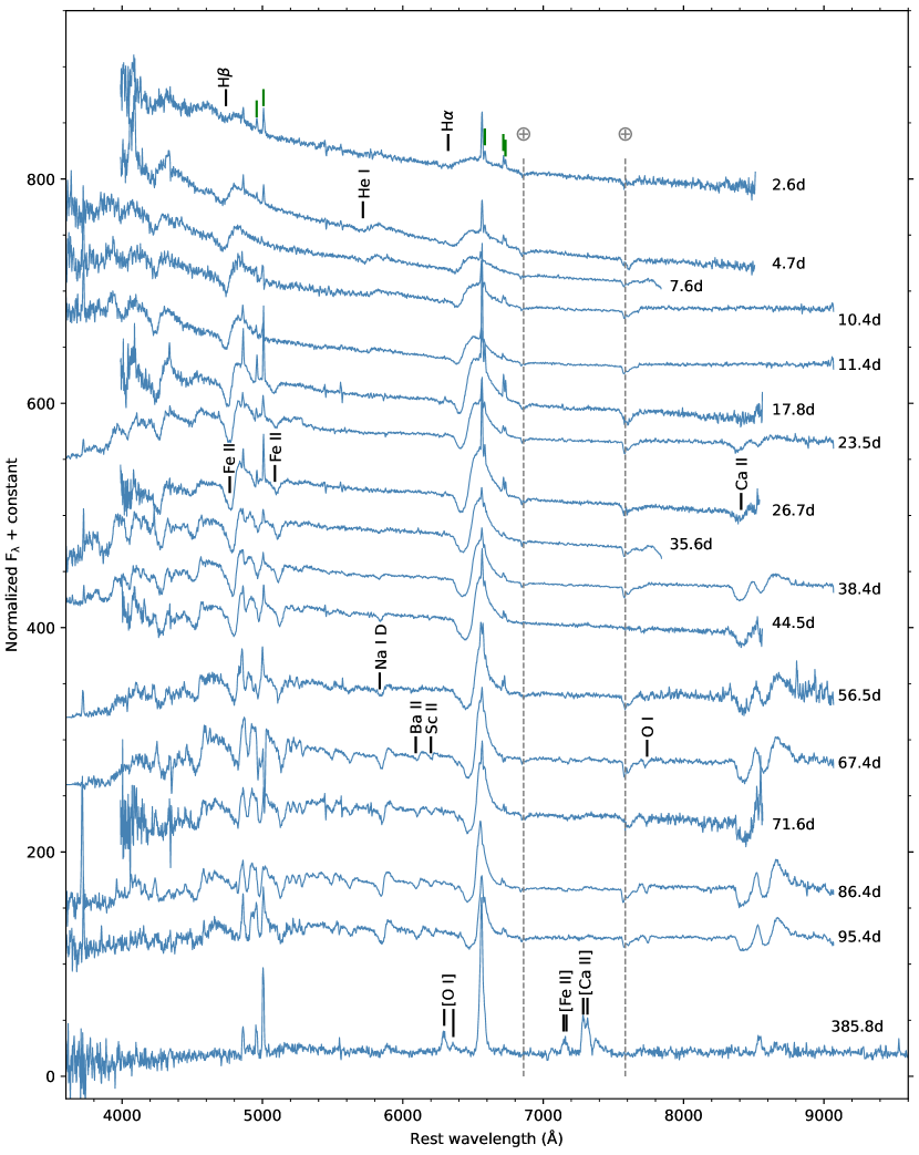
Figure 5: Spectral evolution of SN 2021gmj from 2.6 days to 385.8 days after the explosion. The green lines represent [O III] $\rm\lambda$4959,5007, [N II] $\rm\lambda$6584 and [S II] $\rm\lambda$6716,6731 originating from the nearby H II region. The narrow Balmer lines are also due to the contamination from the nearby H II region.

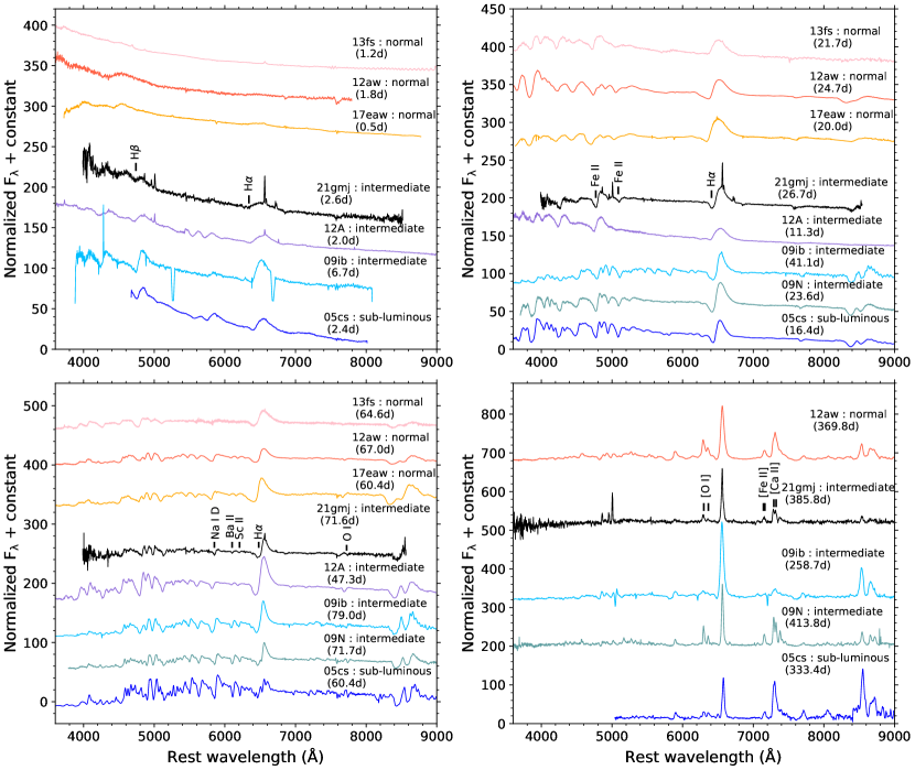
Figure 6: Spectra of SN 2021gmj from 2.6 to 385.8 days after the explosion, compared with the sub-luminous SN 2005cs (Tsvetkov et al. 2006; Pastorello et al. 2006, 2009), the intermediate-luminosity SNe 2009ib (Takáts et al. 2015), 2009N (Takáts et al. 2014) and 2012A (Tomasella et al. 2013), and the normal SNe 2012aw (Fraser et al. 2012), 2013fs (Valenti et al. 2016; Bullivant et al. 2018) and 2017eaw (Szalai et al. 2019; Van Dyk et al. 2019). We obtained the spectra of these Type IIP SNe from the Weizmann Interactive Supernova Data Repository (WISeREP; https://www.wiserep.org/; Yaron & Gal-Yam 2012).

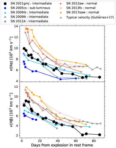
Figure 7: Velocity evolution of H$\rm\alpha$ and H$\rm\beta$ lines in SN 2021gmj compared with those of other Type IIP SNe. The gray lines are the results of Gutiérrez et al. (2017), that are the typical velocities for Type II SNe.

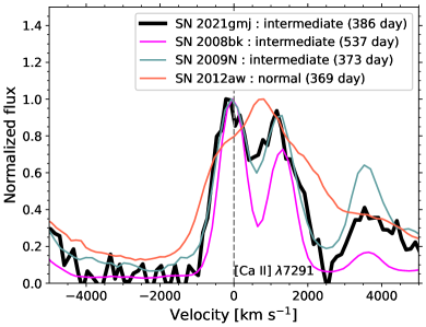
Figure 8: Line profiles of the [Ca II] $\lambda$7291,7324 lines in the nebular spectrum of SN 2021gmj ($R\sim 360$) compared with those of SNe 2008bk ($R\sim 730$), 2009N ($R\sim 520$), and 2012aw ($R\sim 460$). The [Ca II] lines are doublet, and the velocity is measured with respect to the rest wavelength of the bluer feature. We obtained the data from WISeREP.

3.2 Spectral evolution

The time series of the spectra of SN 2021gmj is presented in Figure 5. Overall, the spectra of SN 2021gmj show similar temporal evolution to other Type IIP SNe. As in other Type IIP SNe, the early spectra (< 5 days) are characterized by broad Balmer and He I $\rm\lambda$5876 lines superposed on a blue continuum. The H absorption lines generally get stronger as time goes by while the He I line disappears after 17.8 days after the explosion. The metal lines such as Fe II $\rm\lambda$4924, 5169, and Ca II IR triplet start to become prominent on 26.7 days after the explosion. In the latter half of the plateau phase (from day 56.5 to 95.4), the metal lines become stronger and the lines of Na I D $\rm\lambda$5889, 5895 and O I $\rm\lambda$7774 are visible. The Ba II $\rm\lambda$6142 and Sc II $\rm\lambda$6247 lines, as also seen in other SNe at similar epochs (Pastorello et al. 2004; Spiro et al. 2014; Gutiérrez et al. 2017; Pearson et al. 2023), are also visible. In the last spectrum in the nebular phase, several typical emission lines are detected such as [O I] $\rm\lambda$6300, 6364, [Ca II] $\rm\lambda$7291, 7324, and [Fe II] $\rm\lambda$7155, 7172.

In Figure 6, we compare the spectra of SN 2021gmj with those of the sub-luminous SN 2005cs, the intermediate-luminosity SNe 2009ib, 2009N, and 2012A, and the normal SNe 2012aw, 2013fs, and 2017eaw. Overall, the spectra of SN 2021gmj have a similarity to those of the intermediate-luminosity SNe and sub-luminous SNe rather than those of the normal SNe. In the earliest phase ($<$ 5 days, left upper panel of Figure 6), the spectrum of SN 2021gmj shows more structure than the normal SNe, and it is similar to those of the intermediate-luminosity and sub-luminous SNe.

During the plateau phase (right upper and left lower panels of Figure 6), the absorption features in SN 2021gmj are narrower than those in normal SNe, and similar to those in intermediate-luminosity and sub-luminous SNe. We estimate the velocities of H$\rm\alpha$ and H$\rm\beta$ lines by measuring their absorption minima after smoothing the spectra. The derived velocity evolution is shown in Figure 7 as compared with those of other Type IIP SNe. SN 2021gmj shows higher velocities than the sub-luminous SN 2005cs, while SN 2021gmj shows lower velocities compared to the normal SNe 2012aw, 2013fs, and 2017eaw. The velocities of SN 2021gmj are indeed similar to those of the intermediate-luminosity SNe 2009ib, 2009N, and 2012A.

A statistical study about ejecta expansion velocities for Type II SNe (Gutiérrez et al. 2017) shows that the range in ejecta expansion velocities is from $\sim 1,500~{}\rm km~{}s^{-1}$ to $\sim 9,600~{}\rm km~{}s^{-1}$ at 50 days after explosion with a median H$\rm\alpha$ value of 7,300 $\rm km~{}s^{-1}$. The H$\rm\alpha$ velocity of SN 2021gmj at 50 days after explosion is $\sim 5,300~{}\rm km~{}s^{-1}$, indicating SN 2021gmj is a low-velocity SN.

The low velocities of SN 2021gmj persist in the nebular phase (right lower panel of Figure 6). We compare the line profile of [Ca II] $\lambda$7291,7324 with those of the intermediate-luminosity SNe 2008bk, 2009N, and normal SN 2012aw in Figure 8. The line width of SN 2021gmj is consistent with the spectral resolution ($R\sim 360$), indicating that the velocity of SN 2021gmj is lower than $\sim 1,000~{}\rm km~{}s^{-1}$. SN 2021gmj clearly shows a narrower line profile than that of the normal SN 2012aw. The velocity of SN 2021gmj in the nebular phase is consistent with those of the intermediate-luminosity SNe 2008bk and 2009N.

In summary, the spectral properties of SN 2021gmj are quite similar to those of the intermediate-luminosity SNe 2009ib, 2009N, and 2012A. This indicates that SN 2021gmj belongs to a population between normal SNe and sub-luminous SNe in terms of spectroscopic properties.

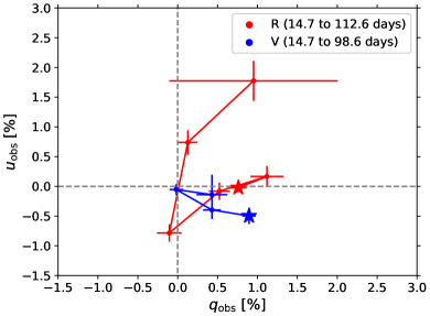
Figure 9: The observed Stokes parameters in the $q-u$ plane. The first epoch in both bands is 14.7 days after the explosion. The final epoch in $V,R$ bands is 98.6, 112.6 days, respectively. The stars represent the values in the first epoch.

3.3 Polarimetric evolution

We present imaging polarimetry of SN 2021gmj obtained over six epochs from $\sim 14$ to 112 days after the explosion. The observed Stokes parameters ($q_{\rm obs}$, $u_{\rm obs}$) in the $V$ and $R$ bands are shown in Figure 9. During the plateau phase until $105.4\pm 1.4$ days after explosion, the Stokes parameters are clustered around a point ($q\sim 0.5$ % and $u\sim-0.2$ %) in the $q-u$ plane, and they do not significantly vary during the plateau phase. SN 2021gmj then started showing a deviation from this point in the $q-u$ plane at the beginning of the tail phase ($2.0\pm 0.7$ days after the end of the plateau phase).

In addition to the intrinsic SN polarization, the SN light would also be polarized by non-spherical dust grains in the interstellar medium along the line of sight. This is called interstellar polarization (ISP). In order to investigate the intrinsic property of the SN polarization, it is necessary to remove the ISP component. For an accurate estimate of ISP, one must know the properties of dust grain along the line of sight within the host galaxy, which is usually difficult to obtain. Although many methods have been suggested to derive ISP (Trammell et al. 1993; Tran et al. 1997; Wang et al. 2001), each method involves some uncertainties (Wang & Wheeler 2008).

Here we give only a conservative estimate of the ISP and intrinsic SN polarization. The degree of the ISP is observationally related to the degree of the interstellar extinction ($p_{\rm ISP}\lesssim 9\times E(B-V)$ %, Serkowski et al., 1975). Non-detection of significant Na I D absorption lines in our spectra suggests an upper limit of the equivalent width of Na I D absorption lines is 0.7496 Å. This corresponds to $E(B-V)<0.1$ by using the empirical relation by Poznanski et al. (2012). This gives an upper limit of the ISP $p_{\rm ISP}\lesssim 0.9$ %. Thus, the obtained polarization degree in the plateau phase can be entirely caused by the ISP. This implies that H-rich envelope of SN 2021gmj is not strongly deviated from spherical symmetry. In general, Type IIP SNe show a low degree of the intrinsic polarization at early phases and show a rise to $\sim 1$ % degree at certain points during the plateau phase (e.g., Leonard et al. 2001; Chornock et al. 2010; Kumar et al. 2016; Nagao et al. 2023; Nagao et al. 2024). The observed properties of SN 2021gmj are consistent with this picture, although it is difficult to quantitatively estimate the degree of the intrinsic polarization due to the uncertainty in the ISP.

4 Discussion

4.1 Bolometric light curve

We derive the bolometric luminosity of SN 2021gmj by integrating the $U$-, $B$-, $V$-, $R$- and $I$-band photometry. For each observational epoch with more than 3 band data, we derived the fluxes at the effective wavelengths to specify the spectral energy distribution (SED) for each epoch. Then, we performed a blackbody fitting to the SED and derived the best-fit temperature and radius. Finally, the bolometric luminosity was derived by integrating the best-fit blackbody function as shown in Figure 10.

In Type IIP SNe, the luminosity at the tail phase is mainly powered by the radioactive decay of ⁵⁶Co. Therefore, the bolometric luminosity at the tail phase is a good indicator of the amount of ⁵⁶Ni  in the SN ejecta. This luminosity can be described as follows:

$$L_{\rm decay}(t)=(6.45\times 10^{43}e^{-t/\tau_{\rm Ni}}~{}+~{}1.45\times 10^{43}e^{-t/\tau_{\rm Co}})\left(\frac{M_{\rm Ni}}{M_{\odot}}\right)~{}\rm erg~{}s^{-1}~{},$$ (1)

where $t$ is time in days (Nadyozhin 1994). $\tau_{\rm Ni}$ and $\tau_{\rm Co}$ are the lifetime of ⁵⁶Ni  and ⁵⁶Co  in days, respectively. From this equation and the tail phase of the bolometric light curve of SN 2021gmj, the ⁵⁶Ni mass for SN 2021gmj is estimated to be $0.022\pm 0.006~{}\rm M_{\odot}$ (Figure 10).

The ⁵⁶Ni mass derived for SN 2021gmj is smaller than those of the normal SN 2012aw: $M(^{56}{\rm Ni})=0.05~{}\rm M_{\odot}$ (Nagy & Vinkó 2016), the normal SN 2017eaw: $M(^{56}{\rm Ni})=0.046~{}\rm M_{\odot}$ (Szalai et al. 2019), and the intermediate-luminosity SN 2009ib: $M(^{56}{\rm Ni})=0.046\pm 0.015~{}\rm M_{\odot}$ (Takáts et al. 2015). On the other hand, the ⁵⁶Ni mass of SN 2021gmj is larger than those of the sub-luminous SN 2005cs: $M(^{56}{\rm Ni})\sim 0.003~{}\rm M_{\odot}$ (Pastorello et al. 2009) and the intermediate-luminosity SN 2012A: $M(^{56}{\rm Ni})=0.011\pm 0.004~{}\rm M_{\odot}$ (Tomasella et al. 2013). The ⁵⁶Ni mass in SN 2021gmj is the most similar to that in the intermediate-luminosity SN 2009N: $M(^{56}{\rm Ni})=0.020\pm 0.004~{}\rm M_{\odot}$ (Takáts et al. 2014).

The ⁵⁶Ni mass in SN 2021gmj can also be compared with the results of statistical studies of Type II SNe. For instance, Müller et al. (2017) investigated the observed distribution of ⁵⁶Ni mass for 38 Type II SNe, showing a median and mean values of 0.031 and 0.046 $\rm M_{\odot}$, respectively. Anderson (2019) estimated a median ⁵⁶Ni mass for 115 Type II SNe to be 0.032 $\rm M_{\odot}$. Rodríguez et al. (2021) investigated the ⁵⁶Ni mass distribution for 110 Type II SNe with the average of $0.040\pm 0.005~{}\rm M_{\odot}$. More recently, Martinez et al. (2022) determined a median ⁵⁶Ni mass of 0.036 $\rm M_{\odot}$ for 17 Type II SNe, that have the ⁵⁶Ni mass distribution between 0.006 and 0.069 $\rm M_{\odot}$.

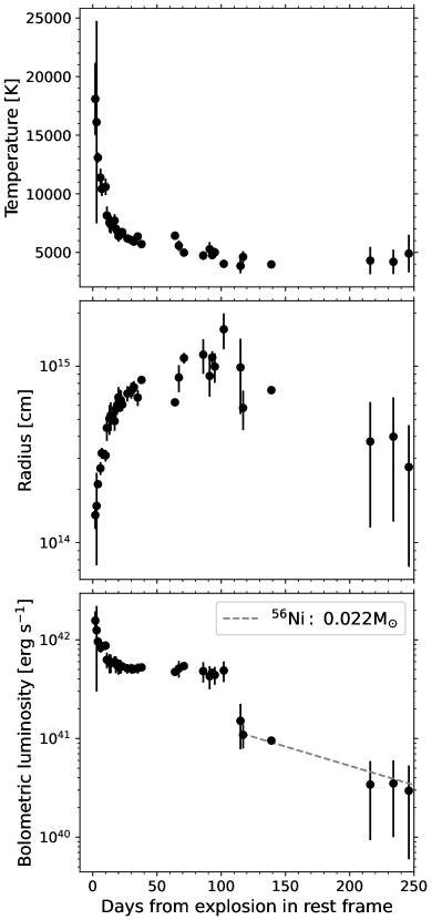
Figure 10: Blackbody evolutions of temperature (top), radius (middle), and bolometric luminosity (bottom) of SN 2021gmj. The gray dashed line in the bottom figure represents the decay luminosity from the $\rm{}^{56}Co$ decay (0.022 $\rm M_{\odot}$).

4.2 Progenitor mass

Spectroscopic observations of SNe at nebular phase provide useful information on the nucleosynthesis in SN explosions and their progenitors. As SN ejecta expands, their density decreases, and the inner parts are exposed. When the inner core becomes optically thin, the observed spectrum should be dominated by emission lines. In particular, the ratio of [O I] $\lambda$6300, 6364 and [Ca II] $\lambda$7291, 7324 lines is used as an indicator of progenitor mass. The [O I]/[Ca II] ratio is correlated with the progenitor oxygen mass, which is dependent on the progenitor mass (Fransson & Chevalier 1989; Maeda et al. 2007; Jerkstrand et al. 2015; Kuncarayakti et al. 2015; Jerkstrand 2017; Fang et al. 2022; Fang & Maeda 2023).

In the nebular spectrum of SN 2021gmj at 385.8 days after the explosion, we measured the line ratio of [O I]/[Ca II] to be 0.60 by fitting the [O I] and [Ca II] lines with double Gaussian functions. In order to infer the progenitor mass, we compared the line ratio with those of other Type IIP SNe with good constraints to the progenitor’s zero-age main-sequence (ZAMS) mass from their pre-explosion images: SN 1999em (Kuncarayakti et al. 2015; Smartt et al. 2003, 2009), SN 2004dj (Chugai et al. 2005; Maíz-Apellániz et al. 2004; Wang et al. 2005; Smartt et al. 2009), SN 2004et (Kuncarayakti et al. 2015; Smartt et al. 2009), SN 2005cs (Maund et al. 2005; Li et al. 2006; Pastorello et al. 2009; Smartt et al. 2009), SN 2007aa (Smartt et al. 2009), SN 2008bk (Maund et al. 2014), SN 2009N (Smartt 2015), SN 2009ib (Takáts et al. 2015; Smartt 2015), SN 2012A (Tomasella et al. 2013; Smartt 2015), and SN 2012aw (Fraser et al. 2012; Smartt 2015). The line ratios of these SNe are also measured by fitting double Gaussian to the lines. As shown in Figure 11, the [O I]/[Ca II] ratio shows a weak linear correlation with the progenitor mass. From this correlation, the progenitor mass of SN 2021gmj is estimated to be about 10 to 15 $\rm M_{\odot}$.

We also measure the [O I]/[Ca II] ratios in the spectral models for Type IIP SNe by Jerkstrand et al. (2014) (see Figure 11). Jerkstrand et al. (2014) generated models of nebular spectra from stellar evolution and explosion models using the spectral synthesis code described in Jerkstrand et al. (2011). These model spectra are calculated for the stars with 12, 15, 19 and 25 $\rm M_{\odot}$ initial mass. In Figure 12, we compare the [O I]/[Ca II] ratios of 12 and 15 $\rm M_{\odot}$ models at 400 days and 19 $\rm M_{\odot}$ model at 451 days with SN 2021gmj at 385.8 days, where the fluxes are scaled to match the [Ca II] $\lambda$7291, 7324 lines. From the comparison between the [O I]/[Ca II] ratios of the spectral models and SN 2021gmj, the progenitor mass of SN 2021gmj is likely to be about 12 $\rm M_{\odot}$, which is consistent with the mass estimated from the weak correlation between the [O I]/[Ca II] ratios and the progenitor mass of the other Type IIP SNe. The 12 $\rm M_{\odot}$ model also gives the best match with the SN spectrum from the similarities of [O I], [Fe II] and H$\alpha$ lines.

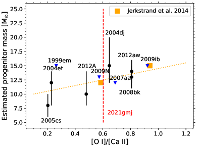
Figure 11: [O I]/[Ca II] ratio of SN 2021gmj and Type IIP SNe whose progenitor masses were estimated from the pre-explosion image analysis: SN 1999em (Kuncarayakti et al. 2015; Smartt et al. 2003, 2009), SN 2004dj (Chugai et al. 2005; Maíz-Apellániz et al. 2004; Wang et al. 2005; Smartt et al. 2009), SN 2004et (Kuncarayakti et al. 2015; Smartt et al. 2009), SN 2005cs (Maund et al. 2005; Li et al. 2006; Pastorello et al. 2009; Smartt et al. 2009), SN 2007aa (Smartt et al. 2009), SN 2008bk (Maund et al. 2014), SN 2009N (Smartt 2015), SN 2009ib (Takáts et al. 2015; Smartt 2015), SN 2012A (Tomasella et al. 2013; Smartt 2015), and SN 2012aw (Fraser et al. 2012; Smartt 2015). The object whose progenitor is detected in its pre-explosion image is represented in black dot while the object whose progenitor is not detected is represented in blue inverse triangle as an upper limit. The red dashed line represents the [O I]/[Ca II] ratio of SN 2021gmj. The orange square dots show the relation between the progenitor mass and [O I]/[Ca II] ratio of spectral models for Type IIP SNe (Jerkstrand et al. 2014).

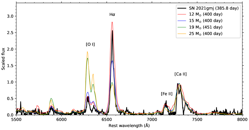
Figure 12: Comparison of the nebular spectrum of SN 2021gmj with the spectral models of Jerkstrand et al. (2014). Spectra are scaled to match the [Ca II] $\lambda$7291,7324 flux. The flux of narrow H$\rm\alpha$ from the host galaxy is subtracted from the observed flux assuming the flux ratio H$\rm\alpha$/H$\rm\beta$ to be 3:1.

4.3 Explosion and circumstellar material properties

The rising part of light curves of Type IIP SNe can be used as a probe of circumstellar material (CSM) (e.g., Moriya et al. 2011, 2017, 2018; Morozova et al. 2017, 2018; Förster et al. 2018). In order to estimate explosion and CSM properties, we compared the Tomo-e and $r$-band light curves with the light curve models by Moriya et al. (2023). In these models, red supergiant (RSG) models in Sukhbold et al. (2016) are adopted as the progenitors for Type IIP SNe. The confined CSM is attached on the surface of the progenitors. For the calculations of the light curve models, the radiation hydrodynamics code $\rm STELLA$ (Blinnikov et al. 1998, 2000, 2006) is used. To initiate the explosion, thermal energy is injected just above a mass cut to trigger the explosion.

The mass cut of the progenitor is set at 1.4 $\rm M_{\odot}$. The density structure of the CSM is assumed as in Moriya et al. (2017, 2018),

$$\rho_{\rm CSM}\left(r\right)=\frac{\dot{M}}{4\pi v_{\rm wind}\left(r\right)r^{2}}~{},$$ (2)

where $r$ is the radius from the center of a progenitor, $\dot{M}$ is the mass-loss rate of a progenitor, and $v_{\rm wind}$ is the wind velocity. The wind velocity is expressed as a function of radius:

$$v_{\rm wind}(r)=v_{0}+(v_{\infty}-v_{0})\left(1-\frac{R_{0}}{r}\right)^{\beta}~{},$$ (3)

where $v_{0}$ is an initial wind velocity at the surface of a progenitor, $v_{\infty}$ is a terminal wind velocity, $R_{0}$ is a progenitor radius, and $\beta$ is a wind structure parameter. Here, $v_{0}$ is the value that smoothly connects the CSM to the progenitor surface, and $v_{\infty}$ is assumed to be $\rm 10~{}km~{}s^{-1}$ (Moriya et al., 2023). The parameters in the model sets are the ZAMS mass of the progenitor ($M_{\rm ZAMS}$), the ⁵⁶Ni mass ($M_{\rm Ni}$), the wind parameter ($\beta$), the CSM radius ($R_{\rm CSM}$), the explosion energy ($E$), and the mass-loss rate ($\dot{M}$).

Since the explosion energy and the mass-loss rate mainly affect the rising part of light curves, we fix the other parameters as follows: $M_{\rm ZAMS}=12~{}\rm M_{\odot}$, $M_{\rm Ni}=0.02~{}\rm M_{\odot}$, $\beta=2$, and $R_{\rm CSM}=4\times 10^{14}~{}\rm cm$. As RSGs are known to accelerate the wind slowly (e.g., Schroeder (1985)), we fix $\beta$ to be 2. Note that it does not affect the early light curves much. We assume the breakout time when a photosphere reaches to the outer edge of the CSM is 20 days after explosion based on the observed light curve (Figure 1). From this assumption, we fix $R_{\rm CSM}=4\times 10^{14}$ cm here. It also means that the CSM affects the light curves only until 20 days after explosion, thus the explosion energy can be determined by the light curves after this epoch. We then vary the explosion energy (0.2, 0.3, 0.5, 1.0, and 1.5$\times~{}10^{51}\rm erg$) and the mass-loss rate ($10^{-5.0},~{}10^{-4.5},~{}10^{-4.0},~{}10^{-3.5},~{}10^{-3.0},~{}10^{-2.5},$ and $10^{-2.0}~{}\rm M_{\odot}~{}yr^{-1}$). The light curve models with 0.5, 1.0, and 1.5$\times~{}10^{51}\rm erg$ of the explosion energy are calculated in Moriya et al. (2023). We additionally calculated the light curves for these low-energy models (0.2 and 0.3 $\times~{}10^{51}\rm erg$) using $\rm STELLA$ code in the same way as Moriya et al. (2023). We compare the Tomo-e and $r$-band light curves of the early phase ($\leq$ 40 days after the explosion) with the available light curve models from Moriya et al. (2023) and the newly calculated low-energy models. In the comparison, the explosion date is also parameterized with a range between the last non-detection date and the discovery date.

First, we estimate the explosion energy by comparing the light curve models with various explosion energy for a fixed mass-loss rate $10^{-5.0}~{}\rm M_{\odot}~{}yr^{-1}$ (Figure 13). For the estimate of the explosion energy, we use the plateau luminosity from the breakout time ($\sim 20$ days) to 40 days after the explosion. This is because: (a) plateau luminosity is mainly determined by explosion energy when a progenitor mass is fixed (e.g., Kasen & Woosley 2009); (b) the effect of CSM in light curves is not significant after the breakout time. Thus, this comparison is used only to estimate the explosion energy to reproduce the plateau luminosity. We find the model with $E=0.3\times 10^{51}$ erg best matches to the light curves in both bands.

Then, with this estimated explosion energy, we estimate the mass-loss rate by changing the mass-loss rate (Figure 14). We find a higher mass-loss rate can reproduce the rising parts of the light curves better. As shown in Figure 14, the model with a high mass-loss rate ($\dot{M}=10^{-3}~{}\rm M_{\odot}~{}yr^{-1}$) reproduces the fast rise of the light curves as compared with the model with a normal mass-loss rate ($\dot{M}\lesssim 10^{-5}~{}\rm M_{\odot}~{}yr^{-1}$; Smith 2014), indicating that dense CSM exists around the progenitor of SN 2021gmj just before the explosion. This finding is consistent with those suggested for normal SNe (e.g., Valenti et al. 2016; Morozova et al. 2017, 2018; Förster et al. 2018).

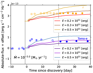
Figure 13: Comparison of the observed light curves with the model light curves with $E=0.2,0.3,$ and $0.5\times 10^{51}$ erg. Other parameters of the models are fixed: $M_{\rm ZAMS}=12~{}\rm M_{\odot}$, $M_{\rm Ni}=0.02~{}\rm M_{\odot}$, $\beta=2$, $R_{\rm CSM}=4\times 10^{14}~{}\rm cm$ and $\dot{M}=10^{-5}~{}\rm M_{\odot}~{}yr^{-1}$. The gray solid line is the estimated explosion date. The gray dashed line is the breakout time (20 days). The model light curve with $E=0.5\times 10^{51}$ erg of the explosion energy comes from Moriya et al. (2023). The model light curves with $E=0.2$ and $0.3\times 10^{51}$ erg of the explosion energy are calculated using STELLA code in the same way as Moriya et al. (2023).

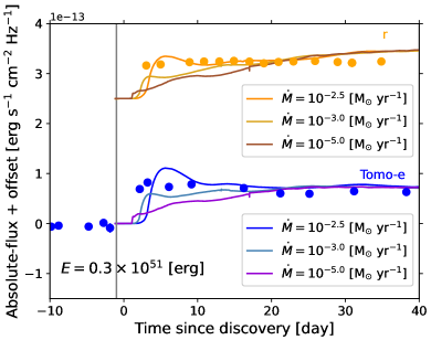
Figure 14: Comparison of the observed light curves with the model light curves with $\dot{M}=10^{-2.5},10^{-3},$ and $10^{-5}~{}\rm M_{\odot}~{}yr^{-1}$. Other parameters of the models are fixed: $M_{\rm ZAMS}=12~{}\rm M_{\odot}$, $M_{\rm Ni}=0.02~{}\rm M_{\odot}$, $\beta=2$, $R_{\rm CSM}=4\times 10^{14}~{}\rm cm$ and $E=0.3\times 10^{51}~{}\rm erg$. The gray vertical line is the estimated explosion date.

4.4 Early spectral features

Emission features in early spectra also provide clues to the properties of CSM. The spectrum of SN 2021gmj at 2.6 days exhibits a broad feature spreading from $\sim 4500$ Å  to $\sim 4750$ Å (Figure 15). This broad feature around 4600 Å is referred to as a "ledge" feature (Andrews et al. 2019; Soumagnac et al. 2020; Hosseinzadeh et al. 2022; Pearson et al. 2023), which is often seen in the early spectra of Type IIP SNe. This feature is also seen in the early spectra of some sub-luminous SNe: SN 2005cs (Pastorello et al. 2006), SN 2010id (Gal-Yam et al. 2011), SN 2016bkv (Hosseinzadeh et al. 2018), and SN 2018lab (Pearson et al. 2023).

The origin of this ledge feature in early spectra of Type IIP SNe is explained with a blend of some ionized lines originating from their CSM (e.g., Hosseinzadeh et al. 2022; Teja et al. 2022; Pearson et al. 2023). We compare the first-epoch spectrum of SN 2021gmj with a spectrum of SN 2018lab at a similar epoch in Figure 15. There is a remarkable similarity in the overall spectral shapes of these objects. In the case of SN 2018lab, although this emission feature can be interpreted as high-velocity H$\rm\beta$, there is no indication of a high-velocity H$\rm\alpha$ emission at the same epoch. Thus, it is concluded that this feature is due to the several ionized lines from the CSM: He II, C III, N III and N V (Pearson et al. 2023). In the case of SN 2021gmj, there is also no indication of a high-velocity feature of H$\rm\alpha$ at the same epoch. Hence, we attribute these emission lines in SN 2021gmj to He II, C III, N III and N V lines originating from its CSM as in SN 2018lab. The fact that this feature disappeared in the spectrum at 4.7 days after the explosion supports this interpretation. This also implies the presence of a large amount of CSM around the progenitor of SN 2021gmj as suggested from the early light curves.

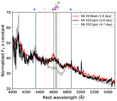
Figure 15: Comparison of the spectra of SN 2021gmj at 2.6 and 4.7 day with the spectrum of SN 2018lab at 1.9 day (Pearson et al. 2023). The rest wavelengths of the candidate lines are shown by vertical dashed lines.

4.5 Comparison with other Type IIP SNe

Here we compare the estimated mass-loss rates among Type II SNe and discuss the progenitor properties. Figure 16 shows the estimated mass-loss rate as a function of the peak absolute magnitude. Our result for SN 2021gmj (red) is compared with the results from other studies including large samples of Type II SNe. Förster et al. (2018) constrained progenitor mass-loss rates from $10^{-4}$ to $10^{-2}~{}\rm M_{\odot}~{}yr^{-1}$ using early part of light curves and multi-wavelength radiative transfer models. Subrayan et al. (2023) also estimated mass loss rate for ZTF Type II SNe to be $10^{-4}-$ $10^{-1}~{}\rm M_{\odot}~{}yr^{-1}$ using multi-wavelength radiative transfer models. Boian & Groh (2020) analyzed early-time spectra by comparing with the detailed spectral models. The estimated mass-loss rates vary from a few $10^{-4}$ to 1 $\rm M_{\odot}~{}yr^{-1}$. The results from the other individual studies are also plotted in Figure 16. Such individual studies mainly focus on normal-luminosity SNe. The estimated mass-loss rates are $\sim 10^{-3}-10^{-2}~{}\rm M_{\odot}~{}yr^{-1}$.

The number of studies for intermediate-luminosity or sub-luminous SNe is still small. The mass-loss rate for SN 2016bkv ($M_{V}\sim-16$) is estimated to be $\sim 6\times 10^{-4}-1.7\times 10^{-2}~{}\rm M_{\odot}~{}yr^{-1}$ by the analysis of early-time light curves and spectra (Nakaoka et al. 2018; Deckers et al. 2021). For SN 2018lab ($M_{V}\sim-15.1$), which is also one of the sub-luminous SNe, Pearson et al. (2023) estimated the mass-loss rate to be $\sim 5\times 10^{-3}~{}\rm M_{\odot}~{}yr^{-1}$ by analyzing early-time spectra. Our results on SN 2021gmj newly add an estimate of mass-loss rate in the lower-luminosity SN samples: $10^{-3}-10^{-2.5}~{}\rm M_{\odot}~{}yr^{-1}$ (Section 4.3). All of these studies so far suggest that, as in normal SNe, low-luminosity SNe also have higher mass-loss rates than typical mass-loss rate of RSGs. We infer that the progenitor of SN 2021gmj is a relatively low-mass RSG (Section 4.2). These results suggest a relatively low-mass SN progenitor can also experience the enhanced mass loss just before explosion, which gives a hint to understand the mechanism of the enhanced mass loss.

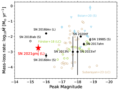
Figure 16: The estimated mass-loss rate and peak absolute magnitude relation for SN 2021gmj and other Type II SNe. The sample here includes previous statistical studies (Förster et al. 2018; Boian & Groh 2020; Subrayan et al. 2023) and individual studies: SN 1998S (Shivvers et al. 2015), SN 2013fs (Yaron et al. 2017; Moriya et al. 2017), SN 2016bkv (Nakaoka et al. 2018; Deckers et al. 2021), SN 2017ahn (Tartaglia et al. 2021), SN 2018lab (Pearson et al. 2023), SN 2020tlf (Jacobson-Galán et al. 2022), and SN 2023ixf (Bostroem et al. 2023; Grefenstette et al. 2023; Teja et al. 2023a). For the individual objects, peak absolute magnitude is taken from the Open Supernova Catalog. For the results by Subrayan et al. (2023), we show only the the objects with a good light curve coverage and a good model fit. The bands of peak absolute magnitude are following: $g$ (Förster et al., 2018; Subrayan et al., 2023), $r$ and $R$ (Boian & Groh 2020), $V$ (SN 1998S, 2013fs, 2016bkv, 2017ahn, 2018lab, 2020tlf, 2021gmj, and 2023ixf). Mass-loss rate is estimated by analyzing either light curves or spectra. (L) and (S) in the figures represent the methods to estimate of mass-loss rate: (L) is light curves, (S) is spectra. Open circles (triangles) are the estimated mass loss rate (upper limit) using only light curves or spectra while filled circles show the estimated mass loss rate using both light curves and spectra.

5 Conclusions

In this paper, we presented detailed photometric, spectroscopic and imaging polarimetric observations of the intermediate-luminosity Type IIP SN 2021gmj. The data were taken from a few days after the explosion to more than a year. The photometric observations of SN 2021gmj show that this SN lies at the luminosity range between sub-luminous and normal Type IIP SNe. The peak absolute $V$-band magnitude of SN 2021gmj is $-15.5$ mag, similar to those of intermediate-luminosity SNe 2009ib, 2009N and 2012A. The plateau length of SN 2021gmj is also similar to those of SN 2009N and 2012A.

The spectral evolution also indicates that SN 2021gmj is an intermediate-luminosity Type IIP SN. The spectra of SN 2021gmj have narrow line profiles that are seen in those of sub-luminous SNe and intermediate-luminosity SNe. We measure the velocities of H$\alpha$ and H$\beta$ lines and compared them with those of other Type IIP SNe. The ejecta velocity of SN 2021gmj is also between normal SNe and sub-luminous SNe.

Using the tail bolometric luminosity, the ⁵⁶Ni mass of SN 2021gmj is estimated to be about 0.022 $\rm M_{\odot}$. This is also intermediate between the normal SNe and sub-luminous SN 2005cs, and close to that of SN 2009N. Comparison of the nebular emission line ratio of [O I] $\lambda$6300,6364/[Ca II] $\lambda$7291,7324 with theoretical models (Jerkstrand et al. 2014) suggests that the ZAMS mass of SN 2021gmj is about 12 $\rm M_{\odot}$ which is a lower end of massive stars.

We estimate the properties of the explosion and the CSM by comparing the observed light curves with the light curve models from Moriya et al. (2023). We find that the explosion energy of $3\times 10^{50}~{}\rm erg$ gives a best fit to the plateau luminosity. The models with the mass-loss rate of $10^{-3}$ to $10^{-2.5}~{}\rm M_{\odot}~{}yr^{-1}$ can reproduce the fast rise of the light curve, suggesting that the dense CSM exists around the progenitor of SN 2021gmj before the explosion. In the spectra just after the explosion, a broad ledge feature around 4,600 Å is observed. This feature is likely caused by a blend of several highly-ionized lines from the CSM. It further supports the presence of the CSM around the progenitor of SN 2021gmj. From these properties of SN 2021gmj, we suggest that a relatively low-mass SN progenitor of intermediate-luminosity SNe can also experiences the enhanced mass loss just before the explosion, as suggested for normal Type IIP SNe.

Data Availability

The data used in this research will be shared on reasonable request to the corresponding author.

¹Astronomical Institute, Tohoku University, Sendai 980-8578, Japan
²Division for the Establishment of Frontier Sciences, Organization for Advanced Studies, Tohoku University, Sendai 980-8577, Japan
³Nishi-Harima Astronomical Observatory, Center for Astronomy, University of Hyogo, 407-2 Nishigaichi, Sayo-cho, Sayo, Hyogo 679-5313, Japan
⁴Department of Astronomy, Kyoto University, Kitashirakawa-Oiwake-cho, Sakyo-ku, Kyoto 606-8502, Japan
⁵Indian Institute of Astrophysics, Koramangala 2nd Block, Bangalore 560034, India
⁶Pondicherry University, Chinna Kalapet, Kalapet, Puducherry 605014, India
⁷Hiroshima Astrophysical Science Centre, Hiroshima University, 1-3-1 Kagamiyama, Higashi-Hiroshima, Hiroshima 739-8526, Japan
⁸Department of Physics, Graduate School of Advanced Science and Engineering, Hiroshima University, 1-3-1 Kagamiyama, Higashi-Hiroshima, Hiroshima 739-8526, Japan
⁹Department of Physics and Astronomy, University of Turku, FI-20014 Turku, Finland
¹⁰Aalto University Metsähovi Radio Observatory, Metsähovintie 114, 02540 Kylmälä, Finland
¹¹Aalto University Department of Electronics and Nanoengineering, P.O. BOX 15500, FI-00076 AALTO Finland
¹²National Astronomical Observatory of Japan, National Institutes of Natural Sciences, 2-21-1 Osawa, Mitaka, Tokyo 181-8588, Japan
¹³School of Physics and Astronomy, Faculty of Science, Monash University, Clayton, Victoria 3800, Australia
¹⁴Astronomical Science Program, Graduate Institute for Advanced Studies, SOKENDAI, 2-21-1 Osawa, Mitaka, Tokyo 181-8588, Japan
¹⁵Department of Physics, Faculty of Science and Engineering, Konan University, 8-9-1 Okamoto, Kobe, Hyogo 658-8501, Japan
¹⁶Kavli Institute for the Physics and Mathematics of the Universe (WPI), The University of Tokyo, 5-1-5 Kashiwanoha, Kashiwa, Chiba 277-8583, Japan
¹⁷Planetary Exploration Research Center, Chiba Institute of Technology, 2-17-1 Tsudanuma, Narashino, Chiba 275-0016, Japan
¹⁸Institute of Astronomy, Graduate School of Science, The University of Tokyo, 2-21-1 Osawa, Mitaka, Tokyo 181-0015, Japan
¹⁹Okayama Observatory, Kyoto University, 3037-5 Honjo, Kamogatacho, Asakuchi, Okayama 719-0232, Japan
²⁰Department of Multi-Disciplinary Sciences, Graduate School of Arts and Sciences, The University of Tokyo, 3-8-1 Komaba, Meguro, Tokyo 153-8902, Japan
²¹Kiso Observatory, Institute of Astronomy, Graduate School of Science, The University of Tokyo, 10762-30 Mitake, Kiso-machi, Kiso-gun, Nagano 397-0101, Japan
²²Okayama Branch Office, Subaru Telescope, NAOJ, NINS, Kamogata, Asakuchi, Okayama 719-0232, Japan
²³Japan Spaceguard Association, Bisei Spaceguard Center, 1716-3 Okura, Bisei, Ibara, Okayama 714-1411, Japan
²⁴UTokyo Organization for Planetary Space Science, The University of Tokyo, 7-3-1 Hongo, Bunkyo-ku, Tokyo 113-0033, Japan
²⁵Collaborative Research Organization for Space Science and Technology, The University of Tokyo, 7-3-1 Hongo, Bunkyo-ku, Tokyo 113-0033, Japan
²⁶Amanogawa Galaxy Astronomy Research Center (AGARC), Graduate School of Science and Engineering, Kagoshima University, 1-21-35 Korimoto, Kagoshima, Kagoshima 890-0065, Japan

Appendix A Data tables

Table 1: Optical photometry of SN 2021gmj

UT Date	MJD	Phasea	$U$	$B$	$g$	Tomo-e	$V$	$R$	$r$	$i$	$I$
(YYYY-MM-DD)		(days)	(mag)	(mag)	(mag)	(mag)	(mag)	(mag)	(mag)	(mag)	(mag)
2021-03-21	59294.57	1.25	-	15.98 (0.029)	-	-	16.05 (0.037)	15.79 (0.026)	-	-	15.66 (0.021)
2021-03-21	59294.75	1.43	-	-	-	-	16.28 (0.11)	16.13 (0.031)	-	-	15.98 (0.082)
2021-03-22	59295.48	2.16	-	-	-	15.79 (0.064)	-	-	-	-	-
2021-03-22	59295.50	2.18	-	15.79 (0.054)	-	-	16.26 (0.046)	16.11 (0.15)	-	-	15.95 (0.051)
2021-03-22	59295.60	2.28	-	15.97 (0.023)	-	-	15.98 (0.020)	15.71 (0.021)	-	-	15.56 (0.022)
2021-03-23	59296.46	3.14	-	15.98 (0.027)	-	-	15.96 (0.022)	15.68 (0.02)	-	-	15.52 (0.021)
2021-03-23	59296.54	3.22	-	-	-	15.60 (0.051)	-	-	-	-	-
2021-03-23	59296.54	3.22	-	-	-	-	-	15.89 (0.061)	-	-	15.97 (0.11)
2021-03-25	59298.52	5.21	-	-	-	-	16.12 (0.074)	15.83 (0.044)	-	-	15.72 (0.019)
2021-03-25	59298.68	5.37	-	15.95 (0.022)	-	-	15.89 (0.023)	15.56 (0.023)	-	-	15.38 (0.020)
2021-03-26	59299.43	6.11	-	-	-	15.72 (0.083)	-	-	-	-	-
2021-03-26	59299.50	6.18	15.17 (0.069)	15.79 (0.048)	-	-	15.80 (0.034)	15.75 (0.008)	-	-	15.54 (0.020)
2021-03-26	59299.60	6.28	-	16.03 (0.025)	-	-	15.93 (0.021)	15.56 (0.027)	-	-	15.38 (0.025)
2021-03-29	59302.49	9.17	-	-	-	15.65 (0.041)	-	-	-	-	-
2021-03-29	59302.50	9.18	-	15.88 (0.075)	-	-	15.85 (0.103)	15.58 (0.021)	-	-	15.54 (0.022)
2021-03-29	59302.67	9.35	-	16.04 (0.027)	-	-	15.96 (0.022)	15.50 (0.023)	-	-	15.31 (0.024)
2021-03-30	59303.45	10.13	-	16.05 (0.021)	-	-	15.97 (0.026)	15.53 (0.021)	-	-	15.36 (0.022)
2021-03-30	59303.50	10.18	-	15.90 (0.065)	-	-	15.88 (0.022)	15.56 (0.032)	-	-	15.52 (0.040)
2021-04-01	59305.48	12.16	-	16.11 (0.022)	-	-	15.98 (0.020)	15.49 (0.021)	-	-	15.31 (0.021)
2021-04-01	59305.50	12.18	-	16.00 (0.015)	-	-	15.88 (0.007)	15.55 (0.010)	-	-	15.48 (0.031)
2021-04-02	59306.52	13.20	-	16.13 (0.021)	-	-	15.98 (0.020)	15.48 (0.020)	-	-	15.28 (0.020)
2021-04-05	59309.50	16.18	15.81 (0.199)	16.08 (0.025)	-	-	15.88 (0.011)	15.49 (0.012)	-	-	15.39 (0.017)
2021-04-05	59309.57	16.25	-	-	-	15.75 (0.002)	-	-	-	-	-
2021-04-05	59309.66	16.34	-	16.19 (0.021)	-	-	15.96 (0.021)	15.45 (0.020)	-	-	15.23 (0.020)
2021-04-06	59310.74	17.42	-	16.22 (0.020)	-	-	15.99 (0.020)	15.45 (0.020)	-	-	15.26 (0.021)
2021-04-07	59311.72	18.40	-	16.28 (0.025)	-	-	15.97 (0.026)	15.46 (0.022)	-	-	15.26 (0.021)
2021-04-08	59312.76	19.44	-	16.36 (0.040)	-	-	16.02 (0.023)	15.48 (0.020)	-	-	15.26 (0.020)
2021-04-09	59313.78	20.46	-	16.34 (0.023)	-	-	16.01 (0.020)	15.46 (0.020)	-	-	15.24 (0.020)
2021-04-10	59314.51	21.20	-	-	-	15.93 (0.042)	-	-	-	-	-
2021-04-10	59314.69	21.37	-	16.37 (0.021)	-	-	16.02 (0.020)	15.48 (0.020)	-	-	15.25 (0.022)
2021-04-11	59315.50	22.18	16.39 (0.160)	16.37 (0.021)	-	-	15.93 (0.012)	15.54 (0.013)	-	-	15.42 (0.048)
2021-04-11	59315.55	22.23	-	16.41 (0.022)	-	-	16.04 (0.021)	15.49 (0.020)	-	-	15.27 (0.021)
2021-04-14	59318.45	25.13	-	-	-	15.94 (0.081)	-	-	-	-	-
2021-04-15	59319.56	26.24	-	16.52 (0.020)	-	-	16.06 (0.020)	15.51 (0.021)	-	-	15.25 (0.020)
2021-04-18	59322.70	29.38	-	16.52 (0.033)	-	-	16.07 (0.025)	15.52 (0.022)	-	-	15.23 (0.020)
2021-04-19	59323.68	30.36	-	16.58 (0.026)	-	-	16.07 (0.022)	15.52 (0.021)	-	-	15.24 (0.021)
2021-04-20	59324.50	31.18	-	-	-	15.86 (0.097)	-	-	-	-	-
2021-04-20	59324.58	31.26	-	16.62 (0.020)	-	-	16.08 (0.021)	15.52 (0.021)	-	-	15.23 (0.020)
2021-04-23	59327.50	34.18	-	16.62 (0.097)	-	-	15.97 (0.020)	15.55 (0.022)	-	-	15.33 (0.035)
2021-04-26	59330.50	37.18	-	16.69 (0.029)	-	-	15.95 (0.022)	15.55 (0.005)	-	-	-
2021-04-27	59331.57	38.25	-	-	-	15.88 (0.041)	-	-	-	-	-
2021-05-09	59343.53	50.21	-	-	-	15.91 (0.051)	-	-	-	-	-
2021-05-13	59347.58	54.26	-	-	-	15.90 (0.012)	-	-	-	-	-
2021-05-14	59348.53	55.21	-	-	-	16.17 (0.032)	-	-	-	-	-
2021-05-15	59349.54	56.22	-	-	-	15.77 (0.14)	-	-	-	-	-
2021-05-22	59356.57	63.25	-	-	-	16.19 (0.14)	-	-	-	-	-
2021-05-22	59356.58	63.26	-	-	-	-	16.04 (0.045)	15.69 (0.025)	-	-	15.36 (0.070)
2021-05-23	59357.49	64.17	-	-	-	15.88 (0.026)	-	-	-	-	-
2021-05-25	59359.50	66.18	-	17.03 (0.098)	-	-	15.97 (0.032)	15.53 (0.033)	-	-	15.24 (0.038)
2021-05-29	59363.63	70.31	-	16.98 (0.021)	-	-	16.1 (0.020)	15.48 (0.021)	-	-	15.09 (0.023)
2021-05-30	59364.48	71.16	-	-	-	16.04 (0.096)	-	-	-	-	-
2021-06-01	59366.47	73.15	-	-	-	15.87 (0.056)	-	-	-	-	-
2021-06-09	59374.48	81.16	-	-	-	-	16.26 (0.011)	-	-	-	15.35 (0.021)
2021-06-10	59375.50	82.18	-	-	-	-	16.04 (0.180)	-	-	-	-
2021-06-13	59378.50	85.18	-	17.37 (0.018)	-	-	16.13 (0.015)	15.65 (0.016)	-	-	15.34 (0.023)
2021-06-18	59383.50	90.18	-	17.54 (0.074)	-	-	16.22 (0.029)	15.68 (0.014)	-	-	15.40 (0.015)
2021-06-19	59384.52	91.20	-	-	-	-	-	15.78 (0.038)	-	-	-
2021-06-20	59385.55	92.23	-	17.29 (0.022)	-	-	16.34 (0.021)	15.68 (0.020)	-	-	15.28 (0.027)
2021-06-22	59387.50	94.18	-	17.55 (0.117)	-	-	16.30 (0.018)	15.76 (0.018)	-	-	15.44 (0.060)
2021-06-29	59394.50	101.18	-	17.93 (0.020)	-	-	16.48 (0.022)	15.89 (0.020)	-	-	15.60 (0.068)
2021-07-12	59407.54	114.22	-	18.38 (0.066)	-	-	18.29 (0.049)	17.10 (0.023)	-	-	16.55 (0.025)
2021-07-14	59409.50	116.18	-	19.48 (0.170)	-	-	-	17.31 (0.016)	-	-	16.87 (0.034)
2021-07-19	59414.51	121.19	-	-	-	-	18.32 (0.020)	-	-	-	16.78 (0.020)
2021-07-28	59423.49	130.17	-	-	-	-	-	-	-	-	16.96 (0.023)
2021-08-05	59431.46	138.15	-	18.53 (0.13)	-	-	18.47 (0.037)	17.57 (0.21)	-	-	16.96 (0.027)
2021-09-29	59486.82	193.50	-	-	-	-	-	-	18.52 (0.078)	-	-
2021-10-10	59497.50	204.18	-	-	-	-	-	18.30 (0.056)	-	-	-
2021-10-21	59508.50	215.18	-	-	-	-	19.65 (0.102)	18.40 (0.051)	-	-	18.13 (0.054)
2021-10-25	59512.80	219.48	-	-	19.94 (0.14)	-	-	-	18.73 (0.072)	-	-
2021-11-08	59526.50	233.18	-	-	-	-	19.58 (0.045)	18.46 (0.029)	-	-	18.19 (0.047)
2021-11-20	59538.50	245.18	-	-	-	-	19.59 (0.077)	18.47 (0.034)	-	-	18.32 (0.045)
2021-12-02	59550.85	257.53	-	-	-	-	-	-	-	18.28 (0.079)	-
2021-02-10	59620.63	327.31	-	-	-	-	-	-	19.13 (0.25)	-	-
2022-03-06	59644.50	351.18	-	-	-	-	-	-	19.34 (0.023)	19.18 (0.056)	-

• Days after the discovery date (MJD 59293.319)

Table 2: NIR photometry of SN 2021gmj

UT Date	MJD	Phase	$J$	$H$	$K_{s}$
(YYYY-MM-DD)		(days)	(mag)	(mag)	(mag)
2021-03-21	59294.75	1.43	16.10 (0.098)	-	-
2021-03-22	59295.50	2.18	15.94 (0.11)	15.70 (0.077)	-
2021-03-23	59296.54	3.22	15.76 (0.077)	15.62 (0.088)	15.47 (0.21)
2021-03-25	59298.52	5.21	15.44 (0.065)	15.50 (0.038)	15.12 (0.17)
2021-05-22	59356.58	63.26	14.84 (0.049)	14.58 (0.046)	14.59 (0.076)
2021-06-09	59374.48	81.16	14.89 (0.031)	14.62 (0.066)	14.65 (0.14)
2021-06-19	59384.52	91.20	15.19 (0.010)	-	-
2021-06-22	59387.52	94.20	15.31 (0.042)	14.88 (0.054)	-

• Days after the discovery date (MJD 59293.319)

Table 3: Log of spectroscopic observations of SN 2021gmj

UT Date	MJD	Phasea	Instrument	Coverage	Resolution
(YYYY-MM-DD)		(days)		(Å)
2021-03-21	59294.9	2.6	KOOLS-IFU	4100-8900	500
2021-03-24	59297.0	4.7	KOOLS-IFU	4100-8900	500
2021-03-26	59299.9	7.6	HFOSC	3500-7800	800
2021-03-29	59302.7	10.4	HFOSC	3500-9000	800
2021-03-30	59303.7	11.4	HFOSC	3500-9000	800
2021-04-06	59310.0	17.8	KOOLS-IFU	4100-8900	500
2021-04-11	59315.8	23.5	HFOSC	3500-9000	800
2021-04-15	59319.0	26.7	KOOLS-IFU	4100-8900	500
2021-04-23	59327.9	35.6	HFOSC	3500-7800	800
2021-04-26	59330.7	38.4	HFOSC	3500-9000	800
2021-05-02	59336.8	44.5	KOOLS-IFU	4100-8900	500
2021-05-14	59348.8	56.5	HFOSC	3500-9000	800
2021-05-25	59359.7	67.4	HFOSC	3500-9000	800
2021-05-29	59363.9	71.6	KOOLS-IFU	4100-8900	500
2021-06-13	59378.7	86.4	HFOSC	3500-9000	800
2021-06-22	59387.7	95.4	HFOSC	3500-9000	800
2022-04-09	59678.1	385.8	ALFOSC	3200-9600	360

• Days after the explosion (MJD 59292.321)

Table 4: Log of imaging polarimetry of SN 2021gmj

UT Date	MJD	Phasea	$q_{\rm obs}$ ($V$)	$u_{\rm obs}$ ($V$)	$q_{\rm obs}$ ($R$)	$u_{\rm obs}$ ($R$)
(YYYY-MM-DD)		(days)
2021-04-03	59307.05	14.7	0.89$\pm$0.08	-0.50$\pm$0.14	0.76$\pm$0.10	-0.02$\pm$0.07
2021-04-27	59331.97	39.6	0.43$\pm$0.11	-0.40$\pm$0.15	1.12$\pm$0.21	0.17$\pm$0.17
2021-05-28	59362.97	70.6	-0.02$\pm$0.09	-0.05$\pm$0.09	0.52$\pm$0.13	-0.08$\pm$0.14
2021-06-25	59390.91	98.6	0.43$\pm$0.19	-0.14$\pm$0.34	-0.11$\pm$0.15	-0.78$\pm$0.14
2021-07-01	59396.90	104.6	-	-	0.13$\pm$0.12	0.74$\pm$0.20
2021-07-09	59404.89	112.6	-	-	0.95$\pm$1.06	1.77$\pm$0.34

• Days after the explosion (MJD 59292.321)

References

- Akitaya et al. (2014) Akitaya H., et al., 2014, in Ramsay S. K., McLean I. S., Takami H., eds, Society of Photo-Optical Instrumentation Engineers (SPIE) Conference Series Vol. 9147, Ground-based and Airborne Instrumentation for Astronomy V. p. 91474O, doi:10.1117/12.2054577
- Anderson (2019) Anderson J. P., 2019, A&A, 628, A7
- Anderson et al. (2014) Anderson J. P., et al., 2014, ApJ, 786, 67
- Andrews et al. (2019) Andrews J. E., et al., 2019, ApJ, 885, 43
- Barbon et al. (1979) Barbon R., Ciatti F., Rosino L., 1979, A&A, 72, 287
- Becker (2015) Becker A., 2015, HOTPANTS: High Order Transform of PSF ANd Template Subtraction, Astrophysics Source Code Library, record ascl:1504.004 (ascl:1504.004)
- Bellm et al. (2019) Bellm E. C., et al., 2019, PASP, 131, 018002
- Bertin (2010) Bertin E., 2010, SWarp: Resampling and Co-adding FITS Images Together, Astrophysics Source Code Library, record ascl:1010.068 (ascl:1010.068)
- Blinnikov et al. (1998) Blinnikov S. I., Eastman R., Bartunov O. S., Popolitov V. A., Woosley S. E., 1998, ApJ, 496, 454
- Blinnikov et al. (2000) Blinnikov S., Lundqvist P., Bartunov O., Nomoto K., Iwamoto K., 2000, ApJ, 532, 1132
- Blinnikov et al. (2006) Blinnikov S. I., Röpke F. K., Sorokina E. I., Gieseler M., Reinecke M., Travaglio C., Hillebrandt W., Stritzinger M., 2006, A&A, 453, 229
- Boian & Groh (2020) Boian I., Groh J. H., 2020, MNRAS, 496, 1325
- Bostroem et al. (2023) Bostroem K. A., et al., 2023, ApJ, 956, L5
- Bottinelli et al. (1984) Bottinelli L., Gouguenheim L., Paturel G., de Vaucouleurs G., 1984, A&AS, 56, 381
- Bottinelli et al. (1986) Bottinelli L., Gouguenheim L., Paturel G., Teerikorpi P., 1986, A&A, 156, 157
- Bullivant et al. (2018) Bullivant C., et al., 2018, MNRAS, 476, 1497
- Chambers et al. (2016) Chambers K. C., et al., 2016, arXiv e-prints, p. arXiv:1612.05560
- Chornock et al. (2010) Chornock R., Filippenko A. V., Li W., Silverman J. M., 2010, ApJ, 713, 1363
- Chugai et al. (2005) Chugai N. N., Fabrika S. N., Sholukhova O. N., Goranskij V. P., Abolmasov P. K., Vlasyuk V. V., 2005, Astronomy Letters, 31, 792
- Deckers et al. (2021) Deckers M., Groh J. H., Boian I., Farrell E. J., 2021, MNRAS, 507, 3726
- Fang & Maeda (2023) Fang Q., Maeda K., 2023, arXiv e-prints, p. arXiv:2303.12432
- Fang et al. (2022) Fang Q., et al., 2022, ApJ, 928, 151
- Filippenko (1997) Filippenko A. V., 1997, ARA&A, 35, 309
- Fitzpatrick (1999) Fitzpatrick E. L., 1999, PASP, 111, 63
- Förster et al. (2018) Förster F., et al., 2018, Nature Astronomy, 2, 808
- Förster et al. (2021) Förster F., et al., 2021, AJ, 161, 242
- Fransson & Chevalier (1989) Fransson C., Chevalier R. A., 1989, ApJ, 343, 323
- Fraser et al. (2012) Fraser M., et al., 2012, ApJ, 759, L13
- Gal-Yam et al. (2011) Gal-Yam A., et al., 2011, ApJ, 736, 159
- Gal-Yam et al. (2014) Gal-Yam A., et al., 2014, Nature, 509, 471
- Grefenstette et al. (2023) Grefenstette B. W., Brightman M., Earnshaw H. P., Harrison F. A., Margutti R., 2023, ApJ, 952, L3
- Guillochon et al. (2017) Guillochon J., Parrent J., Kelley L. Z., Margutti R., 2017, ApJ, 835, 64
- Gutiérrez et al. (2017) Gutiérrez C. P., et al., 2017, ApJ, 850, 89
- Heger et al. (2003) Heger A., Fryer C. L., Woosley S. E., Langer N., Hartmann D. H., 2003, ApJ, 591, 288
- Hiramatsu et al. (2021) Hiramatsu D., et al., 2021, Nature Astronomy, 5, 903
- Hosseinzadeh et al. (2018) Hosseinzadeh G., et al., 2018, ApJ, 861, 63
- Hosseinzadeh et al. (2022) Hosseinzadeh G., et al., 2022, ApJ, 935, 31
- Jacobson-Galán et al. (2022) Jacobson-Galán W. V., et al., 2022, ApJ, 924, 15
- Jerkstrand (2017) Jerkstrand A., 2017, in Alsabti A. W., Murdin P., eds, , Handbook of Supernovae. p. 795, doi:10.1007/978-3-319-21846-5_29
- Jerkstrand et al. (2011) Jerkstrand A., Fransson C., Kozma C., 2011, A&A, 530, A45
- Jerkstrand et al. (2014) Jerkstrand A., Smartt S. J., Fraser M., Fransson C., Sollerman J., Taddia F., Kotak R., 2014, MNRAS, 439, 3694
- Jerkstrand et al. (2015) Jerkstrand A., Ergon M., Smartt S. J., Fransson C., Sollerman J., Taubenberger S., Bersten M., Spyromilio J., 2015, A&A, 573, A12
- Jordi et al. (2006) Jordi K., Grebel E. K., Ammon K., 2006, A&A, 460, 339
- Kasen & Woosley (2009) Kasen D., Woosley S. E., 2009, ApJ, 703, 2205
- Kawabata et al. (2008) Kawabata K. S., et al., 2008, in McLean I. S., Casali M. M., eds, Society of Photo-Optical Instrumentation Engineers (SPIE) Conference Series Vol. 7014, Ground-based and Airborne Instrumentation for Astronomy II. p. 70144L, doi:10.1117/12.788569
- Khazov et al. (2016) Khazov D., et al., 2016, ApJ, 818, 3
- Kumar et al. (2016) Kumar B., Pandey S. B., Eswaraiah C., Kawabata K. S., 2016, MNRAS, 456, 3157
- Kuncarayakti et al. (2015) Kuncarayakti H., et al., 2015, A&A, 579, A95
- Kurita et al. (2020) Kurita M., et al., 2020, PASJ, 72, 48
- Landolt (1992) Landolt A. U., 1992, AJ, 104, 340
- Lang et al. (2010) Lang D., Hogg D. W., Mierle K., Blanton M., Roweis S., 2010, AJ, 139, 1782
- Leonard et al. (2001) Leonard D. C., Filippenko A. V., Ardila D. R., Brotherton M. S., 2001, ApJ, 553, 861
- Li et al. (2006) Li W., Van Dyk S. D., Filippenko A. V., Cuillandre J.-C., Jha S., Bloom J. S., Riess A. G., Livio M., 2006, ApJ, 641, 1060
- Li et al. (2011) Li W., et al., 2011, MNRAS, 412, 1441
- Maeda et al. (2007) Maeda K., et al., 2007, ApJ, 658, L5
- Maíz-Apellániz et al. (2004) Maíz-Apellániz J., Bond H. E., Siegel M. H., Lipkin Y., Maoz D., Ofek E. O., Poznanski D., 2004, ApJ, 615, L113
- Martinez et al. (2022) Martinez L., et al., 2022, A&A, 660, A41
- Matsubayashi et al. (2019) Matsubayashi K., et al., 2019, PASJ, 71, 102
- Maund et al. (2005) Maund J. R., Smartt S. J., Danziger I. J., 2005, MNRAS, 364, L33
- Maund et al. (2014) Maund J. R., Mattila S., Ramirez-Ruiz E., Eldridge J. J., 2014, MNRAS, 438, 1577
- McCully et al. (2018) McCully C., et al., 2018, astropy/astroscrappy: v1.0.5 Zenodo Release, doi:10.5281/zenodo.1482019, https://doi.org/10.5281/zenodo.1482019
- Moriya (2014) Moriya T. J., 2014, A&A, 564, A83
- Moriya et al. (2011) Moriya T., Tominaga N., Blinnikov S. I., Baklanov P. V., Sorokina E. I., 2011, MNRAS, 415, 199
- Moriya et al. (2017) Moriya T. J., Yoon S.-C., Gräfener G., Blinnikov S. I., 2017, MNRAS, 469, L108
- Moriya et al. (2018) Moriya T. J., Förster F., Yoon S.-C., Gräfener G., Blinnikov S. I., 2018, MNRAS, 476, 2840
- Moriya et al. (2023) Moriya T. J., Subrayan B. M., Milisavljevic D., Blinnikov S. I., 2023, PASJ,
- Morozova et al. (2017) Morozova V., Piro A. L., Valenti S., 2017, ApJ, 838, 28
- Morozova et al. (2018) Morozova V., Piro A. L., Valenti S., 2018, ApJ, 858, 15
- Müller et al. (2017) Müller T., Prieto J. L., Pejcha O., Clocchiatti A., 2017, ApJ, 841, 127
- Nadyozhin (1994) Nadyozhin D. K., 1994, ApJS, 92, 527
- Nagao et al. (2023) Nagao T., Mattila S., Kotak R., Kuncarayakti H., 2023, A&A, 678, A43
- Nagao et al. (2024) Nagao T., et al., 2024, A&A, 681, A11
- Nagy & Vinkó (2016) Nagy A. P., Vinkó J., 2016, A&A, 589, A53
- Nakaoka et al. (2018) Nakaoka T., et al., 2018, ApJ, 859, 78
- Pastorello et al. (2004) Pastorello A., et al., 2004, MNRAS, 347, 74
- Pastorello et al. (2006) Pastorello A., et al., 2006, MNRAS, 370, 1752
- Pastorello et al. (2009) Pastorello A., et al., 2009, MNRAS, 394, 2266
- Patat & Romaniello (2006) Patat F., Romaniello M., 2006, PASP, 118, 146
- Pearson et al. (2023) Pearson J., et al., 2023, ApJ, 945, 107
- Persson et al. (1998) Persson S. E., Murphy D. C., Krzeminski W., Roth M., Rieke M. J., 1998, AJ, 116, 2475
- Poznanski et al. (2012) Poznanski D., Prochaska J. X., Bloom J. S., 2012, MNRAS, 426, 1465
- Prabhu (2014) Prabhu T. P., 2014, Proceedings of the Indian National Science Academy Part A, 80, 887
- Quataert et al. (2016) Quataert E., Fernández R., Kasen D., Klion H., Paxton B., 2016, MNRAS, 458, 1214
- Riess et al. (2022) Riess A. G., et al., 2022, ApJ, 934, L7
- Rodríguez et al. (2021) Rodríguez Ó., Meza N., Pineda-García J., Ramirez M., 2021, MNRAS, 505, 1742
- Roy et al. (2011) Roy R., et al., 2011, ApJ, 736, 76
- Sako et al. (2018) Sako S., et al., 2018, in Evans C. J., Simard L., Takami H., eds, Society of Photo-Optical Instrumentation Engineers (SPIE) Conference Series Vol. 10702, Ground-based and Airborne Instrumentation for Astronomy VII. p. 107020J, doi:10.1117/12.2310049
- Schlafly & Finkbeiner (2011) Schlafly E. F., Finkbeiner D. P., 2011, ApJ, 737, 103
- Schroeder (1985) Schroeder K. P., 1985, A&A, 147, 103
- Science Software Branch at STScI (2012) Science Software Branch at STScI 2012, PyRAF: Python alternative for IRAF, Astrophysics Source Code Library, record ascl:1207.011 (ascl:1207.011)
- Serkowski et al. (1975) Serkowski K., Mathewson D. S., Ford V. L., 1975, ApJ, 196, 261
- Shivvers et al. (2015) Shivvers I., Groh J. H., Mauerhan J. C., Fox O. D., Leonard D. C., Filippenko A. V., 2015, ApJ, 806, 213
- Singh (2021) Singh A., 2021, RedPipe: Reduction Pipeline, Astrophysics Source Code Library, record ascl:2106.024 (ascl:2106.024)
- Singh et al. (2019) Singh A., Kumar B., Moriya T. J., Anupama G. C., Sahu D. K., Brown P. J., Andrews J. E., Smith N., 2019, ApJ, 882, 68
- Smartt (2015) Smartt S. J., 2015, Publ. Astron. Soc. Australia, 32, e016
- Smartt et al. (2003) Smartt S. J., Maund J. R., Gilmore G. F., Tout C. A., Kilkenny D., Benetti S., 2003, MNRAS, 343, 735
- Smartt et al. (2009) Smartt S. J., Eldridge J. J., Crockett R. M., Maund J. R., 2009, MNRAS, 395, 1409
- Smith (2014) Smith N., 2014, ARA&A, 52, 487
- Smith et al. (2015) Smith N., et al., 2015, MNRAS, 449, 1876
- Soumagnac et al. (2020) Soumagnac M. T., et al., 2020, ApJ, 902, 6
- Spiro et al. (2014) Spiro S., et al., 2014, MNRAS, 439, 2873
- Steer (2021) Steer I., 2021, VizieR Online Data Catalog, p. J/AJ/160/199
- Subrayan et al. (2023) Subrayan B. M., et al., 2023, ApJ, 945, 46
- Sukhbold et al. (2016) Sukhbold T., Ertl T., Woosley S. E., Brown J. M., Janka H. T., 2016, ApJ, 821, 38
- Szalai et al. (2019) Szalai T., et al., 2019, ApJ, 876, 19
- Takáts et al. (2014) Takáts K., et al., 2014, MNRAS, 438, 368
- Takáts et al. (2015) Takáts K., et al., 2015, MNRAS, 450, 3137
- Tartaglia et al. (2018) Tartaglia L., et al., 2018, ApJ, 853, 62
- Tartaglia et al. (2021) Tartaglia L., et al., 2021, ApJ, 907, 52
- Teja et al. (2022) Teja R. S., Singh A., Sahu D. K., Anupama G. C., Kumar B., A. J. N., 2022, ApJ, 930, 34
- Teja et al. (2023a) Teja R. S., et al., 2023a, ApJ, 954, L12
- Teja et al. (2023b) Teja R. S., et al., 2023b, The Astrophysical Journal, 954, 155
- Tody (1986) Tody D., 1986, in Crawford D. L., ed., Society of Photo-Optical Instrumentation Engineers (SPIE) Conference Series Vol. 627, Instrumentation in astronomy VI. p. 733, doi:10.1117/12.968154
- Tody (1993) Tody D., 1993, in Hanisch R. J., Brissenden R. J. V., Barnes J., eds, Astronomical Society of the Pacific Conference Series Vol. 52, Astronomical Data Analysis Software and Systems II. p. 173
- Tomasella et al. (2013) Tomasella L., et al., 2013, MNRAS, 434, 1636
- Trammell et al. (1993) Trammell S. R., Hines D. C., Wheeler J. C., 1993, ApJ, 414, L21
- Tran et al. (1997) Tran H. D., Filippenko A. V., Schmidt G. D., Bjorkman K. S., Jannuzi B. T., Smith P. S., 1997, PASP, 109, 489
- Tsvetkov et al. (2006) Tsvetkov D. Y., Volnova A. A., Shulga A. P., Korotkiy S. A., Elmhamdi A., Danziger I. J., Ereshko M. V., 2006, A&A, 460, 769
- Tsvetkov et al. (2018) Tsvetkov D. Y., et al., 2018, Astronomy Letters, 44, 315
- Valenti et al. (2016) Valenti S., et al., 2016, MNRAS, 459, 3939
- Valenti et al. (2021) Valenti S., et al., 2021, Transient Name Server Discovery Report, 2021-837, 1
- Valerin et al. (2022) Valerin G., et al., 2022, MNRAS, 513, 4983
- Van Dyk et al. (2019) Van Dyk S. D., et al., 2019, ApJ, 875, 136
- Wang & Wheeler (2008) Wang L., Wheeler J. C., 2008, ARA&A, 46, 433
- Wang et al. (1997) Wang L., Wheeler J. C., Höflich P., 1997, ApJ, 476, L27
- Wang et al. (2001) Wang L., Howell D. A., Höflich P., Wheeler J. C., 2001, ApJ, 550, 1030
- Wang et al. (2005) Wang X., Yang Y., Zhang T., Ma J., Zhou X., Li W., Lou Y.-Q., Li Z., 2005, ApJ, 626, L89
- Woosley & Heger (2015) Woosley S. E., Heger A., 2015, ApJ, 810, 34
- Woosley & Weaver (1986) Woosley S. E., Weaver T. A., 1986, ARA&A, 24, 205
- Yaron & Gal-Yam (2012) Yaron O., Gal-Yam A., 2012, PASP, 124, 668
- Yaron et al. (2017) Yaron O., et al., 2017, Nature Physics, 13, 510
- Yoon & Cantiello (2010) Yoon S.-C., Cantiello M., 2010, ApJ, 717, L62
- van Dokkum (2001) van Dokkum P. G., 2001, PASP, 113, 1420