Silhouette Aggregation: From Micro to Macro

Abstract

Silhouette coefficient is an established internal clustering evaluation measure that produces a score per data point, assessing the quality of its clustering assignment. To assess the quality of the clustering of the whole dataset, the scores of all the points in the dataset are either (micro) averaged into a single value or averaged at the cluster level and then (macro) averaged. As we illustrate in this work, by using a synthetic example, the micro-averaging strategy is sensitive both to cluster imbalance and outliers (background noise) while macro-averaging is far more robust to both. Furthermore, the latter allows cluster-balanced sampling which yields robust computation of the silhouette score. By conducting an experimental study on eight real-world datasets, estimating the ground truth number of clusters, we show that both coefficients, micro and macro, should be considered.

Keywords cluster analysis $\cdot$ silhouette $\cdot$ cluster validity index

1 Introduction

The silhouette coefficient [1] serves as a widely used measure for assessing the quality of clustering assignments of individual data points. It produces scores on a scale from $-1$ to $1$ reflecting poor to excellent assignments, respectively. In real world applications, where it is widely accepted [2, 3, 4], it is common practice to average these scores to derive a single (micro-averaged) value for the entire dataset. However, this averaging approach can produce misleading results in certain scenarios, such as cluster imbalance or the presence of data points lying between or far from the clusters (background noise).

In this study, we advocate averaging the silhouette values both across clusters (macro-averaging) and across data points (micro-averaging) to obtain a single score for evaluating the clustering assignments of the entire dataset. The micro-averaged silhouette index is the originally proposed aggregation strategy [1] and the default implementation in scikit-learn, which have made it a very popular approach, e.g., to define the number of clusters. In this work, we show that by assigning equal weight to each cluster, the former is more effective in imbalanced or noisy cases.

To substantiate our claim, we have conducted a series of experiments on synthetic imbalanced and noisy clustering problems, and by estimating the number of clusters in eight real-world datasets. Our results show that the macro-averaged silhouette coefficient is more robust concerning noise, imbalance, and sample size.

2 The Silhouette Coefficient

Data clustering is one of the most fundamental unsupervised learning tasks with numerous applications in computer science, among many other scientific fields [5, 6]. Although a strict definition of clustering may be difficult to establish, a more flexible interpretation can be stated as follows: Clustering is the process of partitioning a set of data points into groups (clusters), such that points of the same group share “common” characteristics while “differing” from points of other groups. Data clustering can reveal the underlying data structure and hidden patterns in the data. At the same time, it is a task that poses several challenges due to the absence of labels [7], including the evaluation of clustering solutions.

Assessing the quality of a clustering solution ideally requires human expertise [8]. However, finding human evaluators could be hard, expensive and time-consuming (or even impossible for very large datasets). An alternative approach is to use clustering evaluation measures, which can be either external (supervised) or internal (unsupervised)  [9]. The former, as the name suggests, use external information (e.g., classification labels) as the ground truth cluster labels. Well known external evaluation measures are Normalised Mutual Information (NMI) [10], Adjusted Mutual Information (AMI) [11], Adjusted Rand Index (ARI) [12, 13], etc. External information, however, is not typically available in real-world scenarios. In such cases we resort to internal evaluation measures, which are solely based on information intrinsic to the data. Although other internal evaluation measures have been proposed [14, 15], we focus on the most commonly-employed, and successful one based on an extensive comparative study [16], which is the silhouette coefficient [1].

Figure 1: Illustration of the elements involved in computing the silhouette score $s(x_{i})$.

The silhouette coefficient [1] is a measure to assess clustering quality, which does not depend on external knowledge and that does not require ground truth labels. A good clustering solution, according to this measure, assumes compact and well-separated clusters. Formally, given a dataset $X=\{x_{1},...,x_{N}\}$ that is partitioned by a clustering solution $f:X\rightarrow\{C_{1},...,C_{K}\}$ into $K$ clusters, the silhouette coefficient for point $x_{i}\in X$ is based on two values, the inner and the outer cluster distance. The former, denoted as $a(x_{i})$, is the average distance between $x_{i}$ and all other points within the cluster $C_{I}$ that $x_{i}$ belongs to (i.e., $f(x_{i})=C_{I}$):

$$a(x_{i})=\frac{1}{|C_{I}|-1}\sum_{x_{j}\in C_{I},i\neq j}d(x_{i},x_{j}),$$ (1)

where $|C_{I}|$ represents the cardinality of cluster $C_{I}$ and $d(x_{i},x_{j})$ is the distance between $x_{i}$ and $x_{j}$. The $a(x_{i})$ value quantifies how well the point $x_{i}$ fits within its cluster. For example, in Figure 1, $a(x_{i})$ measures the average distance of $x_{i}$ to the points in its cluster $C_{I}$. A low value of $a(x_{i})$ indicates that $x_{i}$ is close to the other members of that cluster, suggesting that $x_{i}$ is probably grouped correctly. Conversely, a higher value of $a(x_{i})$ indicates that $x_{i}$ is not well-placed in that cluster. In addition, the silhouette score requires the calculation of the minimum average outer-cluster distance $b(x_{i})$ per point $x_{i}$, defined as:

$$b(x_{i})=\min_{C_{J}\neq f(x_{i})}\frac{1}{|C_{J}|}\sum_{x_{j}\in C_{J}}d(x_{i},x_{j}).$$ (2)

A large $b(x_{i})$ value indicates that $x_{i}$ significantly differs from the points of the closest cluster. In Figure 1, the closest cluster (which minimises $b(x_{i})$) is $C_{J}$. Considering both $a(x_{i})$ and $b(x_{i})$, the silhouette score of $x_{i}$ is defined as:

$$s(x_{i})=\frac{b(x_{i})-a(x_{i})}{\max\left\{a(x_{i}),b(x_{i})\right\}}.$$ (3)

It is evident that the silhouette score $s(x_{i})$, defined in Eq. 3 for a data point $x_{i}$, falls within the range $-1\leq s(x_{i})\leq 1$. A value close to 1 indicates that the data point $x_{i}$ belongs to a compact, well-separated group. In contrast, a value close to -1 suggests that another cluster assignment for that data point would have been a better option.

3 Aggregating Silhouette

Since the silhouette coefficient provides a score that grades the cluster assignment of a data point, in order to obtain a single score for the whole partition of dataset $X$, the individual silhouette scores have so far either (micro) averaged at the data point level or macro-averaged at the cluster level.

3.1 The Micro-averaged Silhouette Index

Micro-averaging silhouette at the point level is defined as follows:

$$S_{micro}(X)=\frac{1}{N}\sum_{x_{i}\in X}s(x_{i}).$$ (4)

This is the proposed averaging strategy by the study that introduced silhouette [1] and it is adopted by the widely-used library of scikit-learn, making it the typical approach employed in literature [17]. However, as we show in this work, this aggregation strategy has two weaknesses. First, it is not effective in the case of imbalanced clusters. Second, it is sensitive to the presence of background noise, i.e., data points lying in the space between the clusters.

3.2 The Macro-averaged Silhouette Index

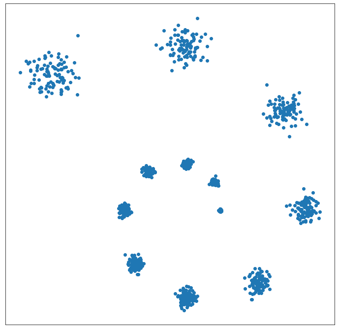
(a) Synthetic dataset.

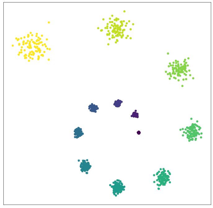
(b) Optimal clustering.

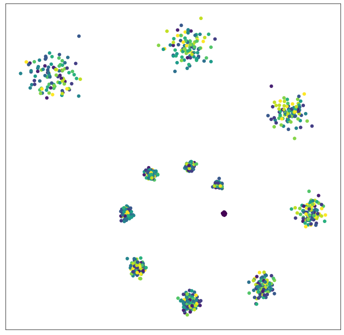
(c) Suboptimal clustering.

Figure 2: (a) A synthetic dataset, (b) its optimal clustering solution, (c) suboptimal clustering solution. The micro-averaged silhouette score $S_{micro}$ of the optimal solution is 0.74, which drops to -0.20 when the points in all clusters, except for the compact (low-variance) cluster, in the center are randomly assigned a cluster label.

When clusters are perfectly balanced, the sample mean (i.e., micro-averaging) is a reasonable aggregation strategy. This assumption, however, of clusters being perfectly balanced, cannot be guaranteed in the real world, where clusters are often imbalanced (see, for example, Table 1). In this case, micro-averaging is not effective, as will be discussed next in more detail. By contrast, the cluster-level (macro) aggregation strategy is more robust. In this strategy, a silhouette score $S_{c}$ is computed for each cluster $C_{i}$ as follows:

$$S_{C}(C_{i})=\frac{1}{|C_{i}|}\sum_{x_{i}\in C_{i}}s(x_{i}).$$ (5)

Hence, for each cluster $C_{i}$ a single silhouette value $S_{c_{i}}$ is computed, known as cluster mean silhouette. This value can be interpreted as a score that measures how compact and well separated a cluster given a clustering solution. Consequently, we end up with a set of $K$ silhouette values {$S_{C_{1}},\ldots,S_{C_{K}}$}, where $K$ is the number of clusters in the solution. To evaluate the clustering solution as a whole, the mean aggregates these $K$ scores into a single value. Although the mean is a straightforward option, we note that other statistics can also be used for this aggregation (e.g., min, max, median). More formally, this macro-averaged silhouette variant (i.e., equally weighing the clusters) is defined as follows:

$$S_{macro}(X)=\frac{1}{K}\sum_{k=1}^{K}S_{C}(C_{i}).$$ (6)

3.3 An imbalanced clustering example

Consider the synthetic dataset shown in Figure 2(a), which consists of $12$ Gaussian clusters with $100$ data points each. The clusters are of different variance, ranging from low to high values. Figure 2(b) presents the perfect clustering, where points in the same cluster are coloured similarly. The micro-averaged silhouette score $S_{micro}$ of this perfect clustering is $0.74$. Figure 2(c) shows the same data points as in Figure 2(b), but a random cluster assignment is hypothesised for all data points, except for those belonging to the compact low-variance cluster (nucleus) lying at the center of the dataset. For this suboptimal clustering, $S_{micro}$ drops to $-0.20$. Then, we disturb the cluster balance by adding points to the nucleus cluster, using a very small variance to preserve its dense structure, and we evaluated how the increase in cluster imbalance affects the $S_{micro}$ score. Figure 3 shows that the score increases monotonically with the nucleus size and it even exceeds the score of the correct partition for size above $5,000$ data points. $S_{macro}$, on the other hand, has a value of $-0.20$ at all cases of this random cluster assignment and a value of 0.74 for the perfect clustering.

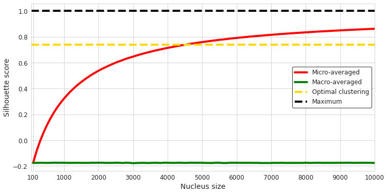
Figure 3: Micro- and macro-averaged silhouette (vertically) as a function of the size of the nucleus cluster (Figure 2(c)). The score for the optimal clustering (Figure 2(b)) is shown in yellow. In black is shown the highest possible silhouette score.

3.4 Cluster-balanced sampling for silhouette computation

The computation of the silhouette coefficient for all the $N$ points in a dataset requires the computation of a pairwise distance matrix at the cost of $\mathcal{O}(N^{2})$ operations. This is demanding in terms of computational and space complexity and, hence, not scalable for large datasets [19]. The typical approach to tackle this problem is to compute the silhouette score using a uniformly selected subsample of the dataset. In a cluster-imbalanced problem, the typical (uniform across data points) sampling may favour the major cluster and may even disregard completely one of the minor clusters. For example, considering the dataset of Figure 2 that contains the very dense nucleus cluster, the silhouette score was often impossible to compute when using the typical sampling strategy, since only data points from the nucleus cluster were sampled.

To solve this problem, following the intuition of the macro-averaged silhouette score, we propose creating a subsample of size $L$ for computing the macro-averaged silhouette score by uniformly selecting a subset of $L/K$ points from each cluster $C_{i}$, where $i=1,\ldots,K$. In this way, we ensure that all the clusters contribute a sufficient number of data points to the subsample, and a robust macro-averaged silhouette score computation.

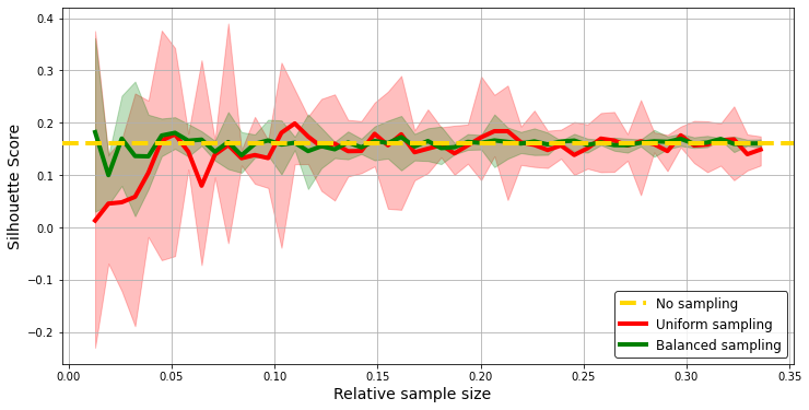
Figure 4: Macro-averaged silhouette values (vertically) as a function of the size of the typical uniform across data points (red) and the proposed balanced per-cluster (green) sample. The median (solid line) and the inter-whisker range (shadowed) from $30$ Monte Carlo simulations are shown.

Figure 4 presents a comparison between the typical (i.e., uniformly across data points) and the proposed cluster-balanced sampling of the macro-averaged silhouette score. The median for both strategies converges to the value achieved when using the whole dataset (yellow, dashed line), as expected. However, when using the typical uniform sampling strategy (red line), the macro-averaged silhouette score considerably varies (red shadow), especially for small sample sizes. By contrast, the variation is small when using the balanced strategy (green shadow), converging faster to a small value as the sample size increases.

3.5 Estimating the true number of clusters

One of the typical uses of silhouette is to estimate the number of clusters. This is achieved by solving the clustering problem for several $K$ values and selecting the solution with the maximum silhouette score [20].

To study the effect of imbalance on estimating the number of clusters we consider again the synthetic dataset of Figure 2. Each cluster consists of $100$ data points, except for the compact nucleus cluster that contains $10,000$ points. Using this dataset and for number of clusters $k\in[2,30]$, we have applied the global $k$-means++ [21], which is a fast variant of the global $k$-means method [22] employing the $k$-means++ [23] seed selection.

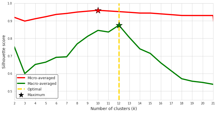
Figure 5: Estimating of number of clusters $k$ using the micro-averaged and macro-averaged silhouette using a synthetic dataset with imbalanced clusters.

Figure 5 shows the silhouette score of the solutions for varying $k$, when it is macro- (green line) and micro-averaged (red line). A star indicates the maximum per line. The macro-averaged score always finds the true number of clusters (yellow dashed vertical line), despite the heavy cluster imbalance. In contrast, the default micro-averaged scores are saturated near $0.95$ and a plateau for $k\in[6,15]$. The lack of a clear peak leads to the wrong estimation for the true number of clusters.

3.6 Sensitivity to background noise

Besides its sensitivity on cluster imbalance, shown in the previous paragraphs, we present another weakness of the micro-averaged silhouette score that is related to the existence of background noise, i.e., points lie between clusters or far from the clusters.

Figure 6(a) depicts four well-separated Gaussian clusters, each comprising $200$ data points. We introduced background random noise to this dataset, by sampling $n$ points from a uniform distribution $\epsilon_{n}\sim\mathcal{U}(a,b)$, with $a,b$ chosen so that the samples are spread uniformly in the data space, as shown in Figure 6(d). If $n$ noisy points are added, we define the relative level of background noise that is added to a dataset $X$ as $\frac{n}{n+|X|}\times 100\%$, As an example, Figure 6(b) (6(c)) presents the original dataset with 25% (50%) of background noise.

We generated several datasets (i.e., versions of the original dataset) by increasing the noise level. To each such dataset we applied global $k$-means++, with $k$ ranging from 1 to 30, and we computed the micro- and macro-averaged silhouette scores per $k$. The $k$ with the highest score was considered as the estimated correct number of clusters per dataset. Figure 6(d) presents the number of clusters estimation with respect to the noise level, where it can be seen that the macro-averaged score always provides the correct number of clusters. In contrast, the estimations using the micro score are severely affected as the noise level increases.

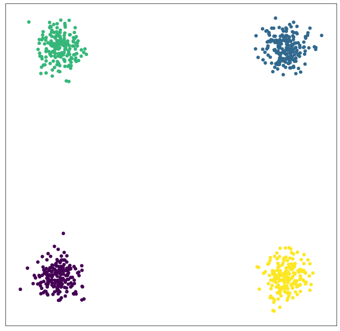
(a) Original dataset

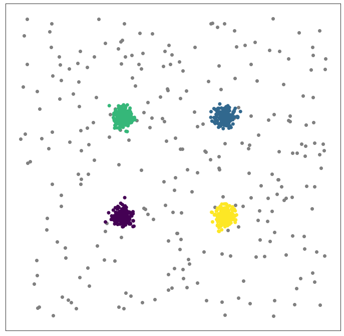
(b) $25\%$ is background noise

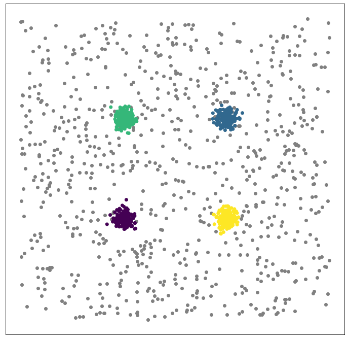
(c) $50\%$ is background noise

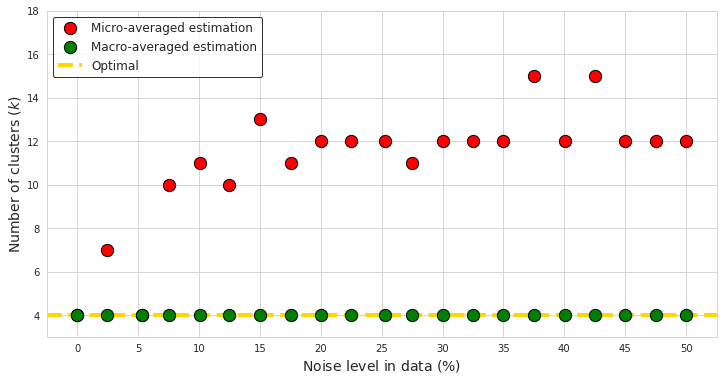
(d) Estimated number of clusters (vertically) per background noise level (horizontally) using micro- and macro-averaged silhouette scores

Figure 6: Synthetic dataset with four Gaussian clusters (a), focalised for visibility. Random background noise is added, consisting of 25% (b) and 50% (c) of the data while the estimated number of clusters is depicted per background noise level included in the data (d).

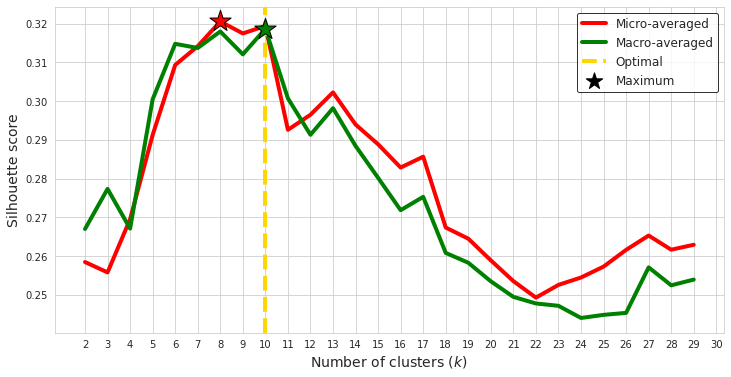
(a) pendigits

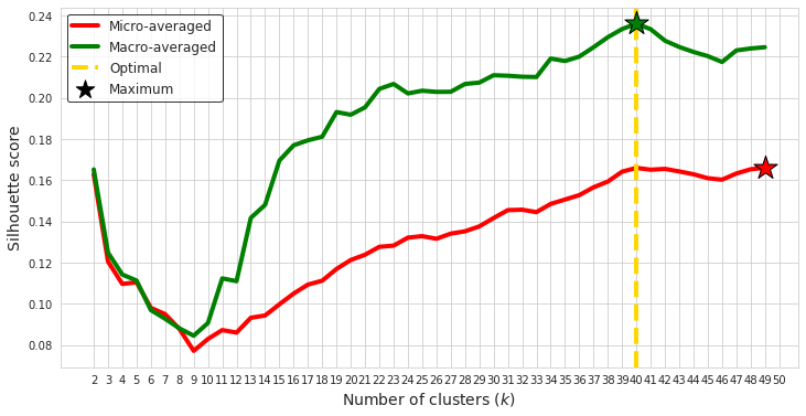
(b) olivetti faces

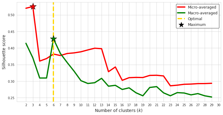
(c) glass

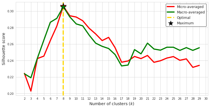
(d) mice

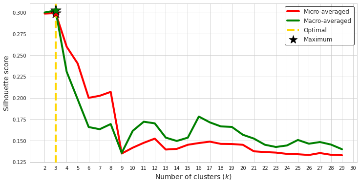
(e) wine

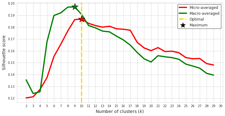
(f) optdigits

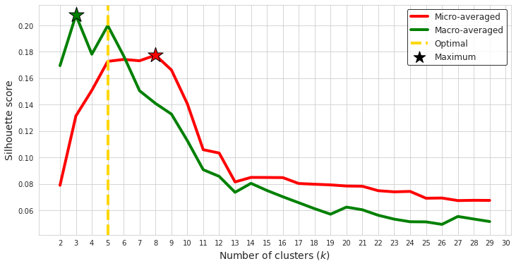
(g) tcga

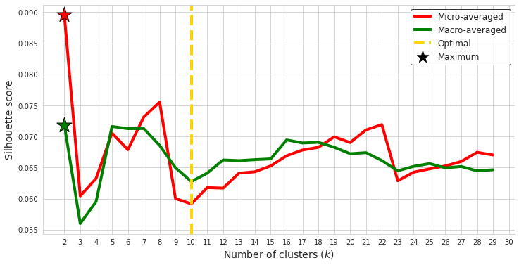
(h) mnist

Figure 7: Micro- (red) and macro-averaged (green) silhouette score per dataset, evaluating the partitions of $k$-means for varying $k$ values.

4 Experimental study

In the preceding section, we discussed the limitations associated with the micro-averaging strategy and underscored the robustness demonstrated by the macro-averaging strategy, in the context of controlled experiments with synthetic datasets. This section describes our experiments on real-world data, to provide an evaluation of the performance exhibited by both strategies in estimating the number of clusters.

4.1 Datasets

We have considered eight real-world datasets, summarised in Table 1 and characterised by a diverse number of data points (from one hundred to ten thousands), dimensionality (from nine to twenty thousand features), true number of clusters (from three to forty), and cluster imbalance (from $0.12$ to $1.00$).

Table 1: Real-world datasets ranked based on size ($N$), showing their number of input features ($d$), number of ground truth classes ($k$; considered as the ground truth number of clusters), and the ratio $r$ of the size of the minor to the major class.

Dataset	Type	Description	${N}$	${d}$	${k}$	$r$	Source
pendigits	Time-series	Handwritten digits	10,992	16	10	0.92	[24]
mnist (test)	Image	Handwritten digits	10,000	28$\times$28	10	0.79	[25]
optdigits	Image	Handwritten digits	5,620	8$\times$8	10	0.97	[24]
mice	Tabular	Expression levels of proteins	1,080	77	8	0.70	[24]
olivetti faces	Image	Human Faces	400	64$\times$64	40	1.00	at&t
tcga	Tabular	Cancer gene expression profiles	801	20,531	5	0.26	[24]
glass	Tabular	Types of glass	214	9	6	0.12	[24]
wine	Tabular	Chemical analysis of wines	178	13	3	0.68	[24]

The pendigits, mnist (test set), and optdigits datasets comprise handwritten digits, with $10$ classes corresponding to the digits from $0$ to $9$. optdigits consists of images with a resolution of $8\times 8$, while mnist contains images of a higher resolution (i.e., $28\times 28$). By contrast, pendigits’ data instances are represented by $16$-dimensional vectors containing pixel coordinates. The olivetti faces dataset contains facial images from $40$ different individuals with each person contributing a set of $10$ images of resolution $64\times 64$, capturing facial expressions, resulting to a dataset of $400$ samples in total.

The tcga dataset is a collection of gene expression profiles obtained from RNA sequencing of various cancer samples. It includes $801$ data instances, clinical information, normalised counts, gene annotations, and $6$ cancer types’ pathways. The Mice Protein Expression (mice) dataset consists of the expression levels of 77 proteins/protein modifications that produced detectable signals in the nuclear fraction of the cortex. It includes $1,080$ data points and $8$ eight classes of mice based on the genotype, behaviour, and treatment characteristics.

The glass and wine datasets encapsulate chemical analyses of glass types and wines, respectively. In the case of glass, it includes $9$ features that correspond to oxide content and provide characteristics features for $6$ different glass types. On the other hand, wine encompasses $13$ features derived from chemical analysis, representing different compositions, and is associated with $3$ distinct wine origins.

4.2 Experimental results

As with the synthetic dataset we have used the global $k$-means++ algorithm [21] to cluster each dataset for increasing values of $k$. Then, we measured the silhouette score for each solution ($k$), by employing both micro- and macro-averaging. The best clustering solution with respect to each score is selected for each dataset. All the datasets comprise ground truth ($k$ in Table 1), hence it is reasonable to expect that the maximum silhouette score would be observed at that number of clusters, disregarding the aggregation strategy.

Settings

We varied $k$ from $2$ to $30$. As a preprocessing step, we used min-max normalisation to map the attributes of each dataset to the $[0,1]$ interval to prevent attributes with large value ranges from dominating the distance calculations, and to also avoid numerical instabilities in the computations [26]. For the olivetti faces dataset, we varied $k$ up to $50$, due to its increased ground truth number of clusters. For the mice dataset, we applied one-hot encoding to manage categorical values and we imputed missing values by utilising the mean values for each column.

Correct number of clusters found

Figure 7 depicts the micro- and macro-averaged silhouette score per dataset. When we used the macro-averaging strategy (green line), the optimal score (starred) coincides with the ground truth (the yellow dashed line) in five out of eight datasets (pendigits, olivetti faces, glass, mice, wine), covering all the different data types (time-series, image, tabular data). When using micro-averaging (red line), the ground truth $k$ was correctly estimated in three datasets (mice, wine, optdigits). These three datasets cover two data types (image, tabular) and for the latter ones the ground truth was also correctly estimated when macro-averaging (overlapping stars).

Correct number of clusters not found

In one tabular dataset (tcga), both strategies failed to capture the ground truth. In two datasets (optdigits, tcga), the maximum macro-averaged silhouette was observed for a $k$ other than the ones defined in the ground truth. In optdigits, where the ground truth is defined as one cluster per digit ($k=10$), the best macro-average score is established when the digits 3 and 9 are clustered together. A similar observation can be drawn by looking at the red curve, where the best micro-averaged silhouette score is in a plateau covering two solutions, i.e., $k\in\{9,10\}$. A similar red plateau is observed for the tcga dataset, where the best solution could be any from a range, i.e., $5\leq k\leq 8$. On the contrary, macro-averaging suggests a solution ($k=3$) that falls out of that range. Interestingly, however, the second highest peak is at the true number of clusters (i.e., 5).

Silhouette ineffectiveness

There are also cases where the silhouette score is not effective with both aggregation strategies. Such a case can be observed in the mnist dataset where both aggregation strategies prefer the solution with $K=2$, while the ground-truth number of clusters is $K=10$. We note, however, that even the ground truth solution yields very low silhouettes scores ($S_{micro}\approx 0.049$, $S_{macro}\approx 0.045$). Although similar to optdigits in nature (i.e., images of nine handwritten digits), the complexity of the mnist data is higher (i.e., more dimensions and complicated digit patterns), yielding aggregated silhouette scores close to zero, thus both strategies fail in estimating the correct number of clusters.

5 Conclusions

In this work we revisited the widely-used silhouette coefficient, showing that the aggregation strategy should not be selected arbitrarily. Based on a synthetic example, we illustrated that the micro-averaged silhouette score for evaluating clustering solutions suffers from two key weaknesses due to its sensitivity to cluster imbalance and background noise. By contrast, as we show, the macro-averaged silhouette is robust to both these issues. Inspired by the macro-averaged strategy, we proposed a novel sampling strategy, which is considerably more robust compared to uniform sampling. By applying clustering on eight well-known real-world datasets, for various values of $K$, we assessed the two silhouette aggregation strategies regarding their ability to yield a maximum silhouette score for the ground truth number of clusters. Our experimental results show that the macro-averaged strategy leads to better estimations overall, but there is no clear winner, indicating that the use of both strategies when aggregating silhouette is the best option.

References

- [1] Peter J Rousseeuw. Silhouettes: a graphical aid to the interpretation and validation of cluster analysis. Journal of computational and applied mathematics, 20:53–65, 1987.
- [2] Robert Layton, Paul Watters, and Richard Dazeley. Evaluating authorship distance methods using the positive silhouette coefficient. Natural Language Engineering, 19(4):517–535, 2013.
- [3] Prafulla Bafna, Dhanya Pramod, and Anagha Vaidya. Document clustering: Tf-idf approach. In 2016 International Conference on Electrical, Electronics, and Optimization Techniques (ICEEOT), pages 61–66. IEEE, 2016.
- [4] Handrea Bernando Tambunan, Dhany Harmeidy Barus, Joko Hartono, Aji Suryo Alam, Dimas Aji Nugraha, and Hakim Habibi Hidayatullah Usman. Electrical peak load clustering analysis using k-means algorithm and silhouette coefficient. In 2020 International Conference on Technology and Policy in Energy and Electric Power (ICT-PEP), pages 258–262. IEEE, 2020.
- [5] Anil K Jain. Data clustering: 50 years beyond k-means. Pattern recognition letters, 31(8):651–666, 2010.
- [6] Absalom E Ezugwu, Abiodun M Ikotun, Olaide O Oyelade, Laith Abualigah, Jeffery O Agushaka, Christopher I Eke, and Andronicus A Akinyelu. A comprehensive survey of clustering algorithms: State-of-the-art machine learning applications, taxonomy, challenges, and future research prospects. Engineering Applications of Artificial Intelligence, 110:104743, 2022.
- [7] Anil K Jain, M Narasimha Murty, and Patrick J Flynn. Data clustering: a review. ACM computing surveys (CSUR), 31(3):264–323, 1999.
- [8] Ulrike Von Luxburg, Robert C Williamson, and Isabelle Guyon. Clustering: Science or art? In Proceedings of ICML workshop on unsupervised and transfer learning, pages 65–79. JMLR Workshop and Conference Proceedings, 2012.
- [9] Eréndira Rendón, Itzel Abundez, Alejandra Arizmendi, and Elvia M Quiroz. Internal versus external cluster validation indexes. International Journal of computers and communications, 5(1):27–34, 2011.
- [10] Pablo A Estévez, Michel Tesmer, Claudio A Perez, and Jacek M Zurada. Normalized mutual information feature selection. IEEE Transactions on neural networks, 20(2):189–201, 2009.
- [11] Nguyen Xuan Vinh, Julien Epps, and James Bailey. Information theoretic measures for clusterings comparison: Variants, properties, normalization and correction for chance. Journal of Machine Learning Research, 11(95):2837–2854, 2010.
- [12] Lawrence Hubert and Phipps Arabie. Comparing partitions. Journal of classification, 2(1):193–218, 1985.
- [13] José E Chacón and Ana I Rastrojo. Minimum adjusted rand index for two clusterings of a given size. Advances in Data Analysis and Classification, pages 1–9, 2022.
- [14] Tadeusz Caliński and Jerzy Harabasz. A dendrite method for cluster analysis. Communications in Statistics-theory and Methods, 3(1):1–27, 1974.
- [15] David L Davies and Donald W Bouldin. A cluster separation measure. IEEE transactions on pattern analysis and machine intelligence, (2):224–227, 1979.
- [16] Olatz Arbelaitz, Ibai Gurrutxaga, Javier Muguerza, Jesús M Pérez, and Iñigo Perona. An extensive comparative study of cluster validity indices. Pattern recognition, 46(1):243–256, 2013.
- [17] Fatima Batool and Christian Hennig. Clustering with the average silhouette width. Computational Statistics & Data Analysis, 158:107190, 2021.
- [18] Marcel Brun, Chao Sima, Jianping Hua, James Lowey, Brent Carroll, Edward Suh, and Edward R Dougherty. Model-based evaluation of clustering validation measures. Pattern recognition, 40(3):807–824, 2007.
- [19] Marco Capó, Aritz Pérez, and Jose A Lozano. Fast computation of cluster validity measures for bregman divergences and benefits. Pattern Recognition Letters, 170:100–105, 2023.
- [20] Erich Schubert. Stop using the elbow criterion for k-means and how to choose the number of clusters instead. ACM SIGKDD Explorations Newsletter, 25(1):36–42, 2023.
- [21] Georgios Vardakas and Aristidis Likas. Global -means: an effective relaxation of the global -means clustering algorithm. arXiv preprint arXiv:2211.12271, 2022.
- [22] Aristidis Likas, Nikos Vlassis, and Jakob J Verbeek. The global k-means clustering algorithm. Pattern recognition, 36(2):451–461, 2003.
- [23] David Arthur and Sergei Vassilvitskii. K-means++ the advantages of careful seeding. In Proceedings of the eighteenth annual ACM-SIAM symposium on Discrete algorithms, pages 1027–1035, 2007.
- [24] Dheeru Dua and Casey Graff. Uci machine learning repository, 2017.
- [25] Yann LeCun and Corinna Cortes. MNIST handwritten digit database. 2010.
- [26] M Emre Celebi, Hassan A Kingravi, and Patricio A Vela. A comparative study of efficient initialization methods for the k-means clustering algorithm. Expert systems with applications, 40(1):200–210, 2013.