Ions and dipoles in electric field: Nonlinear polarization and field-dependent chemical reaction

Abstract

We investigate electric-field effects in dilute electrolytes with nonlinear polarization. As a first example of such systems, we add a dipolar component with a relatively large dipole moment $\mu_{0}$ to an aqueous electrolyte. As a second example, the solvent itself exhibits nonlinear polarization near charged objects. For such systems, we present a Ginzburg-Landau free energy and introduce field-dependent chemical potentials, entropy density, and stress tensor, which satisfy general thermodynamic relations. In the first example, the dipoles accumulate in high-field regions, as predicted by Abrashikin et al.$[$Phys.Rev.Lett. 99, 077801 (2007)$]$. Finally, we consider the case, where Bjerrum ion pairs form a dipolar component with nonlinear polarization. The Bjerrum dipoles accumulate in high-field regions, while field-induced dissociation was predicted by Onsager $[$J. Chem. Phys.2, 599 (1934)$]$. We present an expression for the field-dependent association constant $K(E)$, which depends on the field strength nonmonotonically.

I Introduction

The electrostatic interactions among electric charges and dipoles in a solvent are of central importance in various situations in soft matter physics Russel ; Stokes ; Is . In this paper, we consider dilute electrolytes composed of a waterlike liquid solvent, cations, anions, and a dipolar component with a dipole moment $\mu_{0}$. Andelman, Orland, and their coworkers (AO) An1 ; An2 ; An3 ; An4 proposed a dipolar Poisson-Boltzmann (dPB) equation, where the dipoles can respond to electric field nonlinearly and their polarization density ${\mbox{\boldmath$p$}}_{d}$ yields the effective charge density $-4\pi\nabla\cdot{\mbox{\boldmath$p$}}_{d}$. In their papers the dipolar component is the solvent itself. Theoretically, it can be different from the solvent with some changes of the equations. The dPB equation is a generalization of the classical Poisson-Boltzmann equation and is convenient to investigate the nonlinear polarization around charged objects. In particular, AO group concluded that the dipole density is increased by the factor $\sinh h/h$ with $h=\mu_{0}E/k_{B}T$ An1 , where $E=|{\mbox{\boldmath$E$}}|$ is the field strength, $T$ is the temperature, and $k_{B}$ is the Boltzmann constant. In this paper we show the following. The dipole accumulation in high-field regions occurs if the dipolar component is a dilute solute in a solvent. On the other hand, a nearly incompressible polar solvent is hardly enriched in high-field regions.

The physics of ion-dipole systems is even more intriguing if associated ion pairs, Bjerrum dipoles Bje ; Ma ; Fuoss ; Roij ; Dill ; Vegt , are treated to form a dipolar component. In electrolytes, association of free ions and dissociation of bounded ion pairs balance on the average in equilibrium, while strong acids in full dissociation have long been studied since the seminal work by Debye-Hückel Russel ; Is ; Debye ; McQ ; Stokes . Although not well known, OnsagerOnsager34 predicted that applied electric field enhances breakage of the ion bonding to increase dissociation. He intended to explain conductance increases in weak electrolytes under electric field (the Wien effect) Wien ; Eck ; Kaiser ; Korea . In his theory, the effect is significant for $E\gtrsim 2k_{B}T/e\ell_{B}(=0.08$V$/$nm for ambient water), where $e$ is the elementary charge and $\ell_{B}$ is the Bjerrum length. Therefore, in high-field regions, some fraction of the Bjerrum dipoles dissociate in the Onsager theory, while dipoles of a dilute dipolar component accumulate without chemical reactions in the AO theory.

In treating the Coulombic and dipolar interactions, AO group used a Hubbard-Stratonovich transformation of the grand-canonical partition function. In this paper, we propose a Ginzburg-Landau free energy of electrolytes, where the polarization can be nonlinear in inhomogeneous electric field. With this approach we can draw unambiguous conclutions systematically. Because the problem is complex, we divide this paper into three parts: (i) A dipolar component is added as a dilute solute, (ii) the solvent exhibits nonlinear polarization in Sec.III, and (iii) Bjerrum ion pairs form a dipolar component in Sec.IV. There is no chemical reaction in the first two parts.

In our problem, we need to develop a thermodynamic theory of inhomogeneous electrolytes. In their book, Landau and Lifshits Landau-e examined thermodynamics of dielectric fluids in electric field, providing explanations of the electrostriction effect Hakim ; Stell and the Maxwell stress tensor. It shows that the stress tensor is not diagonal and the scalar pressure is not well-defined in electric field in such fluids. In this paper, we use the Maxwell stress tensor for electrolytes and introduce field-dependent chemical potentials $\mu_{i}$ and entropy density $S$. We find that these variables satisfy general thermodynamic relations. For Bjerrum dipoles, we determine the field-dependent association constant $K(E)$ using the field-dependent $\mu_{i}$. In the literature Bje ; Ma ; Fuoss ; Roij ; Dill ; Vegt ; Kirk ; Landau-s , the zero-field association constant $K(0)$ has been discussed. We can then examine the distributions of ions and dipoles near charged surfaces, incorporating the AO and Onsager theories.

The organization of this paper is as follows. In Sec.II, we will present a theromodynamics theory of dilute electrolytes consisting of four-components in electric field. In Sec.III, we will examine dilute electrolytes consisting of a polar solvent and a strong acid, where the solvent exhibits nonlinear polarization. In Sec.IV, we will investigate association and dissociation in electrolytes in electric field, where Bjerrum dipoles constitute the fourth component. In Appendix A, we will derive the electric free energy density using the Onsager theory of rodlike molecules Onsager49 .

II Thermodynamics of dilute electrolytes in electric field

In this section, we treat a four component system composed of a single-component polar solvent (1), cations with charge $Ze$ (2), anions with charge $-Ze$ (3), and a dipolar component with a molecular dipole moment $\mu_{0}$ (4). Here, $Z=1$ for monovalent salts (NaCl) and $Z=2$ for divalent salts (MgSO₄). We assume that the solvent dipole moment is considerably smaller than $\mu_{0}$ and the ions have no dipole moment, so the solvent exhibits linear polarization. As a typical solvent, we can suppose ambient liquid water at $T=300$ K and $p=1$ atm. In this paper, we use the cgs units.

II.1 Polarization of dipolar component

In our continuum theory, the densities $n_{i}({\mbox{\boldmath$r$}})$ of the four components are coarse-grained ones with spatial scales longer than the Bjerrum length $\ell_{B}=e^{2}/\epsilon_{\rm w}k_{B}T$, where $\epsilon_{\rm w}$ is the pure-solvent dielectric constant. The electric potential $\Phi$ and the electric field ${\mbox{\boldmath$E$}}=-\nabla\Phi$ also vary smoothly. To apply electric field, we suppose parallel charged plates separated by a distance $L$, within which an electrolyte is inserted in the region $0<z<L$. The lateral dimensions of the container much exceed $L$ and the edge effect is negligible.

The charge density $\rho$ and the polarization ${\mbox{\boldmath$p$}}_{d}$ of the dipolar component are written as

$$\rho=Ze(n_{2}-n_{3}),~{}~{}~{}{\mbox{\boldmath$p$}}_{d}=n_{4}{\mbox{\boldmath$\mu$}}_{d},$$ (1)

where ${\mbox{\boldmath$\mu$}}_{d}({\mbox{\boldmath$r$}})$ is the average dipole moment vector of the dipolar component per particle, as will be defined in Eq.(7) below. The polarization of the solvent molecules is expressed in the linear response form,

$${\mbox{\boldmath$p$}}_{\rm w}=(4\pi)^{-1}(\epsilon-1){\mbox{\boldmath$E$}}.$$ (2)

We then introduce the electric induction,

$${\mbox{\boldmath$D$}}={\mbox{\boldmath$E$}}+4\pi({\mbox{\boldmath$p$}}_{\rm w}+{\mbox{\boldmath$p$}}_{d})=\epsilon{\mbox{\boldmath$E$}}+4\pi{\mbox{\boldmath$p$}}_{d},$$ (3)

which is related to $\rho$ by the Poisson equation,

$$\nabla\cdot{\mbox{\boldmath$D$}}=\nabla\cdot(\epsilon{\mbox{\boldmath$E$}}+4\pi{\mbox{\boldmath$p$}}_{d})=4\pi\rho.$$ (4)

As shown in Eqs.(2) and (3), $\epsilon$ is the linear dielectric constant of the solvent molecules in the static limit. In dielectric experiments of 1:1 small salts in liquid water Co ; Wei ; Bu , $\epsilon$ decreased as $\Delta\epsilon=\epsilon-\epsilon_{{\rm w}}\cong-A_{1}c$ for the salt concentration $c$ below 1M$/\ell$, where $A_{1}$ is a constant. Here, $\Delta\epsilon$ ranged from $-8$ to $-20$ at $c\sim 1$M$/\ell$ depending on the salt species. This large decrease arises from the formation of the hydration shells of water around ions. That is, the water molecules inside the shells do not freely rotate due to the ion-dipole interaction and their contribution to $\epsilon$ is largely suppressed. For small $n_{i}$ ($i\geq 2$) we thus express $\epsilon$ as

$$\epsilon=\epsilon_{{\rm w}}(n_{1},T)+{\sum}_{i}^{\prime}\epsilon_{i}^{{\rm w}}(n_{1},T)n_{i}+\cdots,$$ (5)

where the coefficients $\epsilon_{i}^{{\rm w}}$ are independent of $n_{i}$ $(i\geq 2$). Hereafter, ${\sum}_{i}^{\prime}$ denotes summation over the solute species. Since $n_{2}=n_{3}$ on the average, the degree of hydration is indicated by the dimensionless coefficient,

$${\hat{\gamma}}=-n_{1}(\epsilon_{2}^{\rm w}+\epsilon_{3}^{\rm w})/2\epsilon_{\rm w},$$ (6)

which is positive in the range $2.5\lesssim{\hat{\gamma}}\lesssim 6$ (even divided by $2\epsilon_{\rm w}=160$). Thus, $\Delta\epsilon/\epsilon_{{\rm w}}\cong-\hat{\gamma}(n_{2}+n_{3})/n_{1}$ for 1:1 salts with $c\lesssim 1$M$/\ell$ in water. For larger $c$, Buchner et al. Bu obtained $\Delta\epsilon\cong-A_{1}c+A_{2}c^{3/2}$ with $A_{1}$ and $A_{2}$ being positive constants. For NaCl they argued that the degradation of $\epsilon$ is mostly due to Na cations. In Eq.(5) we add the term $\epsilon_{4}^{\rm w}n_{4}$ in case the dipolar particles affect the solvent polarization.

The dipole moment vector ${\mbox{\boldmath$\mu$}}_{d}$ in Eq.(1) is the statistical average defined by

$${\mbox{\boldmath$\mu$}}_{d}=\mu_{0}\langle{{\mbox{\boldmath$n$}}_{d}}\rangle=\frac{\mu_{0}}{4\pi}\int d\Omega P({\mbox{\boldmath$n$}}_{d},{\mbox{\boldmath$r$}}){\mbox{\boldmath$n$}}_{d},$$ (7)

where ${\mbox{\boldmath$n$}}_{d}$ is the microscopic unit vector along the dipole direction, $\int d\Omega$ is the angle integration of ${\mbox{\boldmath$n$}}_{d}$, and $P({\mbox{\boldmath$n$}}_{d},{\mbox{\boldmath$r$}})$ is the angle distribution function at position $r$ with $\int d\Omega P({\mbox{\boldmath$n$}}_{d},{\mbox{\boldmath$r$}})=4\pi$. In Appendix A, we shall see that the equilibrium form of $P({\mbox{\boldmath$n$}}_{d},{\mbox{\boldmath$r$}})$ in the dilute reime is written in terms of the local electric field ${\mbox{\boldmath$E$}}({\mbox{\boldmath$r$}})$ as

$$P({\mbox{\boldmath$n$}}_{d},{\mbox{\boldmath$r$}})={\cal N}_{\rm d}^{-1}\exp[\mu_{0}{\mbox{\boldmath$n$}}_{d}\cdot{\mbox{\boldmath$E$}}({\mbox{\boldmath$r$}})/k_{B}T],$$ (8)

Here, ${\cal N}_{\rm d}$ is the normalization factor,

$${\cal N}_{\rm d}=\frac{1}{4\pi}\int d{\Omega}\exp[\mu_{0}{\mbox{\boldmath$n$}}_{d}\cdot{\mbox{\boldmath$E$}}/k_{B}T]=\frac{\sinh h}{h}.$$ (9)

which depends on the dimensionless field strength,

$$h=\mu_{0}E/k_{B}T,$$ (10)

with $E=|{\mbox{\boldmath$E$}}|$. Here, we introduce $W(h)=\ln{\cal N}_{\rm d}$ and $W^{\prime}(h)=dW(h)/dh$ expressed as

$$W=\ln(\sinh h/h),~{}~{}~{}W^{\prime}={\cal L}(h)=\coth(h)-1/h,$$ (11)

where ${\cal L}(h)$ is the Langevin function with ${\cal L}\cong h/3$ for $h\ll 1$ and ${\cal L}\cong 1$ for $h\gg 1$. Then, Eqs.(7)-(9) give

$${\mbox{\boldmath$p$}}_{d}=n_{4}\mu_{0}{\cal L}(h)E^{-1}{{\mbox{\boldmath$E$}}}={\chi}_{d}{\mbox{\boldmath$E$}}.$$ (12)

Here, ${\chi}_{d}(h)=n_{4}\mu_{0}{\cal L}(h)/E$ is the nonlinear susceptibility of the dipolar component. Setting ${\mbox{\boldmath$D$}}=\epsilon_{\rm eff}{\mbox{\boldmath$E$}}$, we obtain the total nonlinear dielectric constant,

$$\epsilon_{\rm eff}=\epsilon+4\pi\chi_{d}=\epsilon+4\pi n_{4}\mu_{0}{\cal L}(h)/E.$$ (13)

As $h\to 0$ it follows the total linear dielectric constant,

$$\epsilon_{\rm eff}^{0}={\lim}_{h\to 0}\epsilon_{\rm eff}=\epsilon+4\pi(\mu_{0}^{2}/3k_{B}T)n_{4}.$$ (14)

For $h\gg 1$, the dipolar particles tend to fully align along $E$ with ${\chi}_{d}\cong n_{4}\mu_{0}/E$.

AO group An2 ; An4 calculated $\epsilon_{2}^{\rm w}$ and $\epsilon_{3}^{\rm w}$ using their dPB equation around ions, where the solvent (water) itself is the dipolar component. In our scheme, we assume their presence with large sizes from the beginning. Frydel Frydel constructed the dPB equation for ions with polarizabilities $\alpha_{i}$. The ionic polarization can be accounted for if we change $\epsilon_{i}^{\rm w}$ to $\epsilon_{i}^{\rm w}+4\pi\alpha_{i}$ in Eq.(5). However, $|\epsilon_{2}^{\rm w}+\epsilon_{3}^{\rm w}|$ is much larger than $4\pi\alpha_{i}$ for small ionsMadden .

II.2 Free energy functional and chemical potentials

We set up the free energy functional ${\cal F}=\int d{\mbox{\boldmath$r$}}f$, where the integration is within the cell confining the electrolyte solution. We neglect the van der Waals fluid-solid interaction and the image potential, which can be important near the surfaces, however. For $n_{i}\ll n_{1}$ ($i\geq 2$), the Helmholtz free energy density $f$ is written as Onukipolar ; anta ; Ben ; Oka1 ; Oka2

$$f=f_{\rm w}+k_{B}T{\sum}^{\prime}_{i}n_{i}[\ln(n_{i}\lambda_{i}^{3})+\nu_{i}-1]+f_{e},$$ (15)

where $f_{\rm w}(n_{1},T)$ is the pure-solvent free energy density without applied field. The first two terms constitute the non-electric part. For each $i(\geq 2)$, $\lambda_{i}(\propto T^{-1/2})$ is the thermal de Broglie length and $\nu_{i}(n_{1},T)$ consists of ideal-gas and interaction parts. The former is written as Landau-s ,

$$\nu_{i}^{0}(T)=-(k_{i}-3/2)\ln(T/\Theta_{i}^{0}),$$ (16)

where $2k_{i}-3$ is the degree of vibration-rotation freedom and $\Theta_{i}^{0}$ is a constant temperature. The difference $\Delta\nu_{i}=\nu_{i}-\nu_{i}^{0}$ is determined by the solute-solvent interactions at infinite dilution. Although not written in Eq.(15), the Debye-Hückel free energy density $f_{\rm DH}=-k_{B}T\kappa^{3}/12\pi$ Debye and the short-range ion-ion interaction terms are important to explain experimental data for not very dilute electrolytes McQ ; Stokes ; Oka2 , where $\kappa=Z[4\pi(n_{2}+n_{3})\ell_{B}]^{1/2}$ is the Debye wave number.

As will be shown in Appendix A, we use Onsager’s theory of rodlike molecules Onsager49 to obtain the electric free energy density $f_{e}$. Neglecting the short-range dipole-dipole interactions, we obtain

$$f_{e}=\epsilon E^{2}/8\pi+{\mbox{\boldmath$p$}}_{d}\cdot{\mbox{\boldmath$E$}}-k_{B}Tn_{4}W$$

$$=\epsilon E^{2}/8\pi+k_{B}Tn_{4}(hW^{\prime}-W).$$ (17)

where $W(h)$ and $W^{\prime}(h)$ are defined in Eq.(11). For $h\ll 1$, we have $W\cong h^{2}/6$ and $hW^{\prime}\cong h^{2}/3$, so $f_{e}$ tends to the linear response form,

$$f_{e}^{0}=\epsilon_{\rm eff}^{0}E^{2}/8\pi=(\epsilon+4\pi n_{4}\mu_{0}^{2}/3k_{B}T)E^{2}/8\pi.$$ (18)

Next, we slightly change $n_{i}$ and $T$ by $\delta n_{i}$ and $\delta T$. Then, from $\delta(\epsilon E^{2})=2{\mbox{\boldmath$E$}}\cdot\delta{\mbox{\boldmath$D$}}-8\pi{\mbox{\boldmath$E$}}\cdot\delta{\mbox{\boldmath$p$}}_{d}-E^{2}\delta\epsilon$ and ${\mbox{\boldmath$p$}}_{d}\cdot\delta{\mbox{\boldmath$E$}}=n_{4}\mu_{0}W^{\prime}\delta E$, $f_{e}$ is changed by

$$\delta f_{e}={\mbox{\boldmath$E$}}\cdot\delta{\mbox{\boldmath$D$}}/4\pi-E^{2}\delta\epsilon/8\pi$$

$$-(k_{B}TW)\delta n_{4}+k_{B}n_{4}(hW^{\prime}-W)\delta T.$$ (19)

Here, integration of the first term within the cell becomes

$$\frac{1}{4\pi}\int d{\mbox{\boldmath$r$}}{\mbox{\boldmath$E$}}\cdot\delta{\mbox{\boldmath$D$}}=\int d{\mbox{\boldmath$r$}}\Phi\delta\rho-(\Phi_{0}\delta Q_{0}+\Phi_{L}\delta Q_{L}),$$ (20)

where $(\Phi_{0},Q_{0})$ and $(\Phi_{L},Q_{L})$ are the surface potential and the surface charge at $z=0$ and $z=L$, respectively. If we assume the overall charge neutrality, we require

$$\int d{\mbox{\boldmath$r$}}\rho=Q_{0}+Q_{L},$$ (21)

under which we can replace $\Phi$ by $\Phi-C_{0}$ with $C_{0}$ being an arbitrary constant. The surface term in Eq.(20) vanishes at fixed surface charges $(\delta Q_{0}=\delta Q_{L}=0$).

We define the chemical potentials $\mu_{i}$ by the functional derivatives $\mu_{i}=\delta{\cal F}/\delta n_{i}$ at fixed $T$ and $n_{j}$ with $j\neq i$. Then, Eqs.(15), (19), and (20) give

$$\mu_{1}/k_{B}T=\mu_{\rm w}/k_{B}T+{\sum}^{\prime}_{i}\nu^{\prime}_{i}n_{i}-\zeta_{1},$$ (22)

$${\mu}_{2}/k_{B}T=\ln(n_{2}\lambda_{2}^{3})+\nu_{2}+U-\zeta_{2},$$ (23)

$${\mu}_{3}/k_{B}T=\ln(n_{3}\lambda_{3}^{3})+\nu_{3}-U-\zeta_{3},$$ (24)

$$\mu_{4}/k_{B}T=\ln(n_{4}\lambda_{4}^{3})+\nu_{4}-W-\zeta_{4},$$ (25)

where $\mu_{\rm w}(n_{1},T)=\partial f_{\rm w}/\partial n_{1}$ is the chemical potential of pure solvent. For each $i\geq 1$ we define

$$\zeta_{i}=\epsilon_{i}^{\prime}E^{2}/8\pi k_{B}T,$$ (26)

$$U=Ze\Phi/k_{B}T.$$ (27)

We write the density derivatives of $\nu_{i}$ and $\epsilon$ at fixed $T$ as

$$\nu^{\prime}_{i}=\partial\nu_{i}/\partial n_{1}~{}(i\geq 2),$$ (28)

$$\epsilon_{i}^{\prime}=\partial\epsilon/\partial n_{i}~{}(i\geq 1),$$ (29)

so $\epsilon_{1}^{\prime}\cong\partial\epsilon_{\rm w}/\partial n_{1}$ and $\epsilon_{i}^{\prime}\cong\epsilon_{i}^{\rm w}$ for dilute solutes. In Eq.(22), the last term $-\zeta_{1}$ gives rise to the electrostriction (see Eq.(50)) Landau-e ; Stell ; Hakim ; Kirk . In Eq.(23) and (24), the terms $-\zeta_{i}$ serve to increase $\mu_{i}$ in $E$ for $\epsilon_{i}^{{\rm w}}<0$ (see below Eq.(5)). In Eqs.(23)-(25), $\nu_{i}$ can be treated to be homogeneous constants in one-phase states. However, from their strong dependence on $n_{i}$, they exhibit discontinuities across interfaces in two-phase states, giving rise to solute density differences in the two phases.

We also define the entropy density as the functional derivative $S=-\delta{\cal F}/\delta T$ at fixed densities $\{n\}$ and fixed surface charges. The integral of ${\mbox{\boldmath$E$}}\cdot\delta{\mbox{\boldmath$D$}}/4\pi$ does not contribute to $S$ from Eq.(20) so that

$$S=S_{\rm w}-k_{B}{\sum}^{\prime}_{i}n_{i}\big{[}\ln(n_{i}\lambda_{i}^{3})-\frac{5}{2}+\nabla_{T}(T\nu_{i})\big{]}$$

$$+\frac{1}{8\pi}E^{2}\nabla_{T}{\epsilon}-k_{B}n_{4}(hW^{\prime}-W),$$ (30)

where $S_{\rm w}(n_{1},T)=-\partial f_{\rm w}/\partial T$ is the pure-solvent part and the last term is the entropy density of dipole orientation (see Appendix A). Here, $\nabla_{T}(\cdots)=\partial(\cdots)/\partial T$ denotes the temperature derivative at fixed densities $\{n\}$.

II.3 Free energy variations

As in Eq.(19) we consider small changes in $n_{i}$ and $T$. Then, the free energy density $f$ in Eq.(15) is changed by

$$\delta f={\sum}_{i}\mu_{i}\delta n_{i}-S\delta T-\nabla\cdot(\Phi\delta{\mbox{\boldmath$D$}})/4\pi,$$ (31)

where we use the field-dependent $\mu_{i}$ in Eqs.(22)-(25) and $S$ in Eq.(30). If the cell volume $V$ is fixed, the free energy increment $\delta{\cal F}=\int d{\mbox{\boldmath$r$}}\delta f$ is expressed as

$$\delta{\cal F}=\int d{\mbox{\boldmath$r$}}\Big{[}{\sum}_{i}\mu_{i}\delta n_{i}-S\delta T\Big{]}-\Phi_{0}\delta Q_{0}-\Phi_{L}\delta Q_{L},$$ (32)

Thus, ${\cal F}$ is used at fixed surface charges $\delta Q_{0}=\delta Q_{L}=0$.

If the potential difference $\Delta\Phi=\Phi_{0}-\Phi_{L}$ is fixed, we perform the Legendre transformation Landau-e ,

$$\tilde{\cal F}={\cal F}+\Phi_{0}Q_{0}+\Phi_{L}Q_{L}={\cal F}+\int d{\mbox{\boldmath$r$}}\big{[}\Phi\rho-\frac{1}{4\pi}{\mbox{\boldmath$E$}}\cdot{\mbox{\boldmath$D$}}\big{]}.$$ (33)

Setting $\tilde{\cal F}=\int d{\mbox{\boldmath$r$}}{\tilde{f}}$, we can define the electric free energy density ${\tilde{f}}_{e}$ by

$${\tilde{f}}_{e}=f_{e}+\Phi\rho-{{\mbox{\boldmath$E$}}\cdot{\mbox{\boldmath$D$}}}/{4\pi}$$

$$=\Phi\rho-{\epsilon E^{2}}/{8\pi}-k_{B}Tn_{4}W.$$ (34)

The incremental changes in $\tilde{f}$ and $\tilde{\cal F}$ are given by

$$\delta{\tilde{f}}={\sum}_{i}\mu_{i}\delta n_{i}-S\delta T+\nabla\cdot(\delta\Phi{\mbox{\boldmath$D$}})/4\pi,$$ (35)

$$\delta\tilde{\cal F}=\int d{\mbox{\boldmath$r$}}\Big{[}{\sum}_{i}\mu_{i}\delta n_{i}-S\delta T\Big{]}+Q_{0}\delta\Phi_{0}+Q_{L}\delta\Phi_{L}.$$ (36)

For $h\ll 1$, ${\tilde{f}}_{e}$ tends to $\Phi\rho-f_{e}^{0}$ with $f_{e}^{0}$ being given by Eq.(18), as it should be the case.

Previously, Ben-Yaakov et al. Ben used the electrostatic free energy density composed of the first two terms in the second line of Eq.(34), while we set it equal to $\epsilon E^{2}/8\pi$, the first term in Eq.(17) Onukipolar ; anta ; Oka2 . In these papers, the polarization was assumed to be linear.

II.4 Maxwell stress tensor

The solution stress tensor $\Pi_{\alpha\beta}$ consists of two parts,

$$\Pi_{\alpha\beta}=p_{\rm n}\delta_{\alpha\beta}+M_{\alpha\beta},$$ (37)

where $\alpha$ and $\beta$ stand for ($x,y,z)$ and

$$p_{\rm n}=p_{\rm w}+k_{B}T{\sum}^{\prime}_{i}(1+n_{1}\nu^{\prime}_{i})n_{i},$$ (38)

$$M_{\alpha\beta}=\frac{1}{8\pi}\big{(}\epsilon-{\sum}_{i}n_{i}\epsilon_{i}^{\prime}\big{)}E^{2}\delta_{\alpha\beta}-\frac{1}{4\pi}E_{\alpha}D_{\beta},$$ (39)

The $p_{\rm n}$ is the non-electric solution pressure arising from the first two terms in $f$ in Eq.(15) Oka2 with $p_{\rm w}(n_{1},T)=\partial f_{\rm w}/\partial n_{1}-f_{\rm w}$ being the pure-solvent pressure. The derivatives $\nu_{i}^{\prime}$ are related to the solute partial volumes (see Eq.(51)). The $M_{\alpha\beta}$ is the Maxwell stress tenor of the solution Landau-e with $D_{\beta}=\epsilon_{\rm eff}E_{\beta}$ and $M_{\alpha\beta}=M_{\beta\alpha}$, where $\epsilon_{i}^{\prime}$ are defined in Eq.(29). In its first term, $\epsilon-{\sum}_{i}n_{i}\epsilon_{i}^{\prime}$ is equal to $\epsilon_{\rm w}-n_{1}\epsilon_{1}^{\prime}$ to leading order in $n_{i}$ ($i\geq 2$) from $\epsilon$ in Eq.(5). It is also equal to $\epsilon_{\rm eff}^{0}-{\sum}_{i}n_{i}\partial\epsilon_{\rm eff}^{0}/\partial n_{i}$ in terms of $\epsilon_{\rm eff}^{0}$ in Eq.(14), so Eq.(39) surely tends to the linear polarization limit $\epsilon_{\rm eff}\to\epsilon_{\rm eff}^{0}$ in the Landau-Lifshits book. These authors presented $M_{\alpha\beta}$ for one-component dielectric fluids without ions in applied electric field (see Eq.(15.9) in their book Landau-e ). In this paper, we use it for dilute electrolytes containing dipoles with nonlinear polarization.

The reversible (non-dissipative) force density acting on the fluid is given by $-{\sum}_{\beta}\nabla_{\beta}\Pi_{\alpha\beta}$. From Eqs.(4), (12), and (39) its electric part is calculated as

$$-{\sum}_{\beta}\nabla_{\beta}M_{\alpha\beta}=\rho E_{\alpha}+{\mbox{\boldmath$p$}}_{d}\cdot\nabla E_{\alpha}$$

$$+{\sum}_{i}\nabla_{\alpha}(n_{i}\epsilon_{i}^{\prime}E^{2})/8\pi-{E^{2}}\nabla_{\alpha}\epsilon/8\pi,$$ (40)

where $\nabla_{\alpha}$ and $\nabla_{\beta}$ stand for the components of $\nabla=(\partial/\partial x,\partial/\partial y,\partial/\partial z)$. The second term can also be written as $\chi_{d}\nabla_{\alpha}E^{2}/2$ from $\nabla_{\beta}E_{\alpha}=\nabla_{\alpha}E_{\beta}$. In ${\sum}_{\beta}\nabla_{\beta}\Pi_{\alpha\beta}$, the pressure gradient $\nabla_{\alpha}p_{\rm n}$ is equal to the non-electric part of the combination ${\sum}_{i}n_{i}\nabla_{\alpha}\mu_{i}+S\nabla_{\alpha}T$ from the Gibbs-Duhem relation. We further confirm that ${\sum}_{\beta}\nabla_{\beta}M_{\alpha\beta}$ in Eq.(40) coincides with the electric part of this combination from Eqs.(22)-(25) and (30). Thus, we obtain

$${\sum}_{\beta}\nabla_{\beta}\Pi_{\alpha\beta}={\sum}_{i}n_{i}\nabla_{\alpha}\mu_{i}+S\nabla_{\alpha}T,$$ (41)

including the electric parts. The mechanical equililbrium ${\sum}_{\beta}\nabla_{\beta}\Pi_{\alpha\beta}=0$ is attained for homogeneous $\mu_{i}$ and $T$. We note that Eq.(41) can be used in the hydrodynamic equations of nonequilibrium electrolytes.

We can calculate the pressure contribution from the Debye-Hückel free energy $f_{\rm DH}=-k_{B}T\kappa^{3}/12\pi$ in the form $p_{\rm DH}=(1-3n_{1}\partial\ln\epsilon_{\rm w}/\partial n_{1})f_{\rm DH}/2$ Oka2 , where $\kappa$ is the Debye wave number. We can also derive this $p_{\rm DH}$ from the thermal average of $M_{ij}$ using the Debye-Hückel structure factor of the charge density McQ ; Stokes ; Debye . We note that $M_{ij}$ can be used in its nonlinear form for the thermal charge density fluctuations at small wave numbers in agreement with the Debye-Hückel theory.

II.5 Equilibrium solute densities

In equilibrium, the chemical potentials $\mu_{i}$ and the temperature $T$ are homogeneous constants. If we neglect the wall and image potentials, Eqs.(23)-(25) yield

$$n_{2}=n_{2}^{0}\exp(-\nu_{2}-U+\zeta_{2}),$$ (42)

$$n_{3}=n_{3}^{0}\exp(-\nu_{3}+U+\zeta_{3}),$$ (43)

$$n_{4}=n_{4}^{0}{\cal N}_{\rm d}\exp(-\nu_{4}+\zeta_{4}),$$ (44)

where $n_{i}^{0}$ ($i\geq 2)$ are constants independent of space, $\zeta_{i}$ are defined in Eq.(26). In Eqs.(42) and (43), $\zeta_{i}$ decrease $n_{i}$ for $\epsilon_{i}^{\rm w}<0$. Indeed, we find $\exp(\zeta_{i})=\exp(-0.05h^{2})$ ($i=2,3$) in ambient liquid water, where we set ${\hat{\gamma}}=3.5$ and $\epsilon_{2}^{\rm w}=\epsilon_{3}^{\rm w}$ in Eqs.(5) and (6) and $\mu_{0}=e\ell_{B}/2$ in Eq.(10). Despite this factor, $n_{3}$ ($n_{2})$ should increase near positively (negatively) charged surfaces, owing to the factor $e^{U}$ ($e^{-U}$). In Eq.(44), the factor ${\cal N}_{\rm d}(>1)$ in Eq.(9) comes from $-W$ in Eq.(25) amplifying $n_{4}$. AO group An1 found that the dipole density is multiplied by ${\cal N}_{d}$ (without $\nu_{i}$ and $\zeta_{i}$ in their expressions).

From Eqs.(12) and (44) the polarization ${\mbox{\boldmath$p$}}_{d}$ becomes

$${\mbox{\boldmath$p$}}_{d}=\mu_{0}n_{4}^{0}e^{-\nu_{4}+\zeta_{4}}{\cal G}(h)E^{-1}{\mbox{\boldmath$E$}},$$ (45)

where ${\cal G}(h)$ is defined by An1 ; An2 ; An4 ; An3

$${\cal G}(h)=\partial{\cal N}_{d}/\partial h={\cal N}_{d}{\cal L}(h)=\cosh h/h-\sinh h/h^{2}.$$ (46)

Now, Eq.(4) gives the four-component dPB equation,

$$\nabla\cdot\epsilon{\mbox{\boldmath$E$}}+4\pi\nabla\cdot{\mbox{\boldmath$p$}}_{d}=4\pi Ze(n_{2}-n_{3}),$$ (47)

where $n_{i}$ and ${\mbox{\boldmath$p$}}_{d}$ are given in Eqs.(42)-(45). We use the linear dielectric constant $\epsilon$ in Eq.(5), which depends on $n_{2}$ and $n_{3}$. The decrease of $\epsilon$ due to accumulation of cations or anions is crucial in solving Eq.(47) Roij1 , though not studied in this paper.

II.6 Density change of nearly incompressible solvent and osmotic stress

Next, we examine the equilibrium solvent density $n_{1}$ in a nearly incompressible solvent in a one-phase state. Its deviation is small if the solvent isothermal compressibility $\kappa_{T}^{\rm w}=(\partial n_{1}/\partial p)_{T}/n_{1}$ is much smaller than $1/k_{B}Tn_{1}$. For example, $k_{B}Tn_{1}\kappa_{T}^{\rm w}\cong 0.06$ in ambient liquid water. We can then expand $\mu_{\rm w}(n_{1},T)$ in Eq.(22) as

$$\delta\mu_{\rm w}=\mu_{\rm w}(n_{1},T)-\mu_{\rm w}(n_{1}^{0},T)=(n_{1}-n_{1}^{0})/n_{1}^{2}\kappa_{T}^{\rm w},\\$$ (48)

where $n_{1}^{0}$ is a constant reference density.

For simplicity, let the electrolyte be in equilibrium with a large pure solvent without applied field, for which $n_{1}^{0}$ is the solvent density in the reservoir. Here, the solvent chemical potential is common in the two regions as

$$\mu_{1}(\{n\},T)=\mu_{\rm w}(n_{1}^{0},T),$$ (49)

so Eq.(22) yields the solvent density deviation,

$$n_{1}/n_{1}^{0}-1=-n_{1}\kappa_{T}^{\rm w}k_{B}T[{\sum}_{i}^{\prime}\nu_{i}^{\prime}n_{i}-\zeta_{i}]$$

$$=-{\sum}_{i}^{\prime}v_{i}^{*}n_{i}+n_{1}\kappa_{T}^{\rm w}{\epsilon_{1}^{\prime}}E^{2}/8\pi.$$ (50)

For each $i\geq 2$, $v_{i}^{*}$ is a volume related to the partial volume ${\bar{v}}_{i}$ at infinite dilution Buff ; Oc ; Oka1 ; Oka2 as

$$v_{i}^{*}=n_{1}k_{B}T\kappa_{T}\nu_{i}^{\prime}={\bar{v}}_{i}-k_{B}T\kappa_{T}.$$ (51)

The difference ${\bar{v}}_{i}-v_{i}^{*}=k_{B}T\kappa_{T}^{\rm w}$ stems from the partial pressure $k_{B}Tn_{i}$ and is small, which is $0.06/n_{1}$ in ambient liquid water. In Eq.(50), the first term represents the steric effect Oka2 and the second term the electrostriction Landau-e ; Stell ; Hakim . Note that $v_{i}^{*}$ can be negative due to the hydration (see the last paragraph in this subsection). On the other hand, in the lattice theory of fluid mixtures, all the particles have a common volume $v_{0}$ and the space-filling relation ${\sum}_{i}v_{0}n_{i}=1$ is assumed PG ; Iglic ; An5 .

In the above situation we also calculate the equilibrium stress component $\Pi_{zz}$ in the one-dimensional geometry, where the electric field $E$ changes along the $z$ axis. Here, $p_{\rm w}(n_{1},T)=p_{0}+n_{1}\delta\mu_{\rm w}$, with $p_{0}$ being the reservoir pressure. From Eqs.(37)-(39), (48), and (50) we thus find Is

$$\Pi_{zz}=p_{0}+k_{B}T{\sum}_{i}^{\prime}n_{i}+(\epsilon_{\rm w}-2\epsilon_{\rm eff})E_{z}^{2}/8\pi.$$ (52)

From Eqs.(42)-(44) we confirm that the above $\Pi_{zz}$ is independent of $z$ (or $d\Pi_{zz}/dz=0$) in accord with Eq.(41).

We comment on the partial volumes of salts in ambient liquid water. In experiments with the overall charge neutrality, the sum ${\bar{v}}_{s}={\bar{v}}_{2}+{\bar{v}}_{3}$ has been measured. From data of ${\bar{v}}_{s}$ Mil ; Craig , $n_{1}({v}^{*}_{2}+{v}^{*}_{3})$ was $-0.20$, $-0.55$, $0.93$, and $2.0$ for LiF, MgSO₄, NaCl, and NaI, respectively. Then, $n_{1}(\nu_{2}^{\prime}+\nu_{3}^{\prime})$ is $-3.4$, $-10$, $15$, and $32$, respectively, for these salts. For small and/or multivalent ions, $v_{i}^{*}$ and $\nu_{i}^{\prime}$ are negative, while $\nu_{i}^{\prime}\gg 1$ for large ions.

III Solvent nonlinear polarization

In this section we consider equilibrium three-component electrolytes composed of a solvent, cations, and anions, where the solvent exhibits nonlinear polarization and is nearly incompressible. Indeed, AO group treated such electrolytes An1 ; An2 ; An3 ; An4 . In this case, the linear dielectric constant $\epsilon_{\rm w}$ of the solvent is given by

$$\epsilon_{\rm w}=1+4\pi\mu_{0}^{2}n_{1}/3k_{B}T.$$ (53)

Since the linear dielectric constant $\epsilon$ of the solution is given in Eq.(5), the nonlinear dielectric constant $\epsilon_{\rm eff}$ of the solution is expressed as

$$\epsilon_{\rm eff}=1+\epsilon-\epsilon_{\rm w}+n_{1}{\mu_{0}}E^{-1}{\cal L}(h).$$ (54)

where $\epsilon-\epsilon_{\rm w}\cong\epsilon_{2}^{\rm w}n_{2}+\epsilon_{3}^{\rm w}n_{3}$. See $\epsilon_{\rm eff}$ in Eq.(13) also. The electric free energy density is then given by

$$f_{e}=(1+\epsilon-\epsilon_{\rm w})E^{2}/8\pi+k_{B}Tn_{1}(hW^{\prime}-W),$$ (55)

which tends to $\epsilon E^{2}/8\pi$ as $h\to 0$ from Eq.(53). The increment $\delta f_{e}$ is obtained if we replace $\delta\epsilon$ by $\delta(\epsilon-\epsilon_{\rm w})$, $\delta n_{4}$ by $\delta n_{1}$, and $n_{4}$ by $n_{1}$ in Eq.(19). Then, it follows the solvent chemical potential,

$$\mu_{1}=\mu_{\rm w}(n_{1},T)+k_{B}T(\nu^{\prime}_{2}n_{2}+\nu^{\prime}_{3}n_{3})-k_{B}TW,$$ (56)

which should be compared with $\mu_{1}$ in Eq.(22). The expressions for $\mu_{2}$ and $\mu_{3}$ are still given by Eqs.(23) and (24). Notice that the last term $-k_{B}TW$ in Eq.(56) tends to the electrostriction term $-k_{B}T\zeta_{1}$ as $h\to 0$ from

$$k_{B}TW\cong k_{B}Th^{2}/6=(\partial\epsilon_{\rm w}/\partial n_{1})E^{2}/8\pi~{}~{}(h\ll 1).$$ (57)

We should consider the deviation of $n_{1}$. Let us determine the reference solvent density $n_{1}^{0}$ from the osmotic condition (49). As in Eq.(50), we find

$$n_{1}/n_{1}^{0}-1=-v_{2}^{*}n_{2}-v_{3}^{*}n_{3}+(k_{B}Tn_{1}\kappa_{T}^{\rm w})W.$$ (58)

The last term is small from $k_{B}Tn_{1}\kappa_{T}^{\rm w}\ll 1$ and $W\cong h$ for $h\gg 1$ (see the first paragraph in Sec.IIE). That is, the polarization-induced increase in $n_{1}$ is negligible for small solvent compressibility, while that in $n_{4}$ can be significant as found in Sec.II. Thus, regarding $n_{1}$ as a constant, we now set up the three-component dPB equation as

$$\nabla\cdot\big{[}1+\epsilon-\epsilon_{\rm w}+n_{1}{\mu_{0}}{E}^{-1}{\cal L}(h)\big{]}{\mbox{\boldmath$E$}}=4\pi Ze(n_{2}-n_{3}),$$ (59)

where $n_{4}^{0}e^{-\nu_{4}+\zeta_{4}}$ is replaced by $n_{1}$ and ${\cal G}={\cal N}_{d}{\cal L}$ by ${\cal L}$ in Eq.(45). Here, we neglect the steric effect due to the first two terms in the right hand side of Eq.(58).

In their three-component dPB equation, AO group used ${\cal G}$ instead of $\cal L$, where the polarization contribution is larger than in Eq.(59) by ${\cal N}_{d}$. See Eq.(5) in Ref.An1 and Eq.(27) in Ref.An3 . They further accounted for the steric effect dividing the polarization contribution and the charge density by ${\cal D}=(1-\phi_{0}){\cal N}_{d}+\phi_{0}\cosh(U)$, where $\phi_{0}$ is the bulk ion volume fraction. See Eq.(9) in Ref.An1 and Eq.(13) in Ref.An4 . However, as indicated by Eq.(58), we should divide them by An5 ; Iglic

$${\cal D}_{0}=1-\phi_{0}+\phi_{0}\cosh(U),$$ (60)

where all the particles are assumed to have the same volume (see below Eq.(51)). The steric effect is crucial in high-potential regions with $\phi_{0}\cosh(U)\gtrsim 1$.

IV Ion association and dissociation

In this section, we examine the equilibrium electric-field effect for Bjerrum dipoles composed of monovalent ions Bje ; Fuoss ; Roij ; Ma ; Dill ; Vegt . For simplicity, we assume that they have a fixed dipole length $\ell_{d}$ with a constant dipole moment,

$$\mu_{0}=e\ell_{d},$$ (61)

though $\ell_{d}$ should thermally fluctuate due to rather weak bonding. In the original theories of ion pairing Ma ; Bje ; Fuoss , $\ell_{d}$ is of order $\ell_{B}$. We then use the Onsager theory of the orientation entropy in Appendix A. For relatively high salt concentrations ($\gtrsim 1$M$/\ell$), clustering of ions becomes conspicuous in simulations Vegt ; Ma ; Deg ; Hassan .

On symmetric multivalent ion pairs (A^+ZB^-Z), we make comments here and in the last paragraph of this section. The dipole moment of such ion pairs is of order $Z^{3}e\ell_{B}$ if there separation length is of order $Z^{2}\ell_{B}$. However, this picture is not justified because a number of water molecules are nonlinearly oriented between them. Nevertheless, the electric field effect should be enhanced for multivalent ion pairs. It is worth noting that the chemical reaction of MgSO₄ is the main origin of low-frequency sound attenuation in sea water Yeager1 ; Sim ; Eigen , where the dissociation time is of order $10^{-6}$sec and is very long.

IV.1 Chemical equilibrium

In chemical thermodynamics Landau-s ; Kirk , the condition of chemical equilibrium is given by $\mu_{2}+\mu_{3}=\mu_{4}$, where dissociation and association balance on the average. This condition is rewritten as

$$\mu_{2}+\mu_{3}-\mu_{4}=k_{B}T\ln[Kn_{2}n_{3}/n_{1}n_{4}]=0,$$ (62)

where $K$ is the equilibrium association constant in the dimensionless form. From Eqs.(23)-(25) we have

$$\ln K=\ln[n_{1}(\lambda_{2}\lambda_{3}/\lambda_{4})^{3}]+\nu_{r}-W-\epsilon_{r}^{\prime}E^{2}/(8\pi k_{B}T),$$ (63)

where $\nu_{r}$ and $\epsilon_{r}^{\prime}$ are defined by

$$\nu_{r}=\nu_{2}+\nu_{3}-\nu_{4},$$ (64)

$$\epsilon_{r}^{\prime}=\epsilon_{2}^{\prime}+\epsilon_{3}^{\prime}-\epsilon_{4}^{\prime}\cong\epsilon_{2}^{\rm w}+\epsilon_{3}^{\rm w}-\epsilon_{4}^{\rm w}.$$ (65)

In experiments, $K$ is determined in equilibrium by

$$K=n_{1}n_{4}/n_{2}n_{3}=c_{4}/c_{2}c_{3},$$ (66)

where $c_{i}=n_{i}/n_{1}$ $(i\geq 2$) are the solute concentrations. Typically, $K=10^{2}$ for $Z=1$ and $K=10^{4}$ for $Z=2$ without applied field Ma ; Rie .

In $f$ in Eq.(15), $\nu_{4}$ is the parameter for the Bjerrum dipoles. If there is no applied field, its non-ideal part $\nu_{4}-\nu_{4}^{0}$ is determined by the Coulombic attraction between an associating ion pair under the influence of the solvent. For small 1:1 ion pairs, the mutual potential is given by $-(k_{B}T\ell_{B})/r$ if the separation distance $r$ is shorter than $\ell_{B}$ Bje ; Fuoss ; Ma ; Dill ; Vegt ; Roij . Bjerrum Bje and Fuoss Fuoss estimated $K$ as

$$K_{\rm B}\sim a^{3}\int_{a}^{\ell_{B}/2}drr^{2}e^{\ell_{B}/r},~{}~{}K_{\rm F}\sim e^{\ell_{B}/a},$$ (67)

respectively. Here, $a$ is the closest center-to-center distance of an ion pair. In Bjerrum’s theory, the bounded pairs are those with $a<r<\ell_{B}/2$. If we use their estimations, the association contribution to $\nu_{4}-\nu_{4}^{0}$ is given by $-\ln K_{\rm B}$ or $-\ln K_{\rm F}$ in the absence of applied field from Eqs.(63) and (64).

IV.2 Field-dependent association constant

In applied electric field $E$, the ion bonding tends to be partially broken when the dipole direction ${\mbox{\boldmath$n$}}_{d}$ is parallel to $E$, while the bonding is stronger for ${\mbox{\boldmath$n$}}_{d}\cdot\mbox{\boldmath$E$}<0$. The Wien effect for weak electrolytes Wien ; Eck ; Kaiser ; Korea indicates that the dissociation constant $K_{d}$ should increase with increasing $E=|\mbox{\boldmath$E$}|$, where $K_{d}$ is the inverse of the association constant $K$. For 1:1 salts, Onsager Onsager49 calculated the $E$-dependence of $K_{d}$ in the form,

$$K_{d}(E)/K_{d}(0)=F_{\rm O}(b)=I_{1}(\sqrt{8b})/\sqrt{2b}.$$ (68)

where $I_{1}(x)=\pi^{-1}\int_{0}^{\pi}d\theta\cos\theta\exp({x\cos\theta})$ is the modified Bessel function of the first kind and $b$ is given by

$$b=\ell_{B}eE/2k_{B}T=(\ell_{B}/2\ell_{d})h,$$ (69)

with $\ell_{d}$ being defined in Eq.(61). Here, $F_{\rm O}(b)\cong 1+b$ for $b\ll 1$ and $F_{\rm O}(b)\cong\sqrt{2/\pi}(8b)^{-3/4}\exp(\sqrt{8b})$ for $b\gg 1$. The characteristic field at $b=1$ is $E=2k_{B}T/e\ell_{B}=0.08$V$/$nm. In particular, $b=h$ for $\ell_{d}=\ell_{B}/2$. Onsager derived Eq.(68) kinetically from the equations for Brownian motion in the combined Coulomb and external fields. However, $K_{d}(=1/K)$ is determined by Eq.(62) in equilibrium, so it can be calculated by a static theory.

To understand the Onsager formula (68), let us assume that ${\mbox{\boldmath$n$}}_{d}$ is parallel to $E$. Then, the sum of the Coulombic potential and the field potential is written as

$$\psi_{B}(r)=-k_{B}T\ell_{B}/r-eEr.$$ (70)

which assumes a maximum $\psi_{B}^{\rm max}$ at $r=\ell_{B}/\sqrt{2b}$ with

$$\psi_{B}^{\rm max}/k_{B}T=-\sqrt{8b}.$$ (71)

Thus, we find $\sqrt{8b}$ in Eq.(68). However, in the above argument (and in Osager’s calculation also), the thermal random rotations of the dipoles are neglected, which should be important particularly for weak applied field.

In this paper, we treat the field-induced dissociation as a consequence of the field-induced potential change, as argued in the above paragraph. That is, we assume that $\nu_{4}$ in the chemical potential $\mu_{4}$ is field-dependent as

$$\nu_{4}(E)=\nu_{4}(0)+\ln F_{\rm O}(b),$$ (72)

where we use Onsager’s $F_{O}$. Then, $\mu_{4}$ in Eq.(25) becomes

$$\mu_{4}(E)=\mu_{4}(0)-k_{B}T\ln({\cal N}_{d}/F_{\rm O})-\epsilon_{4}^{\prime}E^{2}/8\pi.$$ (73)

Thus, in the presence of electric field, $\mu_{4}/k_{B}T$ decreases by $W=\ln{\cal N}_{d}$ due to the dipole alignment but increases by $\ln F_{\rm O}$ due to the potential change. Here, $W\propto h^{2}$ and $\ln F_{O}\propto h$ for small $h$. In Fig.1(a), we plot $\ln({\cal N}_{d}/F_{\rm O})$ for $b=h$ using Onsager’s $F_{O}$, where $F_{\rm O}$ is larger (smaller) than ${\cal N}_{d}$ for $h\lesssim 7$ (for $h\gtrsim 7$).

For 1:1 salts, Eqs.(63)-(65) and (72) yield the field-dependent association constant $K(E)$ in the form,

$$K(E)/K(0)=\exp(A_{r}h^{2}){\cal N}_{d}/F_{\rm O}(b).$$ (74)

If we use $\hat{\gamma}$ in Eq.(6) and set $\epsilon_{4}^{\prime}=0$, $A_{r}$ is written as

$$A_{r}=-(\epsilon_{2}^{\rm w}+\epsilon_{3}^{\rm w})k_{B}T/8\pi\mu_{0}^{2}={\hat{\gamma}}/(4\pi\ell_{B}\ell_{d}^{2}n_{1}).$$ (75)

In Fig.1(a), $K(E)/K(0)$ is plotted for $b=h$ and $A_{r}=0.10$, where the factor $\exp(A_{r}h^{2})$ is important for $h\gtrsim 3$. Thus, $K(E)$ decreases due to Onsager’s dissociation mechanism for relatively small $h(\lesssim 3)$, but it increases due to the dipole accumulation and the ion-induced dielectric degradation for larger $h$.

IV.3 Electric double layer with Bjerrum dipoles

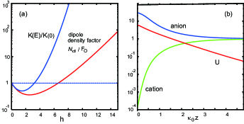
Figure 1: (a) Field-dependence of the association constant $K(E)/K(0)$ in Eq.(74) and the dipole density factor $c_{4}/c_{d}^{0}={\cal N}_{d}/F_{O}$ in Eq.(79) as functions of the normalized field strength $h=\mu_{0}E/k_{B}T$ in Eq.(10) for 1:1 salts on a semi-logarithmic scale. In $\mu_{4}$ in Eq.(73) $\ln({\cal N}_{d}/F_{O})$ also appears. (b) Near-wall profiles of $U(z)$ (electric potential), $c_{2}(z)/c_{0}$ (cation), and $c_{3}(z)/c_{0}$ (anion) vs $\kappa_{0}z$ on a semi-logarithmic scale, where the bulk concentrations are $c_{0}=c_{d}^{0}=10^{-2}$ and $\kappa_{0}$ is the bulk Debye wave number.

We consider an electric double layer with a charged surface at $z=0$ in the semi-infinite limit ($0<z<\infty$). For large $z$, $c_{2}(z)=n_{2}(z)/n_{1}$ and $c_{3}(z)=n_{3}(z)/n_{1}$ tend to $c_{0}$, while $c_{4}(z)=n_{4}(z)/n_{1}$ tends to $c_{d}^{0}$. From Eq.(66) the bulk concentrations $c_{0}$ and $c_{d}^{0}$ satisfy

$$c_{d}^{0}=K(0)c_{0}^{2}.$$ (76)

Neglecting the steric effect we write the solute concentration profiles $c_{i}(z)=n_{i}(z)/n_{1}$ as

$$c_{2}(z)=c_{0}\exp(-U-A_{2}h^{2}),$$ (77)

$$c_{3}(z)=c_{0}\exp(U-A_{3}h^{2}),$$ (78)

$$c_{4}(z)=c_{d}^{0}{\cal N}_{d}/F_{\rm O},$$ (79)

where $A_{i}=-\epsilon_{i}^{\rm w}k_{B}T/8\pi\mu_{0}^{2}$ ($i=2,3$) with $A_{2}+A_{3}=A_{r}$ for $\epsilon_{4}^{\prime}=0$. The $U(z)$ and $h(z)$ tend to 0 as $z\to\infty$. See Fig.1(a) for $c_{4}/c_{d}^{0}={\cal N}_{d}/F_{O}$ vs $h$.

In Fig.1(b), we plot $U(z)$ $c_{2}(z)/c_{0}$, and $c_{3}(z)/c_{0}$ vs $\kappa_{0}z$ for a 1:1 salt, where $c_{0}=c_{d}^{0}=10^{-2}$, $K(0)=10^{2}$, and $A_{2}=A_{3}=0.05$ with $\kappa_{0}$ being the bulk Debye wave number. In this example, $U$ exhibits a nearly exponential decay. The parameter values are common to those in (a).

Finally, we examine the dielectric constant $\epsilon_{\rm eff}$ in the bulk region for $Z:Z$ salts. From Eq.(14) it is written as

$$\epsilon_{\rm eff}/\epsilon_{\rm w}\cong 1-2{\hat{\gamma}}c_{0}+A_{d}c_{d}^{0},$$ (80)

where we use Eq.(6) with $\epsilon_{4}^{\rm w}=0$ in the second term. From Eqs.(14) and (57) the coefficient $A_{d}$ is given by

$$A_{d}=4\pi Z^{2}\ell_{B}\ell_{d}^{2}n_{1}/3.$$ (81)

For $Z=1$ and $\ell_{d}=\ell_{B}/2$, $A_{d}$ is about $12$. For multivalent ion pairs, $A_{d}$ is larger (see below Eq.(60)). Thus, the third dipolar term in Eq.(80) can exceed 1 for $c_{d}^{0}>A_{d}^{-1}$ or for $c_{0}>[A_{d}K(0)]^{-1/2}$, where the lower bound of $c_{0}$ is 0.03 for $Z=1$ and $1.5(\ell_{B}/2\ell_{d})\times 10^{-3}$ for $Z=2$. Here, we set $K(0)=10^{2}$ for $Z=1$ and $K(0)=10^{4}$ for $Z=2$ Ma ; Rie . If $c_{0}$ much exceeds the lower bound, we have $\epsilon_{\rm eff}\propto c_{0}^{2}$ and the Debye wave number becomes proportional to $[c_{0}/\epsilon_{\rm eff}]^{1/2}\propto c_{0}^{-1/2}$, as predicted by Zwanikken and Roij Roij . We also note that the second term in Eq.(80) serves to decrease $\epsilon_{\rm eff}$, which can also be important with increasing the $c_{0}$.

V Summary and remarks

We have studied the effects of electric field in dilute electrolytes, which contain dipoles exhibiting nonlinear polarization. Our main results are summarized below.

In Sec.II, we have discussed thermodynamics of electrolytes in inhomogeneous electric field, where the dipolar component is a dilute solute. The electric free energy density $f_{e}$ has been presented in Eq.(17) using Onsager’s theory Onsager49 . We have then defined the field-dependent chemical potentials $\mu_{i}$ in Eqs.(22)-(25) and the entropy density $S$ in Eq.(28). We have calculated the equilibrium density profiles of the solutes and the solvent in Eqs.(42)-(45) and (49). In Sec.III, we have considered three-component electrolytes (solvent+ strong acid), where the solvent polarization can be nonlinear. In this case, if the solvent is nearly incompressible, the solvent density increase due to nonlinear polarization is negligible, which is not in accord with the theory by the Andelman-Orland group. In Sec.IV, we have examined Bjerrum dipoles created by association and dissociation of 1:1 salts, which have a large dipole moment. We have calculated the density profiles in Eqs.(71)-(73) and the field-dependent association constant $K(E)$ in Eq.(68).

We make some remarks below. (i) The Debye-Hückel free energy density and the short-range ion-ion interaction terms are needed for not very dilute electrolytes McQ ; Stokes ; Oka2 . We should further include the steric effect in our theory to account for the accumulation of ions and dipoles near charged surfaces Iglic ; An5 ; Oka2 . We have also neglected the short-range solute-wall interactions and the image potentials. (ii) The decrement of the dielectric constant $\epsilon$ due to ions in Eq.(5) should greatly affect the ion densities near charged surfaces Roij1 , so its influence should be examined in detail. (iii) The Onsager theory of field-induced dissociation Onsager34 has not attracted enough attention, so his formula (68) should be checked in detail (see our remark below Eq.(71)). (iv) We should study the effect of electric field on electrolytes with multivalent salts such as MgSO₄ and MgCl₂. (v) Recently, the screening length has been shown to be longer than the Debye length $\kappa^{-1}$ in ionic liquids Is1 and concentrated electrolytes ($>1$M$/\ell$ for NaCl) Perkin1 . At present, we cannot decide whether or not the last paragraph in Sec.IV is related to this issue. (vi) Phase separation in electrolytes with mixture solvents are also of great interest Onukipolar ; Tsori ; elec ; anta , where electric field appears across two-phase interfaces and is particularly strong in the presence of hydrophobic and hydrophilic (antagonistic) ions anta . The role of Bjerrum dipoles remains unknown in mixture solvents.

Data availability: The data that supports the findings of this study are available within the article.

Appendix A: Polarization free energy
In this appendix, we consider four-component electrolytes, where the solvent polarization ${\mbox{\boldmath$p$}}_{\rm w}$ and the orientational distribution $P({\mbox{\boldmath$n$}}_{d},{\mbox{\boldmath$r$}})$ for the dipolar component are unknown variables to be determined below. Here, the dipole polarization ${\mbox{\boldmath$p$}}_{d}$ is given by Eqs.(1) and (7) in terms of $P({\mbox{\boldmath$n$}}_{d},{\mbox{\boldmath$r$}})$ with $\int{d\Omega}P=4\pi$.

We minimize ${\cal F}$ at fixed surface charges. The electric free energy density is given by

$$f_{e}=\frac{1}{8\pi}E^{2}+\frac{1}{2\chi}p_{\rm w}^{2}-Tn_{4}s_{\rm d}.$$ (A1)

where $\chi=(\epsilon-1)/4\pi$ and $p_{\rm w}=|{\mbox{\boldmath$p$}}_{\rm w}|$. If we neglect the short-range interactions among the dipolar particles, $s_{d}$ is the orientation entropy per dipolar particle Onsager49 ,

$$s_{\rm d}=-\frac{1}{4\pi}k_{B}\int{d\Omega}P\ln P,$$ (A2)

where $s_{\rm d}=0$ for the isotropic distribution $P=1$.

We then superimpose small variations on the physical quantities, where ${\mbox{\boldmath$p$}}_{\rm w}$ is changed by $\delta{\mbox{\boldmath$p$}}_{\rm w}$ and $P$ by $\delta P$. Since $\delta{\mbox{\boldmath$\mu$}}_{d}=\mu_{0}\int d\Omega{\mbox{\boldmath$n$}}_{d}\delta P/4\pi$, we obtain

$$\delta f_{e}=\frac{{\mbox{\boldmath$E$}}\cdot\delta{\mbox{\boldmath$D$}}}{4\pi}-{p}_{\rm w}^{2}\frac{\delta\chi}{2\chi^{2}}+\Big{(}\frac{{\mbox{\boldmath$p$}}_{\rm w}}{\chi}-{\mbox{\boldmath$E$}}\Big{)}\cdot\delta{\mbox{\boldmath$p$}}_{\rm w}-s_{\rm d}\delta(Tn_{4})$$

$$-{\mbox{\boldmath$E$}}\cdot{\mbox{\boldmath$\mu$}}_{d}\delta n_{4}+\frac{n_{4}}{4\pi}\int{d\Omega}\Big{(}k_{B}T\ln P-\mu_{0}{\mbox{\boldmath$E$}}\cdot{\mbox{\boldmath$n$}}_{d}\Big{)}\delta P.$$ (A3)

Thus, to minimize $f_{e}$, we obtain ${\mbox{\boldmath$p$}}_{\rm w}=\chi{\mbox{\boldmath$E$}}$ and $P=\exp(\mu_{0}{\mbox{\boldmath$E$}}\cdot{\mbox{\boldmath$n$}}_{d}/k_{B}T)/{\cal N}_{d}$, under which the third and last terms vanish and the second term becomes $-E^{2}\delta\epsilon/8\pi$ in Eq.(A3). Then, we have Eqs.(2) and (8). For this equilibrium $P$ we find

$$Ts_{\rm d}=-{\mbox{\boldmath$E$}}\cdot{\mbox{\boldmath$\mu$}}_{d}+k_{B}T\ln{\cal N}_{\rm d}=k_{B}T(W-hW^{\prime}),$$ (A4)

which leads to Eq.(17). We can see $s_{\rm d}\leq 0$ and $ds_{\rm d}/dh=-k_{B}h(d{\cal L}(h)/dh)\leq 0$, In the three-component case in Sec.III, $f_{e}$ is given by Eq.(55).

References

• (1) W. B. Russel, D. A. Saville, and W. R. Schowalter, Colloidal Dispersions, Cambridge University Press, Cambridge, (1989).
• (2) J. N. Israelachvili, Intermolecular and Surface Forces, Academic Press, London, 1991.
• (3) R. A. Robinson and R. H. Stokes, Electrolyte Solutions, 2nd ed. (Dover, Mineola, NY, 2002).
• (4) A. Abrashikin, D. Andelman, and H. Orland, Dipolar Poisson-Boltzmann equations: Ions and dipoles close to charge interfaces, Phys. Rev. Lett. 99, 077801 (2007).
• (5) A. Levy, H. Orland, and D. Andelman, Dielectric constant of ionic solutions: A field-theory approach, Phys. Rev. Lett. 108, 227801 (2012).
• (6) A. Levy, D. Andelman, and H. Orland, Dipolar Poisson-Boltzmann approach to ionic solutions: A mean field and loop expansion analysis, J. Chem. Phys. 139, 164909 (2013).
• (7) R. M. Adar, T. Markovich, A. Levy, H. Orland, and D. Andelman, Dielectric constant of ionic solutions: Combined effects of correlations and excluded volume, J. Chem. Phys. 149, 054504 (2018).
• (8) N. Bjerrum, Investigations on association of ions. I. The influence of association of ions on the activity of the ions at intermediate degr we find Kgl. Danske Videnskab. Selskab., 7, no.9, 1-48 (1926).
• (9) R. M. Fuoss, Ionic association. III. The equilibrium between ion pairs and free ions. J. Am. Chem. Soc. 80, 5059 (1958).
• (10) Y. Marcus and G. Hefter, Ion pairing. Chem. Rev. 106, 4585-4621 (2006).
• (11) J, Zwanikken and R. van Roij, Inflation of the screening length induced by Bjerrum pairs, J. Phys.: Cond. Matter 21, 424102 (2009).
• (12) C. J. Fennell, A. Bizjak, V. Vlachy, and K. A. Dill, Ion pairing in molecular simulations of aqueous alkali halide solutions, J. Phys. Chem. B 113, 6782-6791 (2009).
• (13) N. F. A. van der Vegt, K. Haldrup, S. Roke, J. Zheng, M. Lund, and H. J. Bakker, Water-Mediated Ion Pairing: Occurrence and Relevance, Chem. Rev. 116, 7626 (2016)
• (14) P. Debye and E. HΓΌckel, The theory of electrolytes. I. Freezing we find d related phenomena, Z. Phys. 24, 185 (1923).
• (15) D. McQuarrie, Statistical Mechanics (Harper and Row, New York, 1976).
• (16) L. Onsager, Deviations from Ohm’s law in weak electrolytes, J. Chem. Phys. 2, 599-615 (1934).
• (17) M. Wien, Effects of voltage on the conductivity of strong and weak acids, Phys. Zeits. 32, 545 (1931).
• (18) H. C. Eckstrom and C. Schmelzer, The Wien effect: Derviations of electrolytic solutions from Ohm’s law under high field strengths, Chem. Rev. 24, 367 (1939).
• (19) J. K. Park, J. C. Ryu, W. K. Kim, and K. H. Kang, Effect of electric field on electrical conductivity of dielectric liquids mixed with polar additives: DC Conductivity, J. Phys. Chem. B 113, 12271-12276 (2009).
• (20) V. Kaiser, S. T. Bramwell, P. C. W. Holdsworth, and R. Moessner, Onsager’s Wien effect on a Lattice, Nature Materials, 12, 1033-1037, (2013).
• (21) L.D. Landau and E.M. Lifshitz, Electrodynamics of Continuous Media (Pergamon, New York, 1984).
• (22) J. S. H$\phi$ye and G. Stell, Statistical mechanics of dielectric fluids in electric fields: A mean field treatment, J. Chem. Phys. 75, 3559 (1981).
• (23) S. S. Hakim and J. B. Higham, An Experimental Determination of the Excess Pressure produced in a Liquid Dielectric by an Electric Field, Proc. Phys. Soc. 80, 190 (1962).
• (24) J. G. Kirkwood and I. Oppenheim, Chemical Thermodynamics (McGraw-Hill, 1961).
• (25) L.D. Landau and E.M. Lifshitz, Statistical Physics (Pergamon, New York, 1964).
• (26) L. Onsager, The effects of shape on the interaction of colloidal particles, L. Onsager, Ann. N. Y. Acad. Sci. 51, 627 (1949).
• (27) J. B. Hasted, D. M. Ritson, and C. H. Collie, Dielectric Properties of Aqueous Ionic Solutions. Parts I and II, J. Chem. Phys. 16, 1 (1948).
• (28) Y. Z. Wei and S. Sridhar, Dielectric spectroscopy up to 20 GHz of LiCl/H2O solutions, J. Chem. Phys. 92, 923 (1990); Y. Z. Wei, P. Chiang, and S. Sridhar, Ion size effects on the dynamic and static dielectric properties of aqueous alkali solutions, J. Chem. Phys. 96, 4569 (1992).
• (29) R. Buchner, G. T. Hefter, and P. M. May, Dielectric Relaxation of Aqueous NaCl Solutions, J. Phys. Chem. A 103, 1 (1999).
• (30) D. Frydel, Polarizable Poisson-Boltzmann equation: The study of polarizability effects on the structure of a double layer, J. Chem. Phys. 134, 234704 (2011).
• (31) J. Molina, S. Lectez, S. Tazi, M. Salanne, J.-F. Dufr$\hat{\rm e}$che, J. Roques, E. Simoni, P. A. Madden, and P. Turq, Ions in solutions: Determining their polarizabilities from first-principles, J. Chem. Phys. 134, 014511 (2011).
• (32) A. Onuki and H. Kitamura, Solvation effects in near-critical binary mixtures, J. Chem. Phys. 121, 3143 (2004); A. Onuki, Ginzburg-Landau theory of solvation in polar fluids: Ion distribution around an interface, Phys. Rev. E 73, 021506 (2006).
• (33) A. Onuki, S. Yabunaka, T. Araki, and R. Okamoto, Structure formation due to antagonistic salts, Curr. Opin. Colloid Interface Sci. 22, 59 (2016).
• (34) D. Ben-Yaakov, D. Andelman, D. Harries, and R. Podgornik, Ions in Mixed Dielectric Solvents: Density Profiles and Osmotic Pressure between Charged Interfaces, J. Phys. Chem. B 113, 6001-6011 (2009).
• (35) R. Okamoto and A. Onuki, Theory of nonionic hydrophobic solutes in mixture solvent: Solvent-mediated interaction and solute-induced phase separation, J. Chem. Phys. 149, 014501 (2018).
• (36) R. Okamoto, K. Koga, and A. Onuki, Theory of electrolytes including steric, attractive, and hydration interactions, J. Chem. Phys. 153, 074503 (2020).
• (37) M. M. Hatlo, R. van Roij, and L. Lue, The electric double layer at high surface potentials: The influence of excess ion polarizability, EPL 97, 28010 (2012).
• (38) J. G. Kirkwood and F. P. Buff, The statistical mechanical theory of solutions.I, J. Chem. Phys. 19, 774 (1951).
• (39) J. P. Oconnell and A. E. DeGance, Thermodynamic properties of strong electrolyte solutions from correlation functions, J. Solu. Chem. 4, 763 (1975).
• (40) P. G. de Gennes, Scaling Concepts in Polymer Physics, Ithaca, Cornell Univ. Press, 1980.
• (41) V. Kralj-Igli$\breve{\rm c}$ and A. Igli$\breve{\rm c}$, A simple statistical mechanical approach to the free energy of the electric double layer including the excluded volume effect, J. Phys. II France 6, 477-491 (1996).
• (42) I. Borukhov, D. Andelman, and H. Orland, Steric Effects in Electrolytes: A Modified Poisson-Boltzmann Equation, Phys. Rev. Lett. 79, 435 (1997).
• (43) F. J. Millero, The molal volumes of electrolytes, Chem. Rev. 71, 147 (1971).
• (44) V. Mazzini and V. S. J. Craig, What is the fundamental ion-specific series for anions and cations ? Ion specificity in standard partial molar volumes of electrolytes and electrostriction in water and non-aqueous solvents, Chem. Sci. 8, 7052 (2017).
• (45) L. Degr$\grave{\rm e}$ve and F. L. B. da Silva, J. Chem. Phys. 110, 3070 (1999).
• (46) S. A. Hassan, Morphology of ion clusters in aqueous electrolytes, Phys. Rev. E 77, 031501 (2008).
• (47) L. G. Jackopin and E. Yeager, Ultrasonic relaxation in manganese sulfate solutions, J. Phys. Chem. 74, 3766 (1970); E. Yeager, F. H. Fisher, J. Miceli, and R. Bressel, Origin of the low-frequency sound absorption in sea water, J. Acoust. Soc. Am. 53, 1705 (1973).
• (48) F. H. Fisher and V. P. Simmons, Sound absorption in sea water, J. Acoust. Soc. Am. 62, 558 (1977).
• (49) M. Eigen, Determination of general and specific ionic interactions in solution, Discussions Faraday Soc. 24, 25-36 (1957).
• (50) R. Wachter and K.Riederer, Properties of dilute electrolyte solutions from calorimetric measurements, Pure Appl. Chem. 53, 1301 (1981).
• (51) M. A. Gebbie, H. A. Dobbs, M. Valtiner and J. N. Israelachvili, Long-range electrostatic screening in ionic liquids Proc. Natl. Acad. Sci. U. S. A. 112, 7432-7437 (2015).
• (52) A. M. Smith, A. A. Lee, and S. Perkin, The Electrostatic Screening Length in Concentrated Electrolytes Increases with Concentration, J. Phys. Chem. Lett. 7, 2157 (2016).
• (53) R. Shamai, D. Andelman, B. Berge, and R. Hayes, Water, electricity, and between $\cdots$ On electrowetting and its applications, Soft Matter, 4, 38-45 (2008).
• (54) Y. Tsori, Phase transitions in polymers and liquids in electric fields, Rev.Mod.Phys. 81, 1471 (2009).