Quantum chaos in presence of non-conformality

Abstract

The behaviour of a chaotic system and its effect on existing quantum correlation has been holographically studied in presence of non-conformality. Keeping in mind the gauge/gravity duality framework, the non-conformality in the dual field theory has been introduced by considering a Liouville type dilaton potential for the gravitational theory. The resulting black brane solution is associated with a parameter $\eta$ which represents the deviation from conformality. The parameters of chaos, namely, the Lyapunov exponent and butterfly velocity are computed by following the well-known shock wave analysis. The obtained results reveal that presence of non-conformality leads to suppression of the chaotic nature of a system. Further, for a particular value of the nonconformal parameter $\eta$, the system achieves Lyapunov stability resulting from the vanishing of both Lyapunov exponent and butterfly velocity. Interestingly, this particular value of $\eta$ matches with the previously given upper bound of $\eta$. The effects of chaos and non-conformality on the existing correlation of a thermofield doublet state have been quantified by holographically computing the two-sided mutual information in both the presence and absence of the shock wave. Furthermore, the entanglement velocity is also computed and the effect of non-conformality on it have been observed. Finally, the obtained results of Lyapunov exponent and butterfly velocity have also been verified from the pole-skipping analysis.

1 Introduction

Study of various properties of a chaotic system has always been a matter of great interest. For a classical system, the characterization of chaos is done with help of a parameter known as the Lyapunov exponent $\lambda_{L}$ which can be defined in the following way doi:10.1142/7351

$$\lambda_{L}\sim\frac{1}{t}\ln\left(\frac{\delta\xi(t)}{\delta\xi_{0}}\right)$$ (1)

where $\delta\xi(t)$ denotes the change in the phase-space trajectory of a classical dynamical system due to a change in the initial condition $\delta\xi_{0}$. The above relation also advocates for the fact that chaos is highly sensitive to the initial conditions. On the other hand, the study of chaos in case of a quantum many body system is quite non-trivial. Traditionally, one characterizes chaos for a non-classical system by comparing its energy spectrum to the spectrum of random matrices Ullmo2014 . Apart from this approach, another way to probe quantum chaos is to compute the double commutator of two generic local hermitian operators $\hat{V}(0)$ and $\hat{W}(x,t)$. This can be written down in the following way Larkin1969QuasiclassicalMI

$$\mathcal{C}(x,t)=-\langle\left[\hat{W}(x,t),\hat{V}(0)\right]^{2}\rangle_{\beta}~{}.$$ (2)

The above quantity $\mathcal{C}(x,t)$ measures how much effect the perturbation $\hat{V}(0)$ at the earlier time creates on the later measurement of $\hat{W}(x,t)$. In other words, one intends to study at what rate the information gets transferred between two space-like separated points. This property leads to the phenomenon velocity of the butterfly effect or commonly known as the butterfly velocity Shenker:2013pqa ; Roberts:2016wdl . The butterfly velocity is a state dependent quantity and can be understood as the low energy analogue of the Lieb-Robinson velocity Lieb:1972wy . This implies that it acts as a bound for the rate of transfer of information for a quantum mechanical system at low energy scale. For large-$N$ gauge theories, the four-point correlator has the following form which stands to be very crucial for the study of quantum chaos

$$\mathcal{C}(x,t)\sim\exp[\lambda_{L}\left(t-t_{*}-\frac{|x|}{v_{B}}\right)]$$ (3)

where $\lambda_{L}$ is the Lyapunov exponent, $v_{B}$ is the butterfly velocity. It is worth noting that in the above relation, $\lambda_{L}$ is sometimes said to be the quantum mechanical analogue of the classical Lyapunov exponent Stanford:2015owe which characterizes the growth of quantum chaos. The Lyapunov exponent satisfies the well-known MSS (Maldacena-Shenker-Stanford) bound $\lambda_{L}\leq\frac{2\pi}{\beta}$, where, $\beta$ is the inverse of Hawking temperature Maldacena:2015waa . The bound is only saturated for maximally chaotic systems. Furthermore, the relation (given in eq.(3)) is true as long as $t_{dis}\ll t<t_{*}$, where, $t_{dis}$ is the dissipation time which controls the late time behaviour of $\mathcal{C}(x,t)$ and $t_{*}$ is the scrambling time at which $\mathcal{C}(x,t)$ becomes $\sim\mathcal{O}(1)$ Jahnke:2018off . The scrambling time basically denotes the time-scale at which the given perturbation gets distributed among all the degrees of freedom of the chaotic quantum mechanical system. From eq.(3), one can observe that the space-like separation between the operators further delays the scrambling of information in the system. On the other hand, the butterfly velocity characterizes the growth of the given perturbation $\hat{V}(0)$. This motivates one to define a butterfly effect light-cone $t-t_{*}=\frac{|x|}{v_{B}}$ for the double commutator given in eq.(2). Inside the cone ($t-t_{*}>\frac{|x|}{v_{B}}$), $\mathcal{C}(x,t)\sim\mathcal{O}(1)$, and outside the cone ($t-t_{*}<\frac{|x|}{v_{B}}$), $\mathcal{C}(x,t)\approx 0$.
The initial motivation to study chaos in a holographic set up lies in the understanding that black holes are intrinsically thermal systems which are characterized by the Hawking temperature and it is a well-known fact that thermal systems are the primary playgrounds for chaos. Further, it has been noted that for black holes, the MSS bound is always saturated Maldacena:2015waa ; Shenker:2013pqa which depicts the fact that the black holes are always maximally chaotic or in other words, they are the fastest scramblers Sekino:2008he ; Lashkari:2011yi . Keeping this observation in mind along with the gauge/gravity duality Maldacena:1997re ; Gubser:1998bc ; Witten:1998qj , one might propose the following. The holographic description of a finite temperature large-$N$ theory is possible as long as it saturates the MSS bound. The conventional approach to holographically study quantum chaos relies on the dual description of the thermofield doublet (TFD) state Maldacena:2001kr . This consists of two completely disjoint quantum mechanical systems $\mathrm{QFT}_{L}$ and $\mathrm{QFT}_{R}$ along with their energy eigenstates denoted as $\ket{\mathrm{n}}_{L}$ and $\ket{\mathrm{n}}_{R}$. In this set up, the TFD state can be defined as

$$\ket{\mathrm{TFD}}=\frac{1}{\sqrt{Z}}\sum_{n}e^{-\frac{\beta E_{n}}{2}}\ket{\mathrm{n}}_{L}\tens\ket{\mathrm{n}}_{R}~{}.$$ (4)

Figure 1: Dual geometry of the thermofield doublet state.

The holographic description of the TFD state is a two-sided eternal black hole geometry in $AdS$ spacetime where the two black hole geometries are connected with each other by a non-traversable wormhole. The quantum theories are living on the two asymptotic boundaries (left and right) of the black hole spacetimes (a simple visualization of this set up has been given in Fig.(1)). As we mentioned earlier, the associated geometries of the asymptotic boundaries are connected with each other via a non-traversable wormhole and this ensures that the quantum theories (living on these boundaries) do not interact with each other. Entanglement is the sole reason due to which they are aware of each other. The TFD state implies that if we consider subsystems, namely, $A$ and $B$ which belongs to the systems $\mathrm{QFT}_{L}$ and $\mathrm{QFT}_{R}$ respectively then there exists a non-vanishing local correlation between $A$ and $B$. One can quantify this correlation with the help of the mutual information (MI) $I(A:B)$ which has the following definition

$$I(A:B)=S_{\mathrm{vn}}(A)+S_{\mathrm{vn}}(B)-S_{\mathrm{vn}}(A\cup B)$$ (5)

where $S_{\mathrm{vn}}(.)$ denotes the von Neumann entropy corresponding to the relevant subsytem. In absence of chaos, MI is non-zero and positive which depicts the signature of entanglement between the subsystems $A$ and $B$ Wolf:2007tdq ; Morrison:2012iz ; Fischler:2012uv . In order to observe the butterfly effect one needs to disrupt the existing local correlation between the subsystems of two copies of decoupled quantum systems. In order words, one has to disrupt the structure of TFD given in eq.(4). In a holographic set up, this can be done by adding a small perturbation to the system in the asymptotic past. From the bulk perspective, the energy of the small perturbation (which has been added to the system at an early enough time) gets blue-shifted and falls to the black hole which results in the shock wave modification of the existing holographic geometry Dray:1984ha ; Sfetsos:1994xa . The mentioned process of perturbing the TFD structure disrupts the previously existing local correlation between the subsystems and then one can follow the approach shown in Shenker:2013pqa ; Leichenauer:2014nxa in order to obtain the Lyapunov exponent and butterfly velocity. Some of the recent works in this direction can be found in Sircar:2016old ; Jahnke:2017iwi ; Huang:2018snb ; Avila:2018sqf ; Fischler:2018kwt ; Ageev:2021xgy ; Mahish:2022xjz ; Chakrabortty:2022kvq . It is to be noted that the mentioned perturbation disrupts the correlation between the two decoupled theory living at the two boundaries of the two-sided eternal black hole geometry. In other words, it will only affect the term $S_{\mathrm{vn}}(A\cup B)$, not the individual entanglement pattern $S_{\mathrm{vn}}(A)$ or $S_{\mathrm{vn}}(B)$. Furthermore, the disruption of this two-sided correlation is controlled by the entanglement velocity $v_{en}$ which basically probes the linear growth of $S_{\mathrm{vn}}(A\cup B)$ for ($t_{e}\geq t_{*}$) in the following way Hartman:2013qma ; Mezei:2016zxg

$$\frac{dS_{\mathrm{vn}}(A\cup B)}{dt_{e}}=-v_{en}S_{th}\mathrm{Area}_{\Sigma}$$ (6)

where $t_{e}$ denotes the time at which the perturbation is added to the system and $\mathrm{Area}_{\Sigma}=\partial(A\cup B)$. Further, $S_{th}$ is the density of the thermal entropy (Bekenstein-Hawking entropy of the black hole). This behaviour has been noted in both purely field theoretic set up Calabrese:2005in ; Cotler:2016acd and holographic set up and it can be explained with the help of the entanglement tsunami phenomena Liu:2013iza ; Liu:2013qca . The entanglement velocity is always bounded from the above by the butterfly velocity, that is, Liu:2013iza ; Liu:2013qca

$$v_{en}\leq v_{B}~{}.$$ (7)

Furthermore, both the butterfly velocity and entanglement velocity are always less than the speed of light Qi:2017ttv ; Mezei:2016wfz due to causality.
On other hand, recently, it was shown that in case of a quantum many body system, properties of a chaotic system can be characterized with the help of the energy density retarded Green’s function Blake:2018leo ; Grozdanov:2018kkt ; Blake:2019otz . In the context of AdS/CFT duality, the mentioned Green’s function can be written down in the following form Natusuume ; nastase

$$G_{T^{00}T^{00}}^{R}=\frac{b(\omega,k)}{a(\omega,k)}~{}.$$ (8)

Now, the “pole-skipping” phenomena states that at some special points of complex $(\omega,k)$-plane, $b(\omega_{*},k_{*})=a(\omega_{*},k_{*})=0$ where $(\omega_{*},k_{*})$ denotes the mentioned special point. This implies at these special points, one has line of zeroes intersecting with the line of poles for the retarded Green’s function. Further, this implies that at these points the retarded Green’s function is non-unique or ill-defined. We follow the literature and denote these points as the pole-skipping points. For theories with holographic duals, the pole-skipping points can be obtained from the bulk field equations Blake:2019otz ; Blake:2018leo ; Natsuume:2019sfp ; Natsuume:2019xcy . In the holographic set up, the non-uniqueness of the retarded Green’s function corresponding to the boundary theory is mapped to the non-uniqueness of the ingoing mode of the bulk field at the event horizon. It has been observed that for a static black hole, the pole-skipping frequency (leading order) is given by Ceplak:2019ymw ; Ceplak:2021efc ; Wang:2022mcq

$$\omega_{*}=2\pi iT(s-1)$$ (9)

where $s$ represents the spin of the field operator. The above relation implies that depending upon the spin of the field, the position of the pole-skipping frequency varies in the complex-$\omega$ plane. Further, it has been observed that the leading order pole-skipping point located in the upper-half of the complex-$\omega$ plane is related to the Lyapunov exponent and the Butterfly velocity in the following way Grozdanov:2018kkt ; Blake:2017ris ; Blake:2018leo

$$\omega_{*}=i\lambda_{L};~{}k=\frac{i\lambda_{L}}{v_{B}}\equiv\frac{\omega_{*}}{v_{B}}~{}.$$ (10)

The above relation of the Lyapunov exponent together with the relation given in eq.(9) depicts the fact that only for $s=2$ field (metric fluctuation) one gets the pole-skipping points in the upper-half of the complex-$\omega$ plane, which are related to the parameters of chaos. Furthermore, one can also observe that for $s=2$, one gets a maximally chaotic system as in this case $\lambda_{L}=2\pi T$ (saturated MSS bound). On the other hand, for other fields ($s=0,\frac{1}{2},1$, etc.), the pole-skipping point is not related to the parameters of chaos although the retarded Green’s function is still non-unique at the pole-skipping points Ceplak:2021efc . Some interesting works in this direction can be found in Ceplak:2019ymw ; Natsuume:2019vcv ; Abbasi:2019rhy ; Ahn:2020bks ; Ahn:2020baf ; Kim:2020url ; Natsuume:2020snz ; Abbasi:2020xli ; Choi:2020tdj ; Ramirez:2020qer ; Abbasi:2020ykq ; Sil:2020jhr ; Yuan:2020fvv ; Blake:2021hjj ; Ceplak:2021efc ; Yuan:2021ets ; Wang:2022mcq ; Yuan:2023tft .
In this work we consider the black brane solution of the Einstein-dilaton theory with a Liouville type profile for the dilaton potential Kulkarni:2012re ; Kulkarni:2012in ; Park:2012lzs ; Park:2015afa as the gravitational theory. The motivation to consider such theory lies in the fact that in the asymptotic limit we get a warped geometry instead of a $AdS$ geometry. This in turn means that in the context of gauge/gravity duality, the boundary field theory will be relativistic but nonconformal in nature Charmousis:2009xr . This type of geometry belongs to the class of geometries (such as Lifshitz geometry, hyperscaling violating geometry, anisotropic geometry, etc.) which help us to generalize the gauge/gravity duality. The geometry under consideration is characterized by the parameter $\eta$. In the limit $\eta\rightarrow 0$, we obtain the Schwarzschild type black brane solution. This nonconformal parameter also satisfies a certain bound known as the Gubser bound Gubser:2000nd ; Gouteraux:2011ce .
The plan of this paper is as follows. In section (2), we briefly discuss about the holographic gravitational dual of the non-conformal theory. We then compute the corresponding shock wave geometry and compute the Lyapunov exponent and butterfly velocity in section (3). In section (4), we quantify the effect of shock wave on the two-sided mutual information and also compute the entanglement velocity. We once again compute the Lyapunov exponent and butterfly velocity from the lowest order pole-skipping points. This we provide in section (5). In this section, we also compute the higher order pole-skipping points by considering scalar field fluctuations. We summarize our findings in section (6).

2 Einstein-dilaton theory with Liouville potential

The Einstein-Hilbert action corresponding to the ($d+1$)-dimensional Einstein-dilaton theory with Liouville type potential reads Kulkarni:2012re ; Kulkarni:2012in ; Park:2012lzs ; Park:2015afa

$$S_{\mathrm{EH}}=\frac{1}{16\pi G_{N}^{d+1}}\int d^{d+1}x\sqrt{-g}\left[R-2(\partial\phi)^{2}-V(\phi)\right]$$ (11)

where $V(\phi)=2\Lambda e^{\eta\phi}$ is the Liouville type dilaton potential. Here $\Lambda$ represents the cosmological constant $\Lambda<0$ and $\eta$ denotes the nonconformal parameter which captures the deviation of the system from conformality. Further, $\eta<\sqrt{\frac{8d}{(d-1)}}$ Gubser:2000nd ; Gouteraux:2011ce . The corresponding Einstein field equations and the equation of motion for the dilaton field reads

$$R_{\mu\nu}-\frac{1}{2}g_{\mu\nu}R+\frac{1}{2}g_{\mu\nu}V(\phi) = 2\partial_{\mu}\phi\partial_{\nu}\phi-g_{\mu\nu}(\partial\phi)^{2}$$ (12)

$$\frac{1}{\sqrt{-g}}\partial_{\mu}\left(\sqrt{-g}g^{\mu\nu}\partial_{\nu}\phi\right) = \frac{1}{4}\frac{\partial V(\phi)}{\partial\phi}~{}.$$ (13)

By solving the above two equations, one can obtain the following nonconformal black brane geometry Kulkarni:2012re ; Kulkarni:2012in ; Park:2012lzs ; Park:2015afa ; Saha:2020fon

$$ds^{2}=-r^{2p}dt^{2}+\frac{dr^{2}}{r^{2p}f(r)}+r^{2p}\sum_{i=1}^{d-1}dx_{i}^{2};~{}f(r)=1-\left(\frac{r_{+}}{r}\right)^{c}$$ (14)

where we have used

$$p=\frac{8}{8+(d-1)\eta^{2}};~{}c=\frac{8d-(d-1)\eta^{2}}{8+(d-1)\eta^{2}}~{}.$$ (15)

It can be observed that in the limit $\eta\rightarrow 0$, one obtains the $AdS_{d+1}$-Schwarzschild black brane solution.
The Hawking temperature of the black brane geometry (given in eq.(14)) reads

$$T_{H}=\frac{k}{2\pi}=\left(\frac{c}{4\pi}\right)r_{+}^{2p-1}$$ (16)

where $k$ is the surface gravity. As mentioned earlier, the asymptotic limit of the above given black brane is not $AdS$ and therefore the boundary field theory is not conformal.

3 Shock wave analysis: Lyapunov exponent and butterfly velocity

In this section, we now proceed to compute the Lyapunov exponent and butterfly velocity by carrying out the shock wave analysis. In order to obtain the shock wave geometry in this set up, we first write down the metric (given in eq.(14)) in the Kruskal coordinates as it provides convenience in case of a two-sided geometry set up.
The first step is to introduce the Tortoise coordinate

$$dr_{*}=-\frac{dr}{r^{2p}f(r)}~{}.$$ (17)

With the above transformation in hand, we now move on to the following Kruskal coordinates

$$u=e^{-k(t-r_{*})},~{}v=-e^{k(t+r_{*})}~{}.$$ (18)

By incorporating the Kruskal coordinate transformation, one obtains the following form

$$ds^{2}=2\Omega(u,v)dudv+r^{2p}\sum_{i=1}^{d-1}dx_{i}^{2};~{}2\Omega(u,v)=\frac{\beta^{2}r^{2p}f(r)}{4\pi^{2}uv}~{}.$$ (19)

In Kruskal coordinates, the event horizon lies at $u=0$ or $v=0$. The exterior regions are located at $u>0,v<0$ (right exterior) or $u<0,v>0$ (left exterior). On the other hand, the singularity is located at $uv=1$ and the boundary is at $uv=-1$. In Fig.(1), we have given the Penrose-Carter diagram depicting all the facts mentioned above. One can now assume the following general form of the stress-tensor corresponding to the metric given in eq.(14)

$$T^{matter}=T_{uu}du^{2}+T_{vv}dv^{2}+2T_{uv}dudv+T_{ij}dx^{i}dx^{j}$$ (20)

where the components $T_{uu}$, $T_{uv}$, $T_{vv}$ and $T_{ij}$ are functions of $u$ and $v$. Further, we assume that the metric given in eq.(19) is a solution of the following Einstein equation

$$R_{ab}-\frac{1}{2}g_{ab}R=8\pi T_{ab}^{matter}$$ (21)

where the form of $T_{ab}^{matter}$ is given in eq.(20). It is to be mentioned that the contribution coming form the cosmological constant is also taken care by the part $T_{ab}^{matter}$ Fischler:2018kwt . Next, we consider that a tiny pulse of energy $E_{0}$ is added to left side of the geometry from the boundary at an earlier time $t$. Considering $t=0$ as the reference frame, the energy of the added perturbation (at earlier time $t$) gets blue-shifted and it follows an almost null trajectory towards the past horizon. This process introduces non-trivial modification to the original geometry Dray:1984ha ; Sfetsos:1994xa . The backreaction of this null pulse of energy to the left of the geometry can be introduced in the following way

$$v\rightarrow v + \theta(u)\alpha(t,x^{i})$$

$$dv\rightarrow dv + \theta(u)\partial_{i}\alpha(t,x^{i})dx^{i}$$ (22)

where the form of the function $\alpha(t,x^{i})$ is to be determined from the Einstein field equations.

Figure 2: Penrose diagram of the shock wave geometry.

The theta function $\theta(u)$ ensures that the changes are constrained to the region $u>0$ (left exterior). The said non-trivial modification to the original spacetime can be understood with the help of a Penrose diagram. This we have given in Fig.(2). Further, due to the perturbations given in eq.(3), the unperturbed metric (given in eq.(19)) obtains the following form

$$ds^{2}=2\Omega(u,v+\theta(u)\alpha(t,x^{i}))~{}du~{}(dv+\theta(u)\partial_{i}\alpha(t,x^{i})dx^{i})+g_{ij}(u,v+\theta(u)\alpha(t,x^{i}))dx^{i}dx^{j}~{}.$$

For the sake of convenience, we now introduce the following set of new coordinates

$$\bar{u} = u$$

$$\bar{v} = v+\theta(u)\alpha(t,x^{i})$$

$$\bar{x}^{i} = x^{i}~{}.$$ (24)

From the above given coordinate transformations, one can easily show the following relation

$$dv+\theta(u)\partial_{i}\alpha(t,x^{i})dx^{i} = d\bar{v}-\delta(u)\alpha(t,x^{i})du$$ (25)

$$= d\bar{v}-\delta(\bar{u})\alpha(t,\bar{x}^{i})d\bar{u}~{}.$$

In terms of these new coordinates, the backreacted metric takes the following form

$$ds^{2}=2\Omega(\bar{u},\bar{v})d\bar{u}[d\bar{v}-\delta(\bar{u})\alpha(t,\bar{x}^{i})d\bar{u}]+g_{ij}(\bar{u},\bar{v})d\bar{x}^{i}d\bar{x}^{j}~{}.$$ (26)

In obtaining the above metric, we have used the relation given in eq.(25). The above given metric is usually denoted as the general form of the shock wave metric. On the other hand, the general energy-momentum stress tensor corresponding to the matter part (given in eq.(20)) is also modified as

$$T^{matter}= [\bar{T}_{uu}-2\delta(\bar{u})\alpha(t,\bar{x}^{i})\bar{T}_{uv}+\delta^{2}(\bar{u})\alpha^{2}(t,\bar{x}^{i})\bar{T}_{vv}]d\bar{u}^{2}+\bar{T}_{vv}d\bar{v}^{2}$$ (27)

$$+2[\bar{T}_{uv}-\alpha(t,\bar{x}^{i})\delta(\bar{u})\bar{T}_{vv}]d\bar{u}~{}d\bar{v}+\bar{T}_{ij}d\bar{x}^{i}~{}d\bar{x}^{j}$$

where $T_{ab}(u,v+\theta(u)\alpha(t,x^{i}))\equiv\bar{T}_{ab}$. Furthermore, the stress tensor associated to the shock wave is assumed to have the following form Shenker:2013pqa

$$T^{SW}=E_{0}e^{\frac{2\pi}{\beta}t}\delta(\bar{u})d\bar{u}^{2}~{}.$$ (28)

In order to find the profile of $\alpha(t,\bar{x}^{i})$, we assume that the perturbed metric (given in eq.(26)) is a valid solution of the following Einstein equation

$$R_{ab}-\frac{1}{2}g_{ab}R=8\pi\left(T_{ab}^{matter}+T_{ab}^{SW}\right)$$ (29)

where the expressions of $T_{ab}^{matter}$ and $T_{ab}^{SW}$ are given in eq.(27) and eq.(28) respectively. For the sake of simplicity, we now introduce a book-keeping parameter $\epsilon$ in $\alpha(t,\bar{x}^{i})$ as, $\alpha(t,\bar{x}^{i})\rightarrow\epsilon\alpha(t,\bar{x}^{i})$ and $T_{ab}^{SW}$ as $T_{ab}^{SW}\rightarrow\epsilon T_{ab}^{SW}$, where $|\epsilon|\ll 1$. This process helps us in recovering the unperturbed Einstein equation (given in eq.(21)) in the limit $\epsilon\rightarrow 0$.
Firstly, we solve the unperturbed Einstein field equation (given in eq.(21)) in order to obtain the values of $T_{uu}$, $T_{vv}$ and $T_{uv}$. We then substitute these values in the $uu$-component of the perturbed Einstein field equation given in eq.(29) and keep terms upto $\sim~{}\mathcal{O}(\epsilon)$. We then observe that the shock wave parameter $\alpha(t,\bar{x}^{i})$ satisfies the following equation (on the horizon $u=0$ or $r=r_{+}$)

$$\delta(\bar{u})g^{ij}\left[\Omega(\bar{u},\bar{v})\partial_{i}\partial_{j}-\frac{1}{2}g_{ij},_{\bar{u}\bar{v}}\right]\alpha(t,\bar{x}^{i})=8\pi T^{SW}_{uu}~{}.$$ (30)

The above equation can be obtained from the $uu$-component of the perturbed Einstein equation (given in eq.(29)). It is to be mentioned that in obtaining the above equation, the following conditions must hold Sfetsos:1994xa ; Jahnke:2017iwi

$$\Omega(\bar{u},\bar{v}),_{\bar{v}}=g_{ij},_{\bar{v}}=T^{matter}_{vv}=0~{}\mathrm{at}~{}\bar{u}=0~{}.$$ (31)

We now proceed to express eq.(30) in terms of the $t$ and $r$ coordinate, in which the background spacetime was initially provided (given eq.(14)). This reads

$$g^{ij}(r_{+})\left[\Omega(r_{+})\partial_{i}\partial_{j}-\frac{r_{+}}{2}g^{\prime}_{ij}(r_{+})\right]\alpha(t,x^{i})=8\pi E_{0}e^{\frac{2\pi}{\beta}t}~{}.$$ (32)

We now choose the direction of propagation for the perturbation as $x^{i}=x_{1}$. This further simplies the above equation to the following form

$$\left[\partial^{2}_{x_{1}}-M^{2}\right]\alpha(t,x_{1})=E_{0}e^{\frac{2\pi}{\beta}(t-t_{*})}$$ (33)

where

$$M^{2}=\frac{(d-1)r_{+}}{2\Omega(r_{+})}\partial_{r}g_{x_{1}x_{1}}(r_{+});~{}t_{*}=\frac{\beta}{2\pi}\log(\frac{\Omega(r_{+})}{8\pi g_{x_{1}x_{1}}(r_{+})})~{}.$$ (34)

By solving the above equation, one can obtain the following general solution for $\alpha(t,x)$

$$\alpha(t,x_{1})=-\frac{E_{0}}{M^{2}}e^{\frac{2\pi}{\beta}(t-t_{*})}+c_{0}e^{Mx_{1}}+c_{1}e^{-Mx_{1}}$$ (35)

where $c_{0}$ and $c_{1}$ are two constants which are to be determined. With the above general solution in hand, it is quite easy to show that for large $|x_{1}|$, $\alpha(t,x_{1})$ has the following form

$$\alpha(t,x_{1})=\mathrm{constant}\times e^{\frac{2\pi}{\beta}(t-t_{*})-Mx_{1}}~{}.$$ (36)

We now compute the expressions for Lyapunov exponent and butterfly velocity by comparing the above with eq.(3). This yields the following results

$$\lambda_{L}=\frac{2\pi}{\beta};~{}v_{B}=\frac{1}{4}\sqrt{\frac{8d}{d-1}-\eta^{2}}$$ (37)

where the expression for $\beta$ is given in eq.(16). In the conformal limit $\eta\rightarrow 0$, one obtains $\beta=\frac{dr_{+}}{4\pi}$ and $v_{B}=\sqrt{\frac{d}{2(d-1)}}$. This in turn means that in this particular limit one recovers the SAdS_d+1 results given in Shenker:2013pqa . We would now like to make a few comments regarding our results. We observe that an increase in the value of the parameter $\eta$ decreases $\lambda_{L}$ and $v_{B}$ and finally for $\eta=\sqrt{\frac{8d}{d-1}}$ both $\lambda_{L}$ and $v_{B}$ vanishes. This implies that the presence of non-conformality suppresses the chaotic property of the system which can be understood from the decreasing value of $\lambda_{L}$. Furthermore, due to the presence of non-conformality, the speed of information spreading ($v_{B}$) in the system gets decreased representing the delay in the growth of the initial perturbation provided to the system. For $\eta=\sqrt{\frac{8d}{d-1}}$, the system attains something known as the Lyapunov stability ($\lambda_{L}=0$) which can also be understood as the steady state. In this case, the signature of chaos in the system vanishes and the system becomes conservative. As a consequence of the Lyapunov stability, the butterfly effect also vanishes which is being manifested here as $v_{B}=0$ doi:10.1142/7351 ; Ullmo2014 . We have already mentioned that this particular value of $\eta=\sqrt{\frac{8d}{d-1}}$ has the interpretation of being the upper bound (Gubser bound) of $\eta$ Gubser:2000nd ; Gouteraux:2011ce . From our obtained results, we also confirm this observation from the point of view of chaos, as for $\eta<\sqrt{\frac{8d}{d-1}}$, the system is chaotic as both $\lambda_{L}$ and $v_{B}$ are positive and for $\eta=\sqrt{\frac{8d}{d-1}}$, the system is conservative. In Fig.(3), we have graphically represented our observations. One can also recast the expressions given in eq.(37) to the following forms

$$\lambda_{L}=\lambda_{L}^{(c)}\left(\frac{\beta^{(c)}}{\beta}\right);~{}v_{B}=v_{B}^{(c)}\sqrt{\left[1-\frac{(d-1)\eta^{2}}{8d}\right]}~{}.$$ (38)

The above forms helps us to point out the non-conformal corrections to the conformal results. Here, $\lambda_{L}^{(c)}$, $\beta^{(c)}$ and $v_{B}^{(c)}=\sqrt{\frac{d}{2(d-1)}}$ corresponds to the Lyapunov exponent, inverse Hawking temperature and butterfly velocity for the SAdS_d+1 black brane. As one shall have the SAdS_d+1 black brane solution in the conformal limit $\eta\rightarrow 0$, we denote the corresponding results as conformal results (that is why we use the superscript $(c)$).

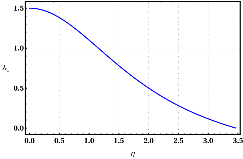
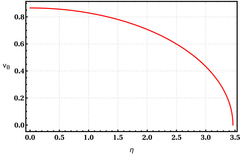
Figure 3: Variation of the Lyapunov exponent ($\lambda_{L}$) and butterfly velocity ($v_{B}$) with respect to the non-conformal parameter $\eta$, with $d=3$ and $r_{+}=1$ (for $\lambda_{L}$).

Finally, by using the metric components (on the horizon), eq.(34) leads us to the following familiar form of the scrambling time

$$t_{*}\approx\left(\frac{\beta}{2\pi}\right)\log(S_{\mathrm{BH}})$$ (39)

where the expression for $\beta$ is given in eq.(16) and the Bekenstein-Hawking entropy of the nonconformal black brane has the form $S_{\mathrm{BH}}=\frac{r_{+}^{p(d-1)}}{4}$ .

4 Two-sided mutual information and entanglement velocity

In this section, we compute the mutual information (MI) between the two decoupled quantum mechanical systems existing on both left and right asymptotic boundaries of the two-sided black hole geometry. Further, we do this for both unperturbed and perturbed geometries in order to quantify the effect of shock wave on MI.

4.1 Two-sided mutual information for the unperturbed geometry

Firstly, we holographically compute the two-sided MI in absence of the shock wave. In order to do this, we consider two strip-like, identical subsystems of length $l$, namely, $A$ and $B$ which belongs to the left and right asymptotic boundaries respectively. The geometry of these strip subsystems ($A$ and $B$) can be specified as $-\frac{l}{2}\leq x_{1}(r)\leq\frac{l}{2}$ and $-\frac{L}{2}\leq x^{m}\leq\frac{L}{2}$ for $m=2,..,d-1$. As mentioned previously, the expression for MI is given by eq.(5). This in turn means that one needs to compute the von Neumann entropies associated to subsystem $A$, $B$ and $A\cup B$. In the gauge/gravity set up, one can holographically do this by incorporating the HRT proposal Ryu:2006bv ; Ryu:2006ef ; Hubeny:2007xt which states that the von Neumann entropy of a subsystem (namely $A$) can be computed with the help of the extremal surface with minimal area $\gamma_{A}$. By incorporating this proposal, one can obtain the following result Saha:2020fon

$$S_{\mathrm{vn}}(A)=S_{\mathrm{vn}}(B)=\frac{2L^{d-2}}{4}\int_{r_{t}}^{\infty}\frac{r^{p(d-3)}dr}{\sqrt{f(r)}\sqrt{1-\left(\frac{r_{t}}{r}\right)^{2p(d-1)}}}$$ (40)

where $r_{t}$ is the turning point of the static minimal surface of interest. On the other hand, the relation between subsystem size $l$ and the turning point $r_{t}$ stands to be

$$l=2\int_{r_{t}}^{\infty}\frac{dr}{r^{2p}\sqrt{f(r)}\sqrt{\left(\frac{r}{r_{t}}\right)^{2p}-1}}~{}.$$ (41)

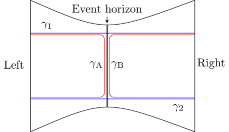
Figure 4: Schematic representation of the two-sided eternal black hole geometry in absence of the shock wave. Here, $\gamma_{A}$ and $\gamma_{B}$ (in red) are Ryu-Takayanagi surfaces associated to subsystem $A$ and $B$. $\gamma_{1}$ and $\gamma_{2}$ (in blue) leads to the extremal surface $\gamma_{\mathrm{wormhole}}=\gamma_{1}\cup\gamma_{2}$ which connects the two decoupled boundaries (right and left).

In case of $S_{\mathrm{vn}}(A\cup B)$, one proceeds with the surface $\gamma_{\mathrm{wormhole}}=\gamma_{1}\cup\gamma_{2}$ which bifurcates the event horizon in order to connect both asymptotic boundaries. This is basically a non-traversable wormhole geometry which induces entanglement between the two decoupled theories (at right and left asymptotic boundaries of the geometry). It is to be mentioned that $\gamma_{1}$ corresponds to the $x_{1}=-\frac{l}{2}$ hyperplane and $\gamma_{2}$ corresponds to the $x_{1}=\frac{l}{2}$ hyperplane. If we consider the area of a single surface (with such properties), then symmetry tells us that total area will be four times of that surface (a graphical representation of the set up has been provided in Fig.(4)). This leads to the following expression

$$S_{\mathrm{vn}}(A\cup B)\equiv\frac{\mathrm{Area}(\gamma_{\mathrm{wormhole}})}{4}=\frac{4L^{d-2}}{4}\int_{r_{+}}^{\infty}\frac{r^{p(d-3)}dr}{\sqrt{f(r)}}~{}.$$ (42)

We now substitute the expressions from eq.(40) and eq.(42) in eq.(5) and obtain the following form of two-sided MI (in the absence of shock wave)

$$I(A:B)=L^{d-2}\left[\int_{r_{t}}^{\infty}\frac{r^{p(d-3)}dr}{\sqrt{f(r)}\sqrt{1-\left(\frac{r_{t}}{r}\right)^{2p(d-1)}}}-\int_{r_{+}}^{\infty}\frac{r^{p(d-3)}dr}{\sqrt{f(r)}}\right]~{}.$$ (43)

The above expression represents the mutual correlation between the two decoupled theories living at the right and left asymptotic boundaries of the two-sided non-conformal black brane geometry (given in eq.(14)). It can be observed that the expression is written in terms of the bulk coordinate $r$ and one can represent it in terms of the boundary coordinate (subsystem size $l$) with the help of eq.(41).

4.2 Two-sided mutual information for the shock wave geometry

We now proceed to compute the expression of $I(A:B)$ in presence of the shock wave modification of the original geometry. In order to do this, we follow the computational procedure shown in Leichenauer:2014nxa . In this work, we are considering a homogeneous shock wave which is introducing deformation to the $v$-coordinate which in turn stretches the wormhole geometry. This in turn means that only the term $S_{\mathrm{vn}}(A:B)$ will get effected due to the presence of shock wave as it is the only term in eq.(5) which depends on the wormhole geometry. On the other hand, $S_{\mathrm{vn}}(A)$ and $S_{\mathrm{vn}}(B)$ will remain unchanged as their associated extremal surfaces do not bifurcate the event horizon Hubeny:2012ry . This can be graphically represented by a schematic diagram which has been provided in Fig.(5).

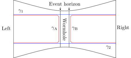
Figure 5: Schematic representation of the shock wave geometry. In presence of shock wave, only the extremal surface $\gamma_{\mathrm{wormhole}}=\gamma_{1}\cup\gamma_{2}$ is getting affected.

Keeping this in mind, for the shock wave geometry, one can write down the following expression

$$I(A:B;\alpha) = S_{\mathrm{vn}}(A)+S_{\mathrm{vn}}(B)-S_{\mathrm{vn}}(A\cup B;\alpha)$$ (44)

$$= S_{\mathrm{vn}}(A)+S_{\mathrm{vn}}(B)-S_{\mathrm{vn}}(A\cup B;\alpha=0)-\left(S_{\mathrm{vn}}(A\cup B;\alpha)-S_{\mathrm{vn}}(A\cup B;\alpha=0)\right)$$

$$= I(A:B;\alpha=0)-S^{\mathrm{reg}}_{\mathrm{vn}}(A\cup B;\alpha)$$

where $I(A:B;\alpha=0)$ is given in eq.(43) and $S^{\mathrm{reg}}_{\mathrm{vn}}(A\cup B;\alpha)$ represents a regularized expression for von Neumann entropy which is free of the universal divergence term. Furthermore, in the above computation we have also introduced $S_{\mathrm{vn}}(A\cup B;\alpha=0)$, which we have already computed in eq.(42). The expression given in eq.(44) in turn means that we need to compute only the term $S^{\mathrm{reg}}_{\mathrm{vn}}(A\cup B;\alpha)$. In order to compute $S_{\mathrm{vn}}(A\cup B;\alpha)$ we first specify the parametrization of the corresponding HRT surfaces $r=r(t),x_{1}=\pm\frac{l}{2}$ and $-\frac{L}{2}\leq x^{m}\leq\frac{L}{2}$ for $m=2,..,d-1$. This leads to the corresponding area functional

$$\mathrm{Area}(\gamma^{SW}_{\mathrm{wormhole}})=L^{d-2}\int r^{p(d-1)}\sqrt{-f(r)+\frac{\dot{r}^{2}}{r^{4p}f(r)}}dt~{}.$$ (45)

From the above action one can point out the relevant Lagrangian density. This reads

$$\mathcal{L}(r,\dot{r},t)=L^{d-2}r^{p(d-1)}\sqrt{-f(r)+\frac{\dot{r}^{2}}{r^{4p}f(r)}}~{}.$$ (46)

The corresponding Hamiltonian density can easily be obtained and it can be observed that it does not have an explicit time-dependency. This in turn gives us the following conserved quantity

$$\mathcal{C}=-r_{0}^{p(d-1)}\sqrt{-f(r_{0})}$$ (47)

which is associated to the condition $\dot{r}|_{r=r_{0}}=0$. The on-shell area functional reads

$$\mathrm{Area}(\gamma^{SW}_{\mathrm{wormhole}})=L^{d-1}\int\frac{r^{p(d-3)}dr}{\sqrt{f(r)-\left(\frac{r_{0}}{r}\right)^{2p(d-1)}f(r_{0})}}~{}.$$ (48)

On the other hand, the time-coordinate can be represented in the following way

$$t(r)=\pm\int\frac{dr}{r^{2p}f(r)\sqrt{1-\left(\frac{r}{r_{0}}\right)^{2p(d-1)}\frac{f(r)}{f(r_{0})}}}~{}.$$ (49)

We now proceed to specify the domain of integration for the above expressions. The domain of interest can be divided into three segments which has been pointed out in Fig.(6). It can be observed that segment II and segment III has the same area. Keeping these observations in mind, we write down the following form

$$S_{\mathrm{vn}}(A\cup B;\alpha)=\frac{4L^{d-2}}{4}\left[\int_{r_{+}}^{\infty}\frac{r^{p(d-3)}dr}{\sqrt{f(r)-\left(\frac{r_{0}}{r}\right)^{2p(d-1)}f(r_{0})}}+2\int_{r_{0}}^{r_{+}}\frac{r^{p(d-3)}dr}{\sqrt{f(r)-\left(\frac{r_{0}}{r}\right)^{2p(d-1)}f(r_{0})}}\right]~{}.$$

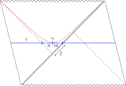
Figure 6: Deformation of the extremal surface $\gamma_{\mathrm{wormhole}}$ (in blue) due to the shock wave. We have divided the left half of the surface into three parts segment $\mathrm{I}$ which spans from the boundary ($r=\infty$) to the horizon $r_{+}$ and both segment $\mathrm{II}$ and segment $\mathrm{III}$ spans from $r_{0}$ to the horizon $r_{+}$. Thus, segment $\mathrm{II}$ and segment $\mathrm{III}$ have same area.

With above result in hand, we now make use of the expression of $S_{\mathrm{vn}}(A\cup B;\alpha=0)$ (given in eq.(42)) in order to obtain the regularized version of $S_{\mathrm{vn}}(A\cup B;\alpha)$. This reads

$$S^{\mathrm{reg}}_{\mathrm{vn}}(A\cup B;\alpha) = S_{\mathrm{vn}}(A\cup B;\alpha)-S_{\mathrm{vn}}(A\cup B;\alpha=0)$$ (51)

$$= \frac{4L^{d-2}}{4}\Bigg{[}\int_{r_{+}}^{\infty}r^{p(d-3)}\left(\frac{1}{\sqrt{f(r)-\left(\frac{r_{0}}{r}\right)^{2p(d-1)}f(r_{0})}}-\frac{1}{\sqrt{f(r)}}\right)dr$$

$$+ 2\int_{r_{0}}^{r_{+}}\frac{r^{p(d-3)}dr}{\sqrt{f(r)-\left(\frac{r_{0}}{r}\right)^{2p(d-1)}f(r_{0})}}\Bigg{]}~{}.$$

As we have explained in eq.(44), the above expression of $S^{\mathrm{reg}}_{\mathrm{vn}}(A\cup B;\alpha)$ along with the expression of $I(A:B;\alpha=0)$ (given in eq.(43)) leads us to the desired result of $I(A:B;\alpha)$. It is to be observed from the above given expression of $S^{\mathrm{reg}}_{\mathrm{vn}}(A\cup B;\alpha)$ that it is a function of $r_{0}$. This in turn means that we need to find the relation between $\alpha$ (shock wave parameter) and $r_{0}$ so that we can depict the variation of $S^{\mathrm{reg}}_{\mathrm{vn}}(A\cup B;\alpha)$ with respect to the shock wave parameter. In order to do this, we follow the approach given in Leichenauer:2014nxa . As we have mentioned earlier, our domain of interest can be divided into three segments, namely, $\mathrm{I}$, $\mathrm{II}$ and $\mathrm{III}$. In terms of the Kruskal coordinates, the segment $\mathrm{I}$ connects $(u,v)=(1,-1)$ (boundary) to $(u,v)=(u_{1},0)$ (horizon). Segment $\mathrm{II}$ connects $(u,v)=(u_{1},0)$ (horizon) to the point $r_{0}$ which is at $(u,v)=(u_{2},v_{2})$ and segment $\mathrm{III}$ connects $(u,v)=(u_{2},v_{2})$ to $(u,v)=(0,\alpha/2)$. Keeping these coordinates in mind and by using the Kruskal coordinates, one can show the following relations

$$u_{1}^{2} = \exp(\frac{4\pi}{\beta}\int_{r_{+}}^{\infty}\frac{dr}{r^{2p}f(r)}\left[\frac{1}{\sqrt{1-\left(\frac{r}{r_{0}}\right)^{2p(d-1)}\frac{f(r)}{f(r_{0})}}}-1\right])$$

$$u_{2}^{2} = \exp(\frac{4\pi}{\beta}\int_{r_{0}}^{r_{+}}\frac{dr}{r^{2p}f(r)}\left[\frac{1}{\sqrt{1-\left(\frac{r}{r_{0}}\right)^{2p(d-1)}\frac{f(r)}{f(r_{0})}}}-1\right])$$

$$v_{2} = \frac{1}{u_{2}}\exp(-\frac{4\pi}{\beta}\int_{r_{0}}^{\bar{r}}\frac{dr}{r^{2p}f(r)})~{}.$$ (52)

In the last of the above equations, $\bar{r}$ point resides inside the horizon at which $r_{*}=0$. From segment $\mathrm{III}$, one can show the following relation by incorporating the variation in the $v$-coordinate

$$\frac{\alpha^{2}}{4v_{2}^{2}}=\exp(\frac{4\pi}{\beta}\int_{r_{+}}^{r_{0}}\frac{dr}{r^{2p}f(r)}\left[\frac{1}{\sqrt{1-\left(\frac{r}{r_{0}}\right)^{2p(d-1)}\frac{f(r)}{f(r_{0})}}}-1\right])=\frac{u_{1}^{2}}{u_{2}^{2}}~{}.$$ (53)

Now, by using the relation given eq.(4.2) in the above equation and after some simplifications, one obtains the following relation

$$\alpha(r_{0})=2\exp(\xi_{I}+\xi_{II}+\xi_{III})$$ (54)

where

$$\xi_{I} = \frac{4\pi}{\beta}\int_{\bar{r}}^{r_{0}}\frac{dr}{r^{2p}f(r)}$$

$$\xi_{II} = \frac{2\pi}{\beta}\int_{r_{+}}^{\infty}\frac{dr}{r^{2p}f(r)}\left[1-\frac{1}{\sqrt{1-\left(\frac{r}{r_{0}}\right)^{2p(d-1)}\frac{f(r)}{f(r_{0})}}}\right]$$

$$\xi_{III} = \frac{4\pi}{\beta}\int_{r_{0}}^{r_{+}}\frac{dr}{r^{2p}f(r)}\left[1-\frac{1}{\sqrt{1-\left(\frac{r}{r_{0}}\right)^{2p(d-1)}\frac{f(r)}{f(r_{0})}}}\right]~{}.$$ (55)

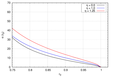
Figure 7: Behaviour of the shock wave parameter $\alpha(r_{0})$ with respect to the turning point $r_{0}$. We have set $r_{+}=1$ and $d=3$.

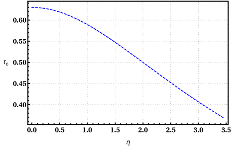
Figure 8: Effect of non-conformal parameter $\eta$ on $r_{c}$. We have set $r_{+}=1$ and $d=3$.

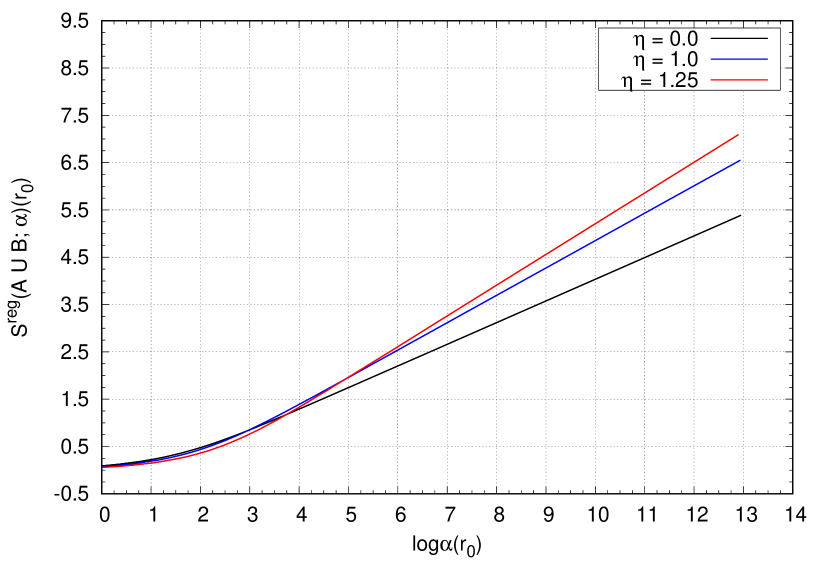
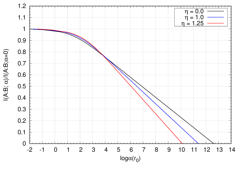
Figure 9: The left plot represents the behaviour of $S^{\mathrm{reg}}_{\mathrm{vn}}(A\cup B;\alpha)$ with respect to $\log\alpha$. The right plot captures the behaviour of two-sided mutual information in presence of the shock wave. Here, we have set $r_{+}=1$, $L=1$ and $d=3$.

In Fig.(7), we have graphically represented the relation given in eq.(54) where we have set $r_{+}=1$. We observe that for a fixed value of $r_{0}$, $\alpha(r_{0})$ increases with the increase in the value of the non-conformal parameter $\eta$. One can also note that in the limit $r_{0}\rightarrow r_{+}$, the shock wave parameter $\alpha(r_{0})$ vanishes and for a critical value of $r_{0}$, namely, at $r_{0}=r_{c}$ it diverges. In fact, it can also be observed that at this particular value $r_{0}=r_{c}$, only $\xi_{III}$ diverges which depicts the fact that in the limit $r_{0}\rightarrow r_{c}$, $\xi_{III}$ is the dominating piece in the expression of $\alpha(r_{0})$ (given in eq.(54).) One can derive the value of $r_{c}$ by performing a Taylor expansion of the integrand of $\xi_{III}$ around $r_{0}\approx r_{c}$ and equating the coefficient of $(r_{0}-r_{c})$ to zero Jahnke:2017iwi ; Fischler:2018kwt ; Avila:2018sqf . We shall follow this approach to derive the explicit expression of $r_{c}$. Firstly, the expression of $\xi_{III}$ around $r\approx r_{0}$ has the following form

$$\xi_{III}\approx\frac{4\pi}{\beta}\int_{r_{0}}^{r_{+}}\frac{dr}{r_{0}^{2p}f(r_{0})}\left[1-\frac{1}{\sqrt{\left(-\frac{2p(d-1)}{r_{0}}-\frac{f^{\prime}(r_{0})}{f(r_{0})}\right)(r-r_{0})}}\right]~{}.$$ (56)

The above expression diverges at $-\frac{2p(d-1)}{r_{0}}-\frac{f^{\prime}(r_{0})}{f(r_{0})}|_{r_{0}=r_{c}}=0$. By solving this one obtains

$$r_{c}=r_{+}\left[1-\frac{c}{2p(d-1)}\right]^{\frac{1}{c}}~{}.$$ (57)

In the limit $\eta\rightarrow 0$, one obtains the conformal result $r_{c}=r_{+}\left[\frac{d-2}{2(d-1)}\right]^{\frac{1}{d}}$ Leichenauer:2014nxa . In Fig.(8), we have tried to capture the effect of non-conformality on $r_{c}$. We observe that non-conformality decreases the value of $r_{c}$ which implies the fact that non-conformality helps to probe the black hole interior further. In Fig.(9), the behaviour of $S^{\mathrm{reg}}_{\mathrm{vn}}(A\cup B;\alpha)$ and $\frac{I(A:B;\alpha)}{I(A:B;\alpha=0)}=1-\frac{S^{\mathrm{reg}}_{\mathrm{vn}}(A\cup B;\alpha)}{I(A:B;\alpha=0)}$ with respect to the logarithm of the shock wave parameter ($\log\alpha$) has been provided. We observe that for a fixed value of $\log\alpha$, $S^{\mathrm{reg}}_{\mathrm{vn}}(A\cup B;\alpha)$ increases with the increase in the value of the non-conformal parameter $\eta$. On the other hand, due to non-cormality, $S^{\mathrm{reg}}_{\mathrm{vn}}(A\cup B;\alpha)$ becomes equal to $I(A:B;\alpha=0)$ (resulting in $\frac{I(A:B;\alpha)}{I(A:B;\alpha=0)}=0$) for a smaller value of $\log\alpha$.

4.3 Entanglement velocity

We now proceed to study the behaviour of $S^{\mathrm{reg}}_{\mathrm{vn}}(A\cup B;\alpha)$ with respect to the time $t$ at which the initial perturbation was added. It can be observed that $S^{\mathrm{reg}}_{\mathrm{vn}}(A\cup B;\alpha)$ grows linearly with respect to $\log\alpha$ which in turn means it grows linearly with respect to $t$ (as $\alpha\approx e^{\frac{2\pi}{\beta}t}$). This can be observed from the left plot of Fig.(9). This linear behaviour of $S^{\mathrm{reg}}_{\mathrm{vn}}(A\cup B;\alpha)$ in turn helps us to quantify the spreading of entanglement in a chaotic system by introducing the entanglement velocity in this set up. In order to capture the behaviour of $S^{\mathrm{reg}}_{\mathrm{vn}}(A\cup B;\alpha)$ around $r_{0}\approx r_{c}$, we first expand $S^{\mathrm{reg}}_{\mathrm{vn}}(A\cup B;\alpha)$ upto linear order in $(r-r_{0})$. This leads to the following form

$$S^{\mathrm{reg}}_{\mathrm{vn}}(A\cup B;\alpha) \approx 2L^{d-2}\sqrt{-f(r_{0})}r_{0}^{p(d-1)}\int_{r_{0}}^{r_{+}}\frac{dr}{r_{0}^{2p}f(r_{0})\sqrt{\left(-\frac{2p(d-1)}{r_{0}}-\frac{f^{\prime}(r_{0})}{f(r_{0})}\right)(r-r_{0})}}$$ (58)

$$= 2L^{d-2}\sqrt{-f(r_{0})}r_{0}^{p(d-1)}\int_{r_{0}}^{r_{+}}\frac{dr}{r_{0}^{2p}f(r_{0})}\left[1-\frac{1}{\sqrt{\left(-\frac{2p(d-1)}{r_{0}}-\frac{f^{\prime}(r_{0})}{f(r_{0})}\right)(r-r_{0})}}\right]$$

$$- 2L^{d-2}\sqrt{-f(r_{0})}r_{0}^{p(d-1)}\int_{r_{0}}^{r_{+}}\frac{dr}{r_{0}^{2p}f(r_{0})}~{}.$$

Now, by using the relation given in eq.(56), we can write down the following form of $S^{\mathrm{reg}}_{\mathrm{vn}}(A\cup B;\alpha)$ and proceed to consider the $r_{0}\rightarrow r_{c}$ limit

$$S^{\mathrm{reg}}_{\mathrm{vn}}(A\cup B;\alpha)\approx 2L^{d-2}\sqrt{-f(r_{0})}r_{0}^{p(d-1)}\left(\frac{\beta}{4\pi}\right)\log\alpha(r_{0})\bigg{|}_{r_{0}=r_{c}}~{}.$$ (59)

Keeping in mind the exponential growth of the given perturbation, that is, $\alpha\sim\exp^{\frac{2\pi t}{\beta}}$, one can write down the following equation Hartman:2013qma ; Liu:2013iza ; Liu:2013qca ; Mezei:2016wfz ; Mezei:2016zxg

$$\frac{dS^{\mathrm{reg}}_{\mathrm{vn}}(A\cup B;\alpha)}{dt} = 2L^{d-2}\sqrt{-f(r_{c})}r_{c}^{p(d-1)}\left(\frac{\beta}{4\pi}\right)\left(\frac{2\pi}{\beta}\right)$$ (60)

$$= 4L^{d-2}\sqrt{-f(r_{c})}\left(\frac{r_{c}}{r_{+}}\right)^{p(d-1)}\left(\frac{r_{+}^{p(d-1)}}{4}\right)$$

$$= s_{th}\mathcal{A}_{\Sigma}v_{en}$$

where $s_{th}$ is the thermal entropy density $s_{th}=\frac{r_{+}^{p(d-1)}}{4}$, $\mathcal{A}_{\Sigma}=4L^{d-2}$ is the area of the hyperplane and $v_{en}$ is the entanglement velocity which has the following form

$$v_{en}=\left(\frac{r_{c}}{r_{+}}\right)^{p(d-1)}\sqrt{-f(r_{c})}~{}.$$ (61)

By using the explicit value of $r_{c}$ (given in eq.(57)), one can obtain an exact expression for the entanglement velocity. This reads

$$v_{en}=\left[1-\frac{c}{2p(d-1)}\right]^{\frac{p(d-1)}{c}}\sqrt{\frac{c}{2p(d-1)-c}}~{}.$$ (62)

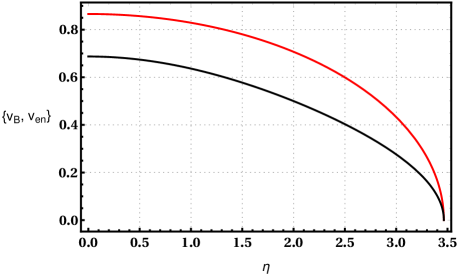
Figure 10: Comparison between the variations of the butterfly velocity (red curve) and entanglement velocity (black curve) with respect to the non-conformal parameter $\eta$.

In the limit $\eta\rightarrow 0$, one obtains the standard conformal result (result for SAdS_d+1). This reads Hartman:2013qma

$$v_{en}=\frac{\sqrt{d}(d-2)^{\frac{1}{2}-\frac{1}{d}}}{[2(d-1)]^{1-\frac{1}{d}}}~{}.$$ (63)

From our obtained result of entanglement velocity (given in eq.(62)), we observe that similar to the butterfly velocity and Lyapunov exponent, it also decreases with the increase in the value of the non-conformal parameter $\eta$. Furthermore, $v_{en}$ also vanishes for $\eta=\sqrt{\frac{8d}{(d-1)}}$ representing the complete disruption of quantum entanglement. We have represented our observations graphically in Fig.(10). Fig.(10) also reveals that in the presence of non-conformality, entanglement velocity still satisfies the property $v_{en}\leq v_{B}$. Further, both of these velocities are always less than the speed of light (as speed of light $v_{c}=1$).

5 Pole-skipping analysis: Lyapunov exponent and Butterfly velocity

In this section, we will point out the special points, known as the pole-skipping points, in the complex $(\omega,k)$ plane at which the near-horizon solution of the bulk field is ill-defined which leads to the non-unique nature of the corresponding retarded Green’s function. As mentioned earlier, the location of these points in the complex $(\omega,k)$ (upper half or lower half) depends on the spin $s$ of the bulk field. As we have already shown in eq.(10), only the upper half pole-skipping points are related to the Lyapunov exponent and the butterfly velocity. In this section, we will also verify these statements by considering two different kinds of field perturbation, namely, metric perturbation and scalar field perturbation. As we are interested in the near horizon analysis of the bulk field equation of motion, we recast the bulk metric (given in eq.(14)) in the ingoing Eddington-Finkelstein coordinate system

$$v=t+r_{*}~{}.$$ (64)

In the above coordinate system, the bulk metric takes the following form

$$ds^{2}=-r^{2p}f(r)dv^{2}+2dvdr+h(r)\sum_{i=1}^{d-1}dx_{i}^{2}~{},~{}h(r)=r^{2p}~{}.$$ (65)

On the other hand, we assume the following linear perturbation of the metric and the dilaton field (in the $x_{1}$ direction)

$$\delta g_{\mu\nu}(v,r,x_{1}) = \delta g_{\mu\nu}(r)e^{-i\omega v+ikx_{1}}$$

$$\delta\phi(v,r,x_{1}) = \delta\phi(r)e^{-i\omega v+ikx_{1}}~{}.$$ (66)

In the sound mode, the relevant perturbations are $\delta g_{vv}$, $\delta g_{vr}$, $\delta g_{vx_{1}}$, $\delta g_{rr}$, $\delta g_{rx_{1}}$, $\delta g_{x_{i}x_{i}}$ along with $\delta\phi$ which can couple to any of these metric fluctuations. As the location of the pole-skipping point $(\omega_{*},k_{*})$ depends on the behaviour of the background metric on the horizon, one has to consider the near-horizon behaviour of these perturbations Blake:2018leo ; Blake:2019otz ; Blake:2021hjj . In the near-horizon regime, the perturbations behave in the following way

$$\delta g_{\mu\nu}(r) = \delta g_{\mu\nu}^{(0)}+\delta g_{\mu\nu}^{(1)}(r-r_{+})+\mathcal{O}(r-r_{+})^{2}...$$

$$\delta\phi(r) = \delta\phi^{(0)}+\delta\phi^{(1)}(r-r_{+})+\mathcal{O}(r-r_{+})^{2}...~{}.$$ (67)

We now follow the approach given in Blake:2018leo . By substituting the above forms of perturbations in the Einstein field equations (given in eq.(12)) and by considering the near-horizon limit, one observes that the $vv$-component of the Einstein-field equation assumes the following universal form Blake:2018leo

$$\left(-i\frac{(d-1)}{2}\omega h^{\prime}(r_{+})+k^{2}\right)\delta g_{vv}^{(0)}-i(2\pi T_{H}+i\omega)\left(\omega\delta g_{x_{i}x_{i}}^{(0)}+2k\delta g_{vx_{1}}^{(0)}\right)=0~{}.$$ (68)

By incorporating the background metric informations from eq.(65), we obtain the following form for the case we have in hand

$$\left(-i\frac{(d-1)}{2}\omega\partial_{r}r^{2p}|_{r=r_{+}}+k^{2}\right)\delta g_{vv}^{(0)}-i(2\pi T_{H}+i\omega)\left(\omega\delta g_{x_{i}x_{i}}^{(0)}+2k\delta g_{vx_{1}}^{(0)}\right)=0~{}.$$ (69)

From the above equation, one can easily point out the special values of $\omega$ and $k$ for which the equation gets satisfied. The values of $\omega$ read

$$\omega=i2\pi T_{H}\equiv\omega_{*}~{}.$$ (70)

On the other hand, for $k$, the corresponding special value is given by

$$k = \sqrt{i\frac{(d-1)}{2}\omega_{*}\partial_{r}r^{2p}|_{r=r_{+}}}$$ (71)

$$= i\frac{2\pi T_{H}}{\sqrt{\frac{c}{2p(d-1)}}}$$

$$= k_{*}~{}.$$

We now make use of the relations given in eq.(10) along with the above obtained values of $\omega_{*}$ and $k_{*}$ to obtain the following results

$$\lambda_{L}=\frac{2\pi}{\beta};~{}v_{B}=\sqrt{\frac{c}{2p(d-1)}}\equiv\frac{1}{4}\sqrt{\frac{8d}{d-1}-\eta^{2}}~{}.$$ (72)

The above results agrees perfectly with that obtained from the shock wave analysis (eq.(37)).

5.1 Pole-skipping for higher Matsubara frequencies

In the previous section, we have determined the parameters of quantum chaos from the lowest order values of ($\omega_{*},k_{*}$) which resides in the upper half of the complex ($\omega,k$)-plane. We now move on to compute the higher order values of $(\omega_{*},k_{*})$ by considering scalar field fluctuations in the gravitational background. We start our analysis by considering a minimally coupled massive scalar field $\Psi(v,r,x_{1})$, the equation of motion for which is governed by the following Klein-Gordon (KG) equation

$$\frac{1}{\sqrt{-g}}\partial_{\mu}\left(\sqrt{-g}g^{\mu\nu}\partial_{\nu}\Psi\right)-m^{2}\Psi=0$$ (73)

with the background metric being given by eq.(65). The above equation assumes the following form in the Eddington-Finkelstein coordinate

$$p(d-1)r^{p(d-1)-1}\partial_{v}\Psi+2r^{p(d-1)}\partial_{v}\partial_{r}\Psi+p(d+1)r^{p(d+1)-1}f(r)\partial_{r}\Psi$$

$$+r^{p(d+1)}f^{\prime}(r)\partial_{r}\Psi+r^{p(d+1)}f(r)\partial^{2}_{r}\Psi+r^{p(d-3)}\partial^{2}_{x_{1}}\Psi-r^{p(d-1)}m^{2}\Psi=0~{}.$$ (74)

We now consider the following Fourier decomposition of the massive scalar field

$$\Psi(v,r,x_{1})=\psi(r)e^{-i\omega v+ikx_{1}}~{}.$$ (75)

By substituting eq.(75) in eq.(5.1), we obtain

$$\psi^{\prime\prime}(r)+\Delta_{1}(r)\psi^{\prime}(r)+\Delta_{2}(r)\psi(r)=0$$ (76)

where

$$\Delta_{1}(r) = \frac{r^{2p}f^{\prime}(r)+p(d+1)r^{2p-1}f(r)-2i\omega}{r^{2p}f(r)}$$

$$\Delta_{2}(r) = -\frac{\frac{k^{2}}{r^{2p}}+m^{2}+\frac{i\omega}{r}p(d-1)}{r^{2p}f(r)}~{}.$$ (77)

In order to find out the pole-skipping points, one needs to consider the near-horizon limit. The near-horizon expansion for the scalar field reads $\psi(r)$

$$\psi(r)=\psi_{0}+\psi_{1}(r-r_{+})+\psi_{2}(r-r_{+})^{2}+...~{}.$$ (78)

By substituting the above near-horizon form of $\psi(r)$ in eq.(76) and by equating the coefficients of $(r-r_{+})^{j}$ (for $j=0,1,2..$) to zero, one obtains a set of linear equations which read

$$\chi_{00}\psi_{0}+\chi_{01}\psi_{1} = 0,$$

$$\chi_{10}\psi_{0}+\chi_{11}\psi_{1}+\chi_{12}\psi_{2} = 0,$$

$$\chi_{20}\psi_{0}+\chi_{21}\psi_{1}+\chi_{22}\psi_{2}+\chi_{23}\psi_{3} = 0$$

$$\ ...$$ (79)

where

$$\chi_{00} = -\left(\frac{k^{2}}{r_{+}^{2p}}+m^{2}+\frac{i\omega}{r_{+}}p(d-1)\right)$$

$$\chi_{01} = r_{+}^{2p}f^{\prime}(r_{+})-2i\omega$$

$$\chi_{10} = 0$$

$$\chi_{11} = 2r_{+}^{2p}f^{\prime\prime}(r_{+})+p(d+1)r_{+}^{2p-1}f^{\prime}(r_{+})-\left(\frac{k^{2}}{r_{+}^{2p}}+m^{2}+\frac{i\omega}{r_{+}}p(d-1)\right)$$

$$\chi_{12} = 4r_{+}^{2p}f^{\prime}(r_{+})-4i\omega$$

$$....$$ (80)

The coefficients $\chi_{ij}$ can arranged to form a square a matrix

$$\mathcal{M}=\begin{bmatrix}\chi_{00}&\chi_{01}&0&0&...\\ \chi_{10}&\chi_{11}&\chi_{12}&0&...\\ \chi_{20}&\chi_{21}&\chi_{22}&\chi_{23}&...\\ ...&...&...&...\\ \end{bmatrix}$$

The pole-skipping points are to be obtained by simultaneously solving the equations Blake:2019otz

$$\chi_{n-1~{}n}=0;~{}\det(\mathcal{M})=0~{}.$$ (81)

We now provide the locations of some of these pole-skipping points. These read

$$\omega_{1}=-i2\pi T_{H}; ~{}k_{1}=-i\frac{2\pi T_{H}}{\sqrt{\frac{c}{2p(d-1)}}}\left[1+\frac{m^{2}}{2p(d-1)\pi}\left(\frac{4\pi}{c}\right)^{\frac{1}{(2p-1)}}T_{H}^{\frac{2-2p}{2p-1}}\right]^{1/2},$$

$$\omega_{2}=-i4\pi T_{H}; k_{2}=-i\frac{4\pi T_{H}}{\sqrt{\frac{c}{p(d-1)+2(c+1)-p(d+1)}}}$$

$$\times\left[1+\frac{m^{2}}{\left(4\pi\right)^{2}}\left(\frac{c}{p(d-1)+2(c+1)-p(d+1)}\right)\left(\frac{4\pi}{c}\right)^{\frac{2p}{2p-1}}T_{H}^{\frac{2-2p}{2p-1}}\right]^{1/2}$$

$$....$$ (83)

6 Conclusion

We now summarize our findings. In this work, we have holographically studied the behaviour of the parameters of chaos in presence of non-conformality. By incorporating the gauge/gravity framework, we have introduced the two-sided black hole geometry which is the well-known dual description for the thermofield doublet state. This realization helps us to quantify the effects of chaos on the correlation which exists between the right and left boundary theories of the two-sided geometry. The non-conformality in the boundary theories has been holographically introduced by considering the black brane solution of the Einstein-dilaton theory where the dilaton potential is of Liouville type. The asymptote of the black brane geometry is a warped geometry instead of a pure AdS geometry. This implies that the boundary theory is nonconformal, however, it is relativistic as the Poincare symmetry is still restored. The black brane solution is associated with a parameter $\eta$ which characterizes the deviation from conformality as in the limit $\eta\rightarrow 0$, one obtains the usual Schwarzschild black brane solution. In order to keep things general, we have considered the gravitational theory is of $(d+1)$-dimensional which in turn means the boundary theories are $d$-dimensional. In order to compute the parameters of chaos which are Lyapunov exponent and the butterfly velocity, we obtain the shock wave geometry corresponding to the black brane solution under consideration. The shock wave geometry arises due to the introduction of a tiny pulse of energy in the geometry (or in dual sense, adding of perturbation at the boundary theory). Due to presence of event horizon, the energy of the pulse gets blue-shifted resulting in a non-trivial modification to the original geometry. The obtained results for the Lypunov exponent and butterfly velocity from the shock wave analysis reveal some interesting observations. We observe that both of these quantities decreases with increase in the value of the nonconformal parameter $\eta$ and finally both of these quantities vanishes for $\eta=\sqrt{\frac{8d}{d-1}}$, representing Lyapunov stability for the system. This particular value of $\eta$ matches perfectly with the previously known upper bound of $\eta$, known as the Gubser bound. Our results also confirm the value of this bound from the point of view of chaos. Our results also indicate that non-conformality helps to suppress the chaotic nature for a system.
On the other hand, it is a well-known fact that the left and right boundary theories of a two-sided geometry share a non-vanishing quantum correlation between them which can be characterized by the mutual information between the mentioned two sides. In order to observe the effects of chaos and non-conformality, we compute the two-sided mutual information both in presence and absence of the shock wave. We observe that non-conformality increases the existing entanglement between the boundary theories, namely, $A$ and $B$. This can be understood from the behaviour of $S^{\mathrm{reg}}_{\mathrm{vn}}(A\cup B;\alpha)$ as its value increases with the increase in the value of $\eta$ (for a fixed value of the shock wave parameter $\log\alpha$). We also note that there is critical value for $r_{0}$, namely, $r_{c}$ at which the shock wave parameter diverges. Furthermore, an increase in value of $\eta$ decreases the value of $r_{c}$. This in turn means that the presence of non-conformality helps us to probe further the black hole interior as the point $r_{0}$ resides inside the black hole interior. In order to understand the spreading of entanglement for a chaotic system, we proceed to compute the entanglement velocity. We observe that similar to the butterfly velocity, this quantity also decreases with the increase in non-conformality, maintaining the bound $v_{B}<v_{en}$.
Finally, we once again obtain the Lyapunov exponent and butterfly velocity from the lowest pole-skipping points in the upper half of the complex-$(\omega,k)$ plane. We observe that the obtained results matches perfectly with that obtained from the shock wave analysis. We also compute higher order pole-skipping points (in the lower half of the complex-$(\omega,k)$ plane) by considering scalar field fluctuation in the bulk geometry.

7 Acknowledgements

AS would like to acknowledge SNBNCBS, Kolkata for the post doctoral fellowship.

References

- (1) M. Cencini, F. Cecconi and A. Vulpiani, Chaos, WORLD SCIENTIFIC (2009), 10.1142/7351, [https://www.worldscientific.com/doi/pdf/10.1142/7351].
- (2) D. Ullmo and S. Tomsovic, Introduction to quantum chaos, 2014, http://www.lptms.u-psud.fr/membres/ullmo/Articles/eolss-ullmo-tomsovic.pdf (2014) .
- (3) A.I. Larkin and Y.N. Ovchinnikov, Quasiclassical method in the theory of superconductivity, Journal of Experimental and Theoretical Physics (1969) .
- (4) S.H. Shenker and D. Stanford, Black holes and the butterfly effect, JHEP 03 (2014) 067 [1306.0622].
- (5) D.A. Roberts and B. Swingle, Lieb-Robinson Bound and the Butterfly Effect in Quantum Field Theories, Phys. Rev. Lett. 117 (2016) 091602 [1603.09298].
- (6) E.H. Lieb and D.W. Robinson, The finite group velocity of quantum spin systems, Commun. Math. Phys. 28 (1972) 251.
- (7) D. Stanford, Many-body chaos at weak coupling, JHEP 10 (2016) 009 [1512.07687].
- (8) J. Maldacena, S.H. Shenker and D. Stanford, A bound on chaos, JHEP 08 (2016) 106 [1503.01409].
- (9) V. Jahnke, Recent developments in the holographic description of quantum chaos, Adv. High Energy Phys. 2019 (2019) 9632708 [1811.06949].
- (10) Y. Sekino and L. Susskind, Fast Scramblers, JHEP 10 (2008) 065 [0808.2096].
- (11) N. Lashkari, D. Stanford, M. Hastings, T. Osborne and P. Hayden, Towards the Fast Scrambling Conjecture, JHEP 04 (2013) 022 [1111.6580].
- (12) J.M. Maldacena, The Large N limit of superconformal field theories and supergravity, Adv. Theor. Math. Phys. 2 (1998) 231 [hep-th/9711200].
- (13) S.S. Gubser, I.R. Klebanov and A.M. Polyakov, Gauge theory correlators from noncritical string theory, Phys. Lett. B 428 (1998) 105 [hep-th/9802109].
- (14) E. Witten, Anti-de Sitter space and holography, Adv. Theor. Math. Phys. 2 (1998) 253 [hep-th/9802150].
- (15) J.M. Maldacena, Eternal black holes in anti-de Sitter, JHEP 04 (2003) 021 [hep-th/0106112].
- (16) M.M. Wolf, F. Verstraete, M.B. Hastings and J.I. Cirac, Area Laws in Quantum Systems: Mutual Information and Correlations, Phys. Rev. Lett. 100 (2008) 070502 [0704.3906].
- (17) I.A. Morrison and M.M. Roberts, Mutual information between thermo-field doubles and disconnected holographic boundaries, JHEP 07 (2013) 081 [1211.2887].
- (18) W. Fischler, A. Kundu and S. Kundu, Holographic Mutual Information at Finite Temperature, Phys. Rev. D 87 (2013) 126012 [1212.4764].
- (19) T. Dray and G. ’t Hooft, The Gravitational Shock Wave of a Massless Particle, Nucl. Phys. B 253 (1985) 173.
- (20) K. Sfetsos, On gravitational shock waves in curved space-times, Nucl. Phys. B 436 (1995) 721 [hep-th/9408169].
- (21) S. Leichenauer, Disrupting Entanglement of Black Holes, Phys. Rev. D 90 (2014) 046009 [1405.7365].
- (22) N. Sircar, J. Sonnenschein and W. Tangarife, Extending the scope of holographic mutual information and chaotic behavior, JHEP 05 (2016) 091 [1602.07307].
- (23) V. Jahnke, Delocalizing entanglement of anisotropic black branes, JHEP 01 (2018) 102 [1708.07243].
- (24) W.-H. Huang, Butterfly Velocity in Quadratic Gravity, Class. Quant. Grav. 35 (2018) 195004 [1804.05527].
- (25) D. Ávila, V. Jahnke and L. Patiño, Chaos, Diffusivity, and Spreading of Entanglement in Magnetic Branes, and the Strengthening of the Internal Interaction, JHEP 09 (2018) 131 [1805.05351].
- (26) W. Fischler, V. Jahnke and J.F. Pedraza, Chaos and entanglement spreading in a non-commutative gauge theory, JHEP 11 (2018) 072 [1808.10050].
- (27) D.S. Ageev, Butterflies dragging the jets: on the chaotic nature of holographic QCD, 2105.04589.
- (28) S. Mahish and K. Sil, Quantum information scrambling and quantum chaos in little string theory, JHEP 08 (2022) 041 [2202.05865].
- (29) S. Chakrabortty, H. Hoshino, S. Pant and K. Sil, A holographic study of the characteristics of chaos and correlation in the presence of backreaction, Phys. Lett. B 838 (2023) 137749 [2206.12555].
- (30) T. Hartman and J. Maldacena, Time Evolution of Entanglement Entropy from Black Hole Interiors, JHEP 05 (2013) 014 [1303.1080].
- (31) M. Mezei, On entanglement spreading from holography, JHEP 05 (2017) 064 [1612.00082].
- (32) P. Calabrese and J.L. Cardy, Evolution of entanglement entropy in one-dimensional systems, J. Stat. Mech. 0504 (2005) P04010 [cond-mat/0503393].
- (33) J.S. Cotler, M.P. Hertzberg, M. Mezei and M.T. Mueller, Entanglement Growth after a Global Quench in Free Scalar Field Theory, JHEP 11 (2016) 166 [1609.00872].
- (34) H. Liu and S.J. Suh, Entanglement Tsunami: Universal Scaling in Holographic Thermalization, Phys. Rev. Lett. 112 (2014) 011601 [1305.7244].
- (35) H. Liu and S.J. Suh, Entanglement growth during thermalization in holographic systems, Phys. Rev. D 89 (2014) 066012 [1311.1200].
- (36) X.-L. Qi and Z. Yang, Butterfly velocity and bulk causal structure, 1705.01728.
- (37) M. Mezei and D. Stanford, On entanglement spreading in chaotic systems, JHEP 05 (2017) 065 [1608.05101].
- (38) M. Blake, R.A. Davison, S. Grozdanov and H. Liu, Many-body chaos and energy dynamics in holography, JHEP 10 (2018) 035 [1809.01169].
- (39) S. Grozdanov, On the connection between hydrodynamics and quantum chaos in holographic theories with stringy corrections, JHEP 01 (2019) 048 [1811.09641].
- (40) M. Blake, R.A. Davison and D. Vegh, Horizon constraints on holographic Green’s functions, JHEP 01 (2020) 077 [1904.12883].
- (41) M. Natsuume, AdS/CFT Duality User Guide, Springer Tokyo (2015), 10.1007/978-4-431-55441-7.
- (42) H. Năstase, Introduction to the AdS/CFT Correspondence, Cambridge University Press (2015), 10.1017/CBO9781316090954.
- (43) M. Natsuume and T. Okamura, Holographic chaos, pole-skipping, and regularity, PTEP 2020 (2020) 013B07 [1905.12014].
- (44) M. Natsuume and T. Okamura, Nonuniqueness of Green’s functions at special points, JHEP 12 (2019) 139 [1905.12015].
- (45) N. Ceplak, K. Ramdial and D. Vegh, Fermionic pole-skipping in holography, JHEP 07 (2020) 203 [1910.02975].
- (46) N. Ceplak and D. Vegh, Pole-skipping and Rarita-Schwinger fields, Phys. Rev. D 103 (2021) 106009 [2101.01490].
- (47) D. Wang and Z.-Y. Wang, Pole Skipping in Holographic Theories with Bosonic Fields, Phys. Rev. Lett. 129 (2022) 231603 [2208.01047].
- (48) M. Blake, H. Lee and H. Liu, A quantum hydrodynamical description for scrambling and many-body chaos, JHEP 10 (2018) 127 [1801.00010].
- (49) M. Natsuume and T. Okamura, Pole-skipping with finite-coupling corrections, Phys. Rev. D 100 (2019) 126012 [1909.09168].
- (50) N. Abbasi and J. Tabatabaei, Quantum chaos, pole-skipping and hydrodynamics in a holographic system with chiral anomaly, JHEP 03 (2020) 050 [1910.13696].
- (51) Y. Ahn, V. Jahnke, H.-S. Jeong, K.-Y. Kim, K.-S. Lee and M. Nishida, Pole-skipping of scalar and vector fields in hyperbolic space: conformal blocks and holography, JHEP 09 (2020) 111 [2006.00974].
- (52) Y. Ahn, V. Jahnke, H.-S. Jeong, K.-Y. Kim, K.-S. Lee and M. Nishida, Classifying pole-skipping points, JHEP 03 (2021) 175 [2010.16166].
- (53) K.-Y. Kim, K.-S. Lee and M. Nishida, Holographic scalar and vector exchange in OTOCs and pole-skipping phenomena, JHEP 04 (2021) 092 [2011.13716].
- (54) M. Natsuume and T. Okamura, Pole-skipping and zero temperature, Phys. Rev. D 103 (2021) 066017 [2011.10093].
- (55) N. Abbasi and M. Kaminski, Constraints on quasinormal modes and bounds for critical points from pole-skipping, JHEP 03 (2021) 265 [2012.15820].
- (56) C. Choi, M. Mezei and G. Sárosi, Pole skipping away from maximal chaos, 2010.08558.
- (57) D.M. Ramirez, Chaos and pole skipping in CFT2, JHEP 12 (2021) 006 [2009.00500].
- (58) N. Abbasi and S. Tahery, Complexified quasinormal modes and the pole-skipping in a holographic system at finite chemical potential, JHEP 10 (2020) 076 [2007.10024].
- (59) K. Sil, Pole skipping and chaos in anisotropic plasma: a holographic study, JHEP 03 (2021) 232 [2012.07710].
- (60) H. Yuan and X.-H. Ge, Pole-skipping and hydrodynamic analysis in Lifshitz, AdS2 and Rindler geometries, JHEP 06 (2021) 165 [2012.15396].
- (61) M. Blake and R.A. Davison, Chaos and pole-skipping in rotating black holes, JHEP 01 (2022) 013 [2111.11093].
- (62) H. Yuan and X.-H. Ge, Analogue of the pole-skipping phenomenon in acoustic black holes, Eur. Phys. J. C 82 (2022) 167 [2110.08074].
- (63) H. Yuan, X.-H. Ge, K.-Y. Kim, C.-W. Ji and Y. Ahn, Pole-skipping points in 2D gravity and SYK model, JHEP 08 (2023) 157 [2303.04801].
- (64) S. Kulkarni, B.-H. Lee, C. Park and R. Roychowdhury, Non-conformal Hydrodynamics in Einstein-dilaton Theory, JHEP 09 (2012) 004 [1205.3883].
- (65) S. Kulkarni, B.-H. Lee, J.-H. Oh, C. Park and R. Roychowdhury, Transports in non-conformal holographic fluids, JHEP 03 (2013) 149 [1211.5972].
- (66) C. Park, Holographic Aspects of a Relativistic Nonconformal Theory, Adv. High Energy Phys. 2013 (2013) 389541 [1209.0842].
- (67) C. Park, Holographic entanglement entropy in the nonconformal medium, Phys. Rev. D 91 (2015) 126003 [1501.02908].
- (68) C. Charmousis, B. Gouteraux and J. Soda, Einstein-Maxwell-Dilaton theories with a Liouville potential, Phys. Rev. D 80 (2009) 024028 [0905.3337].
- (69) S.S. Gubser, Curvature singularities: The Good, the bad, and the naked, Adv. Theor. Math. Phys. 4 (2000) 679 [hep-th/0002160].
- (70) B. Gouteraux and E. Kiritsis, Generalized Holographic Quantum Criticality at Finite Density, JHEP 12 (2011) 036 [1107.2116].
- (71) A. Saha, S. Gangopadhyay and J.P. Saha, Generalized entanglement temperature and entanglement Smarr relation, Phys. Rev. D 102 (2020) 086010 [2004.00867].
- (72) S. Ryu and T. Takayanagi, Holographic derivation of entanglement entropy from AdS/CFT, Phys. Rev. Lett. 96 (2006) 181602 [hep-th/0603001].
- (73) S. Ryu and T. Takayanagi, Aspects of Holographic Entanglement Entropy, JHEP 08 (2006) 045 [hep-th/0605073].
- (74) V.E. Hubeny, M. Rangamani and T. Takayanagi, A Covariant holographic entanglement entropy proposal, JHEP 07 (2007) 062 [0705.0016].
- (75) V.E. Hubeny, Extremal surfaces as bulk probes in AdS/CFT, JHEP 07 (2012) 093 [1203.1044].