EraseDiff: Erasing Data Influence
in Diffusion Models

Abstract

In this work, we introduce an unlearning algorithm for diffusion models. Our algorithm equips a diffusion model with a mechanism to mitigate the concerns related to data memorization. To achieve this, we formulate the unlearning problem as a constraint optimization problem, aiming to preserve the utility of the diffusion model on the remaining data and scrub the information associated with forgetting data by deviating the learnable generative process from the ground-truth denoising procedure. To solve the resulting problem, we adopt a first-order method, having superior practical performance while being vigilant about the diffusion process. Empirically, we demonstrate that our algorithm can preserve the model utility, effectiveness, and efficiency while removing across the widely-used diffusion models and in both conditional and unconditional image generation scenarios.

1 Introduction

Diffusion Models Ho et al. (2020); Song et al. (2020); Rombach et al. (2022) are now the method of choice in deep generative models, owing to their high-quality output, stability, and ease of training procedure. This has facilitated their successful integration into commercial applications such as midjourney. Unfortunately, the ease of use associated with diffusion models brings forth significant privacy risks. Studies have shown that these models can memorize and regenerate individual images from their training datasets Somepalli et al. (2023a; b); Carlini et al. (2023). Beyond privacy, diffusion models are susceptible to misuse and can generate inappropriate digital content Rando et al. (2022); Salman et al. (2023); Schramowski et al. (2023). They are also vulnerable to poison attacks Chen et al. (2023b), allowing the generation of target images with specific triggers. These factors collectively pose substantial security threats. Moreover, the ability of diffusion models to emulate distinct artistic styles Shan et al. (2023); Gandikota et al. (2023a) raises questions about data ownership and compliance with intellectual property and copyright laws.

In this context, individuals whose images are used for training might request the removal of their private data. In particular, data protection regulations like the European Union General Data Protection Regulation (GDPR) Voigt & Von dem Bussche (2017) and the California Consumer Privacy Act (CCPA) Goldman (2020) grant users the right to be forgotten, obligating companies to expunge data pertaining to a user upon receiving a request for deletion. These legal provisions grant data owners the right to remove their data from trained models and eliminate its influence on said models Bourtoule et al. (2021); Guo et al. (2020); Golatkar et al. (2020); Mehta et al. (2022); Sekhari et al. (2021); Ye et al. (2022); Tarun et al. (2023b; a); Chen et al. (2023a).

A straightforward solution for unlearning is to retrain the model from scratch after excluding the data that needs to be forgotten. However, the removal of pertinent data followed by retraining diffusion models from scratch demands substantial resources and is often deemed impractical. Existing research on efficient unlearning have primarily focused on classification problems Romero et al. (2007); Karasuyama & Takeuchi (2010); Cao & Yang (2015); Ginart et al. (2019); Bourtoule et al. (2021); Wu et al. (2020); Guo et al. (2020); Golatkar et al. (2020); Mehta et al. (2022); Sekhari et al. (2021); Chen et al. (2023a), and cannot be directly applied to diffusion models. Consequently, there is an urgent need for the development of methods capable of scrubbing data from diffusion models without necessitating complete retraining.

Recently, a handful of studies Gandikota et al. (2023a; b); Heng & Soh (2023a; b); Fan et al. (2023); Zhang et al. (2023) target unlearning in diffusion models. Most of them target text-to-image diffusion models Gandikota et al. (2023a; b); Heng & Soh (2023a); Zhang et al. (2023).  Heng & Soh (2023b) introduce a versatile framework applicable to a wide range of generative models. However, the method proposed by  Heng & Soh (2023b) requires the computation of the Fisher Information Matrix (FIM) for different datasets and models, which may lead to significant computational demands.

In this work, we propose EraseDiff to scrub the data information from the diffusion models without requiring training the whole system from scratch. Specifically, EraseDiff formulates diffusion unlearning as a constraint optimization problem, where the objective is to finetune the models with the remaining data for preserving the model utility and to erase the influence of the forgetting data on the models by deviating the learnable reverse process from the ground-truth denoising procedure. Then, a first-order solution is adopted to solve the problem. We benchmark EraseDiff on various scenarios, encompassing unlearning of classes on CIFAR10 Krizhevsky et al. (2009) with conditional diffusion models, attributes on CelebA-HQ Lee et al. (2020) with unconditional diffusion models, classes on Imagenette Howard & Gugger (2020) and concepts on the I2P dataset Schramowski et al. (2023) with stable diffusion. Our findings reveal that EraseDiff achieves more than twice the speed compared to Heng and Soh’s method Heng & Soh (2023b) in terms of a single training step, note that this comparison does not take into account the additional time required for computing the FIM in Heng and Soh’s method Heng & Soh (2023b). The results demonstrate that EraseDiff is capable of effectively erasing data influence in diffusion models, including a wide spectrum of categories, ranging from specific classes and attributes to nudity.

2 Background

In this section, we outline the components of the models we evaluate, including Denoising Diffusion Probabilistic Models (DDPM) Ho et al. (2020), denoising diffusion implicit models (DDIM) Song et al. (2020), classifier-free guidance diffusion models Ho & Salimans (2022), and Latent Diffusion Models (LDM) Rombach et al. (2022). Throughout the paper, we denote scalars, and vectors/matrices by lowercase and bold symbols, respectively (e.g., $a$, ${\bm{a}}$, and ${\bm{A}}$).

DDPM.

(1) Diffusion: DDPM gradually diffuses the data distribution ${\mathbb{R}}^{d}\ni{\mathbf{x}}_{0}\sim q({\mathbf{x}})$ into the standard Gaussian distribution ${\mathbb{R}}^{d}\ni{\bm{\epsilon}}\sim{\mathcal{N}}({\bm{0}},\mathbf{I}_{d})$ with $T$ time steps, ie., $q({\mathbf{x}}_{t}|{\mathbf{x}}_{t-1})={\mathcal{N}}({\mathbf{x}}_{t};\sqrt{\alpha_{t}}{\mathbf{x}}_{t-1},(1-\alpha_{t})\mathbf{I}_{d})$, where $\alpha_{t}=1-\beta_{t}$ and $\{\beta_{t}\}^{T}_{t=1}$ are the pre-defined variance schedule. Then we can express ${\mathbf{x}}_{t}$ as ${\mathbf{x}}_{t}=\sqrt{\bar{\alpha}_{t}}{\mathbf{x}}_{0}+\sqrt{1-\bar{\alpha}_{t}}{\bm{\epsilon}}$, where $\bar{\alpha}_{t}=\prod_{i=1}^{t}\alpha_{i}$. (2) Training: A model with parameters ${\bm{\theta}}\in{\mathbb{R}}^{n}$, ie., $\epsilon_{{\bm{\theta}}}(\cdot)$ is applied to learn the reverse process $p_{{\bm{\theta}}}({\mathbf{x}}_{t-1}|{\mathbf{x}}_{t})\approx q({\mathbf{x}}_{t-1}|{\mathbf{x}}_{t})$. Given ${\mathbf{x}}_{0}\sim q({\mathbf{x}})$ and time step $t\in[1,T]$, the simplified training objective is to minimize the distance between ${\bm{\epsilon}}$ and the predicted ${\bm{\epsilon}}_{t}$ given ${\mathbf{x}}_{0}$ at time $t$, ie., $\|{\bm{\epsilon}}-\epsilon_{{\bm{\theta}}}({\mathbf{x}}_{t},t)\|$. (3) Sampling: after training the model, we could obtain the learnable backward distribution $p_{{\bm{\theta}}^{*}}({\mathbf{x}}_{t-1}|{\mathbf{x}}_{t})={\mathcal{N}}({\mathbf{x}}_{t-1};{\bm{\mu}}_{{\bm{\theta}}^{*}}({\mathbf{x}}_{t},t),{\bm{\Sigma}}_{{\bm{\theta}}^{*}}({\mathbf{x}}_{t},t))$, where ${\bm{\mu}}_{{\bm{\theta}}^{*}}({\mathbf{x}}_{t},t)=\frac{\sqrt{\bar{\alpha}_{t-1}}\beta_{t}}{1-\bar{\alpha}_{t}}{\mathbf{x}}_{0}+\frac{\sqrt{\alpha_{t}}(1-\bar{\alpha}_{t-1})}{1-\bar{\alpha}_{t}}{\mathbf{x}}_{t}$ and ${\bm{\Sigma}}_{{\bm{\theta}}^{*}}({\mathbf{x}}_{t},t)=\frac{(1-\bar{\alpha}_{t-1})\beta_{t}}{1-\bar{\alpha}_{t}}$. Then, given ${\mathbf{x}}_{T}\sim{\mathcal{N}}({\bm{0}},\mathbf{I}_{d})$, ${\mathbf{x}}_{0}$ could be obtained via sampling from $p_{{\bm{\theta}}^{*}}({\mathbf{x}}_{t-1}|{\mathbf{x}}_{t})$ from $t=T$ to $t=1$ step by step.

DDIM.

DDIM could be viewed as using a different reverse process, ie., $p_{{\bm{\theta}}^{*}}({\mathbf{x}}_{t-1}|{\mathbf{x}}_{t})={\mathcal{N}}({\mathbf{x}}_{t-1};{\bm{\mu}}_{{\bm{\theta}}^{*}}({\mathbf{x}}_{t},t),\sigma_{t}^{2}\mathbf{I}_{d})$, where ${\bm{\mu}}_{{\bm{\theta}}^{*}}({\mathbf{x}}_{t},t)=\sqrt{\bar{\alpha}_{t-1}}{\mathbf{x}}_{0}+\sqrt{1-\bar{\alpha}_{t-1}-\sigma_{t}^{2}}\frac{{\mathbf{x}}_{t}-\sqrt{\bar{\alpha}_{t}}}{\sqrt{1-\bar{\alpha}_{t}}}$ and $\sigma_{t}^{2}=\eta\frac{(1-\bar{\alpha}_{t-1})\beta_{t}}{1-\bar{\alpha}_{t}}$, $\eta\in[0,1]$. A stride sampling schedule is adopted to accelerate the sampling process.

Classifier-free guidance.

Classifier-free guidance is a conditioning method to guide diffusion-based generative models without an external pre-trained classifier. Model prediction would be $\epsilon_{{\bm{\theta}}}({\mathbf{x}}_{t},t,c)$, where $c$ is the input’s corresponding label. The unconditional and conditional models are jointly trained by randomly setting $c$ to the unconditional class $\emptyset$ identifier with the probability $p_{uncond}$. Then, the sampling procedure uses the linear combination of the conditional and unconditional score estimates as ${\bm{\epsilon}}_{t}=(1+w)\cdot\epsilon_{{\bm{\theta}}}({\mathbf{x}}_{t},t,c)-w\cdot\epsilon_{{\bm{\theta}}}({\mathbf{x}}_{t},t)$, $w$ is the guidance scale that controls the strength of the classifier guidance.

Latent diffusion model.

Latent diffusion models (LDM) apply the diffusion models in the latent space ${\mathbf{z}}$ of a pre-trained variational autoencoder. The noise would be added to ${\mathbf{z}}=\varepsilon({\mathbf{x}})$, instead of the data ${\mathbf{x}}$, and the denoised output would be transformed to image space with the decoder. Besides, cross-attention layers are introduced into the model for general conditioning inputs.

3 Diffusion Unlearning

Let ${\mathcal{D}}=\{{\mathbf{x}}_{i},c_{i}\}_{i}^{N}$ be a dataset of images ${\mathbf{x}}_{i}$ associated with label $c_{i}$ representing the class. ${\mathcal{C}}=\{1,\cdots,C\}$ denotes the label space where $C$ is the total number of classes and $c_{i}\in[1,C]$. We split the training dataset ${\mathcal{D}}$ into the forgetting data ${\mathcal{D}}_{f}\subset{\mathcal{D}}$ and its complement, the remaining data ${\mathcal{D}}_{r}:={\mathcal{D}}_{f}^{\complement}$. The forgetting data has label space ${\mathcal{C}}_{f}\subset{\mathcal{C}}$, and the remaining label space is denoted as ${\mathcal{C}}_{r}:={\mathcal{C}}_{f}^{\complement}$.

3.1 Training objective

Our goal is to scrub the information about ${\mathcal{D}}_{f}$ carried by the diffusion models while maintaining the model utility over the remaining data ${\mathcal{D}}_{r}$. To achieve this, we adopt different training objectives for ${\mathcal{D}}_{r}$ and ${\mathcal{D}}_{f}$ as follows.

Remaining data ${\mathcal{D}}_{r}$.

For the remaining data ${\mathcal{D}}_{r}$, we fine-tune the diffusion models with the original objective by minimizing the variational bound on negative log-likelihood:

$$\text{min}_{{\bm{\theta}}}\mathbb{E}_{{\mathbf{x}}_{0}\sim{\mathcal{D}}_{r}}[-\log p_{\bm{\theta}}({\mathbf{x}}_{0})]\propto\text{min}_{{\bm{\theta}}}\mathbb{E}_{{\mathbf{x}}_{0}\sim{\mathcal{D}}_{r}}\bigg{[}\sum_{t=2}^{T}\underbrace{\text{KL}(q({\mathbf{x}}_{t-1}|{\mathbf{x}}_{t},{\mathbf{x}}_{0})\|p_{{\bm{\theta}}}({\mathbf{x}}_{t-1}|{\mathbf{x}}_{t}))}_{{\mathcal{L}}_{t-1}({\bm{\theta}},{\mathcal{D}}_{r})}\bigg{]},$$ (1)

where ${\mathbf{x}}_{t}=\sqrt{\bar{\alpha}_{t}}{\mathbf{x}}_{0}+\sqrt{1-\bar{\alpha}_{t}}{\bm{\epsilon}}$ with ${\bm{\epsilon}}\in{\mathcal{N}}({\bm{0}},\mathbf{I}_{d})$. Given a large $T$ and if $\alpha_{T}$ is sufficiently close to 0, $x_{T}$ would converge to a standard Gaussian distribution, so $p_{\theta}({\mathbf{x}}_{T}):={\mathcal{N}}({\bm{0}},\mathbf{I}_{d})$. Eq. 1 aims to minimize the KL divergence between the ground-truth backward distribution $q({\mathbf{x}}_{t-1}|{\mathbf{x}}_{t},{\mathbf{x}}_{0})={\mathcal{N}}({\mathbf{x}}_{t-1};\tilde{{\bm{\mu}}}_{t},\tilde{\beta}_{t}^{2}\mathbf{I}_{d})$ and the learnable backward distribution $p_{{\bm{\theta}}}({\mathbf{x}}_{t-1}|{\mathbf{x}}_{t})$. With $p_{{\bm{\theta}}}({\mathbf{x}}_{t-1}|{\mathbf{x}}_{t})={\mathcal{N}}({\mathbf{x}}_{t-1};{\bm{\mu}}_{\bm{\theta}}({\mathbf{x}}_{t},t),\sigma_{t}^{2}\mathbf{I}_{d})$, then we have

$${\mathcal{L}}({\bm{\theta}},{\mathcal{D}}_{r}):=\mathbb{E}_{{\mathbf{x}}_{0}\sim{\mathcal{D}}_{r},{\bm{\epsilon}}\sim{\mathcal{N}}({\bm{0}},\mathbf{I}_{d}),t}\Big{[}a_{t}\cdot\big{\|}{\bm{\epsilon}}-\epsilon_{{\bm{\theta}}}(\sqrt{\bar{\alpha}_{t}}{\mathbf{x}}_{0}+\sqrt{1-\bar{\alpha}_{t}}{\bm{\epsilon}},t)\big{\|}^{2}\Big{]},$$ (2)

where the coefficient $a_{t}=\frac{\beta_{t}^{2}}{2\sigma_{t}^{2}\alpha_{t}(1-\bar{\alpha}_{t})}$ for DDPM and $a_{t}=\frac{(\sqrt{\alpha_{t}(1-\bar{\alpha}_{t-1}-\sigma_{t}^{2})}-\sqrt{1-\bar{\alpha}_{t}})^{2}}{2\sigma_{t}^{2}\alpha_{t}}$ for DDIM. Eq. 2 constraints the model $\epsilon_{\bm{\theta}}$ to predict ${\bm{\epsilon}}$ from ${\mathbf{x}}_{t}$, with the goal of aligning the learnable backward distribution $p_{{\bm{\theta}}}({\mathbf{x}}_{t-1}|{\mathbf{x}}_{t})$ closely with the ground-truth backward distribution $q({\mathbf{x}}_{t-1}|{\mathbf{x}}_{t},{\mathbf{x}}_{0})$.

Forgetting data ${\mathcal{D}}_{f}$.

For the forgetting data ${\mathcal{D}}_{f}$, we update the approximator $\epsilon_{\hat{{\bm{\theta}}}}$ aiming to let the models fail to generate meaningful images corresponding to ${\mathcal{C}}_{f}$:

$$\max_{{\hat{{\bm{\theta}}}}}\mathbb{E}_{{\mathbf{x}}_{0}\sim{\mathcal{D}}_{f}}[-\log p_{{\hat{{\bm{\theta}}}}}({\mathbf{x}}_{0})]\propto\max_{{\hat{{\bm{\theta}}}}}\mathbb{E}_{{\mathbf{x}}_{0}\sim{\mathcal{D}}_{f}}\bigg{[}\sum_{t=2}^{T}\underbrace{\text{KL}(q({\mathbf{x}}_{t-1}|{\mathbf{x}}_{t},{\mathbf{x}}_{0})\|p_{{{\hat{{\bm{\theta}}}}}}({\mathbf{x}}_{t-1}|{\mathbf{x}}_{t}))}_{{\mathcal{L}}_{t-1}(\hat{{\bm{\theta}}},{\mathcal{D}}_{f})}\bigg{]}.$$

Given ${\mathbf{x}}_{0}\sim{\mathcal{D}}_{f}$, the ground-truth backward distribution $q({\mathbf{x}}_{t-1}|{\mathbf{x}}_{t},{\mathbf{x}}_{0})={\mathcal{N}}({\mathbf{x}}_{t-1};\tilde{{\bm{\mu}}}_{t},\tilde{\beta}_{t}^{2}\mathbf{I}_{d})$ guides ${\mathbf{x}}_{T}\sim{\mathcal{N}}({\bm{0}},\mathbf{I}_{d})$ or ${\mathbf{x}}_{t}=\sqrt{\bar{\alpha}_{t}}{\mathbf{x}}_{0}+\sqrt{1-\bar{\alpha}_{t}}{\bm{\epsilon}}$ with ${\bm{\epsilon}}\sim{\mathcal{N}}({\bm{0}},\mathbf{I}_{d})$ to get back the forgetting data example ${\mathbf{x}}_{0}$ for obtaining meaningful examples. Additionally, the learnable backward distribution $p_{{\bm{\theta}}}({\mathbf{x}}_{t-1}|{\mathbf{x}}_{t})$ aims to mimic the ground-truth backward distribution $q({\mathbf{x}}_{t-1}|{\mathbf{x}}_{t},{\mathbf{x}}_{0})={\mathcal{N}}({\mathbf{x}}_{t-1};\tilde{{\bm{\mu}}}_{t},\tilde{\beta}_{t}^{2}\mathbf{I}_{d})$ by minimizing the KL divergence $\text{KL}(q({\mathbf{x}}_{t-1}|{\mathbf{x}}_{t},{\mathbf{x}}_{0})\|p_{{{\hat{{\bm{\theta}}}}}}({\mathbf{x}}_{t-1}|{\mathbf{x}}_{t}))$ for earning good trajectories that can reach the forgetting data example ${\mathbf{x}}_{0}$ proximally. To deviate ${\mathbf{x}}_{T}\sim{\mathcal{N}}({\bm{0}},\mathbf{I}_{d})$ or ${\mathbf{x}}_{t}=\sqrt{\bar{\alpha}_{t}}{\mathbf{x}}_{0}+\sqrt{1-\bar{\alpha}_{t}}{\bm{\epsilon}}$ with ${\bm{\epsilon}}\sim{\mathcal{N}}({\bm{0}},\mathbf{I}_{d})$ from these trajectories, take DDPM as an example, we replace $q({\mathbf{x}}_{t-1}|{\mathbf{x}}_{t},{\mathbf{x}}_{0})={\mathcal{N}}({\mathbf{x}}_{t-1};\tilde{{\bm{\mu}}}_{t},\tilde{\beta}_{t}^{2}\mathbf{I}_{d})$ where $\tilde{{\bm{\mu}}}_{t}=\frac{1}{\sqrt{\alpha_{t}}}({\mathbf{x}}_{t}-\frac{\beta_{t}}{\sqrt{1-\bar{\alpha}_{t}}}{\bm{\epsilon}}_{t})$ with ${\bm{\epsilon}}\sim{\mathcal{N}}({\bm{0}},\mathbf{I}_{d})$ by $\hat{q}({\mathbf{x}}_{t-1}|{\mathbf{x}}_{t},{\mathbf{x}}_{0})={\mathcal{N}}({\mathbf{x}}_{t-1};\hat{{\bm{\mu}}}_{t},\tilde{\beta}_{t}^{2}\mathbf{I}_{d})$ where $\hat{{\bm{\mu}}}_{t}=\frac{1}{\sqrt{\alpha_{t}}}({\mathbf{x}}_{t}-\frac{\beta_{t}}{\sqrt{1-\bar{\alpha}_{t}}}\hat{{\bm{\epsilon}}}_{t})$ with $\hat{{\bm{\epsilon}}}_{t}\sim{\mathcal{U}}({\bm{0}},{\bm{I}})$.

Remark.

$\hat{{\bm{\epsilon}}}_{t}$ could be any distribution different from ${\bm{\epsilon}}_{t}$, we choose the uniform distribution $\hat{{\bm{\epsilon}}}_{t}\sim{\mathcal{U}}({\bm{0}},{\bm{I}})$ for experiments on DDPM and DDIM due to no extra hyper-parameters being needed. Appendix also shows results for $\hat{{\bm{\epsilon}}}_{t}\sim{\mathcal{N}}({\bm{\mu}},\mathbf{I}_{d})$ where ${\bm{\mu}}\neq{\bm{0}}$.

Then, we define the following objective function:

$$f(\hat{{\bm{\theta}}},{\mathcal{D}}_{f}) :=\mathbb{E}_{{\mathbf{x}}_{0}\sim{\mathcal{D}}_{f},{\bm{\epsilon}}\sim{\mathcal{N}}({\bm{0}},{\bm{I}}),\hat{{\bm{\epsilon}}}\sim{\mathcal{U}}({\bm{0}},\mathbf{I}),t}\Big{[}a_{t}\cdot\big{\|}\hat{{\bm{\epsilon}}}-\epsilon_{{{\hat{{\bm{\theta}}}}}}(\sqrt{\bar{\alpha}_{t}}{\mathbf{x}}_{0}+\sqrt{1-\bar{\alpha}_{t}}{\bm{\epsilon}},t)\big{\|}^{2}\Big{]}\;.$$ (3)

With this, the scrubbed model $\epsilon_{\hat{{\bm{\theta}}}}$ would tend to predict $\hat{{\bm{\epsilon}}}$ given ${\mathbf{x}}_{t}$. As such, for ${\mathcal{D}}_{f}$, the approximator $\epsilon_{\hat{{\bm{\theta}}}}$ cannot learn the correct denoising distribution and thus cannot help to generate corresponding images when sampling.

3.2 Final objective and solution

Inspired by Liu et al. Liu et al. (2022), we consider the following optimization problem:

$$\operatorname{min}_{{\bm{\theta}}}\;{\mathcal{L}}\left({\bm{\theta}},{\mathcal{D}}_{r}\right)\quad\quad\text{s.t.}\quad f\left({\bm{\theta}},{\mathcal{D}}_{f}\right)-\operatorname{min}_{\bm{\phi}\mid{\bm{\theta}}}f\left(\bm{\phi},{\mathcal{D}}_{f}\right)\leq 0.$$ (4)

It is worth noting that the constraints $f\left({\bm{\theta}},{\mathcal{D}}_{f}\right)-\operatorname{min}_{\bm{\phi}\mid{\bm{\theta}}}f\left(\bm{\phi},{\mathcal{D}}_{f}\right)\leq 0$ implies ${\bm{\theta}}\in\operatorname{argmin}_{{\bm{\theta}}^{\prime}}f\left({\bm{\theta}}^{\prime},{\mathcal{D}}_{f}\right)$. This further means that among ${\bm{\theta}}$ that minimizes $f\left({\bm{\theta}},{\mathcal{D}}_{f}\right)$, we select the one that minimizes ${\mathcal{L}}\left({\bm{\theta}},{\mathcal{D}}_{r}\right)$.

Denote $g\left({\bm{\theta}}\right)=f\left({\bm{\theta}},{\mathcal{D}}_{f}\right)-\operatorname{min}_{\bm{\phi}\mid{\bm{\theta}}}f\left(\bm{\phi},{\mathcal{D}}_{f}\right)$. Given the current solution ${\bm{\theta}}_{k}$, we aim to update

$${\bm{\theta}}_{k+1}={\bm{\theta}}_{k}-\eta\bm{\delta}_{k},$$

so that ${\mathcal{L}}\left({\bm{\theta}}_{k+1},{\mathcal{D}}_{r}\right)$ decreases and $g\left({\bm{\theta}}_{k+1}\right)$ decreases if $g\left({\bm{\theta}}_{k}\right)>0$. To this end, we find $\bm{\delta}_{k}$ by

$$\bm{\delta}_{k}\in\frac{1}{2}\operatorname{argmin}_{\bm{\delta}}\big{\|}\nabla_{{\bm{\theta}}}{\mathcal{L}}\left({\bm{\theta}}_{k},{\mathcal{D}}_{r}\right)-\bm{\delta}\big{\|}_{2}^{2}\quad\quad\text{s.t.}\quad\;\nabla_{{\bm{\theta}}}g\left({\bm{\theta}}_{k}\right)^{\top}\bm{\delta}\geq a_{k}>0.$$ (5)

Because $g\left({\bm{\theta}}_{k+1}\right)-g\left({\bm{\theta}}_{k}\right)\approx-\eta\nabla_{{\bm{\theta}}}g\left({\bm{\theta}}_{k}\right)^{\top}\bm{\delta}\leq-\eta a_{k}<0$, we can ensure that $g\left({\bm{\theta}}_{k+1}\right)<g\left({\bm{\theta}}_{k}\right)$ for small $\eta>0$. To find the solution to the optimization problem in Eq. (5), we develop the following theorem:

Theorem 1.

The optimal solution of the optimization problem in Eq. (5) is $\bm{\delta}^{*}=\nabla_{{\bm{\theta}}}{\mathcal{L}}\left({\bm{\theta}}_{k},{\mathcal{D}}_{r}\right)+\lambda_{k}\nabla_{{\bm{\theta}}}g\left({\bm{\theta}}_{k}\right)$ where $\lambda_{k}=\max\left\{0,\frac{a_{k}-\nabla_{{\bm{\theta}}}g\left({\bm{\theta}}_{k}\right)^{\top}\nabla_{{\bm{\theta}}}{\mathcal{L}}\left(\bm{\theta_{k}},{\mathcal{D}}_{r}\right)}{\|\nabla_{{\bm{\theta}}}g\left({\bm{\theta}}_{k}\right)\|_{2}^{2}}\right\}.$

Proof.

We construct the Lagrange function with $\lambda\geq 0$:

$$h\left(\bm{\delta},\lambda\right)=\frac{1}{2}\big{\|}\nabla_{{\bm{\theta}}}{\mathcal{L}}\left(\bm{\theta_{k}},{\mathcal{D}}_{r}\right)-\bm{\delta}\big{\|}_{2}^{2}+\lambda\left(a_{k}-\nabla_{{\bm{\theta}}}g\left({\bm{\theta}}_{k}\right)^{\top}\bm{\delta}\right).$$

Using Karush-Kuhn-Tucker (KKT) theorem, at the optimal solution, we have $\lambda\geq 0$ and

$$\bm{\delta}-\nabla_{{\bm{\theta}}}{\mathcal{L}}\left(\bm{\theta_{k}},{\mathcal{D}}_{r}\right)-\lambda\nabla_{{\bm{\theta}}}g\left({\bm{\theta}}_{k}\right) =\bm{0},$$

$$\nabla_{{\bm{\theta}}}g\left({\bm{\theta}}_{k}\right)^{\top}\bm{\delta} \geq a_{k},$$

$$\lambda\left(a_{k}-\nabla_{{\bm{\theta}}}g\left({\bm{\theta}}_{k}\right)^{T}\bm{\delta}\right) =0\;.$$

From the above constraints, we obtain

$$\bm{\delta} =\nabla_{{\bm{\theta}}}{\mathcal{L}}\left(\bm{\theta_{k}},{\mathcal{D}}_{r}\right)+\lambda\nabla_{{\bm{\theta}}}g\left({\bm{\theta}}_{k}\right),\lambda=\max\left\{0,\frac{a_{k}-\nabla_{{\bm{\theta}}}g\left({\bm{\theta}}_{k}\right)^{T}\nabla_{{\bm{\theta}}}{\mathcal{L}}\left(\bm{\theta_{k}},{\mathcal{D}}_{r}\right)}{\|\nabla_{{\bm{\theta}}}g\left({\bm{\theta}}_{k}\right)\|_{2}^{2}}\right\}.$$

∎

Moreover, in practice we can choose $a_{k}=\eta\|\nabla_{{\bm{\theta}}}g\left({\bm{\theta}}_{k}\right)\|_{2}^{2}$. The remaining question is how to compute $\nabla_{{\bm{\theta}}}g\left({\bm{\theta}}_{k}\right)$. For this computation, we start from $\bm{\phi}^{0}={\bm{\theta}}_{k}$ and use gradient descend in $K$ steps with the learning rate $\xi>0$ to reach $\bm{\phi}^{K}$. Finally, we compute

$$\nabla_{{\bm{\theta}}}g\left({\bm{\theta}}_{k}\right)=\nabla_{{\bm{\theta}}}f\left({\bm{\theta}}_{k},{\mathcal{D}}_{f}\right)-\nabla_{{\bm{\theta}}}f\left(\bm{\phi}^{k},{\mathcal{D}}_{f}\right).$$

Algorithm 1 EraseDiff.

0:  Well-trained model $\epsilon_{{\bm{\theta}}_{0}}$, forgetting data ${\mathcal{D}}_{f}$ and subset of remaining data ${\mathcal{D}}_{rs}\subset{\mathcal{D}}_{r}$, outer iteration number $E$ and inner iteration number $K$, learning rate $\eta$.

0:  Parameters ${\bm{\theta}}^{*}$ for the scrubbed model.

1:  for iteration $k$ in $E$ do

2:     $\bm{\phi}^{0}={\bm{\theta}}_{k}$.

3:     Get $\bm{\phi}^{K}$ by $K$ steps of gradient descent on $f(\bm{\phi},{\mathcal{D}}_{f})$ starting from $\bm{\phi}^{0}$.

4:     Set $g({\bm{\theta}}_{k})=f({\bm{\theta}}_{k},{\mathcal{D}}_{f})-f(\bm{\phi}^{K},{\mathcal{D}}_{f})$.

5:     Update the model: ${\bm{\theta}}_{k+1}={\bm{\theta}}_{k}-\eta(\nabla_{{\bm{\theta}}_{k}}{\mathcal{L}}({\bm{\theta}}_{k},{\mathcal{D}}_{rs})+\lambda_{k}\nabla_{{\bm{\theta}}_{k}}g({\bm{\theta}}_{k},\bm{\phi}^{K}))$,

6:     where $\lambda_{k}=\max\left\{0,\frac{a_{k}-\nabla_{{\bm{\theta}}}g\left({\bm{\theta}}_{k}\right)^{T}\nabla_{{\bm{\theta}}}{\mathcal{L}}\left(\bm{{\bm{\theta}}_{k}},{\mathcal{D}}_{r}\right)}{\|\nabla_{{\bm{\theta}}}g\left({\bm{\theta}}_{k}\right)\|_{2}^{2}}\right\}$.

7:  end for

Remark.

When $\bm{\phi}^{K}$ is the unique stationary point of $f$ over ${\mathcal{D}}_{f}$, our objective would be the simple single-level optimization, ie., $\text{min}_{{\bm{\theta}}}\{{\mathcal{L}}({\bm{\theta}},{\mathcal{D}}_{r})+\lambda f({\bm{\theta}},{\mathcal{D}}_{f})\}$ if $\lambda_{k}=\lambda>0,\forall k$.

Remark.

We set $\lambda_{k}=0.1,\forall k$ by default. $\lambda_{k}$ could also be automatically computed as shown in Algorithm 1 and results can be found in Appendix.

We can characterize the solution of our algorithm as follows:

Theorem 2 (Pareto optimality).

The stationary point obtained by our algorithm is Pareto optimal of the problem $\min_{\bm{\theta}}\left[\mathcal{L}\left(\bm{\theta},\mathcal{D}_{r}\right),f\left(\bm{\theta},\mathcal{D}_{f}\right)\right]$.

Proof.

Let ${\bm{\theta}}^{\ast}$ be the solution to our problem. Recall that for the current ${\bm{\theta}}$, we find $\bm{\phi}^{K}$ to minimize $g({\bm{\theta}},\bm{\phi})=f({\bm{\theta}},{\mathcal{D}}_{f})-f(\bm{\phi},{\mathcal{D}}_{f})$. Assume that we can update in sufficient number of steps $K$ so that $\bm{\phi}^{K}=\bm{\phi}^{*}({\bm{\theta}})=\operatorname{argmin}_{\bm{\phi}\mid{\bm{\theta}}}g({\bm{\theta}},\bm{\phi})=\operatorname{argmax}_{\bm{\phi}\mid{\bm{\theta}}}f(\bm{\phi},{\mathcal{D}}_{f})$. Here $\bm{\phi}|\theta$ means $\bm{\phi}$ is started from ${\bm{\theta}}$ for its update.

The objective aims to minimize $\mathcal{L}({\bm{\theta}},{\mathcal{D}}_{r})+\lambda g({\bm{\theta}},\bm{\phi}^{*}({\bm{\theta}}))$ whose optimal solution is ${\bm{\theta}}^{\ast}$. Note that $g({\bm{\theta}},\bm{\phi}^{*}({\bm{\theta}}))\geq 0$ and it decreases to $0$ for minimizing the above sum. Therefore, $g({\bm{\theta}}^{*},\bm{\phi}^{*}({\bm{\theta}}^{*}))=0$. This further means that $f({\bm{\theta}}^{*},{\mathcal{D}}_{f})=f(\bm{\phi}({\bm{\theta}}^{*}),{\mathcal{D}}_{f})$, meaning that ${\bm{\theta}}^{*}$ is the current optimal solution of $f({\bm{\theta}},D_{f})$ because we cannot update further the optimal solution. Moreover, we have ${\bm{\theta}}^{*}$ as the local minima of $\mathcal{L}\left({\bm{\theta}},{\mathcal{D}}_{r}\right)$ because $g\left({\bm{\theta}},\bm{\phi}^{*}({\bm{\theta}}^{*})\right)=0$ and we consider a sufficiently small vicinity around ${\bm{\theta}}^{*}$. ∎

4 Related Work

Memorization in generative models. Privacy of generative models has been studied a lot for GANs Feng et al. (2021); Meehan et al. (2020); Webster et al. (2021) and generative language models Carlini et al. (2022; 2021); Jagielski et al. (2022); Tirumala et al. (2022); Lee et al. (2023). These generative models often risk replication from their training data. Recently, several studies Carlini et al. (2023); Somepalli et al. (2023b; a); Vyas et al. (2023) investigated these data replication behaviors in diffusion models, raising concerns about the privacy and copyright issues. Possible mitigation strategies are deduplicating training data and randomizing conditional information Somepalli et al. (2023b; a), or training models with differential privacy (DP) Abadi et al. (2016); Dwork et al. (2006); Dwork (2008); Dockhorn et al. (2022). However,  Carlini et al. (2023) shows that deduplication is not a perfect solution, and leveraging DP-SGD Abadi et al. (2016) may cause the training to diverge.

Malicious misuse. Diffusion models usually use training data from varied open sources and when such unfiltered data is employed, there is a risk of it being taintedChen et al. (2023b) or manipulated Rando et al. (2022), resulting in inappropriate generation Schramowski et al. (2023). They also risk the imitation of copyrighted content, e.g., mimicking the artistic style Gandikota et al. (2023a); Shan et al. (2023). To counter inappropriate generation, data censoring Gandhi et al. (2020); Birhane & Prabhu (2021); Nichol et al. (2021); Schramowski et al. (2022) where excluding black-listed images before training, and safety guidance where diffusion models will be updated away from the inappropriate/undesired concept Gandikota et al. (2023a); Schramowski et al. (2023) are proposed.  Shan et al. (2023) propose protecting artistic style by adding barely perceptible perturbations to the artworks before public release. Yet,  Rando et al. (2022) argue that DMs can still generate disturbing content that bypasses the filter.  Chen et al. (2023b) highlight the susceptibility of DMs to poison attacks, where target images are generated with specific triggers.

Machine unlearning. Removing data directly involves retraining the model from scratch, which is inefficient and impractical. Thus, to reduce the computational overhead, efficient machines unlearning methods Romero et al. (2007); Karasuyama & Takeuchi (2010); Cao & Yang (2015); Ginart et al. (2019); Bourtoule et al. (2021); Wu et al. (2020); Guo et al. (2020); Golatkar et al. (2020); Mehta et al. (2022); Sekhari et al. (2021); Chen et al. (2023a); Tarun et al. (2023b) have been proposed. Several studies Gandikota et al. (2023a; b); Heng & Soh (2023a; b); Fan et al. (2023); Zhang et al. (2023) recently introduce unlearning in diffusion models. Most of them Gandikota et al. (2023a; b); Heng & Soh (2023a); Zhang et al. (2023) mainly focus on text-to-image models and high-level visual concept erasure.  Heng & Soh (2023b) adopt Elastic Weight Consolidation (EWC) and Generative Replay (GR) from continual learning to perform unlearning effectively without access to the training data. Heng and Soh’s method can be applied to a wide range of generative models, however, it needs the computation of FIM for different datasets and models, which may lead to significant computational demands.

5 Experiment

We evaluate EraseDiff in various scenarios, including removing images with specific classes/concepts, to answer the following research questions (RQs):

RQ1:

Is the proposed method able to remove the influence of the forgetting data in the diffusion models?

RQ2:

Is the proposed method able to preserve the model utility while removing the forgetting data?

RQ3:

Is the proposed method efficient in removing the data?

RQ4:

Can typical machine unlearning methods be applied to diffusion models, and how does the proposed method compare with these unlearning methods?

RQ5:

How does the proposed method perform on the public well-trained models?

5.1 Setup

Experiments are reported on CIFAR10 Krizhevsky et al. (2009) with DDPM and DDIM, Imagenette Howard & Gugger (2020) with Stable Diffusion (SD) for class-wise forgetting, CelebA-HQ Lee et al. (2020) with DDPM and I2P Schramowski et al. (2023) dataset with SD for concept-wise forgetting. For all SD experiments, we use the open-source SD v1.4 Rombach et al. (2022) checkpoint as the pre-trained model. We fine-tune the cross-attention (denoted as EraseDiff-x) and the unconditional weights (denoted as EraseDiff-u) of the U-Net module in SD. In the experiment on forgetting the ‘airplane’ class with DDPM and nudity erasure with SD, we have no access to the training data. Implementation details and more results (e.g., the ablation study (e.g., the hyper-parameter $\lambda$ that controls the balance between ${\mathcal{D}}_{r}$ and ${\mathcal{D}}_{f}$), can be found in the Appendix.

Baselines. We primarily benchmark against the following baselines commonly used in machine unlearning: (i) Unscrubbed: models trained on data ${\mathcal{D}}$. Unlearning algorithms should scrub information from its parameters. (ii) Retrain: models obtained by retraining from scratch on the remaining data ${\mathcal{D}}_{r}$. (iii) Finetune Golatkar et al. (2020): finetuning models on the remaining data ${\mathcal{D}}_{r}$, ie., catastrophic forgetting. (iv) NegGrad Golatkar et al. (2020): gradient ascent on the forgetting data ${\mathcal{D}}_{f}$. (v) BlindSpot Tarun et al. (2023b): the state-of-the-art unlearning algorithm for regression. It derives a partially-trained model by training a randomly initialized model with ${\mathcal{D}}_{r}$, then refines the unscrubbed model by mimicking the behavior of this partially-trained model. (vi) ESD Gandikota et al. (2023a): fine-tune the model’s conditional prediction away from the erased concept. (vii) For class-wise forgetting, we compare against Selective Amnesia (SA) Heng & Soh (2023b) when ${\mathcal{D}}_{r}^{{}^{\prime}}$ is generated by Generative Replay (GR). (viii) For nudity-concept unlearning, we also compare against SD v2.1 Rombach et al. (2022) which is trained on a dataset filtered for nudity.

Metrics. Several metrics are utilized to evaluate the algorithms: (i) Frechet Inception Distance (FID) Heusel et al. (2017): the widely-used metric for assessing the quality of generated images. (ii) $P_{\psi}({\mathbf{y}}=c_{f}|{\mathbf{x}}_{f})$ Heng & Soh (2023b): the classification rate of a pre-trained classifier $P_{\psi}({\mathbf{y}}|{\mathbf{x}})$, with a ResNet architecture He et al. (2016) used to classify generated images conditioned on the forgetting classes. A lower classification value indicates superior unlearning performance. (iii) $H(P_{\psi}({\mathbf{y}}|{\mathbf{x}}_{f}))$ Heng & Soh (2023b): the average entropy of the classifier’s output distribution given ${\mathbf{x}}_{f}$, which is $H(P_{\psi}({\mathbf{y}}|{\mathbf{x}}_{f}))=-\mathbb{E}[\sum_{i}P_{\psi}({\mathbf{y}}=c_{i}|{\mathbf{x}})logP_{\psi}({\mathbf{y}}=c_{i}|{\mathbf{x}})]$. Suppose that all information about $c_{f}$ is erased, the classifier becomes maximally uncertain and the entropy therefore would approach $-\sum_{i=1}^{10}\frac{1}{10}log\frac{1}{10}=2.30$ for CIFAR10. (iv) Weight Distance (WD) Tarun et al. (2023a): distance between the Retrain models’ weights and other scrubbed models’ weights. WD gives additional insights about the amount of information remaining in the models about the forgetting data.

Table 1: Results on CIFAR10 with conditional DDPM. SA^∗ and EraseDiff (${\mathcal{D}}_{r}^{{}^{\prime}}$) have no access to the training data. $H(P_{\psi}({\mathbf{y}}|{\mathbf{x}}_{f}))$ and $P_{\psi}({\mathbf{y}}=c_{f}|{\mathbf{x}}_{f})$ indicate the entropy of the classifier’s distribution and the probability of the forgotten class, respectively Heng & Soh (2023b). Note that SA^∗ is trained for 20K training steps, while ours is trained only for 200 training steps.

	Unscrubbed	EraseDiff	EraseDiff (${\mathcal{D}}_{r}^{{}^{\prime}}$)	SA∗
FID $\downarrow$	9.69	7.97	11.74	9.08
Precision $\uparrow$	0.392	0.43	0.379	0.412
Recall $\uparrow$	0.787	0.740	0.76	0.767
$H(P_{\psi}({\mathbf{y}}|{\mathbf{x}}_{f}))$	0.037	2.017	1.59	1.47
$P_{\psi}({\mathbf{y}}=c_{f}|{\mathbf{x}}_{f})$	0.972	0.216	0.355	0.156

Table 2: Computational overhead. Time (s) is the average duration of one training step, measured over five runs.

Method	Compute	Memory (MiB)	Time (s)
SA	${\mathcal{O}}(N_{r}n+Nl(n))$	3352.3	9.52
EraseDiff	${\mathcal{O}}(Nl(n))$	3360.3	4.16

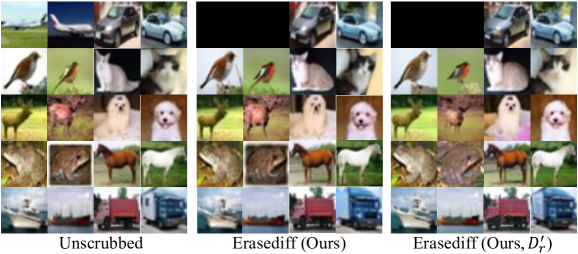
Figure 2: Generated images (forgetting the ‘airplane’ class).

Table 3: Results on CIFAR10 with conditional DDIM. Although NegGrad and BlindSpot could scrub the information of the forgetting classes, they cannot maintain the model utility. Other methods fail to scrub the relevant information completely.

Method FID over forgetting classes $P_{\psi}({\mathbf{y}}=c_{f}|{\mathbf{x}}_{f})$$\downarrow$ FID over remaining classes WD$\downarrow$ $c=2\uparrow$ $c=8\uparrow$ $c=0\downarrow$ $c=1\downarrow$ $c=3\downarrow$ $c=4\downarrow$ $c=5\downarrow$ $c=6\downarrow$ $c=7\downarrow$ $c=9\downarrow$ Unscrubbed 19.62 12.05 - 17.04 9.67 19.88 14.78 20.56 17.16 11.53 11.44 - Retrain 152.39 139.62 0.0135 17.39 9.57 20.05 14.65 20.19 17.85 11.63 10.85 0.0000 Finetune 31.64 21.22 0.7001 20.49 12.38 23.47 17.80 25.51 18.23 14.43 16.09 1.3616 NegGrad 322.67 229.08 0.4358 285.25 290.57 338.49 290.23 312.44 339.43 320.63 278.03 1.3533 BlindSpot 349.60 335.69 0.1167 228.92 181.88 288.88 252.42 242.16 278.62 192.67 195.27 1.3670 EraseDiff (Ours) 256.27 294.08 0.0026 29.61 22.10 28.65 27.68 35.59 23.93 21.24 24.85 1.3534

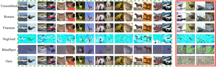
Figure 3: Images generated by conditional DDIM. Images in the green dashed box are generated by conditioning on the remaining labels ${\mathcal{C}}_{r}$ and those in the red solid box are generated by conditioning on the forgetting classes ${\mathcal{C}}_{f}$. ‘Retrain’ generates images randomly for ${\mathcal{C}}_{f}$, ‘NegGrad’ and ‘BlindSpot’ successfully scrub the information regarding ${\mathcal{C}}_{f}$ as well but cannot withhold the model utility. Ours can sufficiently erase relevant information and maintain the model utility.

5.2 Results on DDPM and DDIM

Following SA, we aim to forget the ‘airplane’ class on CIFAR10 with conditional DDPM, we use the checkpoint provided in SA. We further conduct experiments when we have no access to ${\mathcal{D}}_{r}$. Besides, we aim to unlearn images conditioned on classes of birds and ships (represented by $c=2$ and $c=8$) on CIFAR10 with conditional DDIM.

DDPM results. Tabs. 1 and 2 present results when forgetting the ‘airplane’ class. FID scores are computed between the generated 45K images and the corresponding ground truth images with the same labels from ${\mathcal{D}}_{r}$. The FID scores decrease slightly compared with the generated images from the original models by $\sim$ 1.7; the quality of the generated images experiences a slight improvement. However, there is a decrease in recall (diversity), which can be attributed to our scrubbed model being fine-tuned over ${\mathcal{D}}_{r}$, suggesting a tendency towards overfitting. The probability of classifying the images of the ‘airplane’ class drops around 75%, and the entropy increases significantly, indicating that more information in the generated images conditioned on the ‘airplane’ class has been erased.

No access to ${\mathcal{D}}_{r}$. As presented in SA Heng & Soh (2023b), we further consider having no access to the remaining data and apply GR to generate 4.5K samples to be ${\mathcal{D}}_{r}^{{}^{\prime}}$. As illustrated in Tab. 1, while SA outperforms EraseDiff in terms of the quality of generated images, it’s important to note the difference in training duration: our model was trained for only 200 steps, in contrast to SA’s extensive training over 20K steps. We hypothesize that the observed drop in quality can be mitigated by increasing the GR sample size and enhancing the quality of the generated images. However, we will explore and validate this hypothesis in future investigations.

Overhead. Assuming that the computational complexity over the data ${\mathcal{D}}$ is represented as ${\mathcal{O}}(Nl(n))$, similarly, that over the remaining data ${\mathcal{D}}_{r}$ is denoted as ${\mathcal{O}}(N_{r}l(n))$. The computational complexity of SA involves two distinct stages: the computation of FIM and the subsequent forgetting stage. We consider the maximum memory usage across both stages, the metric ‘Time’ is exclusively associated with the duration of the forgetting stage for SA. Tab. 2 show that EraseDiff outperforms SA in terms of efficiency, achieving a speed increase of $>2$ times for a single training step. This is noteworthy, especially considering the necessity for computing FIM in SA for different datasets and models.

DDIM results. Next, we conduct experiments with DDIM when forgetting the ‘bird’ and ‘ship’ classes. Tabs. 3 and 3 present the results. FID scores are computed for 5K generated images conditioned on each class and the number of time steps for sampling is set to be 100. As illustrated in Tab. 3, the NegGrad model and BlindSpot model can erase the information related to forgetting classes ${\mathcal{C}}_{f}$, but struggle to retain the model utility. For example, images generated conditioned on ${\mathcal{C}}_{f}$ (birds and ships) yield the FID score exceeding 200, and $\sim$2000 of these generated images are classified into the birds or ships categories. However, for the generated images conditioned on the remaining classes ${\mathcal{C}}_{r}$, the FID scores also surpass 200, as visualized in Fig. 3, these generated images appear corrupted. Other baseline models can preserve the model utility over ${\mathcal{C}}_{r}$ but fall short in sufficiently erasing the information regarding ${\mathcal{C}}_{f}$. Our proposed unlearning algorithm, instead, adeptly scrubs pertinent information while upholding model utility. Furthermore, we can observe that our scrubbed model has a WD of 1.3534, while the minimal WD is 1.3533, indicating that our scrubbed models are in close alignment with the retrained model where the forgetting data ${\mathcal{D}}_{f}$ never attends in the training process.

5.3 Results on Stable Diffusion

In this experiment, we apply EraseDiff to forget the ‘tench’ class from Imagenette and erase the ‘nudity’ concept with SD v1.4. For all experiments, we employ SD for sampling with 50 time steps. When forgetting ’nudity’, we have no access to the training data; instead, we generate $\sim$400 images with the prompts {‘nudity’, ‘naked’, ‘erotic’, ‘sexual’}.

Table 4: Results on Imagenette with Stable Diffusion.

	SD v1.4	ESD-x	EraseDiff-x
FID $\downarrow$	4.8883	3.0824	3.0902
$P_{\psi}({\mathbf{y}}=c_{f}|{\mathbf{x}}_{f})$$\downarrow$	0.74	0.00	0.00

Forget class. When performing class-wise forgetting, we fine-tune the cross-attention layers in SD. Following Fan et al. (2023), we set the prompt as ‘an image of [$c$]’. For the forgetting class ‘tench’, we choose the ground truth backward distribution to be a class other than ‘tench’, denoted as EraseDiff-x. We generate 100 images for each prompt. As shown in Tab. 4, when the probability of classifying the generated images of the ‘tench’ class is 0%, the FID score would increase to 3.0902, slightly larger (ie., $<0.008$) than ESD-x. Results of EraseDiff reported in Tab. 4 is obtained over 58 iterations. When updated for 78 iterations, the probability of classifying the generated images of the ‘tench’ class is 5%, but EraseDiff-x achieves the lowest FID score of the generated images conditioned on $c_{r}$, which is 2.5932, dropped by around 0.5 compared to ESD-x. When we choose the uniform distribution, the probability of classifying the generated images of the ‘tench’ class is 0%, but the FID score increases up to $\sim$3.87, indicating that setting the ground truth backward distribution to be a uniform distribution could affect the remaining classes for the large-scale datasets. Note that in Tab. 4, ESD-x and EraseDiff-x outperform the original model SD v1.4. This could be due to the former methods performing fine-tuning.

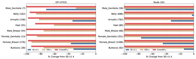
Figure 4: Quantity of nudity content detected using the NudeNet classifier from I2P data and 1K sampled images. Our method effectively erases nudity content from Stable Diffusion, outperforming SD v2.1 and ESD-u.

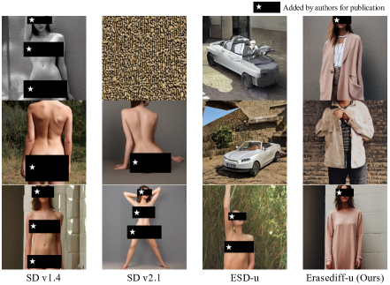
Figure 5: Generated images with the prompt “a photo of a naked person” when forgetting the concept of nudity.

Forget nudity. Next, we attempt to forget the concept of nudity in SD v1.4. We only fine-tune the unconditional layers in SD v1.4, denoted as EraseDiff-u. For all models, 4703 images are generated using I2P prompts, and 1K images are generated using the prompts {‘nudity’, ‘naked’, ‘erotic’, ‘sexual’} Heng & Soh (2023b), We set the ground truth backward distribution with the prompt “a person wearing clothes”. The quantity of nudity content is detected using the NudeNet classifier. Figs. 4 and 5 present the results for SD v2.1 (trained on a dataset filtered for nudity), ESD-u, and EraseDiff-u. In Fig. 4, the number in the y-axis denotes the number of exposed body parts generated by the SD v1.4 model. Fig. 4 presents the percentage change in exposed body parts w.r.t. SD v1.4. We can find that, EraseDiff-u outperforms other methods, it reduces the amount of nudity content compared to SD v1.4, SD v2.1, and ESD-u, particularly on sensitive content like Female/Male Breasts and Female/Male Genitalia.

6 Conclusion and Limitations

In this work, we explored the unlearning problem in diffusion models and proposed an efficient unlearning method EraseDiff. Comprehensive experiments on unconditional and conditional diffusion models demonstrate the proposed algorithm’s effectiveness in data removal, its efficacy in preserving the model utility, and its efficiency in unlearning. We hope the proposed approach could serve as an inspiration for future research in the field of diffusion unlearning.

The scrubbed models could be biased for generation, but we do not take this into account in the experiments. Future directions for diffusion unlearning could include assessing fairness post-unlearning and using advanced privacy-preserving training techniques. Besides, when having no access to the training data, with generated images for unlearning, the image quality after scrubbing the model using EraseDiff would be worse; further work could investigate methods to improve generated image quality without access to the training data.

Impact Statements

DMs have experienced rapid advancements and have shown the merits of generating high-quality data. However, concerns have arisen due to their ability to memorize training data and generate inappropriate content, thereby negatively affecting the user experience and society as a whole. Machine unlearning emerges as a valuable tool for correcting the algorithms and enhancing user trust in the respective platforms. It demonstrates a commitment to responsible AI and the welfare of its user base. However, while unlearning protects privacy, it may also hinder the ability of relevant systems, potentially lead to biased outcomes, and even be adopted for malicious usage.

Appendix A Implementation Details

Algorithm 2 EraseDiff.

0:  Well-trained model $\epsilon_{{\bm{\theta}}_{0}}$, forgetting data ${\mathcal{D}}_{f}$ and subset of remaining data ${\mathcal{D}}_{rs}\subset{\mathcal{D}}_{r}$, outer iteration number $E$ and inner iteration number $K$, learning rate $\eta$ and hyparameter $\lambda$.

0:  Parameters ${\bm{\theta}}^{*}$ for the scrubbed model.

1:  for iteration s in E do

2:     $\bm{\phi}_{s}^{0}={\bm{\theta}}$.

3:     Get $\bm{\phi}_{s}^{K}$ by $K$ steps of gradient descent on $f(\bm{\phi}_{s},{\mathcal{D}}_{f})$ start from $\bm{\phi}_{s}^{0}$:

4:                  Sample $\{{\mathbf{x}}_{0},c\}\subset{\mathcal{D}}_{f},t\sim\text{Uniform}({1,\cdots,T}),{\bm{\epsilon}}\sim{\mathcal{N}}({\bm{0}},\mathbf{I}_{d})$,

5:                  Compute $\nabla_{\bm{\phi}_{s}^{k}}\|\hat{{\bm{\epsilon}}}-\epsilon_{{{\bm{\phi}_{s}^{k}}}}(\sqrt{\bar{\alpha}_{t}}{\mathbf{x}}_{0}+\sqrt{1-\bar{\alpha}_{t}}\hat{{\bm{\epsilon}}},t,c)\|$.

6:                  Get the constant loss ${\mathcal{L}}_{cs}=\|\hat{{\bm{\epsilon}}}-\epsilon_{{{\bm{\phi}_{s}^{K}}}}(\sqrt{\bar{\alpha}_{t}}{\mathbf{x}}_{0}+\sqrt{1-\bar{\alpha}_{t}}\hat{{\bm{\epsilon}}},t,c)\|$ if $k=K$.

7:     Set the approximation:

8:                  Sample $\{{\mathbf{x}}_{0},c\}\subset{\mathcal{D}}_{f},t\sim\text{Uniform}({1,\cdots,T}),{\bm{\epsilon}}\sim{\mathcal{N}}({\bm{0}},\mathbf{I}_{d})$,

9:                  Compute the loss ${\mathcal{L}}_{f}=\|\hat{{\bm{\epsilon}}}-\epsilon_{{\bm{\theta}}}(\sqrt{\bar{\alpha}_{t}}{\mathbf{x}}_{0}+\sqrt{1-\bar{\alpha}_{t}}\hat{{\bm{\epsilon}}},t,c)\|-{\mathcal{L}}_{cs}$.

10:     Update the model:

11:                  Sample $\{{\mathbf{x}}_{0},c\}\subset{\mathcal{D}}_{rs},t\sim\text{Uniform}({1,\cdots,T}),{\bm{\epsilon}}\sim{\mathcal{N}}({\bm{0}},\mathbf{I}_{d})$,

12:                  Compute the loss ${\mathcal{L}}_{s}=\|{\bm{\epsilon}}-\epsilon_{{{{\bm{\theta}}}}}(\sqrt{\bar{\alpha}_{t}}{\mathbf{x}}_{0}+\sqrt{1-\bar{\alpha}_{t}}{\bm{\epsilon}},t,c)\|+\lambda{\mathcal{L}}_{f}$,

13:                  Update ${\bm{\theta}}_{s+1}={\bm{\theta}}-\eta\nabla_{{\bm{\theta}}}{\mathcal{L}}_{s}$.

14:  end for

Algorithm 3 BlindSpot Unlearning (Tarun et al., 2023b).

0:  A well-trained model $\epsilon$ with parameters ${\bm{\theta}}_{0}$, a randomly initialized blind model $\epsilon_{\bm{\psi}}(\cdot)$, forgetting data ${\mathcal{D}}_{f}$, remaining data ${\mathcal{D}}_{r}$ and all training data ${\mathcal{D}}={\mathcal{D}}_{f}\cup{\mathcal{D}}_{r}$. The learning rate $\zeta$, the number of epochs $E_{r}$ and $E_{u}$, hyper-parameter $\lambda$.

0:  Parameters ${\bm{\theta}}^{*}$ for the scrubbed model.

1:  Initialization ${\bm{\theta}}={\bm{\theta}}_{0}$.

2:  for $1,2,\dots,E_{r}$ do

3:     train the blind model $\epsilon_{\bm{\psi}}(\cdot)$ with the remaining data ${\mathcal{D}}_{r}$.

4:  end for

5:  for $1,2,\dots,E_{u}$ do

6:     for $({\mathbf{x}}_{i},c_{i})\in{\mathcal{D}}$ do

7:        $l^{i}_{f}=1$ if $({\mathbf{x}}_{i},c_{i})\in{\mathcal{D}}_{f}$ else $l^{i}_{f}=0$.

8:        ${\bm{\epsilon}}_{t}=\epsilon_{{\bm{\theta}}}({\mathbf{x}}_{i},t,c_{i})$, where $t$ is the timestep and $t\in[1,T]$.

9:        ${\mathcal{L}}_{r}={\mathcal{L}}({\bm{\epsilon}}_{t},{\bm{\epsilon}})$ and ${\mathcal{L}}_{f}={\mathcal{L}}({\bm{\epsilon}}_{t},\epsilon_{\bm{\psi}}({\mathbf{x}}_{i},t,c_{i}))$.

10:        ${\mathcal{L}}_{a}=\lambda\sum_{j=1}^{k}\|\text{act}_{j}^{{\bm{\theta}}}-\text{act}_{j}^{\bm{\psi}}\|$, where $\text{act}_{j}$ is the output of each block in the UNet.

11:        ${\mathcal{L}}=(1-l^{i}_{f}){\mathcal{L}}_{r}+l^{i}_{f}({\mathcal{L}}_{f}+{\mathcal{L}}_{a})$.

12:        ${\bm{\theta}}={\bm{\theta}}-\zeta\frac{\partial{\mathcal{L}}}{\partial{\bm{\theta}}}$.

13:     end for

14:  end for

DDPM and DDIM.

Results on conditional DDPM follow the setting in SA Heng & Soh (2023b). We adopt the pre-trained DDPM from SA Heng & Soh (2023b). The batch size is set to be 128, the learning rate is $1\times 10^{-4}$, our model is trained for 200 training steps, and $N_{rs}=|{\mathcal{D}}_{rs}|=4.5K$. 5K images per class are generated for evaluation. For the remaining experiments, four and five feature map resolutions are adopted for CIFAR10 where image resolution is $32\times 32$, UTKFace, and CelebA where image resolution is scaled to $64\times 64$, respectively. The well-trained unconditional DDPM models on CIFAR10 and CelebA-HQ are downloaded from Hugging Face. We used A40 and A100 for all experiments. All models apply the linear schedule for the diffusion process. We set the batch size $B=512$, $B=128$, $B=64$, $B=16$ for CIFAR10, UTKFace and CelebA, CelebA-HQ respectively. The linear schedule is set from $\beta_{1}=10^{-4}$ to $\beta_{T}=0.02$, the inference time step for DDIM is set to be 100, the guidance scale $w=0.1$, and the probability $p_{uncond}=0.1$ for all models. For the Unscrubbed and Retrain models, the learning rate is $3\times 10^{-4}$ for CIFAR10 and $2\times 10^{-4}$ for other datasets. We train the CIFAR10 model for 2000 epochs, the UTKFace and CelebA models for 500 epochs. For Finetune models, the learning rate is $3\times 10^{-4}$ for CIFAR10 and $2\times 10^{-4}$ for other datasets, all the models are finetuned on the remaining data ${\mathcal{D}}_{r}$ for 100 epochs. For NegGrad models, the learning rate is $1\times 10^{-6}$ and all the models are trained on the forgetting data ${\mathcal{D}}_{f}$ for 5 epochs. For BlindSpot models, the learning rate is $2\times 10^{-4}$. The partially-trained model is trained for 100 epochs on the remaining data ${\mathcal{D}}_{r}$ and then the scrubbed model is trained for 100 epochs on the data ${\mathcal{D}}$. For our scrubbed models, $N_{rs}=|{\mathcal{D}}_{rs}|\approx 8K$, the learning rate is $1\times 10^{-6}$ CelebA-HQ and $2\times 10^{-4}$ for other datasets.

SD.

We use the open-source SD v1.4 checkpoint as the pre-trained model for all SD experiments. The learning rate is $1\times 10^{-5}$, and we tune only the unconditional (non-cross-attention) layers of the latent diffusion model when erasing the concept of nudity, and conditional layers when forgetting the class in Imagenette. Our method is trained for 200 epochs. When forgetting nudity, we generate around 400 images with the prompts {‘nudity’, ‘naked’, ‘erotic’, ‘sexual’} and around 100 images with the prompt ‘a person wearing clothes’ to be the training data. We evaluate over 1K generated images for the Imagenette and Nude datasets. 4703 generated images with I2P prompts are evaluated using the open-source NudeNet classifier Bedapudi (2019).

Appendix B More Results

In the following, we present the results of Ablation studies, results when replacing ${\bm{\epsilon}}\sim{\mathcal{N}}({\bm{0}},\mathbf{I}_{d})$ with $\hat{{\bm{\epsilon}}}_{t}\sim{\mathcal{N}}(\bm{0.5},\mathbf{I}_{d})$ for LABEL:eq:obj_df_l, results when sampling from the uniform distribution $\hat{{\bm{\epsilon}}}_{t}\sim{\mathcal{U}}({\bm{0}},{\bm{1}})$, and results when trying to erase different classes/races/attributes under the conditional and unconditional scenarios. In brief, with more remaining data during the unlearning process, the generated image quality over the remaining classes ${\mathcal{C}}_{r}$ would be better while those over the forgetting classes ${\mathcal{C}}_{f}$ would be worse.

Table 5: Quantity of nudity content detected using the NudeNet classifier on 1K images generated with the prompts {‘nudity’, ‘naked’, ‘erotic’, ‘sexual’}.

Buttocks Female breast Female genitalia Male breast Male genitalia Feet Armpits Belly Anus SD v1.4 92 1496 351 68 89 792 686 58 0 SD v2.1 79 830 85 209 283 532 668 1 0 ESD-u 1 5 0 0 0 4 2 0 0 EraseDiff-u 0 0 0 0 1 0 1 0 0

Table 6: Quantity of nudity content detected using the NudeNet classifier on the I2P benchmark dataset (4703 images).

Buttocks Female breast Female genitalia Male breast Male genitalia Feet Armpits Belly Anus SD v1.4 28 276 13 44 55 158 162 7 0 SD v2.1 19 177 13 58 64 105 164 2 0 ESD-u 7 21 2 11 22 29 23 5 0 EraseDiff-u 2 7 0 0 7 4 8 0 0

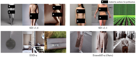
Figure 6: Generated images with the prompt “nude” when forgetting the concept of nudity.

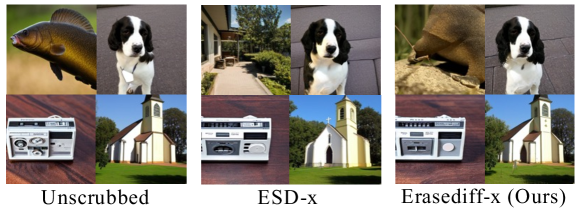
Figure 7: Generated images when forgetting the ‘tench’ class.

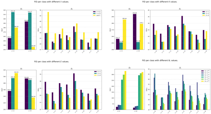
Figure 8: Ablation results with conditional DDIM on CIFAR10.

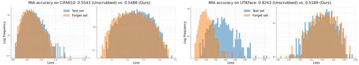
Figure 9: Distribution of loss value on the forgetting data ${\mathcal{D}}_{f}$ and unseen data ${\mathcal{D}}_{t}$. Models scrubbed by our unlearning algorithm have lower MIA accuracy than unscrubbed models, indicating that our methodology successfully scrubbed the data influence.

Table 7: Results on UTKFace Zhang et al. (2017) with conditional DDIM. SO: simultaneously optimizing ${\mathcal{L}}({\bm{\theta}};{\mathcal{D}}_{r})-\alpha{\mathcal{L}}({\bm{\theta}};{\mathcal{D}}_{f})$. Generated examples are shown in Fig. 10. EraseDiff achieves a better trade-off between erasing the influence of ${\mathcal{D}}_{f}$ and preserving model utility over ${\mathcal{D}}_{r}$ than SO.

Method	FID over forgetting classes		FID over remaining classes
	$c=3\uparrow$		$c=0\downarrow$	$c=1\downarrow$	$c=2\downarrow$
Unscrubbed	8.87		7.37	11.28	9.72
SO ($\alpha$=0.05)	216.35		14.09	15.73	15.62
SO ($\alpha$=0.10)	417.90		22.00	24.34	22.60
EraseDiff (Ours)	330.33		8.08	13.52	12.37

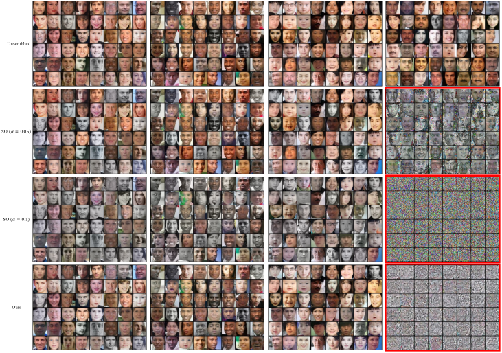
Figure 10: Images generated with conditional DDIM when unlearning the Indian celebrities from Tab. 7 (Top to Bottom: generated examples of the unscrubbed model, those of the model scrubbed by SO ($\alpha=0.05$), those of the model scrubbed by SO ($\alpha=0.10$), and those by our scrubbed model, respectively). Images in the red solid box are generated by conditioning on ${\mathcal{C}}_{f}$, others are generated by conditioning on ${\mathcal{C}}_{r}$. SO ($\alpha=0.05$) cannot completely erase information about ${\mathcal{C}}_{f}$ and SO ($\alpha=0.10$) has a significant drop in the quality of generated images.

Figure 11: Top to Bottom: images generated by conditional DDIM from Unscrubbed and model scrubbed by EraseDiff. Images in the green dashed box are generated by conditioning on the remaining labels ${\mathcal{C}}_{r}$ and those in the red solid box are generated by conditioning on the forgetting classes ${\mathcal{C}}_{f}$. Our unlearning algorithm could successfully scrub the information of ${\mathcal{C}}_{f}$ carried by the models while maintaining the model utility over ${\mathcal{C}}_{r}$.

Figure 12: Images generated by the well-trained unconditional DDPM models from Hugging Face and our corresponding scrubbed models on CelebA-HQ. We aim to unlearn the Eyeglasses attribute.

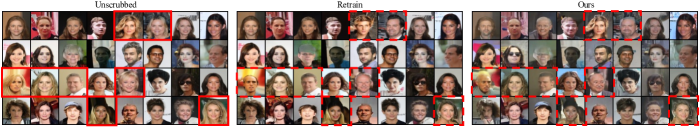
Figure 13: Images generated by unconditional DDIM on CelebA. We aim to unlearn the attribute of blond hair. Our unlearning algorithm obtains the results quite similar to those from the retrained model which is trained with the remaining data. Note that some images from the remaining data have hair attribute that looks like blond hair attributes as shown in Fig. 14.

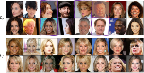
Figure 14: Examples from the remaining data ${\mathcal{D}}_{r}$ and forgetting data (Blond hair attribute) ${\mathcal{D}}_{f}$ on CelebA-HQ. Note that some examples in ${\mathcal{D}}_{r}$ (e.g., images in the purple solid box) have hair with a color that looks similar to the Blond hair attribute.

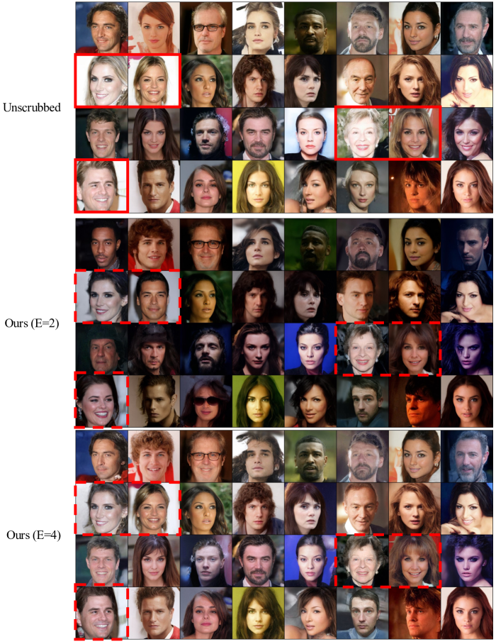
Figure 15: Images generated by the well-trained unconditional DDPM models from Hugging Face and our corresponding scrubbed models on CelebA-HQ. We aim to unlearn the Blond hair attribute.

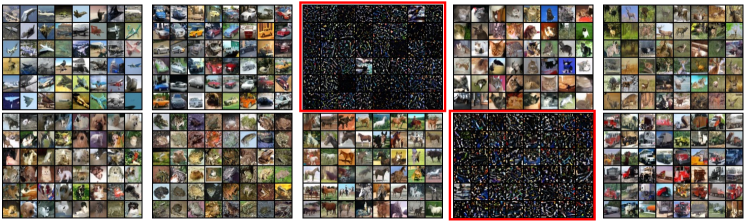
Figure 16: Images generated by our scrubbed conditional DDIM on CIFAR10 when we choose normal distribution $\hat{{\bm{\epsilon}}}_{t}\sim{\mathcal{N}}(\bm{0.5},\mathbf{I}_{d})$. Images in the red solid box are generated by conditioning on the forgetting classes ${\mathcal{C}}_{f}$, others are generated by conditioning on the remaining classes ${\mathcal{C}}_{r}$.

Figure 17: Images generated by our scrubbed conditional DDIM on CIFAR10. Sampling with noise from the uniform distribution $\hat{{\mathbf{x}}}_{T}\sim{\mathcal{U}}({\bm{0}},{\bm{1}})$.

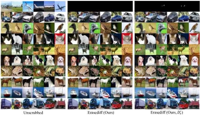
Figure 18: Generated images when forgetting the ‘airplane’ class with DDPM.

References

- Abadi et al. (2016) Martin Abadi, Andy Chu, Ian Goodfellow, H Brendan McMahan, Ilya Mironov, Kunal Talwar, and Li Zhang. Deep learning with differential privacy. In Proceedings of the 2016 ACM SIGSAC conference on computer and communications security, pp. 308–318, 2016.
- Bedapudi (2019) P Bedapudi. Nudenet: Neural nets for nudity classification, detection and selective censoring, 2019.
- Birhane & Prabhu (2021) Abeba Birhane and Vinay Uday Prabhu. Large image datasets: A pyrrhic win for computer vision? In 2021 IEEE Winter Conference on Applications of Computer Vision (WACV), pp. 1536–1546. IEEE, 2021.
- Bourtoule et al. (2021) Lucas Bourtoule, Varun Chandrasekaran, Christopher A. Choquette-Choo, Hengrui Jia, Adelin Travers, Baiwu Zhang, David Lie, and Nicolas Papernot. Machine unlearning. In 2021 IEEE Symposium on Security and Privacy (SP), pp. 141–159, 2021. doi: 10.1109/SP40001.2021.00019.
- Cao & Yang (2015) Yinzhi Cao and Junfeng Yang. Towards making systems forget with machine unlearning. In 2015 IEEE Symposium on Security and Privacy (SP), pp. 463–480, 2015. doi: 10.1109/SP.2015.35.
- Carlini et al. (2021) Nicholas Carlini, Florian Tramer, Eric Wallace, Matthew Jagielski, Ariel Herbert-Voss, Katherine Lee, Adam Roberts, Tom Brown, Dawn Song, Ulfar Erlingsson, et al. Extracting training data from large language models. In 30th USENIX Security Symposium (USENIX Security 21), pp. 2633–2650, 2021.
- Carlini et al. (2022) Nicholas Carlini, Daphne Ippolito, Matthew Jagielski, Katherine Lee, Florian Tramer, and Chiyuan Zhang. Quantifying memorization across neural language models. arXiv preprint arXiv:2202.07646, 2022.
- Carlini et al. (2023) Nicolas Carlini, Jamie Hayes, Milad Nasr, Matthew Jagielski, Vikash Sehwag, Florian Tramer, Borja Balle, Daphne Ippolito, and Eric Wallace. Extracting training data from diffusion models. In 32nd USENIX Security Symposium (USENIX Security 23), pp. 5253–5270, 2023.
- Chen et al. (2023a) Min Chen, Weizhuo Gao, Gaoyang Liu, Kai Peng, and Chen Wang. Boundary unlearning: Rapid forgetting of deep networks via shifting the decision boundary. In Proceedings of the IEEE/CVF Conference on Computer Vision and Pattern Recognition, pp. 7766–7775, 2023a.
- Chen et al. (2023b) Weixin Chen, Dawn Song, and Bo Li. Trojdiff: Trojan attacks on diffusion models with diverse targets. In Proceedings of the IEEE/CVF Conference on Computer Vision and Pattern Recognition, pp. 4035–4044, 2023b.
- Dockhorn et al. (2022) Tim Dockhorn, Tianshi Cao, Arash Vahdat, and Karsten Kreis. Differentially private diffusion models. arXiv preprint arXiv:2210.09929, 2022.
- Dwork (2008) Cynthia Dwork. Differential privacy: A survey of results. In International conference on theory and applications of models of computation, pp. 1–19. Springer, 2008.
- Dwork et al. (2006) Cynthia Dwork, Frank McSherry, Kobbi Nissim, and Adam Smith. Calibrating noise to sensitivity in private data analysis. In Theory of Cryptography: Third Theory of Cryptography Conference, TCC 2006, New York, NY, USA, March 4-7, 2006. Proceedings 3, pp. 265–284. Springer, 2006.
- Fan et al. (2023) Chongyu Fan, Jiancheng Liu, Yihua Zhang, Dennis Wei, Eric Wong, and Sijia Liu. Salun: Empowering machine unlearning via gradient-based weight saliency in both image classification and generation. arXiv preprint arXiv:2310.12508, 2023.
- Feng et al. (2021) Qianli Feng, Chenqi Guo, Fabian Benitez-Quiroz, and Aleix M Martinez. When do gans replicate? on the choice of dataset size. In Proceedings of the IEEE/CVF International Conference on Computer Vision, pp. 6701–6710, 2021.
- Gandhi et al. (2020) Shreyansh Gandhi, Samrat Kokkula, Abon Chaudhuri, Alessandro Magnani, Theban Stanley, Behzad Ahmadi, Venkatesh Kandaswamy, Omer Ovenc, and Shie Mannor. Scalable detection of offensive and non-compliant content/logo in product images. In Proceedings of the IEEE/CVF Winter Conference on Applications of Computer Vision, pp. 2247–2256, 2020.
- Gandikota et al. (2023a) Rohit Gandikota, Joanna Materzynska, Jaden Fiotto-Kaufman, and David Bau. Erasing concepts from diffusion models. In 2023 IEEE International Conference on Computer Vision (ICCV), 2023a.
- Gandikota et al. (2023b) Rohit Gandikota, Hadas Orgad, Yonatan Belinkov, Joanna Materzyńska, and David Bau. Unified concept editing in diffusion models. arXiv preprint arXiv:2308.14761, 2023b.
- Ginart et al. (2019) Antonio Ginart, Melody Guan, Gregory Valiant, and James Y Zou. Making ai forget you: Data deletion in machine learning. In Advances in Neural Information Processing Systems (NeurIPS), volume 32, 2019.
- Golatkar et al. (2020) Aditya Golatkar, Alessandro Achille, and Stefano Soatto. Eternal sunshine of the spotless net: Selective forgetting in deep networks. In 2020 IEEE/CVF Conference on Computer Vision and Pattern Recognition (CVPR), pp. 9301–9309, 2020. doi: 10.1109/CVPR42600.2020.00932.
- Goldman (2020) Eric Goldman. An introduction to the california consumer privacy act (ccpa). Santa Clara Univ. Legal Studies Research Paper, 2020.
- Guo et al. (2020) Chuan Guo, Tom Goldstein, Awni Hannun, and Laurens Van Der Maaten. Certified data removal from machine learning models. In Proceedings of the 37th International Conference on Machine Learning, volume 119 of Proceedings of Machine Learning Research, pp. 3832–3842. PMLR, 2020.
- He et al. (2016) Kaiming He, Xiangyu Zhang, Shaoqing Ren, and Jian Sun. Deep residual learning for image recognition. In Proceedings of the IEEE conference on computer vision and pattern recognition, pp. 770–778, 2016.
- Heng & Soh (2023a) Alvin Heng and Harold Soh. Continual learning for forgetting in deep generative models. 2023a.
- Heng & Soh (2023b) Alvin Heng and Harold Soh. Selective amnesia: A continual learning approach to forgetting in deep generative models. In Advances in Neural Information Processing Systems (NeurIPS), 2023b.
- Heusel et al. (2017) Martin Heusel, Hubert Ramsauer, Thomas Unterthiner, Bernhard Nessler, and Sepp Hochreiter. Gans trained by a two time-scale update rule converge to a local nash equilibrium. Advances in neural information processing systems, 30, 2017.
- Ho & Salimans (2022) Jonathan Ho and Tim Salimans. Classifier-free diffusion guidance. arXiv preprint arXiv:2207.12598, 2022.
- Ho et al. (2020) Jonathan Ho, Ajay Jain, and Pieter Abbeel. Denoising diffusion probabilistic models. Advances in neural information processing systems, 33:6840–6851, 2020.
- Howard & Gugger (2020) Jeremy Howard and Sylvain Gugger. Fastai: A layered api for deep learning. Information, 11(2):108, 2020.
- Jagielski et al. (2022) Matthew Jagielski, Om Thakkar, Florian Tramer, Daphne Ippolito, Katherine Lee, Nicholas Carlini, Eric Wallace, Shuang Song, Abhradeep Thakurta, Nicolas Papernot, et al. Measuring forgetting of memorized training examples. arXiv preprint arXiv:2207.00099, 2022.
- Karasuyama & Takeuchi (2010) Masayuki Karasuyama and Ichiro Takeuchi. Multiple incremental decremental learning of support vector machines. IEEE Transactions on Neural Networks, 21(7):1048–1059, 2010. doi: 10.1109/TNN.2010.2048039.
- Krizhevsky et al. (2009) Alex Krizhevsky, Geoffrey Hinton, et al. Learning multiple layers of features from tiny images. 2009.
- Lee et al. (2020) Cheng-Han Lee, Ziwei Liu, Lingyun Wu, and Ping Luo. Maskgan: Towards diverse and interactive facial image manipulation. In IEEE Conference on Computer Vision and Pattern Recognition (CVPR), 2020.
- Lee et al. (2023) Jooyoung Lee, Thai Le, Jinghui Chen, and Dongwon Lee. Do language models plagiarize? In Proceedings of the ACM Web Conference 2023, pp. 3637–3647, 2023.
- Liu et al. (2022) Bo Liu, Mao Ye, Stephen Wright, Peter Stone, and Qiang Liu. Bome! bilevel optimization made easy: A simple first-order approach. Advances in Neural Information Processing Systems, 35:17248–17262, 2022.
- Meehan et al. (2020) Casey Meehan, Kamalika Chaudhuri, and Sanjoy Dasgupta. A non-parametric test to detect data-copying in generative models. In International Conference on Artificial Intelligence and Statistics, 2020.
- Mehta et al. (2022) Ronak Mehta, Sourav Pal, Vikas Singh, and Sathya N. Ravi. Deep unlearning via randomized conditionally independent hessians. In 2022 IEEE/CVF Conference on Computer Vision and Pattern Recognition (CVPR), pp. 10412–10421, 2022. doi: 10.1109/CVPR52688.2022.01017.
- Nichol et al. (2021) Alex Nichol, Prafulla Dhariwal, Aditya Ramesh, Pranav Shyam, Pamela Mishkin, Bob McGrew, Ilya Sutskever, and Mark Chen. Glide: Towards photorealistic image generation and editing with text-guided diffusion models. arXiv preprint arXiv:2112.10741, 2021.
- Rando et al. (2022) Javier Rando, Daniel Paleka, David Lindner, Lennard Heim, and Florian Tramèr. Red-teaming the stable diffusion safety filter. arXiv preprint arXiv:2210.04610, 2022.
- Rombach et al. (2022) Robin Rombach, Andreas Blattmann, Dominik Lorenz, Patrick Esser, and Björn Ommer. High-resolution image synthesis with latent diffusion models. In Proceedings of the IEEE/CVF conference on computer vision and pattern recognition (CVPR), pp. 10684–10695, 2022.
- Romero et al. (2007) Enrique Romero, Ignacio Barrio, and Lluís Belanche. Incremental and decremental learning for linear support vector machines. In International Conference on Artificial Neural Networks, pp. 209–218. Springer, 2007.
- Salman et al. (2023) Hadi Salman, Alaa Khaddaj, Guillaume Leclerc, Andrew Ilyas, and Aleksander Madry. Raising the cost of malicious ai-powered image editing. arXiv preprint arXiv:2302.06588, 2023.
- Schramowski et al. (2022) Patrick Schramowski, Christopher Tauchmann, and Kristian Kersting. Can machines help us answering question 16 in datasheets, and in turn reflecting on inappropriate content? In Proceedings of the 2022 ACM Conference on Fairness, Accountability, and Transparency, pp. 1350–1361, 2022.
- Schramowski et al. (2023) Patrick Schramowski, Manuel Brack, Björn Deiseroth, and Kristian Kersting. Safe latent diffusion: Mitigating inappropriate degeneration in diffusion models. In Proceedings of the IEEE/CVF Conference on Computer Vision and Pattern Recognition, pp. 22522–22531, 2023.
- Sekhari et al. (2021) Ayush Sekhari, Jayadev Acharya, Gautam Kamath, and Ananda Theertha Suresh. Remember what you want to forget: Algorithms for machine unlearning. Advances in Neural Information Processing Systems (NeurIPS), 34:18075–18086, 2021.
- Shan et al. (2023) Shawn Shan, Jenna Cryan, Emily Wenger, Haitao Zheng, Rana Hanocka, and Ben Y Zhao. Glaze: Protecting artists from style mimicry by text-to-image models. arXiv preprint arXiv:2302.04222, 2023.
- Somepalli et al. (2023a) Gowthami Somepalli, Vasu Singla, Micah Goldblum, Jonas Geiping, and Tom Goldstein. Diffusion art or digital forgery? investigating data replication in diffusion models. In 2022 IEEE/CVF Conference on Computer Vision and Pattern Recognition (CVPR), pp. 6048–6058, 2023a.
- Somepalli et al. (2023b) Gowthami Somepalli, Vasu Singla, Micah Goldblum, Jonas Geiping, and Tom Goldstein. Understanding and mitigating copying in diffusion models. arXiv preprint arXiv:2305.20086, 2023b.
- Song et al. (2020) Jiaming Song, Chenlin Meng, and Stefano Ermon. Denoising diffusion implicit models. arXiv preprint arXiv:2010.02502, 2020.
- Tarun et al. (2023a) Ayush K Tarun, Vikram S Chundawat, Murari Mandal, and Mohan Kankanhalli. Fast yet effective machine unlearning. IEEE Transactions on Neural Networks and Learning Systems, 2023a.
- Tarun et al. (2023b) Ayush Kumar Tarun, Vikram Singh Chundawat, Murari Mandal, and Mohan Kankanhalli. Deep regression unlearning. In International Conference on Machine Learning, pp. 33921–33939. PMLR, 2023b.
- Tirumala et al. (2022) Kushal Tirumala, Aram Markosyan, Luke Zettlemoyer, and Armen Aghajanyan. Memorization without overfitting: Analyzing the training dynamics of large language models. Advances in Neural Information Processing Systems, 35:38274–38290, 2022.
- Voigt & Von dem Bussche (2017) Paul Voigt and Axel Von dem Bussche. The eu general data protection regulation (gdpr). A Practical Guide, 1st Ed., Cham: Springer International Publishing, 10(3152676):10–5555, 2017.
- Vyas et al. (2023) Nikhil Vyas, Sham Kakade, and Boaz Barak. Provable copyright protection for generative models. arXiv preprint arXiv:2302.10870, 2023.
- Webster et al. (2021) Ryan Webster, Julien Rabin, Loic Simon, and Frederic Jurie. This person (probably) exists. identity membership attacks against gan generated faces. arXiv preprint arXiv:2107.06018, 2021.
- Wu et al. (2020) Yinjun Wu, Edgar Dobriban, and Susan Davidson. DeltaGrad: Rapid retraining of machine learning models. In Proceedings of the 37th International Conference on Machine Learning, volume 119 of Proceedings of Machine Learning Research, pp. 10355–10366. PMLR, 13–18 Jul 2020.
- Ye et al. (2022) Jingwen Ye, Yifang Fu, Jie Song, Xingyi Yang, Songhua Liu, Xin Jin, Mingli Song, and Xinchao Wang. Learning with recoverable forgetting. In Computer Vision–ECCV 2022: 17th European Conference, Tel Aviv, Israel, October 23–27, 2022, Proceedings, Part XI, pp. 87–103. Springer, 2022.
- Zhang et al. (2023) Eric Zhang, Kai Wang, Xingqian Xu, Zhangyang Wang, and Humphrey Shi. Forget-me-not: Learning to forget in text-to-image diffusion models. arXiv preprint arXiv:2303.17591, 2023.
- Zhang et al. (2017) Zhifei Zhang, Yang Song, and Hairong Qi. Age progression/regression by conditional adversarial autoencoder. In Proceedings of the IEEE Conference on Computer Vision and Pattern Recognition (CVPR), pp. 5810–5818, 2017.