Data-driven $h^{2}$ model reduction for linear discrete-time systems

Abstract

We present a new framework of $h^{2}$ optimal model reduction for linear discrete-time systems. Our main contribution is to create optimal reduced order models in the $h^{2}$-norm sense directly from the measurement data alone, without using the information of the original system. In particular, we focus on the fact that the gradient of the $h^{2}$ model reduction problem is expressed using the discrete-time Lyapunov equation and the discrete-time Sylvester equation, and derive the data-driven gradient. In the proposed algorithm, the initial point is chosen as the output of the existing data-driven methods. Numerical experiments are conducted to show that the proposed method produce better reduced order models in the $h^{2}$-norm sense than other data-driven model order reduction approaches.

I Introduction

With the development of computers, there are more and more situations in which large and complex systems are being handled. However, as the system size becomes larger, it may not be possible to analyze them in a practical amount of time. In such cases, model order reduction (MOR) methods are powerful tools, offering efficient ways to simplify complex systems. In systems control theory, MOR generates reduced order models (ROMs) that are capable of reproducing the input-output behavior of large-scale dynamical systems with high accuracy. The resulting ROMs have the advantage of being easier to manipulate and control, unlike the inherently larger systems. There are MOR methods based on Singular Value Decomposition (SVD) [1, 2, 3, 4, 5], Krylov subspaces (or moment matching methods) [6, 4, 7, 8], and the optimization of the $h^{2}$ (or $H^{2}$) norm [7, 9, 10, 11, 12]. These classical model reduction methods based on the state-space description of the system are known as model-based MOR. On the other hand, when a state-space description of the system is not available or computational modeling is difficult, it is desirable to create ROMs using the measurement data alone.

Data-driven model reduction constructs the ROMs that are capable of reproducing the input-output behavior of large-scale dynamical systems with high accuracy directly from the measurement data alone. Unlike traditional approaches, system identification is not required. Thus, there is no need to worry about errors introduced by system identification. Several well-known data-driven MOR methods have been proposed due to the increasing use of data. The data-driven balanced truncation method [13, 14, 15] is one of the common data-driven model reduction inspired by the balanced truncation method, which is a model-based MOR. In this method, balanced truncation is performed by using the measurement data. For example, [14] performs MOR by estimating the Gramians from the data information. Another well-known approach is Loewner framework [16, 17, 18, 19, 20]. In this approach, the Loewner and shifted Loewner matrices are first created from the frequency-response data, and then their SVD is performed. ROMs are created from the resulting projection. The time-domain data approach for Loewner framework is discussed in [21, 20]. Other data-driven methods, such as proper orthogonal decomposition (POD) [22] or dynamic mode decomposition (DMD) [23, 24] can also be employed. These approaches are the leading data-driven model reduction, but they may not yield optimal ROMs in the $h^{2}$-norm sense. In such cases, the output of the resulting reduced system may not approximate that of the original system.

In this paper, we propose a data-driven model reduction method for discrete-time linear systems. We focus on obtaining the optimal ROMs in the $h^{2}$-norm sense, using the measurement time-domain data. The contributions of this research are the following two points:

1) We propose a new framework for data-driven model reduction for discrete-time systems. We focus on obtaining the ROMs that perform well in terms of the $h^{2}$-norm, directly from the measurement data. In our approach, there is no need to use system identification methods, as in traditional approaches. Furthermore, under certain assumptions about the measurement data, we derive the gradients of the optimization problem characterized by the data.

2) We develop an algorithm for the proposed method and conduct numerical experiments. The proposed algorithm can be hybridized with existing data-driven MOR. Numerical experiments are conducted to show that the proposed method produces the ROMs that perform well in the $h^{2}$-norm sense compared with other data-driven MOR approaches.

The remainder of the paper is structured as follows. Section II describes the model-based $h^{2}$ MOR problem for the discrete-time systems. We describe the problem setting of this study in Section III. Section IV describes the data-driven $h^{2}$ MOR method proposed in this paper and its algorithm is explained in Section V. Section VI presents the results of numerical experiments for the initial points by the outputs of the existing data-driven methods. We conclude and discuss future work in Section VII.

Notation: We denote the imaginary unit by $\mathrm{i}$. We also denote the Frobenius norm, transpose, trace, the Moore-Penrose pseudoinverse, the $i$-th eigenvalue, and the $i$-th row vector of matrix $A$ by $\|A\|_{F}$, $A^{\top}$, $\operatorname{tr}A$, $A^{{\dagger}}$, $\lambda_{i}(A)$, and $A(i,:)$, respectively. In addition to that, we denote the complex conjugate transpose of $A\in\mathbb{C}^{n\times n}$ by $A^{*}\in\mathbb{C}^{n\times n}$. Furthermore, $(A,B)\in\mathbb{R}^{n\times n}\times\mathbb{R}^{n\times n}$ is called a regular matrix pencil if there exists $\lambda\in\mathbb{R}$ such that $A+\lambda B\in\mathbb{R}^{n\times n}$ is non-singular, and the spectra of $(A,B)$ is defined as the set of the solution $\lambda\in\mathbb{R}$ which satisfies the generalized eigenvalue problem $\det(A-\lambda B)$.

II Preliminaries

In this section, we summarize a model-based $h^{2}$ MOR [4, 7, 9, 10] for linear time-invariant (LTI) discrete-time dynamical systems

$$\begin{aligned} x_{k+1}&=Ax_{k}+Bu_{k},\\ y_{k}&=Cx_{k},\end{aligned}$$ (1)

with transfer function $H(z):=C(zI_{n}-A)^{-1}B$, where $k$ indicates the temporal iteration from a discrete dynamical system and the input, the state, and the output vectors at time $t_{k}$ are given by $u_{k}\in\mathbb{R}^{m}$, $x_{k}\in\mathbb{R}^{n}$, and $y_{k}\in\mathbb{R}^{p}$, respectively. The matrices $A\in\mathbb{R}^{n\times n}$, $B\in\mathbb{R}^{n\times m}$, and $C\in\mathbb{R}^{p\times n}$ are constant matrices, which are known.

In this study, we assume that $p=n$ and $C=I_{n}$. That is, we consider a system in which all state data are observed as outputs. In addition, we assume that the system $\Sigma$ is asymptotically stable, i.e. all eigenvalues of $A\in\mathbb{R}^{n\times n}$ lie inside the unit circle. Such a matrix $A$ is called a stable matrix.

The ROM of system (1) is defined as

$$\begin{aligned} \hat{x}_{k+1}&=\hat{A}\hat{x}_{k}+\hat{B}u_{k},\\ \hat{y}_{k}&=\hat{C}\hat{x}_{k},\end{aligned}$$ (2)

with transfer function $\hat{H}(z):=\hat{C}(zI_{r}-\hat{A})^{-1}\hat{B}$, where $\hat{x}_{k}\in\mathbb{R}^{r}$, $\hat{y}_{k}\in\mathbb{R}^{n}$, and $r\ll n$. Here, $\hat{C}$ can be regarded as a matrix for restoring the reduced state data to the original dimensionality of the output.

We will focus on the problem of finding a reduced order system (2) which minimizes the approximation error $H-\hat{H}$ in the $h^{2}$-norm under the constraints that $(\hat{A},\hat{B},\hat{C})\in\mathbb{R}^{r\times r}\times\mathbb{R}^{r\times m}\times\mathbb{R}^{n\times r}$ and $\hat{A}$ is stable. Note that the $h^{2}$-norm of the discrete-time system $\Sigma$ is defined as

$$\|H\|_{h^{2}}:=\left(\frac{1}{2\pi}\int_{0}^{2\pi}\operatorname{tr}\left[H^{*}(e^{-\mathrm{i}\theta})H(e^{\mathrm{i}\theta})\right]d\theta\right)^{\frac{1}{2}}.$$

The $h^{2}$ MOR problem for the original system (1) is written as

$$\begin{aligned} &\text{minimize}&&\|H-\hat{H}\|_{h^{2}}\\ &\text{subject to}&&(\hat{A},\hat{B},\hat{C})\in\mathbb{R}^{r\times r}\times\mathbb{R}^{r\times m}\times\mathbb{R}^{n\times r},\\ &&&\hat{A}\>\text{is stable}.\end{aligned}$$ (3)

The objective function of (3) can be written using solutions to the discrete-time Lyapunov and Sylvester equations [4]. Let $\Sigma=(A,B,C)$ be the state representation of the original system and $\hat{\Sigma}=(\hat{A},\hat{B},\hat{C})$ be that of the ROM. Under the assumption that the ROM is asymptotically stable, we solve (3). Firstly, we define the error system for (1) and (2) as

$$\Sigma_{e}:=\Sigma-\hat{\Sigma}=(A_{e},B_{e},C_{e}),$$

$$A_{e}:=\begin{pmatrix}A&0\\ 0&\hat{A}\end{pmatrix},B_{e}:=\begin{pmatrix}B\\ \hat{B}\end{pmatrix},C_{e}:=\begin{pmatrix}I_{n},-\hat{C}\end{pmatrix}.$$

The controllability and the observability gramians $E_{c}$, $E_{o}$ of the error system are solutions to the following discrete-time Lyapunov equations

$$A_{e}E_{c}A_{e}^{\top}+B_{e}B_{e}^{\top}=E_{c},A_{e}^{\top}E_{o}A_{e}+C_{e}^{\top}C_{e}=E_{o},$$

where

$$E_{c}:=\begin{pmatrix}\Sigma_{c}&R\\ R^{\top}&P\end{pmatrix},E_{o}:=\begin{pmatrix}\Sigma_{o}&S\\ S^{\top}&Q\end{pmatrix}.$$

The submatrices $\Sigma_{c}$, $\Sigma_{o}$, $P$, $Q$, $R$, and $S$ are solutions to the discrete-time Lyapunov equatinos and discrete-time Sylvester equations

$$A\Sigma_{c}A^{\top}+BB^{\top} =\Sigma_{c},$$

$$A^{\top}\Sigma_{o}A+I_{n} =\Sigma_{o},$$

$$\hat{A}P\hat{A}^{\top}+\hat{B}\hat{B}^{\top} =P,$$ (4)

$$\hat{A}^{\top}Q\hat{A}+\hat{C}^{\top}\hat{C} =Q,$$ (5)

$$AR\hat{A}^{\top}+B\hat{B}^{\top} =R,$$ (6)

$$A^{\top}S\hat{A}-\hat{C} =S.$$ (7)

Therefore, the objective function of (3) can be rewritten as

$$\|H-\hat{H}\|_{h^{2}}^{2} =\operatorname{tr}(C_{e}E_{c}C_{e}^{\top})=\operatorname{tr}(\Sigma_{c})+f(\hat{A},\hat{B},\hat{C})$$

$$=\operatorname{tr}(B_{e}^{\top}E_{o}B_{e})=\operatorname{tr}(B^{\top}\Sigma_{o}B)+f(\hat{A},\hat{B},\hat{C}),$$

where

$$f(\hat{A},\hat{B},\hat{C}) :=\operatorname{tr}(\hat{C}P\hat{C}^{\top})-2\operatorname{tr}(R\hat{C}^{\top})$$

$$=\operatorname{tr}(\hat{B}^{\top}Q\hat{B})+2\operatorname{tr}(B^{\top}S\hat{B}).$$

That is, (3) can be rewritten as

$$\begin{aligned} &\text{minimize}&&f(\hat{A},\hat{B},\hat{C})\\ &\text{subject to}&&(\hat{A},\hat{B},\hat{C})\in\mathbb{R}^{r\times r}\times\mathbb{R}^{r\times m}\times\mathbb{R}^{n\times r},\\ &&&\hat{A}\>\text{is stable}.\end{aligned}$$ (8)

Let us derive the gradients of $f$ versus $\hat{A}$, $\hat{B}$, and $\hat{C}$. We define a gradient as follows.

Definition 1.

The gradients of a real scalar smooth function $f(X)$ of a real matrix variable $X\in\mathbb{R}^{n\times p}$ is the real matrix $\nabla_{X}f(X)\in\mathbb{R}^{n\times p}$ defined by

$$[\nabla_{X}f(X)]_{i,j}=\frac{\partial}{\partial X_{i,j}}f(X),i=1,\ldots,n,j=1,\ldots,p.$$

Proposition 1 (​[9][10]).

The gradients $\nabla_{\hat{A}}f$, $\nabla_{\hat{B}}f$, and $\nabla_{\hat{C}}f$ of $f$ are given by

$$\nabla_{\hat{A}}f(\hat{A},\hat{B},\hat{C})=2(Q\hat{A}P+S^{\top}AR),$$ (9)

$$\nabla_{\hat{B}}f(\hat{A},\hat{B},\hat{C})=2(S^{\top}B+Q\hat{B}),$$ (10)

$$\nabla_{\hat{C}}f(\hat{A},\hat{B},\hat{C})=2(\hat{C}P-R),$$ (11)

where $P$, $Q$, $R$, and $S$ are the solutions to (4), (5), (6), and (7), respectively.

When the gradients $(\nabla_{\hat{A}}f,\nabla_{\hat{B}}f,\nabla_{\hat{C}}f)$ are all zero, the stationary conditions derived in [10], i.e., Wilson’s first order necessary conditions, are satisfied. In this study, we derive these gradients directly from the measurement data without using the constant matrices $A$ and $B$ of the system (1).

III Problem formulation

We formulate the problem addressed in this study under the assumption that the matrices $A\in\mathbb{R}^{n\times n}$ and $B\in\mathbb{R}^{n\times m}$ for the original system (1) are unknown. Note that this is a different setting from Section II. Instead, assume that $N$ measurement data sets obtained from the true system (1) is given by

$$\begin{aligned} &(x_{1,1},u_{1,1}),(x_{1,2},u_{1,2}),\ldots,(x_{1,L_{1}},u_{1,L_{1}}),\\ &(x_{2,1},u_{2,1}),(x_{2,2},u_{2,2}),\ldots,(x_{2,L_{2}},u_{2,L_{2}}),\\ &\qquad\qquad\qquad\qquad\vdots\\ &(x_{N,1},u_{N,1}),(x_{N,2},u_{N,2}),\ldots,(x_{N,L_{N}},u_{N,L_{N}}),\\ \end{aligned}$$ (12)

where $L_{i}\geq 2$ is a total number of measurement instances for the data sets $i=1,2,\ldots,N$ and $L$ is defined by $L:=\min_{i=1,2,\ldots,N}L_{i}$. For (12), $x_{i,k+1}$, $x_{i,k}$, and $u_{i,k}$ satisfy

$$x_{i,k+1}=Ax_{i,k}+Bu_{i,k},$$ (13)

where $i=1,\ldots,N$ and $k=1,\ldots,L-1$. Such settings can be found in fluid dynamics, epidemiology, neuroscience, financial engineering, numerical simulation, and many other situations where DMD is applied [23].

In this paper, we address the problem defined in (8) using a data-driven approach. Specifically, our goal is to construct the ROMs for the original system (1) using unknown matrices $A$ and $B$, with given input and state data. Then, the gradients as expressed in Proposition 1 are not directly applicable due to the unknown nature of matrices $A$ and $B$.

Solving (8) in a data-driven manner is important for the following reason: Consider a system with transfer function $H_{\textrm{SI}}$, which is obtained by a system identification method. Then,

$$\|H-\hat{H}\|_{h^{2}} =\|H-H_{\textrm{SI}}+H_{\textrm{SI}}-\hat{H}\|_{h^{2}}$$

$$\leq\|H-H_{\textrm{SI}}\|_{h^{2}}+\|H_{\textrm{SI}}-\hat{H}\|_{h^{2}}.$$ (14)

In traditional approaches, the minimization of the error $\|H_{\textrm{SI}}-\hat{H}\|_{h^{2}}$ is considered. However, if significant errors $\|H-H_{\textrm{SI}}\|_{h^{2}}$ arise from system identification, minimizing $\|H_{\textrm{SI}}-\hat{H}\|_{h^{2}}$ may still not result in satisfactory ROMs in the $h^{2}$-norm. Furthermore, if the system identified is unstable, $\|H_{\textrm{SI}}-\hat{H}\|_{h^{2}}$ cannot be defined and the $h^{2}$ MOR may not be performed. To overcome these problems, this paper proposes a MOR method to optimize the left-hand side of (III) directly from the measurement data.

IV Data-driven $h^{2}$ model reduction

In this section, we describe a data-driven $h^{2}$ MOR for (8). By making some assumptions on the measurement data of the original system (1), we show that ROMs can be obtained directly from the data when the matrices $A$ and $B$ of (1) are unknown.

IV-A Dual systems for system (13)

To solve the discrete-time Sylvester equation (6) in a data-driven manner, we use the following dual system for (13) with $u_{i,k}=0$.

$$z_{i,k+1} =A^{\top}z_{i,k},$$ (15)

where $i=1,\ldots,N$ and $k=1,\ldots,L-1$. We assume that $z_{i,1}=x_{i,1}$ for every $i=1,\ldots,N$.

We show in Subsection IV-C that the state information of the dual system (15) can be represented using input and state data of (1) under an assumption. To this end, we note that for every $1\leq i,j\leq N$ and $1\leq k\leq L-1$,

$$x_{j,k+1}^{\top}x_{i,1} =(A^{k}x_{j,1}+\sum_{l=1}^{k}A^{k-l}Bu_{j,l})^{\top}x_{i,1}$$

$$=(x_{j,1}^{\top}(A^{\top})^{k}+\sum_{l=1}^{k}u_{j,l}^{\top}B^{\top}(A^{\top})^{k-l})x_{i,1}$$

$$=x_{j,1}^{\top}z_{i,k+1}+\sum_{l=1}^{k}u_{j,l}^{\top}B^{\top}z_{i,k-l+1},$$ (16)

where the first equality follows from the relation of (13). Here, we collect the data in the matrices

$$X_{N,k}:=(x_{1,k},x_{2,k},\ldots,x_{N,k})^{\top}\in\mathbb{R}^{N\times n},$$ (17)

$$U_{N,k}:=(u_{1,k},u_{2,k},\ldots,u_{N,k})^{\top}\in\mathbb{R}^{N\times m},$$ (18)

$$Z_{N,k}:=(z_{1,k},z_{2,k},\ldots,z_{N,k})^{\top}\in\mathbb{R}^{N\times n},$$ (19)

where $z_{i,1}=x_{i,1}$, thus we have $Z_{N,1}=X_{N,1}$. In addition, for $k=1,\ldots,L-1$, we define

$$Z_{B_{N,k}}:=B^{\top}Z_{N,k}^{\top}.$$ (20)

Expressing (16) as a matrix equation for $Z_{N,2},\ldots,Z_{N,L}$ and $Z_{B_{N,1}},\ldots,Z_{B_{N,L-1}}$, we have

$$X_{N,k+1}X_{N,1}^{\top}=X_{N,1}Z_{N,k+1}^{\top}+\sum_{l=1}^{k}U_{N,l}Z_{B_{N,k-l+1}},$$ (21)

where $k=1,\ldots,L-1$. Thus, solving (21) yields the estimated values of the data matrices $Z_{N,2},\ldots,Z_{N,L}$ and $Z_{B_{N,1}},\ldots,Z_{B_{N,L-1}}$ of the dual system from those of the original system. Note that (21) with $k=1$ can be rewritten as

$$Z_{N,1}U_{B_{N,1}}^{\top}=X_{N,1}{X_{N,2}}^{\top}-{Z_{N,2}}X_{N,1}^{\top},$$ (22)

where

$$Z_{N,2} =Z_{N,1}A,$$ (23)

$$U_{B_{N,1}} :=U_{N,1}B^{\top}.$$ (24)

IV-B Gradient-like matrices obtained by the measurement data

In this subsection, we show that the gradient-like matrices corresponding to Proposition 1 can be derived from the data. To obtain the gradient-like matrices, we solve the discrete-time Sylvester equations (6) and (7) in a data-driven manner using the dual system (15), following [25][26]. For simplicity, we discuss $L=2$ below. Multiplying (6) by the data $z_{i,k}$ from the left and (7) by the data $x_{i,k}$ from the left, we obtain

$$z_{i,1}^{\top}AR\hat{A}^{\top}+z_{i,1}^{\top}B\hat{B}^{\top}=z_{i,1}^{\top}R$$

$$\Leftrightarrow z_{i,2}^{\top}R\hat{A}^{\top}+z_{i,1}^{\top}B\hat{B}^{\top}=z_{i,1}^{\top}R,$$ (25)

$$x_{i,1}^{\top}A^{\top}S\hat{A}-x_{i,1}^{\top}\hat{C}=x_{i,1}^{\top}S$$

$$\Leftrightarrow(x_{i,2}-Bu_{i,1})^{\top}S\hat{A}-x_{i,1}^{\top}\hat{C}=x_{i,1}^{\top}S,$$ (26)

where $i=1,\ldots,N$. Using $({Z}_{N,2},{Z}_{B_{N,1}})$, and ${U}_{B_{N,1}}$ obtained by solving (21) with $k=1$ and (22), (25) and (26) can be expressed as the matrix equations for $R$ and $S$, respectively, as

$${Z_{N,2}}R\hat{A}^{\top}+Z_{B_{N,1}}^{\top}\hat{B}^{\top}=Z_{N,1}R,$$ (27)

$$({X_{N,2}}-{U_{B_{N,1}}})S\hat{A}-X_{N,1}\hat{C}=X_{N,1}S.$$ (28)

Multiplying $X_{N,1}^{\dagger}$ from the left-hand side of (27) and (28), they can be rewritten as

$$X_{N,1}^{\dagger}Z_{N,2}R\hat{A}^{\top}+X_{N,1}^{\dagger}{Z_{B_{N,1}}^{\top}}\hat{B}^{\top}=X_{N,1}^{\dagger}Z_{N,1}R,$$ (29)

$$X_{N,1}^{\dagger}(X_{N,2}-{U_{B_{N,1}}})S\hat{A}-X_{N,1}^{\dagger}X_{N,1}\hat{C}=X_{N,1}^{\dagger}X_{N,1}S.$$ (30)

Here, we consider the following assumption.

Assumption 1.

1. $(X_{N,1}^{\dagger}Z_{N,2},X_{N,1}^{\dagger}X_{N,1})$ is a regular matrix pencil.

2. The spectra of $(X_{N,1}^{\dagger}Z_{N,2},X_{N,1}^{\dagger}X_{N,1})$ and $(I_{r},\hat{A})$ are disjoint.

3. $(X_{N,1}^{\dagger}({X_{N,2}}-{{U}_{B_{N,1}}}),X_{N,1}^{\dagger}X_{N,1})$ is a regular matrix pencil.

4. The spectra of $(X_{N,1}^{\dagger}({X_{N,2}}-{{U}_{B_{N,1}}},X_{N,1}^{\dagger}X_{N,1})$ and $(I_{r},\hat{A})$ are disjoint.

We explain in the next subsection, Remark 1, that Assumption 1 may be easily achieved when $X_{N,1}$ is column full rank.

Lemma 1.

Suppose that Assumption 1 holds. Then, the solutions $R$ and $S$ to (29) and (30) uniquely exist.

Proof.

See Appendix. $\Box$

Using the numerical solutions $R$ and $S$ obtained by solving (29) and (30), the gradient-like matrices for (8) are calculated as

$$\tilde{\nabla}_{\hat{A}}f(\hat{A},\hat{B},\hat{C}):=2(Q\hat{A}P+(S^{\top}R-S_{B}^{\top}\hat{B}^{\top})(\hat{A}^{\dagger})^{\top}),$$ (31)

$$\tilde{\nabla}_{\hat{B}}f(\hat{A},\hat{B},\hat{C}):=2(S_{B}^{\top}+Q\hat{B}),$$ (32)

$$\tilde{\nabla}_{\hat{C}}f(\hat{A},\hat{B},\hat{C}):=2(\hat{C}P-R),$$ (33)

where $S_{B}$ is a solution to

$${U_{N,1}}S_{B}=U_{B_{N,1}}S.$$ (34)

In general, however, they do not match the gradient of Proposition 1 because $R$, $S$, and $S_{B}$ are different from the true values. Utilizing such an inaccurate gradient in the construction of optimization algorithms could lead to convergence to incorrect solutions. In the following, we derive sufficient conditions on the data for the gradient-like matrices to match the gradient of Proposition 1.

IV-C Model reduction in a data-driven manner

This subsection describes the data-driven model reduction for the case where $A\in\mathbb{R}^{n\times n}$ and $B\in\mathbb{R}^{n\times m}$ are unknown. To solve (8) numerically, we compute the gradients of Proposition 1 in a data-driven manner.

In addition to Assumption 1, we consider the following assumptions.

Assumption 2.

$\forall i\in\{1,2,\ldots,r\},0<|\lambda_{i}(\hat{A})|<1.$

Assumption 3.

1. $\operatorname{rank}\bigl{(}\begin{smallmatrix}X_{N,1}&U_{N,1}\end{smallmatrix}\bigl{)}=n+m$.

2. $\operatorname{rank}X_{N,1}=n$.

3. $\operatorname{rank}U_{N,1}=m$.

Note that Assumption 3 means that the number of measurement data sets $N$ be at least $n+m$.

Remark 1.

Assumption 1-3 may be easily achieved for the following reasons.

If the number of the data sets $N$ is sufficiently large and the vectors $(x_{i,1}u_{i,1})$, $x_{j,1}$, and $u_{k,1}$ are independently generated for $i=1,\ldots,N$, $j=1,\ldots,N$, and $k=1,\ldots,N$, respectively then Assumption 3 holds.

We consider Assumption 1 and 2. Under Assumption 3-(b2.), $X_{N,1}^{\dagger}X_{N,1}=I_{n}$ holds. Thus, Assumption 1-(a1.) and (a3.) always hold. Furthermore, Assumption 1-(a2.) implies that the spectra of $X_{N,1}^{\dagger}Z_{N,2}$ and $\hat{A}^{-1}$ are disjoint, and Assumption 1-(a4.) implies that those of ${X_{N,1}}^{\dagger}({X_{N,2}}-{{U}_{B_{N,1}}})$ and $\hat{A}^{-1}$ are disjoint. That is, Assumption 1-(a2.), (a4.), and 2 are satisfied except for the special case of the eigenvalues of $\hat{A}$.

Under Assumption 3-(b1.), the following lemma holds.

Lemma 2.

Let $N\geq n+m$. Suppose that Assumption 3-(b1.) holds. Then, (21) with $k=1$ has the unique solution $(Z_{N,2},Z_{B_{N,1}})$.

Proof.

See Appendix. $\Box$

Lemma 2 means that under Assumption 3-(b1.), $Z_{N,2}$ given by (23) and $Z_{B_{N,1}}$ given by (20) with $k=1$ can be expressed using input and state data of system (1). In other words, $Z_{N,2}$ and $Z_{B_{N,1}}$ can be expressed without using the unknown matrices $A$ and $B$.

Lemma 3.

Let $N\geq n+m$. Suppose that Assumption 3 holds. Then, (22) and (34) have the unique solutions (24) and

$$S_{B}=S^{\top}B,$$ (35)

respectively.

Proof.

See Appendix. $\Box$

The following theorem presents the conditions under which the gradient-like matrices, obtained through a data-driven approach, become the gradients for (8).

Theorem 1.

Let $N\geq n+m$. Suppose that Assumption 1-3 hold. Then, the gradient-like matrices of (31)-(33) coincide with the gradients for (8) specified in Proposition 1, that is, $\tilde{\nabla}_{\hat{A}}f=\nabla_{\hat{A}}f$, $\tilde{\nabla}_{\hat{B}}f=\nabla_{\hat{B}}f$, and $\tilde{\nabla}_{\hat{C}}f=\nabla_{\hat{C}}f$ hold true.

Proof.

See Appendix. $\Box$

Theorem 1 states that the gradients for (8) are computed based on the given data under Assumption 1-3. In fact, $R$, $S$, and $S_{B}$ in (31), (32), and (33) can be calculated by solving (29), (30), and (34). Moreover, $(Z_{N,2},Z_{B_{N,1}})$ and $U_{B_{N,1}}$ in (29), (30), and (34) can be calculated by solving (21) with $k=1$ and (22). As mentioned earlier, if Assumption 1-3 are not satisfied, it is possible that the gradient obtained from the data differs from the true gradient as shown in Proposition 1. When Assumption 1-3 regarding the data are satisfied and the gradients from Theorem 1 are all zero, the stationary point condition described in Section II is satisfied. This fact becomes crucial in the construction of the proposed algorithm, as discussed in Section V.

IV-D Model reduction for the case that $A$ is unknown and $B$ is known

We derive the gradients for the case where the matrix $B$ for (1) is known. Unlike the setting in Subsection IV-C, the conditions for the gradient-like matrices to match the gradients of Proposition 1 are different.

Theorem 2.

Let $N\geq n$. Suppose that Assumption 1, 2, and 3-(b2.) hold. Then, the gradient-like matrices of (31)-(33) coincide with the gradients for (8) specified in Proposition 1, that is, $\tilde{\nabla}_{\hat{A}}f=\nabla_{\hat{A}}f$, $\tilde{\nabla}_{\hat{B}}f=\nabla_{\hat{B}}f$, and $\tilde{\nabla}_{\hat{C}}f=\nabla_{\hat{C}}f$ hold true.

Proof.

See Appendix. $\Box$

In the setting where the matrix $B$ is known, the number of data sets $N$ requires at least $n$ to derive the gradients.

The next corollary is the condition under which the gradients of Theorem 1 and 2 coincide.

Corollary 1.

Under Assumption 3-(b3.), the gradients (31)-(33) when $B\in\mathbb{R}^{n\times m}$ is unknown coincide with the gradients when $B\in\mathbb{R}^{n\times m}$ is known.

Proof.

See Appendix. $\Box$

V Gradient-based data-driven $h^{2}$ MOR algorithm

In this section, we present Algorithm 1 which solve the problem (8) when $A\in\mathbb{R}^{n\times n}$ and $B\in\mathbb{R}^{n\times m}$ are unknown. In addition, three existing data-driven methods for initial matrix generation are presented.

V-A Proposed algorithm

We briefly describe Algorithm 1. First, initial reduced matrices are created to satisfy Assumption 2. In step 1 and 2 of Algorithm 1, the data matrices $Z_{N,2}$, $Z_{B_{N,1}}$, and $U_{B_{N,1}}$, which are needed to solve the discrete-time Sylvester equations (29) and (30), are generated. At each iteration, after computing the gradients, the reduced matrices are updated so that the objective function for (8) becomes smaller. In the while statement of Algorithm 1, the backtracking method is executed. Here, since the set $\mathcal{\hat{D}}:=\{\hat{A}\in\mathbb{R}^{r\times r}|\forall i\in\{1,2,\ldots,r\},|\lambda_{i}(\hat{A})|<1\}$ of stable matrices is an open set [27], for any matrix $\hat{A}_{(l)}\in\mathcal{\hat{D}}$, there exists some $\alpha>0$ such that $\bar{A}=\hat{A}_{(l)}-\alpha\nabla_{\hat{A}}f$ belongs to $\mathcal{\hat{D}}$. In addition, since $c>0$ and $D>0$, there exists $\alpha$ satisfying the Armijo condition. That is, $\alpha$ can be determined by the backtracking method such that the Armijo condition and Assumption 1 and 2 are satisfied.

Next, the convergence of Algorithm 1 is described. The optimization problem (8) has stationary points [28]. We assume that the sequence $\{(\hat{A}_{(l)},\hat{B}_{(l)},\hat{C}_{(l)})\}$ is bounded. Then, from the Bolzano-Weierstrass theorem, it follows that it has a convergent subsequence. Furthermore, under the assumptions for the data, from Theorem 1, Algorithm 1 can be regarded as a gradient descent method based on the backtracking method, and thus has the global convergence property. Therefore, the sequence $\{(\hat{A}_{(l)},\hat{B}_{(l)},\hat{C}_{(l)})\}$ converges to a stationary point of (8).

We then describe the computational complexity of Algorithm 1. To generate the data matrices $Z_{N,2}$ and $Z_{B_{N,1}}$ using (21) with $k=1$, it is necessary to solve $N$ linear equations of $N\times(n+m)$. Considering the least-squares problem, the complexity is $\mathcal{O}(N^{2}(n+m)^{2})$. Similarly, the complexity required to generate $U_{B_{N,1}}$ using (22) is $\mathcal{O}(N^{2}n^{2})$. The complexities of the discrete-time Lyapunov equations (4) and (5) are $\mathcal{O}(r^{3})$ using the Bartels-Stewart method [29], respectively. Then, we consider (29) and (30). Since the computational complexity of $X_{N,1}^{\dagger}$ is $\mathcal{O}(Nn^{2})$, those of $X_{N,1}^{\dagger}Z_{N,2}$, $X_{N,1}^{\dagger}Z_{B_{N,1}}\hat{B}^{\top}$, and $X_{N,1}^{\dagger}(X_{N,2}-U_{B_{N,1}})$ are $\mathcal{O}(Nn^{2})$, respectively. Furthermore, since $X_{N,1}^{\dagger}X_{N,1}=I_{n}$, (29) and (30) can be solved using the Bartels-Stewart method [29], the solution can be obtained with $\mathcal{O}(n^{3})$. Thus, the computational complexities for generating and solving (29) and (30) are $\mathcal{O}(Nn^{2}+n^{3})$, respectively. If the number of trials of the backtracking method and the number of iterations of Algorithm 1 are $\mathcal{O}(k)$ and $\mathcal{O}(l)$, respectively, the overall complexity of Algorithm 1 is $\mathcal{O}(N^{2}(n+m)^{2}+(Nn^{2}+n^{3}+r^{3})kl)$.

Algorithm 1 Solve (8) for the case that $A$ and $B$ are unknown

0:  Measurement data $(x_{i,k}$, $u_{i,k})$, $(i=1,2,\ldots,N,k=1,2)$, dimension $r$ for (2), initial step-size $\alpha$, Armijo parameter $c$, search control parameter $\rho$, tolerance $tol$, the initial real matrices $(\hat{A}_{(1)},\hat{B}_{(1)},\hat{C}_{(1)})$ which satisfy Assumption 2

0:  $(\hat{A},\hat{B},\hat{C})\in\mathbb{R}^{r\times r}\times\mathbb{R}^{r\times m}\times\mathbb{R}^{n\times r}$

1:  Generate $Z_{N,2}$ and $Z_{B_{N,1}}$ from (21)

2:  Generate $U_{B_{N,1}}$ from (22)

3:  for $\ell=1,2,\ldots$ do

4:     Solve (4) and (5) for $P$ and $Q$ with $(\hat{A},\hat{B},\hat{C})=(\hat{A}_{(\ell)},\hat{B}_{(\ell)},\hat{C}_{(\ell)})$

5:     Solve (29) and (30) for $R$ and $S$ with $(\hat{A},\hat{B},\hat{C})=(\hat{A}_{(\ell)},\hat{B}_{(\ell)},\hat{C}_{(\ell)})$

6:     Calculate the gradients $\nabla_{\hat{A}}f$, $\nabla_{\hat{B}}f$, and $\nabla_{\hat{C}}f$ with $S_{B}$ obtained by (34)

7:     Define

8:     $d:=-\bigl{(}\begin{smallmatrix}\nabla_{\hat{A}}f&\nabla_{\hat{B}}f\\ \nabla_{\hat{C}}f&0\end{smallmatrix}\bigl{)}\in\mathbb{R}^{(n+r)\times(r+m)}$, $D:=\|d\|_{F}^{2}$

9:     if $D<tol$ then

10:        break

11:     end if

12:     $\alpha_{(\ell)}=\alpha$

13:     while 1 do

14:        $\bigl{(}\begin{smallmatrix}\bar{A}&\bar{B}\\ \bar{C}&0\end{smallmatrix}\bigl{)}:=\bigl{(}\begin{smallmatrix}\hat{A}_{(\ell)}&\hat{B}_{(\ell)}\\ \hat{C}_{(\ell)}&0\end{smallmatrix}\bigl{)}+\alpha_{(\ell)}d$

15:        Solve (4) for $P$ with $(\hat{A},\hat{B})=(\bar{A},\bar{B})$

16:        Solve (29) for $R$ with $(\hat{A},\hat{B})=(\bar{A},\bar{B})$

17:        if $f(\bar{A},\bar{B},\bar{C})\leq f(\hat{A}_{(\ell)},\hat{B}_{(\ell)},\hat{C}_{(\ell)})-c\alpha_{(\ell)}D$ and $\forall i,0<|\lambda_{i}(\bar{A})|<1$ then

18:           $\bigl{(}\begin{smallmatrix}\hat{A}_{(\ell+1)}&\hat{B}_{(\ell+1)}\\ \hat{C}_{(\ell+1)}&0\end{smallmatrix}\bigl{)}:=\bigl{(}\begin{smallmatrix}\bar{A}&\bar{B}\\ \bar{C}&0\end{smallmatrix}\bigl{)}$

19:           break

20:        end if

21:        $\alpha_{(\ell)}\leftarrow\rho\alpha_{(\ell)}$

22:     end while

23:  end for

V-B Generation of initial matrices

Since (8) is a non-convex optimization problem, the choice of the initial point is important. In this paper, we consider the following three existing data-driven MOR methods for generating initial reduced matrices of the proposed algorithm.

• DMDc [23][24]

• Loewner framework [16, 21, 20, 19, 18]

• Data-driven balanced truncation [14, 15]

Remark 2.

We consider the computational complexity for the initial matrix generation. In the Loewner framework, when there is a large amount of data $N_{\textrm{Loewner}}$, the computational complexity for Loewner matrix generation and SVD of the Loewner matrix cannot be neglected [30]. However, in this study, we choose $N_{\textrm{Loewner}}$ sufficiently smaller than $N$ so that these computations do not become a bottleneck for the proposed algorithm. For data-driven balanced truncation [14] and DMDc [23] with a total number of measurement instances $L_{\textrm{DataBT}}$ and $L_{\textrm{DMDc}}$, the $r$-truncated SVD of the matrix of $nL_{\textrm{DataBT}}\times mL_{\textrm{DataBT}}$ and that of $N\times L_{\textrm{DMDc}}$ are computational bottlenecks, respectively. However, since $n\gg r$ in this study, if we take a small value of $L_{\textrm{DataBT}}$ and $L_{\textrm{DMDc}}$, these computational efforts are negligible compared to that of Algorithm 1.

VI Numerical experiments

In this section, we discuss the implementation results of Algorithm 1 applied to the problem (8). First, we show that Algorithm 1 generates a good solution in the $h^{2}$-norm sense when there is no noise in the measurement data. Then, we present that Algorithm 1 provides good ROMs even when traditional methods that construct ROMs through system identification are not applicable.

VI-A Problem setting

In this experiment, we consider the following system with noise $\epsilon_{i,k}$:

$$\begin{aligned} \tilde{x}_{i,k+1}&=A\tilde{x}_{i,k}+Bu_{i,k},\\ x_{i,k}&=\tilde{x}_{i,k}+\alpha\epsilon_{i,k},\end{aligned}$$ (36)

where $i=1,\ldots,N$ and $k=1,\ldots,L-1$. Here, we assumed $n=100$, $m=2$, and generated stable matrix $A\in\mathbb{R}^{n\times n}$ as $A=\exp(\mathcal{A}h)$, where $\mathcal{A}=(J-R)Q$, $J\in\mathbb{R}^{n\times n}$ is a skew-symmetric matrix, $R\in\mathbb{R}^{n\times n}$ and $Q\in\mathbb{R}^{n\times n}$ are symmetric positive definite matrices, and $h$ is a constant value [31]. Furthermore, the matrix $B\in\mathbb{R}^{n\times m}$ was generated as $B=\left(\int_{0}^{h}\exp(A\tau)d\tau\right)\mathcal{B}$, where $\mathcal{B}\in\mathbb{R}^{n\times m}$. In the experiment, $A$ and $B$ were created by setting $h=0.1$ and generating $J$, $R$, $Q$, and $\mathcal{B}$ randomly using the MATLAB randn command. Note that matrices $A$ and $B$ are identical in the depictions in Figs. 1-3 .

We then describe the measurement data for the original system (1). The number of measurement data was $N=n+m=102$ for Figs. 1 and 2, and $N=5(n+m)=510$ for Fig. 3. The data without noise were used for Fig. 1, and the data with noise were used for Figs. 2 and 3. Using the MATLAB randn command, the data $\tilde{x}_{i,1}$, $u_{i,1}$, and noise $\epsilon_{i,1}$ for $i=1,\ldots,N$ were generated, with the noise $\epsilon_{i,1}$ being multiplied by the coefficient $\alpha=0.001$. For all $i=1,\ldots,N$, $x_{i,2}$ was generated using the original matrices $A$ and $B$ for system (1) and the input data $u_{i,1}$.

In Figs. 1-3, we compare the three types of initial reduced matrices $(\hat{A},\hat{B},\hat{C})\in\mathbb{R}^{r\times r}\times\mathbb{R}^{r\times m}\times\mathbb{R}^{n\times r}$, where the reduced dimension was $r=6$. Note that the measurement data needed to generate the initial matrix is different from the data needed to run the algorithm. The first was the matrix based on the DMDc method [23, 24] (denoted as ”DMDc+Alg.1” in the figures). These data were generated by the noisy system (36) associated with $L=10$ in the same manner as the data generation described above. The second was the real matrix obtained by the Loewner framework [19] using the complex conjugate pair of the frequency-response data (denoted as ”fLoewner+Alg.1” in the figures). These data were obtained by sampling a transfer function of a system identified using the data (12). Additionally, using MATLAB randn command, $30$ left (column) data, $30$ right (row) data and frequencies required for generating $60\times 60$ dimension Loewner and shifted Loewner matrix generation, as described in [19], were generated. The third was the matrix obtained by the time-domain Data-driven balanced truncation method [14] using the sampling of the $10$ impulse responses of a system identified using the data (12) (denoted as ”tDataBT+Alg.1” in the figures). Compared to scenarios where initial points were generated randomly, utilizing these three existing methods as initial points resulted in significantly better outcomes.

Finally, we describe other parameters. The initial step-size $\alpha$, Armijo parameter $c$, and search control parameter $\rho$ required for the back tracking method were $\alpha=1$, $c=10^{-4}$, and $\rho=0.5$, respectively. The tolerance $tol$ was $tol=10^{-3}$.

VI-B Numerical results

We present the results of implementing Algorithm 1 under varying values of $N$ and in the presence or absence of noise. Note that the objective function is the relative error $\frac{\|H-\hat{H}\|_{h^{2}}}{\|H\|_{h^{2}}}$ with respect to the transfer functions $H$ and $\hat{H}$ of the original system (1) and ROM (2), respectively. In Figs. 1-3, it is evident that regardless of the value of $N$ and the presence of noise, if the measurement data satisfies Assumption 1 and 3, the algorithm converges to a solution better than the initial point.

This difference between the results with noise (Fig. 2) and without noise (Fig. 1) can be attributed to the use of gradients that deviate from the true gradient due to the influence of data noise. Furthermore, when comparing the results for $N=102$ (Fig. 2) with $N=510$ (Fig. 3), the latter scenario tends to yield the same or better ROMs in terms of the $h^{2}$-norm. This improvement is because the values of $Z_{N,2}$, $Z_{B_{N,1}}$, and $U_{B_{N,1}}$ are closer to their true values, leading to coefficient matrices in the discrete-time Sylvester equation (29) and (30) that more closely resemble the original matrices, thereby resulting in more accurate solutions.

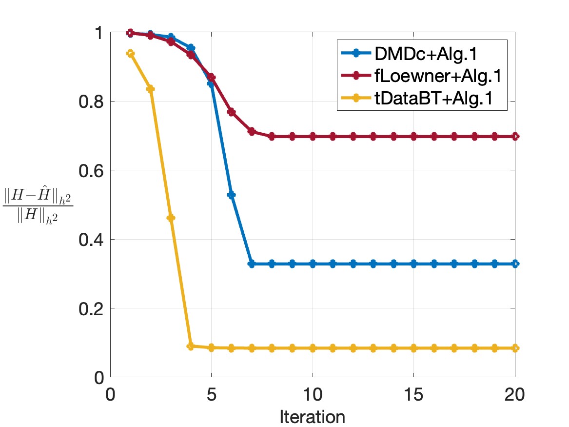
Figure 1: Convergence behavior for $N=102$ without noise.

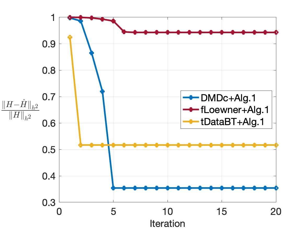
Figure 2: Convergence behavior for $N=102$ with noise.

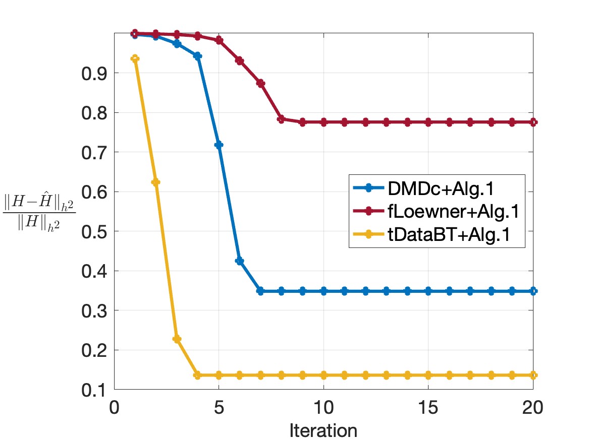
Figure 3: Convergence behavior for $N=510$ with noise.

VII Concluding remarks

In this paper, we propose a data-driven method for obtaining optimal ROMs in the $h^{2}$-norm sense for discrete-time linear systems (1). Theoretical and numerical analyses show that if the measurement data satisfy some assumptions, we can obtain better ROMs in terms of the $h^{2}$-norm than the outputs from the existing data-driven MOR methods. Furthermore, we have shown that even when traditional methods via system identification do not work, the proposed method can be used to obtain better ROMs that is better than the initial point.

We describe several future directions. The first is to extend the analysis to the continuous-time case. The second is to construct more computationally efficient algorithms for application to large-scale problems. The third is to extend (8) to an optimization problem on a Riemannian manifold. By extending it to a Riemannian manifold, as in [12] and [31], the reduced matrix $\hat{A}$ obtained at each iteration always satisfies stability, thus the stability constraint is no longer necessary.

References

- [1] B. Moore, “Principal component analysis in linear systems: Controllability, observability, and model reduction,” IEEE transactions on automatic control, vol. 26, no. 1, pp. 17–32, 1981.
- [2] C. Mullis and R. Roberts, “Synthesis of minimum roundoff noise fixed point digital filters,” IEEE transactions on Circuits and Systems, vol. 23, no. 9, pp. 551–562, 1976.
- [3] S. Gugercin and A. C. Antoulas, “A survey of model reduction by balanced truncation and some new results,” International Journal of Control, vol. 77, no. 8, pp. 748–766, 2004.
- [4] A. C. Antoulas, Approximation of large-scale dynamical systems. SIAM, 2005.
- [5] K. Willcox and J. Peraire, “Balanced model reduction via the proper orthogonal decomposition,” AIAA journal, vol. 40, no. 11, pp. 2323–2330, 2002.
- [6] Z. Bai, “Krylov subspace techniques for reduced-order modeling of large-scale dynamical systems,” Applied numerical mathematics, vol. 43, no. 1-2, pp. 9–44, 2002.
- [7] S. Gugercin, A. C. Antoulas, and C. Beattie, “ model reduction for large-scale linear dynamical systems,” SIAM journal on matrix analysis and applications, vol. 30, no. 2, pp. 609–638, 2008.
- [8] A. C. Antoulas, C. A. Beattie, and S. Gugercin, “Interpolatory model reduction of large-scale dynamical systems,” in Efficient modeling and control of large-scale systems. Springer, 2010, pp. 3–58.
- [9] P. Van Dooren, K. A. Gallivan, and P.-A. Absil, “H2-optimal model reduction of mimo systems,” Applied Mathematics Letters, vol. 21, no. 12, pp. 1267–1273, 2008.
- [10] A. Bunse-Gerstner, D. Kubalińska, G. Vossen, and D. Wilczek, “h2-norm optimal model reduction for large scale discrete dynamical mimo systems,” Journal of computational and applied mathematics, vol. 233, no. 5, pp. 1202–1216, 2010.
- [11] K. Sato, “Riemannian optimal model reduction of linear port-hamiltonian systems,” Automatica, vol. 93, pp. 428–434, 2018.
- [12] K. Sato, “Riemannian optimal model reduction of stable linear systems,” IEEE Access, vol. 7, pp. 14 689–14 698, 2019.
- [13] P. Rapisarda and H. L. Trentelman, “Identification and data-driven model reduction of state-space representations of lossless and dissipative systems from noise-free data,” Automatica, vol. 47, no. 8, pp. 1721–1728, 2011.
- [14] I. V. Gosea, S. Gugercin, and C. Beattie, “Data-driven balancing of linear dynamical systems,” SIAM Journal on Scientific Computing, vol. 44, no. 1, pp. A554–A582, 2022.
- [15] A. M. Burohman, B. Besselink, J. M. Scherpen, and M. K. Camlibel, “From data to reduced-order models via generalized balanced truncation,” IEEE Transactions on Automatic Control, 2023.
- [16] A. Mayo and A. Antoulas, “A framework for the solution of the generalized realization problem,” Linear algebra and its applications, vol. 425, no. 2-3, pp. 634–662, 2007.
- [17] S. Lefteriu and A. C. Antoulas, “A new approach to modeling multiport systems from frequency-domain data,” IEEE Transactions on Computer-Aided Design of Integrated Circuits and Systems, vol. 29, no. 1, pp. 14–27, 2009.
- [18] A. C. Ionita and A. C. Antoulas, “Matrix pencils in time and frequency domain system identification,” Control, Robotics and Sensors. Institution of Engineering and Technology, pp. 79–88, 2012.
- [19] A. C. Antoulas, S. Lefteriu, A. C. Ionita, P. Benner, and A. Cohen, “A tutorial introduction to the loewner framework for model reduction,” Model Reduction and Approximation: Theory and Algorithms, vol. 15, p. 335, 2017.
- [20] I. V. Gosea, C. Poussot-Vassal, and A. C. Antoulas, “Data-driven modeling and control of large-scale dynamical systems in the loewner framework: Methodology and applications,” in Handbook of Numerical Analysis. Elsevier, 2022, vol. 23, pp. 499–530.
- [21] B. Peherstorfer, S. Gugercin, and K. Willcox, “Data-driven reduced model construction with time-domain loewner models,” SIAM Journal on Scientific Computing, vol. 39, no. 5, pp. A2152–A2178, 2017.
- [22] Y. Liang, H. Lee, S. Lim, W. Lin, K. Lee, and C. Wu, “Proper orthogonal decomposition and its applications―part i: Theory,” Journal of Sound and vibration, vol. 252, no. 3, pp. 527–544, 2002.
- [23] J. N. Kutz, S. L. Brunton, B. W. Brunton, and J. L. Proctor, Dynamic mode decomposition: data-driven modeling of complex systems. SIAM, 2016.
- [24] J. L. Proctor, S. L. Brunton, and J. N. Kutz, “Dynamic mode decomposition with control,” SIAM Journal on Applied Dynamical Systems, vol. 15, no. 1, pp. 142–161, 2016.
- [25] I. Banno, S.-I. Azuma, R. Ariizumi, T. Asai, and J.-I. Imura, “Data-driven estimation and maximization of controllability gramians,” in 2021 60th IEEE Conference on Decision and Control (CDC). IEEE, 2021, pp. 5053–5058.
- [26] D. Vrabie, O. Pastravanu, M. Abu-Khalaf, and F. L. Lewis, “Adaptive optimal control for continuous-time linear systems based on policy iteration,” Automatica, vol. 45, no. 2, pp. 477–484, 2009.
- [27] F.-X. Orbandexivry, Y. Nesterov, and P. Van Dooren, “Nearest stable system using successive convex approximations,” Automatica, vol. 49, no. 5, pp. 1195–1203, 2013.
- [28] P. Van Dooren, K. A. Gallivan, and P.-A. Absil, “H_2-optimal model reduction with higher-order poles,” SIAM Journal on Matrix Analysis and Applications, vol. 31, no. 5, pp. 2738–2753, 2010.
- [29] V. Simoncini, “Computational methods for linear matrix equations,” siam REVIEW, vol. 58, no. 3, pp. 377–441, 2016.
- [30] M. Hamadi, K. Jbilou, and A. Ratnani, “A data-driven krylov model order reduction for large-scale dynamical systems,” Journal of Scientific Computing, vol. 95, no. 1, p. 2, 2023.
- [31] M. Obara, K. Sato, H. Sakamoto, T. Okuno, and A. Takeda, “Stable linear system identification with prior knowledge by riemannian sequential quadratic optimization,” IEEE Transactions on Automatic Control, accepted.
- [32] K.-w. E. Chu, “The solution of the matrix equations AXB- CXD= E AND (YA- DZ, YC- BZ)=(E, F),” Linear Algebra and its Applications, vol. 93, pp. 93–105, 1987.