Observables from classical black hole scattering in Scalar-Tensor theory of gravity from worldline quantum field theory

Abstract

In this article, we compute the two observables, impulse and waveform, in a black hole scattering event for the Scalar-Tensor theory of gravity with a generic scalar potential using the techniques of Worldline Quantum Field Theory. We mainly investigate the corrections to the above mentioned observables due to the extra scalar degree of freedom. For the computation of impulse, we consider the most general scenario by making the scalar field massive and then show that each computed diagram has a smooth massless limit. We compute the waveform for scalar and graviton up to 2PM, taking the scalar as massless. Furthermore, we discuss if the scalar has mass and how the radiation integrals get more involved than the massless case. We also arrive at some analytical results using stationary phase approximation. Interestingly, we also show that the $\lambda_{4}\varphi^{4}$ interaction vertex does not contribute to the radiation by showing that the integral has no non-zero finite value.

1 Introduction

The detection of gravitational waves through a network of ground-based laser-interferometers provide a new way of “listening” to the Universe in the high-frequency band LIGOScientific:2014oec ; LIGOScientific:2016aoc ; LIGOScientific:2016sjg ; LIGOScientific:2016vlm ; LIGOScientific:2017bnn ; LIGOScientific:2019hgc . A future space-based ones promises to open the low-frequency band, and also pulsar timing arrays are designed to explore gravitational waves at nano-hertz frequencies. In addition to providing astrophysical information, these observations will provide us a scope to test Einstein’s theory of general relativity in the strong-field, dynamical regime. While most tests so far constrain theory-agnostic deviations from general relativity (GR), current efforts aim at calculating waveform templates in specific modified gravity theories. The LIGO/VIRGO observations of black hole/Neutron star inspirals/mergers requires high precision analytical computations of classical potential and radiation coming out from the binary system Purrer:2019jcp . The high-precision computations are equivalent to the computations of scattering crosssection in elementary particle physics using the tools of Quantum Field Theory (QFT). Inspired by the QFT formalism, the perturbative quantum gravity formalism has been proven to be very efficient in investigating the classical gravitational interaction of black holes or Neutron stars.

In recent years, after the direct detection of gravitational waves (GW), renewed interest has spurred to test the legitimacy of General relativity (GR) directly at all possible length scales. One of the main reasons for this test is that although General Relativity (GR) has had remarkable success in describing classical gravity, including the phenomenal discovery of Gravitational waves (GW), the theory is incomplete. It is widely expected that there should be a consistent quantum theory of gravity, which is UV complete. Also, GR has not been able to explain the late-time acceleration of our universe: the phenomenon of dark energy. The late-time acceleration of the universe occurs at Hubble scales, a length scale much larger than the size of a gravitational wave emitter. Despite these shortcomings, GR and the Standard model of particle physics have been two bedrocks of theoretical physics. Hence, to incorporate the phenomenon of dark energy, Einstein’s GR needs to be adjusted so that, within reasonable limits, the adjusted theory yields the GR theory. There are two ways one can modify GR: adding higher curvature terms and adding extra gravitational degrees of freedom (DOF) stelle1 ; Alexeev:1996vs ; Lehebel:2018zga ; Volkov:2016ehx ; Kunz:2006ca . The simplest way to add extra DOF is by adding a scalar field along with the massless spin-2 graviton field Damour:1992we ; Horbatsch:2015bua ; Schon:2021pcv ; Rainer:1996gw ; DeFelice:2011bh . The addition of a scalar field is not ad-hoc but has several phenomenological motivations: The scalar field is considered one of the potential candidates of dark matter and can also explain the accelerating nature of our universe DeFelice:2011bh ; Gsponer:2021obj . Most importantly, adding an extra degree of freedom can have several effects on GW observables. The new degree of freedom can be observed as extra polarisation while studying the radiation emission during a scattering process. Extra polarisations induce rapid energy loss and can be measured in the propagation of GWs. In this paper, our main motivation is to find the scalar polarisation of the emission of radiation. Along with the observational motivations, the appearance scalar field also has theoretical motivation. After the discovery of General relativity, several attempts for a grand unification were made by Weyl and Kaluza weyl . Kaluza’s proposal, which was later known as the Kaluza-Klein (KK) theory, attempted to unify the Einstein-Maxwell theory by considering a five-dimensional spacetime with the fifth dimension compactified and behaving as a 4-vector. It plays the role of an electromagnetic potential. This idea led to the path towards formulating the Scalar-Tensor theory proposed by Jordan, where the scalar is coupled non-minimally to the tensor field. With the motivation to study the nature of the contribution coming from the scalar degree of freedom as an extra polarisation in radiation emission, one can explore novel amplitude techniques to find various GW observables.

Several classical approaches to investigate the binary inspirals and merger problem of black holes and neutron stars Blanchet:2013haa ; Schafer:2018kuf ; cite-key ; Pati:2000vt have surfaced in recent years. The gravitational classical potential and gravitational wave radiation up to 3PN has been investigated using the traditional methods in Tagoshi:2000zg ; Faye:2006gx ; Blanchet:2006gy ; Blanchet:2004ek ; Damour:2000ni ; Itoh:2003fy ; Boetzel:2019nfw ; Mishra:2013rna ; Kumar:2023bdf . Recent computations up to 4.5PN has been done in Fujita:2010xj ; Faye:2014fra ; Blanchet:2023sbv . Later, the investigation has been continued to the finite size effects of the binary system, including spins and tidal deformations PhysRevD.12.329 ; Kidder:1992fr ; Cho:2022syn ; Steinhoff:2007mb . Apart from General Relativity, those analysis are extensively done in modified gravity theories Zhang:2017srh ; Bernard:2022noq ; AbhishekChowdhuri:2022ora ; Zhang:2018prg ; Saffer:2018jmx ; Lin:2018ken ; Li:2022grj ; Shiralilou:2021mfl . In parallel with the traditional computations, a field-theoretic approach to the computation of classical potential and radiation in GR has emerged in recent years Goldberger:2004jt ; Goldberger:2009qd ; Kol:2007bc ; Goldberger:2007hy ; Porto:2016pyg ; Foffa:2013qca ; cite-key2 ; Levi:2018nxp . Furthermore, the EFT tools has been extensively used in modified gravity theories Bhattacharyya:2023kbh ; Diedrichs:2023foj ; Huang:2018pbu ; Bernard:2023eul .

Besides the inspiral problem, gravitational waves can be generated from scattering events. The study of classical gravitational scattering in post-Newtonian and post-Minkowskian regimes have been studied in hyp ; hyp1 ; hyp2 ; hyp3 ; hyp4 ; hyp5 ; hyp6 ; hyp7 ; hyp8 ; hyp9 ; hyp10 ; hyp11 ; hyp12 ; hyp13 ; hyp16 ; hyp14 ; Damour:2016gwp ; Bini:2017wfr ; Bini:2017xzy ; Damour:2017zjx ; Damour:2019lcq ; Bini:2020flp ; Bini:2020uiq ; Damour:2020tta ; Bini:2020rzn ; Bini:2021gat ; Bini:2022enm ; Damour:2022ybd ; Bini:2022wrq ; Rettegno:2023ghr ; Bini:2023fiz ; Ceresole:2023wxg . Inspired by the scattering amplitude computation in QFT and invited by Damour in Damour:2017zjx , the scattering of black holes/Neutron stars has gained interest in recent years by the amplitude community. A worldline Effective Field theory based on Post-Minkowskian (PM) expansion (where one has resumed PN expansion for every order in $G_{N}$) in Newton’s constant has been developed in Kalin:2020mvi for conservative binary dynamics. Later, the investigations continued with finite size effects, including spins and the tidal effects Bini:2020flp ; Cheung:2020sdj ; Kalin:2020lmz ; Haddad:2020que . The higher PM computations can be found in Kalin:2020fhe ; Dlapa:2021npj ; Dlapa:2021vgp ; Kalin:2022hph ; Jinno:2022sbr ; Dlapa:2022lmu ; Dlapa:2023hsl . In very recent past, the gravitational two-body problem has been investigated using more direct QFT techniques especially focused on on-shell methods of scattering amplitude PhysRevD.7.2317 ; Holstein:2004dn ; Neill:2013wsa ; Bjerrum-Bohr:2013bxa ; Luna:2017dtq ; Bjerrum-Bohr:2018xdl ; Kosower:2018adc . Those intricate methods have been extensively used in computing the classical gravitational potential in 2PM and 3PM Bjerrum-Bohr:2018xdl ; Cheung:2018wkq ; Cristofoli:2019neg ; Cheung:2020gyp ; Bern:2019nnu ; Bern:2019crd . The worldline EFT and scattering amplitude approaches gives same results and the question of efficiency depends on the taste. The prime question arises: Why do these two kindly different approaches give the same results? The gap between the two approaches has been bridged by Plefka et al. in Mogull:2020sak . It has been shown that the Feynmann-Schwinger representation of a graviton-dressed scalar propagator serves as the key to the scattering amplitude of two massive scalars. They provide a precise link between the scattering amplitude and the operator expectation value in the so-called Worldline Quantum Field Theory (WQFT). The formalism is similar to the formalism of Worldline Effective Field Theory (WEFT), but the main difference is that in WQFT, the worldline degrees of freedom (specifically the worldline fluctuations) are quantized. Using this method, the results from scattering amplitudes and PM-EFT have been investigated in non-spinning case first Jakobsen:2021smu and then generalized into spinning cases Jakobsen:2021lvp ; Jakobsen:2021zvh ; Jakobsen:2023ndj ; Jakobsen:2023hig . Further, the implementation has been done in higher PM order, including the tidal effects also Jakobsen:2023pvx . The WQFT formalism has also been used to investigate the phenomena of gravitational lensing Bastianelli:2021nbs . Eventually, the classical double copy relation has been studied using WQFT in Diaz-Jaramillo:2021wtl ; Comberiati:2022cpm .

All in all, till now, most of the scattering events have been investigated in GR. We take the step to compute the observables in a non-GR theory, primarily focused on the massive Scalar-Tensor theory of gravity where we have non-trivial cubic and quartic scalar potential. Our bigger goal is to inspect, apart from the mass of the scalar, whether we can put constraints on the cubic ($\lambda_{3}$) and quartic coupling ($\lambda_{4}$) from gravitational wave observations. To do this, we take the primary step forward and compute the two main observables in a scattering event: impulse and waveform. The impulse is directly connected to the scattering angle, from which one can get information about the bound state of the system through the connection with the EOB prescription Buonanno:1998gg . Rather, the more interesting part comes from the waveform computation, which is the key to computing the gravitational wave phase. In the game of waveform computation from WQFT, the main technical challenge is to compute the integrals. At this point, we make explicit computations of massive waveform integrals and propose methods for handling such integrals analytically, which are, to the best of our knowledge, new results.

The paper is organized as follows: In Section (2), we briefly review the WQFT formalism and summarize the main results of the formalism in Mogull:2020sak . In Section (3), we mention the changes in the results of Mogull:2020sak due to the presence of an extra massive scalar degree of freedom. Then, we derive all the worldline Feynman rules from the scalar and graviton. In Section (4), we use the Feynman rules derived earlier to compute the corrections of impulse due to the scalar field. We compute all the Feynman diagrams involving the self-interaction of the scalar field and scalar-graviton interaction. In Section (5) we start computing the radiation integrands and then move to the computation of time-domain waveform, assuming the scalar field is massless. In Section (6), we first discuss how the massive radiation integral gets complicated due to the presence of a more involved phase factors. Next, we list all the massive radiation integrands. We propose a method to compute those integrals using the stationary phase method, which is a very good approximation in the limit $|x|\to\infty$. We computed all the massive integrals in the stationary phase approximation and discussed the underlying subtleties. In Appendix (A), we give a short derivation of the worldline effective action in the presence of extra scalar degrees of freedom. In Appendix (B), we discuss the connection between impulse and the scattering amplitude through the Eikonal phase. In Appendix (C), (D), (E), we give some more details about the integrals used in the main text. In Appendix (F), we provide another method of approximating the worldline radiation integral using large velocity approximation.

Notations and Conventions:
•   Metric sign convention: ($+,-,-,-$).
•   All computations are done in the unit where, $(c,\hbar)=1$.
•   The impact parameter $b$ is purely spacelike, $b^{2}=b^{\mu}b_{\mu}=-|b|^{2}$.
•   Black hole velocity parametrization: $v_{1}=(\gamma,\gamma\beta,0,0)$, $v_{2}=(1,0,0,0)$.
•   Planck mass: $m_{p}=\frac{1}{\sqrt{8\pi G_{N}}}$, where $G_{N}$ is Newton’s constant.

2 A quick tour to worldline quantum field theory

In this section, we briefly summarize the results of the Worldline Quantum Field Theory (WQFT) approach to the scattering problem. In Mogull:2020sak , precise correspondence has been derived between the scalar-graviton S-matrix element and the one-point functions of the worldline operators. In this string-inspired approach, one maps black hole scattering in worldline theory to field scattering in the field theory approach. Using the gravitationally dressed Green’s functions, one can write S-matrix elements as the expectation value of operators present in the worldline theory.

Now, for spinless blackholes in GR, the action can be written in the EFT framework as ,

$$S=S_{EH}+S_{gf}+\sum_{i}S_{pm}^{i}\,,$$

where $S_{EH}$ is the usual Einstein-Hilbert action with $S_{gf}$ is the gauge-fixing action, which in the weak field approximation is given by,

$$S_{gf}=\int d^{D}x\Big{(}\partial_{\nu}h^{\mu\nu}-\frac{1}{2}\partial^{\mu}h^{\nu}_{\nu}\Big{)}^{2}\,.$$

This imposes the de-Donder gauge condition. Now, for an extended object, the worldline action consists of the Wilson coefficients $c_{v}$ and $c_{R}$ as follows,

$$S_{pm}=-m\int d\tau+c_{R}\int d\tau R(x)+c_{v}\int d\tau R_{\mu\nu}(x)\dot{x}^{\mu}\dot{x}^{\nu}+\cdots\,.$$ (1)

In our paper, we will drop the second and third terms above to remove the complicacy due to the finite-size effects. In principle, there will be an infinite tower of terms consisting of higher-order derivatives of metric represented as dots.

Now, assuming a fixed background, we can write Green’s function of the field theory as a two-point correlator :

$$G_{i}(x,x^{\prime})=\mathcal{Z}_{i}^{-1}\int\mathcal{D}[\phi_{i}]\phi_{i}(x)\phi_{i}^{\dagger}(x^{\prime})e^{iS_{i}},$$ (2)

where, $S_{i}=\int d^{D}x\sqrt{-g}(g^{\mu\nu}\partial_{\mu}\phi_{i}^{\dagger}\partial_{\nu}\phi_{i}-m^{2}\phi_{i}^{\dagger}\phi_{i}-\zeta R\phi_{i}^{\dagger}\phi_{i})$.

To this end, we have to integrate out certain field degrees of freedom with respect to a relevant scale of the problem. This will give rise to the one-loop effective action, which can be represented by a worldline path integral Strassler:1992zr ; Feal:2022iyn ; Ahmadiniaz:2022yam . Then, from this path integral, we can identify the point particle action in the background of $h_{\mu\nu}$. Now for our interest, we evaluate the S-matrix element of two scalars with or without a final state graviton in certain classical limit as,

$$\langle\Omega|T\{h_{\mu\nu}\phi_{1}(x_{1})\phi_{1}^{\dagger}(x_{1}^{\prime})\phi_{2}(x_{2})\phi_{2}^{\dagger}(x_{2}^{\prime})\}|\Omega\rangle$$ (3)

$$=\mathcal{Z}_{i}^{-1}\int\mathcal{D}[h_{\mu\nu},\phi_{i}]h_{\mu\nu}(x)\prod_{i=1}^{2}\phi_{i}(x_{i})\phi_{i}^{\dagger}(x_{i}^{\prime})e^{iS^{\prime}}\,.$$ (4)

Fourier transforming this relation and using LSZ reduction in the $\hbar\rightarrow 0$ limit we get Mogull:2020sak ,

$$\langle\phi_{1}\phi_{2}(+h)|S|\phi_{1}\phi_{2}\rangle$$ (5)

$$=\mathcal{Z}^{-1}\int d^{D}[x_{i},x_{i}^{\prime},x]e^{ip\cdot x-ip_{i}^{\prime}\cdot x_{i}^{\prime}-ik\cdot x}\times\int[\mathcal{D}h_{\alpha\beta}]\,\epsilon^{\mu\nu}(k)h_{\mu\nu}(x)\prod_{i=1}^{2}G_{i}(x_{i},x_{i}^{\prime})e^{iS_{EH}+S_{gf}}\bigg{|}_{\textrm{Amputated,connected}}\,.$$ (6)

The study of the S-matrices consists of applying the LSZ reduction. Cutting the propagators on external legs, we convert Correlators into S-matrices and send the external legs to infinity, where they interact weakly. We put the scalar legs on-shell, and the integration over the finite time domain extends $\tau\in(-\infty,\infty)$. The key relation connecting the QFT form factor to the WQFT correlator is given by Mogull:2020sak , white!10 black

$$\begin{split}\tikzmarkin[disableroundedcorners=true]{g1}(0.1,-0.6)(-0.1,0.8)\frac{\Xi(b,v;\{\epsilon^{l},k_{l}\})}{\Xi_{0}}=\delta\Bigg{(}\sum_{l=1}^{N}k_{l}\cdot v\Bigg{)}\exp\Big{(}{\sum_{l=1}^{N}k_{l}\cdot b}\Big{)}\mathcal{F}(p,p^{\prime}|\{\epsilon^{l},k_{l}\})\tikzmarkend{g1}\end{split}$$ (7)

where,

$$\Xi(b,v;\{\epsilon^{l},k_{l}\})=\int\mathcal{D}[x]\int\mathcal{D}[a,b,c]\exp[-i\int d\sigma\Big{[}\frac{1}{4}g_{\mu\nu}(\dot{x}^{\mu}\dot{x}^{\nu}+a^{\mu}a^{\nu}+b^{\mu}c^{\nu})\Big{]}.$$ (8)

Having the gravitationally dressed propagator in momentum space, we put the external scalar legs on-shell to perform the LSZ reduction. Effectively, it can be represented as,

$$\begin{split}\mathcal{F}(p,p^{\prime}|\{\epsilon^{l},k_{l}\})=\langle p^{\prime}|\prod_{i=1}^{N}\epsilon_{i}\cdot h(k_{i})|p\rangle=\begin{minipage}[h]{21.68231pt} \vspace{-1 cm}\scalebox{0.4}{\includegraphics{fey_1.pdf}}\end{minipage}\,.\end{split}$$ (9)

For details, we refer the reader to Mogull:2020sak . In the following section, we will discuss how to derive the Feynman rules for the scattering events of two black holes (including extra scalar modes), which are considered to be point-like objects and, hence, spinless.

3 Derivation of the Feynman rules

One of the key ingredients to compute the observables in a scattering problem is the partition function. We compute the partition function for a binary system in the Scalar-Tensor theory of gravity with a generic scalar potential. The gravitational is given by,

$$\begin{split}S_{g}=\int d^{4}x\sqrt{-g}[\frac{m_{p}^{2}}{2}R+\frac{1}{2}{g}^{\alpha\beta}\partial_{\alpha}{\varphi}\partial_{\beta}{\varphi}-\frac{1}{2}m^{2}{\varphi}^{2}-\lambda_{3}m_{p}\,\varphi^{3}-\lambda_{4}{\varphi}^{4}]\in S_{EH}+S_{scalar}.\end{split}$$ (10)

In this theory, the mass of the point particle which is the avatar of the scalar field $\phi_{i}$, is not constant but rather depends on the extra scalar degree of freedom $\varphi$ eardley . Hence the matter action has the following form,

$$\begin{split}S_{m}=\sum_{i=1}^{2}\int d^{4}x\sqrt{-g}(g^{\mu\nu}\partial_{\mu}\phi_{i}^{\dagger}\partial_{\nu}\phi_{i}-m_{i}(\varphi)^{2}\phi_{i}^{\dagger}\phi_{i}-\zeta R\phi_{i}^{\dagger}\phi_{i})\,.\end{split}$$ (11)

Therefore, the WQFT partition function takes the form ,

$$\begin{split}{Z}_{\textrm{WQFT}}=\mathcal{N}\times\int\mathcal{D}[h_{\mu\nu},\,{\varphi}]\int\mathcal{D}[x_{i},a_{i},b_{i},c_{i}]e^{iS_{g}}\exp\Big{\{}-i\sum_{i=1}^{2}\int d\tau_{i}\frac{m_{i}(\varphi)}{2}g_{\mu\nu}(\dot{x}_{i}^{\mu}\dot{x}_{i}^{\nu}+a_{i}^{\mu}a_{i}^{\nu}+b_{i}^{\mu}b_{i}^{\nu})\Big{\}}\end{split}$$ (12)

where, $a_{i},b_{i}$ s are Lee-Yang Ghost and can be ignored in the classical limit. Therefore, the $n$-body partition function (non-spinning) in WQFT can be written as,

$$\begin{split}Z_{\textrm{WQFT}}^{(n)}=\mathcal{N}\int\mathcal{D}h_{\mu\nu}\mathcal{D}\varphi\,e^{iS_{EH}+iS_{scalar}}\Big{(}\prod_{i=1}^{n}\mathcal{D}x_{i}\,e^{iS_{pm}^{i}}\Big{)}\,.\end{split}$$ (13)

It has been noticed that the partition function is related to the Eikonal phase $\chi$ by the following exponentiation Amati:1990xe ; Mogull:2020sak .

$$\begin{split}Z_{\textrm{WQFT}}:=e^{i\chi}\,.\end{split}$$ (14)

Now $\chi$ can be calculated by computing the connected Feynmann diagrams. In order to compute the path integral in (13) one could start by demanding a gravitational field is a fluctuation over Minkowski space, i.e., one can decompose the metric $g_{\mu\nu}$ as,

$$\begin{split}g_{\mu\nu}=\eta_{\mu\nu}+\frac{h_{\mu\nu}}{m_{p}}.\end{split}$$ (15)

and, eventually, the worldline degree of freedom can be expanded as,

$$\begin{split}x^{\mu}(\tau)=b^{\mu}+v^{\mu}\tau+z^{\mu}(\tau)\end{split}$$ (16)

where, $z^{\mu}(\tau)$ is the worldline fluctuation about the straightline geodesic. Once we have the well-defined partition function, one could compute the classical observables as a correlation function in WQFT.

$$\begin{split}\mathcal{O}(b_{i},v_{i}):=\langle\hat{\mathcal{O}}(\hat{x},\hat{h}_{\mu\nu},\hat{\varphi})\rangle=\frac{1}{Z^{(n)}_{\textrm{WQFT}}}\int\mathcal{D}h_{\mu\nu}\mathcal{D}\varphi\,e^{iS_{EH}+iS_{scalar}}\Big{(}\prod_{k=1}^{n}\mathcal{D}x_{k}e^{iS_{pm}^{k}}\Big{)}\mathcal{O}(x_{i},h,\varphi)\end{split}$$ (17)

where the worldline action can be written in Polyakov form. The point particle action has the following form,

$$\begin{split}S_{pm}=-\sum_{k=1}^{n}\int_{-\infty}^{\infty}d\tau_{k}\frac{m_{k}(\varphi)}{2}(g_{\mu\nu}\dot{x}^{\mu}_{k}\dot{x}^{\nu}_{k}+1).\end{split}$$ (18)

We intend to compute the two main observables, impulse and waveform, schematically defined as,

$$\begin{split}\langle\hat{h}_{\mu\nu}(k),\hat{\varphi}(k),\hat{z}^{\mu}(\omega)\rangle=Z_{\textrm{WQFT}}^{-1}\int\mathcal{D}h_{\mu\nu}\mathcal{D}\varphi\,e^{iS_{EH}+iS_{scalar}}\Big{(}\prod_{k=1}^{2}\mathcal{D}x_{k}e^{iS_{pm}^{k}}\Big{)}\{h_{\mu\nu}(k),\varphi(k),z^{\mu}(\omega)\}\,.\end{split}$$ (19)

Before going to the computations of the partition function, we first derive all the Feynman rules. In Scalar-Tensor theory, the violation of the equivalence principle automatically implies that the mass of the binaries depends on the extra gravitational polarisation ${\varphi}$. As there is a self-interaction term so one can expand $m_{a}(\varphi)$ around one of the chosen vacuums ${\varphi}_{0}$, which for our case is zero, as,

$$\begin{split}m_{a}({\varphi})=m_{a}(0)\Big{\{}1+s_{a}\varphi+g_{a}\varphi^{2}+\mathcal{O}(\varphi^{3})\Big{\}}.\end{split}$$ (20)

In order to derive the Feynman rules it would be better to decompose the fields ($\chi(x)\in(h_{\mu\nu},\varphi)$) in their Fourier mode assuming the black hole worldline has following the fluctuation due to the radiation reaction: $x_{(i)}^{\mu}=b_{(i)}^{\mu}+v_{(i)}^{\mu}\tau+z_{(i)}^{\mu}(\tau)$. where $z_{i}^{\mu}(\tau)$ is the worldline fluctuations about the straight line geodesic. Now, we expand the point particle action at different orders in $z$ to get the worldline vertices. In our theory we have gravitational field ($h_{\mu\nu}$) and scalar field (${\varphi}$). One can decompose the fields in Fourier modes, when it couples with worldline, as,

$$\begin{split}&\chi(x_{i})=\int_{k}e^{ik\cdot(b_{i}+v_{i}\tau+z_{i})}\chi(-k)\,.\end{split}$$ (21)

Now, expanding the exponential at different orders in $z$ and is given by,

$$\begin{split}\chi(x_{i})=\int_{k}e^{ik\cdot(b_{i}+v_{i}\tau)}\prod_{n=0}^{\infty}\frac{i^{n}}{n!}(k\cdot z)^{n}\chi(-k)\,.\end{split}$$ (22)

Again, we decompose the worldline fluctuations as,

$$\begin{split}z^{\mu}(\tau)=\int_{\omega}e^{i\omega\tau}z^{\mu}(-\omega)\,.\end{split}$$ (23)

From the quadratic part of Einstein-Hilbert action, one can identify the graviton propagator as,

$$\langle h_{\mu\nu}(x_{1})h_{\rho\sigma}(x_{2})\rangle\equiv\begin{minipage}[h]{52.03227pt} \vspace{4pt} \scalebox{1.8}{\includegraphics[width=433.62pt]{graviton_propagator_1.pdf}} \end{minipage}\hskip 34.14322pt=iP_{\mu\nu;\rho\sigma}\int_{k}\frac{e^{-ik\cdot(x_{1}-x_{2})}}{k^{2}+i\epsilon}$$ (24)

where,

$$\begin{split}P_{\mu\nu,\rho\sigma}=\eta_{\mu\rho}\eta_{\nu\sigma}+\eta_{\mu\sigma,\nu\rho}-\frac{1}{2}\eta_{\mu\nu}\eta_{\rho\sigma}.\end{split}$$ (25)

and propagator for the scalar degrees of freedom has the following form,

$$\begin{split}\langle\varphi(x_{1})\varphi(x_{2})\rangle\equiv\begin{minipage}[h]{52.03227pt} \vspace{4pt} \scalebox{1.8}{\includegraphics[width=433.62pt]{scalar_propagator_1.pdf}} \end{minipage}\hskip 36.98866pt=i\int_{k}\frac{e^{-ik\cdot(x_{1}-x_{2})}}{k^{2}-m^{2}+i\epsilon}\,.\end{split}$$ (26)

Apart from the field degrees of freedom, we have another dynamical degree of freedom: worldline fluctuations $z^{\mu}(\omega)$. One can identify the propagator by inspecting the quadratic part of the worldline action (18).

$$\begin{split}S_{\textrm{pm}}=-m(\varphi_{0})\int d\tau\Big{[}1+\eta_{\mu\nu}v^{\mu}\dot{z}^{\nu}+\frac{1}{2}\eta_{\mu\nu}\dot{z}^{\mu}\dot{z}^{\nu}\Big{]}\end{split}$$ (27)

The propagator of $z^{\mu}$ can be identified from the quadratic part of (27).

$$\begin{split}\Big{\langle}z^{\mu}(\tau_{1})z^{\nu}(\tau_{2})\Big{\rangle}\equiv\begin{minipage}[h]{52.03227pt} \vspace{4pt} \scalebox{1.6}{\includegraphics[width=433.62pt]{worldline_propagator.pdf}} \end{minipage}\hskip 28.45274pt=-i\frac{\eta^{\mu\nu}}{m}\int_{\omega}\frac{e^{-i\omega(\tau_{1}-\tau_{2})}}{(\omega\pm i\epsilon)^{2}}\,.\end{split}$$ (28)

Now, we are in a position to derive the worldline Feynman rules. The key ingredient is the worldline action $S_{\textrm{pm}}$ in (18).

$$\begin{split}S_{\textrm{pm}}\Big{|}_{\textrm{int.}}\in\int d\tau\Big{[}\Big{(}-\frac{m_{a}}{2}-\frac{m_{a}s_{a}}{2}\varphi-\frac{m_{a}g_{a}}{2}\varphi^{2}\Big{)}(\eta_{\mu\nu}+\frac{1}{m_{p}}h_{\mu\nu})(v^{\mu}+\dot{z}^{\mu})(v^{\nu}+\dot{z}^{\nu})\Big{]}\,.\end{split}$$ (29)

We can rewrite (22) by inserting the Fourier mode of the worldline fluctuation in the following way.

$$\begin{split}\chi=\sum_{m=0}^{\infty}\frac{i^{m}}{m!}\int_{k,\omega_{1},...,\omega_{m}}e^{ik\cdot b}e^{i(k\cdot v+\sum_{i=1}^{m}\omega_{i})\tau}\prod_{i=1}^{m}[k\cdot z(-\omega_{i})]\chi(-k).\end{split}$$ (30)

The expansion in (30) helps to derive the Feynman rules upto $\mathcal{O}(z^{j})$. Now, we list down the Feynman rules coming from the scalar-worldline interaction:

Vertex for scalar field:

• $\mathcal{O}{(z^{0})}:-i\frac{m_{a}s_{a}}{m_{p}}\,e^{ik\cdot b_{a}}\,\hat{\delta}(k\cdot v)\rightarrow\begin{minipage}[h]{52.03227pt} \vspace{4pt} \scalebox{1.6}{\includegraphics[width=433.62pt]{feynmann_2_1.pdf}} \end{minipage}$

• $\mathcal{O}(z):\frac{m_{a}s_{a}}{2m_{p}}\,e^{ik\cdot b}\,\hat{\delta}(k\cdot v+\omega)(2\omega v_{\rho}+k_{\rho})\rightarrow\begin{minipage}[h]{52.03227pt} \vspace{4pt} \scalebox{1.6}{\includegraphics[width=433.62pt]{feynmann_3_1.pdf}} \end{minipage}$

• $\mathcal{O}(z):-\frac{m_{a}g_{a}}{2m_{p}^{2}}e^{i(k_{1}+k_{2})\cdot b_{a}}\hat{\delta}(k_{1}\cdot v_{1}+k_{2}\cdot v_{1}+\omega)\{(k_{1\rho}+k_{2\rho})v^{\mu}v^{\nu}+2\omega v^{(\mu}\delta_{\rho}^{\nu)}\}\rightarrow\begin{minipage}[h]{52.03227pt} \vspace{4pt} \scalebox{1.8}{\includegraphics[width=433.62pt]{phi_2_z_1.pdf}} \end{minipage}$

• $\mathcal{O}{(z^{2})}:i\frac{m_{a}s_{a}}{2m_{p}}\,e^{ik\cdot b_{a}}\,\hat{\delta}(k\cdot v+\omega_{1}+\omega_{2})(\frac{1}{2}k_{\rho_{1}}k_{\rho_{2}}+\omega_{1}k_{\rho_{2}}v_{\rho_{1}}+\omega_{2}k_{\rho_{1}}v_{\rho_{2}}+\omega_{1}\omega_{2}\delta_{\rho_{1}\rho_{2}})\rightarrow\begin{minipage}[h]{52.03227pt} \vspace{4pt} \scalebox{1.6}{\includegraphics[width=433.62pt]{phi_z_2.pdf}} \end{minipage}$

Vertex for gravitational field:

• $\mathcal{O}{(z^{0})}:-i\frac{m_{a}}{2m_{p}}\,e^{ik\cdot b_{a}}\,\hat{\delta}(k\cdot v)v_{a}^{\mu}v_{a}^{\nu}\rightarrow\begin{minipage}[h]{52.03227pt} \vspace{4pt} \scalebox{1.6}{\includegraphics[width=433.62pt]{h_z_0.pdf}} \end{minipage}$

• $\mathcal{O}(z^{1}):\frac{m_{a}}{2m_{p}}\,e^{ik\cdot b}\,\hat{\delta}(k\cdot v+\omega)(2\omega v^{(\mu}\delta^{\nu)}_{\rho}+v^{\mu}v^{\nu}k_{\rho})\rightarrow\begin{minipage}[h]{52.03227pt} \vspace{4pt} \scalebox{1.6}{\includegraphics[width=433.62pt]{h_z_1.pdf}} \end{minipage}$

• $\mathcal{O}{(z^{2})}:i\frac{m_{a}}{m_{p}}\,e^{ik\cdot b_{a}}\,\hat{\delta}(k\cdot v+\omega_{1}+\omega_{2})(\frac{1}{2}k_{\rho_{1}}k_{\rho_{2}}v^{\mu}v^{\nu}+\omega_{1}k_{\rho_{2}}v^{(\mu}\delta^{\nu)}_{\rho_{1}}+\omega_{2}k_{\rho_{1}}v^{(\mu}\delta^{\nu)}_{\rho_{2}}+\omega_{1}\omega_{2}\delta^{(\mu}_{\rho_{1}}\delta^{\nu)}_{\rho_{2}})\rightarrow\begin{minipage}[h]{52.03227pt} \vspace{4pt} \scalebox{1.6}{\includegraphics[width=433.62pt]{h_z_2.pdf}} \end{minipage}$

4 Computation of impulse

In this section, we will compute the impulse in a purely conservative setting. We mainly focus on the corrections to the impulse coming from the purely scalar degree of freedom or the interaction between scalar and graviton. The impulse is defined as,

$$\begin{split}\Delta p^{\mu}_{i}=m_{i}\int_{-\infty}^{\infty}d\tau_{i}\Big{\langle}\frac{d^{2}z_{i}^{\mu}}{d\tau_{i}^{2}}\Big{\rangle}_{\text{WQFT}}=-m_{i}\omega^{2}\langle z_{i}^{\mu}(\omega)\rangle|_{\text{WQFT}}\Big{|}_{\omega=0}.\end{split}$$ (31)

Now we will compute (31) order by order in Newton’s constant $G_{N}$ upto 2PM order.

•   The simplest diagram at 1 PM order consists only of a scalar field that has the following form,

$$\begin{split}\Delta p_{1}^{\mu}=\begin{minipage}[h]{52.03227pt} \vspace{4pt} \scalebox{1.6}{\includegraphics[width=433.62pt]{z_1_1.pdf}} \end{minipage}\hskip 28.45274pt&=-i\frac{m_{1}s_{1}m_{2}s_{2}}{4m_{p}^{2}}\int_{k_{1},k_{2}}e^{ik_{1}\cdot b_{1}+ik_{2}\cdot b_{2}}\frac{\hat{\delta}(k_{2}\cdot v_{2})\hat{\delta}(\omega-k_{1}\cdot v_{1})}{k_{1}^{2}-m^{2}}\hat{\delta}^{(4)}(k_{1}+k_{2})\\ &\hskip 256.0748pt\times(k_{1}^{\mu}+2\omega v_{1}^{\mu})\Big{|}_{\omega=0}\,,\\ &=-i\frac{m_{1}s_{1}m_{2}s_{2}}{4m_{p}^{2}}\int_{k}e^{ik\cdot(b_{1}-b_{2})}\frac{k^{\mu}\hat{\delta}(k_{1}\cdot v_{1})\hat{\delta}(k_{2}\cdot v_{2})}{k^{2}-m^{2}}\,,\\ &=-\frac{m_{1}s_{1}m_{2}s_{2}}{4m_{p}^{2}}\frac{\partial}{\partial b_{1\mu}}\underbrace{\int_{k}e^{ik\cdot(b_{1}-b_{2})}\frac{\delta(k\cdot v_{1})\hat{\delta}(k\cdot v_{2})}{k^{2}-m^{2}}}_{\chi}\,.\end{split}$$ (32)

To do this integral, we need to choose the coordinates suitably. We study the dynamics from the frame of the second black hole. Hence in the mentioned parametrization of velocities satisfying $v_{1}\cdot v_{2}=\gamma$. Hence,

$$\begin{split}\chi&=\frac{m_{1}m_{2}s_{1}s_{2}}{4m_{p}^{2}}\int_{k}\frac{\hat{\delta}{(\gamma k^{(0)}-\gamma\beta k^{(1)})}\hat{\delta}(k^{0})}{k^{2}-m^{2}}e^{ik\cdot b}\,,\\ &=-\frac{m_{1}m_{2}s_{1}s_{2}}{4m_{p}^{2}\sqrt{\gamma^{2}-1}}\int_{\tilde{k}}\frac{e^{-i\tilde{k}\cdot b}}{\tilde{k}^{2}+m^{2}}=-\frac{m_{1}m_{2}s_{1}s_{2}}{4m_{p}^{2}\sqrt{\gamma^{2}-1}}K_{0}(m|b|)\,.\end{split}$$ (33)

Therefore, gray!10 black

$$\begin{split}\tikzmarkin[disableroundedcorners=false]{e}(0.1,-0.55)(-0.1,0.8)\Delta p_{1}^{\mu}&=\frac{m_{1}m_{2}s_{1}s_{2}}{4m_{p}^{2}\sqrt{\gamma^{2}-1}}\frac{b^{\mu}}{|b|}mK_{1}(m|b|)\,.\tikzmarkend{e}\end{split}$$ (34)

In the massless limit the impulse took the form,

$$\begin{split}\Delta p_{1}^{\mu}\Big{|}_{m\to 0}=\frac{m_{1}m_{2}s_{1}s_{2}}{4m_{p}^{2}\sqrt{\gamma^{2}-1}}\frac{b^{\mu}}{|b|^{2}}.\end{split}$$ (35)

•   One more diagram comes from the self-interaction vertex, which contributes at 1 PM order.

$$\begin{split}\mathcal{O}(z^{1},\lambda_{2}^{1}):-\lambda_{3}m_{p}\int d^{4}x\,\varphi(x)^{3}.\end{split}$$ (36)

Then,

$$\begin{split}\Delta p_{1}^{\mu}=\begin{minipage}[h]{52.03227pt} \scalebox{1.5}{\includegraphics[width=433.62pt]{z_1_4.pdf}} \end{minipage}&=-i\lambda_{3}\frac{m_{1}s_{1}}{2}\times\Big{(}\frac{m_{2}s_{2}}{2m_{p}}\Big{)}^{2}\int_{k_{i}}\hat{\delta}^{(4)}\Big{(}\sum_{i}k_{i}\Big{)}\frac{k_{1}^{\mu}\hat{\delta}(k_{1}\cdot v_{1})\hat{\delta}(k_{2}\cdot v_{2})\hat{\delta}(k_{3}\cdot v_{2})}{\prod_{i=1}^{3}(k_{i}^{2}-m^{2})}e^{ik_{1}\cdot b_{1}}e^{i(k_{2}+k_{3})\cdot b_{2}}\,,\\ &=-i\lambda_{3}\frac{m_{1}s_{1}}{2}\times\Big{(}\frac{m_{2}s_{2}}{2m_{p}}\Big{)}^{2}\int_{k_{1,2}}\frac{k_{1}^{\mu}\hat{\delta}(k_{1}\cdot v_{1})\hat{\delta}(k_{2}\cdot v_{2})\hat{\delta}(k_{1}\cdot v_{2})}{(k_{1}^{2}-m^{2})(k_{2}^{2}-m^{2})[(k_{1}+k_{2})^{2}-m^{2}]}e^{ik_{1}\cdot(b_{1}-b_{2})}\,.\end{split}$$ (37)

No using the proper velocity parametrization and using the integral results derived in Bhattacharyya:2023kbh we will get,

$$\begin{split}\Delta p_{1}^{\mu}&=-i\lambda_{3}\frac{m_{1}s_{1}}{2}\times\Big{(}\frac{m_{2}s_{2}}{2m_{p}}\Big{)}^{2}\frac{1}{\gamma\beta}\int d^{2}l_{1}\frac{l_{1}^{\mu}e^{il_{1}\cdot b}}{(\vec{l}_{1}^{2}+m^{2})|\vec{l}_{1}|}\arctan\Big{(}\frac{|\vec{l}_{1}|}{2m}\Big{)}\,,\\ &=\lambda_{3}\frac{m_{1}s_{1}}{2}\times\Big{(}\frac{m_{2}s_{2}}{2m_{p}}\Big{)}^{2}\frac{1}{\gamma\beta}\frac{\partial}{\partial b_{1\mu}}\underbrace{\int_{0}^{\infty}dl_{1}\,\frac{J_{0}(|b|l_{1})}{l_{1}^{2}+m^{2}}\arctan\Big{(}\frac{l_{1}}{2m}\Big{)}}_{I_{3}(m,b)}\,,\\ &=\lambda_{3}\frac{m_{1}s_{1}}{2}\times\Big{(}\frac{m_{2}s_{2}}{2m_{p}}\Big{)}^{2}\frac{1}{\gamma\sqrt{\gamma^{2}-1}}\frac{b^{\mu}}{|b|}\frac{\partial I_{3}(m,|b|)}{\partial|b|}\,.\end{split}$$ (38)

Finally, we get, gray!10 black

$$\tikzmarkin[disableroundedcorners=false]{c}(0.3,-0.6)(-0.1,0.8)\Delta p_{1}^{\mu}=\lambda_{3}\frac{m_{1}s_{1}}{2}\times\Big{(}\frac{m_{2}s_{2}}{2m_{p}}\Big{)}^{2}\frac{1}{\gamma\sqrt{\gamma^{2}-1}}\frac{b^{\mu}}{|b|}\frac{\partial I_{3}(m,|b|)}{\partial|b|}\tikzmarkend{c}\,.$$ (39)

In the massless limit the contribution gives,

$$\begin{split}\Delta p_{1}^{\mu}\Big{|}_{m\to 0}=-\lambda_{3}\frac{\pi m_{1}s_{1}}{2}\times\Big{(}\frac{m_{2}s_{2}}{4m_{p}}\Big{)}^{2}\frac{1}{\gamma\sqrt{\gamma^{2}-1}}\frac{b^{\mu}}{|b|}\,.\end{split}$$ (40)

Then the total impulse (due to the scalar field) at 1PM order is the sum of (34) and (39)  Next we extend this computation to 2PM order.

•   At $\mathcal{O}(z)$ simplest diagram comes from the graviton-scalar interaction vertex:

$$\begin{split}\mathcal{O}(z):-\frac{1}{2}m^{2}\int d^{4}x\frac{h}{2m_{p}}\varphi^{2}\,.\end{split}$$ (41)

The corresponding contribution to the impulse is given by ,

$$\begin{split}\Delta p_{1}^{\mu}&=\begin{minipage}[h]{52.03227pt} \scalebox{1.5}{\includegraphics[width=433.62pt]{z_1_2.pdf}} \end{minipage}\hskip 19.91684pt\propto\underbrace{P_{\rho\rho,\sigma\delta}\,v_{1}^{\sigma}v_{1}^{\delta}}_{0}\,.\end{split}$$ (42)

Then, from (25), it is evident that this contribution vanishes. Note that the external fluctuation ($z^{\mu}$) is connected with $h_{\mu\nu}\,.$ But there can be another diagram where it can be connected with either of the scalar fields. In those cases, $P_{\rho\rho,\sigma\delta}\,v_{2}^{\sigma}v_{2}^{\delta}$ will appear and from (25) again it is evident that it vanishes.

•   Now, we concentrate on the scalar interaction diagrams. We compute the contribution to the impulse at 2PM order coming from the scalar self-interaction vertex:

$$\begin{split}\mathcal{O}(z^{1}):-\lambda_{4}\int d^{4}x\,\varphi^{4}(x)\,.\end{split}$$ (43)

The corresponding contribution to the impulse is shown below,

$$\begin{split}\Delta p_{1}^{\mu}&=\begin{minipage}[h]{52.03227pt} \scalebox{1.5}{\includegraphics[width=433.62pt]{z_1_3.pdf}} \end{minipage}\\ &=-i\lambda_{4}\Big{(}\frac{m_{1}s_{1}m_{2}s_{2}}{4m_{p}^{2}}\Big{)}^{2}\int_{\{k_{i}\}}\hat{\delta}^{(4)}\Big{(}\sum_{i=1}^{4}k_{i}\Big{)}\hat{\delta}(k_{1}\cdot v_{1})\hat{\delta}(k_{2}\cdot v_{1})\hat{\delta}(k_{3}\cdot v_{2})\hat{\delta}(k_{4}\cdot v_{2})\prod_{j=1}^{4}\frac{1}{k_{j}^{2}-m^{2}}\\ &\hskip 142.26378pt\times k_{1}^{\mu}\,e^{i(k_{1}+k_{2})\cdot b_{2}}e^{i(k_{3}+k_{4})\cdot b_{2}}\,,\\ &=-i\lambda_{4}\Big{(}\frac{m_{1}s_{1}m_{2}s_{2}}{4m_{p}^{2}}\Big{)}^{2}\int_{k_{i}\neq k_{4}}\hat{\delta}(k_{1}\cdot v_{1})\hat{\delta}(k_{2}\cdot v_{1})\hat{\delta}(k_{3}\cdot v_{2})\hat{\delta}(k_{1}\cdot v_{2}+k_{2}\cdot v_{2})\\ &\hskip 142.26378pt\times\frac{k_{1}^{\mu}e^{i(k_{1}+k_{2})\cdot(b_{1}-b_{2})}}{\prod_{j=1}^{3}(k_{j}^{2}-m^{2})[(k_{1}+k_{2}+k_{3})^{2}-m^{2}]}\,,\\ &\xrightarrow[]{k_{1}+k_{2}\rightarrow q}-i\lambda_{4}\Big{(}\frac{m_{1}s_{1}m_{2}s_{2}}{4m_{p}^{2}}\Big{)}^{2}\int_{q,k_{1},k_{3}}\frac{k_{1}^{\mu}\hat{\delta}(k_{1}\cdot v_{1})\hat{\delta}(q\cdot v_{1})\hat{\delta}(k_{3}\cdot v_{2})\hat{\delta}(q\cdot v_{2})}{(k_{1}^{2}-m^{2})(k_{3}^{2}-m^{2})[(q-k_{1})^{2}-m^{2}][(q+k_{3})^{2}-m^{2}]}e^{iq\cdot b}\,.\\ &\end{split}$$ (44)

In (LABEL:4.26m) one can see that the delta function constraints set $q$ and $k_{3}$ two and three-dimensional vectors, respectively and $k_{1}$ a three-dimensional vector with scaled variable: $\bar{k}_{1}^{(1)}=\frac{k_{1}^{(1)}}{\gamma}.$ Therefore, the integral in (LABEL:4.26m) can be re-written as,

$$\begin{split}\Delta p_{1}^{\mu}&=-i\lambda_{4}\Big{(}\frac{m_{1}s_{1}m_{2}s_{2}}{4m_{p}^{2}}\Big{)}^{2}\int_{\bar{k}_{1},\vec{k}_{3},\tilde{q}}\gamma^{1+\delta_{\mu 3}}\,\bar{k}_{1}^{\mu}\,\frac{e^{i\tilde{q}\cdot b}}{(\bar{k}_{1}^{2}+m^{2})(\vec{k}_{3}^{2}+m)[(\bar{k}_{1}-\tilde{q})^{2}+m^{2}][(\tilde{q}+\vec{k}_{3})^{2}+m^{2}]}\,,\\ &=-i\lambda_{4}\Big{(}\frac{m_{1}s_{1}m_{2}s_{2}}{4m_{p}^{2}}\Big{)}^{2}\frac{1}{2}\gamma^{1+\delta_{\mu 3}}\int_{\tilde{q}}\frac{\tilde{q}^{\mu}e^{i\tilde{q}\cdot b}}{16\pi^{2}|\tilde{q}|^{2}}\arctan^{2}\Big{(}\frac{|\tilde{q}|}{2m}\Big{)}\,,\\ &=\lambda_{4}\Big{(}\frac{m_{1}s_{1}m_{2}s_{2}}{16\sqrt{2}\pi m_{p}^{2}}\Big{)}^{2}\gamma^{1+\delta_{\mu 3}}\frac{\partial}{\partial b_{1\mu}}\underbrace{\int_{0}^{\infty}d\tilde{q}\,\frac{J_{0}(\tilde{q}|b|)}{\tilde{q}}\arctan^{2}\Big{(}\frac{\tilde{q}}{2m}\Big{)}}_{I_{2}(m,|b|)}\,,\\ &=\lambda_{4}\Big{(}\frac{m_{1}s_{1}m_{2}s_{2}}{16\sqrt{2}\pi m_{p}^{2}}\Big{)}^{2}\gamma^{1+\delta_{\mu 3}}\frac{b^{\mu}}{|b|}\frac{\partial I_{2}(m,|b|)}{\partial b}\,.\end{split}$$ (45)

Here, the index $\mu$ is not summed over. Therefore, the corresponding contribution to the impulse can be written as,

gray!10 black

$$\begin{split}\tikzmarkin[disableroundedcorners=false]{d}(0.15,-0.6)(-0.1,0.8)\Delta p_{1}^{\mu}&=\lambda_{4}\Big{(}\frac{m_{1}s_{1}m_{2}s_{2}}{16\sqrt{2}\pi m_{p}^{2}}\Big{)}^{2}\frac{b^{\mu}}{|b|}\frac{\partial I_{2}(m,|b|)}{\partial|b|}\,.\tikzmarkend{d}\end{split}$$ (46)

The massless counterpart takes the following form,

$$\begin{split}\Delta p_{1}^{\mu}=-\lambda_{4}\frac{\pi^{2}}{4}\Big{(}\frac{m_{1}s_{1}m_{2}s_{2}}{16\sqrt{2}\pi m_{p}^{2}}\Big{)}^{2}\frac{b^{\mu}}{|b|^{2}}\,.\end{split}$$ (47)

•   Now we will deal with the derivative interactions. The simplest scalar-gravitation derivative interaction, which contributes to the impulse at 2PM order:

$$\begin{split}\mathcal{O}(z):\int d^{4}x\frac{h^{\alpha\beta}}{m_{p}}\,\partial_{\alpha}\varphi\partial_{\beta}\varphi\,.\end{split}$$ (48)

The vertex factor has the following form,

$$\begin{split}\mathcal{V}_{\alpha\beta}(k_{1},k_{2},k_{3})=-\int_{\{k_{i}\}}\hat{\delta}\Big{(}\sum_{i=1}^{3}k_{i}\Big{)}(k_{2})_{\alpha}(k_{3})_{\beta}\,.\end{split}$$ (49)

The contribution to the impulse is given by,

$$\begin{split}\Delta p_{1}^{\mu}&=\begin{minipage}[h]{52.03227pt} \scalebox{1.5}{\includegraphics[width=433.62pt]{z_1_5.pdf}} \end{minipage}\hskip 19.91684pt\\ &=i\Big{(}\frac{m_{2}s_{2}}{2m_{p}}\Big{)}^{2}\times\frac{m_{1}}{2m_{p}^{2}}\int_{k_{i}}\hat{\delta}^{(4)}\Big{(}\sum_{i}k_{i}\Big{)}k_{2}^{\alpha}k_{3}^{\beta}\,\frac{k_{1}^{\mu}P_{\sigma\delta;\alpha\beta}v_{1}^{\sigma}v_{1}^{\delta}\,\hat{\delta}(k_{1}\cdot v_{1})\hat{\delta}(k_{2}\cdot v_{2})\hat{\delta}(k_{3}\cdot v_{2})}{k_{1}^{2}\prod_{i=2,3}(k_{i}^{2}-m^{2})}e^{ik_{1}\cdot b_{1}}e^{i(k_{2}+k_{3})\cdot b_{2}}\,,\\ &=-i\Big{(}\frac{m_{2}s_{2}}{2m_{p}}\Big{)}^{2}\times\frac{m_{1}}{4m_{p}^{2}}\int_{k_{1,2}}k_{2\alpha}(k_{1}+k_{2})_{\beta}\frac{k_{1}^{\mu}\hat{\delta}(k_{1}\cdot v_{1})\hat{\delta}(k_{2}\cdot v_{2})\hat{\delta}(k_{1}\cdot v_{2})}{k_{1}^{2}(k_{2}^{2}-m^{2})[(k_{1}+k_{2})^{2}-m^{2}]}(\eta_{\sigma\alpha}\eta_{\delta\beta}+\eta_{\sigma\beta}\eta_{\delta\alpha}-\frac{1}{2}\eta_{\sigma\delta}\eta_{\alpha\beta})e^{ik_{1}\cdot b}\\ &\hskip 170.71652pt\times v_{1}^{\sigma}v_{1}^{\delta}\,,\\ &=-i\Big{(}\frac{m_{2}s_{2}}{2m_{p}}\Big{)}^{2}\times\frac{m_{1}}{4m_{p}^{2}}\int_{k_{1,2}}\Big{[}2(k_{2}\cdot v_{1})(k_{1}+k_{2})\cdot v_{1}-\,k_{2}\cdot(k_{1}+k_{2})\Big{]}\frac{k_{1}^{\mu}\hat{\delta}(k_{1}\cdot v_{1})\hat{\delta}(k_{2}\cdot v_{2})\hat{\delta}(k_{1}\cdot v_{2})}{k_{1}^{2}(k_{2}^{2}-m^{2})[(k_{1}+k_{2})^{2}-m^{2}]}e^{ik_{1}\cdot b}\,,\\ &=\Big{(}\frac{m_{2}s_{2}}{2m_{p}}\Big{)}^{2}\times\frac{m_{1}}{4m_{p}^{2}}\frac{\partial}{\partial b_{1\mu}}\underbrace{\int_{k_{1,2}}\Big{[}2(k_{2}\cdot v_{1})(k_{1}+k_{2})\cdot v_{1}-\,k_{2}\cdot(k_{1}+k_{2})\Big{]}\frac{\hat{\delta}(k_{1}\cdot v_{1})\hat{\delta}(k_{2}\cdot v_{2})\hat{\delta}(k_{1}\cdot v_{2})}{k_{1}^{2}(k_{2}^{2}-m^{2})[(k_{1}+k_{2})^{2}-m^{2}]}e^{ik_{1}\cdot b}}_{I_{4}(m,b)}\,.\end{split}$$ (50)

The computation in (50) is an involved one and should be done carefully. We show below the details of the integration for individual terms.

$$\begin{split}I_{4}(m,b)\Big{|}_{(1)}&\equiv 2\int_{k_{1,2}}(k_{2}\cdot v_{1})^{2}\frac{\hat{\delta}(k_{1}\cdot v_{1})\hat{\delta}(k_{2}\cdot v_{2})\hat{\delta}(k_{1}\cdot v_{2})}{k_{1}^{2}(k_{2}^{2}-m^{2})[(k_{1}+k_{2})^{2}-m^{2}]}e^{ik_{1}\cdot b}\,,\\ &=(v_{1})_{\mu}(v_{1})_{\nu}\int_{k_{1,2}}k_{2}^{\mu}\,k_{2}^{\nu}\frac{\hat{\delta}(\gamma k_{1}^{(0)}-\gamma\beta k_{1}^{(1)})\hat{\delta}(k_{2}^{0})\hat{\delta}(k_{1}^{0})}{k_{1}^{2}(k_{2}^{2}-m^{2})[(k_{1}+k_{2})^{2}-m^{2}]}e^{ik_{1}\cdot b}\,,\\ &=\frac{v_{1i}v_{1j}}{\gamma\beta}\int d^{2}k_{1}\frac{e^{ik_{1}\cdot b}}{\vec{k}_{1}^{2}}\underbrace{\int d^{3}k\frac{k_{i}k_{j}}{(\vec{k}^{2}+m^{2})[(\vec{k}+\vec{k}_{1})^{2}+m^{2}]}}_{\mathcal{C}_{ij}}\,.\end{split}$$ (51)

Using the Passarino-Veltman reduction one can deduce the form of $\mathcal{C}_{ij}$,

$$\begin{split}\mathcal{C}_{ij}=&\underbrace{\Big{[}\frac{3}{32\pi|\vec{k}_{1}|}\arctan\Big{(}\frac{|\vec{k}_{1}|}{2m}\Big{)}+\frac{m^{2}}{8\pi|\vec{k}_{1}|^{3}}\arctan\Big{(}\frac{|\vec{k}_{1}|}{2m}\Big{)}-\frac{m}{16\pi|\vec{k}_{1}|^{2}}\Big{]}}_{\Xi_{1}(|k_{1}|,m)}k_{1}^{i}k_{1}^{j}\\ &\underbrace{-\Big{[}\frac{|\vec{k}_{1}|}{32\pi}+\frac{m^{2}}{8\pi|\vec{k}|}+\frac{m}{16\pi}\Big{]}}_{\Xi_{2}(|k_{1}|,m)}\delta^{ij}\,,\\ &={\Xi}_{1}(|k_{1}|,m)k_{1}^{i}k_{1}^{j}+{\Xi}_{2}(|k_{1}|,m)\delta^{ij}\,.\end{split}$$ (52)

Therefore,

$$\begin{split}I_{4}(m,b)\Big{|}_{(1)}=\frac{2}{\gamma\sqrt{\gamma^{2}-1}}\Bigg{[}-v_{1i}v_{1j}\partial_{b_{i}}\partial_{b_{j}}\int_{0}^{\infty}dl\,\frac{J_{0}(bl)}{l}\,{\Xi}_{1}\Big{(}l,m\Big{)}+(\gamma^{2}-1)\int_{0}^{\infty}dl\,\frac{J_{0}(bl)}{l}{\Xi}_{2}\Big{(}l,m\Big{)}\Bigg{]}\,,\end{split}$$ (53)

where ${\Xi}_{1}(l,m)$ and ${\Xi}_{2}(l,m)$ are defined in (56). Other parts of the integrals $I_{4}(m,b)$ can be computed as follows,

$$\begin{split}I_{4}(m,b)\Big{|}_{(2)}\equiv 2\int_{k_{1,2}}(k_{2}\cdot v_{1})(k_{1}\cdot v_{1})\hat{\delta}(k_{1}\cdot v_{1})\cdots\rightarrow 0.\end{split}$$ (54)

and,

$$\begin{split}I_{4}(m,b)\Big{|}_{(3)}&\equiv-\frac{1}{2}\int_{k_{1,2}}k_{1}\cdot k_{2}\,\frac{\hat{\delta}(k_{1}\cdot v_{1})\hat{\delta}(k_{2}\cdot v_{2})\hat{\delta}(k_{1}\cdot v_{2})}{k_{1}^{2}(k_{2}^{2}-m^{2})[(k_{1}+k_{2})^{2}-m^{2}]}e^{ik_{1}\cdot b}\,,\\ &=\frac{1}{2\gamma\sqrt{\gamma^{2}-1}}\int d^{2}k_{1}\,\frac{k_{1}^{i}e^{ik_{1}\cdot b}}{k_{1}^{2}}\int d^{3}k_{2}\frac{k_{2}^{i}}{(\vec{k}_{2}^{2}+m^{2})[(\vec{k}_{1}+\vec{k}_{2})^{2}+m^{2}]}\,,\\ &=\frac{1}{4\gamma\sqrt{\gamma^{2}-1}}\int_{0}^{\infty}dl\,J_{0}(|b|l)\arctan\Big{(}\frac{l}{2m}\Big{)}\end{split}$$ (55)

and,

$$\begin{split}I_{4}(m,b)\Big{|}_{(4)}&\equiv-\int_{k_{1,2}}k_{2}^{2}\,\frac{\hat{\delta}(k_{1}\cdot v_{1})\hat{\delta}(k_{2}\cdot v_{2})\hat{\delta}(k_{1}\cdot v_{2})}{k_{1}^{2}(k_{2}^{2}-m^{2})[(k_{1}+k_{2})^{2}-m^{2}]}e^{ik_{1}\cdot b}\,,\\ &=-\frac{1}{\gamma\sqrt{\gamma^{2}-1}}\int d^{2}k_{1}\frac{e^{-i\vec{k}_{1}\cdot\vec{b}}}{-\vec{k}_{1}^{2}}\int d^{3}k_{2}\frac{-\vec{k}_{2}^{2}}{(\vec{k}_{2}^{2}+m^{2})[(\vec{k}_{1}+\vec{k}_{2})^{2}+m^{2}]}\,,\\ &=-\frac{1}{\gamma\sqrt{\gamma^{2}-1}}\int dl\,\frac{J_{0}(bl)}{l}\Big{(}l^{2}\,{\Xi}_{1}(l,m)+3\,{\Xi}_{2}(l,m)\Big{)}\,,\end{split}$$ (56)

where ${\Xi}_{1}(l,m)$ and ${\Xi}_{2}(l,m)$ are defined in (56). After adding all of them we get,

gray!10 black

$$\tikzmarkin[disableroundedcorners=false]{l}(0.15,-0.6)(-0.1,0.8)\Delta p_{1}^{\mu}=\Big{(}\frac{m_{2}s_{2}}{2m_{p}}\Big{)}^{2}\times\frac{m_{1}}{4m_{p}^{2}}\frac{b^{\mu}}{|b|}\,\partial_{b}I_{4}(m,b)\,.\tikzmarkend{l}$$ (57)

Similiarly, the massless limit can be taken by using the fact that $\arctan(\infty)=\frac{\pi}{2}$ and taking the massless limit of $\Xi(l,m)$.

•   Another interesting 3-point worldline vertex, which comes from the derivative interaction, contributing to the impulse at 2PM order,

$$\begin{split}\mathcal{O}(z):-\frac{m_{1}s_{1}}{2m_{p}^{2}}\int_{k_{1},k_{2},\omega}e^{i(k_{1}+k_{2})\cdot b_{1}}\hat{\delta}(k_{1}\cdot v_{1}+k_{2}\cdot v_{1}+\omega)\{(k_{1\rho}+k_{2\rho})v^{\mu}v^{\nu}+2\omega v^{(\mu}\delta_{\rho}^{\nu)}\}\varphi(-k_{1})h_{\mu\nu}(-k_{2})z^{\rho}(-\omega)\,.\end{split}$$ (58)

The corresponding contribution to the impulse is given by,

$$\begin{split}\Delta p_{1}^{\mu}=\begin{minipage}[h]{52.03227pt} \scalebox{1.5}{\includegraphics[width=433.62pt]{z_1_6.pdf}} \end{minipage}\hskip 19.91684pt&=i\frac{m_{1}s_{1}}{2m_{p}^{2}}\times\frac{m_{2}}{2m_{p}}\times\frac{m_{2}s_{2}}{2m_{p}}\\ &\hskip 28.45274pt\int_{k_{1,2}}(k_{1}^{\mu}+k_{2}^{\mu})e^{i(k_{1}+k_{2})\cdot b}\frac{\hat{\delta}(k_{1}\cdot v_{1}+k_{2}\cdot v_{2})\hat{\delta}(k_{1}\cdot v_{2})\hat{\delta}(k_{2}\cdot v_{2})}{k_{2}^{2}(k_{1}^{2}-m^{2})}P_{\alpha\beta;\rho\sigma}v_{1}^{\alpha}v_{1}^{\beta}v_{2}^{\rho}v_{2}^{\sigma}\,,\\ &=\frac{im_{1}s_{1}m_{2}^{2}s_{2}}{8m_{p}^{4}}P_{\alpha\beta;\rho\sigma}v_{1}^{\alpha}v_{1}^{\beta}v_{2}^{\rho}v_{2}^{\sigma}\int_{q,k_{2}}\frac{q^{\mu}\hat{\delta}(q\cdot v_{1})\hat{\delta}(q\cdot v_{2})\hat{\delta}(k_{2}\cdot v_{2})}{k_{2}^{2}[(q-k_{2})^{2}-m^{2}]}e^{iq\cdot b}\,,\\ &=\frac{m_{1}s_{1}m_{2}^{2}s_{2}}{64\pi m_{p}^{4}\gamma\sqrt{\gamma^{2}-1}}(4\gamma^{2}-1)\frac{b^{\mu}}{|b|}\partial_{b}\int_{q}e^{iq\cdot b}\hat{\delta}(q\cdot v_{1})\hat{\delta}(q\cdot v_{2})\frac{1}{4\pi|\vec{q}|}\arctan\Big{(}\frac{|\vec{q}|}{m}\Big{)}\\ &=\frac{m_{1}s_{1}m_{2}^{2}s_{2}}{64\pi m_{p}^{4}\gamma\sqrt{\gamma^{2}-1}}(4\gamma^{2}-1)\frac{b^{\mu}}{|b|}\partial_{|b|}\int dl\,J_{0}(|b|l)\arctan\Big{(}\frac{l}{m}\Big{)}\,.\end{split}$$ (59)

gray!10 black

$$\tikzmarkin[disableroundedcorners=false]{g}(0.80,-0.55)(-0.4,0.80)\Delta p_{1}^{\mu}=\frac{m_{1}s_{1}m_{2}^{2}s_{2}}{128m_{p}^{4}\gamma\sqrt{\gamma^{2}-1}}(4\gamma^{2}-1)\frac{b^{\mu}}{|b|}\partial_{|b|}\int dl\,J_{0}(|b|l)\arctan\Big{(}\frac{l}{m}\Big{)}\,.\tikzmarkend{g}\vspace{0.5cm}$$ (60)

Here have again used that fact that

$$P_{\alpha\beta;\rho\sigma}v_{1}^{\alpha}v_{1}^{\beta}v_{2}^{\rho}v_{2}^{\sigma}=2\gamma^{2}-\frac{1}{2}\,.$$

Again, we have a finite massless counterpart of the diagram which gives,

$$\begin{split}\Delta p_{1}^{\mu}\Big{|}_{m\to 0}=-\frac{m_{1}s_{1}m_{2}^{2}s_{2}}{64\pi m_{p}^{4}\gamma\sqrt{\gamma^{2}-1}}(4\gamma^{2}-1)\frac{b^{\mu}}{|b|^{3}}\,.\end{split}$$ (61)

•   Lastly, there will be another diagram where $h_{\mu\nu}$ in (58), is replaced by $\varphi$ in the worldline vertex. The worldline vertex under consideration is,

$$\begin{split}\mathcal{O}(z):&-\frac{m_{1}g_{1}}{2m_{p}^{2}}\int_{k_{1},k_{2},\omega}e^{i(k_{1}+k_{2})\cdot b_{1}}\hat{\delta}(k_{1}\cdot v_{1}+k_{2}\cdot v_{1}+\omega)\{(k_{1\rho}+k_{2\rho})v^{\mu}v^{\nu}+2\omega v^{(\mu}\delta_{\rho}^{\nu)}\}\\ &\hskip 256.0748pt\times\varphi(-k_{1})\varphi(-k_{2})\eta_{\mu\nu}z^{\rho}(-\omega)\,.\end{split}$$ (62)

Therefore, the impulse is given by,

$$\begin{split}\Delta p_{1}^{\mu}=\begin{minipage}[h]{52.03227pt} \scalebox{1.5}{\includegraphics[width=433.62pt]{z_1_7.pdf}} \end{minipage}\hskip 19.91684pt&=i\frac{m_{1}g_{1}}{2m_{p}^{2}}\times\frac{m_{2}^{2}s_{2}^{2}}{4m_{p}^{2}}\int_{q,k_{2}}\frac{q^{\mu}\hat{\delta}(q\cdot v_{1})\hat{\delta}(q\cdot v_{2})\hat{\delta}(k_{2}\cdot v_{2})}{(k_{2}^{2}-m^{2})[(q-k_{2})^{2}-m^{2}]}e^{iq\cdot b}\,,\\ &=\frac{m_{1}g_{1}m_{2}^{2}s_{2}^{2}}{32\pi m_{p}^{4}\gamma\sqrt{\gamma^{2}-1}}\frac{b^{\mu}}{|b|}\partial_{|b|}\int_{0}^{\infty}dl\,J_{0}(|b|l)\arctan\Big{(}\frac{l}{2m}\Big{)}\,.\end{split}$$ (63)

Therefore, the contribution to the impulse from the above diagram is given by,
gray!10 black

$$\tikzmarkin[disableroundedcorners=false]{m}(0.15,-0.6)(-0.1,0.8)\Delta p_{1}^{\mu}=\frac{m_{1}g_{1}m_{2}^{2}s_{2}^{2}}{32\pi m_{p}^{4}\gamma\sqrt{\gamma^{2}-1}}\frac{b^{\mu}}{|b|}\partial_{|b|}\int_{0}^{\infty}dl\,J_{0}(bl)\arctan\Big{(}\frac{l}{2m}\Big{)}\,.\tikzmarkend{m}\vspace{0.5cm}$$ (64)

The massless limit of (61) can be taken and it gives the following,

$$\begin{split}\Delta p_{1}^{\mu}\Big{|}_{m\to 0}=\frac{m_{1}g_{1}m_{2}^{2}s_{2}^{2}}{64m_{p}^{4}\gamma\sqrt{\gamma^{2}-1}}\frac{b^{\mu}}{|b|^{3}}\,.\end{split}$$ (65)

•   So far, the diagrams that contributed to the impulse at 2PM order require expanding the point particle action upto $\mathcal{O}({z})\,.$ But there is another diagram we need to consider to complete the computation of impulse at 2PM but that requires expanding the point particle action upto $\mathcal{O}({z}^{2})$.

$$\begin{split}\Delta p_{1}^{\mu}=\begin{minipage}[h]{52.03227pt} \vspace{4pt} \scalebox{1.6}{\includegraphics[width=433.62pt]{z_2_impulse.pdf}} \end{minipage}\hskip 19.91684pt&=-im_{1}\Big{(}\frac{s_{1}m_{2}s_{2}}{2\sqrt{2}m_{p}^{2}}\Big{)}^{2}\int_{k_{i},\tilde{\omega}}\hat{\delta}(k_{1}\cdot v_{2})\hat{\delta}(k_{2}\cdot v_{2})\hat{\delta}(-k_{1}\cdot v_{1}+\tilde{\omega})\hat{\delta}(-k_{2}\cdot v_{1}-\tilde{\omega}+\omega)\\ &\times(2\tilde{\omega}v_{1{\rho}}-k_{1\rho})(\frac{1}{2}k_{2\rho}k_{2\mu}+\tilde{\omega}k_{2\mu}v_{1\rho}+\omega k_{2\rho}v_{1\mu}+\omega\,\tilde{\omega}\delta_{\mu\rho})\frac{e^{i(k_{1}+k_{2})\cdot b}}{(k_{1}^{2}-m^{2})(k_{2}^{2}-m^{2})\tilde{\omega}^{2}}\Big{|}_{\omega=0}\,,\\ &=-im_{1}\Big{(}\frac{s_{1}m_{2}s_{2}}{2\sqrt{2}m_{p}^{2}}\Big{)}^{2}\int_{k_{1},k}\frac{(k-k_{1})^{\mu}\hat{\delta}(k_{1}\cdot v_{2})\hat{\delta}(k\cdot v_{2})\hat{\delta}(k\cdot v_{1})e^{ik\cdot b}}{(k_{1}^{2}-m^{2})[(k-k_{1})^{2}-m^{2}](k_{1}\cdot v_{1})^{2}}[(k_{1}\cdot v_{1})(k-k_{1})\cdot v_{1}\\ &\hskip 170.71652pt+2(k_{1}\cdot v_{1})^{2}-\frac{1}{2}k_{1}\cdot(k-k_{1})-(k_{1}\cdot v_{1})^{2}]\,,\\ &=im_{1}\Big{(}\frac{s_{1}m_{2}s_{2}}{4m_{p}^{2}}\Big{)}^{2}{\color[rgb]{0,0,0}\int_{k_{1},k}\frac{(k-k_{1})^{\mu}\hat{\delta}(k_{1}\cdot v_{2})\hat{\delta}(k\cdot v_{2})\hat{\delta}(k\cdot v_{1})e^{ik\cdot b}}{(k_{1}^{2}-m^{2})[(k-k_{1})^{2}-m^{2}](k_{1}\cdot v_{1})^{2}}k_{1}\cdot(k-k_{1})}\,.\end{split}$$ (66)

One can write down the integral as ,

$$\begin{split}\Delta p_{1}^{\mu}&=im_{1}\Big{(}\frac{s_{1}m_{2}s_{2}}{4m_{p}^{2}}\Big{)}^{2}\int\hat{d}^{4}k\,\hat{\delta}(k\cdot v_{1})\hat{\delta}(k\cdot v_{2})e^{ik\cdot b}\int\hat{d}^{4}k_{1}\,\hat{\delta}(k_{1}\cdot v_{2})\frac{k_{1}\cdot(k-k_{1})(k-k_{1})^{\mu}}{(k_{1}^{2}-m^{2})[(k-k_{1})^{2}-m^{2}](k_{1}\cdot v_{1})^{2}}\,,\\ &=im_{1}\Big{(}\frac{s_{1}m_{2}s_{2}}{4m_{p}^{2}}\Big{)}^{2}\int\hat{d}^{4}k\,\hat{\delta}(k\cdot v_{1})\hat{\delta}(k\cdot v_{2})e^{ik\cdot b}\mathcal{K}^{\mu}\end{split}$$ (67)

where $\mathcal{K}^{\mu}(k,v_{i})$ can be reduced by Passarino-Veltman reduction as,

$$\begin{split}\mathcal{K}^{\mu}=a_{1}k^{\mu}+a_{2}v_{1}^{\mu}+a_{3}v_{2}^{\mu}\,.\end{split}$$ (68)

It is evident that with the support $k\cdot v_{1}=0\,\text{and }k\cdot v_{2}=0$, one can write $v_{2}^{\mu}\mathcal{K}^{\mu}=0$, implying, $a_{2}\gamma+a_{3}=0$. By integrating over suitably chosen contour, one can convince that the coefficient $a_{1}=0$. Hence, we left with the following,

$$\begin{split}\mathcal{K}^{\mu}=a_{2}(v_{1}^{\mu}-\gamma v_{2}^{\mu})\,.\end{split}$$ (69)

$a_{2}$ can be fixed by contracting both side by $v_{1}^{\mu}$,

$$\begin{split}a_{2}&=\frac{1}{\gamma^{2}-1}\int\hat{d}^{4}k_{1}\frac{\hat{\delta}(k_{1}\cdot v_{2})\,k_{1}\cdot(k-k_{1})}{(k_{1}^{2}-m^{2})[(k-k_{1})^{2}-m^{2}](k_{1}\cdot v_{1}+i\epsilon)}\,,\\ &=\frac{1}{2(\gamma^{2}-1)}\int\hat{d}^{4}k_{1}\hat{\delta}(k_{1}\cdot v_{2})\Big{[}-\frac{1}{(k_{1}^{2}-m^{2})(k_{1}\cdot v_{1}+i\epsilon)}-\frac{1}{(k-k_{1})^{2}-m^{2}](k_{1}\cdot v_{1}+i\epsilon)}\\ \ &\hskip 93.89418pt\frac{k^{2}}{(k_{1}^{2}-m^{2})[(k-k_{1})^{2}-m^{2}](k_{1}\cdot v_{1}+i\epsilon)}-\frac{2m^{2}}{(k_{1}^{2}-m^{2})[(k-k_{1})^{2}-m^{2}](k_{1}\cdot v_{1}+i\epsilon)}\Big{]}\,.\end{split}$$ (70)

The first two terms will not contribute. Now doing a change of variable, $k_{1}-k\rightarrow-q$, $a_{2}$ can be written as,

$$\begin{split}a_{2}=-\frac{1}{2(\gamma^{2}-1)}\int\hat{d}^{4}q\frac{(k^{2}-2m^{2})\hat{\delta}(q\cdot v_{2})}{(q^{2}-m^{2})[(q-k)^{2}-m^{2}](q\cdot v_{1}-i\epsilon)}\,.\end{split}$$ (71)

Now adding (70) and (71) and using the fact,

$$\begin{split}-i\hat{\delta}(x)=\frac{1}{x+i\epsilon}-\frac{1}{x-i\epsilon}\end{split}$$ (72)

one can get,

$$\begin{split}a_{2}=\frac{-i}{4(\gamma^{2}-1)}\int\hat{d}^{4}q\frac{(k^{2}-2m^{2})\hat{\delta}(q\cdot v_{1})\hat{\delta}(q\cdot v_{2})}{(q^{2}-m^{2})[(q-k)^{2}-m^{2}]}\,.\end{split}$$ (73)

Thereafter, $\delta^{\mu}$ can be written as,

$$\begin{split}\Delta p_{1}^{\mu}&=-m_{1}\Big{(}\frac{s_{1}m_{2}s_{2}}{8\sqrt{2}\sqrt{\gamma^{2}-1}m_{p}^{2}}\Big{)}^{2}\int\hat{d}^{4}k\,\hat{d}^{4}q\,\hat{\delta}(k\cdot v_{1})\hat{\delta}(k\cdot v_{2})\hat{\delta}(q\cdot v_{1})\hat{\delta}(q\cdot v_{2})\,e^{ik\cdot b}\,\frac{k^{2}-2m^{2}}{(q^{2}-m^{2})[(q-k)^{2}-m^{2}]}(v_{1}^{\mu}-\gamma v_{2}^{\mu})\,,\\ &=-m_{1}\Big{(}\frac{s_{1}m_{2}s_{2}}{8\sqrt{2}\sqrt{\gamma^{2}-1}m_{p}^{2}}\Big{)}^{2}\int\hat{d}^{2}k\,e^{-ik\cdot b}(-k^{2}-2m^{2})\int\hat{d}^{2}q\,\frac{1}{(q^{2}+m^{2})[(q-k)^{2}+m^{2}]}(v_{1}^{\mu}-\gamma v_{2}^{\mu})\,.\end{split}$$ (74)

The $`q$’ integral can be done using dimensional regularisation with $d=2-\epsilon$. We need to be cautious about the UV (or IR) divergences that may appear while doing the integrals. The integral can be written as,

$$\begin{split}I&=\int\hat{d}^{2-\epsilon}q\frac{1}{(q^{2}+m^{2})[(q-k)^{2}+m^{2}]}\,,\\ &\xrightarrow[]{\epsilon\rightarrow 0}2\Bigg{(}\frac{\log\left(\frac{4m^{2}}{k^{2}}+1\right)+2\log\left(\frac{k}{m}\right)}{k^{2}\sqrt{\frac{4m^{2}}{k^{2}}+1}}-\frac{{}_{2}F_{1}^{(\{0,0\},\{1\},0)}\left(\left\{\frac{1}{2},1\right\},\{1\},-\frac{4m^{2}}{k^{2}}\right)}{k^{2}}\Bigg{)}\,.\end{split}$$ (75)

Now, the integral $\Delta p_{1}^{\mu}$ can be expressed as,
gray!10 black

$$\begin{split}\tikzmarkin[disableroundedcorners=false]{e11}(0.25,-0.55)(-0.25,0.95)\Delta p_{1}^{\mu}=-m_{1}\Big{(}\frac{s_{1}m_{2}s_{2}}{8\sqrt{\gamma^{2}-1}\,m_{p}^{2}}\Big{)}^{2}(v_{1}^{\mu}-\gamma v_{2}^{\mu})\int_{0}^{\infty}&{d}k\,J_{0}(k|b|)(k^{2}+2m^{2})\\ &\Bigg{[}\frac{\log\left(\frac{k^{2}}{m^{2}}+4\right)}{\sqrt{k^{2}+4m^{2}}}-\frac{{}_{2}F_{1}^{(\{0,0\},\{1\},0)}\left(\left\{\frac{1}{2},1\right\},\{1\},-\frac{4m^{2}}{k^{2}}\right)}{k}\Bigg{]}\,.\tikzmarkend{e11}\end{split}$$ (76)

In the massless limit we have,

$$\begin{split}\Delta p_{1}^{\mu}\Big{|}_{m\to 0}=-m_{1}\Big{(}\frac{s_{1}m_{2}s_{2}}{8\sqrt{2}\sqrt{\gamma^{2}-1}\,m_{p}^{2}}\Big{)}^{2}(v_{1}^{\mu}-\gamma v_{2}^{\mu})\Big{[}\int_{0}^{\infty}dk\,k\,J_{0}(kb)\log(k^{2})-4\frac{\log(\bar{\epsilon})\Lambda J_{1}(\Lambda b)}{b}\Big{]}\end{split}$$ (77)

where $\bar{\epsilon}$ and $\Lambda$ are the IR and UV cut-off respectively. The second term is a divergent one. In fact, UV/IR divergence is mixed, i.e. it is divergent in both the limit $\bar{\epsilon}\rightarrow 0\,\&\,\Lambda\rightarrow\infty\,.$ So we ignore this in the classical limit. The finite part takes the following form,

$$\begin{split}\Delta p_{1}^{\mu}\Big{|}_{m\to 0}\sim\frac{(v_{1}^{\mu}-\gamma v_{2}^{\mu})}{4\gamma^{2}(\gamma^{2}-1)}\frac{1}{|b|^{2}}\,.\end{split}$$ (78)

The total impulse (due to the scalar field) at 2PM order is the sum of (46), (57), (60), (64) and (76) . Note that the expression for the total impulse will also have a contribution from the pure Einstein-Hilbert part. However, its result is well known in the literature Mogull:2020sak . Hence, instead of reproducing it here, we only focused on the new contributions from various vertices involving scalar field upto 2PM order. We have also shown the corresponding results for the massless case. The fall-off w.r.t $|b|$ is analogous to the gravitational case.

Before we end this section, although we have computed impulse up to 2PM, but we did not discuss it’s connection with scattering amplitude. We elaborate on this connection in the Appendix (B).

5 Computation of waveform

In this section, we will compute the frequency domain gravitational waveform due to different field configurations. In the wave zone, $f_{\varphi,h}(k)$ is defined by the one point function as follows, gray!10 black

$$\begin{split}\tikzmarkin[disableroundedcorners=false]{p}(0.30,-0.50)(-0.08,0.55)&f_{h}(k):=\frac{\kappa}{8\pi}\epsilon^{\mu}\epsilon^{\nu}k^{2}\Big{\langle}h_{\mu\nu}(k)\Big{\rangle}\Big{|}_{k^{2}\rightarrow 0}\,,\\ &f_{\varphi}(k):=(k^{2}-m^{2})\frac{\Big{\langle}\varphi(k)\Big{\rangle}}{m_{p}}\Big{|}_{k^{2}\rightarrow m^{2}}\tikzmarkend{p}\\ \end{split}$$ (79)

where, $k^{\mu}=\Omega\,n^{\mu}$ describes the on-shell momentum of the graviton/scalar. As, on-shell graviton is massless then, $n_{\mu}n^{\mu}=0$ and for the scalar $n_{\mu}n^{\mu}=\frac{m^{2}}{\Omega^{2}}$. $n^{\mu}$ can be parameterized as,

$$\begin{split}n^{\mu}\Big{|}_{g,h}=\Big{(}1,\sqrt{1-\frac{m_{s}^{2}}{\Omega^{2}}}\boldsymbol{\hat{x}}\Big{)}\end{split}$$ (80)

where,

$$\begin{split}\boldsymbol{\hat{x}}^{\mu}=e_{1}^{\mu}\cos\theta+\sin(\theta)(e_{2}^{\mu}\cos\phi+e_{3}^{\mu}\sin\phi),\,e_{i}^{\mu}=(0,\hat{\xi}_{i})\,.\end{split}$$ (81)

with $\hat{\xi}\in(\hat{i},\hat{j},\hat{k})$. In the parametrization mentioned above, the $n$ can be written as follows,

$$\begin{split}n=(1,\cos(\theta),\sin(\theta)\cos(\phi),\sin(\theta)\sin(\phi))\,.\end{split}$$ (82)

First, we will compute the corrections to the waveform from the scalar degrees of freedom. For the sake of simplicity, we first take the scalar field to be massless, and in the next section, we will discuss the massive integrals and how the integrals get complicated in the massive case. It has been shown in Mogull:2020sak that in a two-body scattering problem, the scattering amplitude with on-shell external graviton (or scalar) is related to the WQFT correlator. In general, the scattering amplitude has the following schematic form.

$$\begin{split}\mathcal{M}[g,\varphi]\equiv\begin{minipage}[h]{52.03227pt} \scalebox{2.5}{\includegraphics[width=433.62pt]{s_matrix.png}} \end{minipage}\hskip 113.81102pt\end{split}$$ (83)

Using the result established in Mogull:2020sak , one can show that the connection between the S-matrix element $\Big{\langle}\phi_{1},\phi_{2}\Big{|}\,\mathcal{S}\,\Big{|}\phi_{1},\phi_{2},\chi\Big{\rangle}$ with the WQFT correlator,

$$\begin{split}(k^{2}-m_{\chi}^{2})\Big{\langle}\chi(k)\Big{\rangle}\propto\int_{k_{1},k_{2}}d\mu_{1,2}(k_{i},k)\lim_{\hbar\rightarrow 0}\mathcal{M}[g,\varphi](p_{i},p_{i}^{\prime},k),\,\chi\in(h_{\mu\nu},\varphi).\end{split}$$ (84)

where, in (84) $k_{i}=p_{i}-p_{i}^{\prime}$ and $d\mu_{1,2}$ is the measure of integration depends on the interaction.

Scalar waveform

Now we will initiate computation of the scalar waveform.We will compute it upto 2PM order. Next, we list all the diagrams contributing upto this order and evaluate the corresponding expression.

•   We start by considering the self-interaction vertices and their contribution to the waveform. First, we will consider the $\lambda_{3}m_{p}\,\varphi^{3}$ vertex. It’s contribution to the one-point function has the following form and comes at 1PM order.

$$\begin{split}k^{2}\Big{\langle}\varphi(k)\Big{\rangle}\equiv\begin{minipage}[h]{52.03227pt} \scalebox{1.5}{\includegraphics[width=433.62pt]{rad_4.pdf}} \end{minipage}\hskip 34.14322pt=\lambda_{3}\Big{(}\frac{m_{1}s_{1}m_{2}s_{2}}{4m_{p}}\Big{)}\int\frac{d\mu_{1,2}(k)}{k_{1}^{2}k_{2}^{2}}\,.\end{split}$$ (85)

where the integral measure is given by,

$$\begin{split}\int d\mu_{1,2}(k)=\int_{k_{1},k_{2}}e^{ik_{1}\cdot b_{1}}e^{ik_{2}\cdot b_{2}}\hat{\delta}(k_{1}\cdot v_{1})\hat{\delta}(k_{2}\cdot v_{2})\hat{\delta}^{(4)}(k_{1}+k_{2}-k)\,.\end{split}$$ (86)

Now, our focus is to compute the time domain waveform, which the Fourier transform of the frequency domain waveform. Hence we have to do a Fourier transformation of (85). This gives the following,

$$\begin{split}f_{\varphi}(x)&=\lambda_{3}\Big{(}\frac{m_{1}s_{1}m_{2}s_{2}}{4m_{p}^{2}}\Big{)}\int_{\Omega}e^{-ik\cdot x}\int_{k_{i}}e^{ik_{1}\cdot b_{1}}e^{ik_{2}\cdot b_{2}}\frac{\hat{\delta}(k_{1}\cdot v_{1})\hat{\delta}(k_{2}\cdot v_{2})}{k_{1}^{2}k_{2}^{2}}\hat{\delta}^{(4)}(k_{1}+k_{2}-k)\,,\\ &=\lambda_{3}\Big{(}\frac{m_{1}s_{1}m_{2}s_{2}}{4m_{p}^{2}}\Big{)}\int_{\Omega}e^{-ik\cdot(x-b_{1})}\underbrace{\int_{k_{2}}e^{-ik_{2}\cdot b}\frac{\hat{\delta}(k\cdot v_{1}-k_{2}\cdot v_{1})\hat{\delta}(k_{2}\cdot v_{2})}{k_{2}^{2}(k-k_{2})^{2}}}_{J_{(0)}(k)}\,.\end{split}$$ (87)

The integral in (87) can be evaluated using the results derived in (190) and (197).

gray!10 black

$$\begin{split}\tikzmarkin[disableroundedcorners=false]{u}(0.2,-0.60)(-0.3,0.80)f_{\varphi}(x)&=\lambda_{3}\Big{(}\frac{m_{1}s_{1}m_{2}s_{2}}{4m_{p}^{2}}\Big{)}\int_{\Omega}e^{-ik\cdot(x-b_{1})}\,J_{(0)}(k),\\ &=-\lambda_{3}\Big{(}\frac{m_{1}s_{1}m_{2}s_{2}}{4m_{p}^{2}}\Big{)}\frac{|b|}{4\gamma}\int_{0}^{1}dy\,\frac{1}{\bar{\Delta}(y)}\sqrt{\frac{l^{2}}{|b|^{2}\bar{\Delta}^{2}}+1},\,l:=n\cdot(x-b_{1}+y\,b)\tikzmarkend{u}\\ \end{split}$$ (88)

where, $\bar{\Delta}$ is defined in (193) and (195).

•   There is another self-interacting vertex, namely, $\lambda_{4}\varphi^{4}$. We will show that it doesn’t contribute to the waveform. To show that, we first write down the one-point function for this case.

$$\begin{split}k^{2}\Big{\langle}\varphi(k)\Big{\rangle}\equiv\begin{minipage}[h]{52.03227pt} \vspace{4pt} \scalebox{1.7}{\includegraphics[width=433.62pt]{rad_5.pdf}} \end{minipage}\hskip 39.83368pt=\int\frac{d\mu_{1,2}(k)}{k_{1}^{2}k_{2}^{2}k_{3}^{2}}\,.\end{split}$$ (89)

where , in this case, the integral measure has the following form

$$\begin{split}\int d\mu_{1,2}(k)=\int_{k_{1},k_{2},k_{3}}e^{ik_{1}\cdot b_{1}}e^{ik_{2}\cdot b_{2}}e^{ik_{3}\cdot b_{2}}\hat{\delta}(k_{1}\cdot v_{1})\hat{\delta}(k_{2}\cdot v_{2})\hat{\delta}(k_{3}\cdot v_{2})\hat{\delta}^{(4)}(k_{1}+k_{2}+k_{3}-k)\,.\end{split}$$ (90)

Hence, the corresponding contribution to the waveform has the following form,

$$\begin{split}f_{\varphi}(x)&=\int_{\Omega}e^{-ik\cdot x}\int_{k_{i}}e^{ik_{1}\cdot b_{1}}e^{ik_{2}\cdot b_{2}}e^{ik_{3}\cdot b_{2}}\frac{\hat{\delta}(k_{1}\cdot v_{1})\hat{\delta}(k_{2}\cdot v_{2})\hat{\delta}(k_{3}\cdot v_{2})}{k_{1}^{2}k_{2}^{2}k_{3}^{2}}\hat{\delta}^{(4)}(k_{1}+k_{2}+k_{3}-k)\,,\\ &=\int_{\Omega}e^{-ik\cdot x}\int_{k_{2},k_{3}}\frac{\hat{\delta}((k-k_{2}-k_{3})\cdot v_{1})\hat{\delta}(k_{2}\cdot v_{2})\hat{\delta}{(k_{3}\cdot v_{2})}}{k_{2}^{2}k_{3}^{2}(k-k_{2}-k_{3})^{2}}\,e^{i(k-k_{2}-k_{3})\cdot b_{1}}e^{i(k_{2}+k_{3})\cdot b_{2}}\,,\\ &\xrightarrow[]{q=k_{2}+k_{3}}\int_{\Omega}e^{-ik\cdot x}\int_{k_{3},q}\frac{\hat{\delta}(k\cdot v_{1}-q\cdot v_{1})\hat{\delta}(k_{3}\cdot v_{2})\hat{\delta}(k_{3}\cdot v_{2}-q\cdot v_{2})}{k_{3}^{2}(q-k)^{2}(q-k_{3})^{2}}e^{i(k-q)\cdot b_{1}}e^{i(q-k_{3})\cdot b_{2}}e^{ik_{3}\cdot b_{2}}\,.\end{split}$$ (91)

The above integral can be solved by the method of regions. The method of regions Beneke:1997zp is a universal method for expanding Feynman integrals in various limits of momenta and masses. We split the integration into two regions, one where $q\sim b^{-1}\gg k_{3}$ and $k_{3}\gg q\sim b^{-1}$. The integral (91) for the region $q\gg k_{3}$ reduces to

$$\begin{split}f_{\varphi}(x)&=\int_{\Omega}e^{-ik\cdot x+ik\cdot b_{1}}\int_{k_{3},q}\frac{\hat{\delta}(k\cdot v_{1}-q\cdot v_{1})\hat{\delta}(k_{3}\cdot v_{2})\hat{\delta}(k_{3}\cdot v_{2}-q\cdot v_{2})}{k_{3}^{2}\,q^{2}(q-k)^{2}}e^{iq\cdot b}\,.\end{split}$$ (92)

The above integration can be done easily in the rest frame of the second particle. Hence, taking $v^{\mu}_{2}=(1,0,0,0)$, the above integral simplifies to

$$\begin{split}f_{\varphi}(x)&=\int_{\Omega}e^{-ik\cdot x+ik\cdot b_{1}}\int_{\vec{k}_{3},\vec{q}}\frac{\hat{\delta}(k\cdot v_{1}-\vec{q}\cdot\vec{v}_{1})}{|\vec{k}_{3}^{2}|\,\vec{q}^{2}(q-k)^{2}|_{q^{0}=0}}e^{i\vec{q}\cdot\vec{b}}\,.\end{split}$$ (93)

The integral (93) is a pure divergent for the $\vec{k}_{3}$ integral. Similarly, for the limit $k_{3}\gg q$, the integral (91) reduces to

$$\begin{split}f_{\varphi}(x)&=\int_{\Omega}e^{-ik\cdot x+ik\cdot b_{1}}\int_{k_{3},q}\frac{\hat{\delta}(k\cdot v_{1}-q\cdot v_{1})\hat{\delta}(k_{3}\cdot v_{2})\hat{\delta}(k_{3}\cdot v_{2}-q\cdot v_{2})}{k_{3}^{4}\,(q-k)^{2}}e^{iq\cdot b}\end{split}$$ (94)

and solving it in the rest frame of the second particle, the $\vec{k}_{3}$ integral and the $\vec{q}$ integral factorizes and the $\vec{k}_{3}$ integral equates to zero. Thus,

$$\begin{split}f_{\varphi}(x)=&\int_{\Omega}e^{-ik\cdot x}\int_{k_{3}\gg q}\frac{\hat{\delta}(k\cdot v_{1}-q\cdot v_{1})\hat{\delta}(k_{3}\cdot v_{2})\hat{\delta}(k_{3}\cdot v_{2}-q\cdot v_{2})}{k_{3}^{2}(q-k)^{2}(q-k_{3})^{2}}e^{i(k-q)\cdot b_{1}}e^{i(k_{3}-q)\cdot b_{2}}e^{ik_{3}\cdot b_{2}}\,+\\ &\int_{\Omega}e^{-ik\cdot x}\int_{q\gg k_{3}}\frac{\hat{\delta}(k\cdot v_{1}-q\cdot v_{1})\hat{\delta}(k_{3}\cdot v_{2})\hat{\delta}(k_{3}\cdot v_{2}-q\cdot v_{2})}{k_{3}^{2}(q-k)^{2}(q-k_{3})^{2}}e^{i(k-q)\cdot b_{1}}e^{i(k_{3}-q)\cdot b_{2}}e^{ik_{3}\cdot b_{2}}\end{split}$$ (95)

is purely divergent, and the contribution to the waveform coming from this diagram must be avoided. The vanishing of the contribution of the waveform from the four-point scalar vertex can also be shown alternatively using the Feynman parametrization and is done in Appendix (D).

So at 1PM order, (88) gives the entire contribution to the scalar waveform. Next, we will extend our study to a 2PM order.

•   The simplest 2PM contribution comes from quadratic scalar field coupling in the worldline.

$$\begin{split}k^{2}\Big{\langle}\varphi(k)\Big{\rangle}\equiv\begin{minipage}[h]{52.03227pt} \scalebox{1.8}{\includegraphics[width=433.62pt]{rad_2.pdf}} \end{minipage}\hskip 28.45274pt=\Big{(}\frac{m_{1}g_{1}}{2m_{p}^{2}}\Big{)}\times\Big{(}\frac{m_{2}s_{2}}{2m_{p}}\Big{)}\int d\mu_{1,2}(k)\frac{1}{(k_{1}^{2}-m^{2})}\end{split}$$ (96)

where the integral measure has the following form,

$$\begin{split}d\mu_{1,2}(k)=\int_{k_{1}}e^{-ik_{1}\cdot b}e^{ik\cdot b_{1}}\hat{\delta}(k_{1}\cdot v_{2})\hat{\delta}(k\cdot v_{1}-k_{1}\cdot v_{1})\,.\end{split}$$ (97)

Therefore, the time domain waveform has the following form,

$$\begin{split}f_{\varphi}(x)&=\Big{(}\frac{m_{1}g_{1}}{2m_{p}^{2}}\Big{)}\times\Big{(}\frac{m_{2}s_{2}}{2m_{p}}\Big{)}\frac{1}{n\cdot v_{1}}\int_{\Omega}e^{-ik\cdot(x-b_{1})}\int_{k_{1}}e^{-ik_{1}\cdot b}\frac{\hat{\delta}(k_{1}\cdot v_{2})\hat{\delta}\Big{(}\Omega-\frac{k_{1}\cdot v_{1}}{n\cdot v_{1}}\Big{)}}{k_{1}^{2}}\,,\\ &=\Big{(}\frac{m_{1}g_{1}}{2m_{p}^{2}}\Big{)}\times\Big{(}\frac{m_{2}s_{2}}{2m_{p}}\Big{)}\frac{1}{n\cdot v_{1}}\int_{k_{1}}e^{-ik_{1}\cdot w_{1}}\frac{\hat{\delta}(k_{1}\cdot v_{2})}{k_{1}^{2}},\,\textrm{with},\,w_{1}\equiv\frac{n\cdot(x-b_{1})}{n\cdot v_{1}}v_{1}+b,\\ &=-\Big{(}\frac{m_{1}g_{1}}{2m_{p}^{2}}\Big{)}\times\Big{(}\frac{m_{2}s_{2}}{2m_{p}}\Big{)}\frac{1}{n\cdot v_{1}}\frac{1}{4\pi|w_{1}|}\,.\end{split}$$ (98)

gray!10 black

$$\begin{split}\tikzmarkin[disableroundedcorners=false]{q}(0.2,-0.6)(-0.1,1)f_{\varphi}(x)&=-\Big{(}\frac{m_{1}g_{1}}{2m_{p}^{2}}\Big{)}\times\Big{(}\frac{m_{2}s_{2}}{2m_{p}}\Big{)}\frac{1}{n\cdot v_{1}}\frac{1}{4\pi|w_{1}|}\,.\tikzmarkend{q}\\ \end{split}$$ (99)

•   Another 2PM contribution comes from the following:

$$\begin{split}k^{2}\Big{\langle}\varphi(k)\Big{\rangle}\Big{|}_{k^{2}\rightarrow 0}\equiv\begin{minipage}[h]{52.03227pt} \scalebox{2.0}{\includegraphics[width=433.62pt]{rad_1.pdf}} \end{minipage}\hskip 56.9055pt=m_{1}\Big{(}\frac{s_{1}}{2m_{p}}\Big{)}^{2}\Big{(}\frac{m_{2}s_{2}}{2m_{p}}\Big{)}\int d\mu_{1,2}(k)\frac{\{2\omega(v_{1})_{\rho}-(k_{1})_{\rho}\}\{-2\omega(v_{1})_{\rho}+k_{\rho}\}}{\omega^{2}k_{1}^{2}}\end{split}$$ (100)

where, the measure $d\mu_{1,2}(k)$ has the following form,

$$\begin{split}\int d\mu_{(a)}(k)=\int_{k_{1},\omega}e^{i(k-k_{1})\cdot b_{1}}e^{ik_{1}\cdot b_{2}}\hat{\delta}(k_{1}\cdot v_{1}-\omega)\hat{\delta}(k\cdot v_{1}-\omega)\hat{\delta}(k_{1}\cdot v_{2})\,.\end{split}$$ (101)

Now it’s contribution to the time domain waveform is,

$$\begin{split}f_{\varphi}(x)&=-m_{1}\Big{(}\frac{s_{1}}{2m_{p}}\Big{)}^{2}\Big{(}\frac{m_{2}s_{2}}{2m_{p}}\Big{)}\int_{\Omega}e^{-ik\cdot x}\int d\mu_{(a)}(k)\frac{k\cdot k_{1}}{{\omega}^{2}\,k_{1}^{2}}\,,\\ &=-m_{1}\Big{(}\frac{s_{1}}{2m_{p}}\Big{)}^{2}\Big{(}\frac{m_{2}s_{2}}{2m_{p}}\Big{)}\int_{\Omega}e^{-ik\cdot x}\int_{k_{1}}e^{-ik_{1}\cdot b}e^{ik\cdot b_{1}}\frac{k\cdot k_{1}\hat{\delta}(k_{1}\cdot v_{2})}{k_{1}^{2}\,(k_{1}\cdot v_{1}+i\epsilon)^{2}}\hat{\delta}[(k-k_{1})\cdot v_{1}]\,.\end{split}$$ (102)

Therefore, the whole integral can be written as,

$$\begin{split}f_{\varphi}(x)&=-m_{1}\Big{(}\frac{s_{1}}{2m_{p}}\Big{)}^{2}\Big{(}\frac{m_{2}s_{2}}{2m_{p}}\Big{)}\int_{\Omega}e^{-ik\cdot(x-b_{1})}\int_{\omega,k_{1}}e^{-ik_{1}\cdot b}\hat{\delta}(k_{1}\cdot v_{2})\hat{\delta}(\Omega\,n\cdot v_{1}-\omega)\hat{\delta}(k_{1}\cdot v_{1}-\omega)\frac{\Omega(n\cdot k_{1})}{\omega^{2}k_{1}^{2}}\,,\\ &=-m_{1}\Big{(}\frac{s_{1}}{2m_{p}}\Big{)}^{2}\Big{(}\frac{m_{2}s_{2}}{2m_{p}}\Big{)}\frac{1}{(n\cdot v_{1})^{2}}\int_{\Omega}e^{-ik\cdot(x-b_{1})}\int_{k_{1}}e^{-ik_{1}\cdot b}\hat{\delta}(k_{1}\cdot v_{2})\hat{\delta}(\Omega-\frac{k_{1}\cdot v_{1}}{n\cdot v_{1}})\frac{n\cdot k_{1}}{(k_{1}\cdot v_{1}+i\epsilon)k_{1}^{2}}\,,\\ &=-m_{1}\Big{(}\frac{s_{1}}{2m_{p}}\Big{)}^{2}\Big{(}\frac{m_{2}s_{2}}{2m_{p}}\Big{)}\frac{n^{\mu}}{(n\cdot v_{1})^{2}}\int_{k_{1}}e^{-ik_{1}\cdot w_{1}}\hat{\delta}(k_{1}\cdot v_{2})\frac{k_{1\mu}}{(k_{1}\cdot v_{1}+i\epsilon)k_{1}^{2}},\,\,w_{1}\equiv\frac{n\cdot(x-b_{1})}{n\cdot v_{1}}v_{1}+b\,.\end{split}$$ (103)

The integral in (103) can be easily done from the frame of the second particle as follows,

$$\begin{split}\mathcal{J}^{\mu}:=\int_{k_{1}}e^{-ik_{1}\cdot w_{1}}\frac{k_{1}^{\mu}\,\hat{\delta}(k_{1}\cdot v_{2})}{(k_{1}\cdot v_{1}+i\epsilon)k_{1}^{2}}&=-i\int d\tau\,\theta(\tau)\,\int_{k_{1}}\hat{\delta}(k_{1}\cdot v_{2})e^{-ik_{1}\cdot(w_{1}-\tau\,v_{1})}\frac{k_{1}^{\mu}}{k_{1}^{2}}\,,\\ &=-i\int d\tau\,\theta(\tau)\int_{k_{1}}\hat{\delta}{(k_{1}^{0})}\exp[{-ik_{1}\cdot\underbrace{(w_{1}-\tau\,v_{1})}_{\tilde{w}_{1}}}]\frac{k_{1}^{\mu}}{k_{1}^{2}}\,,\\ &\xrightarrow[]{k_{1}^{0}\rightarrow 0}-\int d\tau\,\theta(\tau)\int_{\vec{k}_{1}}\frac{k_{1}^{i}}{-\vec{k}_{1}^{2}}\,e^{i\vec{k}_{1}\cdot\vec{\tilde{w}}_{1}}\,,\\ &=-\int_{-\infty}^{\infty}d\tau\,\theta(\tau)\frac{(\vec{w}_{1}-\tau\,\vec{v}_{1})^{i}}{|\vec{w}_{1}-\tau\,\vec{v}_{1}|^{3}}\,.\end{split}$$ (104)

Now form (103), it is clear that we need to compute the following quantity,

$$\begin{split}n_{\mu}\mathcal{J}^{\mu}\rightarrow n_{i}\mathcal{J}^{i}=\int_{-\infty}^{\infty}d\tau\,\theta(\tau)\frac{\vec{n}\cdot(\vec{w}_{1}-\tau\,\vec{v}_{1})}{|\vec{w}_{1}-\tau\vec{v}_{1}|^{3}}\,.\end{split}$$ (105)

To proceed further, we have to properly parameterize the impact parameter $b_{1},\,b_{2}$. As we are in the frame of the second particle, it is convenient to choose $b_{1}=(0,0,b,0)$ and $b_{2}=0$.

$$\begin{split}\vec{n}\cdot(\vec{w}_{1}-\tau\vec{v}_{1})&\rightarrow\Big{[}\frac{n\cdot(x-b_{1})}{n\cdot v_{1}}-\tau\Big{]}\vec{n}\cdot\vec{v}_{1}+\vec{n}\cdot\vec{b}\\ &=(u_{1}-\tau)\gamma\tilde{\beta}+\chi,\,\,\text{with},\chi:=b\sin\theta\cos\varphi,\,\tilde{\beta}:=\beta\cos\theta\end{split}$$ (106)

and,

$$\begin{split}|\vec{w}_{1}-\tau\vec{v}_{1}|^{3}\rightarrow(\gamma^{2}-1)^{3/2}\Big{[}\tau^{2}-u_{1}^{2}-2\tau u_{1}+\frac{|b|^{2}}{\gamma^{2}-1}\Big{]}^{3/2}.\end{split}$$ (107)

Hence,

$$\begin{split}n_{\mu}\mathcal{J}^{\mu}=\frac{\gamma\tilde{\beta}\left(2u_{1}^{2}-\frac{|b|^{2}}{\left(\gamma^{2}-1\right)^{2}}\right)+\chi\left(\sqrt{\frac{|b|^{2}}{\left(\gamma^{2}-1\right)^{2}}-u_{1}^{2}}+u_{1}\right)}{(\gamma^{2}-1)^{3/2}\left(\frac{|b|^{2}}{\left(\gamma^{2}-1\right)^{2}}-2u_{1}^{2}\right)\sqrt{\frac{|b|^{2}}{\left(\gamma^{2}-1\right)^{2}}-u_{1}^{2}}}\end{split}$$ (108)

where, we define, $u_{i}=\frac{n\cdot(x-b_{1})}{n\cdot v_{i}}$.Therefore, the contribution to the waveform from the particular diagram in (100) has the following,

gray!10 black

$$\begin{split}\tikzmarkin[disableroundedcorners=false]{r}(0.2,-1)(-0.3,1.3)f_{\varphi}(x)=-m_{1}\Big{(}\frac{s_{1}}{2m_{p}}\Big{)}^{2}\Big{(}\frac{m_{2}s_{2}}{2m_{p}}\Big{)}\frac{1}{\gamma^{2}(1-\tilde{\beta})^{2}(\gamma^{2}-1)^{3/2}}\frac{\gamma\tilde{\beta}\left(2u_{1}^{2}-\frac{|b|^{2}}{\left(\gamma^{2}-1\right)^{2}}\right)+\chi\left(\sqrt{\frac{|b|^{2}}{\left(\gamma^{2}-1\right)^{2}}-u_{1}^{2}}+u_{1}\right)}{(\gamma^{2}-1)^{3/2}\left(\frac{|b|^{2}}{\left(\gamma^{2}-1\right)^{2}}-2u_{1}^{2}\right)\sqrt{\frac{|b|^{2}}{\left(\gamma^{2}-1\right)^{2}}-u_{1}^{2}}}\tikzmarkend{r}\\ \end{split}$$ (109)

•   Finally, another 3-point scalar-graviton interaction vertex involving derivative contributes to 2PM radiation. It is of the following form: $h^{\mu\nu}\partial_{\mu}\varphi\partial_{\nu}\varphi$ As we are computing the one-point function of the scalar field, it would be useful to partially integrate over the interaction Lagrangian and separate one of the scalar fields as,

$$\begin{split}S_{\textrm{int.}}=\frac{1}{m_{p}}\int d^{4}x\,h^{\mu\nu}\partial_{\mu}\varphi\partial_{\nu}\varphi=-\frac{1}{m_{p}}\int d^{4}x\Big{[}\underbrace{h^{\mu\nu}\partial_{\mu}\partial_{\nu}\varphi}_{\textrm{Term I}}+\underbrace{\partial_{\mu}h^{\mu\nu}\partial_{\nu}\varphi}_{\textrm{Terrm II}}\Big{]}\,\varphi.\end{split}$$ (110)

Now, the contribution to the scalar one-point function from the Term I is given by,

$$\begin{split}k^{2}\Big{\langle}\varphi(k)\Big{\rangle}\equiv\begin{minipage}[h]{52.03227pt} \scalebox{2.2}{\includegraphics[width=433.62pt]{rad_3.pdf}} \end{minipage}\hskip 65.44142pt=\Big{(}\frac{m_{1}m_{2}s_{2}}{4m_{p}^{3}}\Big{)}\int d\mu_{1,2}(k)\frac{v_{1}^{\alpha}v_{1}^{\beta}\,P_{\mu\nu;\alpha\beta}k_{2}^{\mu}k_{2}^{\nu}}{k_{1}^{2}k_{2}^{2}}\end{split}$$ (111)

where the integral measure has the following form,

$$\begin{split}\int d\mu_{1,2}(k)=\int_{k_{1},k_{2}}e^{ik_{1}\cdot b_{1}}e^{ik_{2}\cdot b_{2}}\hat{\delta}(k_{1}\cdot v_{1})\hat{\delta}(k_{2}\cdot v_{2})\hat{\delta}^{(4)}(k_{1}+k_{2}-k)\,.\end{split}$$ (112)

Hence, the time domain waveform has the following form,

$$\begin{split}f_{\varphi}(x)\Big{|}_{1}=\Big{(}\frac{m_{1}m_{2}s_{2}}{4m_{p}^{3}}\Big{)}\int_{\Omega}e^{-ik\cdot x}\int_{k_{1},k_{2}}e^{ik_{1}\cdot b_{1}}e^{ik_{2}\cdot b_{2}}\hat{\delta}(k_{1}\cdot v_{1})v_{1}^{\alpha}v_{1}^{\beta}\hat{\delta}(k_{2}\cdot v_{2})\frac{k_{2}^{\mu}k_{2}^{\nu}P_{\mu\nu,\alpha\beta}}{k_{1}^{2}k_{2}^{2}}\delta^{(4)}(k_{1}+k_{2}-k)\,.\end{split}$$ (113)

The integral in (113) can be done using the partial fraction approach where we can separate the denominator with undefined momentum as,

$$\begin{split}\frac{1}{k_{1}^{2}k_{2}^{2}}=-\frac{1}{2}\frac{1}{k_{1}^{2}(k_{1}\cdot k)}-\frac{1}{2}\frac{1}{k_{2}^{2}(k_{2}\cdot k)}\,.\end{split}$$ (114)

Therefore, the waveform can be reduced into two independent momentum integrals,

$$\begin{split}f_{\varphi}(x)\Big{|}_{1}=\Big{(}\frac{m_{1}m_{2}s_{2}}{8m_{p}^{3}}\Big{)}\Big{(}f_{\varphi}(x)\Big{|}_{1}^{(1)}+f_{\varphi}(x)\Big{|}_{1}^{(2)}\Big{)}\,.\end{split}$$ (115)

where,

$$\begin{split}f_{\varphi}(x)\Big{|}_{1}^{(1)}&=v_{1}^{\alpha}v_{1}^{\beta}P_{\mu\nu;\alpha\beta}\int_{\Omega}e^{-ik\cdot x}\int_{k_{1},k_{2}}e^{ik_{1}\cdot b_{1}}e^{ik_{2}\cdot b_{2}}\frac{k_{2}^{\mu}k_{2}^{\nu}\hat{\delta}(k_{1}\cdot v_{1})\hat{\delta}(k_{2}\cdot v_{2})}{k_{1}^{2}(k_{1}\cdot k)}\delta^{(4)}(k_{1}+k_{2}-k)\,,\\ &=v_{1}^{\alpha}v_{1}^{\beta}P_{\mu\nu;\alpha\beta}\int_{\Omega}e^{-ik\cdot(x-b_{2})}\int_{k_{1}}e^{ik_{1}\cdot b}\frac{\hat{\delta}(k_{1}\cdot v_{1})\hat{\delta}(\Omega-k_{1}\cdot v_{2})}{k_{1}^{2}(k_{1}\cdot n)\Omega}(k-k_{1})^{\mu}(k-k_{1})^{\nu}\,,\\ &=v_{1}^{\alpha}v_{1}^{\beta}P_{\mu\nu;\alpha\beta}\int_{k_{1}}e^{-ik_{1}\cdot\tilde{w}_{1}}\frac{\hat{\delta}(k_{1}\cdot v_{1})}{k_{1}^{2}(k_{1}\cdot n)(k_{1}\cdot v_{2})}\Big{[}n^{\mu}n^{\nu}(k_{1}\cdot v_{2})^{2}-2(k_{1}\cdot v_{2})k_{1}^{(\mu}n^{\nu)}+k_{1}^{\mu}k_{1}^{\nu}\Big{]}\,.\end{split}$$ (116)

The integral of concern is the following,

$$\begin{split}I^{\mu\nu}&=\int_{k_{1}}\frac{e^{-ik_{1}\cdot\tilde{w}_{1}}\hat{\delta}(k_{1}\cdot v_{1})}{k_{1}^{2}(k_{1}\cdot n)(k_{1}\cdot v_{2})}k_{1}^{\mu}k_{1}^{\nu},\,\tilde{w}_{1}=\frac{n\cdot(x-b_{2})}{n\cdot v_{2}}v_{2}-b\,.\end{split}$$ (117)

One can see that because of the delta function constraint one can replace $\tilde{w}_{1}$ with $\hat{w}_{2}:=-b+u_{2}(v_{2}-\gamma v_{1})$. Also, $I^{\mu\nu}$ is orthogonal to $\hat{w}_{2}$ and $v_{1}$. Therefore it can be written in term of a basis plane orthogonal to $\hat{w}_{2}$ and $v_{1}$. $I^{\mu\nu}$ is orthogonal to $\hat{w}_{2}$ and $v_{1}$. Therefore,

$$\begin{split}I^{\mu\nu}&=\Pi^{\mu}_{\alpha}\,\Pi^{\nu}_{\beta}\Big{[}c_{vv}v_{2}^{\alpha}v_{2}^{\beta}+c_{nn}n^{\alpha}n^{\beta}+c_{nv}v_{2}^{(\alpha}n^{\beta)}\Big{]}\,.\end{split}$$ (118)

One can notice that $I^{\mu\nu}$ is symmetric under the exchange of $v_{2}\leftrightarrow n$ implies $c_{nn}=c_{vv}$. Now, the integral can be done using the integral reduction technique by Passarino and Veltman, One can redefine the basis and write the following ansatz,

$$\begin{split}I^{\mu\nu}&=c_{a}\Pi_{1}^{\mu\nu}+2c_{b}\Big{(}\Pi_{1}.v_{2}\Big{)}^{(\mu}\Big{(}\Pi_{1}.n\Big{)}^{\nu)}\end{split}$$ (119)

where $c_{a}$ and $c_{b}$ are two new constants and $\Pi_{1}^{\mu\nu}=|w_{1}|^{2}\,P_{1}^{\mu\nu}\,+w_{1}^{\mu}\,w_{1}^{\nu}$ is the projection operator orthogonal to $w_{1}^{\mu}$ and $v_{1}^{\mu}$. One can evaluate the constants from the following two equations:

$$n\cdot I\cdot v_{2}=\int_{k_{1}}e^{-ik_{1}\cdot\hat{w}_{1}}\frac{\hat{\delta}(k_{1}\cdot v_{1})}{k_{1}^{2}}=c_{a}\Big{(}n\cdot\Pi\cdot v_{2}\Big{)}+c_{b}\,\Big{[}\Big{(}n\cdot\Pi\cdot v_{2}\Big{)}\,\Big{(}v_{2}\cdot\Pi\cdot n\Big{)}+\Big{(}v_{2}\cdot\Pi\cdot v_{2}\Big{)}\,\Big{(}n\cdot\Pi\cdot n\Big{)}\Big{]}\,,$$ (120)

$$n\cdot I\cdot n=n_{\mu}\int_{k_{1}}e^{-ik_{1}\cdot\hat{w}_{2}}\frac{k_{1}^{\mu}\hat{\delta}(k_{1}\cdot v_{1})}{k_{1}^{2}(k_{1}\cdot v_{2})}=c_{a}\Big{(}n\cdot\Pi\cdot n\Big{)}+2c_{b}\Big{(}n\cdot\Pi\cdot v_{2}\Big{)}\,\Big{(}n\cdot\Pi\cdot n\Big{)}\,.$$ (121)

The first equality of (121) gives,

$$\begin{split}n_{\mu}\int_{k_{1}}e^{-ik_{1}\cdot\hat{w}_{2}}\frac{k_{1}^{\mu}\hat{\delta}(k_{1}\cdot v_{1})}{k_{1}^{2}(k_{1}\cdot v_{2})}&\to-in_{\mu}\,\int d\tau\,\theta(\tau)\int_{k_{1}}e^{-ik_{1}\cdot(\hat{w}_{2}-\tau v_{2})}\frac{{k}_{1}^{\mu}}{k_{1}^{2}}\hat{\delta}(k_{1}\cdot v_{1})\,,\\ &=-i\,\grave{n}_{i}\int d\tau\,\theta(\tau)\int_{\bar{k}_{1}}e^{i\bar{k}_{1}\cdot\grave{\underline{$w$}}_{2}}\frac{\bar{k}_{1}^{i}}{-\bar{k}_{1}^{2}}\,,\\ &=-\grave{n}_{i}\int d\tau\,\theta(\tau)\frac{\grave{\underline{$w$}}(\tau)^{i}}{|\grave{\underline{$w$}}(\tau)|^{3}}\end{split}$$ (122)

where,

$$\begin{split}\grave{n}_{i}\equiv\Big{\{}\gamma(n^{(1)}-\beta n^{(0)}),n^{(2)},n^{(3)}\Big{\}}\,.\end{split}$$ (123)

Comparing with the second equality of (121), we get,
white!10 black

$$\begin{split}\tikzmarkin[disableroundedcorners=false]{az}(4.5,-.90)(-0.3,0.70)&c_{a}\to-\frac{-(n\cdot\Pi\cdot v_{2})(n\cdot I\cdot n)(v_{2}\cdot\Pi\cdot n)+2(n\cdot\Pi\cdot v_{2})(n\cdot\Pi\cdot n)(n\cdot I\cdot v_{2})-(v_{2}\cdot\Pi\cdot v_{2})(n\cdot\Pi\cdot n)(n\cdot I\cdot n)}{-2(n\cdot\Pi\cdot v_{2})^{2}+(n\cdot\Pi\cdot v_{2})(v_{2}\cdot\Pi\cdot n)+(v_{2}\cdot\Pi\cdot v_{2})(n\cdot\Pi\cdot n)},\\ &c_{b}\to\frac{(n\cdot\Pi\cdot n)(n\cdot I\cdot v_{2})-(n\cdot\Pi\cdot v_{2})(n\cdot I\cdot n)}{(n\cdot\Pi\cdot n)\left(-2(n\cdot\Pi\cdot v_{2})^{2}+(n\cdot\Pi\cdot v_{2})(v_{2}\cdot\Pi\cdot n)+(v_{2}\cdot\Pi\cdot v_{2})(n\cdot\Pi\cdot n)\right)}.\tikzmarkend{az}\\ \end{split}$$ (124)

Next, we compute the integral of the R.H.S of the first equality of (120) to get,

$$\int_{k_{1}}e^{-ik_{1}\cdot\hat{w}_{1}}\frac{\hat{\delta}(k_{1}\cdot v_{1})}{k_{1}^{2}}=-\frac{1}{4\pi}\frac{1}{|\grave{w}_{2}|}$$ (125)

where $\grave{w}_{2}$ is a three vector defined as,

$$\grave{w}_{2}=\Big{\{}\gamma(\hat{w}_{2}^{(1)}-\beta\hat{w}_{2}^{(0)}),\hat{w}_{2}^{(2)},\hat{w}_{2}^{(3)}\Big{\}}\,.$$ (126)

Thus, the integral $I^{\mu\nu}$ can be finally written in a concise form from the ansatz (119) as,

$$\begin{split}I^{\mu\nu}=-\Big{[}\frac{-(n\cdot\Pi\cdot v_{2})(n\cdot I\cdot n)(v_{2}\cdot\Pi\cdot n)+2(n\cdot\Pi\cdot v_{2})(n\cdot\Pi\cdot n)(n\cdot I\cdot v_{2})-(v_{2}\cdot\Pi\cdot v_{2})(n\cdot\Pi\cdot n)(n\cdot I\cdot n)}{-2(n\cdot\Pi\cdot v_{2})^{2}+(n\cdot\Pi\cdot v_{2})(v_{2}\cdot\Pi\cdot n)+(v_{2}\cdot\Pi\cdot v_{2})(n\cdot\Pi\cdot n)}\Big{]}\,\Pi^{\mu\nu}\\ +2\,\Big{[}\frac{(n\cdot\Pi\cdot n)(n\cdot I\cdot v_{2})-(n\cdot\Pi\cdot v_{2})(n\cdot I\cdot n)}{(n\cdot\Pi\cdot n)\left(-2(n\cdot\Pi\cdot v_{2})^{2}+(n\cdot\Pi\cdot v_{2})(v_{2}\cdot\Pi\cdot n)+(v_{2}\cdot\Pi\cdot v_{2})(n\cdot\Pi\cdot n)\right)}\Big{]}\Big{(}\Pi\cdot v_{2}\Big{)}^{(\mu}\Big{(}\Pi\cdot n\Big{)}^{\nu)}\,.\end{split}$$ (127)

Once we have the closed-form expression for $I^{\mu\nu}\,,$ one can write down the exact expression for the first part of the waveform.
gray!10 black

$$\begin{split}\tikzmarkin[disableroundedcorners=false]{ss}(0.1,-0.60)(-0.2,0.60)f_{\varphi}(x)\Big{|}_{1}^{(1)}=-\,v_{1}^{\alpha}v_{1}^{\beta}P_{\mu\nu;\alpha\beta}\Big{[}n^{\mu}n^{\nu}I^{\rho\sigma}v_{2\rho}v_{2\sigma}-2v_{2\rho}I^{\rho(\mu}n^{\nu)}+I^{\mu\nu}\Big{]}.\tikzmarkend{ss}\\ \end{split}$$ (128)

Now we focus on the other part.

$$\begin{split}f_{\varphi}(x)\Big{|}_{1}^{(2)}&=-\,v_{1}^{\alpha}v_{1}^{\beta}P_{\mu\nu;\alpha\beta}\int_{\Omega}e^{-ik\cdot x}\int_{k_{1},k_{2}}e^{ik_{1}\cdot b_{1}}e^{ik_{2}\cdot b_{2}}\frac{k_{2}^{\mu}k_{2}^{\nu}\hat{\delta}(k_{1}\cdot v_{1})\hat{\delta}(k_{2}\cdot v_{2})}{k_{2}^{2}(k_{2}\cdot k)}\hat{\delta}^{(4)}(k_{1}+k_{2}-k)\,,\\ &=-\,v_{1}^{\alpha}v_{1}^{\beta}P_{\mu\nu;\alpha\beta}\int_{\Omega}e^{-i\Omega\,n\cdot x}\int_{k_{2}}e^{i(k-k_{2})\cdot b_{1}}e^{ik_{2}\cdot b_{2}}\frac{k_{2}^{\mu}k_{2}^{\nu}\,\hat{\delta}(k_{2}\cdot v_{2})\hat{\delta}(\Omega\,n\cdot v_{1}-k_{2}\cdot v_{1})}{k_{2}^{2}(k_{2}\cdot n)\Omega}\,,\\ &=-\,v_{1}^{\alpha}v_{1}^{\beta}P_{\mu\nu;\alpha\beta}\underbrace{\int_{k_{2}}e^{-ik_{2}\cdot w_{1}}k_{2}^{\mu}k_{2}^{\nu}\,\frac{\hat{\delta}(k_{2}\cdot v_{2})}{k_{2}^{2}(k_{2}\cdot n)(k_{2}\cdot v_{1})}}_{\bar{I}^{\mu\nu}}\textrm{with},\,w_{1}\equiv\frac{n\cdot(x-b_{1})}{n\cdot v_{1}}v_{1}+b\,.\end{split}$$ (129)

The integral in (129) can be similar to (117) and is given by,

$$\begin{split}\tikzmarkin[disableroundedcorners=false]{s}(0.2,-0.50)(-0.1,0.60)f_{\varphi}(x)\Big{|}_{1}^{(2)}=-\,v_{1}^{\alpha}v_{1}^{\beta}P_{\mu\nu;\alpha\beta}\bar{I}^{\mu\nu}.\tikzmarkend{s}\\ \end{split}$$ (130)

where $\bar{I}^{\mu\nu}$ is defined (129). So adding (128) and (130) we get the full expression for $f_{\phi}(x)\Big{|}_{1}$ mentioned in (115).

Now, we deal with the Term II of the interaction Lagrangian of (110). The corresponding contribution to the waveform is given by,

$$\begin{split}f_{\varphi}(x)\Big{|}_{2}=\Big{(}\frac{m_{1}m_{2}s_{2}}{4m_{p}^{3}}\Big{)}v_{1}^{\alpha}v_{1}^{\beta}P_{\mu\nu;\alpha\beta}\int_{\Omega}e^{-ik\cdot x}\int_{k_{1},k_{2}}e^{ik_{1}\cdot b_{1}}e^{ik_{2}\cdot b_{2}}\frac{k_{1}^{\mu}k_{2}^{\nu}\hat{\delta}(k_{1}\cdot v_{1})\hat{\delta}(k_{2}\cdot v_{2})}{k_{1}^{2}k_{2}^{2}}\hat{\delta}^{(4)}(k_{1}+k_{2}-k)\,.\end{split}$$ (131)

Now, doing the integration over $k_{1}$ using the delta function, we will get,

$$\begin{split}f_{\varphi}(x)\Big{|}_{2}=\Big{(}\frac{m_{1}m_{2}s_{2}}{4m_{p}^{3}}\Big{)}v_{1}^{\alpha}v_{1}^{\beta}P_{\mu\nu;\alpha\beta}\int_{\Omega}e^{-ik\cdot(x-b_{1})}\int_{k_{2}}e^{-ik_{2}\cdot b}\frac{(k-k_{2})^{\mu}\,k_{2}^{\nu}}{k_{2}^{2}\,(k-k_{2})^{2}}\hat{\delta}(k\cdot v_{1}-k_{2}\cdot v_{1})\hat{\delta}(k_{2}\cdot v_{2})\,.\end{split}$$ (132)

Again this can be split into two parts and can be dealt with separately.

$$\begin{split}f_{\varphi}(x)\Big{|}_{2}=\Big{(}\frac{m_{1}m_{2}s_{2}}{4m_{p}^{3}}\Big{)}\Big{(}f_{\varphi}(x)\Big{|}^{(1)}_{2}+f_{\varphi}(x)\Big{|}^{(2)}_{2}\Big{)}\,.\end{split}$$ (133)

The first part gives,

$$\begin{split}f_{\varphi}(x)\Big{|}_{2}^{(1)}=\underbrace{(v_{1}\cdot P\cdot v_{1})_{\mu\nu}\,n^{\mu}}_{T_{\nu}}\int_{\Omega}e^{-ik\cdot(x-b_{1})}\,\Omega\underbrace{\int_{k_{2}}\frac{k_{2}^{\nu}}{k_{2}^{2}(k-k_{2})^{2}}\hat{\delta}(k\cdot v_{1}-k_{2}\cdot v_{1})\hat{\delta}(k_{2}\cdot v_{2})}_{J_{(1)}^{\nu}}\,.\end{split}$$ (134)

The integral in (134) can be done using the results in (198). We know that $J_{(1)}^{\mu}$ has two parts. We first concentrate on the first part, i.e. $\mathcal{J}^{\nu}$ in (198). Therefore, the first term of $f_{\varphi}(x)\Big{|}^{(1)}_{2}$ takes the following form:

$$\begin{split}\widetilde{f_{\varphi}(x)}\Big{|}_{2}^{(1)}&=T_{\nu}\int_{\Omega}e^{-ik\cdot(x-b_{1})}\Omega\,\mathcal{J}^{\nu}(\Omega)\,,\\ &=i\,\frac{\partial}{\partial l}\,\Big{(}f_{1}+f_{2}+f_{3}\Big{)}\end{split}$$ (135)

where, $f_{i}$’s are defined in (208). Apart from the $\mathcal{J}^{\nu}$ part we have another part in form of $J_{(1)}^{\nu}$, as shown in (198), which gives,

$$\begin{split}\widetilde{\widetilde{f_{\varphi}(x)}}\Big{|}_{2}^{(1)}&=\frac{|b|\,n^{\nu}}{\gamma}T_{\nu}\int_{\Omega}e^{-ik\cdot(x-b_{1})}\,\Omega^{2}\int_{0}^{1}dy\,y\,\,e^{-iyk\cdot b}\frac{K_{1}(|b|\Delta(k,y))}{4\pi\Delta(k,y)}\,,\\ &=\frac{|b|^{2}\,T\cdot n}{4\gamma}\int_{0}^{\infty}dy\,y\int d\Omega\,e^{-i\Omega l}\,\Omega^{2}\,\int_{0}^{\infty}\frac{dt}{t^{2}}\,\exp\Big{(}-t-\frac{\Omega^{2}|b|^{2}\bar{\Delta}(y)^{2}}{4t}\Big{)}\,,\\ &=\frac{\sqrt{\pi}\,T\cdot n}{|b|^{3}\gamma}\int_{0}^{1}dy\,\frac{y}{\bar{\Delta}(y)^{5}}\int_{0}^{\infty}dt\,t^{-1/2}(|b|^{2}\bar{\Delta}^{2}-2l^{2}t)\exp\Big{(}-\frac{l^{2}t}{|b|^{2}\bar{\Delta}^{2}}-t\Big{)}\,,\\ &=\frac{{\pi}\,T\cdot n}{|b|^{3}\gamma}\int_{0}^{1}dy\,\frac{y}{\bar{\Delta}}\times\Bigg{[}\frac{b^{2}\bar{\Delta}^{2}}{\sqrt{\frac{l^{2}}{|b|^{2}\bar{\Delta}^{2}}+1}}-l^{2}\frac{1}{\left(\frac{l^{2}}{|b|^{2}\bar{\Delta}^{2}}+1\right)^{3/2}}\Bigg{]},\,l:=n\cdot(x-b_{1}-yb)\,.\end{split}$$ (136)

Then adding (135) and (136) we get the full expression for $f_{\phi}(x)\Big{|}_{2}^{(1)}\,.$

The second part in (133) is given by,

$$\begin{split}f_{\varphi}(x)\Big{|}_{2}^{(2)}=(v_{1}\cdot P\cdot v_{1})_{\mu\nu}\int_{\Omega}e^{-ik\cdot(x-b_{1})}\int_{k_{2}}e^{-ik_{2}\cdot b}\frac{k_{2}^{\mu}\,k_{2}^{\nu}}{k_{2}^{2}(k-k_{2}^{2})}\hat{\delta}(k\cdot v_{1}-k_{2}\cdot v_{1})\hat{\delta}(k_{2}\cdot v_{2})\,.\end{split}$$ (137)

Now, we will rewrite (137) to match with (113). To do this, we introduce an auxiliary variable $k_{1}$ rewrite (137) using a four-dimensional delta function in the following way.

$$\begin{split}f_{\varphi}(x)\Big{|}_{2}^{(2)}=(v_{1}\cdot P\cdot v_{1})_{\mu\nu}\int_{\Omega}e^{-ik\cdot x}\int_{k_{2}}e^{ik_{1}\cdot b_{1}}e^{ik_{2}\cdot b_{2}}\frac{k_{2}^{\mu}\,k_{2}^{\nu}}{k_{2}^{2}k_{1}^{2}}\hat{\delta}(k_{1}\cdot v_{1})\hat{\delta}(k_{2}\cdot v_{2})\hat{\delta}^{(4)}(k_{1}+k_{2}-k)\,.\end{split}$$ (138)

Then we can proceed just like the case of (116). Finally we get,

gray!10 black

$$\begin{split}\tikzmarkin[disableroundedcorners=false]{v}(0.3,-0.5)(-0.5,1)f_{\varphi}(x)\Big{|}_{2}^{(2)}&=(v_{1}\cdot P\cdot v_{1})_{\mu\nu}\Big{[}n^{\mu}n^{\nu}I^{\rho\sigma}v_{2\rho}v_{2\sigma}-2v_{2\rho}I^{\rho(\mu}n^{\nu)}+I^{\mu\nu}+\bar{I}^{\mu\nu}\Big{]}.\tikzmarkend{v}\\ \end{split}$$ (139)

Here $I^{\mu\nu}$ and $\bar{I}^{\mu\nu}$ are defined in (127) and (129) respectively. Then adding (139) with (135) and (136) we get the entire expression for $f_{\phi}(x)\Big{|}_{2}$ defined in (133). Finally, adding (133) with (113) we get the entire contribution to the waveform coming from this 3-point vertex at 2PM order.

Last but not the least, the total contribution to the scalar waveform at 2PM order is sum of (99), (109), (113) and (131). Also, note that we need to replace worldline 1 with worldline 2 in all of our results and add them to get the total contribution, as the final result has to be symmetric under this exchange.

Gravitational waveform

Now, we will also spell out the correction to the gravitational waveform due to the presence of the extra scalar field. The leading order correction comes from bulk scalar graviton interaction with interacting action:

$$S_{int}=\frac{1}{m_{p}}\int d^{4}x\,h^{\mu\nu}\partial_{\mu}\varphi\partial_{\nu}\varphi\,.$$ (140)

The corresponding graviton one-point function has the following form:

$$\begin{split}k^{2}\Big{\langle}h_{\mu\nu}(k)\Big{\rangle}\Big{|}_{k^{2}\rightarrow 0}=\begin{minipage}[h]{52.03227pt} \vspace{4pt} \scalebox{1.7}{\includegraphics[width=433.62pt]{rad_6.pdf}} \end{minipage}\hskip 39.83368pt=\Big{(}\frac{m_{1}s_{1}m_{2}s_{2}}{2m_{p}^{3/2}}\Big{)}^{2}\int d\mu_{1,2}(k)\frac{k_{1}^{\mu}k_{2}^{\nu}}{k_{1}^{2}k_{2}^{2}}\,.\end{split}$$ (141)

where the integral measure takes the form,

$$\begin{split}\int d\mu_{1,2}(k)=\int_{k_{1},k_{2}}e^{ik_{1}\cdot b_{1}}e^{ik_{2}\cdot b_{2}}\hat{\delta}(k_{1}\cdot v_{1})\hat{\delta}(k_{2}\cdot v_{2})\hat{\delta}^{(4)}(k_{1}+k_{2}-k)\end{split}$$ (142)

Therefore, the correction to the time domain waveform for this particular interaction is given by,

$$\begin{split}f_{h}&=\Big{(}\frac{m_{1}s_{1}m_{2}s_{2}}{2m_{p}^{3/2}}\Big{)}^{2}\frac{\kappa}{8\pi}\epsilon^{\mu}\epsilon^{\nu}\int_{\Omega}e^{-ik\cdot x}\int d\mu_{1,2}(k)\,\frac{k_{1\mu}k_{2\nu}}{k_{1}^{2}\,k_{2}^{2}}\,,\\ &=\Big{(}\frac{m_{1}s_{1}m_{2}s_{2}}{2m_{p}^{3/2}}\Big{)}^{2}\frac{\kappa}{8\pi}\epsilon^{\mu}\epsilon^{\nu}\int_{\Omega}e^{-ik\cdot x}\int_{k_{2}}e^{i(k-k_{2})\cdot b_{1}}e^{ik_{2}\cdot b_{2}}\frac{(k-k_{2})_{\mu}k_{2\nu}}{k_{2}^{2}(k-k_{2})^{2}}\,\hat{\delta}\Big{(}k\cdot v_{1}-k_{2}\cdot v_{1}\Big{)}\hat{\delta}(k_{2}\cdot v_{2})\,.\end{split}$$ (143)

The total waveform in (143) can be separated into two parts, and the parts will be treated separately,

$$\begin{split}f_{h}(x)\Big{|}_{1}=\Big{(}\frac{m_{1}s_{1}m_{2}s_{2}}{2m_{p}^{3/2}}\Big{)}^{2}\frac{\kappa}{8\pi}\epsilon^{\mu}\epsilon^{\nu}\int_{\Omega}e^{-ik\cdot(x-b_{1})}k_{\mu}\int_{k_{2}}e^{-ik_{2}\cdot b}\frac{k_{2\nu}}{k_{2}^{2}(k-k_{2})^{2}}\,\hat{\delta}\Big{(}k\cdot v_{1}-k_{2}\cdot v_{1}\Big{)}\hat{\delta}(k_{2}\cdot v_{2})\,.\end{split}$$ (144)

It is evident from (144) that $f_{h}\Big{|}_{1}\sim\epsilon\cdot k$ and we know that $\epsilon\cdot k=0$. Therefore, the first part will not contribute to the waveform. Now, the second part of the waveform takes the following form,

$$\begin{split}f_{h}\Big{|}_{2}(x)=-\Big{(}\frac{m_{1}s_{1}m_{2}s_{2}}{2m_{p}^{3/2}}\Big{)}^{2}\frac{\kappa}{8\pi}\epsilon^{\mu}\epsilon^{\nu}\int_{\Omega}e^{-ik\cdot x}\int_{k_{1},k_{2}}\frac{k_{2\mu}k_{2\nu}}{k_{1}^{2}k_{2}^{2}}\hat{\delta}(k_{1}\cdot v_{1})\hat{\delta}(k_{2}\cdot v_{2})\hat{\delta}^{(4)}(k_{1}+k_{2}-k)\,.\end{split}$$ (145)

This integral is the same as (113) and results in,

gray!10 black

$$\begin{split}\tikzmarkin[disableroundedcorners=false]{w}(0.3,-0.5)(-0.5,1)f_{h}\Big{|}_{2}(x)=\Big{(}\frac{m_{1}s_{1}m_{2}s_{2}}{2m_{p}^{3/2}}\Big{)}^{2}\frac{\kappa}{16\pi}\epsilon^{\mu}\epsilon^{\nu}(I_{\mu\nu}+\bar{I}_{\mu\nu}).\tikzmarkend{w}\\ \end{split}$$ (146)

where we again used the fact that $n\cdot\epsilon=0$ and $I^{\mu}$ and $\bar{I}^{\mu\nu}$ are defined in (127) and (129) respectively.

6 Towards massive waveform

As mentioned in the previous section, we could get exact results only when we set the mass of the scalar field to zero. In this section, we will discuss how the radiation integrals become more complicated when we make the scalar field massive. Then, we provide an approximate way to evaluate those integrals and get an analytic result.

For massive scalar, the radiated momentum has to be parametrized as follows,

$$k^{\mu}=\Omega n^{\mu},\,n^{\mu}=(1,\sqrt{1-\frac{m^{2}}{\Omega^{2}}}\boldsymbol{\hat{x}})\,.$$ (147)

From (147) it is clear that the unit vector towards the direction of the observed scalar depends on the observed frequency $\Omega$. We need to integrate over all possible frequency $\Omega$ for computing the time domain waveform. There lies the difficulty due to the presence of complicated phase factors.

Radiation integrands for massive scalar waveform

Before proceeding further, we first list all the relevant massive integrands having a massless counterpart, which we evaluated in the previous section.

• The massive integrated corresponding to $\lambda_{3}\varphi^{3}$ in (85) vertex has the following form:

  $$\begin{split}f_{\varphi}\propto\int_{\Omega}e^{-ik\cdot x}\int_{k_{i}}e^{ik_{1}\cdot b_{1}}e^{ik_{2}\cdot b_{2}}\frac{\hat{\delta}(k_{1}\cdot v_{1})\hat{\delta}(k_{2}\cdot v_{2})}{(k_{1}^{2}-m^{2})(k_{2}^{2}-m^{2})}\hat{\delta}^{(4)}(k_{1}+k_{2}-k)\,.\end{split}$$ (148)

• The massive integrated corresponding to $\lambda_{4}\varphi^{4}$ in (89) vertex has the following form:

  $$\begin{split}f_{\varphi}\propto\int_{\Omega}e^{-ik\cdot x}\int_{k_{i}}e^{ik_{1}\cdot b_{1}}e^{ik_{2}\cdot b_{2}}e^{ik_{3}\cdot b_{2}}\frac{\hat{\delta}(k_{1}\cdot v_{1})\hat{\delta}(k_{2}\cdot v_{2})\hat{\delta}(k_{3}\cdot v_{2})}{(k_{1}^{2}-m^{2})(k_{2}^{2}-m^{2})(k_{3}^{2}-m^{2})}\hat{\delta}^{(4)}(k_{1}+k_{2}+k_{3}-k)\,.\end{split}$$ (149)

• Massive integral corresponding to worldline radiation in (109) :

  $$f_{\varphi}(x) \propto\int_{\Omega}e^{-ik\cdot(x-b_{1})}\int_{\omega,k_{1}}e^{-ik_{1}\cdot b}\hat{\delta}(k_{1}\cdot v_{2})\hat{\delta}[\Omega\,n(m,\Omega)\cdot v_{1}-\omega]\hat{\delta}(k_{1}\cdot v_{1}-\omega)\frac{\Omega(n\cdot k_{1})}{\omega^{2}(k_{1}^{2}-m^{2})}\,.$$ (150)

• The massive integrated corresponding to the diagram (110) coming from the derivative interaction term $\int d^{4}xh^{\mu\nu}\partial_{\mu}\varphi\partial_{\nu}\varphi$ has the following form:

  $$\begin{split}f_{\varphi}\propto\int_{\Omega}e^{-ik\cdot x}\int_{k_{1},k_{2}}e^{ik_{1}\cdot b_{1}}e^{ik_{2}\cdot b_{2}}\hat{\delta}(k_{1}\cdot v_{1})v_{1}^{\alpha}v_{1}^{\beta}\hat{\delta}(k_{2}\cdot v_{2})\frac{k_{2}^{\mu}k_{2}^{\nu}P_{\mu\nu,\alpha\beta}}{k_{1}^{2}(k_{2}^{2}-m^{2})}\delta^{(4)}(k_{1}+k_{2}-k)\,.\end{split}$$ (151)

Stationary phase approximation:

Now, we will evaluate the integrals mentioned above using the stationary phase approximation for large observation distance (and time) $|x|\rightarrow\infty$. This will help us to get an approximate analytical result. Note that the idea behind the stationary phase approximation stems from the fact that sinusoids with rapidly varying phases interfere destructively. However, they can be added constructively if they have the same phases. Physically, in a scattering scenario, we expect a burst signal when the emitted radiation gets detected around some frequencies. Hence, we believe that using an approximation method such as the stationary phase method to evaluate these integrals that will give the waveform is reasonable. We have to evaluate the following type of integrals.

$$\begin{split}f_{\varphi}\propto\int_{\Omega}\exp\Big{(}{-i\underbrace{\Omega\,n(\Omega)\cdot(x-b_{1})}_{l(\Omega)}}\Big{)}g(\Omega)\end{split}$$ (152)

The stationary point can be obtained by,

$$\begin{split}\frac{d}{d\Omega}\Big{(}\Omega\,n(\Omega)\cdot(x-b_{1})\Big{)}\Big{|}_{\Omega_{0}}=0\,.\end{split}$$ (153)

Therefore, the integral can be approximated to,

$$\begin{split}f_{\varphi}\propto g(\Omega_{0})\,e^{-il(\Omega_{0})}e^{\frac{i\pi}{4}}\sqrt{\frac{\pi}{|l^{\prime\prime}(\Omega_{0})|}}+\mathcal{O}\Big{(}\frac{1}{|x-b_{1}|}\Big{)}\end{split}$$ (154)

For the integral mentioned in (148) we get,

$$g(\Omega_{0})=\int_{k_{2}}e^{-ik_{2}\cdot b}\frac{\hat{\delta}(k_{0}\cdot v_{1}-k_{2}\cdot v_{1})\hat{\delta}(k_{2}\cdot v_{2})}{[(k_{2}-k_{0})^{2}-m^{2}](k_{2}^{2}-m^{2})},\,k_{0}\equiv\Omega_{0}\,n({\Omega_{0}})\,.$$ (155)

Then the final integral over $k_{2}$ can be done using Feynman parametrization in the following way,

$$\begin{split}g(\Omega_{0})&=\int_{0}^{1}dy\int e^{-ik_{2}\cdot b}\frac{\hat{\delta}(k_{2}\cdot v_{1}-k_{0}\cdot v_{1})\hat{\delta}(k_{2}\cdot v_{2})}{[(k_{2}-yk_{0})^{2}-(1-y+y^{2})m^{2}]^{2}},\,k_{0}^{2}=m^{2}\,,\\ &\xrightarrow[]{k_{2}-yk_{0}\rightarrow\bar{q}}\int_{0}^{1}dye^{-iy\,k_{0}\cdot b}\int\frac{e^{-i\bar{q}\cdot b}}{[\bar{q}^{2}-(1-y+y^{2})m^{2}]^{2}}\hat{\delta}(\bar{q}\cdot v_{1}-(1-y)k_{0}\cdot v_{1})\hat{\delta}(\bar{q}\cdot v_{2}+yk_{0}\cdot v_{2})\,,\\ &=\frac{1}{\gamma}\int_{0}^{1}\,e^{-iy\,k_{0}\cdot b}\int_{0}^{\infty}dt\,t\int_{\tilde{q}}\exp\Big{[}i\tilde{q}\cdot b-t\tilde{q}^{2}-t\Delta(k_{0},y)^{2}-t(1-y+y^{2})m^{2}\Big{]}\,,\\ &=\frac{1}{\gamma}\int_{0}^{1}\,dy\,e^{-iy\,k_{0}\cdot b}\int\frac{dt}{4\pi}\exp\Big{(}-\frac{|b|^{2}}{4t}-t\Delta(k_{0},y)^{2}-t(1-y+y^{2})m^{2}\Big{)}\,,\\ &=\frac{b}{4\pi\gamma}\int_{0}^{1}dy\,e^{-iy\,k_{0}\cdot b}\frac{K_{1}\Big{(}b\sqrt{\Delta(y)^{2}+(1-y+y^{2})m^{2}}\Big{)}}{\sqrt{\Delta(y)^{2}+(1-y+y^{2})m^{2}}}\,.\end{split}$$ (156)

Then, the contribution to the waveform takes the following form, gray!10 black

$$\begin{split}\tikzmarkin[disableroundedcorners=false]{y1}(0.3,-0.5)(-0.5,1)f_{\varphi}\propto\frac{b}{4\pi\gamma}\sqrt{\frac{\pi}{|l^{\prime\prime}(\Omega_{0})|}}\int_{0}^{1}dy\,e^{-i\sigma(b,\Omega_{0},m,y)}\frac{K_{1}\Big{(}b\sqrt{\Delta(y)^{2}+(1-y+y^{2})m^{2}}\Big{)}}{\sqrt{\Delta(y)^{2}+(1-y+y^{2})m^{2}}},\,\sigma=yk_{0}\cdot b+l(\Omega_{0})-\frac{\pi}{4}\,.\tikzmarkend{y1}\\ \end{split}$$ (157)

Now note that the massless counterpart of (149) does not contribute to the waveform as shown in the previous section in (95) as well as in the Appendix (D). It was of a purely divergent nature. In case it has to contribute to the waveform for the massive case, the only possibility would have been that the finite part coming from (149) is proportional to the mass of the scalar field. It can only happen if the mass factor comes from the vertex itself. But the source of mass is the propagators and the phase factors only. Hence, by the same argument as before, it will not contribute to the waveform like its massless counterpart. An explicit check (numerical/analytical) would be good, although we have provided sufficient arguments here. We leave that for future work.

Next, we consider the integral in (150) and apply the method of stationary phase to it. It gives the following,

$$\begin{split}f(\varphi_{0})\propto g(\Omega_{0})e^{-il(\Omega_{0})}e^{\frac{i\pi}{4}}\sqrt{\frac{\pi}{|l^{\prime\prime}(\Omega_{0})|}}\end{split}$$ (158)

where $g(\Omega_{0})$ is given by,

$$\begin{split}g(\Omega_{0})&=\frac{1}{\Omega_{0}^{2}\,\Big{(}n(\Omega_{0})\cdot v_{1}\Big{)}^{2}}\int_{k_{1}}e^{-ik_{1}\cdot b}\frac{-k_{1}\cdot k_{0}}{(k_{1}^{2}-m^{2})}\hat{\delta}(k_{1}\cdot v_{1}-k_{0}\cdot v_{1})\hat{\delta}(k_{1}\cdot v_{2})\,,\\ &=-\frac{k_{0}^{\mu}}{\Omega_{0}^{2}\,\Big{(}n(\Omega_{0})\cdot v_{1}\Big{)}^{2}}\underbrace{\int_{k_{1}}e^{-ik_{1}\cdot b}\frac{k_{1}^{\mu}}{k_{1}^{2}-m^{2}}\hat{\delta}(k_{1}\cdot v_{1}-k_{0}\cdot v_{1})\hat{\delta}(k_{1}\cdot v_{2})}_{g^{\mu}(\Omega_{0})}\,.\end{split}$$ (159)

Here the $g_{\mu}(\Omega_{0})$ can be evaluated using Passarino-Veltman reduction.

$$\begin{split}g^{\mu}(\Omega_{0})=\lambda_{b}b^{\mu}+\lambda_{1}v_{1}^{\mu}+\lambda_{2}v_{2}^{\mu}\,.\end{split}$$ (160)

To extract the constants, one needs to contract the index structure in RHS with LHS, which gives the following:

•   Contracting with $b^{\mu}$ gives,

$$\begin{split}-\lambda_{b}\,|b|^{2}&=\int_{k_{1}}e^{-ik_{1}\cdot b}\frac{k_{1}\cdot b}{k_{1}^{2}-m^{2}}\hat{\delta}(k_{1}\cdot v_{1}-k_{0}\cdot v_{1})\hat{\delta}(k_{1}\cdot v_{2})\,,\\ &=i\lim_{\kappa\to 1}\frac{\partial}{\partial\kappa}\int_{0}^{\infty}dl\,l\,\frac{J_{0}(\kappa\,l|b|)}{l^{2}+\hat{m}^{2}},\,\hat{m}^{2}\equiv m^{2}+\Big{(}\frac{k_{0}\cdot v_{1}}{\gamma\sqrt{\gamma^{2}-1}}\Big{)}^{2}\,.\end{split}$$ (161)

•   Contracting with $v_{1}^{\mu}$ we will get,

$$\begin{split}\lambda_{1}+\gamma\lambda_{2}&=\int_{k_{1}}e^{-ik_{1}\cdot b}\frac{k_{1}\cdot v_{1}}{k_{1}^{2}-m^{2}}\hat{\delta}(k_{1}\cdot v_{1}-k_{0}\cdot v_{1})\hat{\delta}(k_{2}\cdot v_{2})\,,\\ &=k_{0}\cdot v_{1}\int_{k_{1}}e^{-ik_{1}\cdot b}\frac{\hat{\delta}(k_{1}\cdot v_{1}-k_{0}\cdot v_{1})\hat{\delta}(k_{1}\cdot v_{2})}{k_{1}^{2}-m^{2}}\,,\\ &=k_{0}\cdot v_{1}\int_{0}^{1}dl\,l\,\frac{J_{0}(l|b|)}{l^{2}+\hat{m}^{2}}\,.\end{split}$$ (162)

•   Contracting with $v_{2}^{\mu}$ we will get,

$$\begin{split}\gamma\lambda_{1}+\lambda_{2}=0,\,\textrm{as}\,k_{1}\cdot v_{2}=0\,.\end{split}$$ (163)

Solving (162) and (163) we will get,

$$\begin{split}&\lambda_{1}=\frac{1}{1-\gamma^{2}}\,k_{0}\cdot v_{1}\int_{0}^{\infty}dl\,l\,\frac{J_{0}(l|b|)}{l^{2}+\hat{m}^{2}}\,,\\ &\lambda_{2}=\frac{\gamma}{\gamma^{2}-1}k_{0}\cdot v_{1}\int_{0}^{\infty}dl\,l\,\frac{J_{0}(l|b|)}{l^{2}+\hat{m}^{2}}\end{split}$$ (164)

and, from (161) we will get,

$$\lambda_{b}=\frac{i}{b}\int_{0}^{\infty}dl\,l^{2}\,\frac{J_{1}(l|b|)}{l^{2}+\hat{m}^{2}}\,.$$ (165)

Therefore, it’s contribution to the waveform looks like,
gray!10 black

$$\begin{split}\tikzmarkin[disableroundedcorners=false]{e3}(0.4,-1)(-0.2,0.99)f(x)\propto-\frac{1}{\Omega_{0}^{2}\,\Big{(}n(\Omega_{0})\cdot v_{1}\Big{)}^{2}}\,e^{-il(\Omega_{0})}e^{\frac{i\pi}{4}}\sqrt{\frac{\pi}{|l^{\prime\prime}(\Omega_{0})|}}\,k_{0}\cdot[\lambda_{b}b+\lambda_{1}v_{1}+\lambda_{2}v_{2}]\,.\tikzmarkend{e3}\end{split}$$ (166)

Now, we analyze the integral, which comes from the derivative interaction as mentioned in (151). It takes the following form,

$$\begin{split}f_{\varphi}\propto(v_{1}\cdot P\cdot v_{1})_{\mu\nu}\int_{\Omega}\exp\Big{(}-i\Omega\,n(\Omega)\cdot(x-b_{1})\Big{)}J_{(2)}^{\mu\nu}(\Omega)\,,\end{split}$$ (167)

where,

$$\begin{split}J_{(2)}^{\mu\nu}(\Omega)=\int_{q}\hat{\delta}(q\cdot v_{1}-k\cdot v_{1})\hat{\delta}(q\cdot v_{2})\frac{q^{\mu}q^{\nu}}{(q-k)^{2}(q^{2}-m^{2})}e^{-iq\cdot b}\,.\end{split}$$ (168)

The integral over $q$ in (168) has been done in (213). Then using the method of stationary phase, we get,

$$\begin{split}f_{\varphi}\propto(v_{1}\cdot P\cdot v_{1})_{\mu\nu}\sqrt{\frac{\pi}{|l^{\prime\prime}(\Omega_{0})|}}e^{-il(\Omega_{0})}e^{\frac{i\pi}{4}}\,J^{\mu\nu}_{(2)}(\Omega_{0})\,.\end{split}$$ (169)

where $l(\Omega)$ and the saddle point $\Omega_{0}$ is defined in (152) and (153) respectively.

Apart from the integrals listed in (148), (150) and (151), one can possibly have one term proportional to scalar mass $m$ contributing to the waveform at 2PM order.

$$S_{int}=-\frac{1}{2}\frac{m^{2}}{m_{p}}\int d^{4}x\,h\varphi^{2}\,.$$

The corresponding contribution to the scalar one-point function is ,

$$\begin{split}k^{2}\Big{\langle}\varphi(k)\Big{\rangle}=m^{2}\Big{(}\frac{m_{1}m_{2}s_{2}}{8m_{p}^{3}}\Big{)}\int d\mu_{1,2}(k)\frac{v_{1}^{\alpha}v_{1}^{\beta}\,P_{\mu\nu;\alpha\beta}\,\eta^{\mu\nu}}{k_{1}^{2}(k_{2}^{2}-m^{2})}\,.\end{split}$$ (170)

But this is identically zero as evident from (25).

Radiation integrals for gravitational waveform due to massive scalar

Finally we will also discuss diagrams which contributes to the gravitational waveform due the presence of massive scalar.

•   The correction to the gravitational waveform comes from bulk scalar graviton interaction with interacting action:

$$S_{int}=-\frac{m^{2}}{2m_{p}}\int d^{4}x\,h\varphi^{2}\,.$$ (171)

Note that this diagram does not have any massless couterpart as the vertex is proportional to the mass of the scalar field. It’s contribution to the graviton one-point function takes the following form:

$$\begin{split}k^{2}\Big{\langle}h_{\mu\nu}(k)\Big{\rangle}\Big{|}_{k^{2}\rightarrow 0}=\begin{minipage}[h]{52.03227pt} \vspace{4pt} \scalebox{1.7}{\includegraphics[width=433.62pt]{rad_6.pdf}} \end{minipage}\hskip 39.83368pt=\int d\mu_{1,2}(k)\frac{\eta^{\mu\nu}}{(k_{1}^{2}-m^{2})(k_{2}^{2}-m^{2})}\,,\end{split}$$ (172)

where the integral measure takes the form,

$$\begin{split}\int d\mu_{1,2}(k)=\int_{k_{1},k_{2}}e^{ik_{1}\cdot b_{1}}e^{ik_{2}\cdot b_{2}}\hat{\delta}(k_{1}\cdot v_{1})\hat{\delta}(k_{2}\cdot v_{2})\hat{\delta}^{(4)}(k_{1}+k_{2}-k)\,.\end{split}$$ (173)

Therefore, the correction to the time domain waveform for this particular interaction is given by,

$$\begin{split}f_{h}&=\frac{\kappa}{8\pi}\epsilon^{\mu}\epsilon^{\nu}\int_{\Omega}e^{-ik\cdot x}\int d\mu_{1,2}(k)\,\frac{\eta_{\mu\nu}}{(k_{1}^{2}-m^{2})\,(k_{2}^{2}-m^{2})}\,.\\ &\end{split}$$ (174)

But as $\epsilon$ is null, i.e. $\epsilon^{2}=0$, the index structure of the above integral make sure it’s contribution to the waveform vanishes.

•   Next we focus on the contribution to the gravitational waveform from massive scalar field through derivative interaction. The massless counterpart of it is shown in (141). The time domain waveform has the following form,

$$\begin{split}f_{h}(x)&\propto\frac{\kappa}{8\pi}\epsilon^{\mu}\epsilon^{\nu}\int_{\Omega}e^{-ik\cdot x}\int_{k_{2}}e^{i(k-k_{2})\cdot b_{1}}e^{ik_{2}\cdot b_{2}}\frac{(k-k_{2})_{\mu}k_{2\nu}}{(k_{2}^{2}-m^{2})[(k-k_{2})^{2}-m^{2}]}\,\hat{\delta}\Big{(}k\cdot v_{1}-k_{2}\cdot v_{1}\Big{)}\hat{\delta}(k_{2}\cdot v_{2})\,,\\ &=-\frac{\kappa}{8\pi}\epsilon^{\mu}\epsilon^{\nu}\int_{\Omega}e^{-ik\cdot x}\int_{k_{2}}e^{i(k-k_{2})\cdot b_{1}}e^{ik_{2}\cdot b_{2}}\frac{k_{2\mu}k_{2\nu}}{(k_{2}^{2}-m^{2})[(k-k_{2})^{2}-m^{2}]}\,\hat{\delta}\Big{(}k\cdot v_{1}-k_{2}\cdot v_{1}\Big{)}\hat{\delta}(k_{2}\cdot v_{2})\,,\\ &=-\frac{\kappa}{8\pi}\epsilon\cdot\hat{J}_{(2)}\cdot\epsilon\,.\end{split}$$ (175)

where,

$$\begin{split}\hat{J}_{\mu\nu}^{(2)}=J_{\mu\nu}^{(2)}[(1-y)^{2}\to(1-y+y^{2})].\end{split}$$ (176)

where $J_{\mu\nu}^{(2)}$ is defined in (213).

7 Discussions and outlook

Inspired by the recent developments in scattering amplitude techniques in QFT, we consider a scalar-tensor theory of gravity. After briefly discussing the novel WQFT formalism Mogull:2020sak , we compute the two main observables in a scattering event for scalar-tensor theory. We compute the impulse and waveform coming from the scalar contribution to the gravitational field by computing the one-point correlators for the fields (scalar and graviton) and worldline degrees of freedom. To the best of our knowledge, this is the first study regarding applying WQFT to compute impulse and waveform for a non-GR theory, namely Scalar-Tensor theory. Also, note that this study helps us extend the computation of the gravitational waveform in the post-Minkwoskian regime for a theory beyond GR. Below, we summarize the main findings of our paper.

• First we compute the impulse $\Delta p^{\mu}$ in the massive scalar tensor theory with scalar potential $V(\varphi)\sim\lambda_{3}\varphi^{3}+\lambda_{4}\varphi^{4}$ up to 2PM. We mainly concentrate on the corrections to the impulse coming from the scalar degree of freedom. Also, we have provided the corresponding expressions when we take the massless limit. It serves as a consistency check of our results. The fall-off in that case w.r.t $|b|$ is analogous to the gravitational case.

• Next, we compute the radiation integrals coming from the field one point function $\langle\chi(k)\rangle$ and time domain waveform in the massless case for the scalar waveform as well as the correction due to gravitational waveform due to the presence of bulk scalar interaction vertices. Note that total waveform will also have contributions from the GR term, which is already known in the literature. As discussed in the introduction (1), the simplest way to add extra degrees of freedom is to introduce a scalar field. Further motivation was provided for considering the Scalar-Tensor theory there. Keeping this in mind, we have focused only on the correction due to the presence of extra scalar degrees of freedom. To the best of our knowledge, this is the first study of PM waveform for a Scalar-Tensor theory.

• Eventually, we proceed to the compute the waveform where the scalar field has non-zero mass. In this case, we find that the analytical (exact) computation of waveform becomes significantly difficult due to the presence of a complicated phase structure. We propose a procedure to handle those integrals using the stationary phase approximation. As we expect a burst kind of signal from scattering events, this is a reasonable approximation one can make.

• Interestingly, we find that $\lambda_{4}\varphi^{4}$ interaction vertex does not contribute to the waveform by applying the method of regions to the relevant Feynman integral. We also provide a more explicit illustration of our claim in Appendix (D).

• Apart from that, we would like to emphasize that we show different approaches to computing different kinds of Feynman integrals and discuss the underlying subtleties. Some of these integrals do not appear at the corresponding GR computation. We hope that this be help while exploring WQFT methods for other non-GR theory of gravity.

The connection to the scattering amplitude is trivial in this process. One need not compute the effective action by integrating out the different energy modes similar to the effective field theory techniques Bhattacharyya:2023kbh . To this end, one eventually encounters the loop integrals that one will achieve in scattering processes with intermediate loops. To the best of our knowledge, we tried to compute diagrams of radiation and impulse with massive propagators in several places, which is new to the literature of WQFT for scalar-tensor theories. It will also be quite an interesting follow-up to incorporate the spin of each black hole by considering finite-size effects in the worldline action. In fact, WQFT of $\mathcal{N}=1$ supersymmetric spinning particles exist in literature Jakobsen:2021lvp . Eventually, as a follow-up, one can also try to calculate 3PM three-body radiation. As an advantage of this procedure, one can do this without taking the classical limit ($\hbar\rightarrow 0$). Last but not least, as the connection to the scattering amplitude is apparent, it is important to investigate the Double-copy setup to make it clear in this formalism. We hope to report on some of these issues in near future.

Appendix A Sketching derivation of the worldline action

In our case, the matter Lagrangian has the following form:

$$\begin{split}\mathcal{L}=g^{\mu\nu}\partial_{\mu}\phi_{i}^{\dagger}\partial_{\nu}\phi_{i}-m_{i}(\varphi)^{2}\phi_{i}^{\dagger}\phi_{i}\end{split}\,.$$ (177)

We start by representing the partition function (in Euclidean signature) using the Schwinger proper time parametrization.

$$\Gamma[g,\varphi]=\log\Big{[}\int\mathcal{D}[\phi,\phi^{\dagger}]\,e^{-S}\Big{]} =-\log\Big{[}\det(\nabla_{\mu}\nabla^{\mu}+m(\varphi)^{2})\Big{]}\,,$$ (178)

$$=-\textrm{Tr}\log\Big{[}\nabla_{\mu}\nabla^{\mu}+m(\varphi)^{2}\Big{]}\,,$$ (179)

$$=\int_{0}^{\infty}\frac{dT}{T}\int\frac{d^{4}k}{(2\pi)^{4}}\exp\Big{[}-\frac{1}{2}eT\Big{(}g_{\mu\nu}k^{\mu}k^{\nu}+m(\varphi)^{2}\Big{)}\Big{]}$$ (180)

where, $e$ is the einbein. Now we convert the result into the path integral over $x(\tau)$.

$$\begin{split}\Gamma[g,\phi]=\int_{0}^{\infty}\frac{dT}{T}\mathcal{N}(T)\int\mathcal{D}[x]\exp\Big{[}-\int d\tau(\frac{1}{2e}g_{\mu\nu}\dot{x}^{\mu}\dot{x}^{\nu}+\frac{e}{2}m(\varphi)^{2})\Big{]}\,.\end{split}$$ (181)

The result in (181) is a one-dimensional field theory of $x^{\mu}(\tau)$. For the case of gravitational field, the integral measure becomes metric dependent which causes the existence of Lee-Yang ghost. However in classical limit the ghost fields are irrelevant and can be ignored as shown in Mogull:2020sak .

Appendix B Eikonal phase: a connection to scattering amplitude

In section (4) we computed impulse up to 2PM. Now we discuss it’s connection with scattering amplitude. It is shown in Amati:1987wq ; Amati:1990xe that the Eikonal phase $\chi$ is related to 4-point scattering amplitude as,

$$\begin{split}e^{i\chi}&\equiv 1+\frac{i}{4m_{1}m_{2}}\int e^{iq\cdot b}\hat{\delta}(q\cdot v_{1})\hat{\delta}(q\cdot v_{2})\lim_{\hbar\rightarrow 0}\mathcal{M}_{4}(\phi_{1},\phi_{2}\rightarrow\phi_{1},\phi_{2})\,,\\ &=1+\frac{i}{4m_{1}m_{2}}\int_{q_{\perp}}e^{iq_{\perp}\cdot b}\lim_{\hbar\rightarrow 0}\mathcal{M}_{4}(\phi_{1},\phi_{2}\rightarrow\phi_{1},\phi_{2})\,.\end{split}$$ (182)

It has been demonstrated in Bern:2020buy ; Bjerrum-Bohr:2018xdl that the Eikonal phase is related to the impulse upto 2PM (in the centre of mass frame) order takes the following form,

$$\begin{split}\Delta p_{\perp}=\frac{\partial\chi}{\partial b}\,.\end{split}$$ (183)

Later, it has been shown that the result can be extended to higher PM order Maybee:2019jus ; Bern:2020buy . In WQFT, one can identify the classical part of $\chi$ to be the free energy of the WQFT at tree level and hence given by,

$$\begin{split}e^{i\chi(\hat{b}_{i},\hat{v}_{i})}=Z_{\textrm{WQFT}}:=\mathcal{N}\int\mathcal{D}h_{\mu\nu}\mathcal{D}\varphi\,\int\prod_{k=1}^{2}\mathcal{D}z_{k}\exp\Big{(}iS_{g}+iS^{k}_{pm}\Big{)}\end{split}$$ (184)

where, $\hat{b}$ and $\hat{v}$ can be related to the averaged incoming momenta $\hat{p}_{i}$ which satisfies, $\hat{p}_{1}\Delta p_{1}=0$. Therefore, the formula for impulse is given by,

$$\begin{split}\Delta p_{1\mu}=-\frac{\partial\chi}{\partial\hat{b}_{1}^{\mu}}.\end{split}$$ (185)

If one can compute the impulse using the Eikonal method, one may lose some extra terms in the impulse, which are proportional to $v_{i}^{\mu}$. If one blindly computes the impulse, for example, for the following diagram,

$$\begin{split}\chi&\propto\begin{minipage}[h]{52.03227pt} \scalebox{2.2}{\includegraphics[width=433.62pt]{e_1.pdf}}\end{minipage}\\ &\int\check{\mathcal{D}}[h_{\mu\nu},\varphi,\{z_{i}\}]\int_{\{k_{i},\textasciicaron{\omega}_{j}\}}\hat{\delta}(k_{1}\cdot v_{2})\hat{\delta}(k_{2}\cdot v_{2})\varphi(k_{1})\varphi(k_{2})e^{i(k_{1}+k_{2})\cdot b_{2}}\\ &\hskip 105.2751pt\hat{\delta}(k_{3}\cdot v_{1}+\omega_{1})\hat{\delta}(k_{4}\cdot v_{1}+\omega_{2})\tilde{\varphi}(k_{3})\tilde{\varphi}(k_{4})z^{\rho}(\omega_{1})z^{\sigma}(\omega_{2})\{2\omega_{1}(v_{1})_{\rho}+(k_{3})_{\rho}\}\\ &\hskip 105.2751pt\{2\omega_{2}(v_{1})_{\sigma}+(k_{4})_{\sigma}\}\,,\\ &=\int_{\{k_{i},\omega_{j}\}}\hat{\delta}(k_{1}\cdot v_{2})\hat{\delta}(k_{2}\cdot v_{2})\hat{\delta}(k_{3}\cdot v_{1}+\omega_{1})\hat{\delta}(k_{4}\cdot v_{1}+\omega_{2})\delta(k_{1}+k_{3})\delta(k_{2}+k_{4})\delta(\omega_{1}+\omega_{2})\\ &\hskip 56.9055pt\frac{1}{(k_{1}^{2}-m^{2})(k_{2}^{2}-m^{2})\omega_{1}^{2}}\{4\omega_{1}\omega_{2}+2\omega_{1}v_{1}\cdot k_{4}+2\omega_{2}v_{1}\cdot k_{3}+k_{3}\cdot k_{4}\}e^{i(k_{1}+k_{2})\cdot b_{2}}e^{i(k_{3}+k_{4})\cdot b_{1}}\,,\\ &=\int_{k,k_{1},\omega_{1}}\frac{\hat{\delta}(k_{1}\cdot v_{2})\hat{\delta}(k\cdot v_{2})\hat{\delta}(k\cdot v_{1})\hat{\delta}(\omega_{1}-k_{1}\cdot v_{1})}{(k_{1}^{2}-m^{2})[(k-k_{1})^{2}-m^{2}]\omega_{1}^{2}}e^{ik\cdot b}\\ &\hskip 119.50148pt[-4\omega_{1}^{2}+2\omega_{1}v_{1}\cdot(k_{1}-k)+2\omega_{1}v_{1}\cdot k_{1}+k_{1}\cdot(k-k_{1})]\,.\end{split}$$ (186)

Integrating over $\delta(\omega_{1}-k_{1}\cdot v_{1})$ and using the fact that the integral has support at $k\cdot v_{1}=0$, we left with the following integral,

$$\begin{split}\chi\sim\int_{k,k_{1}}\frac{\hat{\delta}(k_{1}\cdot v_{2})\hat{\delta}(k\cdot v_{2})\hat{\delta}(k\cdot v_{1})}{(k_{1}^{2}-m^{2})[(k-k_{1})^{2}-m^{2}](k_{1}\cdot v_{1})^{2}}[k_{1}\cdot(k-k_{1})]e^{ik\cdot b}\,.\end{split}$$ (187)

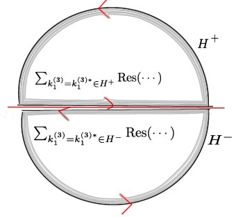
Figure 1: Contour relevant for evaluating (187).

To evaluate this integral, we will make use of the following contour (as shown in the Fig. (1)) integral,

$$\begin{split}\int d\bar{k}_{1}^{(1)}[\cdots]=\oint_{H^{+}}[\cdots]-\oint_{H^{-}}[\cdots]=\frac{i\pi}{2}\sum_{k_{1}^{(3)}=k_{1}^{(3)*}\subset H^{+}}\text{Res}([\cdots])-\sum_{k_{1}^{(3)}=k_{1}^{(3)*}\subset H^{-}}\text{Res}([\cdots])\,.\end{split}$$ (188)

One can see that the integrand has double pole at $k_{1}\cdot v_{1}+i\epsilon=0$. So, we simply close the contour in the opposite and we get zero. However, we see that the impulse corresponding to this diagram has finite non-zero value from (66) which is completely proportional to $v_{i}^{\mu}$. The procedure for recovering the result using Eikonal has been discussed in Kalin:2020fhe .

Appendix C Two master integrals used for the computation of waveform

We analyze the following two integrals,

$$\begin{split}&I^{\mu_{1}\cdots\mu_{n}}_{n}:=\int_{q}\hat{\delta}(q\cdot v_{1}-k\cdot v_{1})\hat{\delta}(q\cdot v_{2})\frac{e^{-iq\cdot b}}{q^{2}}q^{\mu_{1}}\cdots q^{\mu_{n}}\,,\\ &J^{\mu_{1}\cdots\mu_{n}}_{n}:=\int_{q}\hat{\delta}(q\cdot v_{1}-k\cdot v_{1})\hat{\delta}(q\cdot v_{2})\frac{e^{-iq\cdot b}}{q^{2}(k-q)^{2}}q^{\mu_{1}}\cdots q^{\mu_{n}}\,.\end{split}$$ (189)

The two particular cases that we used in the main text are: $J^{\mu}_{1}$ and $J_{0}$. We first start with $J_{0}\,.$

$$\begin{split}J_{(0)}(k)=\int_{q}\hat{\delta}(q\cdot v_{1}-k\cdot v_{1})\hat{\delta}(q\cdot v_{2})\frac{e^{-iq\cdot b}}{q^{2}(k-q)^{2}}\,.\end{split}$$ (190)

We will do this integral by implementing a certain choice of frame,

$$v_{2}^{\mu}=\delta^{\mu}_{0},\,v_{1}^{\mu}=(\gamma,\gamma\beta\,\hat{e}_{v})\,b=(0,|b|\,\hat{e}_{b})\,,$$ (191)

such that, the unit vectors $\hat{e}_{v}$ and $\hat{e}_{b}$ are mutually orthogonal i.e. $\hat{e}_{b}\cdot\hat{e}_{v}=0$. We further proceed with this integral by using the Feynman parametrization method along with the on-shell condition: $k^{2}=0$. Therefore, $J_{0}$ can be written as,

$$\begin{split}J_{(0)}(k)&=\int_{0}^{1}dy\int_{q}\hat{\delta}(q\cdot v_{1}-k\cdot v_{1})\hat{\delta}(q\cdot v_{2})\frac{e^{-iq\cdot b}}{(q-yk)^{4}},\,k^{2}=0\,,\\ &\xrightarrow[]{\bar{q}\rightarrow q-yk}\int_{0}^{1}dye^{-iyk\cdot b}\int_{\bar{q}}\hat{\delta}(\bar{q}\cdot v_{1}-(1-y)k\cdot v_{1})\hat{\delta}(\bar{q}\cdot v_{2}+yk\cdot v_{2})\frac{e^{-i\bar{q}\cdot b}}{\bar{q}^{4}}\,,\\ &=\frac{1}{\gamma}\int_{0}^{1}dy\,e^{-iyk\cdot b}\int_{\bar{q}}\frac{e^{i\tilde{q}\cdot b}}{\Big{[}\tilde{q}^{2}-y^{2}(k\cdot v_{2})^{2}+(\frac{y}{\beta}k\cdot v_{2}+\frac{1-y}{\gamma\beta}k\cdot v_{1})^{2}\Big{]}^{2}}\,,\\ &=\frac{1}{\gamma}\int_{0}^{1}dy\,e^{-iyk\cdot b}\int_{0}^{\infty}dt\,t\int_{\tilde{q}}\exp\Big{[}i\tilde{q}\cdot b-t\tilde{q}^{2}-t\Delta(y)^{2}\Big{]}\,,\\ &=\frac{1}{\gamma}\int_{0}^{1}dy\,e^{-iyk\cdot b}\int_{0}^{\infty}\frac{dt}{4\pi}\,\exp(-\frac{|b|^{2}}{4t}-t\Delta(k,y)^{2})\,,\\ &=\frac{b}{\gamma}\int_{0}^{1}dy\,e^{-iyk\cdot b}\frac{K_{1}\left(|b|{\Delta(k,y)}\right)}{4\pi{\Delta(k,y)}}\end{split}$$ (192)

where,

$$\begin{split}\Delta(k,y)&=\sqrt{-y^{2}(k\cdot v_{2})^{2}+\frac{y^{2}}{\beta^{2}}(k\cdot v_{2})^{2}+\frac{(1-y)^{2}}{\gamma^{2}\beta^{2}}(k\cdot v_{1})^{2}+2\frac{y(1-y)}{\gamma\beta^{2}}(k\cdot v_{2})(k\cdot v_{1})}\,,\\ &=\frac{1}{\sqrt{\gamma^{2}-1}}\sqrt{y^{2}(k\cdot v_{2})^{2}+(1-y)^{2}(k\cdot v_{1})^{2}+2y(1-y)\gamma(k\cdot v_{2})(k\cdot v_{1})}\,.\end{split}$$ (193)

In thee waveform calculation, we have to further perform a integeral over $k$, which in general has the following form,

$$\begin{split}f(x):=\int_{k}e^{-ik\cdot x}T_{\mu_{1}\cdots\mu_{n}}J^{\mu_{1}\cdots\mu_{n}}(k)\,.\end{split}$$ (194)

In the case of $\varphi^{3}$ interaction we have,

$$\begin{split}f(x)&=\int_{k}e^{-ik\cdot x}J_{0}(k),\,k=\Omega n\,,\\ &=\frac{b}{4\pi\gamma}\int_{\Omega}e^{-i\Omega n\cdot x}\int_{0}^{1}dy\,e^{-i\,y\,\Omega(n\cdot b)}\frac{K_{1}[|\Omega|\,|b|\bar{\Delta}(y)]}{|\Omega|\bar{\Delta}(y)}\,\,,\bar{\Delta}(y)\equiv\frac{\Delta(k,y)}{|\Omega|}\,.\end{split}$$ (195)

Now to do the integral over $\Omega$, use the following representation of modified Bessel function:

$$\begin{split}K_{\nu}(x)=\frac{1}{2}(\frac{x}{2})^{\nu}\int_{0}^{\infty}dt\,\exp\Big{(}-t-\frac{x^{2}}{4t}\Big{)}\frac{1}{t^{\nu+1}}\,.\end{split}$$ (196)

Therefore,

$$\begin{split}f(x)&=\frac{|b|}{4\pi\gamma}\int_{0}^{1}dy\,\frac{1}{\bar{\Delta}(y)}\int_{\Omega}e^{-i\Omega n\cdot(x+yb)}\frac{|b|}{4}\bar{\Delta(y)}\int\frac{dt}{t^{2}}\,\exp\Big{(}-t-\frac{\Omega^{2}|b|^{2}\bar{\Delta}(y)^{2}}{4t}\Big{)}\,,\\ &=\frac{|b|^{2}}{16\pi\gamma}\int_{0}^{1}dy\,\int_{0}^{\infty}\frac{dt}{t^{2}}e^{-t}\int d\Omega\,e^{-i\,\Omega\,l}\exp\Big{(}-\frac{\Omega^{2}|b|^{2}\bar{\Delta}(y)^{2}}{4t}\Big{)}\,,\\ &=\frac{|b|^{2}}{16\pi\gamma}\int_{0}^{1}dy\,\int_{0}^{\infty}\frac{dt}{t^{2}}e^{-t}\frac{2\sqrt{\pi}\sqrt{t}e^{-\frac{l^{2}t}{|b|^{2}\bar{\Delta}(y)^{2}}}}{|b|\bar{\Delta}(y)}\,,\\ &=\frac{|b|}{8\sqrt{\pi}\gamma}\int_{0}^{1}dy\frac{1}{\bar{\Delta}(y)}\int_{0}^{\infty}dt\frac{\exp\Big{(}-\frac{l^{2}}{|b|^{2}\bar{\Delta}(y)^{2}}t-t\Big{)}}{t^{3/2}}\,,\\ &=\frac{|b|}{8\sqrt{\pi}\gamma}\int_{0}^{1}dy\frac{1}{\bar{\Delta}(y)}\sqrt{\frac{l^{2}}{|b|^{2}\bar{\Delta}^{2}}+1}\,\,\Gamma(-1/2)\,,\\ &=-\frac{|b|}{4\gamma}\int_{0}^{1}dy\,\frac{1}{\bar{\Delta}(y)}\sqrt{\frac{l^{2}}{|b|^{2}\bar{\Delta}^{2}}+1},\,l:=n\cdot(x+yb)\,.\end{split}$$ (197)

Now come discuss the other important vector integral:

$$\begin{split}J_{(1)}^{\mu}&=\int_{q}\hat{\delta}(q\cdot v_{1}-k\cdot v_{1})\hat{\delta}(q\cdot v_{2})e^{-iq\cdot b}\frac{q^{\mu}}{q^{2}(k-q)^{2}}\,,\\ &=\int_{0}^{1}dy\,e^{-iyk\cdot b}\int_{q}\hat{\delta}(q\cdot v_{1}-(1-y))\hat{\delta}(q\cdot v_{2}+yk\cdot v_{2})\frac{e^{-iq\cdot b}}{q^{4}}(q^{\mu}+yk^{\mu})\,,\\ &:=\mathcal{J}^{\mu}+\frac{|b|\,k^{\mu}}{\gamma}\int_{0}^{1}dy\,y\,\,e^{-iyk\cdot b}\frac{K_{1}(|b|\Delta(k,y))}{4\pi\Delta(k,y)}\,.\end{split}$$ (198)

$\mathcal{J}^{\mu}$ can be solved by reducing the vector integral in scalar integral as follows,

$$\begin{split}\mathcal{J}^{\mu}=\int_{0}^{1}dy\,e^{-iyk\cdot b}\,[\lambda_{b}b^{\mu}+\lambda_{1}v_{1}^{\mu}+\lambda_{2}v_{2}^{\mu}]\,,\end{split}$$ (199)

Now we need to solve the following equations:

• $$\begin{split}\int_{0}^{1}dy\,e^{-iyk\cdot b}\int_{q}\hat{\delta}(q\cdot v_{1}-(1-y))\hat{\delta}(q\cdot v_{2}+yk\cdot v_{2})\frac{e^{-iq\cdot b}}{q^{4}}q\cdot b=\mathcal{J}\cdot b=-\int_{0}^{1}dy\,e^{-iyk\cdot b}b^{2}\lambda_{b}\,.\end{split}$$ (200)

  To do the the $q$ integral of the LHS, we introduce a new parameter $\kappa$ as,

  $$\begin{split}-|b|^{2}\lambda_{b}&=\lim_{\kappa\rightarrow 1}\int_{q}\hat{\delta}(q\cdot v_{1}-(1-y))\hat{\delta}(q\cdot v_{2}+yk\cdot v_{2})\frac{e^{-i\kappa q\cdot b}}{q^{4}}q\cdot b\,,\\ &=i\lim_{\kappa\rightarrow 1}\frac{\partial}{\partial\kappa}\int_{q}\hat{\delta}(q\cdot v_{1}-(1-y))\hat{\delta}(q\cdot v_{2}+yk\cdot v_{2})\frac{e^{-i\kappa q\cdot b}}{q^{4}}\,,\\ &=i\lim_{\kappa\rightarrow 1}\frac{\partial}{\partial\kappa}\hat{J}_{0}(\kappa|b|),\,\hat{J}_{0}(|b|)\equiv\frac{|b|}{\gamma}\frac{K_{1}(|b|\Delta(k,y))}{4\pi\Delta(k,y)}\,.\end{split}$$ (201)

  Hence,

  $$\begin{split}\lambda_{b}=\frac{i\,K_{0}(|b|\Delta(k,y))}{4\pi\gamma}\,.\end{split}$$ (202)

• $$\begin{split}\int_{0}^{1}dy\,e^{-iyk\cdot b}\int_{q}\hat{\delta}(q\cdot v_{1}-(1-y)k\cdot v_{1})\hat{\delta}(q\cdot v_{2}+yk\cdot v_{2})\frac{e^{-iq\cdot b}}{q^{4}}q\cdot v_{1}=\mathcal{J}\cdot v_{1}=\int_{0}^{1}dy\,e^{-iyk\cdot b}[\lambda_{1}+\gamma\lambda_{2}]\,.\end{split}$$ (203)

  Again, the $q$ integral in LHS can be done again by introducing an auxiliary parameter $\kappa$ as,

  $$\begin{split}\lambda_{1}+\gamma\lambda_{2}&=\int_{q}\hat{\delta}(q\cdot v_{1}-(1-y)k\cdot v_{1})\hat{\delta}(q\cdot v_{2}+yk\cdot v_{2})\frac{e^{-iq\cdot b-i\kappa q\cdot v_{1}}}{q^{4}}q\cdot v_{1}\,,\\ &=\int_{q}\hat{\delta}(q\cdot v_{1}-(1-y)k\cdot v_{1})\hat{\delta}(q\cdot v_{2}+yk\cdot v_{2})\frac{e^{-iq\cdot b}}{q^{4}}(1-y)k\cdot v_{1}\,,\\ &=(1-y)k\cdot v_{1}\hat{J}_{0}\,.\end{split}$$ (204)

• $$\begin{split}\int_{0}^{1}dy\,e^{-iyk\cdot b}\int_{q}\hat{\delta}(q\cdot v_{1}-(1-y)k\cdot v_{1})\hat{\delta}(q\cdot v_{2}+yk\cdot v_{2})\frac{e^{-iq\cdot b}}{q^{4}}q\cdot v_{2}=\mathcal{J}\cdot v_{2}=\int_{0}^{1}dy\,e^{-iyk\cdot b}[\gamma\lambda_{1}+\lambda_{2}]\,.\end{split}$$ (205)

  Hence,

  $$\begin{split}\gamma\lambda_{1}+\lambda_{2}&=-\int_{q}\hat{\delta}(q\cdot v_{1}-(1-y)k\cdot v_{1})\hat{\delta}(q\cdot v_{2}+yk\cdot v_{2})\frac{e^{-iq\cdot b}}{q^{4}}y(k\cdot v_{2})\,,\\ &=-yk\cdot v_{2}\hat{J}_{0}\,.\end{split}$$ (206)

  Now solving (204) and (206) we get,

  $$\begin{split}&\lambda_{2}=\frac{y(k\cdot v_{2})+\gamma(1-y)k\cdot v_{1}}{\gamma^{2}-1}\hat{J}_{0}\,,\\ &\lambda_{1}=\frac{-\gamma yk\cdot v_{2}-(1-y)k\cdot v_{1}}{\gamma^{2}-1}\hat{J}_{0}\,.\end{split}$$ (207)

Therefore, the contribution to the waveform takes the following form,

$$\begin{split}f(x)&=T_{\mu}\int_{\Omega}e^{-ik\cdot x}\mathcal{J}^{\mu}\,,\\ &=T_{\mu}\int_{\Omega}e^{-ik\cdot x}\int_{0}^{1}dy\,e^{-iyk\cdot b}[\lambda_{b}b^{\mu}+\lambda_{1}v_{1}^{\mu}+\lambda_{2}v_{2}^{\mu}]\,,\\ &=f_{1}+f_{2}+f_{3}\,,\end{split}$$ (208)

where,

$$\begin{split}f_{1}(x|l)&=\frac{-iT\cdot b}{4\pi\gamma}\int_{\Omega}e^{-i\Omega\,(n\cdot x)}\int_{0}^{1}dy\,K_{0}(|b||\Omega|\bar{\Delta}(y))\,,\\ &=\frac{-iT\cdot b}{4\pi\gamma}\int_{0}^{1}dy\int_{0}^{\infty}\frac{dt}{2t}e^{-t}\int_{\Omega}d\Omega\,e^{-i\Omega l}\exp(-\frac{|b|^{2}\Omega^{2}\bar{\Delta}^{2}}{4t})\,,\\ &=\frac{-iT\cdot b}{4\gamma|b|}\int_{0}^{1}dy\frac{1}{\bar{\Delta}(y)}\sqrt{\frac{|b|^{2}\bar{\Delta}^{2}}{|b|^{2}\bar{\Delta}^{2}+l^{2}}}\,,\end{split}$$ (209)

$$\begin{split}f_{2}(x|l)&=T\cdot v_{1}\,\bar{\lambda}_{1}\int_{\Omega}\Omega\,e^{-i\Omega(n\cdot x)}\int_{0}^{1}dy\,e^{-i\Omega y(n\cdot b)}\frac{b}{\gamma}\frac{K_{1}(b|\Omega|\Delta(k,y))}{4\pi|\Omega|\bar{\Delta}(y)}\,,\\ &=\frac{|b|^{2}\,T\cdot v_{1}\,\bar{\lambda}_{1}}{16\pi\gamma}\int_{0}^{1}dy\int_{0}^{\infty}dt\frac{e^{-t}}{t^{2}}\int_{\Omega}e^{-i\Omega l}\Omega\,\exp\Big{(}-\frac{\Omega^{2}|b|^{2}\bar{\Delta}(y)^{2}}{4t}\Big{)}\,,\\ &=-\frac{i|b|^{2}\,T\cdot v_{1}\,\bar{\lambda}_{1}}{4\gamma}\int_{0}^{1}dy\,\frac{l}{|b|^{3}\bar{\Delta}^{3}}\frac{1}{\sqrt{\frac{l^{2}}{|b|^{2}\Delta^{2}}+1}}\,.\end{split}$$ (210)

and,

$$\begin{split}f_{3}(x|l)=-\frac{i\,T\cdot v_{2}\,\bar{\lambda}_{2}}{4\gamma|b|}\int_{0}^{1}dy\,\frac{l}{\bar{\Delta}^{3}}\frac{1}{\sqrt{\frac{l^{2}}{|b|^{2}\Delta^{2}}+1}}\,,\end{split}$$ (211)

where, $\bar{\lambda}_{i}=\frac{\lambda_{i}}{\Omega}$.

Appendix D Non-contribution of $\lambda_{4}\varphi^{4}$ vertex in waveform

In the main text, we have shown using the method of region Beneke:1997zp that the diagram, due to the self-interaction vertex $\lambda_{4}\varphi^{4}$ does not contribute to the scalar waveform as its contribution is purely divergent and has to be avoided while computing the scalar waveform. Now, we show this vanishing of the contribution of the waveform from the four-point scalar vertex alternatively using the Feynman parametrization. We start with the following integral.

$$\begin{split}&\mathcal{K}\equiv\int_{\Omega}e^{-ik\cdot\tilde{x}}\int_{k_{2}}\frac{\hat{\delta}(k_{2}\cdot v_{2})}{k_{2}^{2}}\int_{\tilde{q}}\frac{\hat{\delta}{(\tilde{q}\cdot v_{1})}\hat{\delta}{[({k}-\tilde{q})\cdot v_{2}]}}{\tilde{q}^{2}[k_{2}-(k-\tilde{q})]^{2}}e^{i\tilde{q}\cdot b}\,,\\ &=\int_{0}^{1}dx\int_{\Omega}e^{-ik\cdot\tilde{x}}\int_{k_{2}}\frac{\hat{\delta}(k_{2}\cdot v_{2})}{k_{2}^{2}}\int_{\tilde{q}}\frac{\hat{\delta}{(\tilde{q}\cdot v_{1})}\hat{\delta}{[({k}-\tilde{q})\cdot v_{2}]}}{(x\tilde{q}^{2}+(1-x)[k_{2}^{2}+\tilde{q}^{2}+2k_{2}\cdot\tilde{q}-2k\cdot\tilde{q}-2k_{2}\cdot k])^{2}}e^{i\tilde{q}\cdot b}\,,\\ &\xrightarrow[q^{\prime}+k=\tilde{q}]{}\int_{0}^{1}dx\int_{\Omega}e^{-ik\cdot\tilde{x}}\int_{k_{2}}\frac{\hat{\delta}(k_{2}\cdot v_{2})}{k_{2}^{2}}\int_{q^{\prime}}\frac{\hat{\delta}{\Big{(}({q^{\prime}+k})\cdot v_{1}\Big{)}}\hat{\delta}{(q^{\prime}\cdot v_{2})}}{[x(q^{\prime}+k)^{2}+(1-x)(k_{2}+q^{\prime})^{2}]^{2}}e^{i(q^{\prime}+k)\cdot b}\,.\\ &\text{ Now replacing $x\rightarrow(1-x)$ we achieve, }\\ &\mathcal{K}=\int_{0}^{1}dx\,e^{ik\cdot\tilde{x}}\int_{q^{\prime},k_{2},\Omega}\frac{\hat{\delta}{(q^{\prime}\cdot v_{1}+k\cdot v_{1})}\hat{\delta}{(q^{\prime}\cdot v_{2})}}{k_{2}^{2}[(q^{\prime}+xk_{2})^{2}+k_{2}^{2}\,x\,(1-x)+2k\cdot q^{\prime}(1-x)]^{2}}e^{i(q^{\prime}+k)\cdot b}\,,\\ &\xrightarrow[q^{\prime}+xk_{2}\rightarrow q^{\prime\prime}]{}\int_{0}^{1}dxe^{-ik\cdot\tilde{x}}\int_{q^{\prime\prime},k_{2},\Omega}\frac{\hat{\delta}(k_{2}\cdot v_{2})}{k_{2}^{2}\{(q^{\prime\prime}+k(1-x))^{2}+Q^{2}\}^{2}}\hat{\delta}\Big{(}(q^{\prime\prime}-xk_{2}+k)\cdot v_{1}\Big{)}\\ &\hskip 213.39566pt\times\hat{\delta}\Big{(}(q-xk_{2})\cdot v_{2}\Big{)}\exp({iq^{\prime\prime}\cdot b-ixk_{2}\cdot b+ik\cdot b})\,,\\ &=\int_{0}^{1}dxe^{-ik\cdot\tilde{x}}\int_{q^{\prime\prime},k_{2},\Omega}\frac{\delta(k_{2}\cdot v_{2})}{k_{2}^{2}\{(q^{\prime\prime}+k(1-x))^{2}+Q^{2}\}^{2}}\hat{\delta}\Big{(}q^{\prime\prime}-xk_{2}+k)\cdot v_{1}\Big{)}\hat{\delta}(q^{\prime\prime}\cdot v_{2})\\ &\hskip 213.39566pt\times\exp({iq^{\prime\prime}\cdot b-ixk_{2}\cdot b+ik\cdot b}),\,\,\,\,\,\,k:=\Omega\hat{n}\,,\\ &=\int_{0}^{1}dx\int_{\vec{k_{2}},\vec{q^{\prime\prime}},\Omega}\frac{1}{k_{2}^{2}\{(q^{\prime\prime}+\Omega\hat{n}(1-x))^{2}+Q^{2}\}^{2}}\hat{\delta}\Big{(}(q^{\prime\prime}-xk_{2}+\Omega\hat{n})\cdot v_{1}\Big{)}\\ &\hskip 184.9429pt\times\exp({iq^{\prime\prime}\cdot b-ixk_{2}\cdot b-i{k}\cdot(\tilde{x}-b)})\,,\\ &\xrightarrow[q^{\prime\prime}+\Omega\hat{n}(1-x)=q^{\prime\prime\prime}]{}\int_{0}^{1}dx\int_{\vec{q^{\prime\prime\prime}},\Omega,\vec{k_{2}}}\frac{1}{\{(q^{\prime\prime\prime})^{2}+\underbrace{Q^{2}}_{x(1-x)(\Omega\hat{n}-k_{2})^{2}}\}^{2}k_{2}^{2}}\hat{\delta}(q^{\prime\prime\prime}-xk_{2}+x\,\Omega\hat{n})\cdot v_{1})\\ &\hskip 184.9429pt\times\exp(i(q^{\prime\prime\prime}-\Omega\hat{n}(1-x))\cdot l)\exp({ixk_{2}\cdot b-i\Omega\hat{n}(\tilde{x}-b)})\,,\\ &=\int_{0}^{1}dx\int_{\vec{q^{\prime\prime\prime}},\vec{k_{2}}}\frac{1}{\{(q^{\prime\prime\prime})^{2}+{x(1-x)(-\frac{(q^{\prime\prime\prime}-xk_{2})\cdot v_{1}}{xn\cdot v_{1}}\hat{n}-k_{2})^{2}}\}^{2}k_{2}^{2}}\exp({iq^{\prime\prime\prime}\cdot l})\exp({ixk_{2}\cdot m})\,.\end{split}$$ (212)

where $\vec{l}:=\vec{b}-\frac{\vec{v_{1}}}{x\hat{n}\cdot v_{1}}\hat{n}\cdot(-\tilde{x}+xb),\vec{m}:=-\vec{b}-\frac{\vec{v_{1}}}{\hat{n}\cdot v_{1}}\hat{n}\cdot(-\tilde{x}+xb)$. This change of variable can be done because as:

$$\int_{a}^{b}f(s)ds=\int_{a}^{b}f(a+b-s)ds.$$

Now to do the integral (212), we use the Schwinger parametrisation. Using that (212) can be written as,

$$={\int_{0}^{1}dx\int_{0}^{\infty}\int_{0}^{\infty}dsdt\,t}\frac{\pi^{3/2}\exp\left(-\frac{\left(\rho^{2}+1\right)\left(\frac{\Delta\rho\text{$l_{1}$}}{\rho^{2}+1}-m_{1}x\right){}^{2}}{4\Delta^{2}t}\right)\exp\left(-\frac{l^{2}+\text{$l_{2}$}^{2}\rho^{2}+\text{$l_{3}$}^{2}\rho^{2}}{4\rho^{2}t+4t}-\frac{x\left(m_{2}^{2}x+m_{3}^{2}x\right)}{4(s+t)}\right)}{\Delta t^{2}(s+t)}\,.$$

$m_{2},m_{3}$ are the second and third components of the $\vec{m}$ and

$$\begin{array}{c}\hfill \mathrm{\Delta }:=(1+\frac{\sqrt{x(1-x)}\gamma \beta }{\widehat{n}\cdot v_1}),\rho :=\frac{\sqrt{x(1-x)}\gamma \beta {\widehat{n}}^1}{(\widehat{n}\cdot v_1)x}.\end{array}$$

To this end, one can easily check that the regularised value of this integral is ${\bf 0}$. Hence, we can ignore the contribution of this diagram in the waveform calculation.

Appendix E Massive integral coming from derivative interaction

The integral of interest is the following,

$$\begin{split}J_{(2)}^{\mu\nu}&=\int_{q}\hat{\delta}(q\cdot v_{1}-k\cdot v_{1})\hat{\delta}(q\cdot v_{2})\frac{q^{\mu}q^{\nu}\,e^{-iq\cdot b}}{(q-k)^{2}(q^{2}-m^{2})}\,,\\ &=\int_{0}^{1}dy\,e^{-iy\,k\cdot b}\int_{q}\hat{\delta}(q\cdot v_{1}-(1-y)k\cdot v_{1})\hat{\delta}(q\cdot v_{2}+yk\cdot v_{2})\frac{e^{-iq\cdot b}}{[q^{2}-(1-2y+y^{2})m^{2}]^{2}}(q^{\mu}+yk^{\mu})(q^{\nu}+yk^{\nu})\,.\end{split}$$ (213)

In (213) the term proportional to $k^{\mu}k^{\nu}$ and $q^{\mu}k^{\nu}$ can be done using the same procedure as discussed in Appendix (C). We will concentrate on the term which is proportional to $q^{\mu}q^{\nu}$ which can be expanded in term of basis vectors.

$$\begin{split}\mathcal{J}_{(2)}^{\mu\nu}(\sim q^{\mu}q^{\nu})=\int_{0}^{1}dy\,e^{-iy\,k\cdot b}[\lambda_{\eta}\eta^{\mu\nu}+\lambda_{bb}b^{\mu}b^{\nu}+\lambda_{1b}b^{(\mu}v_{1}^{\nu)}+\lambda_{2b}b^{(\mu}v_{2}^{\nu)}+\lambda_{11}v_{1}^{\mu}v_{1}^{\nu}+\lambda_{22}v_{2}^{\mu}v_{2}^{\nu}+\lambda_{12}v_{1}^{(\mu}v_{2}^{\nu)}]\,.\end{split}$$ (214)

Now to extract the coefficients in (214) one needs to contract the LHS with the tensor structure of the RHS. The equations we need to solve are the following,

• Contracting with $b^{\mu}b^{\nu}$ gives:

  $$\int_{q}\hat{\delta}(q\cdot v_{1}-(1-y)k\cdot v_{1})\hat{\delta}(q\cdot v_{2}+yk\cdot v_{2})\frac{e^{-iq\cdot b}}{[q^{2}-(1-2y+y^{2})m^{2}]^{2}}(q\cdot b)^{2}=\mathcal{X}_{1}=-\lambda_{\eta}|b|^{2}+\lambda_{bb}|b|^{4}\,.$$ (215)

• Contracting with $b^{(\mu}v_{1}^{\nu)}$ gives:

  $$\begin{split}\int_{q}\hat{\delta}(q\cdot v_{1}-(1-y)k\cdot v_{1})\hat{\delta}(q\cdot v_{2}+yk\cdot v_{2})\frac{e^{-iq\cdot b}}{[q^{2}-(1-2y+y^{2})m^{2}]^{2}}(q\cdot b)(q\cdot v_{1})&=\mathcal{X}_{2}\\ &=-\lambda_{1b}\frac{|b|^{2}}{2}-\lambda_{2b}\frac{\gamma|b|^{2}}{2}\,.\end{split}$$ (216)

• Contracting with $b^{(\mu}v_{2}^{\nu)}$ gives:

  $$\begin{split}\int_{q}\hat{\delta}(q\cdot v_{1}-(1-y)k\cdot v_{1})\hat{\delta}(q\cdot v_{2}+yk\cdot v_{2})\frac{e^{-iq\cdot b}}{[q^{2}-(1-2y+y^{2})m^{2}]^{2}}(q\cdot b)(q\cdot v_{2})&=\mathcal{X}_{3}\\ &=-\frac{|b|^{2}}{2}(\lambda_{2b}+\gamma\lambda_{1b})\,.\end{split}$$ (217)

• Contracting with $v_{1}^{\mu}v_{1}^{\nu}$ gives:

  $$\begin{split}\int_{q}\hat{\delta}(q\cdot v_{1}-(1-y)k\cdot v_{1})\hat{\delta}(q\cdot v_{2}+yk\cdot v_{2})\frac{e^{-iq\cdot b}}{[q^{2}-(1-2y+y^{2})m^{2}]^{2}}(q\cdot v_{1})^{2}&=\mathcal{X}_{4}\\ &=\lambda_{\eta}+\lambda_{11}+\lambda_{22}\gamma^{2}+\lambda_{12}\gamma\,.\end{split}$$ (218)

• Contracting with $v_{2}^{\mu}v_{2}^{\nu}$ gives:

  $$\begin{split}\int_{q}\hat{\delta}(q\cdot v_{1}-(1-y)k\cdot v_{1})\hat{\delta}(q\cdot v_{2}+yk\cdot v_{2})\frac{e^{-iq\cdot b}}{[q^{2}-(1-2y+y^{2})m^{2}]^{2}}(q\cdot v_{2})^{2}&=\mathcal{X}_{5}\\ &=\lambda_{\eta}+\lambda_{22}+\lambda_{11}\gamma^{2}+\lambda_{12}\gamma\,.\end{split}$$ (219)

• Contracting with $v_{1}^{(\mu}v_{2}^{\nu)}$ gives:

  $$\begin{split}\int_{q}\hat{\delta}(q\cdot v_{1}-(1-y)k\cdot v_{1})\hat{\delta}(q\cdot v_{2}+yk\cdot v_{2})\frac{e^{-iq\cdot b}}{[q^{2}-(1-2y+y^{2})m^{2}]^{2}}(q\cdot v_{1})(q\cdot v_{2})&=\mathcal{X}_{6}\\ &=\lambda_{\eta}\gamma+\gamma(\lambda_{11}+\lambda_{22})+\frac{\lambda_{12}}{2}(\gamma^{2}+1)\,.\end{split}$$ (220)

• Contracting with $\eta^{\mu\nu}$ gives:

  $$\begin{split}\int_{q}\hat{\delta}(q\cdot v_{1}-(1-y)k\cdot v_{1})\hat{\delta}(q\cdot v_{2}+yk\cdot v_{2})\frac{e^{-iq\cdot b}}{[q^{2}-(1-2y+y^{2})m^{2}]^{2}}q^{2}&=\mathcal{X}_{7}\\ &=4\lambda_{\eta}-\lambda_{bb}|b|^{2}+\lambda_{11}+\lambda_{22}+\lambda_{12}\gamma\,.\end{split}$$ (221)

Solving (215) to (221) we will get,

$$\begin{split}&\lambda_{\eta}\to\frac{\gamma^{2}\mathcal{X}_{7}-2\gamma\mathcal{X}_{6}+\mathcal{X}_{4}+\mathcal{X}_{5}-\mathcal{X}_{7}}{\gamma^{2}-1}+\frac{\mathcal{X}_{1}}{|b|^{2}},\lambda_{\text{bb}}\to\frac{2\mathcal{X}_{1}}{|b|^{4}}+\frac{\gamma^{2}\mathcal{X}_{7}-2\gamma\mathcal{X}_{6}+\mathcal{X}_{4}+\mathcal{X}_{5}+\mathcal{X}_{7}}{|b|^{2}\left(\gamma^{2}-1\right)},\\ &\lambda_{b}\to-\frac{2\left(\gamma\mathcal{X}_{3}-\mathcal{X}_{2}\right)}{|b|^{2}\left(\gamma^{2}-1\right)},\lambda_{2b}\to-\frac{2\left(\gamma\mathcal{X}_{2}-\mathcal{X}_{3}\right)}{|b|^{2}\left(\gamma^{2}-1\right)},\\ &\lambda_{12}\to\frac{2\left(-|b|^{2}\left(\gamma^{3}\left(-\mathcal{X}_{7}\right)+3\gamma^{2}\mathcal{X}_{6}-2\gamma\mathcal{X}_{4}-2\gamma\mathcal{X}_{5}+\gamma\mathcal{X}_{7}+\mathcal{X}_{6}\right)+\gamma\left(\gamma^{2}-1\right)\mathcal{X}_{1}\right)}{|b|^{2}\left(\gamma^{2}-1\right)^{2}},\\ &\lambda_{11}\to\frac{\frac{\left(\gamma^{2}-1\right)\mathcal{X}_{1}}{|b|^{2}}+\gamma^{2}\mathcal{X}_{7}+\left(\gamma^{2}+1\right)\mathcal{X}_{5}-4\gamma\mathcal{X}_{6}+2\mathcal{X}_{4}-\mathcal{X}_{7}}{\left(\gamma^{2}-1\right)^{2}},\\ &\lambda_{22}\to\frac{\frac{\left(\gamma^{2}-1\right)\mathcal{X}_{1}}{|b|^{2}}+\gamma^{2}\mathcal{X}_{7}+\left(\gamma^{2}+1\right)\mathcal{X}_{4}-4\gamma\mathcal{X}_{6}+2\mathcal{X}_{5}-\mathcal{X}_{7}}{\left(\gamma^{2}-1\right)^{2}}\,.\end{split}$$ (222)

Next, we list down the values of the integrals $\mathcal{X}_{i}^{\prime}s\,.$

$$\begin{split}\mathcal{X}_{1}&=-\lim_{\kappa\to 1}\frac{\partial^{2}}{\partial\kappa^{2}}\int_{q}\hat{\delta}(q\cdot v_{1}-(1-y)k\cdot v_{1})\hat{\delta}(q\cdot v_{2}+yk\cdot v_{2})\frac{e^{-iq\cdot b}}{[q^{2}-(1-2y+y^{2})m^{2}]^{2}}\,,\\ &=-\frac{\kappa|b|}{4\pi\gamma}\lim_{\kappa\to 1}\frac{\partial^{2}}{\partial\kappa^{2}}\frac{K_{1}(\kappa|b|\sqrt{\Delta^{2}+(1-2y+y^{2})m^{2}})}{\sqrt{\Delta^{2}+(1-2y+y^{2})m^{2}}}\,,\\ &=-\frac{|b|}{4\pi\gamma}\Big{[}\frac{[|b|^{2}\left(\Delta^{2}+m^{2}(y-1)^{2}\right)+2]K_{1}\left(|b|\sqrt{m^{2}(y-1)^{2}+\Delta^{2}}\right)}{\sqrt{\Delta^{2}+m^{2}(y-1)^{2}}}-|b|K_{2}\left(|b|\sqrt{m^{2}(y-1)^{2}+\Delta^{2}}\right)\Big{]}\,.\end{split}$$ (223)

$$\begin{split}\mathcal{X}_{2}&=i(1-y)k\cdot v_{1}\lim_{\kappa\to 1}\frac{\partial}{\partial\kappa}\int_{q}\hat{\delta}(q\cdot v_{1}-(1-y)k\cdot v_{1})\hat{\delta}(q\cdot v_{2}+yk\cdot v_{2})\frac{e^{-iq\cdot b}}{[q^{2}-(1-2y+y^{2})m^{2}]^{2}}\,,\\ &=-i(1-y)k\cdot v_{1}\frac{|b|^{2}K_{0}\left(|b|\sqrt{m^{2}(y-1)^{2}+\Delta^{2}}\right)}{4\pi\gamma}\,.\end{split}$$ (224)

$$\begin{split}\mathcal{X}_{3}&=-iy\,k\cdot v_{2}\lim_{\kappa\to 1}\frac{\partial}{\partial\kappa}\int_{q}\hat{\delta}(q\cdot v_{1}-(1-y)k\cdot v_{1})\hat{\delta}(q\cdot v_{2}+yk\cdot v_{2})\frac{e^{-iq\cdot b}}{[q^{2}-(1-2y+y^{2})m^{2}]^{2}}\,,\\ &=iy\,k\cdot v_{2}\frac{|b|^{2}K_{0}\left(|b|\sqrt{m^{2}(y-1)^{2}+\Delta^{2}}\right)}{4\pi\gamma}\,.\end{split}$$ (225)

$$\begin{split}\mathcal{X}_{4}&=(1-y)^{2}(k\cdot v_{1})^{2}\int_{q}\hat{\delta}(q\cdot v_{1}-(1-y)k\cdot v_{1})\hat{\delta}(q\cdot v_{2}+yk\cdot v_{2})\frac{e^{-iq\cdot b}}{[q^{2}-(1-2y+y^{2})m^{2}]^{2}}\,,\\ &=(1-y)^{2}(k\cdot v_{1})^{2}\frac{|b|}{4\pi\gamma}\frac{K_{1}(|b|\sqrt{\Delta^{2}+(1-2y+y^{2})m^{2}})}{\sqrt{\Delta^{2}+(1-2y+y^{2})m^{2}}}\,.\end{split}$$ (226)

$$\begin{split}\mathcal{X}_{5}&=y^{2}(k\cdot v_{2})^{2}\int_{q}\hat{\delta}(q\cdot v_{1}-(1-y)k\cdot v_{1})\hat{\delta}(q\cdot v_{2}+yk\cdot v_{2})\frac{e^{-iq\cdot b}}{[q^{2}-(1-2y+y^{2})m^{2}]^{2}}\,,\\ &=y^{2}(k\cdot v_{2})^{2}\frac{|b|}{4\pi\gamma}\frac{K_{1}(|b|\sqrt{\Delta^{2}+(1-2y+y^{2})m^{2}})}{\sqrt{\Delta^{2}+(1-2y+y^{2})m^{2}}}\,.\end{split}$$ (227)

$$\begin{split}\mathcal{X}_{6}&=-y(1-y)(k\cdot v_{1})(k\cdot v_{2})\int_{q}\hat{\delta}(q\cdot v_{1}-(1-y)k\cdot v_{1})\hat{\delta}(q\cdot v_{2}+yk\cdot v_{2})\frac{e^{-iq\cdot b}}{[q^{2}-(1-2y+y^{2})m^{2}]^{2}}\,,\\ &=-y(1-y)(k\cdot v_{1})(k\cdot v_{2})\frac{|b|}{4\pi\gamma}\frac{K_{1}(|b|\sqrt{\Delta^{2}+(1-2y+y^{2})m^{2}})}{\sqrt{\Delta^{2}+(1-2y+y^{2})m^{2}}}\,.\end{split}$$ (228)

The integral of $\mathcal{X}_{7}$ is little bit involved. One can do this integral in the following way,

$$\begin{split}\mathcal{X}_{7}&=\int_{q}\hat{\delta}(q\cdot v_{1}-(1-y)k\cdot v_{1})\hat{\delta}(q\cdot v_{2}+yk\cdot v_{2})\frac{e^{-iq\cdot b}}{[q^{2}-(1-2y+y^{2})m^{2}]^{2}}\Big{[}q^{2}-(1-y)^{2}m^{2}+(1-y)^{2}m^{2}\Big{]}\,.\end{split}$$ (229)

The integral in (229) has two parts and can be evaluated separately,

$$\begin{split}\mathcal{X}_{7}^{(1)}&\equiv\int_{q}\hat{\delta}(q\cdot v_{1}-(1-y)k\cdot v_{1})\hat{\delta}(q\cdot v_{2}+yk\cdot v_{2})\frac{e^{-iq\cdot b}}{[q^{2}-(1-2y+y^{2})m^{2}]}\,,\\ &=\frac{1}{\gamma}\int_{0}^{\infty}\frac{dt}{4\pi}\,\frac{1}{t}\exp\Big{(}-\frac{|b|^{2}}{4t}-t\Delta^{2}-t(1-y)^{2}m^{2}\Big{)}\,,\\ &=\frac{1}{2\pi\gamma}K_{0}(|b|\sqrt{\Delta^{2}+(1-y)^{2}m^{2}})\,.\end{split}$$ (230)

and the second term takes the form,

$$\begin{split}\mathcal{X}_{7}^{(2)}&=(1-y)^{2}m^{2}\,\int_{q}\hat{\delta}(q\cdot v_{1}-(1-y)k\cdot v_{1})\hat{\delta}(q\cdot v_{2}+yk\cdot v_{2})\frac{e^{-iq\cdot b}}{[q^{2}-(1-2y+y^{2})m^{2}]^{2}}\,,\\ &=(1-y)^{2}m^{2}\frac{|b|}{4\pi\gamma}\frac{K_{1}(|b|\sqrt{\Delta^{2}+(1-2y+y^{2})m^{2}})}{\sqrt{\Delta^{2}+(1-2y+y^{2})m^{2}}}\,.\end{split}$$ (231)

Appendix F Computation of worldline radiation diagram using large velocity approximation

We start with (150) (omitting the overall constant which is irrelevant to explain our point).

$$\begin{split}f_{\varphi}(x)&\propto\int_{\Omega}e^{-ik\cdot(x+b_{1})}\int_{\omega,k_{1}}e^{-ik_{1}\cdot b}\hat{\delta}(k_{1}\cdot v_{2})\hat{\delta}[\Omega\,n(m,\Omega)\cdot v_{1}-\omega]\hat{\delta}(k_{1}\cdot v_{1}-\omega)\frac{\Omega(n\cdot k_{1})}{\omega^{2}(k_{1}^{2}-m^{2})}\,.\end{split}$$ (232)

To do the integration over $\Omega$ in (232) we first find the roots of the equation $f(\Omega):=\Omega\,n(m,\Omega)\cdot v_{1}-\omega=0$, which gives,

$$\begin{split}&\hat{\delta}[\Omega\,n(m,\Omega)\cdot v_{1}-\omega]=\frac{\hat{\delta}(\Omega-\Omega_{1})}{|f^{\prime}(\Omega_{1})|}+\frac{\hat{\delta}(\Omega-\Omega_{2})}{|f^{\prime}(\Omega_{2})|},\,\,\\ &\text{where,}\,\,\Omega_{1}(\omega)=\framebox{$\frac{\tilde{\beta}\sqrt{\left(\tilde{\beta}^{2}-1\right)\gamma^{2}m^{2}+\omega^{2}}+\omega}{\left(1-\tilde{\beta}^{2}\right)\gamma}\text{ if }\gamma m<\omega\lor\frac{\omega}{\gamma}<m<\frac{\omega}{\sqrt{1-\tilde{\beta}^{2}}\gamma}$}\,\,\,\,\text{and,}\\ &\vspace{0.5cm}\hskip 34.14322pt\Omega_{2}(\omega)=\framebox{$\frac{\tilde{\beta}\sqrt{\left(\tilde{\beta}^{2}-1\right)\gamma^{2}m^{2}+\omega^{2}}-\omega}{\left(\tilde{\beta}^{2}-1\right)\gamma}\text{ if }\frac{\omega}{\gamma}<m<\frac{\omega}{\sqrt{1-\tilde{\beta}^{2}}\gamma}\,.$}\end{split}$$ (233)

As the observed frequency can not be negative, only the $\Omega_{1}$ solution is relevant to us. Therefore, the integral in (232) can be written as (with $\tilde{x}=x-b_{1}$),

$$\begin{split}f_{\varphi}(x)&\propto\sum_{a=1}^{2}\int_{k_{1}}e^{-i\Omega_{a}\,n(m,\Omega_{a})\cdot(x-b_{1})}e^{-ik_{1}\cdot b}\hat{\delta}(k_{1}\cdot v_{2})\frac{\Omega_{a}\,n(m,\Omega_{a})\cdot k_{1}}{|f^{\prime}(\Omega_{a})|(k_{1}\cdot v_{1}+i\epsilon)^{2}(k_{1}^{2}-m^{2})}\,.\end{split}$$ (234)

The integral could be significantly simplified by putting a suitable IR cutoff in the $\omega$ and $\Omega$ integral with the limit $\frac{m^{2}}{\Omega^{2}}\ll 1$.The argument in favour of this statement is the following: $\frac{1}{m}$ is order of cosmological scales and $\Omega$ for a compact binary of roughly an hour of orbital period is of the order of $10^{-3}$ Hz(1/m $\sim$ 1 Mpc which makes m $\sim$ $10^{-14}$Hz) . One point has to be noted is that, when we are putting the cutoff on the $\omega$ and $\Omega$ integral, it automatically implies that there should be a cutoff on the integral over $k_{1}$ also (coming from the condition $k_{1}\cdot v_{1}=\omega$). However, one could, in principle, argue that, instead of giving the cutoff on the $k_{1}$ integral, one should put a suitable condition on $|v_{1}|$ such that $k_{1}\cdot v_{1}\gg m$, even if $|k_{1}|\rightarrow 0$. Now the part $\sqrt{(k_{1}\cdot v_{1})^{2}-m^{2}\gamma^{2}(1-\tilde{\beta}^{2})}$ coming from the solutions of $\Omega$ takes the following form in terms the parametrization that we have used here: $\sqrt{\gamma^{2}\beta^{2}k_{1}^{(x)2}-m^{2}\gamma^{2}(1-\tilde{\beta}^{2})}=\gamma\beta\sqrt{k_{1}^{(x)2}-\frac{m^{2}}{\gamma^{2}\beta^{2}}+m^{2}\sin^{2}\theta}$. Now, we assume that we can place our at at particular direction on the celestial sphere as shown in the Fig. (2), such that, $\sin^{2}\theta=\frac{1}{\gamma^{2}\beta^{2}}\,.$ For further simplification, we choose $\gamma\beta\rightarrow\infty$ so that $\sin\theta\rightarrow 0$. Hence, the integration that we have to perform is of the form as shown below,

$$\begin{split}f_{\varphi}(x)\sim\int_{\Omega\in|\Omega|_{\textrm{IR}}\gg m}d\Omega\int_{\omega\in|\omega|_{\textrm{IR}}\gg m}d\omega\int_{k_{1},|k_{1}\cdot v_{1}|\gg m}\cdots\,.\end{split}$$ (235)

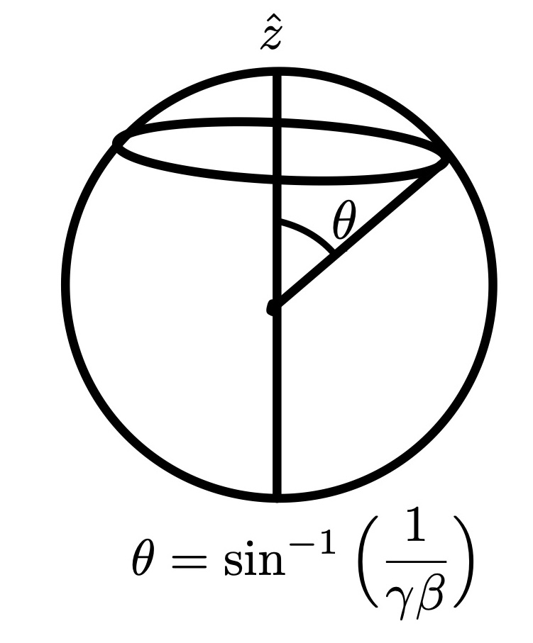
Figure 2: Sketch of the celestial sphere under consideration.

Finally we get,

$$\begin{split}f_{\varphi}(x)\propto\frac{n^{\mu}}{(n\cdot v_{1})^{2}}\underbrace{\int_{k_{1}}e^{-ik_{1}\cdot w_{1}}\hat{\delta}(k_{1}\cdot v_{2})\frac{k_{1\mu}}{(k_{1}\cdot v_{1}+i\epsilon)(k_{1}^{2}-m^{2})}}_{\mathcal{J}_{\mu}^{(2)}},\,\,w_{1}\equiv\frac{n\cdot(x-b_{1})}{n\cdot v_{1}}v_{1}+b\end{split}$$ (236)

where,

$$\begin{split}\mathcal{J}_{\mu}^{(2)}=-\int_{-\infty}^{\infty}d\tau\,\theta(\tau)\frac{(\vec{w}_{1}-\tau\vec{v}_{1})_{i}}{|\vec{w}_{1}-\tau\vec{v}_{1}|^{3}}\,[1+m|\vec{w}_{1}-\tau\vec{v}_{1}|]\,\exp(-m|\vec{w}_{1}-\tau\vec{v}_{1}|)\,.\end{split}$$ (237)

Thenn we proceed as follows:

$$\begin{split}n\cdot\mathcal{J}^{(2)}&\rightarrow-\int d\tau\,\theta(\tau)\frac{n\cdot(\vec{w}_{1}-\tau\vec{v}_{1})}{|\vec{w}_{1}-\tau v_{1}|^{3}}[1+m|\vec{w}_{1}-\tau v_{1}|]\,\exp(-m|\vec{w}_{1}-\tau\vec{v}_{1}|)\,,\\ &=\int_{-\infty}^{\infty}d\tau\,\theta(\tau)\frac{(u_{1}-\tau)\gamma\tilde{\beta}+\chi}{(\gamma^{2}-1)^{3/2}\Big{[}\tau^{2}-u_{1}^{2}-2\tau u_{1}+\frac{b^{2}}{\gamma^{2}-1}\Big{]}^{3/2}}\Bigg{[}1+m(\gamma^{2}-1)^{1/2}\sqrt{\tau^{2}-u_{1}^{2}-2\tau u_{1}+\frac{|b|^{2}}{\gamma^{2}-1}}\Bigg{]}\\ &\hskip 56.9055pt\exp\Big{[}-m(\gamma^{2}-1)^{1/2}\sqrt{\tau^{2}-u_{1}^{2}-2\tau u_{1}+\frac{|b|^{2}}{\gamma^{2}-1}}\Big{]}\,.\end{split}$$ (238)

In the limit of $\sin\theta\rightarrow 0$, the integral has a closed form and smooth massless limit.

gray!10 black

$$\begin{split}\tikzmarkin[disableroundedcorners=false]{x}(0.3,-0.9)(-0.5,1.1)f_{h}\Big{|}_{2}(x)\propto\frac{\gamma}{(n\cdot v_{1})^{2}(\gamma^{2}-1)}\frac{\exp\Big{(}{-m\sqrt{\gamma^{2}-1}\sqrt{\frac{|b|^{2}}{\gamma^{2}-1}-u_{1}^{2}}}\,\Big{)}}{\sqrt{\frac{|b|^{2}}{\gamma^{2}-1}-u_{1}^{2}}}\,.\tikzmarkend{x}\\ \end{split}$$ (239)

References

• (1) LIGO Scientific, VIRGO, NINJA-2 Collaboration, J. Aasi et al., The NINJA-2 project: Detecting and characterizing gravitational waveforms modelled using numerical binary black hole simulations, Class. Quant. Grav. 31 (2014) 115004 [1401.0939].
• (2) LIGO Scientific, Virgo Collaboration, B. P. Abbott et al., Observation of Gravitational Waves from a Binary Black Hole Merger, Phys. Rev. Lett. 116 (2016), no. 6, 061102 [1602.03837].
• (3) LIGO Scientific, Virgo Collaboration, B. P. Abbott et al., GW151226: Observation of Gravitational Waves from a 22-Solar-Mass Binary Black Hole Coalescence, Phys. Rev. Lett. 116 (2016), no. 24, 241103 [1606.04855].
• (4) LIGO Scientific, Virgo Collaboration, B. P. Abbott et al., Properties of the Binary Black Hole Merger GW150914, Phys. Rev. Lett. 116 (2016), no. 24, 241102 [1602.03840].
• (5) LIGO Scientific, VIRGO Collaboration, B. P. Abbott et al., GW170104: Observation of a 50-Solar-Mass Binary Black Hole Coalescence at Redshift 0.2, Phys. Rev. Lett. 118 (2017), no. 22, 221101 [1706.01812], [Erratum: Phys.Rev.Lett. 121, 129901 (2018)].
• (6) LIGO Scientific, Virgo Collaboration, B. P. Abbott et al., A guide to LIGO–Virgo detector noise and extraction of transient gravitational-wave signals, Class. Quant. Grav. 37 (2020), no. 5, 055002 [1908.11170].
• (7) M. Pürrer and C.-J. Haster, Gravitational waveform accuracy requirements for future ground-based detectors, Phys. Rev. Res. 2 (2020), no. 2, 023151 [1912.10055].
• (8) K. S. Stelle, Classical gravity with higher derivatives, General Relativity and Gravitation 9 (1978), no. 4, 353–371.
• (9) S. O. Alexeev and M. V. Pomazanov, Black hole solutions with dilatonic hair in higher curvature gravity, Phys. Rev. D 55 (1997) 2110–2118 [hep-th/9605106].
• (10) A. Lehébel, Compact astrophysical objects in modified gravity. PhD thesis, Orsay, 2018. 1810.04434.
• (11) M. S. Volkov, Hairy black holes in the XX-th and XXI-st centuries, in 14th Marcel Grossmann Meeting on Recent Developments in Theoretical and Experimental General Relativity, Astrophysics, and Relativistic Field Theories, vol. 2, pp. 1779–1798. 2017. 1601.08230.
• (12) M. Kunz and D. Sapone, Dark Energy versus Modified Gravity, Phys. Rev. Lett. 98 (2007) 121301 [astro-ph/0612452].
• (13) T. Damour and G. Esposito-Farese, Tensor multiscalar theories of gravitation, Class. Quant. Grav. 9 (1992) 2093–2176.
• (14) M. Horbatsch, H. O. Silva, D. Gerosa, P. Pani, E. Berti, L. Gualtieri and U. Sperhake, Tensor-multi-scalar theories: relativistic stars and 3 + 1 decomposition, Class. Quant. Grav. 32 (2015), no. 20, 204001 [1505.07462].
• (15) O. Schön and D. D. Doneva, Tensor-multiscalar gravity: Equations of motion to 2.5 post-Newtonian order, Phys. Rev. D 105 (2022), no. 6, 064034 [2112.07388].
• (16) M. Rainer and A. Zhuk, Tensor - multi - scalar theories from multidimensional cosmology, Phys. Rev. D 54 (1996) 6186–6192 [gr-qc/9608020].
• (17) A. De Felice and S. Tsujikawa, Conditions for the cosmological viability of the most general scalar-tensor theories and their applications to extended Galileon dark energy models, JCAP 02 (2012) 007 [1110.3878].
• (18) R. Gsponer and J. Noller, Tachyonic stability priors for dark energy, Phys. Rev. D 105 (2022), no. 6, 064002 [2107.01044].
• (19) H. Weyl, Space, Time, Matter. Dover, USA, 1922.
• (20) L. Blanchet, Gravitational Radiation from Post-Newtonian Sources and Inspiralling Compact Binaries, Living Rev. Rel. 17 (2014) 2 [1310.1528].
• (21) G. Schäfer and P. Jaranowski, Hamiltonian formulation of general relativity and post-Newtonian dynamics of compact binaries, Living Rev. Rel. 21 (2018), no. 1, 7 [1805.07240].
• (22) T. Futamase and Y. Itoh, The Post-Newtonian Approximation for Relativistic Compact Binaries, Living Reviews in Relativity 10 (2007), no. 1, 2.
• (23) M. E. Pati and C. M. Will, PostNewtonian gravitational radiation and equations of motion via direct integration of the relaxed Einstein equations. 1. Foundations, Phys. Rev. D 62 (2000) 124015 [gr-qc/0007087].
• (24) H. Tagoshi, A. Ohashi and B. J. Owen, Gravitational field and equations of motion of spinning compact binaries to 2.5 postNewtonian order, Phys. Rev. D 63 (2001) 044006 [gr-qc/0010014].
• (25) G. Faye, L. Blanchet and A. Buonanno, Higher-order spin effects in the dynamics of compact binaries. I. Equations of motion, Phys. Rev. D 74 (2006) 104033 [gr-qc/0605139].
• (26) L. Blanchet, A. Buonanno and G. Faye, Higher-order spin effects in the dynamics of compact binaries. II. Radiation field, Phys. Rev. D 74 (2006) 104034 [gr-qc/0605140], [Erratum: Phys.Rev.D 75, 049903 (2007), Erratum: Phys.Rev.D 81, 089901 (2010)].
• (27) L. Blanchet, T. Damour, G. Esposito-Farese and B. R. Iyer, Gravitational radiation from inspiralling compact binaries completed at the third post-Newtonian order, Phys. Rev. Lett. 93 (2004) 091101 [gr-qc/0406012].
• (28) T. Damour, P. Jaranowski and G. Schaefer, Equivalence between the ADM-Hamiltonian and the harmonic coordinates approaches to the third postNewtonian dynamics of compact binaries, Phys. Rev. D 63 (2001) 044021 [gr-qc/0010040], [Erratum: Phys.Rev.D 66, 029901 (2002)].
• (29) Y. Itoh and T. Futamase, New derivation of a third postNewtonian equation of motion for relativistic compact binaries without ambiguity, Phys. Rev. D 68 (2003) 121501 [gr-qc/0310028].
• (30) Y. Boetzel, C. K. Mishra, G. Faye, A. Gopakumar and B. R. Iyer, Gravitational-wave amplitudes for compact binaries in eccentric orbits at the third post-Newtonian order: Tail contributions and postadiabatic corrections, Phys. Rev. D 100 (2019), no. 4, 044018 [1904.11814].
• (31) C. K. Mishra, K. G. Arun and B. R. Iyer, 2.5PN kick from black-hole binaries in circular orbit: Nonspinning case, Springer Proc. Phys. 157 (2014) 169–175 [1304.5915].
• (32) S. Kumar, A. Chowdhuri and A. Bhattacharyya, Prospects of detecting deviations to Kerr geometry with radiation reaction effects in EMRIs, 2311.05983.
• (33) R. Fujita and B. R. Iyer, Spherical harmonic modes of 5.5 post-Newtonian gravitational wave polarisations and associated factorised resummed waveforms for a particle in circular orbit around a Schwarzschild black hole, Phys. Rev. D 82 (2010) 044051 [1005.2266].
• (34) G. Faye, L. Blanchet and B. R. Iyer, Non-linear multipole interactions and gravitational-wave octupole modes for inspiralling compact binaries to third-and-a-half post-Newtonian order, Class. Quant. Grav. 32 (2015), no. 4, 045016 [1409.3546].
• (35) L. Blanchet, G. Faye, Q. Henry, F. Larrouturou and D. Trestini, Gravitational Wave Flux and Quadrupole Modes from Quasi-Circular Non-Spinning Compact Binaries to the Fourth Post-Newtonian Order, 2304.11186.
• (36) B. M. Barker and R. F. O’Connell, Gravitational two-body problem with arbitrary masses, spins, and quadrupole moments, Phys. Rev. D 12 (Jul, 1975) 329–335.
• (37) L. E. Kidder, C. M. Will and A. G. Wiseman, Spin effects in the inspiral of coalescing compact binaries, Phys. Rev. D 47 (1993), no. 10, R4183–R4187 [gr-qc/9211025].
• (38) G. Cho, R. A. Porto and Z. Yang, Gravitational radiation from inspiralling compact objects: Spin effects to the fourth post-Newtonian order, Phys. Rev. D 106 (2022), no. 10, L101501 [2201.05138].
• (39) J. Steinhoff, S. Hergt and G. Schaefer, On the next-to-leading order gravitational spin(1)-spin(2) dynamics, Phys. Rev. D 77 (2008) 081501 [0712.1716].
• (40) X. Zhang, T. Liu and W. Zhao, Gravitational radiation from compact binary systems in screened modified gravity, Phys. Rev. D 95 (2017), no. 10, 104027 [1702.08752].
• (41) L. Bernard, L. Blanchet and D. Trestini, Gravitational waves in scalar-tensor theory to one-and-a-half post-Newtonian order, JCAP 08 (2022), no. 08, 008 [2201.10924].
• (42) A. Chowdhuri and A. Bhattacharyya, Study of eccentric binaries in Horndeski gravity, Phys. Rev. D 106 (2022), no. 6, 064046 [2203.09917].
• (43) X. Zhang, W. Zhao, T. Liu, K. Lin, C. Zhang, X. Zhao, S. Zhang, T. Zhu and A. Wang, Angular momentum loss for eccentric compact binary in screened modified gravity, JCAP 01 (2019) 019 [1811.00339].
• (44) A. Saffer and N. Yunes, Angular momentum loss for a binary system in Einstein-Æther theory, Phys. Rev. D 98 (2018), no. 12, 124015 [1807.08049].
• (45) K. Lin, X. Zhao, C. Zhang, T. Liu, B. Wang, S. Zhang, X. Zhang, W. Zhao, T. Zhu and A. Wang, Gravitational waveforms, polarizations, response functions, and energy losses of triple systems in Einstein-aether theory, Phys. Rev. D 99 (2019), no. 2, 023010 [1810.07707].
• (46) Z. Li, J. Qiao, T. Liu, T. Zhu and W. Zhao, Gravitational waveform and polarization from binary black hole inspiral in dynamical Chern-Simons gravity: from generation to propagation, JCAP 04 (2023) 006 [2211.12188].
• (47) B. Shiralilou, T. Hinderer, S. M. Nissanke, N. Ortiz and H. Witek, Post-Newtonian gravitational and scalar waves in scalar-Gauss–Bonnet gravity, Class. Quant. Grav. 39 (2022), no. 3, 035002 [2105.13972].
• (48) W. D. Goldberger and I. Z. Rothstein, An Effective field theory of gravity for extended objects, Phys. Rev. D 73 (2006) 104029 [hep-th/0409156].
• (49) W. D. Goldberger and A. Ross, Gravitational radiative corrections from effective field theory, Phys. Rev. D 81 (2010) 124015 [0912.4254].
• (50) B. Kol and M. Smolkin, Non-Relativistic Gravitation: From Newton to Einstein and Back, Class. Quant. Grav. 25 (2008) 145011 [0712.4116].
• (51) W. D. Goldberger, Les Houches lectures on effective field theories and gravitational radiation, in Les Houches Summer School - Session 86: Particle Physics and Cosmology: The Fabric of Spacetime. 1, 2007. hep-ph/0701129.
• (52) R. A. Porto, The effective field theorist’s approach to gravitational dynamics, Phys. Rept. 633 (2016) 1–104 [1601.04914].
• (53) S. Foffa and R. Sturani, Effective field theory methods to model compact binaries, Class. Quant. Grav. 31 (2014), no. 4, 043001 [1309.3474].
• (54) I. Z. Rothstein, Progress in effective field theory approach to the binary inspiral problem, General Relativity and Gravitation 46 (2014), no. 6, 1726.
• (55) M. Levi, Effective Field Theories of Post-Newtonian Gravity: A comprehensive review, Rept. Prog. Phys. 83 (2020), no. 7, 075901 [1807.01699].
• (56) A. Bhattacharyya, S. Ghosh and S. Pal, Worldline effective field theory of inspiralling black hole binaries in presence of dark photon and axionic dark matter, JHEP 08 (2023) 207 [2305.15473].
• (57) R. F. Diedrichs, D. Schmitt and L. Sagunski, Binary Systems in Massive Scalar-Tensor Theories: Next-to-Leading Order Gravitational Waveform from Effective Field Theory, 2311.04274.
• (58) J. Huang, M. C. Johnson, L. Sagunski, M. Sakellariadou and J. Zhang, Prospects for axion searches with Advanced LIGO through binary mergers, Phys. Rev. D 99 (2019), no. 6, 063013 [1807.02133].
• (59) L. Bernard, E. Dones and S. Mougiakakos, Tidal effects up to next-to-next-to leading post-Newtonian order in massless scalar-tensor theories, 2310.19679.
• (60) W. Junker and G. Schäfer, Binary systems: higher order gravitational radiation damping and wave emission, Monthly Notices of the Royal Astronomical Society 254 (1992) 146–164.
• (61) T. Damour and N. Deruelle, General relativistic celestial mechanics of binary systems. II. The post-newtonian timing formula, Annales De L Institut Henri Poincare-physique Theorique 44 (1986) 263–292.
• (62) L. De Vittori, P. Jetzer and A. Klein, Gravitational wave energy spectrum of hyperbolic encounters, Phys. Rev. D 86 (2012) 044017 [1207.5359].
• (63) J. García-Bellido and S. Nesseris, Gravitational wave energy emission and detection rates of Primordial Black Hole hyperbolic encounters, Phys. Dark Univ. 21 (2018) 61–69 [1711.09702].
• (64) M. Gröbner, P. Jetzer, M. Haney, S. Tiwari and W. Ishibashi, A note on the gravitational wave energy spectrum of parabolic and hyperbolic encounters, Class. Quant. Grav. 37 (2020), no. 6, 067002 [2001.05187].
• (65) S. Capozziello, M. De Laurentis, F. De Paolis, G. Ingrosso and A. Nucita, Gravitational waves from hyperbolic encounters, Mod. Phys. Lett. A 23 (2008) 99–107 [0801.0122].
• (66) J. Majar and M. Vasuth, Gravitational waveforms for spinning compact binaries, Phys. Rev. D 77 (2008) 104005 [0806.2273].
• (67) J. Majar, P. Forgacs and M. Vasuth, Gravitational waves from binaries on unbound orbits, Phys. Rev. D 82 (2010) 064041 [1009.5042].
• (68) L. De Vittori, A. Gopakumar, A. Gupta and P. Jetzer, Gravitational waves from spinning compact binaries in hyperbolic orbits, Phys. Rev. D 90 (2014), no. 12, 124066 [1410.6311].
• (69) G. Cho, A. Gopakumar, M. Haney and H. M. Lee, Gravitational waves from compact binaries in post-Newtonian accurate hyperbolic orbits, Phys. Rev. D 98 (2018), no. 2, 024039 [1807.02380].
• (70) L. J. Rubbo, K. Holley-Bockelmann and L. S. Finn, Event rate for extreme mass ratio burst signals in the lisa band, AIP Conf. Proc. 873 (2006), no. 1, 284–288 [astro-ph/0602445].
• (71) C. P. L. Berry and J. R. Gair, Observing the Galaxy’s massive black hole with gravitational wave bursts, Mon. Not. Roy. Astron. Soc. 429 (2013) 589–612 [1210.2778].
• (72) C. P. L. Berry and J. R. Gair, Extreme-mass-ratio-bursts from extragalactic sources, Mon. Not. Roy. Astron. Soc. 433 (2013) 3572–3583 [1306.0774].
• (73) C. P. L. Berry and J. R. Gair, Expectations for extreme-mass-ratio bursts from the Galactic Centre, Mon. Not. Roy. Astron. Soc. 435 (2013) 3521–3540 [1307.7276].
• (74) A. Chowdhuri, R. K. Singh, K. Kangsabanik and A. Bhattacharyya, Gravitational radiation from hyperbolic encounters in the presence of dark matter, 2306.11787.
• (75) M. Caldarola, S. Kuroyanagi, S. Nesseris and J. Garcia-Bellido, The effects of orbital precession on hyperbolic encounters, 2307.00915.
• (76) T. Damour, Gravitational scattering, post-Minkowskian approximation and Effective One-Body theory, Phys. Rev. D 94 (2016), no. 10, 104015 [1609.00354].
• (77) D. Bini and T. Damour, Gravitational scattering of two black holes at the fourth post-Newtonian approximation, Phys. Rev. D 96 (2017), no. 6, 064021 [1706.06877].
• (78) D. Bini and T. Damour, Gravitational spin-orbit coupling in binary systems, post-Minkowskian approximation and effective one-body theory, Phys. Rev. D 96 (2017), no. 10, 104038 [1709.00590].
• (79) T. Damour, High-energy gravitational scattering and the general relativistic two-body problem, Phys. Rev. D 97 (2018), no. 4, 044038 [1710.10599].
• (80) T. Damour, Classical and quantum scattering in post-Minkowskian gravity, Phys. Rev. D 102 (2020), no. 2, 024060 [1912.02139].
• (81) D. Bini, T. Damour and A. Geralico, Scattering of tidally interacting bodies in post-Minkowskian gravity, Phys. Rev. D 101 (2020), no. 4, 044039 [2001.00352].
• (82) D. Bini, T. Damour, A. Geralico, S. Laporta and P. Mastrolia, Gravitational dynamics at $O(G^{6})$: perturbative gravitational scattering meets experimental mathematics, 2008.09389.
• (83) T. Damour, Radiative contribution to classical gravitational scattering at the third order in $G$, Phys. Rev. D 102 (2020), no. 12, 124008 [2010.01641].
• (84) D. Bini, T. Damour, A. Geralico, S. Laporta and P. Mastrolia, Gravitational scattering at the seventh order in $G$: nonlocal contribution at the sixth post-Newtonian accuracy, Phys. Rev. D 103 (2021), no. 4, 044038 [2012.12918].
• (85) D. Bini, T. Damour and A. Geralico, Radiative contributions to gravitational scattering, Phys. Rev. D 104 (2021), no. 8, 084031 [2107.08896].
• (86) D. Bini, T. Damour and A. Geralico, Radiated momentum and radiation reaction in gravitational two-body scattering including time-asymmetric effects, Phys. Rev. D 107 (2023), no. 2, 024012 [2210.07165].
• (87) T. Damour and P. Rettegno, Strong-field scattering of two black holes: Numerical relativity meets post-Minkowskian gravity, Phys. Rev. D 107 (2023), no. 6, 064051 [2211.01399].
• (88) D. Bini and T. Damour, Radiation-reaction and angular momentum loss at the second post-Minkowskian order, Phys. Rev. D 106 (2022), no. 12, 124049 [2211.06340].
• (89) P. Rettegno, G. Pratten, L. M. Thomas, P. Schmidt and T. Damour, Strong-field scattering of two spinning black holes: Numerical relativity versus post-Minkowskian gravity, Phys. Rev. D 108 (2023), no. 12, 124016 [2307.06999].
• (90) D. Bini, T. Damour and A. Geralico, Comparing one-loop gravitational bremsstrahlung amplitudes to the multipolar-post-Minkowskian waveform, Phys. Rev. D 108 (2023), no. 12, 124052 [2309.14925].
• (91) A. Ceresole, T. Damour, A. Nagar and P. Rettegno, Double copy, Kerr-Schild gauges and the Effective-One-Body formalism, 2312.01478.
• (92) G. Kälin and R. A. Porto, Post-Minkowskian Effective Field Theory for Conservative Binary Dynamics, JHEP 11 (2020) 106 [2006.01184].
• (93) C. Cheung and M. P. Solon, Tidal Effects in the Post-Minkowskian Expansion, Phys. Rev. Lett. 125 (2020), no. 19, 191601 [2006.06665].
• (94) G. Kälin, Z. Liu and R. A. Porto, Conservative Tidal Effects in Compact Binary Systems to Next-to-Leading Post-Minkowskian Order, Phys. Rev. D 102 (2020) 124025 [2008.06047].
• (95) K. Haddad and A. Helset, Tidal effects in quantum field theory, JHEP 12 (2020) 024 [2008.04920].
• (96) G. Kälin, Z. Liu and R. A. Porto, Conservative Dynamics of Binary Systems to Third Post-Minkowskian Order from the Effective Field Theory Approach, Phys. Rev. Lett. 125 (2020), no. 26, 261103 [2007.04977].
• (97) C. Dlapa, G. Kälin, Z. Liu and R. A. Porto, Dynamics of binary systems to fourth Post-Minkowskian order from the effective field theory approach, Phys. Lett. B 831 (2022) 137203 [2106.08276].
• (98) C. Dlapa, G. Kälin, Z. Liu and R. A. Porto, Conservative Dynamics of Binary Systems at Fourth Post-Minkowskian Order in the Large-Eccentricity Expansion, Phys. Rev. Lett. 128 (2022), no. 16, 161104 [2112.11296].
• (99) G. Kälin, J. Neef and R. A. Porto, Radiation-reaction in the Effective Field Theory approach to Post-Minkowskian dynamics, JHEP 01 (2023) 140 [2207.00580].
• (100) R. Jinno, G. Kälin, Z. Liu and H. Rubira, Machine learning Post-Minkowskian integrals, JHEP 07 (2023) 181 [2209.01091].
• (101) C. Dlapa, G. Kälin, Z. Liu, J. Neef and R. A. Porto, Radiation Reaction and Gravitational Waves at Fourth Post-Minkowskian Order, Phys. Rev. Lett. 130 (2023), no. 10, 101401 [2210.05541].
• (102) C. Dlapa, G. Kälin, Z. Liu and R. A. Porto, Bootstrapping the relativistic two-body problem, 2304.01275.
• (103) M. J. Duff, Quantum Tree Graphs and the Schwarzschild Solution, Phys. Rev. D 7 (Apr, 1973) 2317–2326.
• (104) B. R. Holstein and J. F. Donoghue, Classical physics and quantum loops, Phys. Rev. Lett. 93 (2004) 201602 [hep-th/0405239].
• (105) D. Neill and I. Z. Rothstein, Classical Space-Times from the S Matrix, Nucl. Phys. B 877 (2013) 177–189 [1304.7263].
• (106) N. E. J. Bjerrum-Bohr, J. F. Donoghue and P. Vanhove, On-shell Techniques and Universal Results in Quantum Gravity, JHEP 02 (2014) 111 [1309.0804].
• (107) A. Luna, I. Nicholson, D. O’Connell and C. D. White, Inelastic Black Hole Scattering from Charged Scalar Amplitudes, JHEP 03 (2018) 044 [1711.03901].
• (108) N. E. J. Bjerrum-Bohr, P. H. Damgaard, G. Festuccia, L. Planté and P. Vanhove, General Relativity from Scattering Amplitudes, Phys. Rev. Lett. 121 (2018), no. 17, 171601 [1806.04920].
• (109) D. A. Kosower, B. Maybee and D. O’Connell, Amplitudes, Observables, and Classical Scattering, JHEP 02 (2019) 137 [1811.10950].
• (110) A. Buonanno, M. Khalil, D. O’Connell, R. Roiban, M. P. Solon and M. Zeng, Snowmass White Paper: Gravitational Waves and Scattering Amplitudes, in Snowmass 2021. 4, 2022. 2204.05194.
• (111) C. Cheung, I. Z. Rothstein and M. P. Solon, From Scattering Amplitudes to Classical Potentials in the Post-Minkowskian Expansion, Phys. Rev. Lett. 121 (2018), no. 25, 251101 [1808.02489].
• (112) A. Cristofoli, N. E. J. Bjerrum-Bohr, P. H. Damgaard and P. Vanhove, Post-Minkowskian Hamiltonians in general relativity, Phys. Rev. D 100 (2019), no. 8, 084040 [1906.01579].
• (113) C. Cheung and M. P. Solon, Classical gravitational scattering at $\mathcal{O}$(G3) from Feynman diagrams, JHEP 06 (2020) 144 [2003.08351].
• (114) Z. Bern, C. Cheung, R. Roiban, C.-H. Shen, M. P. Solon and M. Zeng, Scattering Amplitudes and the Conservative Hamiltonian for Binary Systems at Third Post-Minkowskian Order, Phys. Rev. Lett. 122 (2019), no. 20, 201603 [1901.04424].
• (115) Z. Bern, C. Cheung, R. Roiban, C.-H. Shen, M. P. Solon and M. Zeng, Black Hole Binary Dynamics from the Double Copy and Effective Theory, JHEP 10 (2019) 206 [1908.01493].
• (116) A. Laddha and A. Sen, Logarithmic Terms in the Soft Expansion in Four Dimensions, JHEP 10 (2018) 056 [1804.09193].
• (117) A. Laddha and A. Sen, Gravity Waves from Soft Theorem in General Dimensions, JHEP 09 (2018) 105 [1801.07719].
• (118) A. Laddha and A. Sen, Observational Signature of the Logarithmic Terms in the Soft Graviton Theorem, Phys. Rev. D 100 (2019), no. 2, 024009 [1806.01872].
• (119) A. Laddha and A. Sen, Classical proof of the classical soft graviton theorem in D$>$4, Phys. Rev. D 101 (2020), no. 8, 084011 [1906.08288].
• (120) A. Manu, D. Ghosh, A. Laddha and P. V. Athira, Soft radiation from scattering amplitudes revisited, JHEP 05 (2021) 056 [2007.02077].
• (121) D. Ghosh and B. Sahoo, Spin-dependent gravitational tail memory in $D=4$, Phys. Rev. D 105 (2022), no. 2, 025024 [2106.10741].
• (122) M. A. and D. Ghosh, Classical spinning soft factors from gauge theory amplitudes, 2210.07561.
• (123) G. Mogull, J. Plefka and J. Steinhoff, Classical black hole scattering from a worldline quantum field theory, JHEP 02 (2021) 048 [2010.02865].
• (124) G. U. Jakobsen, G. Mogull, J. Plefka and J. Steinhoff, Classical Gravitational Bremsstrahlung from a Worldline Quantum Field Theory, Phys. Rev. Lett. 126 (2021), no. 20, 201103 [2101.12688].
• (125) G. U. Jakobsen, G. Mogull, J. Plefka and J. Steinhoff, Gravitational Bremsstrahlung and Hidden Supersymmetry of Spinning Bodies, Phys. Rev. Lett. 128 (2022), no. 1, 011101 [2106.10256].
• (126) G. U. Jakobsen, G. Mogull, J. Plefka and J. Steinhoff, SUSY in the sky with gravitons, JHEP 01 (2022) 027 [2109.04465].
• (127) G. U. Jakobsen, G. Mogull, J. Plefka, B. Sauer and Y. Xu, Conservative Scattering of Spinning Black Holes at Fourth Post-Minkowskian Order, Phys. Rev. Lett. 131 (2023), no. 15, 151401 [2306.01714].
• (128) G. U. Jakobsen, G. Mogull, J. Plefka and B. Sauer, Dissipative Scattering of Spinning Black Holes at Fourth Post-Minkowskian Order, Phys. Rev. Lett. 131 (2023), no. 24, 241402 [2308.11514].
• (129) G. U. Jakobsen, G. Mogull, J. Plefka and B. Sauer, Tidal effects and renormalization at fourth post-Minkowskian order, 2312.00719.
• (130) F. Bastianelli, F. Comberiati and L. de la Cruz, Light bending from eikonal in worldline quantum field theory, JHEP 02 (2022) 209 [2112.05013].
• (131) F. Diaz-Jaramillo, O. Hohm and J. Plefka, Double field theory as the double copy of Yang-Mills theory, Phys. Rev. D 105 (2022), no. 4, 045012 [2109.01153].
• (132) F. Comberiati and C. Shi, Classical Double Copy of Spinning Worldline Quantum Field Theory, JHEP 04 (2023) 008 [2212.13855].
• (133) A. Buonanno and T. Damour, Effective one-body approach to general relativistic two-body dynamics, Phys. Rev. D 59 (1999) 084006 [gr-qc/9811091].
• (134) M. J. Strassler, Field theory without Feynman diagrams: One loop effective actions, Nucl. Phys. B 385 (1992) 145–184 [hep-ph/9205205].
• (135) X. Feal, A. Tarasov and R. Venugopalan, QED as a many-body theory of worldlines: General formalism and infrared structure, Phys. Rev. D 106 (2022), no. 5, 056009 [2206.04188].
• (136) N. Ahmadiniaz, J. P. Edwards, C. Lopez-Arcos, M. A. Lopez-Lopez, C. M. Mata, J. Nicasio and C. Schubert, Summing Feynman diagrams in the worldline formalism, PoS LL2022 (2022) 052 [2208.06585].
• (137) D. M. Eardley, Observable effects of a scalar gravitational field in a binary pulsar, Astrophys. J. Lett. 196 (Mar., 1975) L59–L62.
• (138) D. Amati, M. Ciafaloni and G. Veneziano, Higher Order Gravitational Deflection and Soft Bremsstrahlung in Planckian Energy Superstring Collisions, Nucl. Phys. B 347 (1990) 550–580.
• (139) M. Beneke and V. A. Smirnov, Asymptotic expansion of Feynman integrals near threshold, Nucl. Phys. B 522 (1998) 321–344 [hep-ph/9711391].
• (140) D. Amati, M. Ciafaloni and G. Veneziano, Superstring Collisions at Planckian Energies, Phys. Lett. B 197 (1987) 81.
• (141) Z. Bern, A. Luna, R. Roiban, C.-H. Shen and M. Zeng, Spinning black hole binary dynamics, scattering amplitudes, and effective field theory, Phys. Rev. D 104 (2021), no. 6, 065014 [2005.03071].
• (142) B. Maybee, D. O’Connell and J. Vines, Observables and amplitudes for spinning particles and black holes, JHEP 12 (2019) 156 [1906.09260].