Autonomous system analysis of the late-time cosmological solutions and their stability in higher-order symmetric teleparallel equivalent of general relativity

Abstract

Cosmological dynamics are investigated in detail through systematic procedures by using the autonomous system analyses of gravitational field equations in higher-order symmetric teleparallel equivalent of general relativity. The explicit analyses of the late-time cosmic evolutions are demonstrated for fundamental three types of models under the presence of non-relativistic matter (i.e., dark matter and baryons) as well as radiation. The stability of cosmological solutions is also explored by examining non-hyperbolic critical points based on the center manifold theory. It is shown that the acceleration of the universe can be achieved with the higher curvature gravity. Three different models were considered for the study and dynamical systems analysis technique is incorporated. The main finding of the present analyses is that cosmological solutions in higher-order symmetric teleparallel equivalent of general relativity can effectively fit observable datasets. This is depicted by phase space portraits and qualitative evolution of the cosmological models.

I Introduction

The most significant challenge that theoretical physicist have encountered is the universe’s late-time accelerated expansion. Many observational indicators, including type Ia supernovae (SNIa)[1, 2, 3], Large Scale Structure (LSS), the Cosmic Microwave Background (CMB), and Baryonic Acoustic Oscillations (BAO) [13, 5, 6, 7], have led to the present consensus that the universe is going through an accelerated phase of expansion.

The most extensively accepted theory is that the universe is currently dominated by dark energy. None of the existing dark energy models, however, is entirely acceptable. The cosmological constant model ($\Lambda$CDM), with the equation of state $\displaystyle w_{\Lambda}=-1$, is the most competitive cosmic dark energy model [8, 9, 10, 11, 12]. Some popular cosmological data can be accounted for and explained using the cosmological constant, which has proven to be a useful model. Consideration of dynamical dark energy may be required, according to some theoretical reasons. The coincidence problem arises when the dynamics of the universe at later stages are predominantly influenced by the cosmological constant, without a fundamental explanation for this occurrence. Additionally, the fine-tuning problem accentuates the discrepancy between the theoretically predicted value of the cosmological constant and its observed value, posing a significant challenge within cosmology [13]. Both issues remain substantial concerns, lacking comprehensive explanations within current fundamental hypotheses. Many concepts proposing time-varying energy densities for dark energy have emerged in the literature, aiming to tackle or alleviate the cosmological challenges previously mentioned. These diverse ideas represent attempts to provide alternative explanations or modifications within the framework of dark energy to reconcile observed phenomena with theoretical models [14, 15, 16, 17, 18, 19].

Modifying the geometry of spacetime is another technique to explain the universe’s current acceleration. To achieve this, we modify the Einstein-Hilbert general relativity (GR) action. Except for non-Lagrangian theories (Modified Newtonian Dynamics-MOND), modified theories of gravity are often represented by the modified Lagrangian density, which is further modified by the inclusion of new geometrodynamical elements to the Einstein-Hilbert action integral. There are numerous such modified theories in existence at present. According to cosmological viability, the $f(R)$, $f(R,T)$, $f(T)$, and the higher-curvature gravity with boundary term, i.e, the $f(Q)$ gravities are the most successful ones. The arbitrary function of the Ricci scalar curvature $R$ is used to express $f(R)$ gravity. This concept was first introduced by H.A. Buchdahl [20] and further explored in the seminal works of V. Faraoni [21]. This theory is of particular interest since it may give a geometric method for describing inflation [22, 23, 24] and solving the dark energy problem [25, 26, 27, 28, 29]. In $f(R,T)$ theory [30], the gravitational action is modified by including additional terms involving the Ricci scalar ($R$) and the energy-momentum tensor ($T$) that describes the distribution of matter and energy in spacetime.

An alternative method to describe gravitational interactions involves torsion and non-metricity. Gravities derived from these characteristics are referred to as GR analogues. Modified versions of these gravities are known as $f(T)$ and $f(Q)$ gravities [31, 32, 33]. These gravitational theories can be realized by utilizing non-standard metric-affine connections, such as the Weitzenbock connection and metric incompatible connections, distinct from the Levi-Cevita connection in General Relativity (GR). These frameworks explore gravitational dynamics beyond the conventional GR paradigm by incorporating different geometric structures and connections. Absolutely, in the realm of General Relativity (GR), the Levi-Civita connection is linked to curvature while maintaining zero torsion. Contrastingly, in the teleparallelism framework, the Weitzenbock connection is tied to torsion while possessing zero curvature. This distinction between the two connections encapsulates their primary geometric characteristics and illustrates their role in describing gravitational interactions within their respective gravitational theories [34]. The $f(T)$ gravity is also the most easily understood teleparallel equivalent of general relativity (TEGR) [35, 36, 37]. A new type of gravity theory, the symmetric teleparallel equivalent of general relativity (STEGR), has recently been investigated. The concept of non-metricity $Q$ is used in this theory to define gravitational interactions which has zero torsion and curvature [38, 39] (for recent review on $f(Q)$ gravity, see [40]). The STEGR’s most straightforward modification is the higher-curvature gravity with boundary term. Both teleparallel and symmetric teleparallel gravity can be built on fascinating geometric frameworks provided by torsion and non-metricity, respectively [41, 42, 43, 44, 45, 46]. In this study, we consider the case of modified symmetric teleparallel gravity also known as higher-curvature gravity with boundary term.

One of the primary concerns with theories of gravity is that their non-linear components in the field equations make it difficult to obtain analytical or numerical solutions, which makes it difficult to compare them with observations. Such equations can be solved or the general behaviour can be studied or analyzed using the “Dynamical System Analysis” technique. In order to describe the qualitative behaviour of a certain physical system, this technique looks for the numerical solutions [47, 48, 49]. Dynamical system analysis focuses on identifying critical points within a set of first-order ordinary differential equations [50, 51]. Determining the stability involves computing the Jacobian matrix at these critical points and evaluating its eigenvalues. Linearizing the system around each critical point helps discern the system’s behavior and stability properties in the vicinity of that point. This approach allows for an in-depth investigation into the flow and stability characteristics around specific critical points within the system [52, 53, 54, 55, 56, 57]. For non-hyperbolic points, linear stability fails. A critical point, known as a non-hyperbolic point, if it has zero real part among its eigenvalues (a critical point is considered hyperbolic if none of its eigenvalues is zero). In these cases, the stability properties of the system must be studied using other techniques, such as Center Manifold Theory and Lyapunov Functions. In this work, we are using “Center Manifold Theory” to study the stability properties of non-hyperbolic points.

In this work, driven by the fascinating features of the higher-curvature gravity with boundary term, we investigate the cosmic dynamics of the higher-curvature gravity with boundary term models at background levels utilising the mathematical tool of dynamical system analysis. These studies can be utilised to support the findings of the observational analysis. The paper is organised as follows. In Sec. II, we presents the higher-curvature gravity with boundary term field equations, from which the background cosmological equations can be obtained. In sec. III, we describe the formalism of the Center Manifold Theory. In Sec. IV, we investigate the dynamical analysis of the coupled system for the power-law model, exponential model and logarithmic model. Finally, the results are summarised in Sec. V.

II Higher-order symmetric teleparallel equivalent of general relativity ($f(Q)$ cosmology)

Indeed, Lorentzian Geometry forms the basis of General Relativity by adopting a symmetric and metric-compatible connection. The Levi-Civita connection, utilized in General Relativity, embodies these traits. Its defining characteristic lies in generating non-zero curvature while maintaining zero torsion and non-metricity. This specific connection captures the geometric framework crucial for describing gravitational phenomena within the context of General Relativity [58]. However, in the framework of geometrodynamics as the foundational theory for gravity, a broader range of connections becomes accessible. The most general form of connection in this context is termed the metric-affine connection, and it is expressed by the formula

$\Gamma^{\beta}_{\mu\nu}=\{^{\beta}_{\mu\nu}\}+K^{\beta}_{\mu\nu}+L^{\beta}_{\mu\nu}$ ,

where the Christoffel symbols of the Levi-Civita connection $\{^{\beta}_{\mu\nu}\}$ is defined by

$\{^{\beta}_{\mu\nu}\}=\frac{1}{2}g^{\beta\sigma}(\partial_{\mu}g_{\sigma\nu}+\partial_{\nu}g_{\sigma\mu}-\partial_{\sigma}g_{\mu\nu})$ ,

$L^{\beta}_{\mu\nu}$ is the deformation represented by

$L^{\beta}_{\mu\nu}=\frac{1}{2}Q^{\beta}_{\mu\nu}-Q_{(\mu\nu)}^{\beta}$ ,

and the contortion $K^{\beta}_{\mu\nu}$ is given by

$K^{\beta}_{\mu\nu}=\frac{1}{2}T^{\beta}_{\mu\nu}+T^{\beta}_{(\mu\nu)}$ ,

with the anti-symmetric part of the affine connection, the torsion tensor $T^{\beta}_{\mu\nu}$ is defined as

$T^{\beta}_{\mu\nu}=2\Gamma^{\beta}_{[\mu\nu]}$ .

Thus, the three geometric deformations $\{^{\beta}_{\mu\nu}\}$, $L^{\beta}_{\mu\nu}$ and $K^{\beta}_{\mu\nu}$ provide a sort of “trinity of gravity” that includes all elements of the general connection $\Gamma^{\beta}_{\mu\nu}$ [58]. This effectively indicates that the geometry of a gravitational theory can be expressed in torsion, non-metricity, or curvature. Acceptance of non-metricity in affine connection with zero curvature and torsion is referred to as Symmetric Teleparallel Gravity connection, whereas connections which have only zero curvature are referred to as Teleparallel connections. The non-metricity tensor is given by

$Q_{\lambda\mu\nu}=\nabla_{\lambda}g_{\mu\nu}=\partial_{\lambda}g_{\mu\nu}-\Gamma^{\beta}_{\lambda\mu}g_{\beta\nu}-\Gamma^{\beta}_{\lambda\nu}g_{\mu\beta}.$

The symmetric teleparallel gravity, often referred to as $f(Q)$ gravity, was initially formulated by Jimenez and colleagues [38, 39]. This gravitational theory explores a symmetric teleparallel framework that utilizes the quantity $Q$, offering an alternative approach to understanding gravitational interactions beyond the traditional descriptions found in General Relativity. The action of modified gravity is given by

$$S=\int[-\frac{1}{16\pi G}f(Q)+{\mathcal{L}}_{m}]\sqrt{-g}\,d^{4}x\ ,$$ (1)

where the Lagrangian density of matter is ${\mathcal{L}}_{m}$, and $g$ is the determinant of the metric tensor $g_{\mu\nu}$. An arbitrary function of $Q$, the non-metricity scalar that drives the gravitational interaction, is $f(Q)$. The corresponding field equation is given by

$$\begin{split}\sqrt{-g}\left(\frac{1}{2}fg_{\mu\nu}-\frac{\partial f}{\partial g^{\mu\nu}}\right)&-2\nabla_{\alpha}(\sqrt{-g}P^{\alpha}_{\mu\nu})\\ &=8\pi G\sqrt{-g}T_{\mu\nu}\end{split}$$ (2)

with

$$\frac{\partial f}{\partial g^{\mu\nu}}=-\frac{f_{Q}}{\sqrt{-g}}\left(\frac{\partial(\sqrt{-g}Q)}{\partial g^{\mu\nu}}-\frac{1}{2}\sqrt{-g}Qg_{\mu\nu}\right),$$ (3)

the conjugate to $f(Q)$ is defined as [67]

$$P^{\alpha}_{\mu\nu}=\frac{1}{2\sqrt{-g}}\frac{\partial(\sqrt{-g}f(Q))}{\partial Q_{\alpha}^{\mu\nu}},$$ (4)

$T_{\mu\nu}$ is the matter energy-momentum tensor, whose form is

$$T_{\mu\nu}=-\frac{2}{\sqrt{-g}}\frac{\delta(\sqrt{-g}{\mathcal{L}}_{m})}{\delta g^{\mu\nu}},$$ (5)

and $f_{Q}=\frac{\partial f}{\partial Q}$. The non-metricity scalar $Q$ is represented as

$$Q=-\frac{1}{4}Q_{\alpha\beta\gamma}Q^{\alpha\beta\gamma}+\frac{1}{2}Q_{\alpha\beta\gamma}Q^{\gamma\beta\alpha}+\frac{1}{4}Q_{\alpha}Q^{\alpha}-\frac{1}{2}Q_{\alpha}\bar{Q}^{\alpha},$$ (6)

where

$Q_{\alpha}\equiv Q_{\alpha^{\mu}\mu}$ and $\bar{Q}^{\alpha}\equiv Q_{\mu}^{\mu\alpha}$

comprises of two independence traces. By condensing the non-metricity tensor

$Q_{\alpha\mu\nu}\equiv\bigtriangledown_{\alpha}g_{\mu\nu}$ ,

we obtained the above independence traces, which help us to define the non-metricity scalar as $Q=-Q_{\alpha\mu\nu}Q$.

With regard to changes over the metric tensor, we set the action in (3) as constant in order to obtain the field equations. $g_{\mu\nu}$ yields

$$\begin{split}&\frac{2}{\sqrt{-g}}\bigtriangledown_{\alpha}\sqrt{-g}g_{\beta\nu}f_{Q}[-\frac{1}{2}L^{\alpha\mu\beta}+\frac{1}{4}g^{\mu\beta}(Q^{\alpha}-\bar{Q}^{\alpha})\\ &-\frac{1}{8}(g^{\alpha\mu}Q^{\beta}+g^{\alpha\beta}Q^{\mu})]+f_{Q}[-\frac{1}{2}L^{\mu\alpha\beta}-\frac{1}{8}(g^{\mu\alpha}Q^{\beta}+\\ &g^{\mu\beta}Q^{\alpha})+\frac{1}{4}g^{\alpha\beta}(Q^{\alpha}-\bar{Q}^{\alpha})]Q_{\nu\alpha\beta}+\frac{1}{2}\delta_{\nu}^{\mu}=8\pi G\sqrt{-g}T^{\mu}_{\nu},\end{split}$$ (7)

In the background level, we assume a homogeneous, isotropic, spatially flat Friedmann-Lemaitre-Robertson-Walker (FLRW) spacetime with a metric of the form

$$ds^{2}=-N^{2}(t)dt^{2}+a^{2}(t)(dx^{2}+dy^{2}+dz^{2}),$$ (8)

where $N(t)$ is a Lapse function and $t$ is the cosmic time. $Q$ theories allow us to choose a desired Lapse function since they preserve a residual time reparameterization invariant. We find $Q=\frac{6H^{2}}{N^{2}}$ in FLRW metric for non-metricity scalar. Therefore, $N(t)=1$ is established by symmetry, and $Q=6H^{2}$ in FLRW metric is derived. The Hubble function, $H=\frac{\dot{a}}{a}$, indicates the rate of expansion of the universe at time $t$. The notation ‘.’ indicates a derivative with regard to $t$ [60]. The cartesian coordinates are $x,y,z$, and the function $a(t)$, also referred to as the scale factor, represents the size of the universe at time $t$. To derive the field equations, for simplicity we set $8\pi G=1$, and imposing the splitting $f(Q)=Q+F(Q)$ and using the FLRW metric [59, 38, 39, 60, 61, 62, 63, 64, 65]. The corresponding field equations are

$$3H^{2}=(\rho_{\mathrm{m}}+\rho_{\mathrm{r}})+\frac{F}{2}-QF_{Q},$$ (9)

$$(2QF_{QQ}+F_{Q}+1)\dot{H}+\frac{1}{4}(Q+2QF_{Q}-F)=-2(P_{\mathrm{m}}+P_{\mathrm{r}}),$$ (10)

where $F_{Q}=\frac{dF}{dQ}$ , $F_{QQ}=\frac{d^{2}F}{dQ^{2}}$ , $\rho_{\mathrm{m}}$, $\rho_{\mathrm{r}}$ and $P_{\mathrm{m}}$, $P_{\mathrm{r}}$ are the energy densities and pressures of the matter and radiation perfect fluids respectively. They fulfill the fluid equation or the energy conservation equation in the absence of interaction , which is provided by

$$\dot{\rho_{\mathrm{m}}}+3H(\rho_{\mathrm{m}}+P_{\mathrm{m}})=0$$ (11)

$$\dot{\rho_{\mathrm{r}}}+3H(\rho_{\mathrm{r}}+P_{\mathrm{r}})=0$$ (12)

with $P=\rho w$ serving as the linear equation of state parameter $w$ between them, where $w\in[-1,1]$, the equation of state parameter.

However, “matter” refers to the mixture of dark matter and baryonic matter. Together, these two types of matter account for the bulk of the universe’s mass, with dark matter dominating in terms of mass while being unseen and undetectable by traditional techniques. On the other hand, we can directly observe and interact with baryonic matter.

From the Friedmann’s equation (11), we have

$1=\frac{\rho_{\mathrm{m}}+\rho_{\mathrm{r}}}{3H^{2}}+\frac{\frac{F}{2}-QF_{Q}}{3H^{2}}$.

One needs $\displaystyle w_{\mathrm{eff}}<-\frac{1}{3}$ for an accelerating universe [53, 54, 67]. Thus, it is convenient to define $\Omega_{\mathrm{m}}$ and $\Omega_{\mathrm{Q}}$, the energy density parameters, as

$$\begin{cases}\Omega_{\mathrm{m}}=\frac{\rho_{\mathrm{m}}}{3H^{2}}\\ \Omega_{\mathrm{Q}}=\frac{\frac{F}{2}-QF_{Q}}{3H^{2}}\\ \Omega_{\mathrm{r}}=\frac{\rho_{\mathrm{r}}}{3H^{2}}\end{cases}$$ (13)

Hence, the Friedmann’s equation (9) can be simply written as

$$\Omega_{\mathrm{m}}+\Omega_{\mathrm{Q}}+\Omega_{\mathrm{r}}=1.$$ (14)

The effective total energy density $\rho_{\mathrm{eff}}$ and total energy pressure $P_{\mathrm{eff}}$, is represented as [59]

$$\rho_{\mathrm{eff}}\equiv\rho_{\mathrm{m}}+\rho_{\mathrm{r}}+\frac{F}{2}-QF_{Q},$$ (15)

$$P_{\mathrm{eff}}\equiv\frac{(\rho_{\mathrm{m}}+P_{\mathrm{m}}+\rho_{\mathrm{r}}+P_{\mathrm{r}})}{2QF_{QQ}+F_{Q}+1}-\frac{Q}{2}.$$ (16)

The corresponding total equation of state (EoS) $\displaystyle w_{\mathrm{eff}}$ can be written as

$$w_{\mathrm{eff}}=\frac{P_{\mathrm{eff}}}{\rho_{\mathrm{eff}}}.$$ (17)

III Center Manifold Theory

Three theorems will be used to investigate the stability of orbits in the center manifold. The first demonstrates the center manifold’s existence, and the second one deals with stability. The last theorem demonstrates how to build the real center manifold locally and that doing so is sufficient to look into the stability [66, 67]. Consider the dynamical system

$\xi^{\prime}=F(\xi)$

which can be rewritten in the form

$$\mu^{\prime}=A\mu+\varphi(\mu,\nu),\,\,\ \nu^{\prime}=B\nu+\psi(\mu,\nu)$$ (18)

where $(\mu,\nu)\in\mathbb{R}^{\alpha}\times\mathbb{R}^{\beta}$ with $\alpha$ and $\beta$, the dimension of $\mathbb{E}^{\alpha}$ and $\mathbb{E}^{\beta}$ respectively , and the functions $\varphi$ and $\psi$ satisfies

$\varphi(0,0)=0,\,\,\,\,\,\ \nabla\varphi(0,0)=0$ ,

$\psi(0,0)=0,\,\,\,\,\,\ \nabla\psi(0,0)=0$ ,

where $\nabla$ is the gradient, and $\mathbb{E}^{\alpha}$ and $\mathbb{E}^{\beta}$ are the center and stable subspaces, respectively, spanned by the eigenvectors of the Jacobian matrix associated with eigenvalues with zero real part and negative real part, respectively. Also, In system (18), $A$ and $B$ are square matrices of order $\alpha\times\alpha$ and $\beta\times\beta$ having eigenvalues with zero real part and negative real part respectively. A geometrical space is a centre manifold for (18) if it can be locally represented as

$W^{\alpha}(0)=\{(\mu,\nu)\in\mathbb{R}^{\alpha}\times\mathbb{R}^{\beta}:\nu=h(\mu),\,\,\,\,\mid\mu\mid<\delta,\,\,\ h(0)=0,\,\,\ \nabla h(0)=0\}$

for $\delta$ sufficiently small and $h(\mu)$ is (sufficiently regular) function on $\mathbb{R}^{\beta}$

Definition 1 (Stable Fixed Point)

A fixed point $\xi_{0}$ of the system $\xi^{\prime}=F(\xi)$ is stable if for every $\varepsilon>0$, we can find a $\delta$ such that for any solution $\eta(t)$ of system $\xi^{\prime}=F(\xi)$ satisfying $\|\eta(t_{0})-\xi_{0}\|<\delta$, then the solution $\eta(t)$ exists for all $t\geq t_{0}$ and it will satisfy $\|\eta(t)-\xi_{0}\|<\varepsilon$ for all $t\geq t_{0}$.

In simple words, a fixed point $\xi_{0}$ within a system described by $\xi^{\prime}=F(\xi)$ is deemed stable if all solutions $\xi(t)$, which begin close to $\xi_{0}$, stay in the vicinity of this point as time progresses. In essence, it means that nearby points gravitate towards and remain near $\xi_{0}$ over time.

Definition 2 (Asymptotically Stable Fixed Point)

A fixed point $\xi_{0}$ of the system $\xi^{\prime}=F(\xi)$ is called asymptotically stable if for every $\varepsilon>0$, we can find a $\delta$ such that for any solution $\eta(t)$ of system $\xi^{\prime}=F(\xi)$ satisfying $\|\eta(t_{0})-\xi_{0}\|<\delta$, then $\lim_{\mu\rightarrow\infty}\eta(t)=\xi_{0}$.

In another way, a fixed point $\xi_{0}$ in the system $\xi^{\prime}=F(\xi)$ is considered asymptotically stable if it meets two criteria:

1. Stability: Solutions starting close to $\xi_{0}$ remain in proximity to it.

2. Attractiveness: Solutions from nearby initial conditions gravitate toward $\xi_{0}$ as time progresses, indicating that the critical point is a point of attraction for the system.

Physically, if a system is both stable and its perturbations from its equilibrium state gradually approach zero over time, it is referred to as ”asymptotically stable.” It indicates that after being perturbed, the system not only returns to its equilibrium state but also converges towards it, with the deviations decreasing as time approaches infinity.

Theorem 1 (Existence)

There exists a centre manifold for equation (18). The dynamics of the system (18) restricted to the centre manifold is given by

$$\upsilon^{\prime}=A\upsilon+\varphi(\upsilon,h(\upsilon))$$ (19)

for $\upsilon\in\mathbb{R}^{\alpha}$ is sufficiently small.

Theorem 2 (Stability)

Assume that (18) has a stable zero solution (either asymptotically stable or unstable). Then the zero solution of (19) is also stable (asymptotically stable or unstable). Furthermore, if $(\mu(t),\nu(t))$ is also a solution of (18) with $(\mu(0),\nu(0))$ sufficiently small, there exists a solution $\upsilon(t)$ of (19) such that

$\mu(t)=\upsilon(t)+\mathcal{O}(e^{-\delta t})$

$\nu(t)=h(\upsilon(t)+\mathcal{O}(e^{-\delta t}))$

as $t\rightarrow\infty$, where $\delta>0$ is a constant.

Theorem 3 (Approximation)

Let $\Psi:\mathbb{R}^{\alpha}\rightarrow\mathbb{R}^{\beta}$ be a mapping with $\Psi(0)=\nabla\Psi(0)=0$ such that $\mathcal{N}(\Psi(\mu))=\mathcal{O}(|\mu|^{q})$ as $\mu\rightarrow 0$ for some $q>0$. Then

$|h(\mu)-\Psi(\mu)|=\mathcal{O}(|\mu|^{q})$ as $\mu\rightarrow 0$

IV Dynamical System Analysis

The dynamical system is constructed in this section for a generic function $F(Q)$.

Case 1. Only matter

The following dynamical variables are taken into consideration as we convert the equations (11)–-(14) into a first order autonomous system [60]:

$$p=\frac{F}{6H^{2}},\ q=-2F_{Q}.$$ (20)

The background evolution of the universe is connected to the variables $p$ and $q$. $\Omega_{\mathrm{m}}$, $\Omega_{\mathrm{Q}}$, and $\displaystyle w_{\mathrm{eff}}$ are cosmic background parameters. These can be represented as [38]

$\Omega_{\mathrm{m}}=1-p-q$ ,

$\Omega_{\mathrm{Q}}=p+q$ ,

$$w_{\mathrm{eff}}=-1+\frac{(1-p-q)(1+\omega_{\mathrm{m}})}{2QF_{QQ}-\frac{q}{2}+1}.$$ (21)

Now, using the variables from equation (20), the cosmological equations can be written as the following dynamical system:

$$p^{\prime}=-\frac{\dot{H}}{H^{2}}(q+2p),$$ (22)

$$q^{\prime}=-\frac{\dot{H}}{H^{2}}4QF_{QQ},$$ (23)

where $(\dot{})$ indicates differentiation with respect to $t$ and $(^{\prime})$ indicates differentiation with respect to $\ln a$ and

$$\frac{\dot{H}}{H^{2}}=\frac{3(p+q-1)}{4QF_{QQ}-q+2}.$$ (24)

Case 2. Matter combined with radiation

Accordingly, we consider the following dynamical variables in order to transform the equations (11)–-(14) into first order autonomous systems:

$$p=\frac{F}{6H^{2}},\ q=-2F_{Q},\ r=\frac{\rho_{\mathrm{r}}}{3H^{2}}.$$ (25)

Variables $p$, $q$ and $r$ are related to universe’s background evolution. $\Omega_{\mathrm{m}}$, $\Omega_{\mathrm{Q}}$, $\Omega_{\mathrm{r}}$, and $\displaystyle w_{\mathrm{eff}}$ are cosmic background parameters. These can be represented as [38]

$\Omega_{\mathrm{m}}=1-p-q-r$ ,

$\Omega_{\mathrm{Q}}=p+q$ ,

$\Omega_{\mathrm{r}}=r$ ,

$$w_{\mathrm{eff}}=-1+\left(\frac{\Omega_{\mathrm{m}}+\frac{4}{3}r}{2QF_{QQ}+F_{Q}+1}\right).$$ (26)

Using the variables from equation (25), the cosmological equations can be written as the following dynamical system:

$$p^{\prime}=-\frac{\dot{H}}{H^{2}}(q+2p),$$ (27)

$$q^{\prime}=-\frac{\dot{H}}{H^{2}}4QF_{QQ},$$ (28)

$$r^{\prime}=-2r(2+\frac{\dot{H}}{H^{2}}),$$ (29)

and we have

$$\frac{\dot{H}}{H^{2}}=\frac{-4r+3(p+q-1)}{4QF_{QQ}-q+2}.$$ (30)

In the next stage, we explore the system’s critical points and assess their stability in order to explain the dynamical evolution of the system. Before beginning the specific analysis and establishing the term $QF_{QQ}$, we must first define the function $F$. In the subsections that follow, we specifically address three models namely the power-law model, the exponential model and the logarithmic model known to offer a fascinating cosmic phenomenology.

IV.1 MODEL I : $F(Q)=\kappa(\frac{Q}{Q_{0}})^{n}$

Considering the power-law model

$$F(Q)=\kappa(\frac{Q}{Q_{0}})^{n}$$ (31)

with having two parameters, $\kappa$ and $n$ while $Q_{0}=6H_{0}^{2}$ is the present value of $Q$ (it is observed that $\kappa$ can be removed in terms of $n$ and the current value $\Omega_{m0}$ by using the first Friedmann equation at the present time). In accordance with the Big Bang Nucleosynthesis (BBN) criterion, this model explains the acceleration of cosmos in the late universe [68, 69, 70, 65]. It is seen that this model simplifies to the symmetric teleparallel theory of general relativity for $n=0$ and $n=1$, the concordance $\Lambda$CDM scenario [71, 55]. We also find

$QF_{QQ}=\frac{(1-n)}{2}q$.

Power-law models are theoretically interesting because they allow for a systematic examination of how different values of the power-law exponent affect the behavior of the theory. Comparing such models to more complex functional forms, analytical solutions and stability assessments may be performed more quickly. These models can reproduce various aspects of the history of cosmic expansion, including characteristics like accelerated expansion, by selecting suitable values for the power-law exponent, without the requirement for unusual dark energy components. Validating with studies Power-law models can be validated using observational data, such as studies of the cosmic microwave background (CMB), large-scale structure surveys, and data on supernovae. This enables researchers to limit the parameters of these models and evaluate how well they agree with experimental results. Power-law models can show screening mechanisms, where changes to gravity only become important in specific regimes, like on cosmological scales. These techniques can make sure the theory is still consistent with smaller-scale tests of gravity, such solar system experiments, while still allowing for larger-scale aberrations. The power-law exponent is a parameter that can be changed to investigate a variety of gravitational behaviors within the context of $f(Q)$ gravity. To comprehend the variety of potential predictions and compare them to observations, this parameter space investigation is crucial.

In summary, power-law models in $f(Q)$ gravity are valuable tools for investigating and testing alternative gravity theories. They provide a framework to explore different explanations for cosmic acceleration, probe the validity of General Relativity, and understand the behavior of gravity on various scales. These models contribute to our ongoing efforts to unravel the mysteries of the universe’s expansion and its underlying gravitational physics.

Case 1. Only matter

The system (22)–(24) becomes

$$p^{\prime}=\frac{3(1-p-q)}{q(1-2n)+2}(q+2p),$$ (32)

$$q^{\prime}=\frac{3(1-p-q)}{q(1-2n)+2}2(1-n)q,$$ (33)

Corresponding to this dynamical system, there are two critical points:

Table 1: Critical points, stability conditions and the EoS parameter.

Critical Points	Eigen-Values	$\mathbf{\Omega_{\mathrm{m}}}$	$\mathbf{\Omega_{\mathrm{Q}}}$	$\mathbf{\displaystyle w_{\mathrm{eff}}}$	Stability Condition
$(p,1-p)$	$(0,-3)$	$0$	$1$	$-1$	Stable
$(0,0)$	$(3,-3(n-1))$	$1$	$0$	$0$	Saddle for $n>1$ and Unstable for $n\leq 1$

* Critical Point $(p,1-p)$: This point’s curve corresponds to a solution with the energy density $\Omega_{\mathrm{m}}=0$, which means that there is no matter contribution to the total energy density of the universe in the context of symmetric teleparallel gravity. On the other hand, the energy density $\Omega_{\mathrm{Q}}=1$, which means that dark energy completely dominates the total energy density of the universe. A cosmological constant-like acceleration of the universe is $\displaystyle w_{\mathrm{eff}}=-1$. The observed accelerated expansion of the universe is driven exclusively by the repulsive effects of dark energy, with no significant input from matter. With one vanishing eigenvalue along with an other eigenvaluen $-3$, the curve is one-dimensional. Looking at the non-vanishing eigenvalue, the curve is stable. The critical point $(p,1-p)$ exhibits non-hyperbolic behavior due to the presence of one eigenvalue that equals zero within the associated Jacobian matrix. Utilizing center manifold theory, we establish the system’s asymptotic stability at this equilibrium point.

The central variable in this instance is $p$, while the stable variable is $q$. The matrices that correlate are $B=-3$ and $A=0$. The center manifold has now the form $q=h(p)$; the approximation $\mathcal{N}$ is given by

$\mathcal{N}(h(p))=h^{\prime}(p)\frac{3(1-p-h(p))}{h(p)(1-2n)+2}(h(p)+2p)-\frac{3(1-p-h(p))}{h(p)(1-2n)+2}2(1-n)h(p)$

For zeroth approximation:

$\mathcal{N}(h(p))=0+\mathcal{O}(p^{2})$

Therefore the reduced equation is written as

$p^{\prime}=-3p+\mathcal{O}(p^{2})$

This has negative linear term. Therefore, the system of equation (32)–(33) is asymptotically stable as per the central manifold theory.

In essence, the discussion highlights the significance of the curve centered at $(p,1-p)$, showcasing its dominance by dark energy during the later phases of the universe.

* Critical Point $(0,0)$: The matter dominance at the background level is indicated at this position, where $\displaystyle w_{\mathrm{eff}}=0$ and $\Omega_{\mathrm{m}}=1$. Since the eigenvalues of the Jacobian matrix are $(3,-3(n-1))$, this point is saddle for $n>1$ and unstable for $n\leq 1$. This point represents the era where matter formation is completed and the point may be saddle or unstable depending on the value of $n$. Energy density $\Omega_{\mathrm{m}}=1$, it means that the matter component completely dominates the total energy density of the universe in the context of symmetric teleparallel gravity. This implies that matter, including both ordinary matter (baryonic matter) and dark matter, accounts for the entirety of the energy density.

   

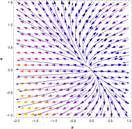
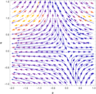
Figure 1: Phase portrait for the dynamical system of Model I, (i) for $n=0.5$; (ii) for $n=\frac{3}{2}$.

Case 2. Matter combined with radiation

Hence the system (27)–(30) becomes

$$p^{\prime}=\frac{4r+3(1-p-q)}{q(1-2n)+2}(q+2p),$$ (34)

$$q^{\prime}=\frac{4r+3(1-p-q)}{q(1-2n)+2}2(1-n)q,$$ (35)

$$r^{\prime}=-2r\left(2+\frac{-4r+3(p+q-1)}{q(1-2n)+2}\right).$$ (36)

Corresponding to this dynamical system, there are three critical points:

Table 2: Critical points, stability conditions and the EoS parameter.

Critical Points	Eigen-Values	$\mathbf{\Omega_{\mathrm{m}}}$	$\mathbf{\Omega_{\mathrm{Q}}}$	$\mathbf{\Omega_{\mathrm{r}}}=r$	$\mathbf{\displaystyle w_{\mathrm{eff}}}$	Stability Condition
$(p,1-p,0)$	$(0,-4,-3)$	$0$	$1$	$0$	$-1$	Stable
$(0,0,0)$	$(3,-1,-3(n-1))$	$1$	$0$	$0$	$0$	Saddle
$(0,0,\frac{1}{4})$	$(4,1,-4(n-1))$	$\frac{3}{4}$	$0$	$\frac{1}{4}$	$\frac{1}{12}$	Unstable for $n\leq 1$, Saddle for $n>1$

* Critical Point $(p,1-p,0)$ :At this point, the curve implies a solution where $\displaystyle w_{mathrm{eff}}=-1$, the universe accelerates, and the effective dark energy component dominates, or $\Omega_{mathrm{Q}}=1$. This solution reflects the behavior of a cosmological constant. The curve has one vanishing eigenvalue and two additional eigenvalues, $-4$ and $-3$. It is one-dimensional. The stability of the curve can be evaluated by examining the signature of non-zero eigenvalues. The point’s curve is therefore continuously stable. Furthermore, since the related Jacobian matrix has a single vanishing eigenvalue, the critical point $(p,1-p,0)$ is non-hyperbolic. We find that the system of equations is asymptotically stable by applying the center manifold theory method.

In this instance, the stable variables are $q,r$, while the central variable is $p$. The corresponding matrices are $A=0$ and $B=\begin{pmatrix}-4&0\\ 0&-3\end{pmatrix}$. The center manifold has now the form $q=h_{1}(p)$ and $r=h_{2}(p)$. The two components of the approximation $\mathcal{N}$ are:

$\mathcal{N}_{1}(h_{1}(p))=h_{1}^{\prime}(p)\frac{4h_{2}(p)+3(1-p-h_{1}(p))}{h_{1}(p)(1-2n)+2}(h_{1}(p)+2p)-\frac{4h_{2}(p)+3(1-p-h_{1}(p))}{h_{1}(p)(1-2n)+2}2(1-n)h_{1}(p),$

$\mathcal{N}_{2}(h_{2}(p))=h_{2}^{\prime}(p)\frac{4h_{2}(p)+3(1-p-h_{1}(p))}{h_{1}(p)(1-2n)+2}(h_{1}(p)+2p)+2h_{2}(p)\left(2+\frac{-4h_{2}(p)+3(p+h_{1}(p)-1)}{h_{1}(p)(1-2n)+2}\right)$

For zeroth approximation:

$\mathcal{N}_{1}(h_{1}(p))=0+\mathcal{O}(p^{2})$

and

$\mathcal{N}_{2}(h_{2}(p))=-\frac{7}{2}+3p+\mathcal{O}(p^{2})$

Therefore the reduced equation gives us

$x^{\prime}=-11p+\mathcal{O}(p^{2})$

This provides the negative linear portion. Thus, according to the central manifold theory, the system of equations (34)-–(36) is stable at the equilibrium point.

* Critical Point $(0,0,0)$: The critical point $(0,0,0)$ signifies a scenario where $\Omega_{\mathrm{m}}=1$, $\Omega_{\mathrm{Q}}=0$, $\Omega_{\mathrm{r}}=0$, and $\displaystyle w_{\mathrm{eff}}=0$, emphasizing the supremacy of matter at the background level. Despite having eigenvalues $(3,-1,-3(n-1))$ for all $n$, this point serves as a saddle. Trajectories pass through this point, subsequently diverging as they approach a late-time stable point. This observation leads us to consider this scenario as a compelling explanation for the formation of structures during the matter-dominated period at background levels.

* Critical Point $(0,0,\frac{1}{4})$: This particular point is characterized by $\Omega_{\mathrm{m}}=\frac{3}{4}$, $\Omega_{\mathrm{Q}}=0$, $\Omega_{\mathrm{r}}=\frac{1}{4}$, and $\displaystyle w_{\mathrm{eff}}=\frac{1}{12}$. It signifies an epoch where matter, radiation, and dark energy coexist. The eigenvalues of the Jacobian matrix at this critical point are $(4,1,-4(n-1))$. For $n\leq 1$, this point proves to be unstable, while for $n>1$, it exhibits saddle-like behavior.

       

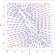
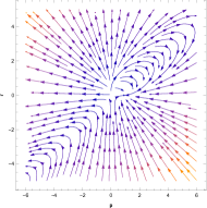
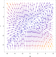
Figure 2: Phase portrait for the dynamical system of Model I, (i)left panel($r=0$ and $n=0.5$); (ii)middle panel($q=0$); (iii)right panel($p=0$ and $n=0.5$).

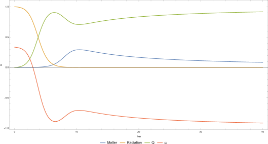
Figure 3: Evolution of matter, radiation, $Q$ and the EoS parameter in the power-law model.

In Fig. 3, the initial phase shows the universe predominantly filled with radiation, gradually diminishing as matter formation progresses, leading to an increase in its relative energy density. Eventually, in the latter stages, the dominance of dark energy initiates and drives the observed acceleration in the universe’s expansion.

The parameter $\displaystyle w_{\mathrm{eff}}$ reflecting the equation of state starts at $\frac{1}{3}$ when radiation dominates the universe entirely. It decreases to zero during the epoch of matter formation, eventually turning negative and reaching its ultimate value of $\displaystyle w_{\mathrm{eff}}=-1$ as dark energy gradually ascends to dominance. This evolution of $\displaystyle w_{\mathrm{eff}}$ delineates the transitions between radiation, matter, and dark energy eras within the cosmic history showcased in Fig. 3.

IV.2 MODEL II : $F(Q)=Qe^{\kappa(\frac{Q_{0}}{Q})}-Q$

In this subsection we consider the exponential model

$$F(Q)=Qe^{\kappa(\frac{Q_{0}}{Q})}-Q,$$ (37)

with having the only one dimensionless parameter $\kappa$. For $\kappa=0$ the model is equivalent to GR without a cosmological constant. The model can fit observations extremely satisfactorily for $\kappa\neq 0$, despite the fact that it does not contain a cosmological constant. Note that $\kappa$ can be eliminated in terms of $\Omega_{m0}$ by using the first Friedmann equation at present. Additionally, because the model tends to GR limit at early times when $Q\gg Q_{0}$, it easily satisfies the BBN constraints [68, 69, 70, 65]. As

$QF_{QQ}=\frac{(p+1)^{2}+p(q-2)+\frac{q^{2}}{4}-1}{p+1}$,

Mathematically, exponential functions are rather straightforward and tractable. They can be used to investigate the fundamental aspects of $f(Q)$ gravity and lead to simple analytical solutions. Exponential forms, which lack new fields or complicated interactions, can imitate some properties of dark energy, such as a accelearting the expansion of the cosmos. Depending on the precise shape of the exponential function, it can be used to explain observational evidence on the cosmic microwave background (CMB) and supernovae that are related to the universe’s accelerating expansion. Exponential $f(Q)$ gravity models have been compared to observational data, and some of them were found to be accurate. These models can offer GR alternatives that are in line with a number of cosmological and astrophysical observations. By changing the exponential model’s parameters, researchers can examine various gravitational dynamics and departures from general relativity.

In summary, exponential models in $f(Q)$ gravity are valuable tools for exploring and testing alternative gravity theories. They offer a framework to investigate the nature of dark energy, the validity of General Relativity, the behavior of gravity on various scales, and the potential connections between dark energy and dark matter. These models contribute to our ongoing efforts to understand the fundamental forces that govern the universe’s behavior.

Case 1. Only matter

The system (22)–(24) becomes

$$p^{\prime}=\frac{3(1-p-q)}{\frac{(2p+q)^{2}}{p+1}-q+2}(q+2p),$$ (38)

$$q^{\prime}=\frac{3(1-p-q)}{(2p+q)^{2}-(y-2)(p+1)}(2p+q)^{2}$$ (39)

In this case, the system has two curves of critical points

Table 3: Critical points, stability conditions and the EoS parameter.

Critical Points	Eigen-Values	$\mathbf{\Omega_{\mathrm{m}}}$	$\mathbf{\Omega_{\mathrm{Q}}}$	$\mathbf{\displaystyle w_{\mathrm{eff}}}$	Stability Condition
$(p,1-p)$	$(-3,0)$	$0$	$1$	$-1$	Stable
$(p,-2p)$	$(3,0)$	$1+p$	$-p$	$0$	Unstable

* Critical Point $(p,1-p)$: The curve at this point is consistent with a solution where the energy density $\Omega_{\mathrm{m}}=0$, indicating that matter does not contribute to the overall energy density of the universe. However, the energy density $\Omega_{\mathrm{Q}}=1$ indicates that dark energy totally controls the universe’s overall energy density. This would suggest that the universe’s apparent accelerated expansion is purely caused by the repelling effects of dark energy, without any major contribution from matter. Indeed, in line with the anticipated behavior resembling that of a cosmological constant, the universe experiences acceleration characterized by $\displaystyle w_{\mathrm{eff}}=-1$.

The curve under examination is one-dimensional, featuring eigenvalues of $0$ and $-3$. Analyzing the non-vanishing eigenvalue, we determine the curve’s stability. Additionally, due to the non-hyperbolic nature of the critical point $(p,1-p)$, the application of center manifold theory confirms the system’s asymptotic stability.

In this case $q$ and $q$ are the central and stable variables respectively. The corresponding matrices are $A=-3$ and $B=0$. Now, the center manifold has the form $p=h(q)$; the approximation $\mathcal{N}$ is given by

$\mathcal{N}(h(q))=h^{\prime}(q)\frac{3(1-h(q)-q)}{u(q)-q+2}u(q)-\frac{3(1-h(q)-q)}{u(q)-q+2}(q+2h(q))$

where $u(q)=\frac{4(h(q)+1)^{2}+4h(q)(q-2)+q^{2}-1}{(h(q)+1)}$ .
For zeroth approximation:

$\mathcal{N}(h(q))=-\frac{3q}{q^{2}-q+2}+\mathcal{O}(q^{2})$.

Therefore the reduced equation is

$q^{\prime}=0+\mathcal{O}(q^{2})$

This gives us the zero constant part. Therefore, the system of equation (38)–(39) is stable but not asymptotically as per the Central Manifold Theory.

Asymptotic stability implies that the system not only remains bounded but also that it eventually settles down to a steady state after experiencing transient behavior. Both stable and asymptotically stable systems remain bounded and do not exhibit unbounded behavior, asymptotically stable systems go a step further by ensuring that perturbations from the equilibrium state converge to zero over time.

In conclusion, the argument summarises the point’s curve $(p,1-p)$, is the dark-energy-dominated universe of the late universe.

* Critical Point $(p,-2p)$: At this point, where $\displaystyle w_{\mathrm{eff}}=0$ and $\Omega_{\mathrm{m}}=1+p$, it represents the dominance of matter at the background level. However, this point is unstable due to the Jacobian matrix’s eigenvalues being $(3,0)$. The energy density configuration $\Omega_{\mathrm{m}}=1+p$ and $\Omega_{\mathrm{Q}}=-p$ suggests that the matter component overwhelmingly constitutes the total energy density of the universe, considering that the value of $p$ is exceptionally small. Consequently, this indicates that the entirety of the energy density is attributed to matter, encompassing both ordinary matter (baryonic matter) and dark matter.

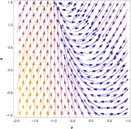
Figure 4: Phase portrait for the dynamical system of Model II

Case 2. Matter combined with radiation

In this case the system (27)–(30) becomes

$$p^{\prime}=\frac{4r+3(1-p-q)}{\frac{(2p+q)^{2}}{(p+1)}-q+2}(q+2p),$$ (40)

$$q^{\prime}=\frac{4r+3(1-p-q)}{\frac{(2p+q)^{2}}{(p+1)}-q+2}\frac{(2p+q)^{2}}{(p+1)},$$ (41)

$$r^{\prime}=-2r\left(2+\frac{-4r+3(p+q-1)}{\frac{(2p+q)^{2}}{(p+1)}-q+2}\right).$$ (42)

In this case, the system has three curves of critical points

Table 4: Critical points, stability conditions, radiation and the EoS parameter.

Critical Points	Eigen-Values	$\mathbf{\Omega_{\mathrm{m}}}$	$\mathbf{\Omega_{\mathrm{Q}}}$	$\mathbf{\Omega_{\mathrm{r}}}=r$	$\mathbf{\displaystyle w_{\mathrm{eff}}}$	Stability Condition
$(p,1-p,0)$	$(-4,-3,0)$	$0$	$1$	$0$	$-1$	Stable
$(p,-2p,0)$	$(3,-1,0)$	$1+p$	$-p$	$0$	$0$	Saddle
$(p,-2p,\frac{(1+p)}{4})$	$(4,1,0)$	$\frac{3}{4}(1+p)$	$-p$	$\frac{(1+p)}{4}$	$\frac{1}{12}$	Unstable

* Critical Point $(p,1-p,0)$ : The curve at this point, the solution depicts the dominance of dark energy component, or $\Omega_{\mathrm{Q}}=1$, where the universe undergoes acceleration characterized by $\displaystyle w_{\mathrm{eff}}=-1$. This behavior closely resembles that of a cosmological constant. It becomes evident that within this scenario, the geometric aspect of the $f(Q)$ model assumes dominance over the critical point. The curve has one vanishing eigenvalue and two other eigenvalues are $-4$ and $-3$. The stability analysis of this point is contingent upon the sign of the non-zero eigenvalues. Consequently, the curve’s point maintains a consistent stability owing to this. Additionally, the critical point $(p,1-p,0)$ is non-hyperbolic. The system of equations achieves asymptotic stability through the application of center manifold theory techniques.

In this case, $r$ is the central variable, while $p,q$ are the stable variables. The corresponding matrices are $A=\begin{pmatrix}-4&0\\ 0&-3\end{pmatrix}$ and $B=0$. The center manifold has now the form $p=h_{1}(r)$ and $q=h_{2}(r)$. The two components of the approximation $\mathcal{N}$ are:

$\mathcal{N}_{1}(h_{1}(r))=h_{1}^{\prime}(r)\left(-2r\left(2+\frac{-4r+3(h_{1}(r)+h_{2}(r)-1)}{\frac{(2h_{1}(r)+h_{2}(r))^{2}}{(h_{1}(r)+1)}-h_{2}(r)+2}\right)\right)-\frac{4r+3(1-h_{1}(r)-h_{2}(r))}{\frac{(2h_{1}(r)+h_{2}(r))^{2}}{(h_{1}(r)+1)}-h_{2}(r)+2}(h_{2}(r)+2h_{1}(r)),$

$\mathcal{N}_{2}(h_{2}(r))=h_{2}^{\prime}(r)\left(-2r\left(2+\frac{-4r+3(h_{1}(r)+h_{2}(r)-1)}{\frac{(2h_{1}(r)+h_{2}(r))^{2}}{(h_{1}(r)+1)}-h_{2}(r)+2}\right)\right)-\left(\frac{4r+3(1-h_{1}(r)-h_{2}(r))}{\frac{(2h_{1}(r)+h_{2}(r))^{2}}{(h_{1}(r)+1)}-h_{2}(r)+2}\right)\left(\frac{(2h_{1}(r)+h_{2}(r))^{2}}{(h_{1}(r)+1)}\right)$

For zeroth approximation:

$\mathcal{N}_{1}(h_{1}(r))=0+\mathcal{O}(r^{2})$

and

$\mathcal{N}_{2}(h_{2}(r))=0+\mathcal{O}(r^{2})$.

Therefore the reduced equation is

$r^{\prime}=-r+\mathcal{O}(r^{2})$

The above equation has the negative linear part. According to the central manifold theory, the set of equations (40)–-(42) is thus asymptotically stable at the equilibrium.

In conclusion, the discussion describes how, in the later stages of the universe, dark energy becomes the most influential force in the background.

* Critical Point $(p,-2p,0)$: The curve of this critical point $(p,-2p,0)$, corresponds to a solution with $\Omega_{\mathrm{m}}=1+p$, $\Omega_{\mathrm{Q}}=-p$ and $\displaystyle w_{\mathrm{eff}}=0$. Note that the value of $p$ is very small, i.e. close to zero. This is the era where the matter component completely dominates the total energy density of the universe. However, it is saddle with eigenvalues $(3,-1,0)$.

* Critical Point $(p,-2p,\frac{(1+p)}{4})$: This position, where $\Omega_{\mathrm{m}}=\frac{3}{4}(1+p)$, $\Omega_{\mathrm{Q}}=-p$, $\Omega_{r}=\frac{(1+p)}{4}$ and $\displaystyle w_{\mathrm{eff}}=\frac{1}{12}$. Since $p$ is very small, this critical curve depicts the era where there is matter, radiations as well as dark energy . The Jacobian matrix’s eigenvalues are $(4,1,0)$, making this point unstable.

       

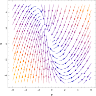
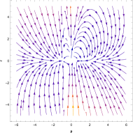
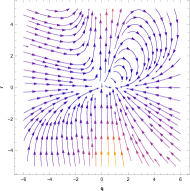
Figure 5: Phase portrait for the dynamical system of Model II, (i)left panel($r=0$); (ii)middle panel($q=0$); (iii)right panel($p=0$).

IV.3 MODEL III : $F(Q)=\beta+\kappa\log Q-Q$

$$F(Q)=\beta+\kappa logQ-Q$$ (43)

the logarithmic model, has two parameters, $\beta$ and $\kappa$. This model also fits in the BBN requirements [68, 69, 70, 65] and can explain the acceleration in the late universe. As,

$QF_{QQ}=\frac{(q-2)}{2}$

One of the significant applications of $f(Q)$ gravity models, including logarithmic ones, is their potential to explain the accelerated expansion of the universe, which is attributed to dark energy in the standard cosmological model. Observations and experiments that probe gravitational interactions on cosmological scales can be compared with the predictions of these models. Any deviations from GR in favor of logarithmic $f(Q)$ gravity could provide valuable insights into the nature of gravity itself. Also they can have profound consequences for the evolution of the universe. They can influence the dynamics of cosmic structure formation, the cosmic microwave background radiation, and the growth of large-scale structures. Logarithmic models allow for specific predictions that can be tested through various astrophysical and cosmological observations. Comparing the predictions of logarithmic $f(Q)$ gravity with these observations can help determine its validity and distinguish it from GR. By modifying the gravitational interactions on galactic and cosmological scales, these models aim to account for observed phenomena like galactic rotation curves without the need for dark matter particles. Logarithmic models in $f(Q)$ gravity also have implications for the early universe, such as inflationary cosmology. They can influence the dynamics of the early universe and leave imprints on the cosmic microwave background, providing opportunities to test these models in the context of the Big Bang.

In summary, logarithmic models in $f(Q)$ gravity are important tools for exploring and testing alternative gravity theories that can potentially address some of the unresolved questions and anomalies in astrophysics and cosmology. They offer a framework to investigate the nature of dark energy, the validity of General Relativity, and the behavior of gravity on various scales, from galaxies to the entire universe.

Case 1. Only matter

In this case, the system (22)–(24) becomes.

$$p^{\prime}=\frac{3(1-p-q)}{q-2}(q+2p),$$ (44)

$$q^{\prime}=\frac{3(1-p-q)}{q-2}2(q-2),$$ (45)

There is only one corresponding critical point.

Table 5: Critical Points, Stability Conditions and EoS parameter.

Critical Points	Eigen-Values	$\mathbf{\Omega_{\mathrm{m}}}$	$\mathbf{\Omega_{\mathrm{Q}}}$	$\mathbf{\displaystyle w_{\mathrm{eff}}}$	Stability Condition
$(p,1-p)$	$(-3,0)$	$0$	$1$	$-1$	Stable

* Critical Point $(p,1-p)$: The curve at this point is consistent with the energy density $\Omega_{\mathrm{m}}=0$ solution, proving that matter has no effect on the universe’s overall energy density. According to the energy density $\Omega_{\mathrm{Q}}=1$, dark energy entirely controls the overall energy density of the universe. This would imply that the universe accelerates with $\displaystyle w_{\mathrm{eff}}=-1$, which is compatible with the behaviour of a cosmological constant, and that the apparent rapid expansion is solely due to the repulsive effects of dark energy, with no contribution from matter.

The critical point $(p,1-p)$ is non-hyperbolic and $-3$ is the other eigenvalue. Looking at the non-vanishing eigenvalue, the curve is stable. Also, we found that the system of equations is asymptotically stable using the center manifold theory.

In this case $p$ and $q$ are the stable and center variables respectively. The corresponding matrices are $A=-3$ and $B=0$. The center manifold has now the form $p=h(q)$; the approximation $\mathcal{N}$ is given by

$\mathcal{N}(h(q))=h^{\prime}(q)\frac{3(1-h(q)-q)}{u(q)-q+2}u(q)-\frac{3(1-h(q)-q)}{u(q)-q+2}(q+2h(q))$

where $u(q)=\frac{4(h(q)+1)^{2}+4h(q)(q-2)+q^{2}-1}{(h(q)+1)}$
For zeroth approximation:

$\mathcal{N}(h(q))=-\frac{3q}{q-2}+\mathcal{O}(q^{2})$

Therefore the reduced equation is

$q^{\prime}=-18+\mathcal{O}(q^{2})$

This provides us with the negative constant portion. According to the central manifold theory, the system of equations (44)–(45) is asymptotically stable at the equilibrium point.

The argument summarises the point’s curve $(p,1-p)$, which is the late universe’s dark-energy-dominated universe.

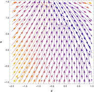
Figure 6: Phase portrait for the dynamical system of Model III.

Case 2. Matter combined with radiation

In this case, the system (27)–(30) becomes.

$$p^{\prime}=\frac{4r-3(p+q-1)}{q-2}(q+2p),$$ (46)

$$q^{\prime}=\frac{4r-3(p+q-1)}{q-2}2(q-2),$$ (47)

$$r^{\prime}=-2r(2+\frac{-4r+3(p+q-1)}{q-2}).$$ (48)

The above dynamical system has one critical point.

Table 6: Critical points, stability conditions and the EoS parameter.

Critical Points	Eigen-Values	$\mathbf{\Omega_{\mathrm{m}}}$	$\mathbf{\Omega_{\mathrm{Q}}}$	$\mathbf{\Omega_{\mathrm{r}}=r}$	$\mathbf{\displaystyle w_{\mathrm{eff}}}$	Stability Condition
$(p,1-p,0)$	$(-4,-3,0)$	$0$	$1$	$0$	$-1$	Stable

* Critical Point $(p,1-p,0)$ : The curve at this point is consistent with the energy density $\Omega_{\mathrm{m}}=0$ solution, proving that matter has no effect on the universe’s overall energy density. According to the energy density $\Omega_{\mathrm{Q}}=1$, dark energy entirely controls the overall energy density of the universe. This would imply that the universe accelerates with $\displaystyle w_{\mathrm{eff}}=-1$, which is compatible with the behaviour of a cosmological constant, and that the apparent rapid expansion is solely due to the repulsive effects of dark energy, with no contribution from matter. The curve has one vanishing eigenvalue and two additional eigenvalues, $-4$ and $-3$. It is one-dimensional. Examining the non-zero eigenvalue signature allows one to determine whether the curve is stable. As a result, the curve at the point is constantly stable. Furthermore, since the related Jacobian matrix has just one vanishing eigenvalue, the critical point $(p,1-p,0)$ is non-hyperbolic. We find that the system of equations is asymptotically stable by applying the center manifold theory method.

The central variable in this instance is $r$, and the stable variables are $p,q$. The corresponding matrices are $A=\begin{pmatrix}-4&0\\ 0&-3\end{pmatrix}$ and $B=0$. Now, the center manifold has the form $p=h_{1}(r)$ and $q=h_{2}(r)$; the approximation $\mathcal{N}$ has two components:

$\mathcal{N}_{1}(h_{1}(r))=h_{1}^{\prime}(r)\left(-2r\left(2+\frac{-4r+3(h_{1}(r)+h_{2}(r)-1)}{\frac{(2h_{1}(r)+h_{2}(r))^{2}}{(h_{1}(r)+1)}-h_{2}(r)+2}\right)\right)-\left(\frac{4r+3(1-h_{1}(r)-h_{2}(r))}{\frac{(2h_{1}(r)+h_{2}(r))^{2}}{(h_{1}(r)+1)}-h_{2}(r)+2}\right)\left(h_{2}(r)+2h_{1}(r)\right),$

$\mathcal{N}_{2}(h_{2}(r))=h_{2}^{\prime}(r)\left(-2r\left(2+\frac{-4r+3(h_{1}(r)+h_{2}(r)-1)}{\frac{(2h_{1}(r)+h_{2}(r))^{2}}{(h_{1}(r)+1)}-h_{2}(r)+2}\right)\right)-\left(\frac{4r+3(1-h_{1}(r)-h_{2}(r))}{\frac{(2h_{1}(r)+h_{2}(r))^{2}}{(h_{1}(r)+1)}-h_{2}(r)+2}\right)\left(\frac{(2h_{1}(r)+h_{2}(r))^{2}}{(h_{1}(r)+1)}\right)$

For zeroth approximation:

$\mathcal{N}_{1}(h_{1}(r))=0+\mathcal{O}(r^{2})$

and

$\mathcal{N}_{2}(h_{2}(r))=-8r-6+\mathcal{O}(r^{2})$.

Therefore the reduced equation gives us

$r^{\prime}=-6r+\mathcal{O}(r^{2})$

This provides us with the negative constant portion. According to the central manifold theory, the system of equations (46)-(48) is asymptotically stable at the equilibrium point.

The discussion concludes with a background-level description of the dark-energy-dominated late universe.

       

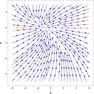
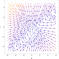
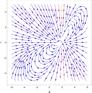
Figure 7: Phase portrait for the dynamical system of Model III, (i)left panel($r=0$); (ii)middle panel($q=0$); (iii)right panel($p=0$).

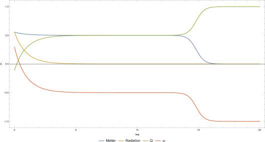
Figure 8: Evolution of matter, radiation, $Q$ and the EoS parameter in the logarithmic model.

In Fig. 8, it can be seen that the universe is initially completely filled with radiation, which subsequently gradually decreases and matter begins to form, increasing the relative energy density. So $\displaystyle w_{\mathrm{eff}}$ behaves similarly to the energy density of radiation until dark energy enters the picture. Later on, dark energy takes over and causes the accelerated expansion of the universe that we are currently observing. The parameter $\displaystyle w_{\mathrm{eff}}$ starts at $-0.55$ when the universe was totally dominated by radiation, then drops during the matter formation era, then gets negative when dark energy begins to dominate, and finally reaches the value of $\displaystyle w_{\mathrm{eff}}$, which is $-1$.

V Conclusions and Discussions

In the current study, we coupled the dynamical system analysis of the background equations to test the validity of the findings using an independent approach. The flat FLRW metric is regarded to be the best description of the universe. This research was inspired by the fact that higher-order symmetric teleparallel equivalent of general relativity, i.e, $f(Q)$ gravity-based cosmological models are particularly effective at fitting observable datasets at both background levels. Following the conversion of the background equations into an autonomous framework, our investigation on prevalent models found in literature, concentrating on the power-law, exponential, and logarithmic higher-curvature gravity models augmented by a boundary terms. In the work, we have considered two cases: “Case I- only matter” and “Case II- Matter combined with radiation without interaction” for each model.

In the power-law model represented by $f(Q)=Q+\kappa(\frac{Q}{Q_{0}})^{n}$, the scenario involving only matter revealed two critical points. Among these, the equilibrium point at $(p,1-p)$ emerged as asymptotically stable through the application of center manifold theory. This critical point’s significance lies in asserting the dominance of dark energy during the later phases of the universe. It signifies that the universe’s accelerated expansion solely stems from the repulsive effects of dark energy, without any contribution from matter. On the other hand, the point $(0,0)$ behaved as a saddle point for $n>1$ and proved to be unstable for $n\leq 1$. This specific point denotes the epoch where matter formation reaches completion. Our depiction of phase portraits in Fig. 1 provides a visual representation, enhancing the comprehension of these behaviors at these critical points.

In the scenario involving matter combined with radiation without any interaction, our analysis unveiled three critical points, among which the point $(p,1-p,0)$ emerged as asymptotically stable, employing center manifold theory. This specific point on the curve signifies a solution where the dominance of an effective dark energy component leads to the universe accelerating with $\displaystyle w_{\mathrm{eff}}=-1$, aligning with the behavior akin to a cosmological constant. Contrarily, the point $(0,0,0)$ exhibited saddle-like behavior with eigenvalues $(3,-1,-3(n-1)$ across all $n$ values. Our observations indicate trajectories converging towards a stable late-time point, passing through it, and subsequently diverging from it. We hypothesize that this particular point might serve as the most plausible candidate for elucidating the development of structures during the matter-dominated epoch at background levels. The point $(0,0,\frac{1}{4})$ was found to be saddle for $n>1$ and unstable for $n\leq 1$. This critical point depicts the period where matter, radiation, and dark energy are present together. Additionally, we plotted phase portraits in Fig. 2, which provides a clearer representation of the behavior at those points. Fig. 3 illustrates how the energy density parameter can be used to display the behavior of dark energy versus $\ln a$ in order to comprehend its dominance in various ages of the cosmos.

In the exponential model $f(Q)=Qe^{\kappa(\frac{Q_{0}}{Q})}$, for matter case, two critical points were obtained, out of which the point $(p,1-p)$ was found to be asymptotically stable by using center manifold theory with the eigen-values $(-3,0)$ and the point $(p,-2p)$ was unstable. The critical point $(p,1-p)$ indicates that dark energy predominates in the late universe and that matter has no impact on its repulsive effects, which are responsible for the universe’s observable accelerated expansion. This critical point depicts the era of the late-time-dark-energy dominated universe. The critical point $(p,-2p)$ depicts the era where the matter component completely dominates the total energy density of the universe.

For matter combined with radiation case i.e case II, there were three critical points, out of which $(p,1-p,0)$ point with the eigen-value $(-4,-3,0)$ was found to be asymptotically stable at equilibrium points by using center manifold theory. The curve at this point depicts a solution where the universe accelerates with $\displaystyle w_{\mathrm{eff}}=-1$ and the effective dark energy component predominates, which is in line with the behavior of a cosmological constant. The points $(p,-2p,0)$ and $(p,-2p,\frac{(1+p)}{4})$ were saddle and unstable respectively. In phase portrait, Figs. 4 and 5, the behavior at those points is well depicted.

In the logarithmic model characterized by $f(Q)=\beta+\kappa\log Q$, we encountered a single critical point for both scenarios: the matter-only case yielded $(p,1-p)$, while the matter combined with radiation scenario resulted in $(p,1-p,0)$. Utilizing center manifold theory, our analysis indicated that in both cases, these points proved to be asymptotically stable at their respective equilibrium states. Moreover, these critical points corresponded to curves indicative of matter dominance and the prevalence of the geometric aspect within the higher-curvature gravity model accompanied by a boundary term. In Figs. 6 and 7, we illustrated phase portraits to offer a more detailed insight into the behaviors exhibited at these critical points. To further elucidate the dominance of dark energy across different cosmic eras, we delved into the energy density parameter. In Fig. 8, we demonstrated the behavior of this parameter plotted against $\ln a$, providing a comprehensive understanding of dark energy’s prevalence throughout various epochs of the universe.

As a concluding note, this study successfully demonstrates stability and acceleration phases within the universe’s evolution without the inclusion of an“unobserved” entity like dark energy. The models explored in this article portray these phenomena without necessitating the introduction of such an additional component, offering valuable insights into cosmic dynamics while relying solely on observable quantities.

This research could be extended by taking into account more higher-curvature gravity with boundary term models that meet the BBN (Big-Bang Nucleosynthesis) constraints and all viability requirements. In addition to this, other categories of modification such as $f(Q,T)$ or Weyl-type theories might be taken into account, and further applications of dynamical system analysis could be made as well as stability analyses for such cases could be carried out. Several forms of linear and nonlinear interactions could also be studied with modification in the gravity.

References

- [1] S. Perlmutter et al. [Supernova Cosmology Project], Astrophys. J. 517, 565-586 (1999).
- [2] A. G. Riess et al. [Supernova Search Team], Astron. J. 116, 1009-1038 (1998).
- [3] A. G. Riess et al. [Supernova Search Team], Astrophys. J. 607, 665-687 (2004).
- [4] N. Aghanim et al. [Planck], Astron. Astrophys. 641, A6 (2020) [erratum: Astron. Astrophys. 652, C4 (2021)].
- [5] T. Koivisto and D. F. Mota, Phys. Rev. D 73, 083502 (2006).
- [6] S. F. Daniel, R. R. Caldwell, A. Cooray and A. Melchiorri, Phys. Rev. D 77, 103513 (2008).
- [7] D. J. Eisenstein et al. [SDSS], Astrophys. J. 633, 560-574 (2005).
- [8] E. J. Copeland, M. Sami and S. Tsujikawa, Int. J. Mod. Phys. D 15, 1753-1936 (2006).
- [9] T. Padmanabhan, Gen. Rel. Grav. 40, 529-564 (2008).
- [10] R. Durrer and R. Maartens, Gen. Rel. Grav. 40, 301-328 (2008).
- [11] K. Bamba, S. Capozziello, S. Nojiri and S. D. Odintsov, Astrophys. Space Sci. 342, 155-228 (2012).
- [12] R. Kase and S. Tsujikawa, Int. J. Mod. Phys. D 28, no.05, 1942005 (2019).
- [13] N. Aghanim et al. [Planck], Astron. Astrophys. 641, A6 (2020) [erratum: Astron. Astrophys. 652, C4 (2021)].
- [14] B. Ratra and P. J. E. Peebles, Phys. Rev. D 37, 3406 (1988).
- [15] R. R. Caldwell, R. Dave and P. J. Steinhardt, Phys. Rev. Lett. 80, 1582-1585 (1998).
- [16] R. R. Caldwell, Phys. Lett. B 545, 23-29 (2002).
- [17] B. Feng, X. L. Wang and X. M. Zhang, Phys. Lett. B 607, 35-41 (2005).
- [18] R. Bean, D. J. H. Chung and G. Geshnizjani, Phys. Rev. D 78, 023517 (2008).
- [19] D. Langlois, Int. J. Mod. Phys. D 28, no.05, 1942006 (2019).
- [20] H. A. Buchdahl, Mon. Not. Roy. Astron. Soc. 150, 1 (1970).
- [21] T. P. Sotiriou and V. Faraoni, Rev. Mod. Phys. 82, 451-497 (2010).
- [22] A. A. Starobinsky, Phys. Lett. B 91, 99-102 (1980).
- [23] D. J. Brooker, S. D. Odintsov and R. P. Woodard, Nucl. Phys. B 911, 318-337 (2016).
- [24] Q. G. Huang, JCAP 02, 035 (2014).
- [25] S. Nojiri, S. D. Odintsov and V. K. Oikonomou, Phys. Rept. 692, 1-104 (2017).
- [26] S. Capozziello and M. De Laurentis, Phys. Rept. 509, 167-321 (2011).
- [27] A. De Felice and S. Tsujikawa, Living Rev. Rel. 13, 3 (2010).
- [28] S. Nojiri and S. D. Odintsov, Phys. Rept. 505, 59-144 (2011).
- [29] S. Arai, K. Aoki, Y. Chinone, R. Kimura, T. Kobayashi, H. Miyatake, D. Yamauchi, S. Yokoyama, K. Akitsu and T. Hiramatsu, et al. PTEP 2023, no.7, 072E01 (2023).
- [30] T. Harko, F. S. N. Lobo, S. Nojiri and S. D. Odintsov, Phys. Rev. D 84, 024020 (2011).
- [31] S. Capozziello and M. De Laurentis, Phys. Rept. 509, (2011) 167-321.
- [32] T. Clifton, P. G. Ferreira, A. Padilla and C. Skordis, Phys. Rept. 513, 1-189 (2012).
- [33] A. Joyce, B. Jain, J. Khoury and M. Trodden, Phys. Rept. 568, 1-98 (2015).
- [34] M. Koussour, S. H. Shekh, A. Hanin, Z. Sakhi, S. R. Bhoyer and M. Bennai, Class. Quant. Grav. 39, no.19, 195021 (2022).
- [35] R. Ferraro and F. Fiorini, Phys. Rev. D 75, 084031 (2007).
- [36] Y. F. Cai, S. Capozziello, M. De Laurentis and E. N. Saridakis, Rept. Prog. Phys. 79, no.10, 106901 (2016).
- [37] S. Bahamonde, K. F. Dialektopoulos, C. Escamilla-Rivera, G. Farrugia, V. Gakis, M. Hendry, M. Hohmann, J. Levi Said, J. Mifsud and E. Di Valentino, Rept. Prog. Phys. 86, no.2, 026901 (2023).
- [38] J. Beltrán Jiménez, L. Heisenberg and T. Koivisto, Phys. Rev. D 98, no.4, 044048 (2018).
- [39] J. Beltrán Jiménez, L. Heisenberg, T. S. Koivisto and S. Pekar, Phys. Rev. D 101, no.10, 103507 (2020).
- [40] L. Heisenberg, [arXiv:2309.15958 [gr-qc]].
- [41] S. Mandal, P. K. Sahoo and J. R. L. Santos, Phys. Rev. D 102, no.2, 024057 (2020).
- [42] S. Mandal, D. Wang and P. K. Sahoo, Phys. Rev. D 102, 124029 (2020).
- [43] T. Harko, T. S. Koivisto, F. S. N. Lobo, G. J. Olmo and D. Rubiera-Garcia, Phys. Rev. D 98, no.8, 084043 (2018).
- [44] N. Dimakis, A. Paliathanasis and T. Christodoulakis, Class. Quant. Grav. 38, no.22, 225003 (2021).
- [45] M. Koussour, S. H. Shekh and M. Bennai, JHEAp 35, 43-51 (2022).
- [46] M. Koussour, S. H. Shekh and M. Bennai, Phys. Dark Univ. 36, 101051 (2022).
- [47] S. D. Odintsov and V. K. Oikonomou, Phys. Rev. D 96, no.10, 104049 (2017).
- [48] S. D. Odintsov, V. K. Oikonomou and P. V. Tretyakov, Phys. Rev. D 96, no.4, 044022 (2017).
- [49] M. Hohmann, L. Jarv and U. Ualikhanova, Phys. Rev. D 96, no.4, 043508 (2017).
- [50] S. D. Odintsov and V. K. Oikonomou, Phys. Rev. D 98, no.2, 024013 (2018).
- [51] S. D. Odintsov and V. K. Oikonomou, Class. Quant. Grav. 36, no.6, 065008 (2019).
- [52] S. Santos Da Costa, F. V. Roig, J. S. Alcaniz, S. Capozziello, M. De Laurentis and M. Benetti, Class. Quant. Grav. 35, no.7, 075013 (2018).
- [53] P. Shah, G. C. Samanta and S. Capozziello, Int. J. Mod. Phys. A 33, no.18n19, 1850116 (2018).
- [54] P. Shah and G. C. Samanta, Eur. Phys. J. C 79, no.5, 414 (2019).
- [55] Ellis, George Francis Rayner, and John Wainwright, eds. Dynamical systems in cosmology. Cambridge University Press, 1997.
- [56] A. A. Coley, “Dynamical systems and cosmology,” Kluwer, (2003).
- [57] J. de Haro, S. Nojiri, S. D. Odintsov, V. K. Oikonomou and S. Pan, Phys. Rept. 1034, 1-114 (2023).
- [58] M. Nakahara, “Geometry, topology and physics”, (2003).
- [59] W. Khyllep, J. Dutta, S. Basilakos and E. N. Saridakis, Phys. Rev. D 105, no.4, 043511 (2022).
- [60] P. Vishwakarma and P. Shah, Int. J. Mod. Phys. D 32, no.11, 2350071 (2023)
- [61] W. Khyllep, J. Dutta, E. N. Saridakis and K. Yesmakhanova, Phys. Rev. D 107, no.4, 044022 (2023).
- [62] P. Shah and G. C. Samanta, Int. J. Mod. Phys. A 35, no.22, 2050124 (2020).
- [63] J. Beltrán Jiménez, L. Heisenberg and T. S. Koivisto, JCAP 08, 039 (2018).
- [64] G. N. Gadbail, S. Arora and P. K. Sahoo, Phys. Lett. B 838, 137710 (2023).
- [65] F. K. Anagnostopoulos, V. Gakis, E. N. Saridakis and S. Basilakos, Eur. Phys. J. C 83, no.1, 58 (2023).
- [66] S. Bahamonde, C. G. Böhmer, S. Carloni, E. J. Copeland, W. Fang and N. Tamanini, Phys. Rept. 775-777, 1-122 (2018).
- [67] N. Tamanini, “Dynamical systems in dark energy models,” (2014).
- [68] R. H. Cyburt, B. D. Fields, K. A. Olive and T. H. Yeh, Rev. Mod. Phys. 88, 015004 (2016).
- [69] J. D. Barrow, S. Basilakos and E. N. Saridakis, Phys. Lett. B 815, 136134 (2021).
- [70] P. Asimakis, S. Basilakos, N. E. Mavromatos and E. N. Saridakis, Phys. Rev. D 105, no.8, 084010 (2022).
- [71] F. K. Anagnostopoulos, S. Basilakos and E. N. Saridakis, Phys. Lett. B 822, 136634 (2021).