Search for Long-lived Particles at Future Lepton Colliders Using Deep Learning Techniques

Abstract

Long-lived particles (LLPs) provide an unambiguous signal for physics beyond the Standard Model (BSM). They have a distinct detector signature, with decay lengths corresponding to lifetimes of around nanoseconds or longer. Lepton colliders allow LLP searches to be conducted in a clean environment, and such searches can reach their full physics potential when combined with machine learning (ML) techniques. In the case of LLPs searches from Higgs decay in $e^{+}e^{-}\to ZH$, we show that the LLP signal efficiency can be improved up to 99% with an LLP mass around 50 GeV and a lifetime of approximately $1$ nanosecond, using deep neural network based approaches. The signal sensitivity for the branching ratio of Higgs decaying into LLPs reaches $1.2\times 10^{-6}$ with a statistics of $4\times 10^{6}$ Higgs.

I Introduction

In 2012, the discovery of the Higgs boson completed the final piece of the Standard Model (SM). On one hand, SM predictions match almost all experimental observations remarkably well. On the other hand, SM fails to address some key questions in the evolution of the universe, such as the existence of dark matter, the matter-antimatter imbalance puzzle and the origin of the neutrino mass. Therefore, the experimental search for new physics beyond the Standard Model (BSM) is both intriguing and necessary. So far, BSM signals remain elusive despite of numerous efforts. This typically means that either the new physics requires a higher energy threshold than the currently available experimental energy or that the coupling strength between SM and BSM particles is too small to produce a statistically significant number of observable signals. However, an alternative explanation is that BSM particles have long lifetimes and therefore can escape the detector without being detected. These BSM particles are often referred to as long-lived particles (LLPs). Recently, experimental searches for LLPs have become increasingly active. It should be noted that there are no widely-used and common definitions for LLPs and their lifetimes can vary in a wide range. In this paper we focus on LLPs produced via the rare decay of the Higgs boson, which is defined via the process $e^{+}e^{-}\to ZH(Z\to\text{inclusive},H\to X_{1}+X_{2}$). A Lepton collider can be an ideal factory for the Higgs boson, for example the proposed Circular Electron and Positron Collider (CEPC) [1, 2] aims to produce a vast amount of Higgs bosons by electron-positron annihilation at the center-of-mass energy $\sqrt{s}=240$ GeV. Fig. 1 illustrates Feynman diagrams for the LLP production process from the Higgs decay. The Higgs particle can decay into LLPs via two decay modes with two jets (type I signal) or four jets (type II signal) in the final state [42], where the neutrally charged LLPs ($X_{1}$, $X_{2}$) have identical masses and lifetimes ranging from $10^{-3}$ to $10^{2}$ nano seconds approximately. After production, LLPs can largely escape detection by the inner detector and decay into SM particles when they reach the outer detector, which can be an electromagnetic or hadronic calorimeter, or an external detector positioned at a significant distance from the interaction point.

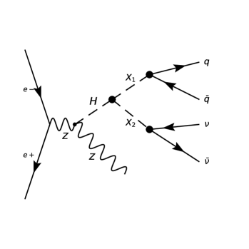
Figure 1: Feynman diagrams of LLP production and decay. Two Feynman diagrams are presented illustrating the generation of long-lived particles (LLPs), denoted as $X_{1}$ and $X_{2}$, through the Higgsstrahlung mechanism. On the left, the diagram shows the production of $X_{1}$ and $X_{2}$ followed by their subsequent decay into a $\nu\bar{\nu}$ pair and a $q\bar{q}$ pair, respectively, resulting in two jets. On the right, both $X_{1}$ and $X_{2}$ decay into $q\bar{q}$ pairs, leading to the four jets final state.

LLPs are sensitive probes to BSM physics, such as supersymmetry (SUSY) theory [3, 4] or dark matter models [5, 6, 7]. They can also help explain the matter-antimatter asymmetry [8, 9, 10] and the neutrino mass hierarchy [11, 12]. In experiment, LLPs often have long decay lengths and leave distinct detector signatures such as displaced vertices or jets inside detectors. Extensive experimental searches for LLPs have been made at various experiments, such as ATLAS [13], CMS [14], and LHCb [15], as well as Belle II [16], BESIII [17], Babar [18]. However, no positive discoveries have been reported so far. There could be a number of reasons for the absence of LLPs signals, low signal-over-background ratio and complexity in event reconstruction with displaced objects are two major ones. In this paper we present a novel method utilizing deep learning techniques to overcome these hurdles. Such techniques can be applied directly to low-level detector information without the need to fully reconstruct the whole event. A deep learning based algorithm has been developed to learn comprehensive LLPs topologies and kinematic features that can distinguish LLPs from various SM backgrounds with high efficiencies and extremely low fake rates. The algorithm has been trained with full simulation Monte Carlo (MC) samples corresponding to an integrated luminosity of $20.0\text{~{}ab}^{-1}$, including LLPs signal samples generated using the event generator MadGraph 3.0.1 [19], and background samples corresponding to $e^{+}e^{-}\to q\bar{q}$, $e^{+}e^{-}\to Z/W$ and $e^{+}e^{-}\to ZH\to\text{inclusive}$ processes generated using the event generator Whizard 1.95 [20, 21]. Other minor backgrounds such as pileup background and cosmic ray background have also been studied and found to be negligible in this analysis.

II Method

General Analysis Strategy

After taking into detector effects, we apply a clustering algorithm to the energy, position, and time of the detector hits. Subsequently, we adopt an ML-based analysis strategy by feeding the clustered hits information into advanced neural networks for multi-label classification. All hit energies have been calibrated using MC samples fully simulated under CEPC conceptual design [24, 34, 35]. The energy resolution for the electromagnetic calorimeter is at $16\%/\sqrt{E/\text{GeV}}\oplus 1\%$, and for the hadronic calorimeter and muon detector it is at $60\%/\sqrt{E/\text{GeV}}\oplus 1\%$. The hit time resolution is set to be 1 nanosecond. Since the ML-based analyses cluster hits at a coarse scale of several centimeters, the finer hit position resolution provided by the detector becomes less critical because the clustering process effectively averages out the hit positions over larger areas.

We define two classifications for the dominating SM backgrounds: the 2-fermion background accounting for $e^{+}e^{-}\rightarrow q\bar{q}$ and $e^{+}e^{-}\to ZH\to\text{inclusive}$ processes, and the 4-fermion background including $e^{+}e^{-}\rightarrow W/Z$ and $e^{+}e^{-}\to ZH\to\text{inclusive}$ processes. We define three classifications for the LLPs signal according to the number of detectable LLPs  [43]: 0, 1, 2. After training with MC simulations, we apply the trained neural networks to statistically independent MC samples to obtain five classification outputs. These outputs serve as inputs of the XGBoost algorithm [36] to further enhance the signal over background discrimination. A final selection is placed on the XGBoost discriminant output to reject all backgrounds and calculate the signal yield.

After the discriminant selection, we employ a toy model to generate 10000 pseudo-experiments based on the predicted signal yields under the zero background condition. We then build a test statistics with the likelihood ratio method [37] to determine 95% C.L. upper limits on $\mathcal{B}(H\rightarrow\text{LLPs})$. A parameter $\epsilon_{V}$ is defined as the ratio $\frac{BR(X\rightarrow\nu\bar{\nu})}{BR(X\rightarrow q\bar{q})}$. $\epsilon_{V}$ can be treated as a fixed parameter or floating parameter. The latter represents a more model-independent approach.

Convolutional Neural Network

For the CNN approach, each event with raw detector hits is transformed into a two-channel image with $200\times 200$ pixels in $(R,\phi)$, where $R$ represents the distance of the position of the hits to the interaction point ($0-6$ m), and $\phi$ represents the azimuthal angle of the hits ($0-2\pi$). The first channel (energy channel) represents a sum of all hits energies in a pixel. The second channel (time channel) represents the time difference ($\Delta t$) associated with the most energetic hit in a pixel as shown in Eq. 1.

$$\Delta t=t_{\text{hit},\text{maxE}}-r_{\text{hit},\text{maxE}}/c$$ (1)

$t_{\text{hit},\text{maxE}}$ is the time of the hit with the maximum energy in a pixel, $r_{\text{hit},\text{maxE}}$ is the Euclidean distance from the interaction point to hit location, and $c$ is the speed of light in vacuum. A selection of hits energy larger than $0.1$ GeV is placed to suppress contributions from extremely low energy hits of secondary particles. Figure 2 shows images of hits for signal and background events. A larger circle indicates a higher energy deposition and a darker color represents a smaller time difference. The event images illustrate the discriminating power of CNN to separate LLPs signals with displaced energies or objects from SM backgrounds. By feeding event images to ResNet18 neural networks [22] shown in Fig. 3, a multi-label classification is performed. The CNN model is trained using 5 GPUs with a batch size of 256 per GPU. The learning rate is adaptively set, beginning at $10^{-4}$ and progressively decreasing to $10^{-6.5}$. The training employs the Adam optimizer with a weight decay of 0.01. The training duration is set at 10 epochs, and the model’s final configuration is determined by the epoch that achieves the lowest validation loss. The distributions of the training and testing losses for CNN are shown in Sec. 1.3 in ”Supplementary Information”.

(a)

(b)

Figure 2: Event visualization of CNN. CNN event images for the Type-I signal (left) and the Type-II signal (right) with backgrounds. Circles represent detector hits in the calorimeter and squares represent detector hits inside the tracker. Darker pixels represent hits with smaller time differences, and bigger pixels represent hits with larger energy. The decay vertex of LLPs is marked with a star symbol.

Figure 3: Network structure of CNN-based classification. The ResNet18 neural network architecture, consisting of two convolutional layers, followed by four ResNet blocks, an average pooling layer, and an output layer for classifications.

Graph Neural Network

For the GNN approach, the raw calorimeter hits and tracker hits belonging to an event are clustered and fed into a heterogeneous event graph with both the calorimeter-type and tracker-type of nodes. The nodes of the same detector type are fully connected to construct edges. To perform the hits clustering in the calorimeter, we first identify the most energetic calorimeter hit and group it together with its neighboring hits that are within a spatial distance of $50~{}mm$. We require the number of neighboring hits larger than 3 and the total number of hits in a cluster larger than 10. We then iterate this procedure for all hits in an event to construct the calorimeter-type nodes. All hits failing the requirements are not clustered and excluded from the GNN. The momentum $p$ of each calorimeter hit is defined as parallel to its position: $p_{i}=\frac{i}{r}E$, where $i$ represents the position along the $x$, $y$, or $z$ axis, with $z$ as the beam line direction, $x$ and $y$ in the transverse plane, and $y$ pointing towards the ground. $r$ is the radial distance $r=\sqrt{x^{2}+y^{2}+z^{2}}$, and $E$ is the hit’s energy. The tracker hits are binned into $5~{}\times~{}6$ blocks based on their R-$\phi$ positions. In each block, the tracker hits are clustered into a tracker-type node taking an arithmetic average of all hits positions. The definitions of nodes and edges for the GNN event graph are summarized in Table 1.

Event graphs are then input into a GNN-based heterogeneous architecture, as illustrated in Fig. 4. Features of different types of nodes and edges are first embedded into a high-dimension latent space and then forwarded to a Heterogeneous Detector Information Block (HDIB). The HDIB consists of two Detector Information Blocks (DIBs) [38][39] and two multilayer perceptrons (MLPs). The HDIB adopts a parameter sharing design between the tracker and the calorimeter types, specifically tailored for integrating information from different types of detectors. After the total $L$ layers of HDIBs, the final node embeddings of the tracker and the calorimeter are aggregated and forwarded to the decode layer to form the classification scores.

The GNN training is performed with 8 GPUs and the batch size is 256 per GPU. The initial learning rate is $10^{-4}$, a dropout rate of 0.1 is used to avoid overfitting. The cross-entropy loss is minimized using the Adam optimizer without weight decay. The GNN model is trained with 30 epochs, and the network is validated at the end of each epoch. The model demonstrating the minimum validation loss value on the validation dataset is then applied to the final test dataset. The distributions of the training and testing losses for GNN are shown in Sec. 1.3 in ”Supplementary Information”.

Table 1: Node and edge features defined in the heterogeneous graph.

Features	Variable	Definition
calorimeter type node $i$	$|x_{i}^{\mu}|$	the space-time interval
	$|p_{i}^{\mu}|$	the invariant mass
	$N_{i}$	the number of hits
	$\eta_{i}$	$\frac{1}{2}\ln{\frac{1+\frac{p_{z}}{p}}{1-\frac{p_{z}}{p}}}$
	$\phi_{i}$	arctan$\frac{p_{y}}{p_{x}}$
	$R_{i}$	$\sqrt{\eta^{2}+\phi^{2}}$
calorimeter type edge between node $i$ and $j$	$x_{i}^{\mu}x_{j\mu}$, $p_{i}^{\mu}p_{j\mu}$, $x_{i}^{\mu}p_{j\mu}$, $p_{i}^{\mu}x_{j\mu}$
	$|x_{i}^{\mu}-x_{j}^{\mu}|$, $|p_{i}^{\mu}-p_{j}^{\mu}|$, $\eta_{i}-\eta_{j}$, $\phi_{i}-\phi_{j}$, $R_{i}-R_{j}$
tracker type node $i$	$|r|$	euclidean distance
	$N_{i}$	the number of hits
	$\eta_{i}$	$\frac{1}{2}\ln{\frac{1+\frac{z}{r}}{1-\frac{z}{r}}}$
	$\phi_{i}$	arctan$\frac{y}{x}$
	$R_{i}$	$\sqrt{\eta^{2}+\phi^{2}}$
tracker type edge between node $i$ and $j$	$|r_{i}-r_{j}|$, $r_{i}r_{j}$, $\eta_{i}-\eta_{j}$, $\phi_{i}-\phi_{j}$, $R_{i}-R_{j}$

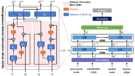
Figure 4: Architecture of the heterogeneous GNN. $h_{t}$ and $h_{c}$ denote the node embedding, $x_{t}$ and $x_{c}$ denote the edge embedding. The subscript letter $l$ represents the $l$-th layer. The subscript letter $t$ represents the tracker and the letter $c$ represents the calorimeter. $\phi_{e}$, $\phi_{x}$, $\phi_{h}$ and $\phi_{g}$ are neural networks of MLPs.

Systematic Uncertainties

Several sources of systematic uncertainties have been carefully evaluated:

1. Uncertainty from Higgs Boson Count: The uncertainty originating from the total number of Higgs bosons is estimated to be $1.0\%$ [40]. This accounts for variations in the production rate and experimental measurement of Higgs boson events.

2. Neural Network Training Variability: To assess the robustness of our machine learning model, we trained 50 CNNs with different initial seeds. The training uncertainty for the neural networks is estimated as half of the difference between the maximum and minimum efficiencies observed, which amounts to approximately $1.7\%$.

A quadratic sum of the above two uncertainties yields a total systematic uncertainty of $2.0\%$.

III Results

To fully explore the potential of searching for LLPs with lepton colliders, we develop a novel approach that directly utilizes the low-level detector information based on the energy, position, and time of detector hits, in contrast to the traditional approach which performs a full event reconstruction. Detailed information on the general analysis strategy and the deep learning networks used in this work is described in the ”Methods” section and ”Supplementary Information”. Fig. 2 shows the structure of the Convolutional Neural Networks model [22], and Fig. 4 illustrates the architecture of the Graph Neural Networks [23]. Both CNN and GNN methods have been evaluated for the efficiency of LLPs signals (type I and II signals combined) while keeping background free, the efficiency results are summarized in Table 2. The signal efficiencies of the CNN method range from 74% to 99%, while the GNN method efficiencies range from 79% to 97% for various LLP masses and lifetimes. Both efficiency numbers are similar. We calculate the signal acceptance based on CEPC detector geometry settings with the full detector coverage [24]. The signal acceptance factors are summarized in Table 3. We then multiply the signal efficiency by the signal acceptance to obtain the signal yield. The signal yield is shown in Figure 5.

Table 2: Signal efficiencies for different LLPs masses and lifetimes obtained with CNN-based and GNN-based approaches. All efficiency values are presented with their corresponding statistical uncertainties.

Approach	Efficiency (%)	Lifetime [ns]
	Mass [GeV]	0.001	0.1	1	10	100
CNN	1	$81.8\pm 0.1$	$90.7\pm 0.1$	$78.9\pm 0.2$	$74.4\pm 0.6$	$76.5\pm 1.9$
	10	$80.2\pm 0.1$	$89.5\pm 0.1$	$91.2\pm 0.1$	$88.7\pm 0.1$	$83.6\pm 0.5$
	50	$87.5\pm 0.1$	$96.7\pm 0.1$	$99.3\pm 0.0$	$98.4\pm 0.0$	$93.5\pm 0.1$
GNN	1	$82.9\pm 0.1$	$89.4\pm 0.1$	$79.9\pm 0.2$	$79.9\pm 0.6$	$80.2\pm 1.8$
	10	$76.7\pm 0.1$	$86.0\pm 0.1$	$91.2\pm 0.1$	$85.7\pm 0.2$	$83.7\pm 0.5$
	50	$88.0\pm 0.1$	$91.8\pm 0.1$	$97.4\pm 0.1$	$97.4\pm 0.1$	$93.0\pm 0.1$

Table 3: Signal acceptances for different LLPs masses and lifetimes, including statistical uncertainties.

Acceptance (%)	Lifetime [ns]
Mass [GeV]	0.001	0.1	1	10	100
1	100.00 $\pm$ 0.00	99.86 $\pm$ 0.01	48.76 $\pm$ 0.18	6.49 $\pm$ 0.09	0.67 $\pm$ 0.03
10	100.00 $\pm$ 0.00	100.00 $\pm$ 0.00	99.78 $\pm$ 0.01	46.80 $\pm$ 0.16	6.22 $\pm$ 0.08
50	100.00 $\pm$ 0.00	100.00 $\pm$ 0.00	100.00 $\pm$ 0.00	99.31 $\pm$ 0.03	40.37 $\pm$ 0.16

Figure 5: Efficiency and acceptance of LLP Detection. The product of geometry acceptance and selection efficiency for LLPs with varying masses and lifetimes. Solid symbols represent data from a CNN-based approach, while hollow symbols are from a GNN-based approach. The varied shapes correspond to different assumed LLP masses, with circles for 50 GeV, diamonds for 10 GeV, and crosses for 1 GeV. The error bars representing statistical uncertainties have been omitted from the figure as their values are too small for effective visual representation.

To estimate the sensitivity of the study, we assume a null hypothesis for LLPs signals and obtain 95% Confidence Level upper limits [41] on the branching ratio $\mathcal{B}(H\rightarrow\text{LLPs})$ for the process $e^{+}e^{-}\to ZH(Z\to\text{inclusive},H\to X_{1}+X_{2}$). The analyzed samples have a $20\text{~{}ab}^{-1}$ luminosity and about $4\times 10^{6}$ Higgs bosons. For the two LLPs signal types, we have considered the following scenarios:

• Type I and Type II signal yields have a fixed ratio. We define a parameter $\epsilon_{V}:=\frac{BR(X\to\nu\bar{\nu})}{BR(X\to q\bar{q})}$ as the ratio and set it with a fixed value of 0.2. A one-dimensional 95% Confidence Level upper limit on $\mathcal{B}(H\rightarrow\text{LLPs})$ is derived and shown in Figure 6a).

• Type I and Type II signal yields have a floating ratio $\epsilon_{V}$ with an allowed range of $10^{-6}$ and $100$. A one-dimensional 95% Confidence Level upper limit on $\mathcal{B}(H\rightarrow\text{LLPs})$ is derived and shown in Figure 6b).

• Type I and Type II signal yields has a floating ratio and two-dimensional 95% Confidence Level upper limits on $\mathcal{B}_{\text{2-jet}}$ and $\mathcal{B}_{\text{4-jet}}$ are derived. A bivariate statistical fit is performed to derive the upper limits and results are shown in Figure 7. More detailed results on 2-D upper limits can be found in Sec. 1.4 in ”Supplementary Information”.

Both 1-D and 2-D exclusion limits are summarized in Table 4. As the results indicate, statistical uncertainties dominate in this analysis. For systematic uncertainties, refer to the ’Systematic Uncertainty’ section.

(a)

(b)

Figure 6: One-dimensional constraints on Higgs boson decay to LLPs. 95% C.L. upper limit on the branching ratio (BR) for the Higgs boson ($H$) decay into pairs of LLPs ($X_{1}X_{2}$) via $e^{+}e^{-}\to ZH$, where $\epsilon_{V}$ is the ratio $\frac{BR(X\to\nu\bar{\nu})}{BR(X\to q\bar{q})}$. a): a fixed ratio $\epsilon_{V}=0.2$, b): a floating $\epsilon_{V}$. The shaded areas indicate statistical and systematic uncertainties combined.

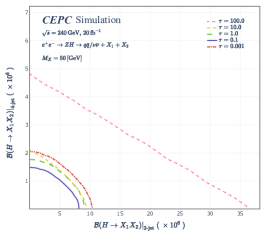
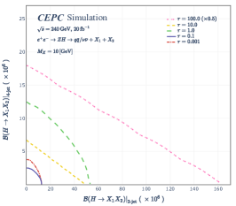
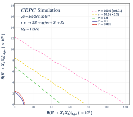
Figure 7: Two-dimensional constraints on Higgs Boson decay to LLPs. The 95% C.L. 2-D upper limit on ($\mathcal{B}_{\textrm{2-jet}}$, $\mathcal{B}_{\textrm{4-jet}}$) for the process $e^{+}e^{-}\to ZH$ for three LLPs masses 50 GeV (left), 10 GeV (middle), 1 GeV (right). Different colored lines indicate different LLPs lifetimes. The uncertainties on the limits are omitted and a few limits are scaled by a factor for better visibility.

Table 4: The 95% C.L. exclusion limit on BR($h\to X_{1}X_{2}$) for all signal channels with both fixed and floating $\epsilon_{V}$. The limits include $\pm 1\sigma$ uncertainties after taking into account both statistical and systematic contributions.

Scenario	$\mathcal{B}$ ($\times 10^{-6}$)	Lifetime [ns]
	Mass [GeV]	0.001	0.1	1	10	100
Fixed	1	$1.9^{+0.5}_{-0.3}$	$1.5^{+0.4}_{-0.2}$	$5.0^{+1.4}_{-0.7}$	$32.4^{+8.0}_{-3.6}$	$933.1^{+237.3}_{-74.4}$
	10	$2.7^{+0.8}_{-0.2}$	$1.9^{+0.6}_{-0.2}$	$2.2^{+0.7}_{-0.3}$	$4.7^{+1.6}_{-0.6}$	$27.6^{+6.0}_{-2.0}$
	50	$1.5^{+0.6}_{-0.1}$	$1.2^{+0.4}_{-0.1}$	$1.4^{+0.3}_{-0.2}$	$1.4^{+0.3}_{-0.2}$	$3.4^{+1.0}_{-0.3}$
Floating	1	$2.7^{+1.1}_{-1.8}$	$1.8^{+1.4}_{-1.0}$	$2.9^{+6.1}_{-0.4}$	$16.4^{+31.0}_{-0.8}$	$493.4^{+1090.1}_{-39.7}$
	10	$3.8^{+0.3}_{-2.5}$	$4.3^{+0.5}_{-3.3}$	$1.3^{+2.7}_{-0.2}$	$2.8^{+5.8}_{-0.4}$	$15.3^{+24.6}_{-2.0}$
	50	$2.8^{+1.0}_{-2.0}$	$2.4^{+0.7}_{-1.8}$	$1.5^{+1.3}_{-0.8}$	$1.5^{+1.3}_{-0.8}$	$2.1^{+4.2}_{-0.2}$

Discussion

We evaluate the effectiveness of our ML-based approach for LLPs detection at future lepton colliders by comparing our results with results at hadron colliders with the ATLAS experiment [13] and CMS experiment [14] as well as future HL-LHC experiments [25]. The comparison is based on four primary metrics: signal acceptance, selection efficiency, analysis strategy and signal yields:

• Signal Acceptance: Both ATLAS and CMS results have limited signal acceptance, typically a few percent, as they focus on LLPs decaying in the muon detector. In contrast, our ML-based approach covers the entire detector, resulting in 100% signal acceptance except for LLPs with long lifetime ($>10$ ns) and low mass ($<10$ GeV).

• Selection Efficiency: For hadron colliders, LLPs events typically trigger on displaced decays and/or large missing transverse energy. The LLPs trigger efficiency at the ATLAS experiment is estimated to be between $10^{-3}$ and $0.3$ [13]. Besides trigger efficiency, there are additional efficiencies involved such as displaced vertex/object reconstruction efficiencies which are typically in the order of a few percent. In contrast, LLPs event selection at lepton colliders can adapt to a triggerless approach owing to the clean environment. ML-based approach can be applied directly with low-level detector information without any event-level reconstruction. As a result, our ML-based approach with lepton colliders can achieve an overall selection efficiency as high as $99\%$, an improvement of several orders in magnitude when comparing with LHC or HL-LHC efficiencies.

• Analysis Strategy: Traditionally, analyses of LLPs conducted elsewhere have employed a selection-based method, which involves categorizing events into multiple subsets with different decay modes and orthogonal signal types. These analyses necessitate manual re-tuning and re-optimization for each subset and different LLPs mass and lifetime configurations. In contrast, our ML-based approach eliminates the need for manual categorization and optimization. Deep neural networks can be retrained with similar setup for each LLPs mass and lifetime, resulting in higher efficiencies compared to the selection-based method. Detailed comparison between two methods is shown in Sec. 1.1 in ”Supplementary Information”.

• Signal Yields and Upper Limits Comparison: LHC and HL-LHC can produce a significantly larger number of Higgs bosons compared to lepton colliders. Despite this, higher signal acceptance and selection efficiencies in our ML-based approach compensate for the relatively low number of Higgs bosons. We achieve upper limits as low as $1.2\times 10^{-6}$ on $\mathcal{B}(H\rightarrow\text{LLPs})$ with $4\times 10^{6}$ Higgs bosons. This upper limit is approximately three orders of magnitude better than the $10^{-3}$ limit observed at the ATLAS and CMS experiments with $10^{7}$ Higgs bosons and it is comparable to the projected HL-LHC limit with about $10^{8}$ expected Higgs bosons.

Besides comparing with hadron colliders, we have also compared our result with a preliminary study [26] on the ILC [27] sensitivity with a traditional selection-based method. The ILC sensitivity study searches for long-lived dark photons produced in Higgstrahlung events via the Higgs portal. We have compared our result with the hadronic decay dark photo result since the event signature is similar. We have seen that the signal acceptance factors are similar between ILC and CEPC detectors but the signal efficiencies differ significantly. The signal efficiencies in the ILC study range from $0.1\%$ to $10\%$, which is at least an order of magnitude lower than ours. The upper limits on $\mathcal{B}(H\rightarrow\text{LLPs})$ in the ILC study are derived under the assumption of $100\%$ truth-level signal efficiency. Under this assumption, two results show similar sensitivities only in the low lifetime region ($<1~{}ns$) of LLPs. In the long lifetime region, for example, for a 1 GeV LLP with a lifetime of a few nanoseconds, our result yields an upper limit of about $5\times 10^{-6}$ which is an order of magnitude better than the ILC’s upper limit of $10^{-4}$.

In summary, we have developed an ML-based approach for LLP searches that outperforms traditional selection-based methods on almost all fronts. Moreover, our ML-based approach can be easily applied to other future lepton collider experiments, including the ILC, FCC [28], and CLIC [29].

There has been recent progress in LLP searches using ML-assisted approaches at hadron colliders [30, 31]. These results utilize ML techniques to perform object-level tagging looking for LLP signatures after full event reconstruction. The tagging performance relies on a limited number of high-level input variables. In our approach, both low-level information (based on hits) and global features of the event have been taken into account. Due to the harsh environment at hadron colliders, controlling the background becomes more challenging, which may require higher granularity and additional input features when constructing the neural networks. Additionally, advanced triggers with fast neural networks are necessary to efficiently capture LLP-like events at hadron colliders [32, 33].

IV Acknowledgement

The authors thank theorists Zhen Liu, Tao Liu, Jia Liu, Ziping Wang, as well as experimentalists Manqi Ruan and Gang Li for their useful suggestions and inputs about the paper. This work was sponsored by the National Key R&D Program of China (2022ZD0117804), National Natural Science Foundation of China (Grants No. 12211540001 and No. 12305217), Key Research Project of Zhejiang Lab (No. 2022PI0AC01), Guangdong Major Project of Basic and Applied Basic Research (No. 2020B0301030008), Science and Technology Program of Guangzhou (No. 2019050001).

Supplementary Information

I.1 A selection-based analysis

Searching for LLPs with the selection-based method is roughly carried out using various reconstruction observable. However, we only investigate a special case that LLPs have long displaced vertices and decay inside the muon detector. In this case, lots of shower hits and an energy burst are expected in the muon detector. Thus, we can save most signal events while almost kicking out all SM background events after applying the following selections,

• $E_{2jets}>$ 30 GeV: the total energy deposition in the muon detector,

• $\Delta T_{j}=\min\left(t_{\text{hit},i}-r_{\text{hit},i}/c\right)\geq 3$ ns: the minimal time difference, where $t_{\text{hit},i}$ represents the hitting time of the $i^{\text{th}}$ component in the jet cluster measured by the muon spectrometer and $r_{\text{hit},i}$ is the $i^{\text{th}}$ Euclidean distance to IP, and c the light speed in vacuum.

• $N_{\textrm{PFOs}}$: number of reconstructed particle flow objects,

• $\not{E}$: the missing energy determined with reconstructed energy in detector subtraction from initial electron-positron c.m. energy.

Table 5 summarizes number of events after imposing a selection chain on both simulated signal and background samples.

Traditional methods generally faces various difficulties in reconstructing and identifying both Z bosons and LLPs, and thus require complicated case-by-case analyses, while the machine learning approach does not. The latter approach uniformly makes use of all available information of event data, and not only exhibits a technical superiority but also systematically improves signal efficiencies, as shown in Table 1 in the paper and Table 5. The signal efficiency is about 97%-98% with a LLP lifetime of 10 ns and mass of 50 GeV, significantly higher than 50.8% obtained with the traditional approach.

Table 5: Number of signal and background events after various selection criteria. MC simulation samples are produced corresponding to the integrated luminosity 5.6 $ab^{-1}$. Signal events have a LLP lifetime of 20 ns and mass of 50 GeV.

Selections	LLPs Signal with $Z\to j\bar{j}$	$ee\to q\bar{q}$	$ee\to ZH$
generated	$1.0\times 10^{6}$	$2.5\times 10^{8}$	$0.99\times 10^{7}$
decay in muon detector	134559	6516657	796596
$|m_{q\bar{q}}-m_{Z}|<15GeV$	113723	4013875	39631
$|m_{q\bar{q}}-m_{H}|<15GeV$	104942	229703	26862
$0.23<y_{12}<0.72$	93,517	129,546	20,041
$E_{2jets}>30\textrm{GeV}$	69,468	72	16
$min(\Delta T_{j_{1}},\Delta T_{j_{2}})>3\textrm{ns}$	68,368	50	11
Efficiency	50.80%	$7.7\times 10^{-6}$	$1.4\times 10^{-5}$

I.2 Searching for LLPs by placing an external detector

We explore the potential of enhancing the discovery sensitivity by placing an external detector far away from the baseline detector. A typical external detector is a stack consisting of multi-layer scintillators. The distance between the outermost and innermost layers is 100 meters. This detector only covers the barrel region, corresponding to an approximated geometry acceptance of 0.65, which allows us to detect LLPs decaying outside the baseline detector from 6 meters to 106 meters. The gain factor is roughly evaluated in accordance with signal efficiency linked to geometry parameters of the external detector,

$$F_{\textrm{gain}}=\frac{N_{\textrm{obs}}}{N_{\textrm{gen}}}=\frac{\Delta\Omega}{4\pi}\frac{\Delta L}{d}e^{-\frac{L}{d}}$$ (2)

where $N_{obs}$ represents the number of observed events among the number of generated events expected, $\Delta\Omega$ represents overall acceptance of external detector among $4\pi$ solid space, $\Delta L$ the longitudinal length of external detector, and d the expected decay length of LLPs in Lab. frame. Table 6 summarizes gain factors compared to the baseline detector. A maximum gain factor of 16.2 can be achieved.

Table 6: The expected gain factor by placing an external detector in detecting LLPs with various masses and lifetimes.

-	$F_{\textrm{gain}}$	Lifetime [ns]
	Mass [GeV]	0.001	0.1	1	10	100
Ext. Detector	1	1	1	3.2	11.6	16.2
	10	1	1	1	3.3	11.8
	50	1	1	1	1.1	3.6

I.3 Training Loss

Figure 8 illustrates values of the loss function variation with the training epochs as training the CNN and GNN. A clear convergence can be seen during training various simulation samples corresponding to LLPs of different masses and lifetimes.

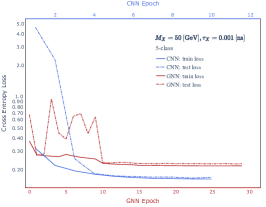
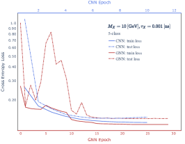
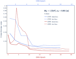
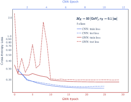
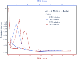
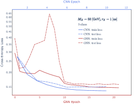
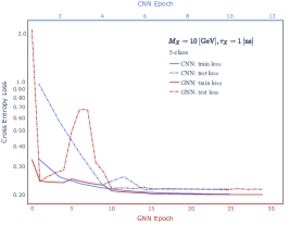
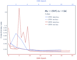
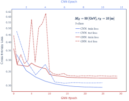
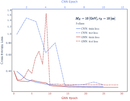
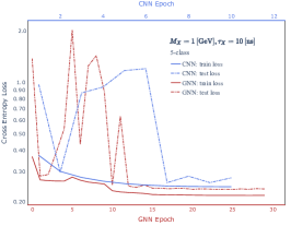
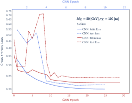
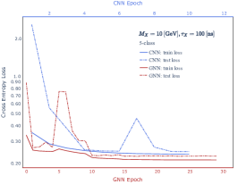
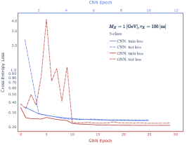
Figure 8: The loss function converges as training epochs increase when training the CNN and GNN. From top to bottom, the LLPs’ lifetime in corresponding samples are 0.001, 0.1, 1, 10, 100 nanoseconds; From left to right, the LLPs’ mass in corresponding samples are 50, 10, 1 GeV.

I.4 Two dimensional upper limits on ($\mathcal{B}_{\textrm{2-jet}}$, $\mathcal{B}_{\textrm{4-jet}}$)

Figure 9 illustrates two dimensional upper limits for LLPs assuming a statistics of $4\times 10^{6}$ Higgs boson.

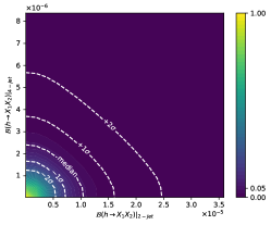
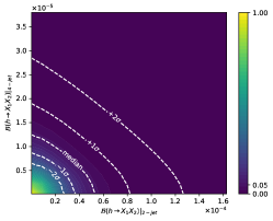
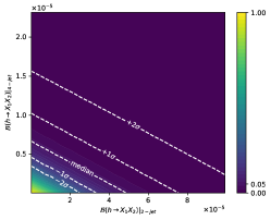
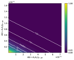
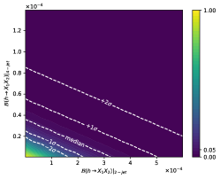
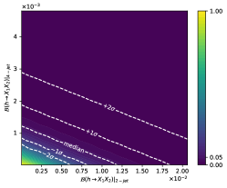
Figure 9: The CLs 2D fitting for ($\mathcal{B}_{\textrm{2-jet}}$, $\mathcal{B}_{\textrm{4-jet}}$). From left to right, the LLP’s mass in corresponding samples are set to 50, 10, 1 GeV; From top to bottom, the LLP’s lifetime are set to 0.0001, 0.1, 1.0, 10, 100 nanoseconds.

References

- [1] The CEPC Study Group. CEPC Conceptual Design Report: Volume 1 - Accelerator. Preprint at arXiv:1809.002855 (2018). https://arxiv.org/abs/1809.00285
- [2] The CEPC Study Group. CEPC Technical Design Report – Accelerator. Preprint at arXiv:2312.14363 (2023). https://doi.org/10.48550/arXiv.2312.14363
- [3] Arvanitaki, A., Craig, N., Dimopoulos, S. & Villadoro, G. Mini-Split. J. High Energ. Phys., 02, 126 (2013). https://doi.org/10.1007/JHEP02(2013)126
- [4] Fan, J., Reece, M. & Ruderman, J. T. Stealth Supersymmetry. J. High Energ. Phys., 11, 012 (2011). https://doi.org/10.1007/JHEP11(2011)012
- [5] Kaplan, D. E., Luty, M. A. & Zurek, K. M. Asymmetric Dark Matter. Phys. Rev. D, 79, 115016 (2009). https://doi.org/10.1103/PhysRevD.79.115016
- [6] Kim, I.-W. & Zurek, K. M. Flavor and Collider Signatures of Asymmetric Dark Matter. Phys. Rev. D, 89, 3, 035008 (2014). https://doi.org/10.1103/PhysRevD.89.035008
- [7] Dienes, K. R. & Thomas, B. Dynamical Dark Matter: I. Theoretical Overview. Phys. Rev. D, 85, 083523 (2012). https://doi.org/10.1103/PhysRevD.85.083523
- [8] Cui, Y. & Shuve, B. Probing Baryogenesis with Displaced Vertices at the LHC. J. High Energ. Phys., 02, 049 (2015). https://doi.org/10.1007/JHEP02(2015)049
- [9] Campbell, B. A., Davidson, S., Ellis, J. R. & Olive, K. A. Cosmological baryon asymmetry constraints on extensions of the standard model. Phys. Lett. B, 256, 484-490 (1991). https://doi.org/10.1016/0370-2693(91)91795-W
- [10] Bouquet, A. & Salati, P. R Parity Breaking and Cosmological Consequences. Nucl. Phys. B, 284, 557 (1987). https://doi.org/10.1016/0550-3213(87)90050-2
- [11] Graesser, M. L. Broadening the Higgs boson with right-handed neutrinos and a higher dimension operator at the electroweak scale. Phys. Rev. D, 76, 075006 (2007). https://doi.org/10.1103/PhysRevD.76.075006
- [12] Maiezza, A., Nemevšek, M., Nesti, F. Lepton Number Violation in Higgs Decay at LHC. Phys. Rev. Lett. 115, 081802 (2015). https://doi.org/10.1103/PhysRevLett.115.081802
- [13] Aad, G., et al. Search for events with a pair of displaced vertices from long-lived neutral particles decaying into hadronic jets in the ATLAS muon spectrometer in collisions at . Phys. Rev. D 106, 3, 032005 (2022). https://doi.org/10.1103/PhysRevD.106.032005
- [14] Tumasyan, A., et al. Search for long-lived particles decaying to a pair of muons in proton-proton collisions at TeV. J. High Energ. Phys., 2023, 5, 228 (2023). https://doi.org/10.1007/JHEP05(2023)228
- [15] Calefice, L., et al. Effect of the high-level trigger for detecting long-lived particles at LHCb. Front. Big Data, 5, 1008737 (2022). https://doi.org/10.3389/fdata.2022.1008737
- [16] Ferber, T., et al. Displaced or invisible? ALPs from decays at Belle II. J. High Energ. Phys., 2023, 4, 131 (2023). https://doi.org/10.1007/JHEP04(2023)131
- [17] Ablikim, M., et al. Search for an axion-like particle in radiative decays. Phys. Lett. B, 838, 137698 (2023). https://doi.org/10.1016/j.physletb.2023.137698
- [18] BaBar Collaboration. Lees, J. P., et al. Search for Long-Lived Particles in Collisions. Phys. Rev. Lett. 114, 171801 (2015). https://doi.org/10.1103/PhysRevLett.114.171801
- [19] Alwall, J., et al. The automated computation of tree-level and next-to-leading order differential cross sections, and their matching to parton shower simulations. J. High Energ. Phys. 07, 079 (2014). https://doi.org/10.1007/JHEP07(2014)079
- [20] Kilian, W., Ohl, T. & Reuter, J. WHIZARD: Simulating Multi-Particle Processes at LHC and ILC. Eur. Phys. J. C 71, 1742 (2011). https://doi.org/10.1140/epjc/s10052-011-1742-y
- [21] Moretti, M., Ohl, T. & Reuter, J. O’Mega: An Optimizing matrix element generator. Preprint at arXiv:0102195 (2001). https://arxiv.org/abs/hep-ph/0102195
- [22] He, K., Zhang, X., Ren, S. & Sun, J. Deep Residual Learning for Image Recognition. Preprint at arXiv:1512.03385 (2015). http://arxiv.org/abs/1512.03385
- [23] Shlomi, J., Battaglia, P. & Vlimant, J.-R. Graph neural networks in particle physics. Mach. Learn. Sci. Technol. 2, 021001 (2020). https://dx.doi.org/10.1088/2632-2153/abbf9a
- [24] The CEPC Study Group. CEPC Conceptual Design Report: Volume 2 - Physics & Detector. Preprint at arXiv:1811.10545 (2018). https://arxiv.org/abs/1811.10545
- [25] Liu, J., Liu, Z. & Wang, L.-T. Enhancing Long-Lived Particles Searches at the LHC with Precision Timing Information. Phys. Rev. Lett. 122, 131801 (2019). https://link.aps.org/doi/10.1103/PhysRevLett.122.131801
- [26] Jeanty, L., Nosler, L. & Potter, C. Sensitivity to decays of long-lived dark photons at the ILC (A Snowmass White Paper). Preprint at arXiv:2203.08347 (2022). https://doi.org/10.48550/arXiv.2203.08347
- [27] Aihara, H., et al. The International Linear Collider. A Global Project. Preprint at arXiv:1901.09829 (2019). https://arxiv.org/abs/1901.09829
- [28] Abada, A., et al. FCC Physics Opportunities: Future Circular Collider Conceptual Design Report Volume 1. Eur. Phys. J. C 79, 474 (2019). https://doi.org/10.1140/epjc/s10052-019-6904-3
- [29] de Blas, J. et al. The CLIC Potential for New Physics. CERN Yellow Reports: Monographs 3, (2018). https://doi.org/10.23731/CYRM-2018-003
- [30] Aad, G. et al. Search for neutral long-lived particles in pp collisions at TeV that decay into displaced hadronic jets in the ATLAS calorimeter. J. High Energ. Phys. 2022, 6, 5 (2022). https://link.springer.com/article/10.1007/JHEP06(2022)005
- [31] The CMS Collaboration. A deep neural network to search for new long-lived particles decaying to jets. Mach. Learn.: Sci. Technol. 1, 3, 035012 (2020). https://iopscience.iop.org/article/10.1088/2632-2153/ab9023
- [32] Alimena, J., Iiyama, Y. & Kieseler, J. Fast convolutional neural networks for identifying long-lived particles in a high-granularity calorimeter. J. Instrum. 15, 12, P12006 (2020). https://doi.org/10.1088/1748-0221/15/12/P12006
- [33] Coccaro, A., Di Bello, F. A., Giagu, S., Rambelli, L. & Stocchetti, N. Fast neural network inference on FPGAs for triggering on long-lived particles at colliders. Mach. Learn.: Sci. Technol. 4, 4, 045040 (2023). https://iopscience.iop.org/article/10.1088/2632-2153/ad087a
- [34] Mora de Freitas, P. & Videau, H. Detector simulation with MOKKA / GEANT4: Present and future. International Workshop on Linear Colliders (LCWS 2002), 623-627 (2002). http://inspirehep.net/record/609687
- [35] Aplin, S. J., Engels, J. & Gaede, F. A production system for massive data processing in ILCSoft. EUDET-MEMO-2009-12 (2009). https://inspirehep.net/literature/889841
- [36] Chen, T. & Guestrin, C. XGBoost: A Scalable Tree Boosting System. Preprint at arXiv:1603.02754 (2016). http://dx.doi.org/10.1145/2939672.2939785
- [37] Wilks, S. S. The Large-Sample Distribution of the Likelihood Ratio for Testing Composite Hypotheses. Ann. Math. Stat. 9, 60-62 (1938). http://www.jstor.org/stable/2957648
- [38] Gong, S., et al. An efficient Lorentz equivariant graph neural network for jet tagging. J. High Energ. Phys. 2022, 7, 030 (2022). https://doi.org/10.1007/JHEP07(2022)030
- [39] Satorras, V. G., Hoogeboom, E. & Welling, M. E (n) equivariant graph neural networks. Proc. 38th Int. Conf. Mach. Learn. 139, 9323-9332 (PMLR, 2021). https://proceedings.mlr.press/v139/satorras21a.html
- [40] Smiljanic, I., et al. Systematic uncertainties in integrated luminosity measurement at CEPC. Preprint at arXiv:2010.15061 (2020). http://arxiv.org/abs/2010.15061
- [41] Read, A. L. Modified frequentist analysis of search results (the method). CERN Open Archive CERN-OPEN-2000-205 (2000). https://cds.cern.ch/record/451614
- [42] The total invisible decay of LLPs (type III signal) is not considered in this analysis.
- [43] Detectable means that LLPs have visible decay products within the geometric acceptance of the detector.