Universal Statistics of Competition in Democratic Elections

Abstract

Elections for public offices in democratic nations are large-scale examples of collective human behavior. As a statistical physics problem with complex interactions among agents, we can anticipate that universal macroscopic patterns can emerge independent of microscopic details. Despite the availability of empirical election data, such universality, valid at all scales, countries, and elections, has not yet been observed. In contrast to all previous attempts in this direction, in this work, it is shown that the distribution of vote margins is driven by that of voter turnout. We use empirical data from $34$ countries to demonstrate that a scaled measure depending on margin and turnout leads to robust universality. Further, a voting model is introduced, which reproduces all the observed universal features. The deviations from universality indicate possible electoral malpractices. We argue that the universality is a stylized fact indicating the competitive nature of electoral outcomes.

One of the cornerstones of democratic societies is that governance must be based on an expression of the collective will of the citizens. The institution of elections is central to the operational success of this system. Elections to public offices are the best-documented instances of collective decision-making by humans, whose outcome is determined by multiple agents interacting over a range of spatial and temporal scales. These features make elections an interesting test-bed for statistical physics whose key lesson is that a multitude of complex interactions between microscopic units of a system can manifest into robust, universal behavior at a macroscopic level [1, 2, 3, 4, 5, 6, 7, 8, 9, 10, 11, 12, 13]. A collection of gas molecules or spins are examples that display such emergent macroscopic features [14], and so do complex processes such as earthquakes [15, 16], financial markets [17] and stationary dynamics on networks [18]. In the context of elections, universality serves to distill the complexities of electoral dynamics into understandable and predictive frameworks and safeguard its integrity.

Unsurprisingly, the possibility of universality attracts significant research attention [19, 20, 21, 22, 23, 24, 25]. Several works have studied and proposed models for (a) the distribution $f(v)$ of the fraction of votes $v$ obtained by candidates (or the vote share), and (b) distribution $g(\tau)$ of voter turnout $\tau$. While $v$ is indicative of popularity, $\tau$ indicates the scale of the election. Though some universality has been observed in $f(v)$ or $g(\tau)$ within a single country [20, 19, 21] or in countries with similar election protocols [20, 24], deviations from claimed universalities have also been reported [24, 26, 27, 28, 29] due to variations in the size (scale) of electoral districts and weak party associations. Though voting patterns tend to display spatial correlations [30, 31, 32, 33], it is not known to be universal. Despite the availability of enormous election data and persistent attempts, a robust and universal emergent behavior, valid across different scales and countries with vastly different election protocols, is yet to be demonstrated.

In this Letter, using extensive election data [34, 35, 36, 37] from 34 countries (from 6 continents) spanning multiple decades and electorate scales, we demonstrate universality through analysis of the margin of victory and turnout data in democratic elections. The margin of victory (or simply the margin) is a key indicator of competition in elections and a proxy for the healthy functioning of democracies. While the turnout data has been studied in various settings, margins have never been considered in the context of universality. We introduce a Random Voting Model (RVM) to demonstrate that turnout distribution drives the distribution of scaled margins. With this insight, we show that the scaled margin-to-turnout ratio distribution has a universal form valid for all democratic elections across countries at different scales. The RVM captures this universality, which, along with the prediction for scaled margin distribution, is useful for flagging electoral malpractice as well. Several studies [38, 39], correlating turnout to winner voteshare, have found markers for flagging potential misconduct.

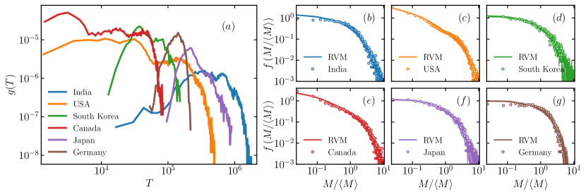
Figure 1: (a) Turnout distribution $g(T)$ obtained from election data for different countries. Note the wide differences in shapes and ranges for $g(T)$. (b-g) Rescaled margin distribution $f(M/\langle M\rangle)$ obtained from election data (open circles) and the model predictions (solid lines). An excellent agreement is observed between the empirical data and model-generated distributions. The lighter shade around the model prediction (solid line) represents its variability estimated from multiple RVM realizations.

A template of a basic electoral process is as follows. At each electoral unit, candidates compete against each other to win the votes of the electorate, who can cast their vote in favor of only one of the candidates. The candidate securing the largest number of polled votes is declared the winner. This represents the core process in many electoral systems. It is the standard first-past-the-post system followed in many countries, e.g., India, the UK, and the USA. In an instant-run-off system (such as in Australia) or two-round run-offs (such as in France), the final run-off round boils down to this template. Typically, national or regional elections following this template consist of many electoral units made up of polling booths, precincts, constituencies, and counties. These units set a size scale in terms of the number of electorates – polling booth represents the smallest scale, while a constituency (subsuming many polling booths) represents the largest scale. For our analysis, an “election” could be either a national, regional, or even a city-level electoral process encompassing $N$ electoral units, and each unit could be a polling booth, county, or constituency.

In any such election, an informative indicator of the degree of competition and the extent of consensus is the margin. A vanishing margin signifies tight competition and a divided electorate, whereas large margins indicate a decisive mandate and overwhelming consensus in favor of one candidate. Let $c_{i},i=1,2,\dots N$ denote the number of candidates contesting an election in $N$ distinct electoral units. The winning and runner-up candidates receive, respectively, $v_{w,i}$ and $v_{r,i}$ votes such that $v_{w,i}>v_{r,i}$. The margin is given by $M_{i}=v_{w,i}-v_{r,i}$. If $n_{i}>0$ is the size of the electorate, i.e., number of registered voters in $i$-th unit, then $0\leq M_{i}\leq n_{i}$. However, in practice, only a fraction of the electorate participates in voting. In such cases, the number of voters who show up to cast their vote is termed as the turnout $T_{i}$, such that $0\leq T_{i}\leq n_{i}$, and consequently, the margin is further restricted by $0\leq M_{i}\leq T_{i}$. By rescaling with $T_{i}$, we get

$$0\leq\frac{M_{i}}{T_{i}}\leq 1.$$ (1)

This provides the first key hint that the ratio $\mu=M/T$, referred to as the specific margin, might be a relevant object of interest as it provides a measure of competitiveness, irrespective of the size of the electoral unit.

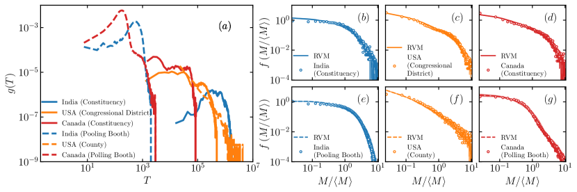
Figure 2: The turnout and rescaled margin distribution for India (blue), the USA (orange), and Canada (red), at two widely different scales, i.e., size of electoral units. (a) Turnout distribution $g(T)$ at two different scales for each country. The dashed line is for $g(T)$ at a smaller scale (polling booth for India and Canada, County for the USA), and the solid line represents a larger scale (constituency for India and Canada, congressional district for the USA). (b-g) Rescaled margin distribution obtained from election data (open circles) and as predicted by the Random Voting Model (line). Despite the differences in scale and shape of $g(T)$, empirical scaled margin distribution is well described by the Random Voting Model. The lighter shade around the model prediction curves represents its variability estimated from multiple realizations of RVM.

To fix our ideas, we might focus on the elections in one country, e.g., the general elections in India. Then, the object of interest would be $M_{i}$ and $T_{i}$ ($i=1,2,\dots N$). To be statistically robust, the data is consolidated from many elections spread over several decades (For India, $18$ elections from 1951 to 2019; See supplemental Material [40]). This leads to the associated empirical distributions $f(M)$ and $g(T)$, respectively, for margin and turnout. Figure 1(a) displays the distribution of raw turnout $g(T)$ at the constituency level for national elections in six countries, namely, India, USA, South Korea, Canada, Japan, and Germany. Striking dissimilarities in $g(T)$ are visible in the shape and support of distribution for countries. For Germany, $g(T)$ has a unimodal character, while that for Canada and the USA display multiple peaks. The corresponding scaled margin $M/\langle M\rangle$ is displayed as distribution $f(M/\langle M\rangle)$ (computed from the consolidated margin data for each country) in Fig. 1(b-g). They are noticeably distinct for different countries. While $f(M/\langle M\rangle)$ for German elections in Fig. 1(g) has a sharp cutoff, that for India and Japan in Fig. 1(b,f) has a slower decay. These observations motivate the question if the rescaled margin distribution is related to, and if they are obtainable from, the distributions of raw turnout.

To investigate this question, we propose a Random Voting Model (RVM) ${\mathcal{V}}(T)$ that takes raw turnouts $T=\{T_{1},T_{2}\dots T_{N}\}$ as input. This model emulates an election taking place at $N$ electoral units (say, constituencies). At $i$-th unit, each of the $T_{i}$ voters (raw turnout at $i$-th unit) can cast only one vote, independently and by randomly choosing one of the $c_{i}$ contesting candidates. The probability that candidate $j$ in $i$-th unit can attract a vote is $p_{ij}=w_{ij}/\sum_{j}w_{ij}$, where $w_{ij}\in[0,1]$ is a random number drawn from a uniform distribution. Irrespective of number of contesting candidates, most nations effectively have a two-party system, i.e., $v_{w,i}$ and $v_{r,i}$ are the only relevant vote shares. In election data that we use, averaged over all the 34 countries, the top two (three) candidates account for 79% (87%) of all votes polled. Hence, the model assumes three candidates at every constituency: $c_{i}=3$ for $i=1,2\dots N$, and that all eligible voters cast their votes, implying $T_{i}=n_{i}$. By simulating this model, margin $M_{i}$ is obtained for $i$-th electoral unit and $\langle M\rangle=(1/N)\sum_{i=1}^{N}M_{i}$ is the associated sample mean. For a detailed description of the model, see supplemental material [40]. The model predictions depend exclusively on the actual turnout distribution, and no free parameters to be tuned. As illustrated in Fig. 1(b-g), the scaled margin distributions predicted by this model (solid lines in Fig. 1) show a remarkable agreement with those computed from empirical margin data from real elections. Notably, RVM faithfully captures disparate decay features in $f(M/\langle M\rangle)$ for India, USA, South Korea, Canada, Japan, and Germany (for 28 other countries, see supplemental material [40]). This suggests that the raw turnout data carries intrinsic information about the margin distribution. RVM effectively leverages this information embedded in the turnout distribution to predict the scaled margin distribution.

Next, we show that these results are independent of the number of voters or size of electoral units. In large countries, depending on the size of the electoral unit, the typical turnout can differ by several orders of magnitude. For example, in India, polling booths have a typical electoral size $\sim 10^{3}$, whereas, at the parliamentary constituency level, it is about $10^{6}$. Further, the shapes of $g(T)$ are also vastly different at different scales. Figure 2(a) captures the striking differences in range and shape of $g(T)$ for India, the US, and Canada at two different scales. Quite remarkably, despite these vast differences in the scale, the same RVM ${\mathcal{V}}(T)$, without any parameter adjustments, accurately predicts the scaled margin distribution. Figure 2(b,c,d) shows the empirical distribution of scaled margins (in national elections) at the constituency-level scale, and Figure 2(e,f,g) shows the same at the scale of polling booths (county for USA). At both these scales, the margin distribution computed from the model displays a good agreement with the empirical distribution. In particular, for the USA (Fig. 2(c,f)), the county-level distribution shows a heavy-tailed decay but decays faster at the congressional district level. For Canada as well, the empirical scaled margin distributions are noticeably different at two different scales. Yet, all the differences are well captured by the RVM simulations shown as dashed lines in Fig. 2(b-g). Taken together, these results show that the scaled margin distribution depends on the raw turnout distribution, and RVM captures this relation across various countries and at all scales.

Given the suggestive scale-independent turnout-margin connections expressed in Figs. 1 and 2, it can be anticipated that the distribution of specific margin $\mu_{i}=\frac{M_{i}}{T_{i}}$, after suitable rescaling, might display universality. Indeed, we observe a compelling universal behavior in the distribution $F(\mu/\langle\mu\rangle)$, as the empirical data for all the $32$ countries, at different scales and for elections held over a time span of several decades, collapses onto a single universal curve. Figure 3 portrays the universality of $F(\mu/\langle\mu\rangle)$ (shown as solid circles) observed in the empirical election data from $32$ countries. In this, each color of a solid circle represents $F(\mu/\langle\mu\rangle)$ computed from data consolidated over several elections from a particular country. The mean behavior of empirical data is computed by averaging over empirical distributions for all the $32$ countries, and this is shown as red open circles in Fig. 3. The average prediction from RVM (black line) also displays an excellent agreement with the mean empirical distribution (red open circles).

Remarkably, the universality result does not depend on the precise functional form of $g(T)$. With this insight, we assume constant turnout, i.e, $T_{1}=T_{2}=\dots T_{N}=t$, and two candidates in each constituency with equal probability of receiving votes. We designate this as simplified RVM ($s$-RVM). In the limit of large turnout, $T\gg 1$, as shown in the supplemental material [40], we obtain an approximate scaling form

$$F(x)=\mathcal{N}e^{-x^{2}/\pi},\;\;\;\;x=\frac{\mu}{\langle\mu\rangle}>0,$$ (2)

where $\mathcal{N}$ is the normalization constant. This, shown in Fig. 3 as the blue line, is in good agreement with empirical data. This universality suggests that irrespective of the finer details of election processes, the mechanism underlying the core component of any competitive election – choosing one candidate from many contenders – has a statistical description in terms of a time-independent probability distribution for the scaled specific margin $\mu/\langle\mu\rangle$. The RVM describes this universality.

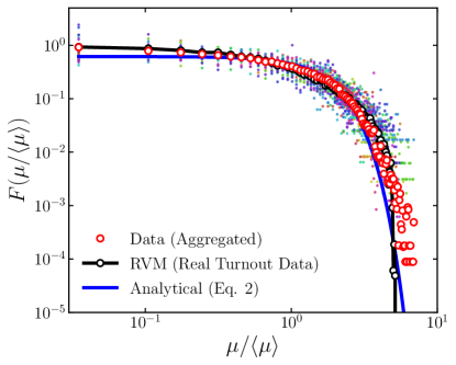
Figure 3: The empirical distribution of $\mu/\langle\mu\rangle$ using data of 32 countries (excluding Ethiopia and Belarus). Each color of the dot corresponds to a specific country, for which the data is consolidated over several elections. The red circles correspond to the average of all the empirical distributions obtained for each country. The prediction from RVM (black line with open circles) closely follows the averaged empirical distribution (red circles). The blue solid line is the analytical prediction of universal scaling from $s$-RVM in Eq. 2.

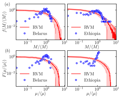
Figure 4: (a) The distribution of scaled margin $f(M/\langle M\rangle)$ using empirical data from Belarus $(2004-2019)$ and Ethiopia $(2010)$(blue circles), compared with model predictions (red line). (b) The distribution of scaled specific margin, $F(\mu/\langle\mu\rangle)$, obtained from empirical data (solid circle), shows significant deviation from the model predictions (red line). The light red shaded region represents the variability in model prediction computed from 100 realizations of the model simulation.

From the robustness of the universality result (Fig. 3) across different countries with a track record of fair election processes, it is reasonable to assume that any pronounced deviation from universality might indicate a prevalence of unfair means in the election process. We search for such deviations in countries with at least $400$ data points in the constituency-level election data. We find that $F(\mu/\langle\mu\rangle)$ computed from data for Ethiopian election of $2010$ and Belarus elections during $2004-2019$ display pronounced deviations from the RVM predictions and universality as seen in Fig. 4(b). Similarly, the empirical scaled margin distribution $f(M/\langle M\rangle)$ deviates significantly from the RVM prediction (Fig. 4(a)). This analysis in Fig. 4 strengthens the skepticism expressed in earlier studies and independent investigations about elections in Ethiopia [41] and Belarus [42, 43, 44, 45]. Electoral malpractices take various forms, and statistical analysis is useful as a prima facie indicator requiring detailed scrutiny. Thus, the robust universality and RVM provide an effective toolbox to flag potentially suspicious elections. We propose that the universality in Fig. 3 should be treated as a stylized fact of elections, which all election models should be able to reproduce.

In summary, competitiveness in any election is encoded in the victory margins and turnouts. The latter also expresses people’s interest in the participatory democratic process. In this work, using extensive empirical election data from $34$ countries, we have obtained two significant results: (a) scaled margin distribution can be predicted from the raw election turnout alone, (b) the scaled distribution of margin-to-turnout ratio $\mu$ has a universal form for all elections independent of country, regions, turnouts and the scale of elections. A parameter-free Random Voting Model introduced in this work faithfully reproduces all these features observed in empirical election data. Both these results can be regarded as stylized facts of elections. Hence, every successful election model, irrespective of its underlying principle and mechanism, must necessarily reproduce these stylized facts to be consistent with real elections. Further, the deviations from the universal scaling function could potentially help in assessing the credibility of the election process. We demonstrate this by flagging the elections of two countries for possible electoral misconduct. This work can be extended to incorporate political party and candidate information, leading to data-driven models with predictive power over the election outcomes.

S1 Supplemental Material for “Universal Statistics of Competition in Democratic Elections”

S1.1 Random Voting Model: Description

We describe a model of election, designated as the Random Voting Model (RVM), in which $c_{i}$ candidates contest at $i$-th electoral unit with $n_{i}$ electors (voters). For each candidate, a number between zero and one is drawn uniformly at random, which is assigned as an unnormalized probability weight $w_{ij}$ to that candidate. The weights are further normalized to get the probability $p_{ij},j=1,2\dots c_{i}$ of receiving votes from the electors. This can be mathematically stated as

$$w_{ij}\sim\mathcal{U}(0,1)\quad\text{and}\quad p_{ij}=\frac{w_{ij}}{\sum_{j}w_{ij}},$$ (S1)

where $\mathcal{U}(0,1)$ is uniformly distributed random numbers in $(0,1)$.

In an election, if there are $n_{i}$ electors (voters) in $i$-th electoral unit, each elector votes for candidate $j$ independently with probability $p_{ij}$. Every voter votes exactly once. The candidate receiving the most votes $v_{w,i}$ is declared the winner, and the candidate securing the next largest number of votes $v_{r,i}$ is the runner-up. The margin of victory $M$ is defined to be the vote difference between the winner and the runner-up: i.e. $M=v_{w,i}-v_{r,i}$. The empirical election data we employ (from 34 countries) shows that the top three candidates, on average, account for nearly 87% of all votes polled in an election. Hence, as part of the model specification, we fix the number of candidates in each electoral unit to be three, i.e., $c_{i}=3$.

The only input to this model is the raw turnout data, i.e., the number of voters (who actually voted) in each constituency. For the model simulation, we use the turnout data of real elections as the total number of voters in different constituencies. To understand how simulations are performed, consider this notional example: if a country has $N=100$ constituencies and data for five such elections is available. Then, the model is simulated on $500$ electoral units. The number of electors in each electoral unit is taken from the consolidated turnouts. Such a simulation of election is performed multiple times to get the average distributions for scaled margins $f(M/\langle M\rangle)$ and scaled specific margins $F(\mu/\langle\mu\rangle)$.

S1.2 Theoretical calculations using $s$-RVM model

To analytically calculate an approximate scaling formula for the distribution of $\mu=\frac{M}{T}$, we further simplify the model by making two simplifying assumptions. We designate this model as $s$-RVM. Firstly, we assume a constant turnout in each electoral unit: $T_{i}=T$ for all $i=1,2,\dots N$. This effectively assumes a constant turnout distribution. This is a reasonable assumption since our empirical analysis of election data indicates that the universality is robust irrespective of the turnout distribution. Further, we assume that two candidates compete in each electoral unit, and the probability of receiving votes is equal for both candidates. In this simplified Random Voting Model ($s$-RVM), the distribution of margin $M$ has the following form:

$$P(M;T)=2^{-T+1}\binom{T}{\frac{T+M}{2}},\;\;\;\;\>0<M\leq T,$$ (S2)

where the quantity within brackets is the Binomial coefficient. As the turnout $T$ is constant, the scaled margin-to-turnout ratio, $x=\mu/\langle\mu\rangle$, is the same as the scaled margin $M/\langle M\rangle$. Hence, $F(x)$ can be calculated through a change of variable as follows:

$$F(x;T)=\langle M\rangle~{}P\left(\langle M\rangle x\right).$$ (S3)

Using Eq. S2, we find the mean margin to be $\langle M\rangle=\sqrt{\frac{2T}{\pi}}$. Using this, we obtain

$$F(x;T)=2^{-T+1}\sqrt{\frac{2T}{\pi}}\binom{T}{\frac{T+x\sqrt{2T/\pi}}{2}}.$$ (S4)

Using Stirling approximation for factorial functions and taking the limit $T\to\infty$, we find half Gaussian as the universal scaling form for $F(x)$ :

$$F(x)=\mathcal{N}e^{-x^{2}/\pi},\;\;\;\;x>0,$$ (S5)

where $\mathcal{N}$ is the normalization constant. This approximate scaling form has a good agreement with the empirical distributions shown in Fig. 3.

S1.3 Data collection and cleaning

In this work, we use empirical election data from 34 countries. Of these, data from 32 countries are used for establishing the universality result, and data from two countries are used to illustrate pronounced cases of deviations from universality.

Data collection– We collect constituency level data of the lower chamber of the Legislative elections for 180 countries and territories across the world from the Constituency-Level Election Archive (CLEA) website [34]. Polling booth level data for India and Canada is collected from the websites of Election Commission [36, 37] of the respective countries, semi-automatically using a combination of Python libraries. For the USA, we collect county level data from MIT Election Data + Science Lab [35]. While constituency level data is available for many countries, polling booth level data is available in the public domain only for a few countries.

Data cleaning–While constituency level data collected from the CLEA website was in tabular format, the polling booth level data was found in different formats, ranging from tabular to machine-generated and scanned PDFs. We clean the data using a combination of Python libraries. Our analysis has been performed on the election data of each country consolidated over several elections. To ensure a reasonable level of confidence in the statistical analysis, we have ignored data from countries that have less than 400 data points. By this criteria, we could use the data from $34$ out of $180$ countries, all of which have more than $400$ data points. The threshold of $400$ data points allows us to demonstrate universality, along with flagging possible electoral misconduct in Ethiopia and Belarus, while maintaining good statistics.

In this analysis, we discard those rare cases when the turnout is zero, or the number of contesting candidates is less than two. To avoid discrepancies, we consider the sum of valid votes received by all the candidates (in an electoral unit) as the turnout for the election in that unit. Some important summary statistics of the election data for the $34$ countries used for analysis in this work are given in table S1.

Country	Time Span	Number of Elections	Scale	Mean Turnout	Mean Margin
Australia	1901-2016	37	Constituency	$7.368\times 10^{4}$	$1.312\times 10^{4}$
Bangladesh	1973-2008	4	Constituency	$1.566\times 10^{5}$	$3.145\times 10^{4}$
Belarus	2004-2019	5	Constituency	$4.830\times 10^{4}$	$2.607\times 10^{4}$
Canada	1867-2019	43	Constituency	$2.765\times 10^{4}$	$5.502\times 10^{3}$
Canada	2004-2021	7	Polling Booth	$5.555\times 10^{2}$	$1.353\times 10^{2}$
Chile	1945-2017	7	Constituency	$1.069\times 10^{5}$	$1.046\times 10^{4}$
Denmark	1849-2019	30	Constituency	$2.697\times 10^{3}$	$4.637\times 10^{2}$
Ethiopia	2010	1	Constituency	$4.952\times 10^{4}$	$4.180\times 10^{4}$
France	1973-2017	3	Constituency	$7.879\times 10^{4}$	$1.096\times 10^{4}$
Germany	1871-2017	19	Constituency	$1.367\times 10^{5}$	$2.257\times 10^{4}$
Ghana	1992-2016	6	Constituency	$3.748\times 10^{4}$	$9.877\times 10^{3}$
Hungary	1990-2018	6	Constituency	$5.323\times 10^{4}$	$8.574\times 10^{3}$
India	1951-2019	18	Constituency	$5.686\times 10^{5}$	$8.333\times 10^{4}$
India	2004-2019	4	Polling Booth	$5.825\times 10^{2}$	$1.891\times 10^{2}$
Japan	1947-2017	26	Constituency	$2.881\times 10^{5}$	$2.351\times 10^{4}$
Kenya	1961-2013	2	Constituency	$3.724\times 10^{4}$	$1.187\times 10^{4}$
Lithuania	1992-2020	8	Constituency	$3.243\times 10^{4}$	$3.980\times 10^{3}$
Malawi	1994-2019	4	Constituency	$2.308\times 10^{4}$	$6.292\times 10^{3}$
Malaysia	1959-2018	13	Constituency	$3.415\times 10^{4}$	$8.900\times 10^{3}$
Myanmar	2010-2015	2	Constituency	$6.757\times 10^{4}$	$2.318\times 10^{4}$
New Zealand	1943-2020	9	Constituency	$3.045\times 10^{4}$	$6.936\times 10^{3}$
Nigeria	2003-2019	2	Constituency	$7.745\times 10^{4}$	$2.202\times 10^{4}$
Pakistan	1988-2013	3	Constituency	$1.278\times 10^{5}$	$2.454\times 10^{4}$
Papua New Guinea	1972-2017	8	Constituency	$5.073\times 10^{4}$	$5.662\times 10^{3}$
Philippines	1946-2013	17	Constituency	$1.830\times 10^{5}$	$2.632\times 10^{4}$
Solomon Islands	1967-2019	14	Constituency	$3.671\times 10^{3}$	$4.373\times 10^{2}$
South Korea	1948-2012	13	Constituency	$6.175\times 10^{4}$	$1.010\times 10^{4}$
Taiwan	1986-2020	11	Constituency	$2.335\times 10^{5}$	$1.976\times 10^{4}$
Tanzania	2005-2020	2	Constituency	$5.366\times 10^{4}$	$2.007\times 10^{4}$
Thailand	1969-2011	12	Constituency	$1.855\times 10^{5}$	$1.464\times 10^{4}$
Trinidad and Tobago	1925-2020	13	Constituency	$1.534\times 10^{4}$	$5.118\times 10^{3}$
Uganda	2006-2021	4	Constituency	$4.453\times 10^{4}$	$1.081\times 10^{4}$
UK	1832-2019	46	Constituency	$3.430\times 10^{4}$	$6.301\times 10^{3}$
Ukraine	1998-2019	5	Constituency	$8.889\times 10^{4}$	$1.670\times 10^{4}$
United States	1788-2020	167	Congressional District	$1.143\times 10^{5}$	$2.958\times 10^{4}$
United States	2000-2020	6	County	$7.048\times 10^{4}$	$1.547\times 10^{4}$
Zimbabwe	2005-2018	4	Constituency	$1.767\times 10^{4}$	$6.554\times 10^{3}$

Table S1: Typical values of Margin and turnouts at different scales for different countries. The available data for the mentioned time spans were consolidated for each country and used to calculate the average. Only national level elections are considered in this dataset.

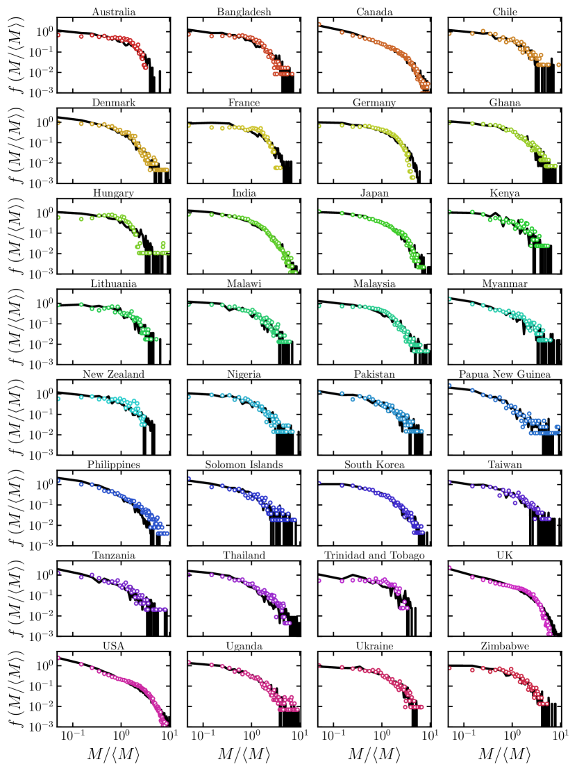
Figure S1: The empirical distribution of the scaled margin (colored open circle), along with RVM model prediction (black solid line) for $32$ countries.

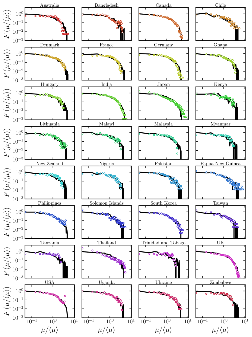
Figure S2: The empirical distribution of the scaled specific margin (colored open circle), along with RVM model prediction (black solid line) for $32$ countries.