A time-delayed model for active mode-locking

Abstract

We propose a first-principle time-delayed model for the study of active mode-locking that is devoid of restriction regarding the values of the round-trip gain and losses. It allows us to access the typical regimes encountered in semiconductor lasers and to perform an extended bifurcation analysis. Close to the harmonic resonances and to the lasing threshold, we recover the Hermite-Gauss solutions. However, the presence of the linewidth enhancement factor induces complex regimes in which even the fundamental solution becomes unstable. We discover a global bifurcation scenario in which a single pulse can jump, over a slow time scale, between the different minima of the modulation potential. Finally, we derive a Haus master equation close to the lasing threshold which shows a good agreement with the original time-delayed model.

Manipulating and shaping light is of great importance for many applications and mode-locked (ML) lasers are widely employed as high-coherence light sources [1] utilized for generating ultrashort light pulses and frequency combs [2, 3] across various applications ranging from medicine to laser metrology [4, 5, 6, 7, 8, 9]. A ML state is defined by the coherent superposition of many lasing modes in a cavity. When these modes adopt a specific phase relation, their coherent superposition may result in a train of short optical pulses whose repetition period corresponds to the time of flight in the cavity. However, such regimes are not obtained without implementing a specific mechanism favoring pulsed emission. Active mode-locking (AML) involves either an electro-optic or an acousto-optic intra-cavity modulator [10, 11, 12, 13, 14, 15], see Fig. 1 (a). If the modulation frequency is resonant with the separation between longitudinal modes, sidebands are created causing modal interactions that eventually lead to the emission of a pulse train. The main advantage of AML is its electrical tunability and the possibility to control the output pulse shape, energy and repetition rate [16, 17]. Despite their practical benefits, intensity modulators incur high costs and increased complexity. Notably, a graphene-based electro-optic modulator has been presented recently, offering improved performance and cost efficiency [17]. Furthermore, the repetition rate in AML is limited by the highest frequency at which the modulator can be driven, a few tens of GHz, and pulses cannot be as short as in passive mode-locking (PML) using a saturable absorber [18]. A way to overcome this problem is repetition-rate multiplication [19] and pulse shortening [10, 20].

Figure 1: a) A schematic of an AML ring laser containing five pulses, i.e. $\tau\approx 5T$. b) Resonance peaks (dark blue) with relative positions (turquoise) of the pulses to potential minimum. The field intensity maximum is shown as a function of the ratio of the driving period $T$ and the round-trip time $\tau$. Parameters are: $(\gamma,\,\kappa,\,\alpha,\,G_{0},\,\Gamma,\,m,\,\psi,\,\tau)=(40,\,0.4,\,0,\,1,\,1,\,0.15,\,0,\,1)$.

In this letter, we propose a time-delayed description for AML with intracavity loss or phase modulation. We note that first principle models based on time-delayed systems (TDSs) [21, 22] not only naturally allow to analyze scenarios with large gain and losses per round-trip typical of semiconductor lasers but they are also an essential tool to unveil connections between the pulsed regime and all the other possible solutions. TDS models are extensively applied to describe pulse dynamics in ring PML lasers [21], Fourier domain ML lasers [23], various PML semiconductor lasers with complex design [22, 24, 25, 26, 27, 28, 29, 30] and photonic crystal ML lasers [31], to name just a few. A sketch of the system we consider is presented in Fig. 1 (a). It consists in a ring cavity with round-trip time $\tau$ that contains a gain section (blue), a phase or an intensity modulator (red) as well as a bandpass filter (green). The latter models, beyond the intentional use of an element to control pulsewdith, the etalon effect created by parasitic reflectivities within intracavity elements. While it was shown in [32] that a small tilt of the modulator can mitigate interferometric effects and improve pulsewidth, this strategy is not always accessible, e.g. in fiber coupled systems [33].

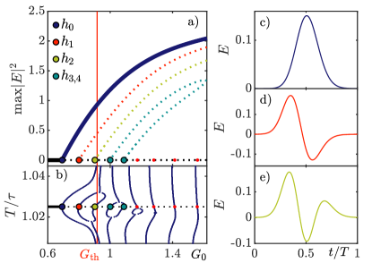
Figure 2: a) First weakly nonlinear HG modes $h_{l}$ of the TDS (1,2) emerging from the off solution. Only the $h_{0}$ mode is stable. b) Dynamics of the bifurcation points of the off solution in the $(G_{0},T/\tau)$ plane. The higher order modes emerge in pairs. Around resonance, the onset of pulses is notable below $G_{th}$. (c-e) Profiles of the modes $h_{0,1,2}$. Other parameters as in Fig. 1.

Finally, an optical isolator (black) ensures that light only propagate in one direction. The derivation of our model follows the lines of  [21] and we assume that the filter bandwidth is much smaller than the gain broadening. In this situation, the dynamical equations governing the evolution of the field $E$ at the output of the filter and that of the population inversion $G$ read

$$\frac{\dot{E}}{\gamma}+E =\sqrt{\kappa}\left[1+m\cos\left(\omega_{m}t\right)\right]e^{\left(1-i\alpha\right)G\left(t-\tau\right)/2+i\psi}E\left(t-\tau\right)\,,$$ (1)

$$\dot{G} =\Gamma\left(G_{0}-G\right)-\left(e^{G}-1\right)\left|E\right|^{2}.$$ (2)

Here, $G_{0}$ is the pumping rate, $\Gamma$ is the gain recovery rate, $\alpha$ represents the linewidth enhancement factor, $\gamma$ is the bandwidth of the spectral filter and $\psi$ is the round-trip phase. The fraction of light intensity kept in the cavity at the output coupler is $T_{o}$. For an intensity modulator, the transmission function reads $T_{i}(t)=\overline{T}+\delta T\cos\left(\omega_{m}t\right)$ with $\omega_{m}$ the modulation frequency. We approximate the effective cavity transmission for the field amplitude as given by $\sqrt{T_{o}T_{i}(t)}$, for small values of $\delta T/\overline{T}$. This leads to (1) in which the modulation depth is $m=\delta T/(2\overline{T})$ while $\kappa=T_{o}\overline{T}$. We stress that a phase modulation is simply obtained replacing $T_{i}(t)$ by $T_{p}(t)=\exp\left\{i\left[\phi_{0}+\delta\phi\cos\left(\omega_{m}t\right)\right]\right\}$.

For $m\neq 0$, the modulator creates a potential within the cavity and the ratio $n=\tau/T$ with $T=2\pi/\omega_{m}$ defines $n$ slots the potential holds for pulses, cf. Fig. 1 for $n=5$. The occurrence of resonance peaks for $n\in[1,5]$ is depicted in Fig. 1 (b) (dark blue). Following the resonance curve, the value of $\vartheta^{*}=\omega_{m}t^{*}$ (turquoise) indicates the pulse position $t^{*}$ relative to the transmission maximum. As the resonance is crossed, the pulse passes from being in advance to being delayed with respect to the latter.

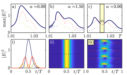
Figure 3: (a-c) Resonance curves of $h_{0}$ (blue), $h_{1}$ (red) and $h_{2}$ (green) modes, shown in i), for different values of $\alpha$. The curves reconnect and in c) a small region emerges, where both modes are unstable. leading to oscillatory states between different modes. ii) Excerpt of 400 round-trips from a numerical simulation for the $h_{0}$ mode. iii) Excerpt of 400 round-trips for an oscillatory state between $h_{0}$ and $h_{1}$, indicated by colored dotted lines. Other parameters as in Fig. 1.

First, we choose $\alpha=0$ and consider a single pulse in the cavity, i.e. $T\approx\tau$. The TDS  (1,2) correctly predicts the emergence of the family of weakly nonlinear Hermite-Gauss (HG) modes $h_{l}$ as demonstrated in  [16], that bifurcate directly from the off solution $(E,\,G)=(0,\,G_{0})$, see Fig. 2 (a). Using the path-continuation methods within ddebiftool [34], we followed the first five HG modes $h_{0}-h_{4}$ as a function of the pumping rate $G_{0}$. We notice that only the fundamental Gaussian mode $h_{0}$ is stable (solid blue line). As expected, due to the presence of the modulation, the lasing threshold for the $h_{0}$ mode is below [16] the value $G_{th}=-\log(\kappa)\simeq 0.92$ of the solitary (unmodulated) laser (cf. red vertical line). We depict in Fig. 2 (b), how the bifurcation points emerging on the off solution evolve with $G_{0}$, if the modulation period $T$ is varied. The bifurcation points (cf. colored circles in a)) occur along the horizontal black line at $T/\tau=1.025$. When $T$ is changed, the bifurcation point for the $h_{0}$ mode approaches $G_{th}$ as one leaves the resonance. There, the $h_{0}$ profile as depicted in panel c) would deform towards a simple harmonic solution. Meanwhile, the higher order modes disappear pairwise outside the resonance. Note that the resonance maxima of the different HG modes are generally not equal and also vary over $G_{0}$. The corresponding mode profiles get increasingly asymmetric far from the resonance (cf. Fig. 2 (e)). At threshold, the modes already experience an asymmetric potential if $\vartheta^{*}\neq 0$ while further asymmetry is expected due to gain dynamics for higher pumping [35, 33].

A more complex scenario is encountered for non-vanishing values of $\alpha$. We note in Fig. 2 (a,b) that the modes $h_{l}$ for $l\geq 1$ are pairwise connected. A similar recombination of modes can be observed for higher $\alpha$ values as indicated in Fig. 3. Here, the resonance curves for $h_{0}$ (blue), $h_{1}$ (red) and $h_{2}$ (green) are calculated for three different $\alpha$ values (cf. panels (a-c) and (i) for the modes profiles). For growing $\alpha$, the maximum intensity for the $h_{0}$ mode decreases and the curve starts to develop a second maximum (cf. panels (a,b)). In addition, the distance between the $h_{0}$ and $h_{1}$ curve decreases such that they reconnect via a transcritical bifurcation, see Fig. 3 (b). Further increase in $\alpha$ leads to another reconnection of the branches in the minimum, see Fig. 3 (c). Here, a regime appears where neither mode is stable. Direct numerical simulations indicate that in this region different modes interact forming complex states such as the oscillation between $h_{0}$ and $h_{1}$ modes depicted in Fig. 3 (iii).

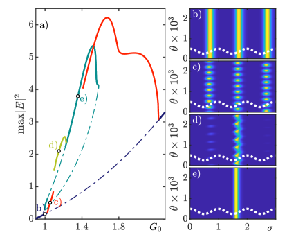
Figure 4: a) Bifurcation diagram of Eqs. (1,2) for $T=1.004$, $\Gamma=0.4$ and $\tau=3$ in the $(G_{0},\,\textrm{max}(|E|^{2}))$ plane. Solid (dash-dotted) lines denote stable (unstable) solutions, respectively. Different colors correspond to b) HML₃ solution (blue), c) modulated HML₃ solution (red), d) Modulated single-pulse solution (green), e) single-pulse solution (turquoise). Other parameters as in Fig. 1.

We turn our attention to the higher resonances and consider a regime where $\tau\approx 3T$, generating a train of three equidistant pulses, the so-called harmonic ML regime (HML₃), see Fig. 4 (b). Here, the TDS (1,2) was solved numerically and the resulting time trace is plotted using the two-time representation [36], where the fast timescale governs the dynamics within one round-trip, whereas the slow scale describes the dynamics from one round-trip to the next one. Next, we followed the obtained HML₃ solution in the parameter space using path-continuation. Figure 4 (a) presents the corresponding bifurcation diagram, where the maximum intensity is depicted as a function of $G_{0}$. There, the HML₃ solution (solid blue) becomes unstable (dotted-dashed blue) around $G_{0}=1$ in a torus bifurcation leading to a modulated HML₃ solution (solid red), see Fig. 4 (c) and Supplementary Video (SV) I. Since the path-continuation of the torus orbits is not possible, we followed the stable part of the branch using long time simulations; for some $G_{0}$, the branch loses stability and the direct numerics is unable the follow it, instead approaching the next stable attractor (yellow): a modulated single pulse solution in the three-slots potential, see Fig. 4 (d) and SV II. Note that the single pulse has a small satellite located in the left next potential slot. This solution bifurcates from a single-pulse solution (turquoise) in a supercritical torus bifurcation, cf. Fig. 4 (e). This solution forms a closed loop in the parameter space and does not seem to be connected with other stable pulse solutions. Further increasing $G_{0}$, we observe that the single pulse solution coexists with the modulated HML₃, that is connected again to the stable HML₃ solution for larger $G_{0}$. Note that several of the observed solutions were reported in  [10], considering the Haus equation with saturable gain. For lower $G_{0}$, the modulated HML₃ seems to terminate close to the single pulse branch but does not connect. The absence of any bifurcation points on the single pulse branch indicates that, if this connection exists, it is of the global nature.

To study this possible transition, we slightly change the parameters and repeat the analysis for the HML₃ solution, see Fig. 5.

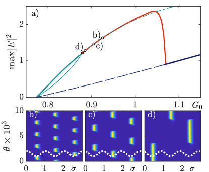
Figure 5: a) Bifurcation diagram of Eqs. (1,2) for $T=1.006$, $\tau=3$ and $\Gamma=0.5$ in the $(G_{0},\,\textrm{max}(|E|^{2}))$ plane. HML₃ (dark blue), modulated HML₃ (green) as well as single-pulse solutions (turquoise) are shown. (b-d) Three time traces in two-time representation of the modulated HML₃ close to the global bifurcation (red point). Other parameters as in Fig. 1.

Here, we focus on the range of $G_{0}$, where only modulated HML₃ (red) and single-pulse solutions (turquoise) are stable, whereas the HML₃ solution is unstable (dash-dotted blue). In Fig. 5 (b-d) three time traces are represented in two-time representation. One can observe a large increase of the modulation period as the bifurcation point (red point) is approached, indicating the global nature of this transition, cf. SV III. To identify the global bifurcation type, the scaling of the oscillation period close to the critical $G_{0}$ value is analyzed. The resulting scaling (cf. Supplement I) is an inverted square root, indicating a saddle-node infinite period bifurcation. A similar analysis for the parameter set of Fig. 4 yields the characteristic scaling of a homoclinic bifurcation, (cf. Supplement I).

Finally, to gain a better understanding of the emergence of the HG modes and to connect our analysis with former works such as  [16], we derive a Haus master equation (HME) starting from the Eqs. (1,2). The HME is a widely used theoretical model for both AML and PML that is derived from general principles using the assumptions of small gain, losses, as well as weak spectral filtering [18]. It consists in restricting the analysis of the field to a small temporal interval around the pulse whose temporal evolution, round-trip after round-trip, is described by a single partial differential equation that is then coupled to the equations responsible for the carrier dynamics. The HME was originally derived for gain media that are slowly evolving on the timescale of the cavity round-trip, resulting in a quasi-uniform gain temporal profile within the cavity. However, recent generalizations of the HME [33, 37, 38] preserve carrier memory from one round-trip towards the next, allowing for the description of complex pulse trains such as the Q-switched and harmonic ML transitions. However, when applied to a particular design, the HME often provides only qualitative predictions due to the many simplifying hypotheses involved and, in general, the question of how to derive the HME for a specific laser design still remains open. The HME appears naturally from Eqs. (1,2) using the lasing threshold $G_{th}$ as an expansion point for a multiple time scale analysis. We set $G_{0}=G_{th}(1+\epsilon^{2})$ which defines a smallness parameter $\epsilon=\sqrt{|G_{0}-G_{th}|/G_{th}}$. Further, we define multiple time scales in powers of $\epsilon$, and, after inserting all expansions in Eqs. (1,2), the resulting problems are solved order by order, see Supplement I for details. The resulting HME reads

$$\partial_{\theta}E = \left[\frac{1}{2\gamma^{2}}\partial_{\sigma}^{2}+\frac{1-i\alpha}{2}\left(G-G_{th}\right)+m\cos(\omega_{m}\sigma+\delta\theta)\right]E\,\quad$$ (3)

$$\partial_{\sigma}G = \Gamma\left(G_{0}-G\right)-\frac{1-\kappa}{\kappa}\left|E\right|^{2}\,.$$ (4)

Here, $\theta$ is a slow time scale governing the evolution between round-trips, whereas $\sigma$ is a fast time scale describing the dynamics within one round-trip with respect to the actual round-trip time $T_{c}=2\pi/\omega_{c},\,\omega_{c}=\frac{2\pi}{\tau}\frac{\gamma}{1+\gamma}$. Indeed, the actual round-trip time is slightly larger than $\tau$, leading to the round-trip drift $\delta=(\omega_{m}-\omega_{c})T_{c}$ if $\omega_{m}\neq\omega_{c}$. Note that in the good cavity limit $\kappa\rightarrow 1$, the HME (3, 4) recovers the HME derived in [39]. For $\omega_{m}=\omega_{c}$, the HME (3, 4) predicts the emergence of a family of HG modes that read $E_{l}(\sigma,\theta)=e^{-i\varpi_{l}\theta}h_{l}(\beta\sigma)$. Their branching points over the off solution occur at the gain values $G_{th}^{(l)}=G_{th}-2m+\frac{\sqrt{m}\omega_{m}}{\gamma}(2l+1)$. At resonance, the pulses are located at the minimum of the potential which is the maximum of the modulation. Ergo, the onset for AML is located below the unmodulated laser threshold $G_{th}$ by a factor proportional to the modulation depth $m$ [16]. The inverse square variance is $\beta^{2}=\omega_{m}\gamma\sqrt{m}$ and the frequency shift is $\varpi_{l}=\alpha(G_{th}^{(l)}-G_{th})/2$. We evaluated $G_{th}^{(l)}$ for the first three modes and obtained $G_{th}^{(0,1,2)}=(0.676,0.794,0.913)$. This is around $1\%$ error in comparison with the respective bifurcation points in Fig. 2 that are located at $G_{0}=(0.692,0.800,0.902)$.

In conclusion, we proposed a TDS model for AML allowing for the study of regimes of high gain and losses typical for semiconductor lasers. This approach allowed us, by using a combination of path continuation and numerical simulations, to provide a detailed bifurcation analysis of how pulses emerge and evolve in AML. We showed that our AML model does not only correctly predict the emergence of basic solutions such as the HG modes, connecting our work with previous results obtained with the HME, but also show a complex scenario of modal interaction mediated by the linewidth enhancement factor and gain dynamics. Finally, we elucidated the transitions between different dynamical regimes in the case of several pulses in a cavity, identifying two different global bifurcation scenarios.

 

Disclosures The authors declare no conflicts of interest.  

Data availability Data underlying the results presented in this paper are openly available in zenodo at http:doi.org/10.5281/zenodo.10473547, Ref. [40].  

Supplemental document See Supplement I as well as Supplementary Video I-III for supporting content.

References

- [1] L. Saito and E. Thoroh de Souza, Opt. Laser Technol. 71, 16 (2015).
- [2] D. Revin, M. Hemingway, Y. Wang, J. Cockburn, and A. Belyanin, Nat. Commun. 7, 11440 (2016).
- [3] B. Yang, H. Zhao, Z. Cao, S. Yang, Y. Zhai, J. Ou, and H. Chi, Opt. Express 28, 33220 (2020).
- [4] Y. Wang, S. Y. Set, and S. Yamashita, APL Photonics 1 (2016).
- [5] M. Horowitz, C. Menyuk, T. Carruthers, and I. Duling, J. of Lightwave Technol. 18, 1565 (2000).
- [6] R. Holzwarth, M. Zimmermann, T. Udem, and T. Hansch, IEEE J. of Quantum Electronics 37, 1493 (2001).
- [7] R. Holzwarth, T. Udem, T. W. Hänsch, J. Knight, W. Wadsworth, and P. S. J. Russell, Phys. Rev. Lett. 85, 2264 (2000).
- [8] T. Udem, R. Holzwarth, and T. W. Hänsch, Nature 416, 233 (2002).
- [9] U. Keller, Nature 424, 831 (2003).
- [10] J. Tu and J. N. Kutz, IEEE J. of Quantum Electronics 45, 282 (2009).
- [11] C. Cuadrado-Laborde, A. Diez, M. Delgado-Pinar, J. L. Cruz, and M. V. Andrés, Opt. Lett. 34, 1111 (2009).
- [12] J. Kim, J. Koo, and J. H. Lee, Photon. Res. 5, 391 (2017).
- [13] D. Kopf, F. X. Kärtner, K. J. Weingarten, and U. Keller, Opt. Lett. 19, 2146 (1994).
- [14] C. Peng, M. Yao, J. Zhang, H. Zhang, Q. Xu, and Y. Gao, Optics Communications 209, 181 (2002).
- [15] K. Zoiros, T. Houbavlis, and M. Moyssidis, Optics Communications 254, 310 (2005).
- [16] D. Kuizenga and A. Siegman, IEEE J. of Quantum Electronics 6, 694 (1970).
- [17] J. Bogusławski, Y. Wang, H. Xue, X. Yang, D. Mao, X. Gan, Z. Ren, J. Zhao, Q. Dai, G. Soboń et al., Advanced Functional Materials 28, 1801539 (2018).
- [18] H. Haus, IEEE J. Selected Topics Quantum Electron. 6, 1173 (2000).
- [19] K. Sarwar Abedin, N. Onodera, and M. Hyodo, Appl. Phys. Lett. 73, 1311 (1998).
- [20] F. X. Kärtner, D. Kopf, and U. Keller, J. Opt. Soc. Am. B 12, 486 (1995).
- [21] A. G. Vladimirov and D. Turaev, Phys. Rev. A 72, 033808 (2005).
- [22] J. Mulet and S. Balle, J. IEEE of Quantum Electronics 41, 1148 (2005).
- [23] S. Slepneva, B. Kelleher, B. O’Shaughnessy, S. Hegarty, A. Vladimirov, and G. Huyet, Opt. Express 21, 19240 (2013).
- [24] M. Marconi, J. Javaloyes, S. Balle, and M. Giudici, Phys. Rev. Lett. 112, 223901 (2014).
- [25] M. Marconi, J. Javaloyes, S. Balle, and M. Giudici, IEEE J. Sel. Top. Quantum Electron. 21, 85 (2015).
- [26] E. A. Avrutin and K. Panajotov, Materials 12, 3224 (2019).
- [27] C. Schelte, P. Camelin, M. Marconi, A. Garnache, G. Huyet, G. Beaudoin, I. Sagnes, M. Giudici, J. Javaloyes, and S. V. Gurevich, Phys. Rev. Lett. 123, 043902 (2019).
- [28] A. Bartolo, T. G. Seidel, N. Vigne, A. Garnache, G. Beaudoin, I. Sagnes, M. Giudici, J. Javaloyes, S. V. Gurevich, and M. Marconi, Opt. Lett. 46, 1109 (2021).
- [29] C. Schelte, D. Hessel, J. Javaloyes, and S. V. Gurevich, Phys. Rev. Applied 13, 054050 (2020).
- [30] J. Hausen, S. Meinecke, J. Javaloyes, S. V. Gurevich, and K. Lüdge, Phys. Rev. Applied 14, 044059 (2020).
- [31] M. Heuck, S. Blaaberg, and J. Mørk, Opt. Express 18, 18003 (2010).
- [32] D. Kuizenga and A. Siegman, IEEE J. of Quantum Electronics 6, 709 (1970).
- [33] A. M. Perego, B. Garbin, F. Gustave, S. Barland, F. Prati, and G. J. De Valcárcel, Nat. Commun 11, 311 (2020).
- [34] K. Engelborghs, T. Luzyanina, and D. Roose, ACM Trans. Math. Softw. 28, 1 (2002).
- [35] J. Javaloyes, P. Camelin, M. Marconi, and M. Giudici, Phys. Rev. Lett. 116, 133901 (2016).
- [36] G. Giacomelli and A. Politi, Phys. Rev. Lett. 76, 2686 (1996).
- [37] J. Hausen, K. Lüdge, S. V. Gurevich, and J. Javaloyes, Opt. Lett. 45, 6210 (2020).
- [38] M. Nizette and A. G. Vladimirov, Phys. Rev. E 104, 014215 (2021).
- [39] H. A. Haus, Quantum Electronics, IEEE Journal of 11, 736 (1975).
- [40] E. Koch, S. Gurevich, and J. Javaloyes, Zenodo (2024), doi: 10.5281/zenodo.10473547