BoundMPC: Cartesian Trajectory Planning with Error Bounds based on Model Predictive Control in the Joint Space

Abstract

This work presents a novel online model-predictive trajectory planner for robotic manipulators called BoundMPC. This planner allows the collision-free following of Cartesian reference paths in the end-effector's position and orientation, including via-points, within desired asymmetric bounds of the orthogonal path error. The path parameter synchronizes the position and orientation reference paths. The decomposition of the path error into the tangential direction, describing the path progress, and the orthogonal direction, which represents the deviation from the path, is well known for the position from the path-following control in the literature. This paper extends this idea to the orientation by utilizing the Lie theory of rotations. Moreover, the orthogonal error plane is further decomposed into basis directions to define asymmetric Cartesian error bounds easily. Using piecewise linear position and orientation reference paths with via-points is computationally very efficient and allows replanning the pose trajectories during the robot’s motion. This feature makes it possible to use this planner for dynamically changing environments and varying goals. The flexibility and performance of BoundMPC are experimentally demonstrated by two scenarios on a 7-DoF Kuka LBR iiwa 14 R820 robot. The first scenario shows the transfer of a larger object from a start to a goal pose through a confined space where the object must be tilted. The second scenario deals with grasping an object from a table where the grasping point changes during the robot's motion, and collisions with other obstacles in the scene must be avoided.

1 Introduction

Figure 1: Schematic of the position path planning using BoundMPC in the 3D Cartesian space. The tangential and orthogonal errors are shown for the initial position with the orthogonal error plane spanned by two basis vectors. The planned path over the planning horizon is within the asymmetric error bounds, depicted as shaded green area.

Robotic manipulators are multi-purpose machines with many different applications in industry and research, which include bin picking [1], physical human-robot interaction [2], and industrial processes like welding [3]. During the execution of these applications, various constraints have to be considered, such as safety bounds, collision avoidance, and kinematic and dynamic limitations. In general, this leads to challenging trajectory-planning problems. A well-suited control framework for such applications is model predictive control (MPC) [4]. Using MPC, the control action is computed by optimizing an objective function over a finite planning horizon at every time step while respecting all constraints. Online trajectory planning with MPC is particularly useful for robots acting in dynamically changing environments. Especially when there is uncertainty about actors in the scene, it is crucial to appropriately react to changing situations, e.g., when interacting with humans [5].

Robotic tasks are often specified as Cartesian reference paths, which raises the need for path-following controllers [6]. Dynamic replanning of such reference paths requires an online trajectory planner to react to dynamically changing environments. A reference path is not parametrized in time but by a path parameter, thus, separating the control problem in a spatial and a temporal approach. It is advantageous to decompose the error between the current position and the desired reference path point [7] into a tangential error, representing the error along the path and an orthogonal error. The tangential error is minimized to progress along the path quickly while the orthogonal error is bounded [8]. Several applications benefit from the concept of via-points. In this context, a via-point is a point along the path where zero path error is desired to pass this point exactly.

An illustrative example is an autonomous car racing along a known track. The center line of the track is the reference path. The path progress, in combination with the minimization of the tangential error, ensures fast progress along the path. The orthogonal error is the deviation from the center line, which is bounded by the width of the track. The orthogonal error can be leveraged to optimize the forward velocity speed along the path, e.g., in corners where it is advantageous to deviate from the center line of the track. A via-point may be specified when passing other cars along the track. The allowed orthogonal error becomes zero to avoid collisions and allow safe racing along the track.

Providing the reference path in Cartesian space is intuitive but, due to the complex robot kinematics, complicates the trajectory planning compared to planning in the robot's joint space. Cartesian reference paths have the additional advantage of simplifying collision avoidance. However, orientation representations are difficult to use in optimization-based planners. Therefore, existing solutions use simplifications that limit performance [9].

This work introduces a novel online trajectory planner in the joint space, BoundMPC, to follow a Cartesian reference path with the robot's end effector while bounding the orthogonal path error. Furthermore, position and orientation reference paths with via-points are considered. A schematic drawing of the geometric relationships is shown in fig. 1. By bounding the orthogonal path error and minimizing the tangential path error, the MPC can find the optimal trajectory according to the robot dynamics and other constraints. Simple piecewise linear reference paths with via-points are used to simplify online replanning, and (asymmetric) polynomial error bounds allow us to adapt to different scenarios and obstacles quickly. The end-effector's position and orientation reference paths are parameterized by the same path parameter, ensuring synchronicity at the via-points. The Lie theory for rotations is employed to describe the end effector's orientation, which yields a novel way to decompose and constrain the orientation path error. Moreover, the decomposition of the orthogonal error using the desired basis vectors of the orthogonal error plane allows for meaningful asymmetric bounding of both position and orientation path errors.

The paper is organized as follows: Related work is summarized in section 2, and the contributions extending the state of the art are given in section 3. The general MPC framework BoundMPC is developed in section 4. The use of a piecewise linear reference path and its implications are presented in section 6. Afterward, section 7 shows the online replanning. The implementation details for the simulations and experiments are given in section 8. Section 9 deals with the parameter tuning of the MPC. Two experimental scenarios on a 7-DoF Kuka LBR iiwa 14 R820 robot are demonstrated in section 10, which emphasize the ability of BoundMPC to replan trajectories online during the robot's motion and to specifically bound the orthogonal errors asymmetrically. Section 11 gives some conclusions and an outlook on future research activities.

2 Related Work

Path and trajectory planning in robotics is an essential topic with many different solutions, such as sampling-based planners [10, 11, 12], learning-based planners [13, 14, 15], and optimization-based planners [7, 6, 4], which can be further classified into offline and online planning. Online planning is needed to be able to react to dynamically changing environments. Sampling-based planners have the advantage of being probabilistically complete, meaning they will eventually find a solution if the problem is feasible. However, online planning is limited by computational costs and the need to smooth the obtained trajectories [16, 17]. Constrained motion planning with sampling-based methods is discussed in [18]. Optimization-based trajectory planners, such as TrajOpt [19], CHOMP [20] and CIAO [21], take dynamics and collision avoidance into account. However, they are generally too slow for online planning due to the nonconvexity of the planning problems. Receding horizon control plans a path for a finite horizon starting at the current state to reduce computational complexity. For example, CIAO-MPC [21] extends CIAO to receding horizon control for point-to-point motions.

More complex applications require the robot to follow a reference path. Receding horizon control in this setting was demonstrated for quadrotor racing in [8, 7] and robotic manipulators in [9]. Additionally, [7] includes via-points in their framework to safely pass the gates along the racing path. Adapting the current reference path during the motion to react to a changing environment and a varying goal is crucial. While, in theory, the developed MPC frameworks in [9, 7, 8, 22] could handle a change in the reference path, this still needs to be demonstrated for industrial manipulators. Alternatively, the orthogonal error bounds can be adapted to reflect a dynamic change in the environment, as done in [8].

To be able to use the path following formulations, an arc-length parametrized path is needed. Since the system dynamics are parametrized in time, a reformulation is needed to couple the reference path to the system dynamics as done in [23, 8, 24, 25, 6]. Such a coupling allows for a very compact formulation but complicates constraint formulations. Therefore, [22] decouples the system dynamics from the path and uses the objective function to minimize the tangential path error to ensure that the path system is synchronized to the system dynamics.

Tracking the reference path by the planner results in a path error. The goal of the classical path following control is to minimize this error [4, 9], which is desirable if the reference path is optimal. Since optimal reference paths are generally not trivial, exploiting the path error to improve the performance has been considered in [8, 7]. Further control on utilizing the path error is given by decomposing it into tangential and orthogonal components. To safely traverse via-points, [7] uses a dynamical weighting of the orthogonal path error, achieving collision-free trajectories. Furthermore, the orthogonal path error lies in the plane orthogonal to the path and can thus be decomposed further using basis vectors of the plane. This way, surface-based path following was proposed in [26], where the direction orthogonal to the surface was used to assign a variable stiffness. The choice of basis vectors is application specific. Concretely, [8] uses the Frenet-Serret frame to decompose the orthogonal path error. It provides a continuously changing frame along the path but is not defined for path sections with zero curvature. An alternative to the Frenet-Serret frame is the parallel transport frame used in [27]. The decomposition of the orthogonal error allows for asymmetric bounding in different directions of the orthogonal error plane, but this has yet to be demonstrated in the literature.

Many path-following controllers only consider a position reference trajectory and, thus, a position path error. For quadrotors, this is sufficient since the orientation is given by the dynamics [7]. The orientation was included in ([28] astudilloPositionOrientationTunnelFollowing2022,  astudilloVaryingRadiusTunnelFollowingNMPC2022) for robotic manipulators but was assumed to be small. The orientation in [6] is even considered constant. In [26], the orientation is set relative to the surface and is not freely optimized. Thus, orientation reference paths without limits on the size of the path error have yet to be treated in the literature. Furthermore, a decomposition of the orientation path error analogous to the position path error is missing in the literature, which can further improve the performance of path-following controllers. In this work, orientation reference paths are included using the Lie theory for rotations, which is beneficial since the rotation propagation can be linearized. In [29], this property was exploited for pose estimation based on the theory in [30]. Forster et al. (forsterOnManifoldPreintegrationRealTime2017) use the same idea for visual-inertial odometry. In this work, the Lie theory for rotations is exploited to decompose the orientation path error and the propagation of this error over time.

3 Contributions

The proposed MPC framework BoundMPC combines concepts discussed in section 2 in a novel way. It uses a receding horizon implementation to follow a reference path in the position and orientation with asymmetric error bounds in distinct orthogonal error directions. A path parameter system similar to [22] ensures path progress. Using linear reference paths with via-points yields a simple representation of reference paths and allows for fast online replanning. Additionally, the orientation has a distinct reference path, and an assumption on small orientation path errors, as in previous work, is not required. The novel asymmetric error bounds allow more control over trajectory generation and obstacle avoidance. Through its simplicity of only providing the desired via-points, BoundMPC finds the optimal position and orientation path within the given error bounds. The main contributions are:

• A path-following MPC framework to follow position and orientation paths with synchronized via-points is developed. The robot kinematics are considered in the optimization problem such that the joint inputs are optimized while adhering to (asymmetric) Cartesian constraints.

• The orientation is represented using the Lie theory for rotations to allow an efficient decomposition and bounding of the orientation errors.

• Piecewise linear position and orientation reference paths with via-points can be replanned online to quickly react to dynamically changing environments and new goals during the robot's motion.

• The framework is demonstrated on a 7-DoF Kuka LBR iiwa 14 R820 manipulator with planning times less than $100\text{\,}\mathrm{ms}$. A video of the experiments can be found at https://www.acin.tuwien.ac.at/42d0/.

4 BoundMPC Formulation

This section describes the BoundMPC formulation, which is a path-following concept for Cartesian position and orientation reference paths. This concept is schematically illustrated in fig. 1. The proposed formulation computes a trajectory in the joint space, requiring an underlying torque controller to follow the planned trajectory.

First, the formulation of the dynamical systems, i.e., the robotic manipulator and the jerk input system, is introduced. Second, the orientation representation based on Lie algebra and its linearization is used to calculate the tangential and orthogonal orientation path errors based on arc-length parameterized reference paths. A similar decomposition is also introduced for the position path error, finally leading to the optimal control problem formulation.

4.1 Dynamical System

The robotic manipulator dynamics for $n$ joints are described in the joint positions $\mathbf{q}\in\mathbb{R}^{n}$, velocities $\dot{\mathbf{q}}\in\mathbb{R}^{n}$, and accelerations $\ddot{\mathbf{q}}\in\mathbb{R}^{n}$ as the rigid-body model

$$\mathbf{M}(\mathbf{q})\ddot{\mathbf{q}}+\mathbf{C}(\mathbf{q},\dot{\mathbf{q}})\dot{\mathbf{q}}+\mathbf{g}(\mathbf{q})=\bm{\tau}\text{~{},}$$ (1)

with the mass matrix $\mathbf{M}(\mathbf{q)}$, the Coriolis matrix $\mathbf{C}(\mathbf{q},\dot{\mathbf{q}})$, the gravitational forces $\mathbf{g}(\mathbf{q})$, and the joint input torque $\bm{\tau}\in\mathbb{R}^{n}$. For trajectory following control, the computed-torque controller [32]

$$\bm{\tau}= \mathbf{M}(\mathbf{q})\left(\ddot{\mathbf{q}}_{\mathrm{d}}(t)-\mathbf{K}_{2}\dot{\mathbf{e}}_{\mathrm{q}}-\mathbf{K}_{1}\mathbf{e}_{\mathrm{q}}-\mathbf{K}_{0}\int\mathbf{e}_{\mathrm{q}}\mathrm{d}t\right)$$ (2)

$$+\mathbf{C}(\mathbf{q},\dot{\mathbf{q}})\dot{\mathbf{q}}+\mathbf{g}(\mathbf{q})\text{~{},}$$

with the desired joint-space trajectory $\mathbf{q}_{\mathrm{d}}(t)$ and its time derivatives, is applied to eq. 1. The tracking error $\mathbf{e}_{\mathrm{q}}=\mathbf{q}-\mathbf{q}_{\mathrm{d}}$ is exponentially stabilized in the closed-loop system eq. 1, eq. 2 by choosing suitable matrices $\mathbf{K}_{0}$, $\mathbf{K}_{1}$, and $\mathbf{K}_{2}$, typically by pole placement.

4.1.1 Joint Jerk Parametrization

To obtain the desired trajectory $\mathbf{q}_{\mathrm{d}}(t)$, a joint jerk input signal ${\mathop{\kern 0.0pt\mathbf{q}}\limits^{\makebox[0.0pt][c]{\vbox to-1.4pt{\kern-2.0pt\hbox{...}\vss}}}}_{\mathrm{d}}(t)$ is introduced, which is parameterized using hat functions similar to [33]. The hat functions $H_{k}(t)$, $k=0,\ldots,K-1$, given by

$$H_{k}(t)=\begin{cases}\frac{t-t_{k}}{T_{\mathrm{s}}}&t_{k}\leq t<t_{k}+T_{\mathrm{s}}\\ \frac{t_{k}+2T_{\mathrm{s}}-t}{T_{\mathrm{s}}}&t_{k}+T_{\mathrm{s}}\leq t\leq t_{k}+2T_{\mathrm{s}}\\ 0&\text{otherwise}\text{~{},}\\ \end{cases}$$ (3)

are parametrized by the starting time $t_{k}$ and the width $2T_{\mathrm{s}}$. The index $k$ refers to an equidistant time grid $t_{k}=kT_{\mathrm{s}}$ on the continuous time $t$. For each joint at the discretization points, the desired jerk values are denoted by the vectors $\mathbf{j}_{k}\in\mathbb{R}^{n}$, $k=0,\ldots,K-1$. Thus, the continuous joint jerk input

$${\mathop{\kern 0.0pt\mathbf{q}}\limits^{\makebox[0.0pt][c]{\vbox to-1.4pt{\kern-2.0pt\hbox{...}\vss}}}}_{\mathrm{d}}(t)=\sum_{k=0}^{K-1}H_{k}(t+T_{s})\mathbf{j}_{k}$$ (4)

results from the summation of all hat functions over the considered time interval. The joint jerk eq. 4 is a linear interpolation of the joint jerk values $\mathbf{j}_{k}$. The desired trajectory for the joint accelerations $\ddot{\mathbf{q}}_{\mathrm{d}}(t)$, joint velocities $\dot{\mathbf{q}}_{\mathrm{d}}(t)$, and joint positions $\mathbf{q}_{\mathrm{d}}(t)$ are found analytically by integrating eq. 4 with respect to the time $t$ for $t_{0}=0$

$$\ddot{\mathbf{q}}_{\mathrm{d}}(t)=\; \ddot{\mathbf{q}}_{\mathrm{d},0}+\sum_{k=0}^{K-1}\int_{0}^{t}H_{k}(\tau+T_{\mathrm{s}})\mathrm{d}\tau\mathbf{j}_{k}$$ (5a)

$$\dot{\mathbf{q}}_{\mathrm{d}}(t)=\; \dot{\mathbf{q}}_{\mathrm{d},0}+\ddot{\mathbf{q}}_{\mathrm{d},0}t+\sum_{k=0}^{K-1}\iint_{0}^{t}H_{k}(\tau+T_{\mathrm{s}})\mathrm{d}\tau\mathbf{j}_{k}$$ (5b)

$$\begin{split}\mathbf{q}_{\mathrm{d}}(t)=\;&\mathbf{q}_{\mathrm{d},0}+\dot{\mathbf{q}}_{\mathrm{d},0}t+\ddot{\mathbf{q}}_{\mathrm{d},0}\frac{t^{2}}{2}\\ &+\sum_{k=0}^{K-1}\iiint_{0}^{t}H_{k}(\tau+T_{\mathrm{s}})\mathrm{d}\tau\mathbf{j}_{k}\text{~{}.}\end{split}$$ (5c)

The integration constants $\mathbf{q}_{\mathrm{d}}(0)=\mathbf{q}_{\mathrm{d},0}$, $\dot{\mathbf{q}}_{\mathrm{d}}(0)=\dot{\mathbf{q}}_{\mathrm{d},0}$, and $\ddot{\mathbf{q}}_{\mathrm{d}}(0)=\ddot{\mathbf{q}}_{\mathrm{d},0}$ are given by the initial values at the time $t_{0}=0$.

4.1.2 Linear Time-Invariant System

In the following, eq. 5 is described by a linear time-invariant (LTI) system with the state $\mathbf{x}^{\mathrm{T}}=[\mathbf{q}_{\mathrm{d}}^{\mathrm{T}},\dot{\mathbf{q}}_{\mathrm{d}}^{\mathrm{T}},\ddot{\mathbf{q}}_{\mathrm{d}}^{\mathrm{T}}]$. The corresponding discrete-time LTI system with the sampling time $T_{\mathrm{s}}$ then reads as

$$\mathbf{x}_{k+1}=\mathbf{\Phi}\mathbf{x}_{k}+\mathbf{\Gamma}_{0}\mathbf{u}_{k}+\mathbf{\Gamma}_{1}\mathbf{u}_{k+1}\text{~{},}$$ (6)

with the state $\mathbf{x}_{k}$ and the input $\mathbf{u}_{k}=\mathbf{j}_{k}$.

4.1.3 Robot Kinematics

The forward kinematics of the robot are mappings from the joint space to the Cartesian space and describe the Cartesian pose of the robot's end effector. Given the joint positions $\mathbf{q}$ of the robot, the Cartesian position map for the forward kinematics reads as $\mathbf{p}_{\mathrm{c}}(\mathbf{q}):\mathbb{R}^{n}\rightarrow\mathbb{R}^{3}$ and for the orientation $\mathbf{R}_{\mathrm{c}}(\mathbf{q}):\mathbb{R}^{n}\rightarrow\mathbb{R}^{3\times 3}$, with the rotation matrix $\mathbf{R}_{\mathrm{c}}$.

By using the geometric Jacobian $\mathbf{J}(\mathbf{q})\in\mathbb{R}^{6\times n}$, the Cartesian velocity $\mathbf{v}$ and the angular velocity $\bm{\omega}$ of the end effector are related to the joint velocity $\dot{\mathbf{q}}$ by

$$\begin{bmatrix}\mathbf{v}\\ \bm{\omega}\\ \end{bmatrix}=\mathbf{J}(\mathbf{q})\dot{\mathbf{q}}\text{~{}.}$$ (7)

If $n>6$, the robot is kinematically redundant and the Jacobian $\mathbf{J}(\mathbf{q})$ becomes a non-square matrix. Redundant robots, such as the Kuka LBR iiwa 14 R820 used in this work, have a joint nullspace, which has to be considered for planning and control. To this end, the nullspace projection matrix [34]

$$\mathbf{P}_{\mathrm{n}}(\mathbf{q})=\mathbf{I}-\mathbf{J}^{\dagger}(\mathbf{q})\mathbf{J}(\mathbf{q})\text{~{},}$$ (8)

is used to project the joint configuration into the nullspace, where $\mathbf{I}$ denotes the identity matrix and $\mathbf{J}^{\dagger}(\mathbf{q})=\mathbf{J}^{\mathrm{T}}(\mathbf{q})\left(\mathbf{J}(\mathbf{q})\mathbf{J}^{\mathrm{T}}(\mathbf{q})\right)^{-1}$ is the right pseudo-inverse of the end-effector Jacobian. This yields

$$\dot{\mathbf{q}}_{\mathrm{n}}=\mathbf{P}_{\mathrm{n}}(\mathbf{q})\dot{\mathbf{q}}$$ (9)

as the nullspace joint velocity.

4.2 Orientation Representation

The orientation of the end effector in the Cartesian space can be represented in different ways, such as rotation matrices, quaternions, and Euler angles. In this work, the Lie algebra

$$\bm{\tau}=\theta\mathbf{u}$$ (10)

of the rotation matrix $\mathbf{R}$ is used. An orientation is thus specified by an angle $\theta$ around the unit length axis $\mathbf{u}$. The most relevant results of the Lie theory for rotations, utilized in this work, are summarized from [30] in the following.

4.2.1 Mappings

To transform a rotation matrix $\mathbf{R}$ into its equivalent (non-unique) element $\bm{\tau}$ in the Lie space, the exponential and logarithmic mappings

$$\text{Exp}:\quad \mathbb{R}^{3}\rightarrow\mathbb{R}^{3\times 3}:\bm{\tau}\rightarrow\mathbf{R}=\text{Exp}(\bm{\tau})$$ (11)

$$\text{Log}:\quad \mathbb{R}^{3\times 3}\rightarrow\mathbb{R}^{3}:\mathbf{R}\rightarrow\bm{\tau}=\text{Log}(\mathbf{R})$$ (12)

are used, with the definitions

$$\text{Exp}(\theta\mathbf{u}) =\mathbf{I}+\sin(\theta)[\mathbf{u}]_{\times}+(1-\cos(\theta))[\mathbf{u}]^{2}_{\times}$$ (13)

$$[\text{Log}(\mathbf{R})]_{\times} =\frac{\phi(\mathbf{R}-\mathbf{R}^{\mathrm{T}})}{2\sin(\phi)}\text{~{},}$$ (14)

the identity matrix $\mathbf{I}$, and $\phi=\cos^{-1}(\frac{\text{trace}(\mathbf{R})-1}{2})$. The operator

$$\left[\mathbf{u}\right]_{\times}=\left[\begin{bmatrix}u_{x}\\ u_{y}\\ u_{z}\end{bmatrix}\right]_{\times}=\begin{bmatrix}0&-u_{z}&u_{y}\\ u_{z}&0&-u_{x}\\ -u_{y}&u_{x}&0\\ \end{bmatrix}$$ (15)

converts a vector into a skew-symmetric matrix.

4.2.2 Concatenation of Rotations

A rotation matrix may results from the concatenation of multiple rotation matrices. An example are the Euler angles which are the result of three consecutive rotations around distinct rotation axes. Concretely, let us assume that

$$\mathbf{R}=\mathbf{R}_{3}\mathbf{R}_{2}\mathbf{R}_{1}=\text{Exp}(\bm{\tau}_{3})\text{Exp}(\bm{\tau}_{2})\text{Exp}(\bm{\tau}_{1})=\text{Exp}(\bm{\tau})$$ (16)

is the combination of the rotation matrices $\mathbf{R}_{1}$, $\mathbf{R}_{2}$, and $\mathbf{R}_{3}$. By using the Lie theory for rotations, eq. 16 can be approximated around $\mathbf{R}_{2}$ as [30]

$$\bm{\tau} =\text{Log}(\mathbf{R}_{3}\mathbf{R}_{2}\mathbf{R}_{1})$$ (17)

$$\approx\text{Log}(\mathbf{R}_{3}\mathbf{R}_{2})+\mathbf{J}_{\mathrm{r}}^{-1}(\text{Log}(\mathbf{R}_{3}\mathbf{R}_{2}))\bm{\tau}_{1}$$

$$\approx\bm{\tau}_{2}+\mathbf{J}_{\mathrm{l}}^{-1}(\bm{\tau}_{2})\bm{\tau}_{3}+\mathbf{J}_{\mathrm{r}}^{-1}(\text{Log}(\mathbf{R}_{3}\mathbf{R}_{2}))\bm{\tau}_{1}\text{~{},}$$

where the left and right inverse Jacobians

$$\mathbf{J}_{\mathrm{l}}^{-1}(\bm{\tau}) =\mathbf{I}-\frac{1}{2}[\bm{\tau}]_{\times}+\left(\frac{1}{\theta^{2}}-\frac{1+\cos\theta}{2\theta\sin\theta}\right)[\bm{\tau}]_{\times}^{2}$$ (18)

$$\mathbf{J}_{\mathrm{r}}^{-1}(\bm{\tau}) =\mathbf{I}+\frac{1}{2}[\bm{\tau}]_{\times}+\left(\frac{1}{\theta^{2}}-\frac{1+\cos\theta}{2\theta\sin\theta}\right)[\bm{\tau}]_{\times}^{2}$$ (19)

are defined using $\theta=\lVert\bm{\tau}\rVert_{2}$. Approximations around $\mathbf{R}_{1}$ and $\mathbf{R}_{3}$ are obtained analogously to eq. 17. Note that for transposed rotation matrices the additions in eq. 17 become subtractions.

4.3 Reference Path Formulation

In this work, each path point is given as a Cartesian pose, which motivates a separation of the position and orientation path as $\bm{\pi}_{\mathrm{p}}(\phi)\in\mathbb{R}^{3}$ and $\bm{\pi}_{\mathrm{o}}(\phi)\in\mathbb{R}^{3}$, respectively, with the same path parameter $\phi$. The position reference path $\bm{\pi}_{\mathrm{p}}(\phi)$ is assumed to be arc-length parametrized. The arc-length parametrization implies $\lVert\frac{\partial}{\partial\phi}\bm{\pi}_{\mathrm{p}}\rVert_{2}=\lVert\bm{\pi}^{\prime}_{\mathrm{p}}\rVert_{2}=1,\forall\phi\in[0,\phi_{\mathrm{f}}]$, where $\phi_{\mathrm{f}}$ is the total arc length of the path. The orientation path uses the same path parameter $\phi$ and is therefore, in general, not arc-length parametrized. To couple the two paths, the orientation path $\bm{\pi}_{\mathrm{o}}(\phi)$ is parametrized such that the via-points coincide with the position path $\bm{\pi}_{\mathrm{p}}(\phi)$ and the orientation path also ends at $\phi_{\mathrm{f}}$. Hence, the orientation path derivative is in general not normalized, which will become important later.

4.4 Path Error

In this section, the position and orientation path errors are computed and decomposed based on the tangential path directions $\bm{\pi}_{\mathrm{p}}^{\prime}=\frac{\partial}{\partial\phi}\bm{\pi}_{\mathrm{p}}$ and $\bm{\pi}_{\mathrm{o}}^{\prime}=\frac{\partial}{\partial\phi}\bm{\pi}_{\mathrm{o}}$. First, the position path error and its decomposition are described. Second, the orientation path error is decomposed similarly using the formulation from section 4.2.

4.4.1 Position Path Error

The position path error between the current end-effector position $\mathbf{p}_{\mathrm{c}}(\mathbf{q})$ and the reference path in the Cartesian space

$$\mathbf{e}_{\mathrm{p}}(\mathbf{q},\phi(t))=\mathbf{p}_{\mathrm{c}}(\mathbf{q})-\bm{\pi}_{\mathrm{p}}(\phi(t))$$ (20)

is a function of the joint positions $\mathbf{q}$ and the path parameter $\phi(t)$ using the forward kinematics $\mathbf{p}_{\mathrm{c}}(\mathbf{q})$ of the robot.

Figure 2: Position path error decomposition into the orthogonal and tangential path direction. The black rectangle visualizes the orthogonal error plane spanned by the basis vectors $\mathbf{b}_{\mathrm{p,1}}$ and $\mathbf{b}_{\mathrm{p,2}}$. The current reference path position is $\bm{\pi}_{\mathrm{p}}(\phi(t))$. The blue lines indicate the errors of the current end-effector position $\mathbf{p}_{\mathrm{c}}(t)$. The error bounds are indicated by the green rectangle, which is offset from the path by $\mathbf{e}_{\mathrm{p,\mathrm{off}}}$.

4.4.2 Position Path Error Decomposition

The position path error eq. 20 is decomposed into a tangential and an orthogonal error. Figure 2 shows a visualization of the geometric relations. The tangential part

$$\mathbf{e}_{\mathrm{p}}^{||}(\mathbf{q},\phi(t))=\left(\bm{\pi}^{\prime}_{\mathrm{p}}(\phi(t))^{\mathrm{T}}\mathbf{e}_{\mathrm{p}}(\mathbf{q},\phi(t)))\right)\bm{\pi}^{\prime}_{\mathrm{p}}(\phi(t))$$ (21)

is the projection onto the tangent $\bm{\pi}^{\prime}_{\mathrm{p}}(\phi(t))$ of the reference path. Thus, the remaining error is the orthogonal path error, reading as

$$\mathbf{e}_{\mathrm{p}}^{\bot}(\mathbf{q},\phi(t))=\mathbf{e}_{\mathrm{p}}(\mathbf{q},\phi(t))-\mathbf{e}_{\mathrm{p}}^{||}(\mathbf{q},\phi(t))\text{~{}.}$$ (22)

The time derivatives of eq. 21 and eq. 22 yield

$$\dot{\mathbf{e}}_{\mathrm{p}}=\; \frac{\mathrm{d}}{\mathrm{d}t}\mathbf{p}_{\mathrm{c}}(\mathbf{q})-\bm{\pi}_{\mathrm{p}}^{\prime}(\phi(t))\dot{\phi}(t)$$ (23a)

$$\begin{split}\dot{\mathbf{e}}_{\mathrm{p}}^{||}=\;&\bigl{(}\bigl{(}\bm{\pi}_{\mathrm{p}}^{\prime\prime}(\phi(t))\dot{\phi}(t)\bigl{)}^{\mathrm{T}}\mathbf{e}_{\mathrm{p}}(\mathbf{q},\phi(t))\bigl{)}\bm{\pi}_{\mathrm{p}}^{\prime}(\phi(t))\\ &+\left(\bm{\pi}_{\mathrm{p}}^{\prime}(\phi(t))^{\mathrm{T}}\dot{\mathbf{e}}_{\mathrm{p}}(\mathbf{q},\phi(t))\right)\bm{\pi}_{\mathrm{p}}^{\prime}(\phi(t))\\ &+\left(\bm{\pi}_{\mathrm{p}}^{\prime}(\phi(t))^{\mathrm{T}}\mathbf{e}_{\mathrm{p}}(\mathbf{q},\phi(t))\right)\bm{\pi}_{\mathrm{p}}^{\prime\prime}(\phi(t))\dot{\phi}(t)\end{split}$$ (23b)

$$\dot{\mathbf{e}}_{\mathrm{p}}^{\bot}=\; \dot{\mathbf{e}}_{\mathrm{p}}(\mathbf{q},\phi(t))-\dot{\mathbf{e}}_{\mathrm{p}}^{||}(\mathbf{q},\phi(t))\text{~{}.}$$ (23c)

In the following, the function arguments will be omitted for clarity of presentation. The orthogonal path error $\mathbf{e}_{\mathrm{p}}^{\bot}$ from eq. 22 is further decomposed using the orthonormal basis vectors $\mathbf{b}_{\mathrm{p,1}}$ and $\mathbf{b}_{\mathrm{p,2}}$ of the orthogonal error plane. The orthogonal position path errors $\mathbf{e}_{\mathrm{p}}^{\bot,1}$, $\mathbf{e}_{\mathrm{p}}^{\bot,2}$ are then obtained by projection onto these basis vectors as

$$\mathbf{e}_{\mathrm{p,\mathrm{proj}}}^{\bot} =\begin{bmatrix}e_{\mathrm{p,\mathrm{proj},1}}^{\bot}\\ e_{\mathrm{p,\mathrm{proj},2}}^{\bot}\end{bmatrix}=\begin{bmatrix}\mathbf{b}_{\mathrm{p,1}}^{\mathrm{T}}\\ \mathbf{b}_{\mathrm{p,2}}^{\mathrm{T}}\end{bmatrix}\mathbf{e}^{\bot}_{\mathrm{p}}$$ (24a)

$$\mathbf{e}_{\mathrm{p}}^{\bot,i} =e_{\mathrm{p,proj},i}^{\bot}\mathbf{b}_{\mathrm{p},i}\text{~{},~{}}i=1,2\text{~{}.}$$ (24b)

The basis vectors $\mathbf{b}_{\mathrm{p,1}}$ and $\mathbf{b}_{\mathrm{p,2}}$ are obtained using the Gram-Schmidt procedure by providing a desired basis vector $\mathbf{b}_{\mathrm{p,d}}$ and using the reference velocity vector $\mathbf{v}_{\mathrm{r}}=\bm{\pi}^{\prime}_{\mathrm{p}}(\phi(t))$, leading to

$$\mathbf{w}(\mathbf{v}_{\mathrm{r}},\mathbf{b}_{\mathrm{p,d}}) =\left(\frac{\mathbf{v}_{\mathrm{r}}^{\mathrm{T}}}{\lVert\mathbf{v}_{\mathrm{r}}\rVert_{2}}\mathbf{b}_{\mathrm{p,d}}\right)\frac{\mathbf{v}_{\mathrm{r}}}{\lVert\mathbf{v}_{\mathrm{r}}\rVert_{2}}$$ (25a)

$$\mathbf{u}(\mathbf{v}_{\mathrm{r}},\mathbf{b}_{\mathrm{p,d}}) =\mathbf{b}_{\mathrm{p,d}}-\mathbf{w}(\mathbf{v}_{\mathrm{r}},\mathbf{b}_{\mathrm{p,d}})$$ (25b)

$$\mathbf{b}_{\mathrm{p,1}} =\frac{\mathbf{u}(\mathbf{v}_{\mathrm{r}},\mathbf{b}_{\mathrm{p,d}})}{\lVert\mathbf{u}(\mathbf{v}_{\mathrm{r}},\mathbf{b}_{\mathrm{p,d}})\rVert_{2}}$$ (25c)

as the first normalized basis vector. The cross product $\mathbf{b}_{\mathrm{p,2}}=\mathbf{v}_{\mathrm{r}}\times\mathbf{b}_{\mathrm{p,1}}$ gives the second basis vector. Note that $\mathbf{b}_{\mathrm{p,d}}$ and $\mathbf{v}_{\mathrm{r}}$ must be linearly independent.

4.4.3 Orientation Path Error

In the following, the orientation path errors are derived using rotation matrices. Then the errors are approximated by applying the Lie theory for rotations from section 4.2. The orientation path error between the planned and the reference path

$$\mathbf{e}_{\mathrm{o}}(t)=\text{Log}\left(\mathbf{R}_{\mathrm{c}}(t)\mathbf{R}^{\mathrm{T}}_{\mathrm{r}}(\phi(t))\right)$$ (26)

is a function of the time $t$, with the rotation matrix representation of the orientation reference path $\mathbf{R}_{\mathrm{r}}(\phi(t))=\text{Exp}(\bm{\pi}_{\mathrm{o}}(\phi(t)))$ and the current state rotation matrix $\mathbf{R}_{\mathrm{c}}(t)=\mathbf{R}_{\mathrm{c}}(\mathbf{q}(t))$. These rotation matrices are related to the respective angular velocities $\bm{\omega}_{\mathrm{c}}$ and $\bm{\omega}_{\mathrm{r}}$ in the form

$$\dot{\mathbf{R}}_{\mathrm{c}}(t) =[\bm{\omega}_{\mathrm{c}}(t)]_{\times}\mathbf{R}_{\mathrm{c}}(t)$$ (27a)

$$\frac{\partial\mathbf{R}_{\mathrm{r}}(\phi)}{\partial\phi} =[\bm{\omega}_{\mathrm{r}}(\phi(t))]_{\times}\mathbf{R}_{\mathrm{r}}(\phi(t))\text{~{},}$$ (27b)

where the reference path depends on the path parameter $\phi(t)$. For constant angular velocities $\bm{\omega}_{\mathrm{c}}$ and $\bm{\omega}_{\mathrm{r}}$, the closed-form solutions for eq. 27 over a time span $\Delta t$ exist in the form

$$\mathbf{R}_{\mathrm{c}}(t+\Delta t) =\text{Exp}(\bm{\omega}_{\mathrm{c}}\Delta t)\mathbf{R}_{\mathrm{c}}(t)$$ (28a)

$$\mathbf{R}_{\mathrm{r}}(\phi(t)+\Delta\phi) =\text{Exp}(\bm{\omega}_{\mathrm{r}}\Delta\phi)\mathbf{R}_{\mathrm{r}}(\phi(t))\text{~{},}$$ (28b)

with $\Delta\phi=\phi(t+\Delta t)-\phi(t)$. Using eq. 17 and $\Delta\phi\approx\dot{\phi}(t)\Delta t$, the orientation path error $\mathbf{e}_{\mathrm{o}}(t)$ propagates as

$$\mathbf{e}_{\mathrm{o}} (t+\Delta t)$$ (29)

$$=\text{Log}(\text{Exp}(\bm{\omega}_{\mathrm{c}}\Delta t)\mathbf{R}_{\mathrm{c}}(t)\mathbf{R}^{\mathrm{T}}_{\mathrm{r}}(\phi(t))\text{Exp}(\bm{\omega}_{\mathrm{r}}\Delta\phi)^{\mathrm{T}})$$

$$\approx\mathbf{e}_{\mathrm{o}}(t)+\Delta t\big{[}\mathbf{J}_{\mathrm{l}}^{-1}(\mathbf{e}_{\mathrm{o}}(t))\bm{\omega}_{\mathrm{c}}$$

$$\quad-\mathbf{J}_{\mathrm{r}}^{-1}(\text{Log}(\text{Exp}(\bm{\omega}_{\mathrm{c}}\Delta t)\mathbf{R}_{\mathrm{c}}(t)\mathbf{R}^{\mathrm{T}}_{\mathrm{r}}(\phi(t))))\bm{\omega}_{\mathrm{r}}\dot{\phi}(t)\big{]}$$

$$\approx\mathbf{e}_{\mathrm{o}}(t)+\Delta t\big{[}\mathbf{J}_{\mathrm{l}}^{-1}(\mathbf{e}_{\mathrm{o}}(t))\bm{\omega}_{\mathrm{c}}-\mathbf{J}_{\mathrm{r}}^{-1}(\mathbf{e}_{\mathrm{o}}(t))\bm{\omega}_{\mathrm{r}}\dot{\phi}(t)\big{]}\text{~{},}$$

where the last step approximates the right Jacobian around the time $t$. For $\Delta t\rightarrow 0$,  eq. 29 can be written as

$$\dot{\mathbf{e}}_{\mathrm{o}}(t)=\mathbf{J}_{\mathrm{l}}^{-1}(\mathbf{e}_{\mathrm{o}}(t))\bm{\omega}_{\mathrm{c}}(t)-\mathbf{J}_{\mathrm{r}}^{-1}(\mathbf{e}_{\mathrm{o}}(t))\bm{\omega}_{\mathrm{r}}(\phi(t))\dot{\phi}(t)\text{,}$$ (30)

which is integrated to obtain the orientation path error. Figure 3 shows a comparison of this approximation with the true error eq. 26.

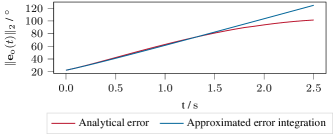
Figure 3: Comparison of the orientation path error computations. The reference and the current orientation path are computed over a time interval of $2.5\text{\,}\mathrm{s}$ using the constant angular velocities $\bm{\omega}_{\mathrm{r}}$ and $\bm{\omega}_{\mathrm{c}}$. The true evolution of the norm of eq. 26 in red is compared to the approximate computation of the norm according to eq. 30 in blue.

4.4.4 Orientation Path Error Decomposition

The orientation path error is decomposed similarly to the position path error. The rotation path error matrix $\mathbf{R}^{\mathrm{e}}=\text{Exp}(\mathbf{e}_{\mathrm{o}})$ consists of the orthogonal path errors $\mathbf{R}^{\bot,1}$ and $\mathbf{R}^{\bot,2}$ as well as the tangential path error $\mathbf{R}^{||}$, given by

$$\mathbf{R}^{\mathrm{e}}=\mathbf{R}^{\bot,2}\mathbf{R}^{||}\mathbf{R}^{\bot,1}=\mathbf{R}_{\mathrm{c}}\mathbf{R}_{\mathrm{r}}^{\mathrm{T}}\text{~{},}$$ (31)

with

$$\mathbf{R}^{\bot,1} =\text{Exp}(\mathbf{e}_{\mathrm{o}}^{\bot,1})=\text{Exp}(\alpha\mathbf{b}_{\mathrm{o,1}})$$ (32a)

$$\mathbf{R}^{||} =\text{Exp}(\mathbf{e}_{\mathrm{o}}^{||})=\text{Exp}(\beta\bm{\omega}_{\mathrm{r}})$$ (32b)

$$\mathbf{R}^{\bot,2} =\text{Exp}(\mathbf{e}_{\mathrm{o}}^{\bot,2})=\text{Exp}(\gamma\mathbf{b}_{\mathrm{o,2}})$$ (32c)

and the orthonormal orientation axes $\mathbf{b}_{\mathrm{o,1}}$, $\mathbf{b}_{\mathrm{o,2}}$, and $\bm{\omega}_{\mathrm{r}}$. The basis vectors $\mathbf{b}_{\mathrm{o,1}}$ and $\mathbf{b}_{\mathrm{o,2}}$ are obtained by following the procedure of the position path error in eq. 25 with the angular velocity $\bm{\omega}_{\mathrm{r}}$ instead of the Cartesian velocity $\mathbf{v}_{\mathrm{r}}$ and with the desired basis vector $\mathbf{b}_{\mathrm{o,d}}$. In this work, the projection of the error rotation matrix $\mathbf{R}^{\mathrm{e}}$ onto the orientation axes $\mathbf{b}_{\mathrm{o,1}}$, $\mathbf{b}_{\mathrm{o,2}}$, and $\bm{\omega}_{\mathrm{r}}$ is defined as

$$\operatorname*{arg\,min}_{\alpha,\beta,\gamma}\lVert\text{Log}(\mathbf{R}^{\mathrm{e}}\left(\mathbf{R}^{\bot,1}\right)^{\mathrm{T}}\bigl{(}\mathbf{R}^{||}\bigl{)}^{\mathrm{T}}\left(\mathbf{R}^{\bot,2}\right)^{\mathrm{T}})\rVert_{2}\text{~{},}$$ (33)

which gives the optimal values $\alpha^{*}$, $\beta^{*}$, and $\gamma^{*}$ that minimize the deviation from $\mathbf{R}^{\mathrm{e}}$. Note that this formulation is equivalent to roll, pitch, and yaw (RPY) angles, when $\mathbf{b}_{\mathrm{o,1}}$, $\mathbf{b}_{\mathrm{o,2}}$, and $\bm{\omega}_{\mathrm{r}}$ are the $z$, $x$ and $y$ axes, respectively [35]. Thus, solving  eq. 33 efficiently is done by computing the RPY angles for

$$\mathbf{R}_{\mathrm{RPY}}=\left(\mathbf{R}_{\mathrm{RPY}}^{\mathrm{e}}\right)^{\mathrm{T}}\mathbf{R}^{\mathrm{e}}\mathbf{R}_{\mathrm{RPY}}^{\mathrm{e}}\text{~{},}$$ (34)

with

$$\mathbf{R}_{\mathrm{RPY}}^{\mathrm{e}}=\left[\begin{array}[]{c|c|c}\mathbf{b}_{\mathrm{o,2}}&\bm{\omega}_{\mathrm{r}}&\mathbf{b}_{\mathrm{o,1}}\end{array}\right]$$ (35)

as the rotation matrix between the axes for the RPY angles and the desired axes for the error computation. The RPY representation has singularities when $\beta$ becomes $90\text{\,}\mathrm{\SIUnitSymbolDegree}$ or $270\text{\,}\mathrm{\SIUnitSymbolDegree}$ [35]. In this work, the tangential orientation path error $\mathbf{R}^{||}$ is minimized, as will be shown in section 4.5. Thus, the singularities are avoided by letting $\mathbf{R}^{||}$ represent the pitch angle $\beta$ and minimizing it, which also explains the order of the matrix multiplication in eq. 31.

Using the Lie representation and the approximation eq. 17, the optimization problem eq. 33 can be written as

$$\operatorname*{arg\,min}_{\alpha,\beta,\gamma}\lVert\mathbf{e}_{\mathrm{o}} -\gamma\mathbf{J}_{\mathrm{r}}^{-1}(\text{Log}(\mathbf{R}^{\mathrm{e}}\left(\mathbf{R}^{\bot,1}\right)^{\mathrm{T}}\bigl{(}\mathbf{R}^{||}\bigl{)}^{\mathrm{T}}))\mathbf{b}_{\mathrm{o,2}}$$ (36)

$$-\beta\mathbf{J}_{\mathrm{r}}^{-1}(\text{Log}(\mathbf{R}^{\mathrm{e}}\left(\mathbf{R}^{\bot,1}\right)^{\mathrm{T}}))\bm{\omega}_{\mathrm{r}}$$

$$-\alpha\mathbf{J}_{\mathrm{r}}^{-1}(\text{Log}(\mathbf{R}^{\mathrm{e}}))\mathbf{b}_{\mathrm{o,1}}\rVert_{2}\text{~{}.}$$

The Jacobians are not independent of the optimization variables $\alpha$, $\beta$, and $\gamma$, which makes solving eq. 36 a challenging task. To further simplify the problem it is assumed for the Jacobians that the optimal values $\alpha^{*}$, $\beta^{*}$, and $\gamma^{*}$ are close to an initial guess $\alpha^{0}$, $\beta^{0}$, and $\gamma^{0}$. This motivates to compute the Jacobians only for the initial guess to obtain the vectors

$$\mathbf{r}_{1} =\mathbf{J}_{\mathrm{r}}^{-1}(\text{Log}(\mathbf{R}^{\mathrm{e}}))\mathbf{b}_{\mathrm{o,1}}$$ (37a)

$$\mathbf{r}_{2} =\mathbf{J}_{\mathrm{r}}^{-1}(\text{Log}(\mathbf{R}^{\mathrm{e}}\left(\mathbf{R}^{\bot,1}(\alpha^{0})\right)^{\mathrm{T}}))\bm{\omega}_{\mathrm{r}}$$ (37b)

$$\mathbf{r}_{3} =\mathbf{J}_{\mathrm{r}}^{-1}(\text{Log}(\mathbf{R}^{\mathrm{e}}\left(\mathbf{R}^{\bot,1}(\alpha^{0})\right)^{\mathrm{T}}\bigl{(}\mathbf{R}^{||}(\beta^{0})\bigl{)}^{\mathrm{T}}))\mathbf{b}_{\mathrm{o,2}}\text{~{},}$$ (37c)

which are constant in the optimization problem eq. 36. Using eq. 37 in eq. 36 results in a quadratic program, and the optimal solution $\alpha^{*}$, $\beta^{*}$, and $\gamma^{*}$ can be obtained from

$$\begin{bmatrix}\mathbf{r}_{1}^{\mathrm{T}}\mathbf{r}_{1}&\mathbf{r}_{1}^{\mathrm{T}}\mathbf{r}_{2}&\mathbf{r}_{1}^{\mathrm{T}}\mathbf{r}_{3}\\ \mathbf{r}_{2}^{\mathrm{T}}\mathbf{r}_{1}&\mathbf{r}_{2}^{\mathrm{T}}\mathbf{r}_{2}&\mathbf{r}_{2}^{\mathrm{T}}\mathbf{r}_{3}\\ \mathbf{r}_{3}^{\mathrm{T}}\mathbf{r}_{1}&\mathbf{r}_{3}^{\mathrm{T}}\mathbf{r}_{2}&\mathbf{r}_{3}^{\mathrm{T}}\mathbf{r}_{3}\\ \end{bmatrix}\begin{bmatrix}\alpha\\ \beta\\ \gamma\end{bmatrix}=\begin{bmatrix}\mathbf{e}_{\mathrm{o}}^{\mathrm{T}}\mathbf{r}_{1}\\ \mathbf{e}_{\mathrm{o}}^{\mathrm{T}}\mathbf{r}_{2}\\ \mathbf{e}_{\mathrm{o}}^{\mathrm{T}}\mathbf{r}_{3}\end{bmatrix}$$ (38)

yielding

$$\alpha^{*}\approx\bm{\rho}_{\alpha}^{\mathrm{T}}(\mathbf{b}_{\mathrm{o,1}},\mathbf{b}_{\mathrm{o,2}},\bm{\omega}_{\mathrm{r}})\mathbf{e}_{\mathrm{o}}$$ (39a)

$$\beta^{*}\approx\bm{\rho}_{\beta}^{\mathrm{T}}(\mathbf{b}_{\mathrm{o,1}},\mathbf{b}_{\mathrm{o,2}},\bm{\omega}_{\mathrm{r}})\mathbf{e}_{\mathrm{o}}$$ (39b)

$$\gamma^{*}\approx\bm{\rho}_{\gamma}^{\mathrm{T}}(\mathbf{b}_{\mathrm{o,1}},\mathbf{b}_{\mathrm{o,2}},\bm{\omega}_{\mathrm{r}})\mathbf{e}_{\mathrm{o}}$$ (39c)

as the approximate optimal solution of eq. 33 with the solution vectors $\bm{\rho}_{\alpha}$, $\bm{\rho}_{\beta}$, and $\bm{\rho}_{\gamma}$, which are not given explicitly here.

Equation eq. 39 provides the approximate solution to eq. 33 at one point in time but the vectors $\mathbf{b}_{\mathrm{o,1}}$, $\mathbf{b}_{\mathrm{o,2}}$, and $\bm{\omega}_{\mathrm{r}}$ change along the path. It is possible to use the approximate solution eq. 39 to compute the optimal values for $\alpha^{*}$, $\beta^{*}$, and $\gamma^{*}$ at each time step when the robot's end effector traverses the path. However, the quality of the approximation in eq. 39 decreases when $\alpha$, $\beta$, and $\gamma$ grow. For the model predictive control formulation in section 4.5, the orientation path errors $\mathbf{e}_{\mathrm{o}}^{\bot,1}(t)$, $\mathbf{e}_{\mathrm{o}}^{\bot,2}(t)$, and $\mathbf{e}_{\mathrm{o}}^{||}(t)$ are computed over a time horizon spanning from $t_{0}$ to $t_{1}$. This motivates to obtain an initial guess $\alpha^{0}$, $\beta^{0}$, and $\gamma^{0}$ using eq. 33 at the time $t_{0}$ and then use the change of the approximate solution eq. 39 to propagate it over the time horizon. Thus, the time evolution of the errors are computed as

$$\mathbf{e}_{\mathrm{o}}^{\bot,1}(t)=\; \mathbf{e}_{\mathrm{o}}^{\bot,1}(t_{0})+\int_{t_{0}}^{t}\dot{\mathbf{e}}_{\mathrm{o}}^{\bot,1}(\tau)\text{d}\tau$$ (40a)

$$\mathbf{e}_{\mathrm{o}}^{\bot,2}(t)=\; \mathbf{e}_{\mathrm{o}}^{\bot,2}(t_{0})+\int_{t_{0}}^{t}\dot{\mathbf{e}}_{\mathrm{o}}^{\bot,2}(\tau)\text{d}\tau$$ (40b)

$$\mathbf{e}_{\mathrm{o}}^{||}(t)=\; \mathbf{e}_{\mathrm{o}}^{||}(t_{0})+\int_{t_{0}}^{t}\dot{\mathbf{e}}_{\mathrm{o}}^{||}(\tau)\text{d}\tau\text{~{},}$$ (40c)

where the initial guesses for $\alpha^{0}$, $\gamma^{0}$, and $\beta^{0}$ are used to compute the initial orientation path errors $\mathbf{e}_{\mathrm{o}}^{\bot,1}(t_{0})$, $\mathbf{e}_{\mathrm{o}}^{\bot,2}(t_{0})$, and $\mathbf{e}_{\mathrm{o}}^{||}(t_{0})$, respectively, meaning that eq. 40 is an approximation around the initial solution at time $t_{0}$. The time derivatives $\dot{\mathbf{e}}_{\mathrm{o}}^{\bot,1}$, $\dot{\mathbf{e}}_{\mathrm{o}}^{\bot,2}$, and $\dot{\mathbf{e}}_{\mathrm{o}}^{||}$ required in eq. 40 are computed using eq. 39

$$\begin{split}\dot{\mathbf{e}}_{\mathrm{o}}^{||}=\;&(\dot{\bm{\rho}}_{\beta}^{\mathrm{T}}(\mathbf{b}_{\mathrm{o,1}},\mathbf{b}_{\mathrm{o,2}},\bm{\omega}_{\mathrm{r}})\mathbf{e}_{\mathrm{o}}(t))\bm{\omega}_{\mathrm{r}}(\phi(t))\\ &+(\bm{\rho}_{\beta}^{\mathrm{T}}(\mathbf{b}_{\mathrm{o,1}},\mathbf{b}_{\mathrm{o,2}},\bm{\omega}_{\mathrm{r}})\dot{\mathbf{e}}_{\mathrm{o}}(t))\bm{\omega}_{\mathrm{r}}(\phi(t))\\ &+(\bm{\rho}_{\beta}^{\mathrm{T}}(\mathbf{b}_{\mathrm{o,1}},\mathbf{b}_{\mathrm{o,2}},\bm{\omega}_{\mathrm{r}})\mathbf{e}_{\mathrm{o}}(t))\bm{\omega}^{\prime}_{\mathrm{r}}(\phi(t))\dot{\phi}(t)\\ =\;&\dot{\mathbf{e}}_{\mathrm{o,proj}}(\bm{\rho}_{\beta}(\mathbf{b}_{\mathrm{o,1}},\mathbf{b}_{\mathrm{o,2}},\bm{\omega}_{\mathrm{r}}),\bm{\omega}_{\mathrm{r}})\end{split}$$ (41a)

$$\dot{\mathbf{e}}_{\mathrm{o}}^{\bot,1}=\; \dot{\mathbf{e}}_{\mathrm{o,proj}}(\bm{\rho}_{\alpha}(\mathbf{b}_{\mathrm{o,1}},\mathbf{b}_{\mathrm{o,2}},\bm{\omega}_{\mathrm{r}}),\mathbf{b}_{\mathrm{o,1}})$$ (41b)

$$\dot{\mathbf{e}}_{\mathrm{o}}^{\bot,2}=\; \dot{\mathbf{e}}_{\mathrm{o,proj}}(\bm{\rho}_{\gamma}(\mathbf{b}_{\mathrm{o,1}},\mathbf{b}_{\mathrm{o,2}},\bm{\omega}_{\mathrm{r}}),\mathbf{b}_{\mathrm{o,2}})\text{~{}.}$$ (41c)

Thus, the approximation error of eq. 40 is limited to the change of the orientation path errors within the time horizon of the MPC.

The orthogonal orientation path errors $\mathbf{e}_{\mathrm{o}}^{\bot,1}$ and $\mathbf{e}_{\mathrm{o}}^{\bot,2}$ are represented similar to eq. 24 by

$$\mathbf{e}_{\mathrm{o,\mathrm{proj}}}^{\bot} =\begin{bmatrix}e_{\mathrm{o,\mathrm{proj},1}}^{\bot}\\ e_{\mathrm{o,\mathrm{proj},2}}^{\bot}\end{bmatrix}=\begin{bmatrix}\alpha\\ \gamma\end{bmatrix}\text{~{},}$$ (42)

in the orthogonal error plane.

Remark.

Due to the iterative computation of the orientation path errors in eq. 40, the reference path $\bm{\pi}_{\mathrm{o}}(\phi(t))$ is only evaluated at the initial time $t_{0}$. For all other time points in the time horizon from $t_{0}$ to $t_{1}$, only the reference angular velocity $\bm{\omega}_{\mathrm{r}}(\phi(t))$ and its derivative $\bm{\omega}^{\prime}_{\mathrm{r}}(\phi(t))$ with respect to the path parameter $\phi$ are needed.

4.5 Optimization Problem

In this section, the results of the previous sections are utilized to formulate the optimal control problem for the proposed MPC framework. The goal is to follow a desired reference path of the Cartesian end-effector's position and orientation within given asymmetric error bounds in the error plane orthogonal to the path, which also includes compliance with desired via-points. At the same time, the system dynamics of the controlled robot eq. 6 and the state and input constraints must be satisfied. To govern the progress along the path, the discrete-time path-parameter dynamics

$$\bm{\xi}_{k+1}=\mathbf{\Phi}_{\xi}\bm{\xi}_{k}+\mathbf{\Gamma}_{0,\xi}v_{k}+\mathbf{\Gamma}_{1,\xi}v_{k+1}$$ (43)

are introduced, with the state $\bm{\xi}_{k}^{\mathrm{T}}=[\phi_{k},\dot{\phi}_{k},\ddot{\phi}_{k}]$ and the input $v_{k}={\mathop{\kern 0.0pt\phi}\limits^{\makebox[0.0pt][c]{\vbox to-1.4pt{\kern-2.0pt\hbox{...}\vss}}}}_{k}$. The linear system eq. 43 is chosen to have the same order as eq. 6 and also uses hat functions for the interpolation of the jerk input ${\mathop{\kern 0.0pt\phi}\limits^{\makebox[0.0pt][c]{\vbox to-1.4pt{\kern-2.0pt\hbox{...}\vss}}}}_{k}$. Thus, the optimization problem for the MPC is formulated as

$$\min_{\begin{subarray}{c}\mathbf{u}_{1},\ldots,\mathbf{u}_{N},\\ \mathbf{x}_{1},\ldots,\mathbf{x}_{N},\\ \bm{\xi}_{1},\ldots,\bm{\xi}_{N},\\ v_{1},\ldots,v_{N}\end{subarray}} \sum_{i=1}^{N}l(\mathbf{x}_{i},\bm{\xi}_{i},\mathbf{u}_{i},v_{i})$$ (44a)

$$\text{s.t.\quad}\begin{split}\mathbf{x}_{i+1}=\mathbf{\Phi}\mathbf{x}_{i}+\mathbf{\Gamma}_{0}\mathbf{u}_{i}+&\mathbf{\Gamma}_{1}\mathbf{u}_{i+1}\text{,}\\ &i=0,\ldots,N-1\\ \end{split}$$ (44b)

$$\begin{split}\bm{\xi}_{i+1}=\mathbf{\Phi}_{\xi}\bm{\xi}_{i}+\mathbf{\Gamma}_{0,\xi}v_{i}&+\mathbf{\Gamma}_{1,\xi}v_{i+1}\text{,}\\ &i=0,\ldots,N-1\\ \end{split}$$ (44c)

$$\mathbf{x}_{0}=\mathbf{x}_{\mathrm{init}}$$ (44d)

$$\mathbf{u}_{0}=\mathbf{u}_{\mathrm{init}}$$ (44e)

$$\bm{\xi}_{0}=\bm{\xi}_{\mathrm{init}}$$ (44f)

$$v_{0}=v_{\mathrm{init}}$$ (44g)

$$\underline{\mathbf{x}}\leq\mathbf{x}_{i+1}\leq\overline{\mathbf{x}}$$ (44h)

$$\underline{\mathbf{u}}\leq\mathbf{u}_{i+1}\leq\overline{\mathbf{u}}$$ (44i)

$$\phi_{i+1}\leq\phi_{\mathrm{f}}$$ (44j)

$$0\leq\dot{\phi}_{i+1}$$ (44k)

$$\psi_{\mathrm{p},m}(\mathbf{e}^{\bot}_{\mathrm{p},\mathrm{proj},i+1})\leq 0\text{~{},}\quad m=1,2$$ (44l)

$$\psi_{\mathrm{o},m}(\mathbf{e}^{\bot}_{\mathrm{o},\mathrm{proj},i+1})\leq 0\text{~{},}\quad m=1,2\text{~{}.}$$ (44m)

The quantities $\mathbf{x}_{\mathrm{init}}$, $\mathbf{u}_{\mathrm{init}}$, $\bm{\xi}_{\mathrm{init}}$, and $v_{\mathrm{init}}$ in eq. 44d-eq. 44g describe the initial conditions at the initial time $t_{0}$. In eq. 44h and eq. 44i, the system states $\mathbf{x}$ and the inputs $\mathbf{u}$ are bounded from below and above with the corresponding limits $\underline{\mathbf{x}}$, $\overline{\mathbf{x}}$, $\underline{\mathbf{u}}$, and $\overline{\mathbf{u}}$. The path parameter never exceeds the maximum value $\phi_{\mathrm{f}}$, see eq. 44j, and always progresses $0\leq\dot{\phi}_{i+1}$, see eq. 44k. In eq. 44l and eq. 44m, the Cartesian orthogonal position and orientation path errors are bounded by the constraint functions $\psi_{\mathrm{p},m}$ and $\psi_{\mathrm{o},m}$ in both desired basis vector directions, which is further detailed in section 5. The position reference path is given by

$$\bm{\pi}_{\mathrm{p},i}=\bm{\pi}_{\mathrm{p}}(\phi_{i})$$ (45)

for each discrete time instance $t_{0}+iT_{\mathrm{s}}$. An explicit representation of $\bm{\pi}_{\mathrm{o}}(\phi(t))$ is not required within the optimization problem eq. 44, as discussed in section 4.4.4. The objective function eq. 44a,

$$l\left(\mathbf{x}_{i},\bm{\xi}_{i},\mathbf{u}_{i},v_{i}\right) =w_{||}\left(\lVert\mathbf{e}_{\mathrm{p},i}^{||}\rVert_{2}^{2}+\lVert\mathbf{e}^{||}_{\mathrm{o},i}\rVert_{2}^{2}\right)$$ (46)

$$+w_{\dot{e}}\Bigl{(}\lVert\dot{\mathbf{e}}_{\mathrm{p},i}\rVert_{2}^{2}+\lVert\dot{\mathbf{e}}_{\mathrm{o},i}\rVert_{2}^{2}\Bigl{)}+\lVert\bm{\xi}_{i}-\bm{\xi}_{\mathrm{d}}\rVert_{\mathbf{W}_{\xi}}^{2}$$

$$+w_{\mathrm{n}}\lVert\mathbf{P}_{\mathrm{n,0}}\dot{\mathbf{q}}_{\mathrm{d}}\rVert_{2}^{2}+w_{\mathrm{u}}\lVert\mathbf{u}_{i}\rVert_{2}^{2}+w_{\mathrm{v}}\lVert v_{i}\rVert_{2}^{2}\text{~{},}$$

minimizes the tangential position and orientation path errors with the tangential error weight $w_{||}>0$. Small tangential error norms $\lVert\mathbf{e}_{\mathrm{p},i}^{||}\rVert_{2}^{2}$ and $\lVert\mathbf{e}_{\mathrm{o},i}^{||}\rVert_{2}^{2}$ are ensured when choosing $w_{||}$ sufficiently large. The path error velocity term $\lVert\dot{\mathbf{e}}_{\mathrm{p},i}\rVert_{2}^{2}+\lVert\dot{\mathbf{e}}_{\mathrm{o},i}\rVert_{2}^{2}$, with the weight $w_{\dot{e}}>0$, brings damping into the path error systems. The term $\lVert\bm{\xi}_{i}-\bm{\xi}_{\mathrm{d}}\rVert_{\mathbf{W}_{\xi}}^{2}=(\bm{\xi}_{i}-\bm{\xi}_{\mathrm{d}})^{\mathrm{T}}\mathbf{W}_{\xi}(\bm{\xi}_{i}-\bm{\xi}_{\mathrm{d}})$, with the positive definite weighting matrix $\mathbf{W}_{\xi}$, makes the state $\bm{\xi}$ of the path-parameter system eq. 44c approach the desired state $\bm{\xi}_{\mathrm{d}}=[\phi_{\mathrm{f}},0,0]^{\mathrm{T}}$. Movement in the joint nullspace is minimized using the term $w_{\mathrm{n}}\lVert\mathbf{P}_{\mathrm{n,0}}\dot{\mathbf{q}}_{\mathrm{d}}\rVert_{2}^{2}$, $w_{\mathrm{n}}>0$, with the constant projection matrix $\mathbf{P}_{\mathrm{n,0}}=\mathbf{P}_{\mathrm{n}}(\mathbf{q}_{\mathrm{d},0})$. The last two terms in eq. 46, with the weights $w_{\mathrm{u}}>0$, $w_{\mathrm{v}}>0$, serve as regularization terms.

Within the MPC, the planning problem eq. 44 is solved at each time step with the same sampling time $T_{\mathrm{s}}$. Each step, the optimal control inputs $\mathbf{u}_{i}$ and $v_{i}$ are computed over the horizon $i=1,\ldots,N$, but only the first control inputs $\mathbf{u}_{1}$ and $v_{1}$ are applied to the system.

5 Orthogonal Path Error Bounds

To stay within predefined error bounds, the MPC formulation eq. 44 bounds the orthogonal position and orientation path errors in eq. 44l and eq. 44m. The bounds are specified in the Cartesian space and allow for meaningful interpretations, which can be advantageously used, e.g., for tasks in cluttered environments. The formulation of the constraint functions is detailed in this section. First, the case of symmetric path error bounds is examined and then generalized to asymmetric error bounds with respect to the desired basis vector directions to increase the flexibility of the method. The resulting bounds are visualized for one position basis direction in fig. 4.

5.1 Symmetric Bounds

For a symmetric bounding of the orthogonal path errors, the representations $\mathbf{e}_{\mathrm{p,proj}}^{\bot}$, given in eq. 24, and $\mathbf{e}_{\mathrm{o,proj}}^{\bot}$, given in eq. 42, are used. Thus, the error bounding constraints

$$\psi_{j,m}^{\mathrm{sym}}(\mathbf{e}_{j,\mathrm{proj}}^{\bot})=\left(e_{j,\mathrm{proj},m}^{\bot}\right)^{2}-\left(\Upsilon_{j,m}(\phi)\right)^{2}\leq 0\text{~{},}$$ (47)

with the bounding functions $\Upsilon_{j,m}(\phi)$, define symmetric box constraints centered on the reference path. The index $j\in\{\mathrm{p,o}\}$ indicates the position and orientation error, and the index $m=1,2$ refers to the basis vector direction, leading to four constraints in total.

The bounding functions $\Upsilon_{j,m}(\phi)$ are used to smoothly vary the error bounds such that no orthogonal path errors are allowed at the via-points but deviations from the path are possible in between the via-points depending on the respective task and situation. Let us assume that two via-points exist at the path points $\phi_{l}$ and $\phi_{l+1}$. In this work, the bounding functions for $\phi_{l}\leq\phi\leq\phi_{l+1}$ are chosen as fourth-order polynomials. They provide sufficient smoothness and are easy to specify by using the conditions

$$\Upsilon_{j,m}(\phi_{l}) =0$$ (48a)

$$\Upsilon_{j,m}(\phi_{l+1}) =0$$ (48b)

$$\Upsilon_{j,m}^{\prime}(\phi_{l}) =s_{0}$$ (48c)

$$\Upsilon_{j,m}^{\prime}(\phi_{l+1}) =s_{\mathrm{f}}$$ (48d)

$$\Upsilon_{j,m}\left(\frac{\phi_{l}+\phi_{l+1}}{2}\right) =\Upsilon_{j,\mathrm{max}}\text{~{},}$$ (48e)

where the design parameters are $s_{0}$, $s_{\mathrm{f}}$, and $\Upsilon_{j,\mathrm{max}}$. Note that in general, any sufficiently smooth function can be used to bound the orthogonal path errors. For multiple via-points, the error bounding functions are defined for each segment between the via-points, meaning that $L$ via-points lead to $L-1$ segments with four bounding functions each. The case of two segments in 2D is visualized in fig. 4.

Remark.

The error bounding functions $\Upsilon_{j,m}(\phi)$ depend on the path parameter $\phi$ meaning that the orthogonal error is only correctly bounded as long as the tangential errors $\mathbf{e}_{\mathrm{p}}^{||}$ and $\mathbf{e}_{\mathrm{o}}^{||}$ are close to zero. This assumption holds true if the weight $w_{||}$ in eq. 46 is sufficiently large compared to the other weights.

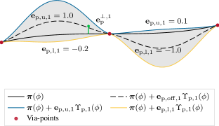
Figure 4: 2D Visualization of a position reference path $\bm{\pi}_{\mathrm{p}}(\phi)$ with error bounds. The symmetric error bounding functions $\Upsilon_{\mathrm{p,1}}$ are adapted by the upper and lower bounds $\mathbf{e}_{\mathrm{p,u,1}}$ and $\mathbf{e}_{\mathrm{p,l,1}}$ to asymmetrically bound the orthogonal position path error $\mathbf{e}^{\bot,1}_{\mathrm{p}}$. The shaded gray regions indicate the area where $\psi_{\mathrm{p,1}}(\mathbf{e}_{\mathrm{p,proj}}^{\bot})\leq 0$. The error bounding functions $\Upsilon_{\mathrm{p,1}}$ and the upper and lower bounds $\mathbf{e}_{\mathrm{p,u,1}}$ and $\mathbf{e}_{\mathrm{p,l,1}}$ are defined for both segments between the three shown via-points.

5.2 Asymmetric Bounds

The symmetric error bounds from the previous section are generalized in this section to allow for asymmetric bounds around the reference paths. The formulation

$$\psi_{j,m}(\mathbf{e}_{j,\mathrm{proj}}^{\bot})\leq 0\text{~{},}\quad j\in\{\mathrm{p,o}\},\quad m=1,2\text{~{},}$$ (49)

with

$$\psi_{j,m}(\mathbf{e}_{j,\mathrm{proj}}^{\bot})=\left(e_{j,\mathrm{proj},m}^{\bot}-e_{j,\mathrm{off},m}\right)^{2}-\lambda_{j,m}^{2}\text{~{},}$$ (50)

generalizes eq. 47 and is used in this work. The offsets $e_{j,\mathrm{off},m}=\frac{1}{2}\left(e_{j,\mathrm{l},m}+e_{j,\mathrm{u},m}\right)\Upsilon_{j,m}$ and the bounds $\lambda_{j,m}=\frac{1}{2}(e_{j,\mathrm{u},m}-e_{j,\mathrm{l},m})\Upsilon_{j,m}$ are parametrized using the upper and lower bounds $\mathbf{e}_{j,\mathrm{u}}^{\mathrm{T}}=[e_{j,\mathrm{u},1},e_{j,\mathrm{u},2}]$ and $\mathbf{e}_{j,\mathrm{l}}^{\mathrm{T}}=[e_{j,\mathrm{l},1},e_{j,\mathrm{l},2}]$, referred to with the index $\mathrm{u}$ and $\mathrm{l}$, respectively, and the bounding functions $\Upsilon_{j,m}$ from section 5.1. Note that choosing $e_{j,\mathrm{u},m}=1$ and $e_{j,\mathrm{l},m}=-1$ reduces eq. 50 to the symmetric case eq. 47. Intuitively, the upper and lower bounds $e_{j,\mathrm{u},m}$ and $e_{j,\mathrm{l},m}$ define how much of the bound, defined by $\Upsilon_{j,m}$, can be used by the MPC to deviate in orthogonal direction from the reference path. For example, setting $e_{\mathrm{p,l},1}=-0.5$ means that the orthogonal position path error can only deviate $50\text{\,}\mathrm{\char 37\relax}$ of the bounding function $\Upsilon_{\mathrm{p,1}}$ in the negative direction defined by the basis vector $\mathbf{b}_{\mathrm{p},1}$. A 2D example is given in fig. 4.

Remark.

Setting $\Upsilon_{j,m}(\phi_{l})=0$ and $\Upsilon_{j,m}(\phi_{l+1})=0$ in eq. 48 may lead to numerical issues in the MPC eq. 44. This is especially true for the orientation path error bounds as the orientation errors are only approximated. Therefore, relaxations $\Upsilon_{j,m}(\phi_{l})=\epsilon_{l}>0$ and $\Upsilon_{j,m}(\phi_{l+1})=\epsilon_{l+1}>0$ are used in practice. Note that in combination with asymmetric error bounds, this may entail discontinuous error bounds at the via-points. Choosing linearly varying upper and lower bounds $\mathbf{e}_{j,\mathrm{u}}^{\mathrm{T}}$ and $\mathbf{e}_{j,\mathrm{l}}^{\mathrm{T}}$ fixes these issues but is not further detailed here.

6 BoundMPC with Linear Reference Paths

Figure 5: Visualization of a linear reference path. The current position along the path is $\bm{\pi}_{\mathrm{p}}(\phi(t))$ on the first linear segment.

This section describes the application of the proposed MPC framework to piecewise linear reference paths. This is a special case of the above formulation yielding beneficial simplifications of the involved terms and expressions. Additionally, admissible piecewise linear reference paths can be easily generated by just specifying via-points. This way, the reference path is defined by points to be passed with the robot's end effector, and the realized trajectory between the points is computed by the proposed MPC framework respecting the given bounds and the system dynamics. For obstacle avoidance, linear paths with Cartesian error bounds allow for a simple and accurate formulation of the collision-free space. Moreover, arc-length parametrization becomes trivial for linear paths. In this section, piecewise linear reference paths are introduced and the simplifications that follow from using such paths are derived.

6.1 Reference Path Formulation

In this work, a piecewise linear reference path is a sequence of $L$ linear segments, i.e.

$$\bm{\pi}_{\mathrm{p}}(\phi)=\begin{cases}\bm{\pi}_{\mathrm{p,0}}(\phi)&\phi_{0}\leq\phi<\phi_{1}\\ \bm{\pi}_{\mathrm{p,1}}(\phi)&\phi_{1}\leq\phi<\phi_{2}\\ \quad\vdots\\ \bm{\pi}_{\mathrm{p},L-1}(\phi)&\phi_{L-1}\leq\phi<\phi_{L}\end{cases}$$ (51)

for the position reference path $\bm{\pi}_{\mathrm{p}}(\phi)$. The values $\phi_{l}$, $l=0,\ldots,L$, indicate the locations of the via-points along the path, where $\phi_{0}$ refers to the starting and $\phi_{L}$ to the terminal point. In fig. 5, an example of two linear position reference segments is visualized. Each segment of the reference position path is parameterized by the slope $\mathbf{m}_{l}$ of unit length and the position $\mathbf{b}_{l}$ at the via-point

$$\bm{\pi}_{\mathrm{p},l}(\phi)=\mathbf{m}_{l}(\phi-\phi_{l})+\mathbf{b}_{l}\text{~{},}$$ (52)

with the arc-length parameter $\phi$. To ensure continuity of $\bm{\pi}_{\mathrm{p}}(\phi)$, the following condition must hold

$$\mathbf{b}_{l+1}=\mathbf{m}_{l}(\phi_{l+1}-\phi_{l})+\mathbf{b}_{l}\text{~{}.}$$ (53)

Thus, the path eq. 51 is uniquely defined by the via-points $\mathbf{b}_{l}$ $l=0,\ldots,L$.

The orientation reference path $\bm{\pi}_{\mathrm{o}}(\phi)$ is formulated analogously. Here it is assumed that the angular reference velocity $\bm{\omega}_{\mathrm{r},l}$ between two via-points $l$ and $l+1$ is constant. Then the path segments $\bm{\pi}_{\mathrm{o},l}(\phi)$ read as

$$\bm{\pi}_{\mathrm{o},l}(\phi) =\text{Log}(\text{Exp}(\bm{\omega}_{\mathrm{r},l}(\phi-\phi_{l}))\mathbf{R}_{l})\text{~{},~{}}l=0,\ldots,L-1\text{~{},}$$ (54)

where $\mathbf{R}_{l}$ is the end-effector's orientation at the via-point $l$. Moreover, the condition

$$\mathbf{R}_{l+1}=\text{Exp}(\bm{\omega}_{\mathrm{r},l}(\phi_{l+1}-\phi_{l}))\mathbf{R}_{l}$$ (55)

must be satisfied to ensure continuity of the piecewise linear orientation reference path $\bm{\pi}_{\mathrm{o}}(\phi)$.

The piecewise linear position reference path eq. 51 is used to compute the tangential and orthogonal position path errors for the optimal control problem eq. 44. As discussed in section 4.4.4, the orientation reference $\bm{\pi}_{\mathrm{o}}(\phi(t))$ is never explicitly used within the optimization problem eq. 44 due to the iterative computation of the orientation path errors in eq. 40. This is detailed for piecewise linear orientation reference paths in the next section.

Remark.

The orthonormal basis vectors $\mathbf{b}_{\mathrm{p,1}}$, $\mathbf{b}_{\mathrm{p,2}}$, $\mathbf{b}_{\mathrm{o,1}}$, and $\mathbf{b}_{\mathrm{o,2}}$ are constant for each linear segment and will be referred to as $\mathbf{b}_{\mathrm{p,1},l}$, $\mathbf{b}_{\mathrm{p,2},l}$, $\mathbf{b}_{\mathrm{o,1},l}$, and $\mathbf{b}_{\mathrm{o,2},l}$ with $l=0,\ldots,L-1$. Furthermore, the error bounding functions with the upper and lower bounds from section 5 are denoted as $\Upsilon_{j,m,l}$, $\mathbf{e}_{j,\mathrm{u},l}$, and $\mathbf{e}_{j,\mathrm{l},l}$, $j\in\{\mathrm{p,o}\}$, $m=1,2$, respectively.

Remark.

Sampling-based methods, such as RRT, can be applied to efficiently plan collision-free piecewise linear reference paths in the Cartesian space, which is simpler than generating admissible paths in the joint space. The proposed MPC framework is then employed to find the joint trajectories that follow the paths within the given bounds.

6.2 Computation of the Orientation Path Errors

In this section, the orientation path error computations are derived for the piecewise linear orientation reference paths introduced in eq. 54. Let us assume that the initial path parameter of the planner at the initial time $t_{0}$ is $\phi_{0}$. The current segment at time $t$ has the index $l_{t}$. The orientation path error eq. 30 is integrated in the form

$$\mathbf{e}_{\mathrm{o}}(t)= \mathbf{e}_{\mathrm{o}}(t_{0})+\mathbf{J}_{\mathrm{l}}^{-1}(\mathbf{e}_{\mathrm{o}}(t_{0}))\int_{t_{0}}^{t}\bm{\omega}_{\mathrm{c}}(\tau)\mathrm{d}\tau$$ (56)

$$-\mathbf{J}_{\mathrm{r}}^{-1}(\mathbf{e}_{\mathrm{o}}(t_{0}))\int_{\phi(t_{0})}^{\phi(t)}\bm{\omega}_{\mathrm{r}}(\sigma)\mathrm{d}\sigma$$

$$= \mathbf{e}_{\mathrm{o}}(t_{0})+\mathbf{J}_{\mathrm{l}}^{-1}(\mathbf{e}_{\mathrm{o}}(t_{0}))(\mathbf{\Omega}_{\mathrm{c}}(t)-\mathbf{\Omega}_{\mathrm{c}}(t_{0}))$$

$$-\mathbf{J}_{\mathrm{r}}^{-1}(\mathbf{e}_{\mathrm{o}}(t_{0}))(\mathbf{\Omega}_{\mathrm{r}}(\phi(t))-\cancelto{0}{\mathbf{\Omega}_{\mathrm{r}}(\phi_{0})})\text{~{},}$$

where $\mathbf{\Omega}_{\mathrm{c}}(t)$ and

$$\mathbf{\Omega}_{\mathrm{r}}(\phi(t))=\sum_{l=0}^{l_{t}-1}\bm{\omega}_{\mathrm{r},l}(\phi_{l+1}-\phi_{l})+\bm{\omega}_{\mathrm{r},l_{t}}(\phi(t)-\phi_{l_{t}})$$ (57)

are the integrated angular velocities of the current robot motion and the piecewise linear reference path, respectively. Numerical integration is used to obtain $\mathbf{\Omega}_{\mathrm{c}}(t)$. Due to the assumption on the initial value of $\phi(t)$, the term $\mathbf{\Omega}_{\mathrm{r}}(\phi_{0})$ vanishes. This formulation allows the representation of the current orientation path error $\mathbf{e}_{\mathrm{o}}(t)$ by the integrated angular velocities $\mathbf{\Omega}_{\mathrm{c}}(t)$ and $\mathbf{\Omega}_{\mathrm{r}}(\phi(t))$ and does not require the current orientation $\mathbf{R}_{\mathrm{c}}(t)$ or the current orientation reference path $\bm{\pi}_{\mathrm{o}}(\phi(t))$. For linear orientation reference paths, $\bm{\omega}_{\mathrm{r}}^{\prime}(\phi(t))=\mathbf{0}$ and $\bm{\rho}_{\beta}$ is constant, and the tangential orientation path error in eq. 40 becomes

$$\mathbf{e}_{\mathrm{o}}^{||}(t)= \mathbf{e}_{\mathrm{o}}^{||}(t_{0})+\int_{t_{0}}^{t}\left(\bm{\rho}_{\beta}^{\mathrm{T}}(\mathbf{b}_{\mathrm{o,1}},\mathbf{b}_{\mathrm{o,2}},\bm{\omega}_{\mathrm{r}})\dot{\mathbf{e}}_{\mathrm{o}}(\tau)\right)\bm{\omega}_{\mathrm{r}}(\phi(\tau))\text{d}\tau$$ (58)

$$= \mathbf{e}_{\mathrm{o}}^{||}(t_{0})+\sum_{l=0}^{l_{t}-1}\left(\bm{\rho}_{\beta,l}^{\mathrm{T}}(\mathbf{e}_{\mathrm{o}}(t_{\phi_{l+1}})-\mathbf{e}_{\mathrm{o}}(t_{\phi_{l}}))\right)\bm{\omega}_{\mathrm{r},l}$$

$$+\left(\bm{\rho}_{\beta,l_{t}}^{\mathrm{T}}(\mathbf{e}_{\mathrm{o}}(t)-\mathbf{e}_{\mathrm{o}}(t_{\phi_{l_{t}}}))\right)\bm{\omega}_{\mathrm{r},l_{t}}\text{~{},}$$

with

$$\bm{\rho}_{\beta,l}=\bm{\rho}_{\beta}(\mathbf{b}_{\mathrm{o,1},l},\mathbf{b}_{\mathrm{o,2},l},\bm{\omega}_{\mathrm{r},l})\text{~{},}$$ (59)

and the basis vectors $\mathbf{b}_{\mathrm{o,1},l}$ and $\mathbf{b}_{\mathrm{o,2},l}$ of the respective segment. Since the $t_{\phi_{l}}$ values (time associated with the path parameter $\phi_{l}$) in eq. 58 are unknown, they are approximated as the last discrete time stamp after $\phi_{l}$. Furthermore, the orthogonal orientation path errors $\mathbf{e}_{\mathrm{o}}^{\bot,1}$ and $\mathbf{e}_{\mathrm{o}}^{\bot,2}$ are computed analogously to eq. 58. Note that the values $\bm{\rho}_{\alpha,l}$, $\bm{\rho}_{\beta,l}$, and $\bm{\rho}_{\gamma,l}$, $l=0,\ldots,L-1$ are required for the optimization problem eq. 44. However, since they depend on values known prior to the optimization problem, they can be precomputed. The MPC using linear reference paths is further detailed in algorithm 1.

Algorithm 1 BoundMPC with linear reference paths

sampling time $T_{\mathrm{s}}$, reference paths $\bm{\pi}_{\mathrm{p}}$, $\bm{\pi}_{\mathrm{o}}$, initial states $\mathbf{x}_{\mathrm{init}}$, $\mathbf{u}_{\mathrm{init}}$, $\bm{\xi}_{\mathrm{init}}$, $v_{\mathrm{init}}$

$t\leftarrow t_{0}$

$\bm{\xi}^{\mathrm{T}}(t_{0})\leftarrow[0,0,0]$ $\triangleright$ Initialize state of path progress system

while $\phi(t)<\phi_{\mathrm{f}}$ do

     for $l=0,\ldots,L-1$ do $\triangleright$ For each linear segment

         obtain $\mathbf{m}_{l}$, $\bm{\omega}_{\mathrm{r},l}$, $\mathbf{b}_{l}$ $\triangleright$ Slopes and biases

         for $j=\mathrm{p,o}$ do $\triangleright$ For position and orientation

              obtain $\Upsilon_{j,1,l}$ and $\Upsilon_{j,2,l}$ $\triangleright$ Error bounds

              obtain $\mathbf{e}_{j,\mathrm{u},l}$ and $\mathbf{e}_{j,\mathrm{l},l}$

         end for

     end for

     compute $\mathbf{e}_{\mathrm{o}}(t_{0})$ using eq. 26 $\triangleright$ Initial orientation errors

     compute $\mathbf{e}_{\mathrm{o}}^{||}(t_{0})$, $\mathbf{e}_{\mathrm{o}}^{\bot,1}(t_{0})$, $\mathbf{e}_{\mathrm{o}}^{\bot,2}(t_{0})$ using eq. 33

     compute $\mathbf{J}_{\mathrm{l}}^{-1}(\mathbf{e}_{\mathrm{o}}(t_{0}))$, $\mathbf{J}_{\mathrm{r}}^{-1}(\mathbf{e}_{\mathrm{o}}(t_{0}))$ $\triangleright$ Jacobians

     for $l=0,\ldots,L-1$ do $\triangleright$ For each linear segment

         compute $\bm{\rho}_{\alpha,l}$, $\bm{\rho}_{\beta,l}$ and $\bm{\rho}_{\gamma,l}$ $\triangleright$ Projection vectors

     end for

     compute $\mathbf{P}_{\mathrm{n,0}}$ $\triangleright$ Nullspace projection matrix

     solve eq. 44 $\triangleright$ Optimization

     apply $\mathbf{u}_{1}$ to the robot

     $t=t+T_{\mathrm{s}}$ $\triangleright$ Increment time

     $\mathbf{x}_{\mathrm{init}}=\mathbf{x}_{1}$ $\triangleright$ Obtain new initial state

     $\mathbf{u}_{\mathrm{init}}=\mathbf{u}_{1}$

     $\bm{\xi}_{\mathrm{init}}=\bm{\xi}_{1}$

     $v_{\mathrm{init}}=v_{1}$

end while

7 Online Replanning

A major advantage using the proposed framework compared to state-of-the-art methods is the ability to replan a given path in real time during the motion of the robot in order to adapt to new goals or dynamic changes in the environment. Two different situations for replanning are possible based on when the reference path is adapted, i.e.

1. outside of the current MPC horizon

2. within the current MPC horizon.

The first situation is trivial since it does not affect the subsequent MPC iteration. More challenging is the second situation, which requires careful consideration on how to adapt the current reference path such that the optimization problem remains feasible. This situation is depicted for linear position reference paths in fig. 6 and applies similarly to linear orientation paths. In this figure, replanning takes place at the current path parameter $\phi$. The path adaptation is performed at the path parameter $\tilde{\phi}$ and the remaining arc length to react to this replanned path is $\tilde{\phi}-\phi$. Consequently, the new error bounds, parametrized by $\tilde{\Upsilon}_{\mathrm{p}}(\tilde{\phi})$, need to be chosen such that the optimization problem stays feasible, and it is advisable to relax the initial error bound $\tilde{\Upsilon}_{\mathrm{p}}(\tilde{\phi})$. This might lead to a suboptimal solution if the via-point cannot be reached exactly, as discussed in section 6, but it will keep the problem feasible. In this work, $\tilde{\Upsilon}_{\mathrm{p}}(\tilde{\phi})=\Upsilon_{\mathrm{p}}(\tilde{\phi})$ is used, which works well in practice. Note that this choice guarantees feasibility for the worst case scenario $\tilde{\phi}=\phi$ as long as the tangential path errors $\mathbf{e}_{\mathrm{p}}^{||}$ and $\mathbf{e}_{\mathrm{o}}^{||}$ are close to zero, which is enforced by a large weight $w_{||}$ in eq. 46. This is visualized in fig. 7, where is becomes clear that the new orthogonal path error always decreases during the replanning while the tangential path error increases, namely $\tilde{\mathbf{e}}_{\mathrm{p}}^{\bot}\leq\mathbf{e}_{\mathrm{p}}^{\bot}$ and $\tilde{\mathbf{e}}_{\mathrm{p}}^{||}\geq\mathbf{e}_{\mathrm{p}}^{||}$, which makes $\tilde{\Upsilon}_{\mathrm{p}}(\tilde{\phi})=\Upsilon_{\mathrm{p}}(\tilde{\phi})$ a conservative choice. This feasibility analysis does not consider the dynamics of the end effector.

Figure 6: Replanning for a linear position reference path. The blue color indicates the current state $\mathbf{p}_{\mathrm{c}}(t)$. The current reference point at time $t$ is $\bm{\pi}_{\mathrm{p}}(\phi)$. Replanning takes place at the current path parameter $\phi$ with the updated path deviating from the old reference at $\tilde{\phi}$ indicated in green. The error bound at this point is parametrized by $\Upsilon_{\mathrm{p}}(\tilde{\phi})$ for the old path and $\tilde{\Upsilon}_{\mathrm{p}}(\tilde{\phi})$ for the new path. This visualization analogously applies to orientation path replanning.

Figure 7: Path error changes during replanning. The blue color indicates the current state. The replanned path starts at the current path parameter $\phi$ indicated in green. The error bound at this point is parametrized by $\Upsilon_{\mathrm{p}}(\phi)$ for the old path and $\tilde{\Upsilon}_{\mathrm{p}}(\phi)$ for the new path such that $\Upsilon_{\mathrm{p}}(\phi)=\tilde{\Upsilon}_{\mathrm{p}}(\phi)$. It is assumed that the initial tangential path error $\mathbf{e}_{\mathrm{p}}^{||}\approx 0$.

8 Implementation Details

The proposed MPC is implemented on a Kuka LBR iiwa 14 R820 robot. For the optimization problem eq. 44, the IPOPT [36] optimizer is used within the CasADi framework [37]. To improve convergence and robustness at the end of the paths, the objective function eq. 46 is slightly modified to use

$$\mathbf{e}_{\mathrm{p},i}^{\mathrm{obj}} =(1-\sigma_{\mathrm{e}}(\phi_{i}))\mathbf{e}_{\mathrm{p},i}^{||}+\sigma_{\mathrm{e}}(\phi_{i})\mathbf{e}_{\mathrm{p},i}$$ (60a)

$$\mathbf{e}_{\mathrm{o},i}^{\mathrm{obj}} =(1-\sigma_{\mathrm{e}}(\phi_{i}))\mathbf{e}_{\mathrm{o},i}^{||}+\sigma_{\mathrm{e}}(\phi_{i})\mathbf{e}_{\mathrm{o},i}$$ (60b)

instead of the tangential errors $\mathbf{e}_{\mathrm{p},i}^{||}$ and $\mathbf{e}_{\mathrm{o},i}^{||}$. The sigmoid function

$$\sigma_{\mathrm{e}}(\phi)=\frac{1}{1+\exp\bigl{(}-100(\phi-(\phi_{\mathrm{f}}-0.02)\bigr{)}}$$ (61)

is used to minimize the full path errors $\mathbf{e}_{\mathrm{p},i}$ and $\mathbf{e}_{\mathrm{o},i}$ at the end of the path, which ensures convergence to the final point.

9 Parameter Tuning

In this section, several parameters of the BoundMPC are studied in order to give further insight into the working principle and guide the user on how to choose the parameters. The considered parameters are given in table 1, where the bold values indicate the default values, which are used when the other parameters are varied. The maximum allowable errors for the position $\Upsilon_{\mathrm{p,\mathrm{max}}}=$0.05\text{\,}\mathrm{m}$$ and orientation $\Upsilon_{\mathrm{o,\mathrm{max}}}=5$\mathrm{\SIUnitSymbolDegree}$$ are constant for all linear path segments and both orthogonal errors.

Table 1: Parameters of the MPC to be investigated. Bold entries indicate default values. The path weight $w_{\xi}$ is chosen relative to the path length $\phi_{\mathrm{f}}$ with $\mathbf{W}_{\xi}=50\text{diag}(w_{\xi},1,1)$.

Parameter name	Symbol	Values
Horizon length	$N$	6, 10, 15
Path weight	$w_{\xi}\phi_{\mathrm{f}}$	0.5, 1, 1.5
Slope	$s_{0}=s_{\mathrm{f}}$	0.1, 1

Table 2: Weights for the MPC cost function eq. 46.

$w_{||}$	$w_{\dot{e}}$	$w_{\mathrm{n}}$	$w_{\mathrm{u}}$	$w_{\mathrm{v}}$
1000	0.5	0.05	0.0001	$50$

All other parameters are given in table 2. As discussed in section 4.5, the weight $w_{||}$ is chosen large compared to the other weights, which ensures a small tangential error. The weight $w_{\mathrm{u}}$ in combination with the weighting matrix $\mathbf{W}_{\xi}$ from table 1 ensures smooth progress along the path, where the speed along the path is determined by $w_{\xi}$. The weight $w_{\dot{e}}$ is chosen small to regularize the orthogonal path errors but still allow exploitation of the error bounds. To minimize the nullspace movement, the weight $w_{\mathrm{n}}$ is used, but since the projection matrix $\mathbf{P}_{\mathrm{n,0}}$ is constant over the MPC horizon, it also regularizes the joint velocities $\dot{\mathbf{q}}$. Lastly, the joint jerk weight $w_{\mathrm{u}}$ is chosen small to regularize the joint jerk input. Choosing the weight $w_{\mathrm{v}}\geq w_{\mathrm{u}}$ focuses the optimization of the Cartesian jerk instead of the joint jerk. In combination with the Cartesian reference paths, this leads to desirable behavior. Note that this only optimizes the Cartesian jerk along the path. Orthogonal to the path, only the Cartesian velocity is optimized using the weight $w_{\dot{e}}$.

To study the influence of the parameters on the performance, a simple example with a reference path containing four linear segments is chosen. The trajectory starts and ends at the same pose. The list of poses at the via-points is given in table 3.

Table 3: Trajectory poses for the parameter studies. The bounds are chosen symmetrical around the reference. Hence, the basis vectors $\mathbf{b}_{\mathrm{j,1}}$, $\mathbf{b}_{\mathrm{j,2}}$ and the bounds $\mathbf{e}_{j,\mathrm{l}}$ and $\mathbf{e}_{j,\mathrm{u}}$, $j=\mathrm{p,o}$, are not needed for this study.

Position via-point / $\mathrm{m}$	Orientation via-point / $\mathrm{rad}$
$\mathbf{p}_{0}=[0.43,0,0.92]^{\mathrm{T}}$	$\bm{\tau}_{0}=\pi[0,0.5,0]^{\mathrm{T}}$
$\mathbf{p}_{0}+[0,-0.2,-0.2]^{\mathrm{T}}$	$\pi[0,0.75,0]^{\mathrm{T}}$
$\mathbf{p}_{0}+[0.1,-0.1,-0.2]^{\mathrm{T}}$	$\pi[-0.16,0.636,0]^{\mathrm{T}}$
$\mathbf{p}_{0}+[0.1,0.0,0.0]^{\mathrm{T}}$	$\pi[-0.2,0.511,0]^{\mathrm{T}}$
$\mathbf{p}_{0}$	$\bm{\tau}_{0}$

A comparison of the position and orientation trajectories for different horizon lengths $N$ is shown in fig. 8. The optimal solution uses a horizon length of $N=50$. The orientation is plotted as the vector entries of the orientation vector eq. 10. All solutions are able to pass the via-points and converge to the final point without violating the constraints. The normed cumulated costs of the trajectories are depicted in fig. 9. Longer horizon lengths lead to lower cumulated costs. Figure 10 shows the norm of the tangential error $\mathbf{e}_{\mathrm{p}}^{||}$ and the orthogonal error $\mathbf{e}_{\mathrm{p}}^{\bot}$ for different horizon lengths $N$. The tangential errors are smaller than the orthogonal errors due to the large weight $w_{||}$ in eq. 46. It can be seen that the tangential errors increase close to the via-points, which can be traced back to the sudden change of the direction in the piecewise linear reference path. The orthogonal errors at the via-points (gray vertical lines in fig. 10) do not reach zero exactly due to the discretization of the control problem. Between the via-points, the MPC exploits the orthogonal deviation from the reference path within the given bounds to minimize the objective function eq. 46 further. Planning is more difficult for shorter horizons since the next via-point is not always within the planning horizon, which can be seen in the orthogonal position error $\mathbf{e}_{\mathrm{p}}^{\bot}$ in the first segment ($0\leq\phi\leq 0.3$). The optimal solution immediately deviates from the reference path because the first via-point is within the planning horizon. Shorter horizon lengths start deviating later. This is also visible in fig. 8. A similar behavior is observed for $\mathbf{e}_{\mathrm{o}}^{\bot,2}$.

Table 4 shows the trajectory durations $T$ for the parameter sets introduced in table 1. It is confirmed that larger horizon lengths lead to faster robot motions. However, large horizon lengths lead to longer computation times and might undermine the real-time capability of the proposed concepts; see the minimum, maximum, and mean computation times for different horizon lengths $N$ in table 5. A horizon length of $N=10$ was chosen as a compromise for the experiments in section 10. The optimization problem can thus be reliably solved within one sampling time of $T_{\mathrm{s}}=0.1$ $\mathrm{s}$.

Table 4: Trajectory duration $T$ in $\mathrm{s}$ for different parameter sets. The parameter values corresponding to the different columns are given in table 1.

Parameter	Value 1	Value 2	Value 3
$N$	9.4	6.4	5.5 (Optimal 5.5)
$w_{\xi}$	10.7	6.4	5.2
$s_{0}=s_{f}$	6.4	6.4	-

Table 5: Statistics of computation time $T_{\mathrm{comp}}$ in $\mathrm{ms}$ for different horizon lengths $N$.

$N$	6	10	15
$\min(T_{\mathrm{comp}})$	6	13	36
$\max(T_{\mathrm{comp}})$	40	79	176
$\operatorname*{mean}(T_{\mathrm{comp}})$	12	25	68

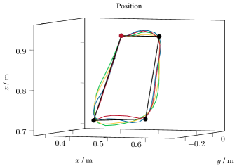
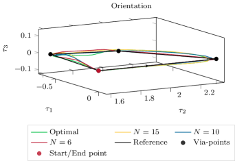
Figure 8: Comparison of the position and orientation trajectories of the MPC solutions for different horizon lengths $N$.

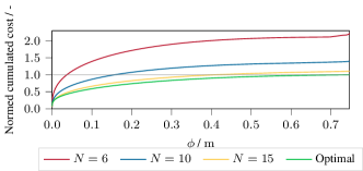
Figure 9: Cumulated cost of the trajectories for different horizon lengths $N$. The curves are normed by the cumulated cost value of optimal solution at $\phi=\phi_{\mathrm{f}}$. Each curve is the cumulated sum of the objective eq. 46 along the resulting trajectories.

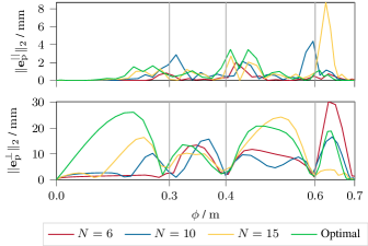
Figure 10: Norm of the tangential and orthogonal position error of the MPC solutions for different horizon lengths $N$.

The influence of the weight $w_{\xi}$ on the path progress is depicted in fig. 11. The figure shows that a larger weight reduces the trajectory duration, see also table 4, since the cost function favors the trajectory progress more strongly.

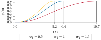
Figure 11: Influence of the weight $w_{\xi}$ on the path progress $\phi(t)$.

The parameters $s_{0}$ and $s_{\mathrm{f}}$ are used in the error bounds in eq. 48 to specify the slopes of the bounding functions at the via-points; see the comparison of the orthogonal errors in fig. 12. The dashed lines indicate the error bounds, which differ only by their slope parameters at the via-points. The parameters influence the error bounds' shape but do not change the maximum value $\Upsilon_{\mathrm{max}}$. A low slope intuitively means that the error bounds around the via-points change slowly; hence, the via-points become more like a via-corridor. A high slope means that this via-corridor becomes very narrow. This is important when discretizing the optimization problem eq. 44, as seen in fig. 12 at the via-points. It shows that the trajectories with a high slope less accurately pass the via-points since the via-corridor becomes too small. The influence of the slope $s_{0}$ and $s_{\mathrm{f}}$ on the trajectory duration, presented in table 4, can be neglected.

Figure 12: Comparison of the orthogonal error trajectories of the position and orientation for different slopes $s_{0}=s_{f}$. The bounds are shown as dashed lines of the corresponding color. Via-points are indicated by vertical gray lines.

10 Experiments

The proposed path planning framework BoundMPC features several important properties, such as position and orientation path error bounding, adhering to via-points, and online replanning, which are required in many applications. Two scenarios will be considered in the following to demonstrate the capabilities of the proposed framework:

1. Moving a large object between obstacles: A large object is moved from a start to a goal pose with obstacles. These obstacles constitute constraints on the position and orientation. Position and orientation paths are synchronized using via-points.

2. Object grasp from a table: An object is grasped using one via-point at the pre-grasp pose. The path must be replanned during the robot's motion in real-time to grasp a different object. Collisions of the end effector are avoided employing asymmetric error bounds.

The Kuka 7-DoF LBR iiwa 14 R820 robot is used for the experiments. The weights for the cost function eq. 46 used in all experiments are listed in table 2, with the weighting matrix $\mathbf{W}_{\xi}$ as the default value $w_{\xi}\phi_{\mathrm{f}}=1$ in table 1. Choosing the planning frequency $f_{\mathrm{c}}=$10\text{\,}\mathrm{Hz}$$ and the number of planning grid points to be $N=10$ leads to a time horizon of $T_{\mathrm{c}}=N/f_{\mathrm{c}}=$1\text{\,}\mathrm{s}$$. The controller considers the next $n=4$ segments of the reference path.

10.1 Moving a large object between obstacles

10.1.1 Goal

This task aims is to move a large object from a start to a goal pose through a confined space defined by obstacles.

10.1.2 Setup

The object is positioned on a table, from which it is taken and then transferred to the goal pose. The obstacles create a narrow bottleneck in the middle of the path. Since the object is too large to pass the obstacles in the initial orientation, the robot must turn it by $90\text{\,}\mathrm{\SIUnitSymbolDegree}$ in the first segment, then pass the obstacles, and finally turn the object back to the initial orientation. BoundMPC allows setting via-points to traverse the bottleneck without collision easily. The path parameter $\phi(t)$ synchronizes the end effector's position and orientation. Thus, the position and orientation via-points are reached at the same time, making it possible to traverse the path safely within the given bounds.

10.1.3 Results

To visualize the robot's motion in the scenario, fig. 13 illustrates the robot configuration in four time instances of the trajectory. For further understanding regarding the basis vectors, fig. 14 displays the position basis vectors $\mathbf{b}_{\mathrm{p,1}}$ and $\mathbf{b}_{\mathrm{p,2}}$ for each linear path segment. The planned trajectory is shown in fig. 15 with the projected error bounds on the Cartesian planes. Five via-points and four line segments are used to construct the reference path. In the second segment, the robot moves with the large object between the obstacles. At the end of the trajectory, the end effector with the large object reaches the desired goal position. Only four via-points are shown in the orientation plot in fig. 15 because the last two via-points coincide. All via-points are passed for the position and orientation. Further details are given in the error trajectories in fig. 16. The low bound in the direction of the basis vector $\mathbf{b}_{\mathrm{p,1,2}}^{\mathrm{T}}=[0,0,1]$ for $e^{\bot}_{\mathrm{p,proj,1}}$ also depicted in fig. 14 by the red arrow in the second segment ensures low deviations in $z$-direction. This bounding does not affect the other error direction $\mathbf{b}^{\mathrm{T}}_{\mathrm{p,2,2}}=[-0.83,0.55,0]$ for $e^{\bot}_{\mathrm{p,proj,2}}$ in this segment, as seen in fig. 16. Furthermore, the last segment for the position is bounded to have low errors for both directions $\mathbf{b}_{\mathrm{p,1,4}}$ and $\mathbf{b}_{\mathrm{p,2,4}}$ with the orthogonal errors $e^{\bot}_{\mathrm{p,proj,1}}$ and $e^{\bot}_{\mathrm{p,proj,2}}$, to ensure a straight motion towards the final pose. The orientation errors $e^{\bot}_{\mathrm{o,proj,2}}$ and $e^{\bot}_{\mathrm{o,proj,2}}$ in the second segment are constrained to be small since only the rotation around the normed reference path angular velocity $\bm{\omega}_{\mathrm{r},2}^{\mathrm{T}}/\lVert\bm{\omega}_{\mathrm{r},2}\rVert_{2}=[0,0,1]$ is allowed to ensure a collision-free trajectory.

Figure 17 compares the actual tangential and orthogonal orientation path errors and their approximations. The true tangential and orthogonal orientation path errors are obtained by eq. 33. The differences are minor, even for large orientation path errors, due to the iterative procedure eq. 58. This shows the validity of the linear approximation for the orientation. A video of the experiment can be found at https://www.acin.tuwien.ac.at/42d0/.

(a) $\phi=$0\text{\,}\mathrm{m}$$

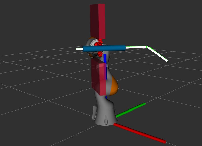
(b) $\phi=$0.6\text{\,}\mathrm{m}$$

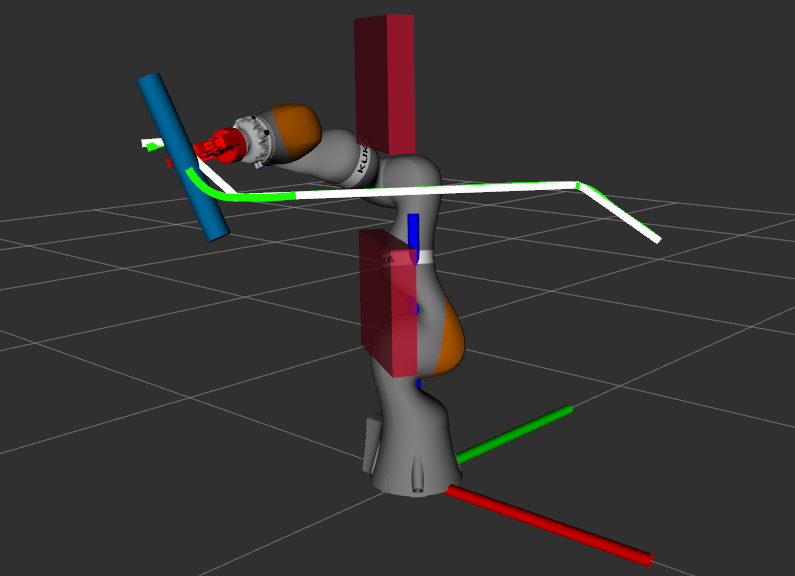
(c) $\phi=$1.1\text{\,}\mathrm{m}$$

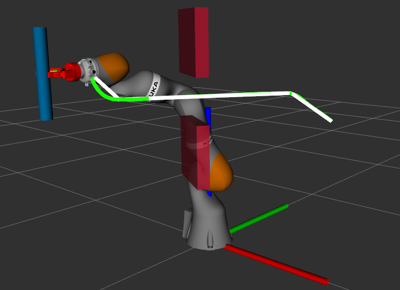
(d) $\phi=\phi_{\mathrm{f}}=$1.37\text{\,}\mathrm{m}$$

Figure 13: Visualization of the robot configurations in different time instances along the path. The red end effector is a gripper attached to the robot flange. The blue cylinder represents the object to be transferred. The red walls are obstacles to be avoided. The white and yellow lines represent the planned trajectory and the reference path of the end effector, respectively. The world coordinate system is given by the RGB (xyz) axes at the base of the robot.

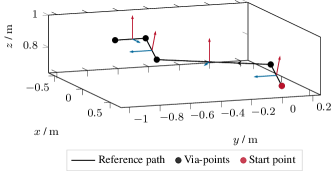
Figure 14: Position basis vectors for each linear reference path segment for the object transfer scenario. The red and blue arrows indicate the basis vectors $\mathbf{b}_{\mathrm{p,1}}$ and $\mathbf{b}_{\mathrm{p,2}}$, respectively, which span the orthogonal position error plane.

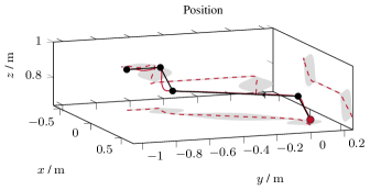
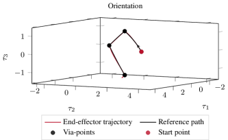
Figure 15: End-effector position and orientation trajectories for the object transfer scenario. The projected bounds (dashed gray areas) for the orthogonal position path error are shown on the Cartesian planes.

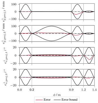
Figure 16: Orthogonal path error trajectories in the position and orientation for the object transfer. The upper two plots show the decomposed orthogonal position path error and the lower two plots the respective orientation path error. The via-points are indicated by vertical gray lines.

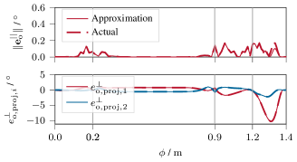
Figure 17: Comparison of approximated and actual orientation path errors in the tangential and orthogonal direction. The via-points are indicated by vertical gray lines.

10.2 Object grasp from a table

10.2.1 Goal

This experiment aims for the robot to grasp an object from a table. The path is replanned during the robot's motion before reaching the object to demonstrate the strength of the proposed MPC framework.

10.2.2 Setup

The grasping pose is assumed to be known. The robot's end effector must not collide with the table during grasping. These requirements can be easily incorporated into the path planning by appropriately setting the upper and lower bounds for the orthogonal position path error. Note that collision avoidance is only considered for the end effector. The replanning of the reference path allows a sudden change in the object's position or a decision to grasp a different object during motion. The newly planned trajectory adapts the position and orientation of the end effector to ensure a successful grasp and avoid collision with another obstacle placed on the table.

10.2.3 Results

To visualize the robot's motion in the scenario, fig. 18 illustrates the robot configuration in six time instances of the trajectory. The trajectories follow the reference path and deviate from it according to the bounds between the via-points. The replanning takes place at $t_{\mathrm{r}}=$5.5\text{\,}\mathrm{s}$$. At the replanning time instance $t_{\mathrm{r}}$, the optimization has to adapt the previous solution heavily due to the change of the reference path. Note that the reference path for the position and orientation in all dimensions changes significantly making this a challenging problem.

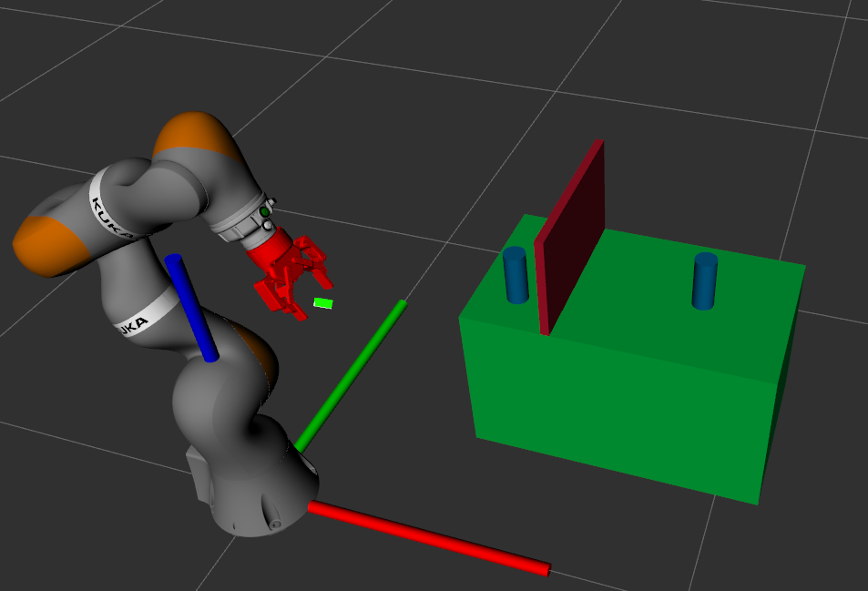
(a) $\phi=$0\text{\,}\mathrm{m}$$

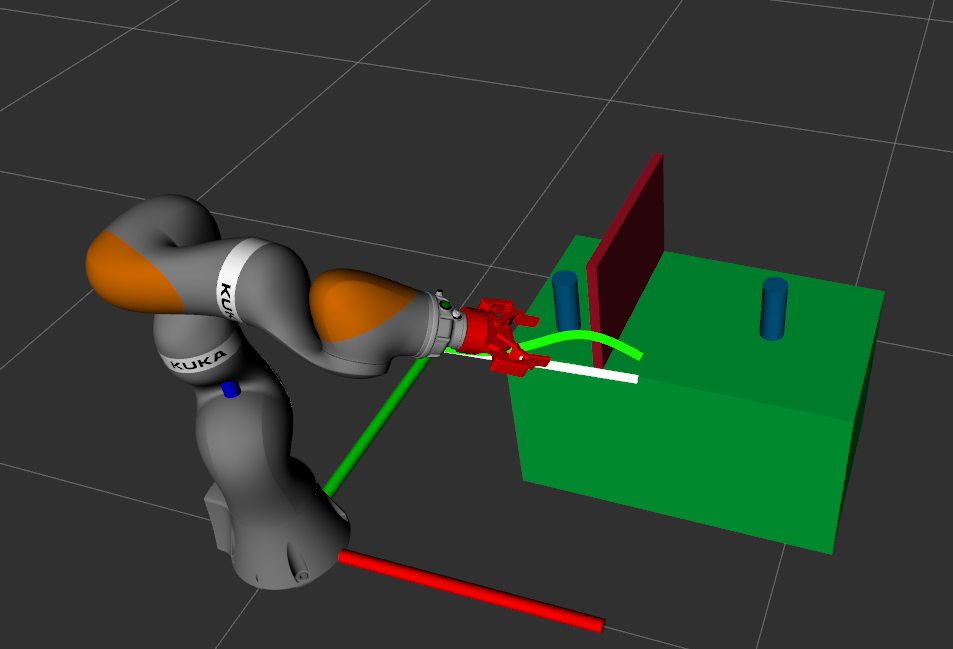
(b) $\phi=$0.3\text{\,}\mathrm{m}$$

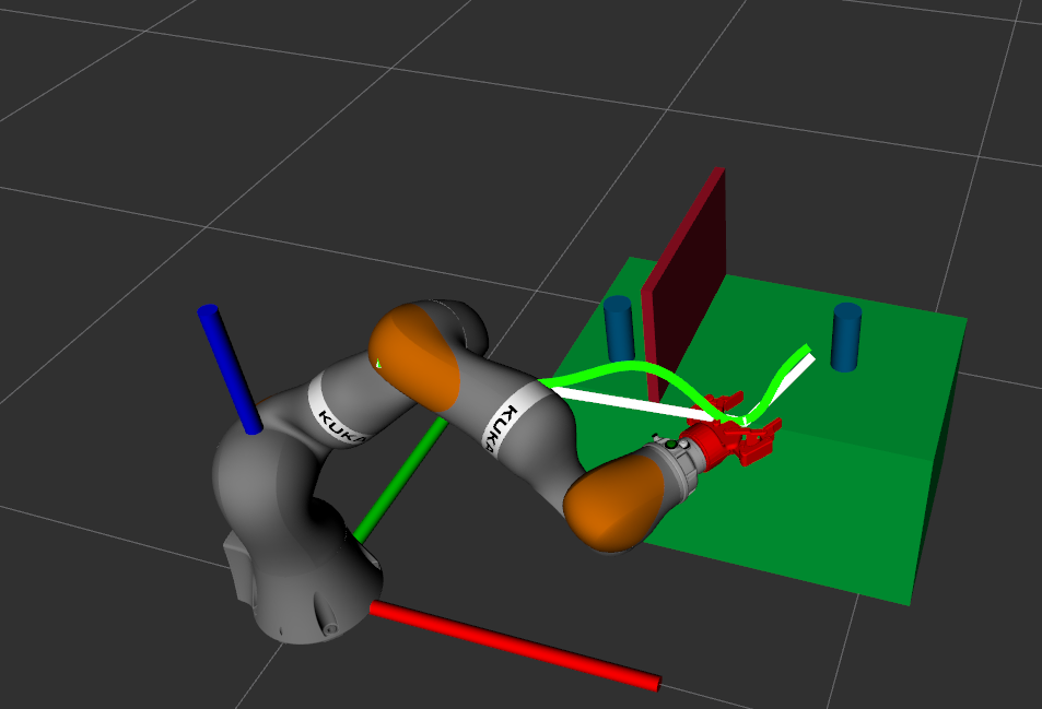
(c) $\phi=$0.6\text{\,}\mathrm{m}$$

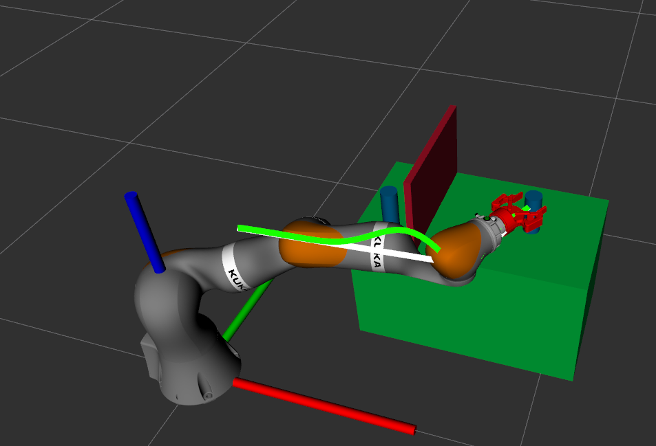
(d) $\phi=\phi_{\mathrm{f,0}}=$0.89\text{\,}\mathrm{m}$$

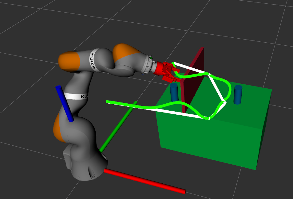
(e) $\phi=$1.1\text{\,}\mathrm{m}$$

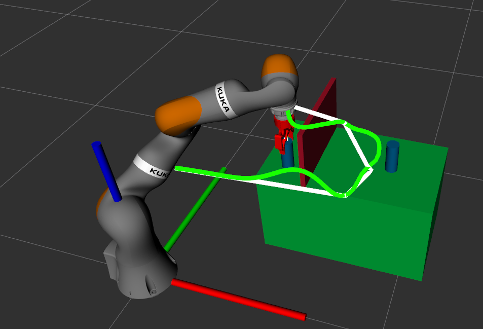
(f) $\phi=\phi_{\mathrm{f,r}}=$1.41\text{\,}\mathrm{m}$$

Figure 18: Visualization of the robot's configuration at different time instances along the path. The red end effector is a gripper attached to the last robot link. The blue cylinders represent the objects to grasp, which are resting on the green table. The red wall is an obstacle to be avoided. The initial reference path has arc length $\phi_{\mathrm{f,0}}$ and is extended to $\phi_{\mathrm{f,r}}$ after replanning. The white and yellow lines show the planned trajectory and the reference path of the end effector, respectively. The world coordinate system is given by the RGB (xyz) axes at the base of the robot.

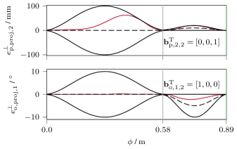
Figure 19: Orthogonal path error trajectories in position and orientation for the object transfer. The upper plot show the orthogonal position path error in basis direction $\mathbf{b}_{\mathrm{p,2}}$ and the lower plot the orthogonal orientation path error in basis direction $\mathbf{b}_{\mathrm{o,1}}$. The via-points are indicated by vertical gray lines.

Figure 20: Orthogonal path error trajectory in in basis direction $\mathbf{b}_{\mathrm{p,2}}$ for the object transfer with replanning. The via-points are indicated by vertical gray lines. At $\phi_{\mathrm{r}}=0.74$, the replanning takes place, indicated by the vertical green line.

The error bounds $e_{\mathrm{p,u},m}$, $e_{\mathrm{p,l},m}$, and $e_{\mathrm{o,u},m}$, $e_{\mathrm{o,l},m}$, $m=1,2$, are chosen asymmetrically such that the error in the $z$-direction is constrained to positive values when approaching the object and the orientation around the $x$-axis is constrained to positive values. This is visualized in fig. 19 for the case of no replanning. Here, the projected position and orientation path errors $e^{\bot}_{\mathrm{p,proj},2}$ and $e^{\bot}_{\mathrm{o,proj},1}$ are bounded by 0 from below or above for the second segment along the basis directions $\mathbf{b}_{\mathrm{p,2,2}}$ and $\mathbf{b}_{\mathrm{o,1,2}}$, respectively. Additionally, the position path error in the basis direction $\mathbf{b}_{\mathrm{p,1}}$ is bounded to be low in the second segment such that the object is approached correctly and to ensure a successful grasp. The basis direction $\mathbf{b}_{\mathrm{p,2,2}}^{\mathrm{T}}=[0,0,1]$ is aligned with the $z$-axis in the second segment to simplify the definition of the bounds. The orientation basis vector $\mathbf{b}_{\mathrm{o,1,2}}^{\mathrm{T}}=[1,0,0]$ represents the orientation around the $x$-axis of the world coordinate system. The upper bounding of the orientation in the second segment ensures that the wrist of the robot does not collide with the table. It can be clearly seen in fig. 19 that all orientation bounds are respected despite the linearization in eq. 42.

Furthermore, fig. 20 shows the orthogonal position path error in the basis direction $\mathbf{b}_{\mathrm{p,2}}$ for the replanned path. Note that for $\phi\leq 0.7$, the trajectory is identical to the one shown in fig. 19. At $\phi_{\mathrm{r}}=0.74$, the replanned trajectory starts and, as discussed in section 7, the error bounds $\Upsilon_{\mathrm{p}}(0.74)=\tilde{\Upsilon}_{\mathrm{p}}(0.74)$ match. For the replanned path, the collision of the end effector with the red object in fig. 18 is avoided by bounding the orthogonal path errors similar to the table. This is not further detailed here. A video of the experiment can be found at https://www.acin.tuwien.ac.at/42d0/.

11 Conclusion

This work proposes a novel model-predictive trajectory planning for robots in Cartesian space, called BoundMPC, which systematically considers via-points, tangential and orthogonal error decomposition, and asymmetric error bounds. The joint jerk input is optimized to follow a reference path in Cartesian space. The motion of the robot's end effector is decomposed into a tangetial motion, the path progress, and an orthogonal motion, which is further decomposed geometrically into two basic directions. A novel way of projecting orientations allows a meaningful decomposition of the orientation error using the Lie theory for rotations. Additionally, the particular case of piecewise linear reference paths in orientation and position is derived, simplifying the optimization problem's online calculations. Online replanning is crucial to adapt the considered path to dynamic environmental changes and new goals during the robot's motion.

Simulations and experiments were carried out on a 7-DoF Kuka LBR iiwa 14 R820 manipulator, where the flexibility of the new framework is demonstrated in two distinct scenarios.

First, the transfer of a large object through a slit, where lifting of the object is required, is solved by utilizing via-points and specific bounds on the orthogonal error in the position and orientation reference paths, which are synchronized by the path parameter. Second, an object has to be grasped from a table, the commanded grasping point changes during the robot's motion, and collision with other objects must be avoided. This case shows the advantages of systematically considering asymmetric Cartesian error bounds.

Due to the advantageous real-time replanning capabilities and the easy asymmetric Cartesian bounding, we plan to use BoundMPC in dynamically changing environments in combination with cognitive decision systems that adapt the pose reference paths online according to situational needs.

Conflict of Interest Statement

The Authors declare that there is no conflict of interest.

References

- [1] Primož Bencak, Darko Hercog and Tone Lerher “Evaluating Robot Bin-Picking Performance Based on Box and Blocks Test” In IFAC-PapersOnLine 55.10, 2022, pp. 502–507 DOI: 10.1016/j.ifacol.2022.09.443
- [2] Valerio Ortenzi et al. “Object Handovers: A Review for Robotics” In IEEE Transactions on Robotics 37.6, 2021, pp. 1–19 DOI: 10.1109/TRO.2021.3075365
- [3] Ting Lei et al. “A Review of Vision-Aided Robotic Welding” In Computers in Industry 123, 2020 DOI: 10.1016/j.compind.2020.103326
- [4] Timm Faulwasser, Benjamin Kern and Rolf Findeisen “Model Predictive Path-Following for Constrained Nonlinear Systems” In Proceedings of the IEEE Conference on Decision and Control, 2009, pp. 8642–8647 DOI: 10.1109/CDC.2009.5399744
- [5] Shen Li, Nadia Figueroa, Ankit Shah and Julie Shah “Provably Safe and Efficient Motion Planning with Uncertain Human Dynamics” In Proceedings of Robotics: Science and Systems, 2021 DOI: 10.15607/rss.2021.xvii.050
- [6] Niels Van Duijkeren et al. “Path-Following NMPC for Serial-Link Robot Manipulators Using a Path-Parametric System Reformulation” In Proceedings of the European Control Conference, 2016, pp. 477–482 DOI: 10.1109/ECC.2016.7810330
- [7] Angel Romero, Sihao Sun, Philipp Foehn and Davide Scaramuzza “Model Predictive Contouring Control for Time-Optimal Quadrotor Flight” In IEEE Transactions on Robotics 38.6, 2022 arXiv:2108.13205 [cs]
- [8] Jon Arrizabalaga and Markus Ryll “Towards Time-Optimal Tunnel-Following for Quadrotors” In Proceedings of the International Conference on Robotics and Automation, 2022, pp. 4044–4050 DOI: 10.1109/ICRA46639.2022.9811764
- [9] Alejandro Astudillo et al. “Varying-Radius Tunnel-Following NMPC for Robot Manipulators Using Sequential Convex Quadratic Programming” In Proceedings of the Modeling, Estimation and Control Conference 55, 2022, pp. 345–352 DOI: 10.1016/j.ifacol.2022.11.208
- [10] Mohamed Elbanhawi and Milan Simic “Sampling-Based Robot Motion Planning: A Review” In IEEE Access 2, 2014, pp. 56–77 DOI: 10.1109/ACCESS.2014.2302442
- [11] Sertac Karaman and Emilio Frazzoli “Sampling-Based Algorithms for Optimal Motion Planning” In The International Journal of Robotics Research 30.7 SAGE Publications Ltd STM, 2011, pp. 846–894 DOI: 10.1177/0278364911406761
- [12] Sven Mikael Persson and Inna Sharf “Sampling-Based A* Algorithm for Robot Path-Planning” In The International Journal of Robotics Research 33.13, 2014, pp. 1683–1708 DOI: 10.1177/0278364914547786
- [13] Thi Thoa Mac, Cosmin Copot, Duc Trung Tran and Robin De Keyser “Heuristic Approaches in Robot Path Planning: A Survey” In Robotics and Autonomous Systems 86, 2016, pp. 13–28 DOI: 10.1016/j.robot.2016.08.001
- [14] Debasmita Mukherjee, Kashish Gupta, Li Hsin Chang and Homayoun Najjaran “A Survey of Robot Learning Strategies for Human-Robot Collaboration in Industrial Settings” In Robotics and Computer-Integrated Manufacturing 73, 2022 DOI: 10.1016/j.rcim.2021.102231
- [15] Takayuki Osa “Motion Planning by Learning the Solution Manifold in Trajectory Optimization” In The International Journal of Robotics Research 41.3 SAGE Publications Ltd STM, 2022, pp. 281–311 DOI: 10.1177/02783649211044405
- [16] Dave Ferguson, Nidhi Kalra and Anthony Stentz “Replanning with RRTs” In Proceedings of the IEEE International Conference on Robotics and Automation, 2006, pp. 1243–1248 DOI: 10.1109/ROBOT.2006.1641879
- [17] Matt Zucker, James Kuffner and Michael Branicky “Multipartite RRTs for Rapid Replanning in Dynamic Environments” In Proceedings of the IEEE International Conference on Robotics and Automation, 2007, pp. 1603–1609 DOI: 10.1109/ROBOT.2007.363553
- [18] Zachary Kingston, Mark Moll and Lydia E Kavraki “Exploring Implicit Spaces for Constrained Sampling-Based Planning” In The International Journal of Robotics Research 38.10-11 SAGE Publications Ltd STM, 2019, pp. 1151–1178 DOI: 10.1177/0278364919868530
- [19] John Schulman et al. “Motion Planning with Sequential Convex Optimization and Convex Collision Checking” In The International Journal of Robotics Research 33.9 SAGE Publications Ltd STM, 2014, pp. 1251–1270 DOI: 10.1177/0278364914528132
- [20] Matt Zucker et al. “CHOMP: Covariant Hamiltonian Optimization for Motion Planning” In The International Journal of Robotics Research 32.9-10, 2013, pp. 1164–1193 DOI: 10.1177/0278364913488805
- [21] Tobias Schoels et al. “CIAO*: MPC-based Safe Motion Planning in Predictable Dynamic Environments” In IFAC-PapersOnLine, 2020, pp. 6555–6562 DOI: 10.1016/j.ifacol.2020.12.072
- [22] Denise Lam, Chris Manzie and Malcolm C. Good “Model Predictive Contouring Control for Biaxial Systems” In IEEE Trans. Contr. Syst. Technol. 21.2, 2013, pp. 552–559 DOI: 10.1109/TCST.2012.2186299
- [23] Sara Spedicato and Giuseppe Notarstefano “Minimum-Time Trajectory Generation for Quadrotors in Constrained Environments” In IEEE Transactions on Control Systems Technology 26.4, 2018, pp. 1335–1344 DOI: 10.1109/TCST.2017.2709268
- [24] Martin Böck and Andreas Kugi “Constrained Model Predictive Manifold Stabilization Based on Transverse Normal Forms” In Automatica 74, 2016, pp. 315–326 DOI: 10.1016/j.automatica.2016.07.046
- [25] Frederik Debrouwere, Wannes Van Loock, Goele Pipeleers and Jan Swevers “Optimal Tube Following for Robotic Manipulators” In IFAC Proceedings Volumes 47.3, 2014, pp. 305–310 DOI: 10.3182/20140824-6-ZA-1003.01672
- [26] Christian Hartl-Nesic, Tobias Glück and Andreas Kugi “Surface-Based Path Following Control: Application of Curved Tapes on 3-D Objects” In IEEE Transactions on Robotics 37.2, 2021, pp. 615–626 DOI: 10.1109/TRO.2020.3033721
- [27] Bernhard Bischof, Tobias Glück and Andreas Kugi “Combined Path Following and Compliance Control for Fully Actuated Rigid Body Systems in 3-D Space” In IEEE Transactions on Control Systems Technology 25.5, 2017, pp. 1750–1760 DOI: 10.1109/TCST.2016.2630599
- [28] Alejandro Astudillo et al. “Position and Orientation Tunnel-Following NMPC of Robot Manipulators Based on Symbolic Linearization in Sequential Convex Quadratic Programming” In IEEE Robot. Autom. Lett. 7.2, 2022, pp. 2867–2874 DOI: 10.1109/LRA.2022.3142396
- [29] Nicolas Torres Alberto, Lucas Joseph, Vincent Padois and David Daney “A Linearization Method Based on Lie Algebra for Pose Estimation in a Time Horizon” In Advances in Robot Kinematics, Springer Proceedings in Advanced Robotics Cham: Springer International Publishing, 2022, pp. 47–56 DOI: 10.1007/978-3-031-08140-8˙6
- [30] Joan Solà, Jeremie Deray and Dinesh Atchuthan “A Micro Lie Theory for State Estimation in Robotics” arXiv, 2021 arXiv:1812.01537 [cs]
- [31] Christian Forster, Luca Carlone, Frank Dellaert and Davide Scaramuzza “On-Manifold Preintegration for Real-Time Visual–Inertial Odometry” In IEEE Trans. Robot. 33.1, 2017, pp. 1–21 DOI: 10.1109/TRO.2016.2597321
- [32] Bruno Siciliano, Enzo Sciavicco, Luigi Villani and Guiseppe Oriolo “Robotics: Modeling, Planning, and Control” London: Springer, 2009
- [33] Thomas Hausberger et al. “A Nonlinear MPC Strategy for AC/DC-Converters Tailored to the Implementation on FPGAs” In IFAC-PapersOnLine 52.16, 2019, pp. 376–381
- [34] Christian Ott “Cartesian Impedance Control of Redundant and Flexible-Joint Robots” Berlin, Heidelberg: Springer, 2008
- [35] Marcelo H. Ang and Vassilios D. Tourassis “Singularities of Euler and Roll-Pitch-Yaw Representations” In IEEE Transactions on Aerospace and Electronic Systems 23.3, 1987, pp. 317–324 DOI: 10.1109/TAES.1987.310828
- [36] Andreas Wächter and Lorenz T. Biegler “On the Implementation of an Interior-Point Filter Line-Search Algorithm for Large-Scale Nonlinear Programming” In Math. Program. 106.1, 2006, pp. 25–57 DOI: 10.1007/s10107-004-0559-y
- [37] Joel A.. Andersson et al. “CasADi: A Software Framework for Nonlinear Optimization and Optimal Control” In Math. Prog. Comp. 11.1, 2019, pp. 1–36 DOI: 10.1007/s12532-018-0139-4