Direct numerical simulations of a cylinder cutting a vortex

Abstract

The interaction between a vortex and an impacting body which is oriented normally to it is complex due to the interaction of inviscid and viscous three-dimensional mechanisms. To model this process, we conducted direct numerical simulations of a thin cylinder intersecting a columnar vortex oriented normally to it. We identified the various stages of the interaction, including the separation of the boundary layer and the generation of secondary vorticity that interacts with the primary vortex. By varying the impact parameter and the Reynolds number, we were able to distinguish the two regimes of interaction mentioned in the literature: the weak and strong vortex regimes. We found that low impact parameters, representing strong vortices, led to ejection and interaction of secondary vorticity from the cylinder’s boundary layer, while high impact parameters, representing weak vortices, led to approximately inviscid interaction of the cylinder with the primary vortex through deformations. We did not find a significant effect of the Reynolds number in the overall phenomenology, even if larger Reynolds numbers lead to the formation of increasingly smaller and more intense vortex structures in the parameter range studied. Finally, we analyzed the hydrodynamic force curves on the cylinder, showing that intense forces could be locally generated for some parameter regimes, but that the average force on the cylinder did not deviate substantially from baseline cases where no vortex was present. Our results shed light on the underlying mechanisms of vortex-body interactions and their dependence on various parameters.

I Introduction

Vortices are one of the most characteristic structures present in fluid flows, and they have been referred to as “the sinews and muscles of fluid dynamics” [1]. At high Reynolds numbers, vortices are generally modelled as singular lines or sheets. A wide variety of flows such as aircraft or propeller-tip wakes or bubble rings can then be studied through the composition of singular solutions [1]. Much attention has been given to how vortex tubes, rings or sheets interact with each other or with solid boundaries, including changes in the topology of singular solutions such as those seen in reconnecting vortex rings [2]. However, the purposeful breaking or “cutting” of topological vortex lines with solid objects has seen less work due to experimental and numerical challenges [3, 4, 5]. This flow phenomenology finds significant relevance in a specific context: blade-vortex interaction (BVI), which involves the intricate physical interaction when a rotating blade encounters a nearby vortex tube [6], but is also present in other physical systems such as Type-II superconductors [7, 8].

BVI holds widespread significance in various engineering applications, spanning wind turbines, helicopter rotors, marine propellers, and industrial fans [6], and due to its practical applications has been the workhorse of research in vortex line cutting in fluid dynamics. The majority of research on BVI concentrates on aerodynamic blades intersecting a straight vortex tube. This specific BVI scenario, referred to as perpendicular or normal BVI, occurs when the vortex and blade axes are perpendicular, and the blade cleaves through the vortex tube. Normal BVI is commonly encountered in applications such as helicopter rotors and wind turbines, where rotating blades confront vortices originating from prior blades or generated by their own motion [9, 10, 11, 12, 13]. We note that other orientations of the blade in relation to the vortex are possible, resulting in other types of BVI: grazing BVI, where the blade is perpendicular to the tube, but it moves in the direction of the core, and parallel BVI [14], where the blade is parallel to the tube, and cuts the tube throughout its extent rather than at a single point. These are outside the scope of our study which focuses on swift cutting of the core.

Experiments and simulations have shown that the interaction between a vortex tube and a body such as a blade or a cylinder depends on various parameters, such as body velocity, vortex core radius, vortex swirl velocity, body geometry and size, and turbulence within the body’s boundary layer [15, 16, 17, 18, 19, 20, 21]. In particular, for a body impacting a vortex with no axial flow, three dimensionless parameters are relevant. These parameters are: (1) the impact parameter ($I_{P}=2\pi\sigma_{0}V/\Gamma$), which is the ratio of the body’s free-stream velocity to the maximum vortex swirl velocity, where $\sigma_{0}$ is the radius of the vortex, $V$ the velocity of the body, and $\Gamma$ the vortex’s circulation; (2) the vortex Reynolds number ($Re_{\Gamma}=\Gamma/\nu$), where $\nu$ is the kinematic viscosity; and (3) the body thickness parameter ($T$), which is the ratio of a characteristic length such as the blade’s curvature or the cylinder diameter $D$, to the vortex core radius $\sigma_{0}$ [22, 17].

Depending on both the response of the primary vortex to the body and about the interaction of the vortex with the body’s boundary layer, response regimes can be constructed depending on the value the dimensionless parameters take. The response regimes are commonly referred to as the weak vortex regime, the strong vortex regime, and the bending regime. The weak vortex regime occurs for thin bodies $(T=D/\sigma_{0}\lesssim 1)$ when the vortex is sufficiently weak $(I_{P}>0.2)$. This regime is characterized with very minimal boundary layer separation and ejection until after the body has penetrated the primary vortex [22]. Once the boundary layer has separated, the separated vorticity becomes entrained within the primary vortex and does not wrap around it, instead spreading away from the body and into the vortex core.

The strong vortex regime has been seen to occur when the vortex is sufficiently strong $(I_{P}<0.08)$ and is independent of the thickness parameter [17]. This regime is characterized with a large amount of interaction between the body’s boundary layer and the vortex prior to the body’s leading edge making contact with the vortex. The ejected vorticity from the body’s boundary layer will roll up into a series of vortex loops that will wrap around the primary vortex. The wrapping of the secondary vorticities creates a series of wave motions that will eventually disrupt the primary vortex. This procedure of primary vortex disruption may also occur when the body is several core radii away from the vortex, but only when the value of the impact parameter is relatively low [3].

The bending regime occurs when the vortex is sufficiently weak $(I_{P}>0.2)$ and the body is sufficiently thick $(T>5)$ [23, 22]. Separation of the boundary layer does not occur before the body has travelled through the original position of the vortex. This regime also sees large scale deformation of the primary vortex due to the inviscid interaction with the body. The core radius of the vortex will thin near the region where the body will impact the vortex due to stretching of the flow about the body. Once the vortex has deformed around the body, the body’s boundary layer will separate and generate wave motions within the vortex eventually leading to a disruption of the vortex [3, 17].

While experimental studies of this process exist, experiments are limited in their access to the full velocity and pressure fields. Furthermore, the effect of turbulence in the boundary layer on the interaction process is not well understood, partly due to the challenges in experimentally controlling inlet turbulence. Numerical simulations could in principle allow a detailed study of the development and evolution of the vortex formation and boundary layer detachment, determining the spatial and temporal forces present on the blade, as well as having full control over the turbulence in the system. They also have the advantage of being able to controlling input parameters separately, i.e. varying $Re_{\Gamma}$ separately from the impact parameter, which is not easy in an experiment.

Inviscid filament models are the oldest method used to simulate BVI, due to their straightforwardness and effectiveness [24, 23, 3]. Essentially, filament models assume that vorticity is concentrated within a tiny filament, and use the Biot-Savart line integral to calculate the resulting velocity field. However, when the integral is evaluated on the filament itself, the result is singular and cannot be used to determine the self-induced velocity of the vortex. To overcome this issue, the domain of integration is typically limited to a specific range that varies with the size and vorticity field of the vortex [24]. Another way to study vortex-body interaction is to use Helmholtz’s law [25, 26]. This approach has been extended to account for variations in the vortex core area during wave propagation. However, a no-penetration condition on the body surface must be ensured, which can be achieved using a vortex sheet [3]. Filament models are particularly useful for predicting how the body will penetrate the vortex or how the vortex will react to the motion of the body [23, 27, 3]. These models have also been used to estimate the pressure on the body surface during the interaction with a vortex, but only up to a certain distance from the body [27]. The distance may vary depending on the impact parameter.

While filament models have yielded promising results, they are limited by the inviscid assumption, and cannot be used to analyze boundary layer separation induced by the vortex. Understanding this phenomena is crucial, because when the body’s boundary layer separates, the ejected vorticity from the boundary layer vorticity interacts with the primary vortex to form secondary vortices, which modifies the interaction process and causes different flow phenomenology in the weak and strong vortex regimes. Even if this process is highly three-dimensional, a number of studies which combine in two-dimensions have been conducted which have hinted at the type of complex flow phenomena which arise. Doligalski et al. [28] analyzed a rectilinear vortex above a flat plate and found evidence of separation and ejection of fluid within the boundary layer into the external flow. Luton et al. [29] found that a weaker vortex or secondary vorticity can redistribute the vorticity of the boundary layer, leading to ejection of boundary layer fluid. A number of three-dimensional studies which combine filaments and viscous boundary layers have been conducted to study the detailed separation process and its evolution in the interaction [30, 31]. These show indications of singular behaviour when using vortex filaments, and cannot fully resolve the dynamics [31].

The highest fidelity simulations of normal BVI available in the literature employ three-dimensional direct numerical simulations of a vortex impacting a blade [5, 32]. These studies have detailed the way a vortex cuts through a blade, and the way this cutting generates circulation and a lift force. Ref. [5] was limited in the range of Reynolds numbers they could simulate, as well as the choice of large impact parameters due to the lack of adequate computational power. Ref. [32] simulates larger Reynolds numbers by fixing the blade Reynolds number to be $Re_{b}=1000$, and varying the strength of the vortex. This study focuses on large impact parameters, $I_{P}>0.5$, and does not access the strong vortex regime.

As can be gathered from above, a detailed numerical study of the separation process in the weak vortex regime and the transition from weak to strong vortex regimes is missing. The use of DNS in vortex-body interaction studies has the potential to clarify previously unclear areas such as the viscous interaction of the body with the vortex [32]. Simulations also allow careful control of the Reynolds number and can assess questions of Reynolds number independence unanswered in experiments [17]. In this manuscript, we set to address these knowledge gaps by conducting three-dimensional direct numerical simulations (DNS) of tube cutting using state-of-the-art numerical techniques. We will simulate a simplified problem: a thin wire (cylinder) impacting normally a high-Reynolds number vortex, and we will study the interaction process by varying two parameters: the impact parameter $I_{P}$ and the circulation Reynolds number $Re_{\Gamma}$, to access the different regimes, and to measure the effect of the Reynolds number on the flow, and on the boundary layer vorticity in particular. By simulating a cylinder, we will enhance the generation of wake turbulence, and can assess how our results differ from those simulations which use blades.

We will focus on key phenomena observed during the interaction. These included the separation and ejection of the boundary layer from the body, the extent of bending in the primary vortex, the emergence from and impact of secondary vortices on the primary vortex, and the topology of major flow structures affecting the induced force on the cylinder, including possible reconnection phenomena. To analyze the flow field, we will employ vorticity visualizations, and calculate the induced force on the cylinder as it cuts through the vortex. We will identify the major flow structures influencing the force curve, and establish qualitative relationships between changes in the impact parameter and circulation Reynolds number.

II Numerical methods

To study BVI, we directly simulate the the incompressible Navier-Stokes equations:

$$\frac{\partial\textbf{u}}{\partial t}+\textbf{u}\cdot\nabla\textbf{u}=-\rho^{-1}\nabla p+\nu\nabla^{2}\textbf{u}+\textbf{f}$$ (1)

$$\nabla\cdot\textbf{u}=0$$ (2)

where u is the velocity, $t$ is time, $\rho$ is the fluid density, $\nu$ is the fluid kinematic viscosity and f is a body force originating from the the immersed boundary method (IBM) forcing used to model the cylinder. A schematic of the system is presented in Figure 1, which shows a cylinder of diameter $D$, with an axis parallel to the $z$-axis travels in the $x$ direction at a velocity $V$ towards a vortex of core-size $\sigma_{0}$ which has an axis parallel to the $y$ direction. This vortex is initialized at the initial time with a Lamb-Ossen (Gaussian) velocity profile with circulation $\Gamma$. We use the vortex circulation $\Gamma$ and the vortex radius $\sigma_{0}$ to non-dimensionalize the system.

Figure 1: Schematic view of the computational domain. The $z$ direction is shortened for clarity.

The computational domain is taken as triply periodic, with periodic lengths $\mathcal{L}_{x}\times\mathcal{L}_{y}\times\mathcal{L}_{z}=30\sigma_{0}\times 30\sigma_{0}\times 90\sigma_{0}$. The larger length in $\mathcal{L}_{z}$ allows for the force on the object to return to baseline values, this effect is fully discussed in Section IV. The simulation is initialized with a zero velocity field except for the Lamb-Ossen vortex with the core extending in the $y$-direction and centered at ($x=0$, $z=0$). The cylinder starts from rest, and travels for $10\sigma_{0}$ at $V$ velocity before reaching the vortex’s core line. Because the distance is the same, this means that for varying cylinder velocity (through changing $I_{P}$), the cylinder reaches the vortex at different times. After cutting the axis of the vortex, the cylinder then travels to the opposing end of the box. This allows us to capture all stages of the interaction with the vortex.

We fix the diameter of the cylinder as $0.95\sigma_{0}$, keeping the thickness parameter $T=D/\sigma_{0}\approx 1$ in the thin regime. We vary the impact parameter between $I_{P}\in(0.05,0.25)$. With our value of $T$, the degree of (inviscid) vortex bending that occurs before the ejection of boundary layer vorticity is determined by the impact parameter. The range of values of $I_{P}$ chosen, which allows us to explore the weak- and strong interaction regimes for low and high values of $I_{P}$ respectively. Finally, we also vary the circulation-based Reynolds numbers in the range $Re_{\Gamma}\in(1000,3000)$ to study the effect of boundary layer turbulence on the system dynamics. The associated cylinder Reynolds number $Re_{c}=VD/\nu$ is calculated as $Re_{c}=\Gamma I_{P}T/(2\pi\nu)=Re_{\Gamma}I_{P}T/(2\pi)$, and varies in the range $Re_{c}\in(7.96,119)$. Table 1 summarizes the control parameters used for all the runs in this manuscript. We note that while the values of $Re_{c}$ used here appear substantially lower than those used in Ref. [32], the reference uses a chord-based Reynolds number, while we use something analogous to a “thickness”-based Reynolds number leading to an order of magnitude discrepancy when comparing $Re_{c}$ to the blade Reynolds number in Ref. [32].

$T$	$I_{P}$	$Re_{\Gamma}$	$Re_{c}$
0.95	0.05	1000	7.56
0.95	0.15	1000	22.7
0.95	0.25	1000	37.8
0.95	0.05	2000	15.1
0.95	0.25	2000	75.6
0.95	0.05	3000	22.7
0.95	0.25	3000	113

Table 1: Control parameters for the simulations of tube-wire interaction in this manuscript.

Simulations are ran using the open-source code AFiD [33]. This code uses energy-conserving second order centered finite differences to spatially discretize the domain. Time marching is done through a third-order Runge-Kutta for the non-linear terms and a second order Crank-Nicolson for the viscous terms. The spatial resolution is taken as $624\times 624\times 1872$, meaning the grid is equally spaced in all directions, with a grid length $\sim 0.05\sigma_{0}\approx 0.05D$. Resolution adequacy is checked by monitoring numerical dissipation. The cylinder is incorporated through the immersed boundary method (IBM) using a moving-least-squares formulation [34]. The surface is discretized using $388800$ triangles. The triangle skewness is $<0.3$, and the average edge length is about $70\%$ of the grid spacing. This ensures adequate resolution without consuming excessive computational resources [34].

III Flow Dynamics for Tube-Wire interaction

III.1 The weak and strong vortex regimes

We initially examine cases at $Re_{\Gamma}=1000$, varying $I_{P}$ to illustrate the difference between the strong and weak vortex regimes. Our analysis begins with visualizing $Q=\partial_{i}u_{j}\partial_{j}u_{i}$ [35], which enables us to focus on the primary vortex. A subsequent discussion of vorticity magnitude will emphasize the wire’s boundary layer and secondary vortices.

Figure 2 depicts a volume rendering of $Q$ for a simulation within the strong vortex regime ($Re_{\Gamma}=1000$, $I_{P}=0.05$). As discussed in Ref. [17] and others, the vortex “pre-senses” the wire’s presence prior to its approach to the core. Even before the wire penetrates the core, the central area of the vortex is disrupted. As the wire gradually traverses the core, numerous secondary structures coil around the primary tube— a detailed analysis of these occurs later during vorticity visualization. By the end of the interaction, little remains of the tube the wire passed through. The BVI process has significantly diminished the vortex’s strength by its conclusion.

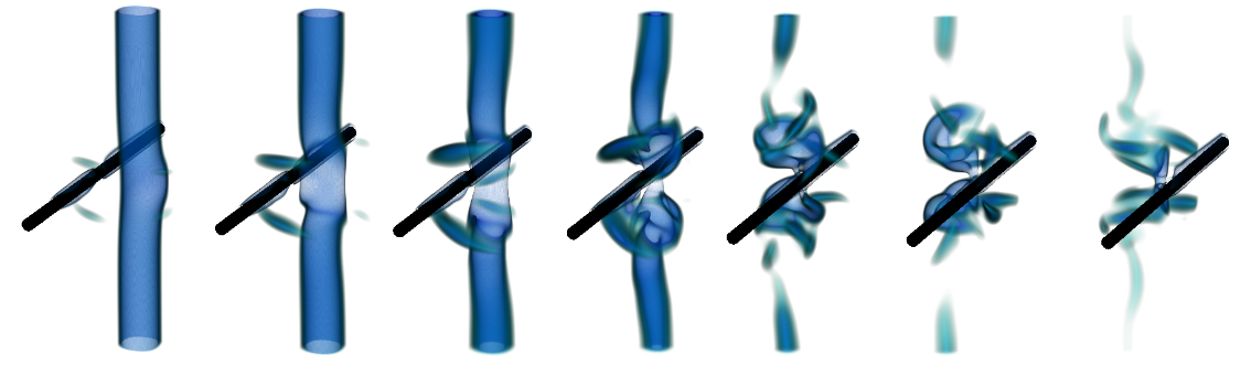
Figure 2: Visualization of the time evolution of $Q$ for a simulation in the strong vortex regime with $Re_{\Gamma}=1000$, $I_{P}=0.05$. Regions in blue indicate regions of strongly negative $Q$. Snapshots are separated $t\Gamma/D^{2}=200$ time-units.

Figure 3 depicts a similar volume rendering of $Q$ in the weak vortex regime ($Re_{\Gamma}=1000$, $I_{P}=0.25$). In this regime, the primary vortex does not “pre-sense” the wire, instead interacting with it solely when it is in close proximity to the vortex core. The vortex swiftly traverses the tube, causing significant deformation to the core. This deformation generates upwards and downwards-propagating waves. As time progresses, the wire completes its passage through the primary vortex tube, leaving behind a minor wake and a distorted tube. Surprisingly, despite the distortion, the “weak” vortex tube displays better resilience compared to the scenario involving a strong vortex. By the end of the BVI process, the waves have transversed the tube and a distorted vortex tube remains behind.

This means that unintuitively, at $Re_{\Gamma}=1000$, a vortex tube endures the “cut” of its core more effectively when encountering a weaker cutting object. This observation warrants further analysis, which we delve into shortly. Primarily, this outcome emerges because the interaction with a slower wire is prolonged, allowing the vortex more time to engage with secondary vorticity originating from the wire. Consequently, this extended interaction disrupts the primary vortex to a greater extent.

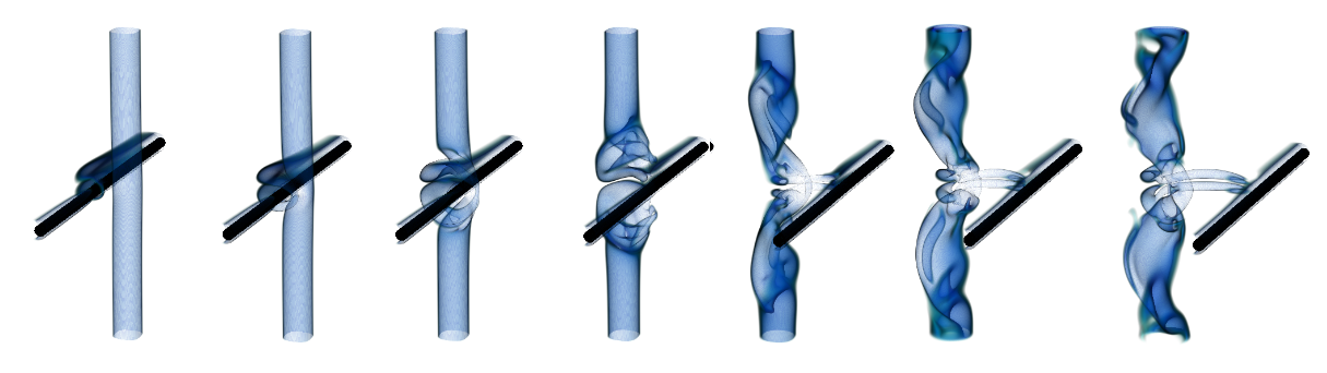
Figure 3: Visualization of the time evolution of $Q$ for a simulation in the weak vortex regime with $Re_{\Gamma}=1000$, $I_{P}=0.25$. Regions in blue indicate regions of strongly negative $Q$. Snapshots are separated $t\Gamma/D^{2}=40$ time-units.

Figure 4 highlights this result by showing $Q$ visualizations for the four simulated cases at various $I_{P}$ values after the wire’s passage. In the case of the smallest $I_{P}$, the vortex experiences complete disruption. However, for $I_{P}=0.15$ and $0.25$, the vortex undergoes deformation, exhibiting propagating waves along its axis, yet retains some coherence. The $I_{P}=0.1$ scenario lies between these extremes, displaying weakening in certain regions and deformation in others. Notably, the extent and nature of disruption in the primary core serve as markers distinguishing between weak and strong vortex regimes. The behavior observed in Figure 4 suggests a smooth transition between these regimes taking place around $I_{P}\approx 0.1$. This was observed in experiments, and a value of $I_{P}\approx 0.08$ was given for the transition between regimes in Ref. [17].

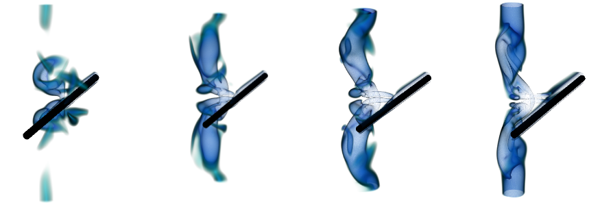
Figure 4: Visualization of $Q$ after the wire has passed through the cylinder axis for $Re_{\Gamma}=1000$, and $I_{P}=0.05$, $0.1$, $0.15$ and $0.25$ (left to right). Regions in blue indicate regions of strongly negative $Q$.

To investigate the role of secondary vorticity in the vortex-wire interaction, our focus turns to vorticity visualization. Beginning with the analysis of the strong vortex regime at $I_{P}=0.05$, Figure 5 presents volumetric representations of the vorticity magnitude $|\omega|$ at $Re_{\Gamma}=1000$. These visuals align with the experimental images and descriptions in Ref. [17]: as the vortex approaches the tube, vorticity from its boundary layer detaches, and begins to curl around the primary tube. Even before the wire approaches the vortex core, this detached vorticity loops once around the main vortex, substantially distorting the core. A compression or stretching of the core occurs around the impact zone due to both the wire and the secondary vorticity, forming a neck region with heightened vorticity magnitude to conserve circulation. Subsequently, the detached vorticity propagates further along the vortex axis, nearly reaching the computational domain’s periodic boundaries. Upon completion of the wire’s cut through the vortex, the primary vortex remains significantly disrupted by the detached secondary vorticity, leaving behind a weakened core. A turbulent cloud of small scale vortices can also be observed when visualizing $|\omega|$. These are rapidly dissipated by viscosity.

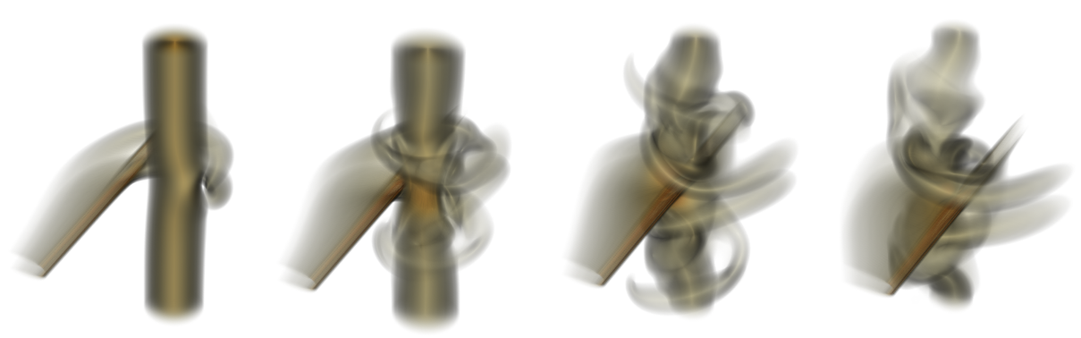
Figure 5: Visualization of the time evolution of $|\omega|$ for a simulation in the strong vortex regime with $Re_{\Gamma}=1000$, $I_{P}=0.05$. Snapshots are at $t\Gamma/D^{2}=740$, $1140$, $1540$ and $1740$.

While these observed flow phenomena mirror those documented experimentally in Ref. [17], our findings expand upon the experimental groundwork in several crucial ways. Firstly, our simulations portray vorticity three-dimensionally rather than photographs of dye visualization. This representation enables us to illustrate the propagation of secondary vorticity through the axis, a phenomenon which is not clear in the experiments, as well as showing the new vortex filaments produced. Secondly, we demonstrate that secondary vorticity arises without the need to introduce turbulence sources either through background flow or vibrations of the structure. Even starting from simple initial conditions, such as a Lamb-Oseen vortex, the secondary vorticity originating solely from the wire’s boundary layer is enough to faithfully reproduce the significant disruptions in the primary vortex seen experimentally. Lastly, we note that our results are symmetrical around the cutting plane in our results due to the absence of axial flow. This shows that the presence of a weak axial flow does not change the phenomenology of strong vortex BVI very much.

In Figure 8, we provide further qualitative data with the vorticity magnitude plotted at the central $x$-$z$ plane for four time instants: before, during, and after core cutting. The first and second snapshots reveal significant detachment and wrapping of vorticity from the wire’s boundary layer before the wire reaches the core, leading to core deformation and vorticity profile redistribution. The third panel, just before impact, displays vorticity amplification due to tube stretching, coinciding with the interaction following a substantial core displacement from its original position. Finally, the fourth panel depicts the remnants of the vortex, significantly weakened and displaced six to seven vortex radii from its initial position. The final core circulation has been reduced to a quarter of its original strength.

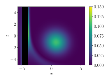
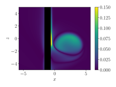
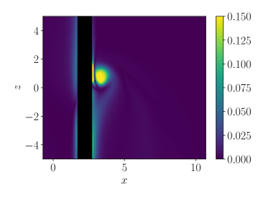
Figure 6: Visualization of the time evolution of $|\omega|$ for a simulation in the weak vortex regime with $Re_{\Gamma}=1000$, $I_{P}=0.05$. Snapshots are at $t\Gamma/D^{2}=540$, $940$, $1340$ and $2340$.

Turning to the weak vortex regime, Figure 7 shows volume plots of the vorticity magnitude $|\omega|$ for $Re_{\Gamma}=1000$ and $I_{P}=0.25$. As in the previous case, two sources of vorticity are evident: the primary vortex and the wire’s boundary layer. However, the overall flow evolution looks very different when compared to Figure 5. The presence of a weaker vortex results in lower induced velocities on the wire. The wire’s boundary layer fails to lift off, so there is no secondary vorticity curling around and deforming the primary vortex before impact. Consequently, the wire’s boundary layer does not play a significant role in this scenario. This lack of interaction before the wire approaches the core serves as a key characteristic of the weak vortex regime, and has facilitated its modeling using inviscid methods.

Instead, in this regime, the core deformation and the propagation of waves dominate, as illustrated in the second and third panels. These deformations arise from the physical presence of the wire traversing the vortex tube, which displaces it and stretches it until the core is eventually “cut”. The point-wise deformation propagates through waves along the primary tube’s axis, previously observed in Figure 3. These do not substantially modify the radius of the primary vortex, a phenomena observed in the simulations and experiments of weak-vortex BVI with axial flow in Ref. [22]. This flow behavior differs from BVI with axial flow in the weak vortex regime. Axial flow introduces a notable asymmetry in wave propagation, an aspect absent in our current observations. Additionally, the object’s presence obstructs the axial flow, creating “compression” and ’expansion’ regions that modify the vortex radius [22].

Finally, the fourth panel depicts the wire after cutting through the tube, leaving a wake that interacts with the strongly deformed vortex tube. Over time, the vortex manages to reconstitute itself and survive the cutting, albeit with a significantly altered vorticity profile, as shown in the last panel. The primary vortex has also entrained a small quantity of vorticity from the boundary layer, as suggested by Ref. [22]. We also note that in this case, we were able to observe some of the phenomena usually attributed to the bending regime, i.e. deformations of the primary vortex, and a stretching of the core near the impact location. This hints at the fact that the transition between strong vortex and bending regimes, which is outside the scope of this paper, will also be smooth.

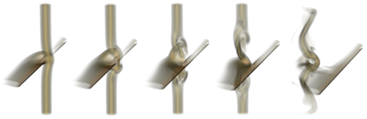
Figure 7: Visualization of the time evolution of $|\omega|$ for a simulation in the weak vortex regime with $Re_{\Gamma}=1000$, $I_{P}=0.25$. Snapshots are at $t\Gamma/D^{2}=200$, $240$, $280$, $320$ and $440$.

These observations are underscored in Figure 8, where the vorticity at the center $x$-$z$ plane is depicted for four distinct time points—prior to, during, and after the core cutting. In the first panel, we show the wire approaching the vortex, which remains as a circular path of vorticity. In the second panel, the vorticity originating from the wire is beginning to wrap around the vortex, but at a slow rate. It is not fast enough to surround the vortex before the main wire reaches the core. Notably, although the vorticity has less time to detach, it exhibits a higher value than in Figure 6. This can be attributed to the non-dimensionalization using $\Gamma/\sigma$ as a velocity scale, where higher values of $I_{P}$ lead to greater wire velocities, resulting in larger vorticity values for a boundary layer when normalized using $\Gamma$-$\sigma$ units.

In the third panel, the vortex has already shifted from its initial position, with intensified vorticity due to stretching. Finally, in the fourth panel, the wire has completely traversed the vortex, leaving behind vorticity associated with the primary tube. The distribution differs, with vorticity concentrated in a thin sheet and displaced to the right by a few vortex cores. Despite this, a comparison of the initial and final circulation of the vortex reveals only a $5\%$ loss throughout the entire process. This showcases the vortex’s ability to withstand the interaction significantly better than the case at $I_{P}=0.05$, which suffered a $75\%$ loss of its original circulation.

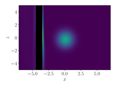
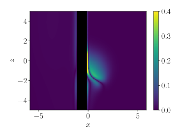
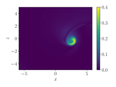
Figure 8: Visualization of the time evolution of $|\omega|$ for a simulation in the weak vortex regime with $Re_{\Gamma}=1000$, $I_{P}=0.25$. Snapshots are at $t\Gamma/D^{2}=120$, $200$, $240$ and $400$.

We can quantify the loss of circulation after the interaction has taken place ($\Gamma_{f}$) for all cases. This is shown in figure 9, where we plot $\Gamma_{f}/\Gamma_{0}$, $\Gamma_{0}$ being the original circulation of the vortex. We observe from the plot that the amount of circulation in the vortex by the end of the interaction monotonically increases with $I_{P}$ in the range studied. We note that this trend cannot persist, as the circulation must saturate at $\Gamma_{f}\approx\Gamma_{0}$ at higher values of $I_{P}$, as it is not expected that the wire imparts additional circulation to the vortex.

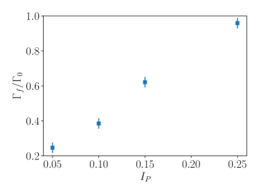
Figure 9: Loss of circulation during the interaction quantified as the ratio between final and initial circulations as a function of $I_{P}$ for the four cases simulated at $Re_{\Gamma}=1000$.

III.2 The effect of Reynolds number

Up to now our discussion has been limited to $Re_{\Gamma}=1000$. Many hydrodynamical instabilities of vortex tubes set in at values of $Re_{\Gamma}$ which are similar or slightly higher [36]. Therefore, expanding our analysis to higher Reynolds numbers will not only assess the Reynolds number’s influence on BVI but could also lead to very different outcomes due to the heightened instability of the resulting vortices.

To explore this, we commence by visualizing the time evolution of vorticity in the strong vortex regime at $Re_{\Gamma}=3000$ and $I_{P}=0.05$ in Figure 10, which offers a comparison with the $Re_{\Gamma}=1000$ counterpart shown in Figure 5. An initial inspection reveals seemingly minor differences between both cases. The lifted secondary vorticity from the boundary layer exhibits higher values but looks thinner, consistent with the increased Reynolds number of the wire. The fundamental flow mechanisms seem largely unaffected: a thinning of the core near the impact point, the formation of a neck-like structure, and an increase of vorticity. Moreover, the secondary vortices lifting off and wrapping around the vortex propagate through its axis at a comparable speed. Key disparities include heightened distortion of the primary vortex, now featuring smaller wavelength components, and that the turbulent cloud left behind is formed from smaller structures. Notably, unlike the $Re_{\Gamma}=1000$ scenario where remnants persisted, at $Re_{\Gamma}=3000$, we cannot identify a similar remnant of the primary vortex after the interaction has taken place, preventing the calculation of a value for $\Gamma_{f}$ as previously done.

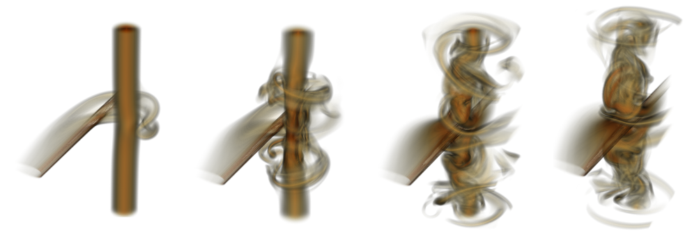
Figure 10: Visualization of the time evolution of $|\omega|$ for a simulation in the strong vortex regime with $Re_{\Gamma}=3000$, $I_{P}=0.05$. Snapshots are at $t\Gamma/D^{2}=740$, $1140$, $1540$ and $1740$.

To better appreciate the effect of the higher Reynolds number, we show the vorticity magnitude in a cut through the $z=0$ plane just before the impact of the cylinder for the two Reynolds numbers simulated. The flow features remain qualitatively similar, even if the right panel shows sharper features: the wrapping of vorticity around the primary tube, as well as its role in forming the neck can be observed. This underscores the importance of secondary vorticity in the strong vortex regime, as postulated in Ref. [17]. Models of normal BVI within the strong vortex regime must adequately incorporate this phenomenon as it plays a pivotal role in driving the dynamics.

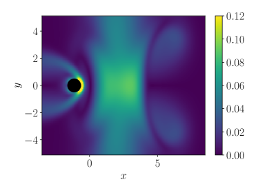
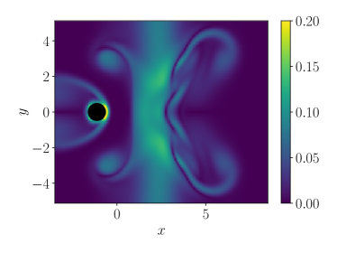
Figure 11: Vorticity magnitude in the $z=0$ plane just before impact ($t\Gamma/D^{2}=940$) for $I_{P}=0.05$ and $Re_{\Gamma}=1000$ (left) and $Re_{\Gamma}=3000$ (right).

Turning to the weak vortex case ($I_{P}=0.25$), we present visualizations of the vorticity modulus in Figure 12, again allowing for a comparison with Figure 5. Similar to observations at lower Reynolds numbers, there is negligible vorticity detachment from the cylinder. The primary tube displays analogous deformation patterns followed by wave propagation, consistent with the findings at lower Reynolds number. At later stages, increased distortion and emergence of smaller scales can be seen which are due to the increased tendency towards instability at this $Re_{\Gamma}$ value. Despite these developments, the tube survives the cut. The remnants left behind be observed in the last panel, at the end of the interaction. However, this tube has only about $85\%$ of the initial circulation left, as a fraction of it will have been lost to the small scale structures which arise and dissipate.

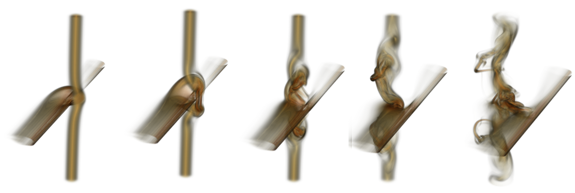
Figure 12: Visualization of the time evolution of $|\omega|$ for a simulation in the strong vortex regime with $Re_{\Gamma}=3000$, $I_{P}=0.25$. Snapshots are at $t\Gamma/D^{2}=200$, $240$, $280$, $320$ and $440$.

Additionally, we also show the vorticity magnitude through the $y=0$ plane just before the cylinder’s impact in the weak vortex regime for the two Reynolds numbers simulated. In this regime, the two cases look practically identical, aside from the higher values of vorticity and the thinner boundary layers. Notably, this shows that flow models which neglect secondary vorticity could adequately capture the interaction within this regime, primarily driven by deformations induced by the moving object.

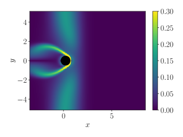
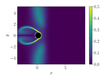
Figure 13: Vorticity magnitude in the $z=0$ plane just before impact ($t\Gamma/D^{2}=220$) for $I_{P}=0.25$ and $Re_{\Gamma}=1000$ (left) and $Re_{\Gamma}=3000$ (right).

From these findings, it becomes evident that the primary control parameter in BVI is the impact parameter $I_{P}$. Varying the Reynolds number results in amplified distortion along the primary vortex, driven either by secondary vorticity or wave propagation. However, these alterations do not significantly impact the fundamental collision features, at least up to $Re_{\Gamma}=3000$. Furthermore, our simulations successfully reproduce and provide reasoning for most experimental outcomes, demonstrating that even in the absence of turbulence, the phenomenology of weak and strong BVI can be faithfully replicated.

IV Forces on the wire

IV.1 Initial Remarks

We now move to an area which is much less analyzed in BVI: measurement of the force on the cylinder. However, an adequate definition of the force on is not simple. Two things have to be taken into account: first, the force coming from BVI is a deviation from a constant drag which resists the movement of the cylinder at a constant velocity in a quiescent flow. Secondly, this deviation will be localized to the point of interaction, and if we add up the forces for a quasi-infinite cylinder or blade undergoing BVI, they would be approximately the same for those where there is no BVI, as the constant drag would overwhelm the forces from BVI.

To elaborate on this, in the left panel of Figure 14 we show the force coefficient distribution $C_{f,x}=f_{x}/(\frac{1}{2}\rho[\Gamma/\sigma]^{2})$ on the cylinder for the weak vortex case ($I_{P}=0.25$, $Re_{\Gamma}=1000$) before the cylinder has reached the vortex core. We note that this representation is highly distorted as the cylinder is very long. However, it is useful to note a few things. First, we can observe that the distribution is symmetric around $\theta=0$, which corresponds to the leading edge of the cylinder. This is a natural product of the symmetry of the system. Second, we note that while the region of strongest interaction is closely localized to the impact point, as could be expected, the return to asymptotic values is rather slow. Finally, we note that a rather small region of the cylinder sees an overall force in the direction of motion of motion of the cylinder ($C_{f,x}>0$). This is due to the fact that locally the flow direction can be reversed when the velocity induced due to the vortex is larger than the cylinder motion.

We emphasize these results on the middle panel of Figure 14, which shows the force on the cylinder along its axis $C_{f}(z)$. The baseline case where no vortex is present is shown as a solid line. The forces can be seen to be somewhat symmetrical around $z=0$, i.e. the collision point. The overall force again shows positive values, coincident with regions where the velocity the cylinder sees is reversed. Finally, a long tail decay is observed: the forces do not return to the baseline case even at the edges of the cylinder. We note that our simulations yield qualitatively similar curves to those presented in the simplified models of Ref. [23], with the presence of a suction peaks and regions of increased pressure. However, comparison is difficult due to the simplifying assumptions made of the flow and the different parameter regimes investigated.

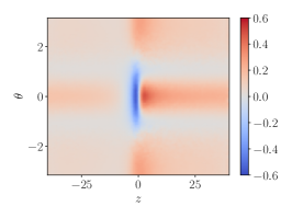
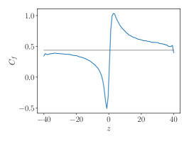
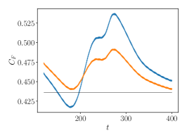
Figure 14: Left: Pressure coefficient along the cylinder for $Re=1000$, $I_{P}=0.25$ at time $t\Gamma/D^{2}=160$. Middle: Force coefficient along the cylinder axis for the same case. Left: Evolution of drag coefficient with time for the full cylinder (orange) and half the cylinder (blue).

As a final step we can calculate the average drag coefficient. If we use the entire extent of the cylinder, we obtain a value of $C_{F}=0.449$. If we integrate the force using the half of the cylinder closest to the vortex, and discard the two quarters close to the edges, we obtain a value of $C_{F}=0.428$. While both values are almost indistinguishable from the baseline value of $C_{F}=0.436$, one deviates upwards and the other downwards. These problems of adequately calculating $C_{F}$ are showcased in the right panel of Figure 14, which shows the time evolution of $C_{F}$ calculated using the full cylinder and half the cylinder. Both values show similar trends of increasing and decreasing during stages of the collision. However, they can be either above or below the baseline value depending on the cylinder segment considered for calculation. In any case, the deviations are mild, and only reach a maximum of $~{}20\%$ drag increase for the half-cylinder calculation. We also note that some small oscillations are present in the force calculation, which have a frequency close to the natural frequency of the cylinder $D/V$.

Due to the problems of adequately defining $C_{F}$, we choose not to represent it for other cases and will only show the evolution of $C_{f}(z)$ for a few select cases below.

IV.2 Results

In this section, we show $C_{f}(z)$ for a few selected time instants for four characteristic cases. These are two cases for each of the strong ($I_{P}=0.05$) and weak ($I_{P}=0.25$) vortex regimes, at the two Reynolds numbers simulated. These are shown in Figure 15.

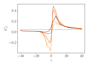
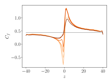
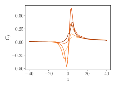
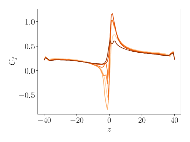
Figure 15: Force coefficient along the cylinder axis at several time instances. Left column is cases at $I_{P}=0.05$, while right column is cases at $I_{P}=0.25$. Top row is at $Re_{\Gamma}=1000$, while bottom row is at $Re_{\Gamma}=3000$. Symbols: left column ($I_{P}=0.05$), light to dark: $t\Gamma/D^{2}=700$, $1100$, $1500$, $1900$ and $2300$. Right column ($I_{P}=0.25$), light to dark: $t\Gamma/D^{2}=160$, $200$, $220$, $240$, $280$ and $320$.

We first start by discussing the case with $I_{P}=0.05$ and $Re_{\Gamma}=1000$. We notice that the curves are relatively similar to those shown in the previous subsection. The curves deviate from the baseline value, and they are roughly antisymmetrical around the collision point $z=0$. The deviations increase as the cylinder approaches the vortex, but they reach a maximum at distinct times: the peak force inversion ($C_{f}>0$) happens earlier than the peak suction ($C_{f}<0$). In the same manner, the values in the force inversion side return to the baseline values earlier than in the suction side. This is probably due to the fact that the cylinder boundary layer is being lifted up earlier from the force inversion side, so the interaction happens first on this half of the cylinder. Finally, we note that the deviations from the baseline value are much more significant in this case: after all, the vortex is strong. This means that it will create forces on the cylinder which are much larger than those originating solely from the ordinary drag force.

Turning to the case with $I_{P}=0.25$ and $Re_{\Gamma}=1000$, we notice that the behaviour of the force has some similarities but also some differences when compared to the earlier case. The main difference is that the forces in the regions of large positive $C_{f}$ fluctuate much less- it attains a maximum value and remains close to that maximum value for most of the interaction. This suggests a probable absence of significant boundary layer liftoff. On the cylinder half experiencing force reversal, temporal variations are more pronounced yet localized due to the weaker vortex. In essence, little more can be extrapolated from these observations.

Finally, we show the Reynolds number dependence of the force in the bottom panels of Figure 15, which can be contrasted to the top row. We note a relatively weak dependence of behavior on Reynolds number. The primary difference lies in the smaller baseline values of $C_{F}$, yet both curves exhibit analogous behaviour. Close to the impact point, spatial oscillations in $C_{f}(z)$ become more discernible, likely owing to the influence of smaller and more intense vortical structures on the cylinder.

In essence, our investigation into the forces on the cylinder reveals that while locally, BVI can generate substantial forces, especially within the strong vortex regime, these forces tend to average out across the cylinder halves facing either positive or negative vortex velocities. Consequently, the average force remains relatively consistent.

V Summary and conclusions

In this manuscript we have conducted direct numerical simulations of normal body-vortex interaction using a thin cylinder. We focused on the transition and the differences in the weak and strong vortex regimes, confirming that it is a smooth transition, primarily driven by the capacity of the cylinder’s boundary layer to detach and wrap around the primary vortex before impact takes place. In the strong vortex regime, this detached, or secondary vorticity propagates along the vortex’s axis, interacting with it and heavily debilitating it, with the result that by the end of the interaction the vortex has almost dissipated. In the weak vortex regime, the cylinder only interacts with the vortex once the body reaches the tube. It then deforms it, propagating waves along the axis, which do not require the modelling of the cylinder’s boundary layer to capture adequately. The behavior of the waves was significantly different to those observed when axial flow is present.

We also investigated the Reynolds number dependence of the flow, showing that while the large contours of behaviour do not change, the vortices left after interaction are much more unstable and show increased turbulence. This also indicates that even in the absence of of background turbulence, the flow left behind the cylinder will become turbulent. These findings both reproduce existing experimental data [22, 17] when the presence of axial flow is not important, and confirm that modelling of the viscous effects are necessary to capture the intricacies of the strong vortex regime. Finally, we measured the force on the cylinder, and showed that while deviations from the baseline values are present, and the force can locally invert direction, the overall force from the interaction is concentrated close to the impact point, and that it averages out on both sides of the interaction.

Our primary interest when simulating normal BVI was on “cutting” vortex lines. However, these simulations showed that the phenomenology is much more complicated, especially for the strong vortex case, and that the interaction deviates from what one could expect from ideal vortex models. While we have examined here normal BVI, with minor modifications the code could be extended to simulating parallel and grazing BVI, and regimes in between. Another possible extension of this work is the question of what happens when a vortex ring- and not a vortex tube is cut. Very few studies of cutting a vortex ring with a wire have been made [4]. Novel structures such as “elephant ears” have been reported, which have not been related to the wider literature on BVI.