Contact-angle hysteresis provides resistance to drainage of liquid-infused surfaces in turbulent flows
Abstract
Lubricated textured surfaces immersed in liquid flows offer tremendous potential for reducing fluid drag, enhancing heat and mass transfer, and preventing fouling. According to current design rules, the lubricant must chemically match the surface to remain robustly trapped within the texture. However, achieving such chemical compatibility poses a significant challenge for large-scale flow systems, as it demands advanced surface treatments or severely limits the range of viable lubricants. In addition, chemically tuned surfaces often degrade over time in harsh environments. Here, we demonstrate that a lubricant-infused surface (LIS) can resist drainage in the presence of external shear flow without requiring chemical compatibility. Surfaces featuring longitudinal grooves can retain up to 50% of partially wetting lubricants in fully developed turbulent flows. The retention relies on contact-angle hysteresis, where triple-phase contact lines are pinned to substrate heterogeneities, creating capillary resistance that prevents lubricant depletion. We develop an analytical model to predict the maximum length of pinned lubricant droplets in microgrooves. This model, validated through a combination of experiments and numerical simulations, can be used to design chemistry-free LISs for applications where the external environment is continuously flowing. Our findings open up new possibilities for using functional surfaces to control transport processes in large systems.
I Introduction
Functional surfaces that have the ability to regulate mass, energy and momentum transport in a fluctuating fluid flow could significantly reduce energy waste in various applications, including marine infrastructure, medical devices, thermal systems and food processing units. One promising technology that has emerged is lubricant-infused surfaces (LISs), which use microstructures to trap a lubricating liquid [1, 2] [1, 2]. The presence of a lubricant offers several ways to interact favourably with external fluid flows. The interface between the lubricant and the overlying liquid is slippery, preventing the attachment of microorganisms and resulting in an efficient anti-fouling surface [3, 4, 5]. Additionally, the flow over a LIS experiences slippage, reducing the frictional resistance exerted on the surface [6, 7, 8, 9, 10]. Moreover, the external flow can set the trapped lubricant into recirculating motion, enhancing heat and mass transfer rates between the surface and the bulk flow [11].
Previous studies on submerged LISs have relied on a chemical compatibility rule that was primarily developed for liquid-repellent and anti-adhesive applications [2, 1, 12, 13]. According to this rule, the chemistry of the surface needs to be similar to the chemistry of the lubricant to avoid dewetting. However, achieving chemical compatibility poses a significant challenge for large-scale applications. Most techniques used to tune solid surface energy involve spray coating or thin film deposition [14, 15, 16], which can be time-consuming and costly when applied to large surface areas. In addition, chemically modified surfaces degrade over time due to exposure to UV light, humidity, chemicals or stresses during handling. An alternative approach of achieving chemical compatibility is selecting a lubricant and a solid with a high affinity. However, such combinations are limited and based on hydrophobic polymers and other inert lubricants that raise environmental concerns as their inertness makes them difficult to degrade naturally [17].
In this study, we characterize the physics of LISs in the presence of an external fluid flow when the chemical compatibility rule is broken. We find that the substrate can retain a significant amount of lubricant by relying on contact-angle hysteresis (CAH). Small-scale physical or chemical inhomogeneities naturally appearing on the substrate pin the lubricant-liquid-solid contact line and create a capillary force that resists lubricant depletion. The size of the pinning force does not depend on the equilibrium contact angle , but instead on the difference between the advancing () and receding () contact angles. This implies that the condition that the lubricant must preferentially wet the surface rather than the overlying liquid is not strictly necessary for a LIS submerged in liquid that flows. We develop a theoretical model that provides an explicit expression for a priori predicting the maximum length of a lubricant droplet given the surface geometry, CAH and external friction force. Our criterion applies in turbulent flow environments, showing that the retention mechanism is robust under unsteady and fluctuating external stresses. Moreover, we use the model to introduce a non-equilibrium design rule for chemistry-free LISs. The rule provides novel opportunities for manufacturing lubricant-infused surfaces to control transport processes in large-scale flow systems.
II Experimental configuration and methods
II.1 Turbulent channel flow facility
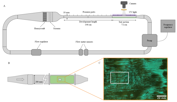
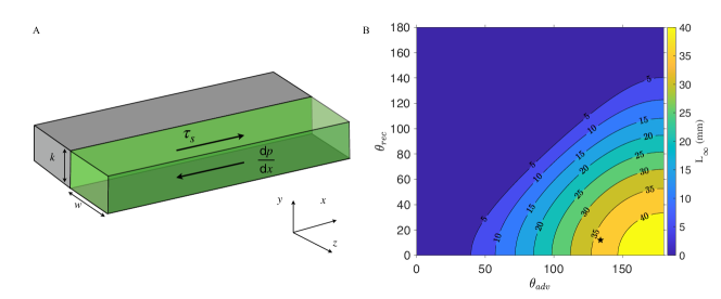
We use a water channel facility to characterize the behavior of liquid-infused surfaces in turbulence. The flow facility, shown schematically in Fig. 1A, has the width and the height , resulting in an aspect-ratio of 20:1. The flow is developed over a length of before reaching the test section which measures in length.
For a fully developed turbulent channel flow, which has a mean velocity that is uniform in the spanwise and streamwise directions, the mean wall shear stress (WSS) , can be obtained from the force balance,
| (1) |
Here, represents the mean pressure gradient, which is obtained by measuring the difference between each pressure port and the most upstream one with a series of piezoelectric miniature transducers (see Fig. 1). Tab. 1 presents the mean WSS obtained from (1) on a smooth solid wall for three different bulk velocities () . The bulk velocities range from m/s to m/s, resulting in mean WSS from Pa to Pa. These values correspond to bulk Reynolds number (with being the fluid viscosity) ranging from 9100 to 15600 and skin friction coefficient (where is the fluid density) from to . To investigate if the facility generates a canonical turbulent channel flow, we compare the obtained from measurements with the empirical relation proposed by Dean [18], given by . Tab. 1 demonstrates a sufficiently good agreement between the skin-friction coefficients for the purposes of our investigation. In a similar way, Tab. 1 compares the measured friction Reynolds number, – ranging from 280 to 442 – with the empirical relation , where again a reasonable agreement is observed. The main sources of error are attributed to the accuracy of the pressure sensors and to temperature variations, which were seen to vary by approximately one degree over five minutes of flow at the highest flow rate.
| Quantity | Acquisition/Expression | Case 1 | Case 2 | Case 3 |
|---|---|---|---|---|
| (m/s) | Ultrasonic flowmeter | 0.91 0.01 | 1.30 0.01 | 1.56 0.02 |
| (Pa) | Pressure transducers | 3.2 0.7 | 5.8 0.8 | 7.8 1.0 |
| 9100 | 13000 | 15600 | ||
| 7.73 | 6.86 | 6.41 | ||
| 7.47 | 6.84 | 6.53 | ||
| 283 | 381 | 442 | ||
| 275 | 376 | 442 |
II.2 Liquid-infused surfaces
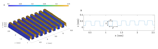
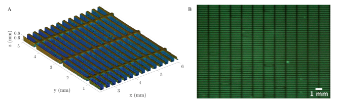
The liquid-infused surface is flush-mounted to the lower wall of the test section. The texture consists of longitudinal (i.e. parallel to the flow direction) grooves fabricated using UV-lithography (described in App. A). Fig. 2 shows a portion of the groove geometry and the corresponding profile. The grooves have depth m, width m and pitch m. Before mounting the panel with the substrate on the channel wall, the grooves are infused with hexadecane (Sigma-Aldrich) (viscosity ratio with respect to water and lubricant-water surface tension ). The surfaces are then slightly tilted for 5 minutes to drain the excess lubricant by gravity. The final sample, composed by four adjacent substrate tiles, covers the full area of the test section wall with an extension of . The upper wall is made of a smooth clear acrylic plate that allows for optical access. To visualise the lubricant-water interface during the flow experiments, a fluorescent imaging technique is used. The lubricant fluid is mixed with a fluorescent dye (Tracer Products TP-4300) at a volume ratio 2:1000. A series of UV LED lights, fixed to the test section, excite the dye which emits a green glow. Fig. 1C shows how the lubricant appears during a flow experiment. Using a digital camera (Nikon D7100 DSLR) with a Nikon AF Micro-Nikkor lens and a yellow filter, consecutive images are taken at a selected time interval. The resolution of the photos is 160 px/mm. The field of view (FOV) of the camera is mm2 and it is located at the centre of the test section, as represented in Fig. 1B. The duration of the measurements is two hours for each experiment.
The surface chemistry together with the substrate geometry determines the spontaneous spreading of the lubricant in the textured surface in the presence of water. For our solid substrate, which has the geometry of a rectangular groove with width and depth , the surface energy per unit length due to a displacement is given by [19],
where are the surface tensions between the different phases: lubricant droplet (), solid substrate (), and the immiscible surrounding liquid (). The lubricant will wick into the groove when it is energetically favourable (), i.e.
By defining spreading parameter as , we can write the condition above,
| (2) |
When the spreading condition (2) is satisfied, a lubricant droplet will spread in the groove until a thin film is formed. In this scenario, for which the lubricant and the solid are chemically compatible, the LIS is called wetting. On the other hand, when (2) is not satisfied, the droplet will only partially wet the grooved surface, and a triple-phase contact line appears. In the latter configuration, the lubricant-solid combination is chemically incompatible and the LIS is partially wetting.
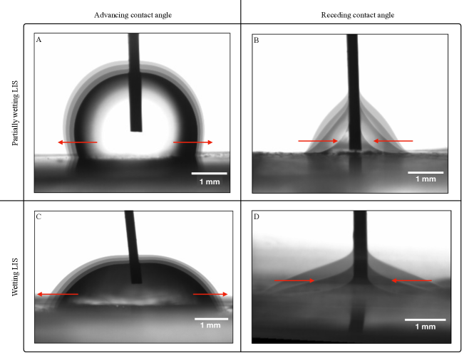
Tab. 2 shows the equilibrium chemical properties of the partially wetting LIS and the wetting LIS that we have used in this study. The former has untreated polymeric substrate (see App. A), whereas the latter surface is functionalised with a hydrophobic coating. We measured the equilibrium contact angle () of a lubricant droplet immersed in water on smooth samples with the sessile drop method [20]. We observe that for partially wetting LIS, the smooth surface prefers water over hexadecane (), while for the wetting LIS, we have the opposite situation (). The advancing and receding contact angles ( and ), were measured by extruding and withdrawing liquid into and from the lubricant droplet (for details of the measurements see App A). The contact-angle hysteresis, defined as , is much larger for the partially wetting surface compared to the wetting one. Cured polymeric surfaces, such as PDMS, are known to have a very large .
| LIS | Eq.(2) | ||||
|---|---|---|---|---|---|
| Partially wetting | Not satisfied | ||||
| Wetting | Satisfied |
III Retention of partially wetting lubricant in turbulence
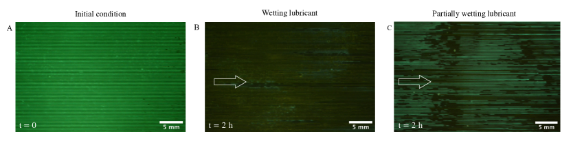
We start by characterizing the lubricant-water interface for the flow configuration Re=9100 (Tab. 1) in the presence of the partially wetting and wetting LISs (Tab. 2). Figure 3A shows the wetting LIS at the beginning of the experiment where the grooves are filled with lubricant (green). The initial state of the partially wetting LIS looks exactly the same. We observed different states of two LISs after approximately 2 hours exposure to the turbulent flow. The wetting LIS – which adheres to the established design principles where the lubricant fully wets the substrate – was drained, leaving behind only a thin film at the bottom of the grooves where the flow velocity is very small (Fig. 3B). Lubricant depletion in longitudinal grooves without barriers in a shear flow is expected [21]. For partially-wetting LIS – as illustrated in Fig. 3C – after two hours, 46% of the initial lubricant volume remained in the grooves. This demonstrates that a partially wetting lubricant can resist drainage when exposed to a flow. Somewhat contradictory, the chemically incompatible LIS, which breaks the equilibrium design rule offers a greater resistance to drainage in non-equilibrium conditions. Appendix B provides a more quantitative assesment of the lubricant drainage for different configurations.
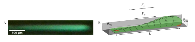
The experiments (SI Movies S2, S3, and S4) of partially wetting LISs reveal that the lubricant-water interface initially breaks up, allowing water to infiltrate the grooves, after which the lubricant forms elongated droplets pinned to the surface (Fig. 4A). At the contact lines, where the water-lubricant-solid phases meet, there is an adhesive force that depends on the physical and chemical heterogeneity of the substrate. The force can be expressed as [22],
as represented in Fig. 4B. This adhesive force acts in the opposite direction to the external hydrodynamic force,
where is the (averaged) shear stress on the lubricant-liquid interface, and is the length of the lubricant droplet. By equating the two forces, we can define the largest possible length of a stationary droplet as
This means that, in the presence of triple-phase contact lines, the adhesive force can resist the imposed shear stress for lubricant droplets of length . Droplets longer than , on the other hand, will be displaced because the shear stress exceeds the pinning force. As we will quantitatively demonstrate in the following sections, the partially wetting LIS has pinned contact lines and sufficiently large CAH to yield stationary lubricant droplets reaching up to 35 mm in length. In contrast, the wetting LIS spreads into a thin film at the bottom of the grooves without well-defined contact lines.
IV Theoretical model of maximum retention length
Having observed significant lubricant retention of partially wetting LIS in turbulent flows, we now develop a model that predicts the maximum droplet length for a given shear stress and contact-angle hysteresis. We consider a long groove that is filled with a lubricant and subjected to a uniform interface shear stress (Fig. 5A). The imposed viscous stress generates a steady and unidirectional lubricant flow in the streamwise direction resulting in a flux given by [21],
where is a geometry-dependent constant (see App. C) and is the lubricant viscosity. For stable retention, there must be a flux in the opposite direction that exactly balances . Assuming that the opposite lubricant flow is driven by a constant pressure gradient , the associated flux can be written as [21],
where is another geometry-dependent constant. The balance of the two fluxes results in,
| (3) |
The pressure gradient arises from the adhesion force at the contact line of a droplet in the groove. The force [23] is defined as
| (4) |
where is a unit vector that is tangent to the liquid-lubricant interface and normal to the contact line. The integration is performed along a closed curve, where the lubricant-liquid-solid phases meet (App. C). We assume a constant angle along the entire contact line of upstream and downstream parts of the droplet, given by and , respectively. Under these assumptions and since the droplet completely wets the side walls of the groove, we obtain
| (5) |
With assumed to change the pressure equally over the projected area in the -plane, we can write,
| (6) |
where is the length of the droplet. By inserting (6) into the flux balance (3), we can define the maximum retention length as,
| (7) |
The constant depends on the substrate geometry, which for longitudinal grooves is given by
Droplets of length are stationary if
| (8) |
as they can induce a sufficient pressure gradient to balance the imposed external shear stress. Droplets with , on the other hand, will move downstream in the groove.
Fig. 5B shows how varies with the advancing and receding contact angles for Pa. We observe that retention lengths of a few millimetres can be obtained from relatively small CAH (). Almost all surfaces exhibit some degree of contact angle hysteresis [24, 25]. Highly smooth surfaces, such as those made of PTFE (polytetrafluoroethylene), typically exhibit low contact angle hysteresis (), while PDMS (polydimethylsiloxane) and Rose-petal type of surfaces can have exceeding [26, 27]. The model developed herein contains the essential ingredients for the CAH-based retention mechanism. We have neglected inertial and gravitational effects in the lubricant and assumed a large viscosity ratio (, which indicates negligible slippage at the lubricant-liquid interface [28]). Furthermore, long-range forces such as van der Waals forces have been neglected, which implies the absence of nanometric precursor films in the grooves.
Previous work [21, 29, 30] have, instead of CAH, introduced physical or chemical barriers in the grooves to generate a shear-resisting pressure gradient. The maximum retention length provided by Wexler et. al. [21] for a lubricant-infused longitudinal groove that terminates in a lubricant reservoir reads,
| (9) |
where approximates the interface curvature at the tail of the droplet. Equation (9) is a special case of (7) with , since the interface curvature is a consequence of the pinning force.
V Retention distribution and numerical simulations
| 9100 | 0.9 | 5.8 | 35.8 | 32.2 0.2 | 54 |
|---|---|---|---|---|---|
| 13000 | 1.3 | 10.4 | 19.8 | 14.6 0.2 | 71 |
| 15600 | 1.6 | 14.0 | 14.7 | 12.2 0.2 | 82 |
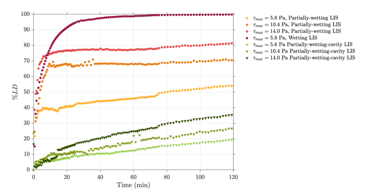
To verify that stationary droplets satisfy (8), we now consider water channel experiments at higher flow velocities (Re=13000 and Re=15600) using the partially wetting LIS (Tab. 3). In a turbulent flow, the streamwise wall-shear stress (WSS) near the lubricant-liquid interface fluctuates, resulting in intermittent peaks that can be up to 80% higher than the mean wall-shear stress [31, 32]. Since the time scale of the fluctuations is on the order of milliseconds, we expect that all lubricant-liquid interfaces will be exposed to the peak WSS within a 2-hour interval. Consequently, the pinning force must be sufficiently large to withstand the maximum WSS. Therefore, when evaluating (7) for turbulent flows, the shear stress is approximated by , where is the streamwise WSS fluctuations. The maximum WSS can be estimated from,
where is the root-mean-square of the streamwise WSS. The approximations above are based on relations and PDFs obtained from experiments [31] and numerical simulations [32]. Using in (7), we calculated the predicted maximum retention lengths which range from 35.8 mm for the lowest flow speed to 14.7 mm for the fastest flow speed (Tab. 3). The corresponding measured maximum retention lengths, , range from 32.2 mm to 12.2 mm. The agreement with the predictions is remarkable, considering that we have not used empirical fitting parameters despite dealing with a turbulent flow.
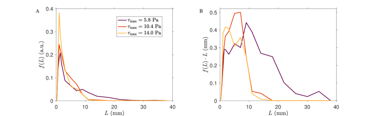
Lubricant droplets with maximum lengths are however rare. The stationary LIS has many smaller droplets that can generate higher pressure gradients for opposing the shear stress (as indicated by Eq. 6). To quantify the distribution of droplet lengths in the stationary state, we calculated the probability density function (Fig. 6A). We observe that droplets with a length of approximately 1.5 mm appear most frequently across all shear stress values. Droplets with lengths greater than 10 mm have a low occurrence rate, particularly at high shear stresses.
While short droplets dominate in quantity, longer droplets contribute significantly to overall lubricant retention. The total volume of lubricant retained in the stationary LIS can be approximated by , where is the constant cross-sectional area of the groove, the number of retained droplets in the surface and is the mean lubricant length, which is given by
| (10) |
This indicates that the total lubricant volume depends on the product, , shown in Fig. 6(B). The contribution to is fairly equal from droplets with lengths ranging from mm to mm for two cases of high shear stress, and with lengths between mm and mm for the lower shear stress case. This implies that short and long droplets contribute equally to the volume of lubricant that is retained by the surface.
.
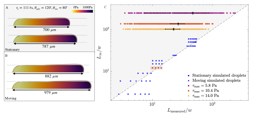
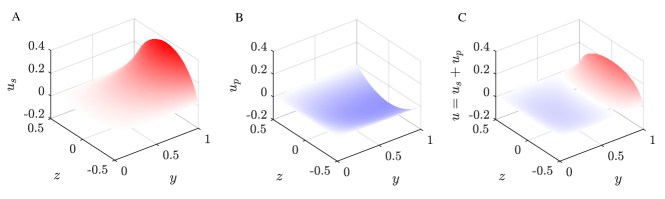
The theoretical retention length is the upper limit of a range of droplet lengths that exist in turbulence. To demonstrate that the theoretical model is predictive when excluding the turbulent fluctuations, we have performed a set of numerical simulations using the open-source software OpenFOAM [33]. See Appendix D for details of the numerical method. We considered the laminar shear (Couette) flow over a single lubricant-infused groove, with the same density and viscosity for the infused and external fluids. We modelled CAH by pinning the contact line when the apparent contact angle is within the hysteresis window ; otherwise, the contact line moves with a prescribed constant contact angle. The computational domain had dimensions with a groove size ratio , similar to our experiments. We imposed a constant and , and then gradually increased the volume of a lubricant droplet in the groove.
Figs. 7A and B show how the lubricant droplet is deformed by the shear stress when . The pressure difference between the front and back end of the droplet is induced by contact-line force that pins the interface to the surface, causing the interface away from the surface to deform. The downstream and upstream contact lines dominate the adhesion force, so is the same for droplets of all sizes. However, the pressure gradient () is only sufficiently strong to withstand the imposed shear stress when the droplet length is smaller than a critical value. Our numerical simulations show that the droplet is stationary below m, but is moving when m (Figs. 7A and B). The maximum possible droplet length obtained from (7) is m, which lies in between the stationary and the moving droplets.
The numerical and experimental results are collected in a retention map in Fig. 7C. The map shows the predicted retention lengths normalized by the groove width, , plotted against the measured retention lengths, . The dashed line represents , the gray region marks (stationary droplets) while the white region marks (moving droplets). The latter case indicates that the resistance due to contact line hysteresis is unable to withstand the applied shear stress. All the measured lubricant droplets in the turbulent channel flow experiments – evaluated after 2 hours – fall into the stable grey region of the map. The large filled markers represent the mean of the distributions of the retention lengths, and the horizontal error bars represent their variance. We note that the mean and maximum values of the distributions decrease with a slope similar to the stability boundary. This indicates consistency in the scaling of the retention lengths with the shear stress. The numerical simulations allow varying the shear stress and CAH over a wide range ( Pa and ). We observe a quantitative agreement between the numerical simulations and the theory, where nearly all the stationary (circles) and moving (crosses) lubricant droplets fall into the stable and unstable regimes, respectively. This also confirms that the retention length in unidirectional flows is quantitatively given by (7) while the expression serves as an upper limit in the presence of turbulence.
VI Discussion
For liquid-repellent and anti-adhesive applications, where the external environment is near equilibrium, LISs rely on chemical compatibility to keep the lubricant robustly trapped in the microstructures. Expression (2) determines lubricant-solid compatibility specifically for lubricant spreading in streamwise grooves [19], but can be generalized to any surface texture [13]. Condition (2) is often fulfilled by tuning the surface chemistry, for example, by depositing a layer of octadecyltrichlorosilane (OTS) onto silicon surfaces [12].
Our findings provide a starting point for developing chemistry-free lubricant-infused surfaces for applications where the external environment is continuously flowing. In Fig. 8A, we present a LIS design featuring cavities of length 1.5 mm and with the same width and height as the previous longitudinal grooves. The length of the cavities correspond to half of the average drop length measured at the flow case 3. For the partially wetting lubricant, we obtained retention (Fig. 8B) after 2 hours in the presence of turbulent flow (). The depletion was due to the initial dewetting (Fig. 10). This demonstrates that a LIS, where (2) is not satisfied, can stably trap lubricant droplets if
| (11) |
To provide a design criterion for a general microstructured surface, we define a capillary number as , which represents the balance between the external viscous force and the capillary force within a surface cavity. The condition in (11) can be recast as a non-dimensional criterion for a drop to remain pinned in the microstructured surface,
| (12) |
where
| (13) |
and
| (14) |
The critical number, , is a function of the surface microstructure properties and independent of the flow. The coefficient in (14) takes into account three essential surface features. The ratio – which can be obtained by solving Stokes equations in a unit cell of the texture – accounts for the relative ease for which lubricant flux is generated in the texture from imposed pressure gradient () and shear stress (). Moreover, is inversely proportional to the streamwise-averaged groove width, , since narrower structures result in less exposed interfacial area to external shear stress. Finally, the integral in (14) represents the total length for which the contact line force has a component in the -direction. An analogue condition to (12) exists for the configuration where a drop partially wets an inclined surface. The condition reads , where is the Bond number and gravity is the driving external force [22].
As shown by Wexler et. al. [21], when both conditions (2) and (12) are fulfilled, the lubricant spontaneously wets the textured surface and retention is enforced through distinct physical or chemical barriers that generate a resisting Laplace pressure gradient. Such self-healing LIS [1, 2] are useful in applications that require high precision control of multiple transport processes, such as microfluidic devices, batteries, microprocessors and micro-heat exchangers. We have shown that significant retention in the presence of a flow can be achieved through a resistive pinning force without satisfying the equilibrium criterion (2). This comes, however, at the cost of a loss (10%-20% in our experiments) of lubricant caused by a rapid initial dewetting process. In many large turbulent flow systems, partially lubricated surfaces may still offer significant functionality. Examples include marine systems, food processing units, medical devices and thermal systems. Chemistry-free LIS would significantly increase the possible choices of lubricants for these applications by circumventing the difficulty in fabricating and sustaining large chemically-tuned surfaces. Additionally, chemistry-free LIS would address the environmental concern when using large volumes of hydrophobic polymers and other inert lubricants, which degrade very slowly in nature.
In summary, we have investigated a new retention mechanism of lubricant-infused surfaces that relies on contact-angle hysteresis of a substrate. We found that a partially wetting lubricant that naturally develops triple-phase contact lines can withstand relatively large shear stress in dynamic environments. We have derived an expression of the maximum possible length of lubricant droplets, , and validated the expression in laminar and turbulent flows. Our study offers the prospect of a new class of LIS for submerged conditions. This can contribute to developing large-scale lubricated surfaces that remain clean and energy-efficient in harsh flow environments.
Acknowledgements
We acknowledge support from Kunt and Alice Wallenberg foundation (KAW 2016.0255) and the Swedish Foundation for Strategic Research (FFL15:0001). We thank Susumu Yada and Saumey Jain for helping with surface fabrication. Access to the computational resources used for this work were provided by the Swedish National Infrastructure for Computing (SNIC).
Author contributions
Sofia Saoncella (SoSa) performed experiments, Johan Sundin (JS) developed the theory and So Suo (SiSu) performed numerical simulations. Agastya Partikh (AP), SoSa, Marcus Hultmark (MH) and Shervin Bagheri (SB) constructed the water channel facility. SoSa, SiSu, JS, Wouter Metsola van der Wijngaart (WmW) and Fredrik Lundell (FL) and SB analyzed data. SoSa and SB wrote the paper with feedback from all authors.
Appendix A Substrate fabrication and characterization
The solid substrates of the LISs are fabricated with a soft lithographic method from Ostemer 322 (Mercene Labs, Stockholm, Sweden), Off-Stoichiometry-Thiol-Ene resin (OSTE). A flat layer of resin with size is cured on a black plastic sheet by exposure to UV radiation for . A second layer of resin is then prepared and cured for with a geometric pattern by filtering the UV light through a photomask decorated with the desired 2D geometry, in this case, longitudinal grooves. The depth of the grooves is determined by the thickness of spacers on which the photomask rests. The uncured resin is washed from the sample in an ultrasonic bath of PGMEA (Propylene-Glycol-Methyl-Ether-Acetate, Sigma-Aldrich) and dried with compressed air for three times. Finally, the surface is cured in an oven at C for one hour. The hardened resin can then be coated to modify its surface energy. The low-energy substrate used for the partially wetting LIS was left uncoated, while the high-energy substrate, used for the wetting LIS, was spray-coated with a super water-repellent coating (HYDROBEAD-T). The final substrate is composed of four parts fabricated as described and mounted adjacently.
The contact angle of a drop of lubricant on the samples immersed in water are measured using the sessile drop method in an inverted setup configuration. Since the density of hexadecane is lower than that of water, the lubricant drop is generated from a thin needle (diameter , Hamilton, Gauge 30, point style 3) placed underneath the solid substrate immersed in water. As the drop is generated, buoyancy lifts it toward the sample surface, and the needle holding the drop is gradually brought closer to the surface until contact is made. The drop has a volume of about and the oil is pumped or withdrawn by a syringe pump (New Era Pump Systems Inc., NE-4000) at a flow rate of to measure advancing and receding angles, respectively (Fig. 9). The angle right before the contact line starts to advance (recede) is defined as the advancing (receding ) contact angle. The contact angles measurements were repeated with ten drops for each case in different positions on the substrate; the reported angles correspond to the average values.
Appendix B Evaluation of lubricant drainage
The percentage of lubricant drainage with respect to the initial condition is defined as
where represents the volume of lubricant (per unit area) that infuses the grooves, evaluated at time . In the expression above, denotes the initial time. The quantity is extracted from the acquired images, assuming that the height of the lubricant in the groove is directly proportional to the pixel intensity. Therefore, the lubricant volume per unit area is computed as the sum of pixel intensities at time ,
| (15) |
The temporal evolution of lubricant drainage for both the wetting LIS and partially wetting LIS is shown in Fig. 10. After two hours, the wetting LIS (dark red markers) is completely drained (). Within the first 25 minutes, approximately 90% of the lubricant volume is lost due to shear-driven drainage. This is followed by slower drainage of a thin film at the walls of the groove. For all partially wetting lubricants in longitudinal grooves without transversal barriers (indicated by the red, dark orange, and orange markers), finite retention is observed (). As anticipated by the presented theory, lubricant depletion increases with the shear stress. There is a decay within the first 10 minutes caused by the disruption of the liquid-liquid interface induced by turbulent fluctuations. This allows water to penetrate and partially displace the lubricant in the grooves, resulting in the loss of lubricant droplets entrained in the bulk. The remaining lubricant forms elongated droplets that remain essentially stationary. Partially wetting lubricants in cavities (depicted by the green symbols) exhibit a considerably slower rate of drainage. The accompanying supplementary movies (Movie S1-Movie S7) demonstrate a very slow movement of partially wetting configurations and a slow change in fluorescence intensity. Both these effects contribute to not fully saturating.
Appendix C Analytical description of flow field
The Stokes equations are solved analytically to describe the fluid motion in the lubricant. We consider a completely oil-filled groove subjected to a uniform (constant) fluid-fluid interface shear stress . The wall-normal coordinate is at the bottom, while the spanwise coordinate is at the centerline of the groove.
C.1 Problem definition
Following Wexler et al. [34], it is assumed that the flow is unidirectional, with the streamwise velocity satisfying
| (16) |
where is a constant pressure gradient inside the groove. The boundary conditions are
| (17a) | |||||||
| (17b) | |||||||
| (17c) | |||||||
Since Eq. 16 is linear, we can consider as a superposition of two solutions and , driven by the imposed shear stress and the pressure gradient, respectively. They satisfy
| (18) |
| (19a) | |||||||
| (19b) | |||||||
| (19c) | |||||||
and
| (20) |
| (21a) | |||||||
| (21b) | |||||||
| (21c) | |||||||
C.2 Solution by separation of variables
C.2.1 Shear-driven flow
Starting with , we assume
| (22) |
Eq. 18 implies
| (23) |
where is a constant. We consider , for which the solution for is
| (24) |
for coefficients and . We are only interested in solutions symmetric with respect to , giving . The boundary conditions (19a) equal , giving , where . The solution for can be written
| (25) |
for coefficients and . The boundary condition (19b) implies , giving . An expression for is therefore
| (26) |
for coefficients .
The inhomogeneous boundary condition (19c) must also be satisfied. First, we take the derivative of Eq. 26, to obtain,
| (27) |
Then, we expand the constant function over the interval in a Fourier series as (see e.g. [36])
| (28) |
assuming that its wavelength is . Matching Eqs. 27 and 28, we have
| (29) |
and thus,
| (30) |
To compute the flux, we integrate over the cross-section. We have that
| (31) |
and
| (32) |
Hence,
| (33) | |||||
In the above expression, we used that (see e.g. [36])
| (34) |
We also introduced the geometrical resistance constant as a function of . An alternative, but equivalent, expression for was given by [34],
| (35) |
C.2.2 Pressure-driven flow
We now move on to finding for the inhomogeneous system given Eq. 20. We assume a solution similar to Eq. 26,
| (36) |
with functions . Similar as for in Eq. 28, we can write
| (37) |
Eq. 20 then results in
| (38) |
The general solutions can be found by adding a particular solution and a homogeneous solution to fulfil the boundary conditions,
| (39) |
A particular solution is simply given by
| (40) |
The general solution to the homogeneous equation is equivalent to Eq. 26, so that
| (41) | |||||
for coefficients and . The boundary conditions on the side walls are fulfilled (eq. 21a). The bottom wall no-slip condition (21b) and the top wall no-shear condition (21c) imply,
| (42) |
respectively. The complete solution is
| (43) | |||||
To evaluate the corresponding flux, we use that the integral
| (44) |
Eqs. 31, 32, and 44 give the flux
| (45) | |||||
where is a geometrical resistance constant. An alternative expression, but equivalent, for was given by Wexler et al. [34],
| (46) |
C.3 Required pressure drop
For there to be no drainage of groove liquid, the fluxes need to balance,
| (47) |
The expression for the fluxes, (33) and (45), result in
| (48) |
If the pressure gradient is less than this value, there is drainage of liquid. An example of flow fields with balancing shear stress and pressure gradient are shown in Fig. 11.
C.4 Droplet hysteresis
The adhesion force is defined as
| (49) |
Here, is a unit vector that is tangent to the liquid-lubricant interface and normal to the contact line. We may express this vector in terms of normals of the solid surface and interface. The interfacial tension force per unit length at the contact line projected onto the solid is . The angle is the contact angle which also is the angle between the interface normal at the contact line and the solid normal ( and , respectively). The projected force is in the direction of the projected interface normal (where points out from the droplet). The net contribution from the surface tension force acting on the droplet at the contact line in the streamwise direction is, therefore
| (50) |
where is the streamwise unit vector. We assume that on the upstream side of the droplet and on the downstream, which are the simplest possible assumptions. Downstream and upstream contact lines at the bottom of the groove are perfectly perpendicular to the streamwise flow ( give a contribution
| (51) |
which is used here. We assume that the contact line on the walls goes all the way from the bottom to the top of the grooves ( to ). On the side walls, = , where is the contact line tangent unit vector in the direction of integration. Looking at the wall on the dowstream side where the integral starts from the bottom of the groove and goes to the top ( = ),
| (52) | |||||
by the gradient theorem. The forces from the other side-wall parts of the contact line can be computed in analog. The total contribution is
| (53) |
Hence,
| (54) |
This net force acting in the negative streamwise direction is assumed to give rise to interface curvature and a corresponding pressure gradient over the droplet. The reference pressure of the external flow is assumed to be constant, and the pressure differences over the interface at the upstream and downstream part ( and , respectively) are given by the curvature. With assumed to change the pressure equally over the projected area in the -plane, the effective pressure gradient can be written
| (55) |
for a droplet length . Together with the flux balance (48), the maximum stationary-state droplet length becomes
| (56) |
Appendix D Numerical model
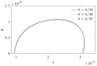
We consider a single lubricant droplet exposed to a fully developed shear flow. The flow domain has the size , where , , represent the streamwise, wall-normal and spanwise directions, respectively. We consider a half pitch in the spanwise direction – i.e., from the centreline of a groove to the centerline of a crest – and impose symmetry boundary conditions on both sides. Along the streamwise direction, a periodic boundary condition is imposed. At the top side, a moving wall boundary with a constant streamwise velocity is set. The streamwise-aligned groove has a rectangular cross-section, and its size ratio is . For computational feasibility, the droplet length is limited to , which is shorter than the lengths observed in experiments. Therefore, we increase the shear stress ( Pa) or decrease the hysteresis () to find the boundary between the regimes where droplets are stationary and moving. The numerical scheme in OpenFOAM employs a geometric VOF-based method for interface capturing [37, 38]. At solid walls, contact angle hysteresis is implemented by using the Robin boundary condition (see [39] for details). Finally, the flow domain is meshed with a uniform cubic cell, and the chosen cell size has been confirmed to produce convergent results through a sensitivity analysis (Fig. 12). The lubricant droplet reaches a steady state, i.e., stably moving or retaining, within , and the final state of the droplet is recorded at .
References
- Wong et al. [2011] T. S. Wong, S. H. Kang, S. K. Tang, E. J. Smythe, B. D. Hatton, A. Grinthal, and J. Aizenberg, Bioinspired self-repairing slippery surfaces with pressure-stable omniphobicity, Nature 477, 443 (2011).
- Lafuma and Quéré [2011] A. Lafuma and D. Quéré, Slippery pre-suffused surfaces, EPL 96, 10.1209/0295-5075/96/56001 (2011).
- Epstein et al. [2012] A. K. Epstein, T.-S. Wong, R. A. Belisle, E. M. Boggs, and J. Aizenberg, Liquid-infused structured surfaces with exceptional anti-biofouling performance, PNAS 109, 13182 (2012).
- Zouaghi et al. [2017] S. Zouaghi, T. Six, S. Bellayer, S. Moradi, S. G. Hatzikiriakos, T. Dargent, V. Thomy, Y. Coffinier, C. Andre, G. Delaplace, et al., Antifouling biomimetic liquid-infused stainless steel: application to dairy industrial processing, ACS applied materials & interfaces 9, 26565 (2017).
- Charpentier et al. [2015] T. V. Charpentier, A. Neville, S. Baudin, M. J. Smith, M. Euvrard, A. Bell, C. Wang, and R. Barker, Liquid infused porous surfaces for mineral fouling mitigation, Journal of colloid and interface science 444, 81 (2015).
- Solomon et al. [2014] B. R. Solomon, K. S. Khalil, and K. K. Varanasi, Drag reduction using lubricant-impregnated surfaces in viscous laminar flow, Langmuir 30, 10970 (2014).
- Pakzad et al. [2022] H. Pakzad, A. Nouri-Borujerdi, and A. Moosavi, Drag reduction ability of slippery liquid-infused surfaces: A review, Progress in Organic Coatings 170, 106970 (2022).
- Fu et al. [2017] M. K. Fu, I. Arenas, S. Leonardi, and M. Hultmark, Liquid-infused surfaces as a passive method of turbulent drag reduction, Journal of Fluid Mechanics 824, 688 (2017).
- Van Buren and Smits [2017] T. Van Buren and A. J. Smits, Substantial drag reduction in turbulent flow using liquid-infused surfaces, Journal of Fluid Mechanics 827, 448 (2017).
- Lee et al. [2019] S. J. Lee, H. N. Kim, W. Choi, G. Y. Yoon, and E. Seo, A nature-inspired lubricant-infused surface for sustainable drag reduction, Soft Matter 15, 8459 (2019).
- Sundin et al. [2022] J. Sundin, U. Ciri, S. Leonardi, M. Hultmark, and S. Bagheri, Heat transfer increase by convection in liquid-infused surfaces for laminar and turbulent flows, Journal of Fluid Mechanics 941, 10.1017/jfm.2022.279 (2022).
- Smith et al. [2013] J. D. Smith, R. Dhiman, S. Anand, E. Reza-Garduno, R. E. Cohen, G. H. McKinley, and K. K. Varanasi, Droplet mobility on lubricant-impregnated surfaces, Soft Matter 9, 1772 (2013).
- Preston et al. [2017] D. J. Preston, Y. Song, Z. Lu, D. S. Antao, and E. N. Wang, Design of lubricant infused surfaces, ACS Applied Materials & Interfaces 9, 42383 (2017).
- Villegas et al. [2019] M. Villegas, Y. Zhang, N. A. Jarad, L. Soleymani, and T. F. Didar, Liquid-infused surfaces: A review of theory, design, and applications, ACS Nano 13, 8517 (2019).
- Li et al. [2019] J. Li, E. Ueda, D. Paulssen, and P. A. Levkin, Slippery lubricant-infused surfaces: Properties and emerging applications, Advanced Functional Materials 29, 10.1002/adfm.201802317 (2019).
- Baumli et al. [2021] P. Baumli, M. D’Acunzi, K. I. Hegner, A. Naga, W. S. Wong, H. J. Butt, and D. Vollmer, The challenge of lubricant-replenishment on lubricant-impregnated surfaces (2021).
- Peppou-Chapman et al. [2020] S. Peppou-Chapman, J. K. Hong, A. Waterhouse, and C. Neto, Life and death of liquid-infused surfaces: a review on the choice, analysis and fate of the infused liquid layer., Chemical Society reviews 49, 3688 (2020).
- Dean [1978] R. B. Dean, Reynolds number dependence of skin friction and other bulk flow variables in two-dimensional rectangular duct flow, Journal of Fluids Engineering 100, 215 (1978).
- Quéré [2008] D. Quéré, Wetting and roughness, Annual Review of Materials Research 38, 71 (2008).
- Eral et al. [2013] H. B. Eral, D. ’t Mannetje, and J. M. Oh, Contact angle hysteresis: a review of fundamentals and applications, Colloid and polymer science 291, 247 (2013).
- Wexler et al. [2015a] J. S. Wexler, I. Jacobi, and H. A. Stone, Shear-driven failure of liquid-infused surfaces, Physical Review Letters 114, 168301 (2015a).
- Furmidge [1962] C. Furmidge, Studies at phase interfaces. i. the sliding of liquid drops on solid surfaces and a theory for spray retention, Journal of Colloid Science 17, 309 (1962).
- de Gennes et al. [2004] P.-G. de Gennes, F. Brochard-Wyart, and D. Quéré, Capillarity and Wetting Phenomena: Drops, Bubbles, Pearls, Waves (Springer, New York, NY, 2004).
- Samuel et al. [2011] B. Samuel, H. Zhao, and K.-Y. Law, Study of wetting and adhesion interactions between water and various polymer and superhydrophobic surfaces, The Journal of Physical Chemistry C 115, 14852 (2011).
- Laroche et al. [2023] A. Laroche, A. Naga, C. Hinduja, A. A. Sharifi, A. Saal, H. Kim, N. Gao, S. Wooh, H.-J. Butt, R. Berger, et al., Tuning static drop friction, Droplet , 2:e42 (2023).
- Allred et al. [2019] T. Allred, J. Weibel, and S. Garimella, The petal effect of parahydrophobic surfaces offers low receding contact angles that promote effective boiling, International Journal of Heat and Mass Transfer 135, 403 (2019).
- Bhushan and Nosonovsky [2010] B. Bhushan and M. Nosonovsky, The rose petal effect and the modes of superhydrophobicity, Philosophical Transactions of the Royal Society A: Mathematical, Physical and Engineering Sciences 368, 4713 (2010).
- Liu et al. [2016] Y. Liu, J. S. Wexler, C. Schönecker, and H. A. Stone, Effect of viscosity ratio on the shear-driven failure of liquid-infused surfaces, Phys. Rev. Fluids 1, 074003 (2016).
- Wexler et al. [2015b] J. S. Wexler, A. Grosskopf, M. Chow, Y. Fan, I. Jacobi, and H. A. Stone, Robust liquid-infused surfaces through patterned wettability, Soft Matter 11, 5023 (2015b).
- Fu et al. [2019] M. K. Fu, T.-H. Chen, C. B. Arnold, and M. Hultmark, Experimental investigations of liquid-infused surface robustness under turbulent flow, Experiments in Fluids 60, 1 (2019).
- Alfredsson et al. [1988] P. H. Alfredsson, A. V. Johansson, J. H. Haritonidis, and H. Eckelmann, The fluctuating wall-shear stress and the velocity field in the viscous sublayer, The Physics of fluids 31, 1026 (1988).
- Cheng et al. [2020] C. Cheng, W. Li, A. Lozano-Durán, and H. Liu, On the structure of streamwise wall-shear stress fluctuations in turbulent channel flows, Journal of Fluid Mechanics 903, A29 (2020).
- Roenby et al. [2016] J. Roenby, H. Bredmose, and H. Jasak, A computational method for sharp interface advection, Royal Society open science 3, 160405 (2016).
- Wexler et al. [2015c] J. S. Wexler, A. Grosskopf, M. Chow, Y. Fan, I. Jacobi, and H. A. Stone, Robust liquid-infused surfaces through patterned wettability, Soft Matter 11, 5023 (2015c).
- Shah and London [1978] R. K. Shah and A. L. London, Laminar Flow Forced Convection in Ducts (Academic Press, 1978).
- Råde and Westergren [1999] L. Råde and B. Westergren, Mathematics Handbook for Science and Engineering (Springer, 1999).
- Gamet et al. [2020] L. Gamet, M. Scala, J. Roenby, H. Scheufler, and J.-L. Pierson, Validation of volume-of-fluid openfoam® isoadvector solvers using single bubble benchmarks, Computers & Fluids 213, 104722 (2020).
- Scheufler and Roenby [2019] H. Scheufler and J. Roenby, Accurate and efficient surface reconstruction from volume fraction data on general meshes, Journal of Computational Physics 383, 1 (2019).
- Linder [2015] N. Linder, Numerical simulation of complex wetting, PhD thesis (Technische Universität, 2015).