HiMTM: Hierarchical Multi-Scale Masked Time Series Modeling for Long-Term Forecasting

Abstract

Time series forecasting is crucial and challenging in the real world. The recent surge in interest regarding time series foundation models, which cater to a diverse array of downstream tasks, is noteworthy. However, existing methods often overlook the multi-scale nature of time series, an aspect crucial for precise forecasting. To bridge this gap, we propose HiMTM, a hierarchical multi-scale masked time series modeling method designed for long-term forecasting. Specifically, it comprises four integral components: (1) hierarchical multi-scale transformer (HMT) to capture temporal information at different scales; (2) decoupled encoder-decoder (DED) forces the encoder to focus on feature extraction, while the decoder to focus on pretext tasks; (3) multi-scale masked reconstruction (MMR) provides multi-stage supervision signals for pre-training; (4) cross-scale attention fine-tuning (CSA-FT) to capture dependencies between different scales for forecasting. Collectively, these components enhance multi-scale feature extraction capabilities in masked time series modeling and contribute to improved prediction accuracy. We conduct extensive experiments on 7 mainstream datasets to prove that HiMTM has obvious advantages over contemporary self-supervised and end-to-end learning methods. The effectiveness of HiMTM is further showcased by its application in the industry of natural gas demand forecasting.

1 Introduction

Time series is an important data type that is widely collected from finance, the Internet of Things (IoT), and wearable devices Esling and Agon (2012); Wen et al. (2023). Analysis and modeling of time series data play crucial roles such as financial analysis, energy planning, and human health assessment Chen et al. (2023c); Eldele et al. (2023). Time series forecasting Lim and Zohren (2021); Benidis et al. (2022), in particular, has garnered widespread attention in recent years. Researchers have introduced a range of methods, starting from traditional statistical approaches to contemporary deep learning models. Deep learning methods stand out due to their ability to learn temporal dependencies from large-scale time series data, eliminating the need for labor-intensive data preprocessing and feature engineering Du et al. (2021).

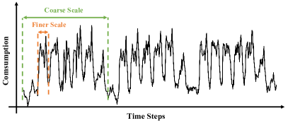
Figure 1: Illustration of the multi-scale phenomenon on the Electricity dataset.

In recent years, self-supervised representation learning Baevski et al. (2022); Ericsson et al. (2022) has made substantial advancements in computer vision (CV) and natural language processing (NLP), leading to a growing interest in learning universal representations for time series and its application in various downstream tasks Ma et al. (2023); Jin et al. (2023); Zhang et al. (2023b). Self-supervised learning such as contrastive learning He et al. (2020); Yue et al. (2022) and masked modeling Zhang et al. (2023a); Dong et al. (2023) emphasizes the extraction of meaningful knowledge from large, unlabeled datasets. Our work primarily focuses on the application of masked modeling to time series data, referred to as masked time series modeling (MTM) Dong et al. (2023). The key principle of this approach is to optimize the model by learning to reconstruct the masked content based on the observable parts He et al. (2022); Cheng et al. (2023).

While masked time series modeling has achieved significant improvements in various downstream tasks such as classification and forecasting Ma et al. (2023), it still encounters certain challenges. One of the primary issues is its inability to capture multi-scale information Shabani et al. (2022); Zhang et al. (2023c), which is crucial for time series modeling. For example, the consumption of energy such as electricity and natural gas usually exhibits patterns on different time scales, including hours, days, months, and even years. Figure 1 depicts the multi-scale characteristics of the Electricity dataset Wu et al. (2021), highlighting that the finer scale captures short-term patterns, while the coarse scale encapsulates long-term trends. Therefore, modeling multi-scale dependencies is crucial for time series tasks. Some related studies Cui et al. (2016); Du et al. (2023); Chen et al. (2023a) have also demonstrated the importance of multi-scale information for time series analysis. Nevertheless, integrating the ability to extract multi-scale features into masked time series modeling poses several critical challenges:

• Firstly, the vanilla transformer design only processes fixed-scale tokens, and masked modeling typically employs a random masking approach. Additionally, the encoder’s potential may not be fully realized as the learned representations are subject to further optimization during the decoding phase.

• Secondly, current masked time series modeling methods are centered on reconstruction at a consistent, fixed scale. This approach is insufficient for multi-scale modeling, as the singular focus on fixed-scale reconstruction restricts the ability to provide diverse, multi-stage guidance signals for better characterization of time series.

• Thirdly, following the extraction of multi-scale features, many methods resort to either concatenation or global pooling of these features. This approach, however, falls short of effectively establishing significant correlations between features across various scales.

To tackle these challenges, we propose HiMTM, a novel hierarchical multi-scale masked time series modeling framework designed for long-term forecasting. This is, to our knowledge, the pioneering effort to integrate multi-scale feature extraction into masked time series modeling. HiMTM encompasses four key components, including hierarchical multi-scale transformer (HMT), decoupled encoder-decoder (DED), multi-scale masked reconstruction (MMR), and cross-scale attention fine-tuning (CSA-FT). In summary, the main contributions of this paper are outlined as follows:

• HMT: We introduce a hierarchical multi-scale transformer, equipped with the hierarchical patching partition strategy. This approach involves segmenting finer-grained patches within coarser-grained ones, which then serve as the input for HMT, enhancing its ability to process time series exhibiting multi-scale characteristics.

• DED: In our method, the encoder is designed to process visible patches to extract temporal dependencies. Conversely, the decoder focuses on masked queries, aiming to reconstruct the masked segments based on the encoder’s representations. This distinct separation enables the encoder to concentrate on feature extraction, while the decoder addresses the pretext task.

• MMR: We implement a decoder at each level of the encoder hierarchy, dedicated to reconstructing the masked parts. This multi-hierarchical approach offers varied levels of supervision signals, thereby more effectively guiding the pre-training process.

• CSA-FT: In the fine-tuning stage, we introduce cross-scale attention, enabling the model to integrate dependencies among representations at different scales.

2 Related Works

2.1 Time Series Forecasting

Over the years, time series forecasting has consistently been a hot topic in both industry and academia. Recently, researchers have attempted to apply transformers to capture long-range dependencies and have achieved excellent performance Wen et al. (2022); Li et al. (2023a). Autoformer Wu et al. (2021) borrows the decomposition and autocorrelation mechanisms commonly used in time series analysis to achieve efficient and accurate long-term forecasting. PatchTST Nie et al. (2022) divides time series into several patches to retain more semantic information and significantly reduce computational complexity.

However, deep learning requires a large amount of data to achieve satisfactory results and often performs poorly across domains. Self-supervised learning aims to learn knowledge from large-scale multi-domain unlabeled data and benefit different downstream tasks. Depending on the pretext task, it can be broadly classified into contrastive learning He et al. (2020); Grill et al. (2020); Zheng et al. (2023) and masked modeling He et al. (2022); Shao et al. (2022); Liu et al. (2023). These techniques have demonstrated their effectiveness in CV and NLP, enabling the unsupervised learning of representations that can subsequently be applied to diverse downstream tasks. Although new challenges are brought to self-supervised learning due to the uniqueness of time series, we still find that relevant research is beginning to emerge. This indicates a growing interest in harnessing self-supervised learning to address the distinctive characteristics and complexities of time series.

2.2 Masked Time Series Modeling

Masking modeling was originally popular in the field of NLP and has recently demonstrated outstanding performance in various domains, including CV, audio, and point cloud Pang et al. (2022); Zhang et al. (2023a). MAE He et al. (2022) implements visual representation learning by masking partial patches of the input image and reconstructing missing pixels. CAE Chen et al. (2023b) points out that masked image modeling should separate representation learning and pretext tasks as much as possible to drive the encoder to learn better features.

For time series tasks, TimeMAE Cheng et al. (2023) proposes representation learning for time series classification through two pretext tasks: masked codeword classification and masked representation regression. SimMTM Dong et al. (2023) incorporates manifold learning into masked time series modeling. Masked parts are reconstructed by weighted aggregation of multiple neighbors outside the manifold. However, existing masked time series modeling does not take into account the multi-scale information, which is crucial for time series forecasting.

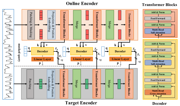
Figure 2: The overall architecture of HiMTM.

3 Method

3.1 Overall Architecture

The overall architecture of HiMTM is shown in Figure 2. The online encoder and the target encoder are both hierarchical multi-scale transformers. The difference is that the online encoder inputs visible patches for multi-scale feature extraction. The target encoder inputs the masked patches, providing multi-stage guidance signals for the pre-training. At each hierarchy, HiMTM utilizes the output of the previous hierarchy or raw time series data as its input. We add a decoder after each hierarchy of encoders to reconstruct the masked parts. In particular, the decoder applies a transformer with cross-attention, forcing the encoder to concentrate on feature extraction, while the decoder focuses on the reconstruction task.

3.2 Hierarchical Multi-scale Transformer

We designed a hierarchical multi-scale transformer to capture time series representation at different scales, making it well-suited for masked time series modeling. The network structure can be seen from the online encoder and target encoder in Figure 2. Specifically, HMT introduces a new hierarchical patch partitioning strategy. After each hierarchy of HMT (except the top hierarchy), the representations of two adjacent (finer-grained) patches are merged to obtain a coarser-grained patch. They are then fed into the next hierarchy to capture the dependencies between coarser-grained representations. This process can be expressed as follows:

$$\mathbf{Z}^{L+1}=\text{Hierarchy}^{L+1}(\mathbf{Z}^{L}),$$ (1)

and

$$\mathbf{Z}^{L}=\left\{\begin{aligned} &\text{Patch\_Embed}(\mathbf{X}),&\text{if }L=1,\\ &\text{Merge}(\mathbf{Z}^{L-1}),&\text{if }L>1,\\ \end{aligned}\right.$$ (2)

where $\mathbf{X}$ denotes the time series sample. $\mathbf{Z}^{L}$ represents the output of HMT at layer $L$. After feature extraction at each hierarchy, we merge two adjacent patches into a coarser-grained patch via Merge (implemented through a fully connected network). The core of the transformer is to capture long-range dependencies through a multi-head attention mechanism (MSA), which receives query $\mathbf{Q}$, key $\mathbf{K}$, and value $\mathbf{V}$ as input and outputs updated features. The specific details can be described as follows:

$$\text{MSA}(\mathbf{Q},\mathbf{K},\mathbf{V})=\text{Concat}(\text{head}_{1},...,\text{head}_{h})\mathbf{W}^{O},$$ (3)

where $h$ denotes the number of heads in the attention layer. Concat means concatenation the outputs of the attention of $h$ heads. Finally, a learnable projection layer $\mathbf{W}^{O}$ is employed to produce the final output. Specifically, the attention function of each head is calculated as follows:

$$\text{head}_{i} =\text{Attention}(\mathbf{QW}^{Q}_{i},\mathbf{KW}^{K}_{i},\mathbf{VW}^{V}_{i}),$$ (4)

$$=\text{Softmax}(\frac{QK^{T}}{\sqrt{d_{k}}})V,$$

where $\mathbf{W}^{Q}_{i}$, $\mathbf{W}^{K}_{i}$, and $\mathbf{W}^{V}_{i}$ are projection parameters. The whole transformer encoder consists of a multi-head self-attention, BatchNorm, and a feedforward neural network with residual connections.

3.3 Model Pre-training

Patch Embedding.

In HMT, adjacent patches are merged as input to the next hierarchy. Therefore, we need to ensure that the nearest neighbor patches remain unmasked during pre-training. We have established a hierarchical patching strategy, which divides finer-grained patches within coarser-grained patches. This process can be iterated, which avoids merging non-adjacent patches. We employ a $1\text{D}$ convolutional neural network to map each patch into latent space:

$$\mathbf{Z}^{0}=\text{Patch\_Embed}(\mathbf{X})+\mathbf{W}_{\text{pos}},$$ (5)

where $\mathbf{Z}^{0}$ represents the embedding of time series data that will be fed into the transformer encoder. $\mathbf{W}_{\text{pos}}$ denotes a learnable position encoding to describe the temporal positional dependencies of input patches.

Masking.

To achieve the goal of hierarchical multi-scale modeling, we decided to perform masking operations at the coarsest patch level. This allows us to conveniently merge finer-grained patches, thereby expanding the receptive field, without encountering challenges posed by masked parts.

Encoder.

The encoder consists of two parts: the online encoder and the target encoder. The online encoder aims to map the visible patches to the latent space and extract the temporal dependencies at different scales; thus, it outputs representations at different hierarchies:

$$\mathcal{Z}_{v}=\text{Online\_Encoder}(\mathbf{X}_{v}),$$ (6)

and

$$\mathcal{Z}_{v}=\{\mathbf{Z}_{v}^{1},\mathbf{Z}_{v}^{2},...,\mathbf{Z}_{v}^{L}\},$$ (7)

where $\mathbf{Z}_{v}^{l}$ denotes the representation of hierarchy $l$. The purpose of the target encoder is to provide multi-stage supervision signals for the online encoder. It accepts masked time series patches $\mathbf{X}_{m}$ as inputs and outputs multiple hierarchies of representation:

$$\mathcal{Z}_{m}=\text{Target\_Encoder}(\mathbf{X}_{m}).$$ (8)

The target encoder and the online encoder in our framework share an identical network structure, but they differ in two key aspects. Firstly, the target encoder receives masked time series patches as its input, whereas the online encoder processes the visible parts of the time series. Secondly, the backpropagation of gradients is disabled in the target encoder, indicating that it only performs feed-forward operations without undergoing backpropagation. This design helps us ensure that the output of the online encoder and target encoder are in the same representation space.

Decoder.

We design a decoupled encoder-decoder such that the encoder focuses on feature extraction and the decoder focuses on the reconstruction pretext task. The decoder achieves this through transformers with both cross-attention and self-attention. Specifically, cross-attention receives two parts as the input, the visible tokens $\mathcal{Z}_{v}$ and the randomly initialized masked queries $\mathcal{Z^{\prime}}^{l}_{m}$. The decoder predicts the latent representation of $\mathbf{Z}^{l}_{m}$ for the masked patches according to the $\mathcal{Z}_{v}$. After this, we employ the transformer with self-attention and add a linear layer to reconstruct the masked time series data. We express the above process as follows:

$$\mathcal{\hat{Z}}_{m},\mathcal{\hat{X}}_{m}=\text{Decoders}(\mathcal{Z}_{v},\mathcal{Z^{\prime}}_{m}).$$ (9)

Optimization Objective.

In the pre-training stage, we propose the optimization objective of multi-scale masked reconstruction (MMR). It concludes in two parts: multi-scale representation reconstruction (MRR) and multi-scale series reconstruction (MSR). The overall optimization objective can be expressed as follows:

$$\small\mathcal{L}=\alpha\cdot\sum_{l=1}^{L}\mathcal{L}_{MRR}(\mathbf{Z}^{l}_{m},\mathbf{\hat{Z}}^{l}_{m})+\beta\cdot\sum_{l=1}^{L}\mathcal{L}_{MSR}(\mathbf{X}^{l}_{m},\mathbf{\hat{X}}^{l}_{m}),$$ (10)

where $\alpha$ and $\beta$ are hyperparameters that control the weight of the two losses. Multi-scale masked reconstruction can optimize the online encoder at multiple stages to better learn multi-scale features.

3.4 Model Fine-tuning

In the fine-tuning stage, we only retain the pre-trained online encoder as a feature extractor. We concatenate multi-scale features and input them into the cross-scale attention module to establish the correlation between features at different scales. Next, we input the features at different scales into a simple linear layer to output the predicted values. Finally, the predicted values at different scales are summed together as the final prediction results.

4 Experiments

4.1 Experimental Setup

Datasets and baselines.

We evaluate the performance of HiMTM on 7 mainstream datasets, including ETTh1, ETTh2, ETTm1, ETTm2, Weather, Electricity, and Traffic, which are publicly available on Wu et al. (2021). We compare the proposed HiMTM with 6 self-supervised learning methods: PatchTST* Nie et al. (2022) (a self-supervised version of PatchTST), SimMTM Dong et al. (2023), Ti-MAE Li et al. (2023b), TST Zerveas et al. (2021), LaST Wang et al. (2022b), and TF-C Zhang et al. (2022). In addition, we set up 6 end-to-end methods including PatchTST Nie et al. (2022) (a end-to-end version of PatchTST), TimesNet Wu et al. (2022), DLinear Zeng et al. (2023), MICN Wang et al. (2022a), Crossformer Zhang and Yan (2022), Fedformer Zhou et al. (2022). We collect baseline results from Nie et al. (2022); Dong et al. (2023). We set the prediction horizons $H\in\{96,192,336,720\}$ for all datasets and the best results are highlighted in bold.

Implementation Details.

At each hierarchy of HMT, we employ 2 encoder layers with 4 heads. For each decoder, we employ a transformer with 4 cross-self-attention heads. The dimension of representation space is 128. HiMTM employs the same patch length and strides $P=S=24$ at the coarsest granularity. Within each patch, we further divide it into 4 non-overlapping sub-patches $SP=6$, which will be input to the encoder as the finest-grained tokens. We configured the batch size at 64 and employed the Adam optimizer for our model. The initial learning rate was set to 1e-4, and we utilized Smooth L1 Loss as the loss function.

4.2 Main Results

The experimental results of HiMTM for 7 mainstream datasets are shown in Table 1. From the experimental results, it can be found that HiMTM outperforms all baseline methods on most datasets, regardless of self-supervised learning or end-to-end learning methods.

Table 1: Complete results of HiMTM with baselines on long-term forecasting tasks. The best results are in bold.

Models		HiMTM		PatchTST*		SimMTM		Ti-MAE		TST		LaST		TF-C		PatchTST		TimesNet		DLinear		MICN		Crossformer		Fedformer
Metric		MSE	MAE	MSE	MAE	MSE	MAE	MSE	MAE	MSE	MAE	MSE	MAE	MSE	MAE	MSE	MAE	MSE	MAE	MSE	MAE	MSE	MAE	MSE	MAE	MSE	MAE
ETTh1	96	0.355	0.386	0.366	0.397	0.367	0.402	0.708	0.570	0.503	0.527	0.399	0.412	0.665	0.604	0.375	0.399	0.384	0.402	0.370	0.399	0.404	0.429	0.380	0.419	0.376	0.459
	192	0.401	0.417	0.431	0.443	0.403	0.425	0.725	0.587	0.601	0.552	0.484	0.468	0.630	0.640	0.403	0.421	0.436	0.429	0.405	0.416	0.475	0.448	0.419	0.445	0.420	0.448
	336	0.422	0.430	0.450	0.456	0.415	0.430	0.713	0.589	0.625	0.541	0.580	0.533	0.605	0.645	0.422	0.436	0.491	0.469	0.439	0.443	0.482	0.489	0.438	0.451	0.459	0.465
	720	0.427	0.450	0.472	0.484	0.430	0.453	0.736	0.618	0.768	0.628	0.432	0.432	0.647	0.662	0.447	0.466	0.521	0.500	0.472	0.490	0.599	0.576	0.508	0.514	0.506	0.507
	Avg	0.401	0.420	0.429	0.445	0.404	0.428	0.721	0.591	0.624	0.562	0.474	0.461	0.637	0.638	0.413	0.430	0.458	0.450	0.422	0.437	0.490	0.495	0.436	0.458	0.440	0.460
ETTh2	96	0.273	0.334	0.284	0.343	0.288	0.347	0.443	0.465	0.335	0.392	0.331	0.390	1.663	1.021	0.274	0.336	0.340	0.374	0.289	0.353	0.289	0.354	0.383	0.420	0.358	0.397
	192	0.334	0.371	0.355	0.387	0.346	0.385	0.533	0.516	0.444	0.441	0.751	0.612	3.525	1.561	0.339	0.379	0.402	0.414	0.383	0.407	0.408	0.444	0.421	0.450	0.429	0.439
	336	0.353	0.398	0.379	0.411	0.363	0.401	0.445	0.472	0.455	0.494	0.460	0.478	3.283	1.500	0.329	0.380	0.452	0.452	0.448	0.465	0.547	0.516	0.449	0.459	0.496	0.487
	720	0.371	0.412	0.400	0.435	0.396	0.431	0.507	0.498	0.481	0.504	0.552	0.509	2.930	1.316	0.379	0.422	0.462	0.468	0.605	0.511	0.834	0.688	0.472	0.497	0.463	0.474
	Avg	0.332	0.379	0.355	0.394	0.348	0.391	0.482	0.488	0.429	0.458	0.499	0.497	2.850	1.349	0.330	0.379	0.414	0.427	0.431	0.446	0.520	0.501	0.431	0.457	0.437	0.449
ETTm1	96	0.280	0.331	0.289	0.344	0.289	0.343	0.647	0.497	0.454	0.456	0.316	0.355	0.671	0.601	0.290	0.342	0.338	0.375	0.299	0.343	0.301	0.352	0.295	0.350	0.379	0.419
	192	0.321	0.357	0.323	0.368	0.323	0.369	0.597	0.508	0.471	0.490	0.349	0.366	0.719	0.638	0.332	0.369	0.374	0.387	0.335	0.365	0.344	0.380	0.339	0.381	0.426	0.441
	336	0.347	0.378	0.353	0.387	0.349	0.385	0.699	0.525	0.457	0.451	0.429	0.407	0.743	0.659	0.366	0.392	0.410	0.411	0.369	0.386	0.379	0.401	0.419	0.432	0.445	0.459
	720	0.395	0.411	0.398	0.416	0.399	0.418	0.786	0.596	0.594	0.488	0.496	0.464	0.842	0.708	0.416	0.420	0.478	0.450	0.425	0.421	0.429	0.429	0.579	0.551	0.543	0.490
	Avg	0.336	0.369	0.341	0.379	0.340	0.379	0.682	0.532	0.494	0.471	0.398	0.398	0.744	0.652	0.351	0.380	0.400	0.406	0.357	0.378	0.363	0.391	0.408	0.429	0.448	0.452
ETTm2	96	0.164	0.254	0.166	0.256	0.166	0.257	0.304	0.357	0.363	0.301	0.160	0.254	0.401	0.490	0.165	0.255	0.187	0.267	0.167	0.269	0.177	0.274	0.296	0.352	0.203	0.287
	192	0.221	0.291	0.221	0.295	0.223	0.295	0.334	0.387	0.342	0.364	0.225	0.300	0.822	0.677	0.220	0.292	0.249	0.309	0.224	0.303	0.236	0.310	0.342	0.385	0.269	0.328
	336	0.281	0.332	0.278	0.333	0.282	0.334	0.420	0.441	0.414	0.361	0.239	0.366	1.214	0.908	0.274	0.329	0.321	0.351	0.281	0.342	0.299	0.350	0.410	0.425	0.325	0.366
	720	0.355	0.378	0.365	0.388	0.370	0.385	0.508	0.481	0.580	0.456	0.397	0.382	4.584	1.711	0.362	0.385	0.408	0.403	0.397	0.421	0.421	0.434	0.563	0.538	0.421	0.415
	Avg	0.255	0.314	0.258	0.318	0.260	0.318	0.392	0.417	0.425	0.371	0.255	0.326	1.755	0.947	0.255	0.315	0.291	0.333	0.267	0.333	0.283	0.342	0.402	0.425	0.305	0.349
Weather	96	0.141	0.182	0.144	0.193	0.151	0.202	0.216	0.280	0.292	0.370	0.153	0.211	0.215	0.296	0.149	0.198	0.172	0.220	0.176	0.237	0.167	0.231	0.144	0.208	0.217	0.296
	192	0.188	0.228	0.190	0.236	0.195	0.243	0.303	0.335	0.410	0.473	0.207	0.250	0.267	0.345	0.194	0.241	0.219	0.261	0.220	0.282	0.212	0.271	0.192	0.263	0.276	0.336
	336	0.240	0.273	0.244	0.280	0.246	0.283	0.351	0.358	0.434	0.427	0.249	0.264	0.299	0.360	0.245	0.282	0.280	0.306	0.265	0.319	0.275	0.337	0.246	0.306	0.339	0.360
	720	0.312	0.322	0.320	0.335	0.320	0.338	0.425	0.399	0.539	0.523	0.319	0.320	0.361	0.395	0.314	0.334	0.365	0.359	0.333	0.362	0.312	0.349	0.318	0.361	0.403	0.428
	Avg	0.220	0.251	0.225	0.261	0.228	0.267	0.324	0.343	0.419	0.448	0.232	0.261	0.286	0.349	0.225	0.264	0.259	0.287	0.248	0.300	0.283	0.297	0.225	0.284	0.309	0.360
Electricity	96	0.131	0.221	0.126	0.221	0.133	0.223	0.399	0.412	0.292	0.370	0.166	0.254	0.366	0.436	0.129	0.222	0.168	0.272	0.140	0.237	0.151	0.260	0.198	0.292	0.193	0.308
	192	0.149	0.241	0.145	0.235	0.147	0.237	0.400	0.460	0.270	0.373	0.178	0.278	0.366	0.433	0.157	0.240	0.184	0.289	0.153	0.249	0.165	0.276	0.266	0.330	0.201	0.315
	336	0.157	0.249	0.164	0.256	0.166	0.265	0.564	0.573	0.334	0.323	0.186	0.275	0.358	0.428	0.163	0.259	0.198	0.300	0.169	0.267	0.183	0.291	0.343	0.377	0.314	0.329
	720	0.201	0.288	0.193	0.291	0.203	0.297	0.880	0.770	0.344	0.346	0.213	0.288	0.363	0.431	0.197	0.290	0.220	0.320	0.203	0.301	0.201	0.312	0.398	0.422	0.246	0.355
	Avg	0.160	0.250	0.157	0.252	0.162	0.256	0.561	0.554	0.310	0.353	0.186	0.274	0.363	0.398	0.161	0.252	0.192	0.295	0.166	0.263	0.175	0.285	0.301	0.355	0.214	0.327
Traffic	96	0.361	0.241	0.352	0.244	0.368	0.262	0.781	0.431	0.559	0.454	0.706	0.385	0.613	0.340	0.367	0.251	0.593	0.321	0.360	0.249	0.445	0.295	0.487	0.274	0.587	0.366
	192	0.371	0.249	0.371	0.253	0.373	0.251	0.911	0.428	0.583	0.493	0.709	0.388	0.619	0.516	0.385	0.259	0.593	0.321	0.410	0.282	0.461	0.302	0.497	0.279	0.604	0.373
	336	0.379	0.251	0.381	0.257	0.395	0.254	0.911	0.502	0.637	0.469	0.714	0.394	0.785	0.497	0.398	0.265	0.629	0.336	0.436	0.296	0.483	0.307	0.517	0.285	0.621	0.383
	720	0.430	0.276	0.425	0.282	0.432	0.290	0.106	0.530	0.663	0.594	0.723	0.421	0.850	0.472	0.434	0.287	0.640	0.350	0.466	0.315	0.527	0.310	0.584	0.323	0.626	0.382
	Avg	0.385	0.254	0.382	0.259	0.392	0.264	0.916	0.423	0.611	0.503	0.713	0.397	0.717	0.456	0.396	0.265	0.620	0.336	0.433	0.295	0.479	0.304	0.521	0.290	0.610	0.376

4.3 Ablation Study

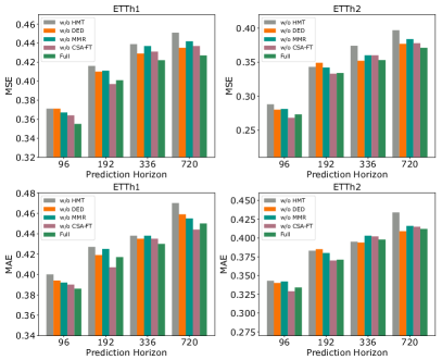
Figure 3: Component ablation of HiMTM: HMT, DED, MMR, and CSA-FT on ETTh1 and ETTh2.

In HiMTM, there are four key components: HMT, DED, MMR, and CSA-FT. We perform an ablation study on ETTh1 and ETTh2. The experimental results are shown in Figure 3, where ”w/o HMT” represents not employing HMT, ”w/o DED” represents not employing DED, ”w/o MMR” represents not employing MMR, and ”w/o CSA-FT” represents not employing CSA-FT. Since MMR and CSA-FT are closely related to HMT, we have to use fixed-scale masked reconstruction for pre-training and no cross-scale attention fine-tuning. From Figure 3 we can observe that the MSE and MAE increase significantly when any component is removed, which illustrates the effectiveness of each component.

4.4 Transfer Learning

We pre-trained on one dataset and fine-tuned it for another to verify the performance of HiMTM on the transfer learning tasks. We added two self-supervised learning methods Yue et al. (2022) and Woo et al. (2022) for comparison. The experimental results are shown in Table 2, where ETTh2 $\rightarrow$ ETTh1 denotes pre-training on ETTh2 and transfer to ETTh1. It can be found that HiMTM consistently achieves advanced performance compared to 8 mainstream self-supervised baselines.

Table 2: Complete results of HiMTM with 8 self-supervised learning methods on transfer learning tasks, where ETTh2 $\rightarrow$ ETTh1 denotes pre-training on ETTh2 and transfer to ETTh1. The best results are in bold.

Models		HiMTM		PatchTST*		SimMTM		Ti-MAE		TST		LaST		TF-C		CoST		TS2Vec
Metric		MSE	MAE	MSE	MAE	MSE	MAE	MSE	MAE	MSE	MAE	MSE	MAE	MSE	MAE	MSE	MAE	MSE	MAE
ETTh2 $\downarrow$ ETTh1	96	0.366	0.389	0.366	0.395	0.372	0.401	0.703	0.562	0.653	0.468	0.362	0.420	0.596	0.569	0.378	0.421	0.849	0.694
	192	0.405	0.412	0.406	0.422	0.414	0.425	0.715	0.567	0.658	0.502	0.426	0.478	0.614	0.621	0.424	0.451	0.909	0.738
	336	0.426	0.442	0.426	0.438	0.429	0.436	0.733	0.579	0.631	0.561	0.522	0.509	0.694	0.664	0.651	0.582	1.082	0.775
	720	0.447	0.465	0.444	0.461	0.446	0.458	0.762	0.622	0.638	0.608	0.460	0.478	0.635	0.683	0.883	0.701	0.934	0.769
	Avg	0.411	0.427	0.411	0.429	0.415	0.430	0.728	0.583	0.645	0.535	0.443	0.471	0.635	0.634	0.584	0.539	0.944	0.744
ETTm1 $\downarrow$ ETTh1	96	0.367	0.399	0.372	0.401	0.367	0.398	0.715	0.581	0.627	0.477	0.360	0.374	0.666	0.647	0.423	0.450	0.991	0.765
	192	0.397	0.410	0.404	0.419	0.396	0.421	0.729	0.587	0.628	0.500	0.381	0.371	0.672	0.653	0.641	0.578	0.829	0.699
	336	0.435	0.447	0.443	0.449	0.471	0.437	0.712	0.583	0.683	0.554	0.472	0.531	0.626	0.711	0.863	0.694	0.971	0.787
	720	0.452	0.467	0.470	0.472	0.454	0.463	0.747	0.627	0.642	0.600	0.490	0.488	0.835	0.797	1.071	0.805	1.037	0.820
	Avg	0.413	0.431	0.422	0.435	0.422	0.430	0.726	0.595	0.645	0.533	0.426	0.441	0.700	0.702	0.750	0.632	0.957	0.768
ETTm2 $\downarrow$ ETTh1	96	0.360	0.387	0.365	0.396	0.388	0.421	0.699	0.566	0.559	0.489	0.428	0.454	0.968	0.738	0.377	0.419	0.783	0.669
	192	0.404	0.419	0.407	0.423	0.419	0.423	0.722	0.573	0.600	0.579	0.427	0.497	1.080	0.801	0.422	0.450	0.828	0.691
	336	0.422	0.436	0.436	0.445	0.435	0.444	0.714	0.569	0.677	0.572	0.528	0.540	1.091	0.824	0.648	0.580	0.990	0.762
	720	0.453	0.471	0.478	0.477	0.468	0.474	0.760	0.611	0.694	0.664	0.527	0.537	1.226	0.893	0.880	0.699	0.985	0.783
	Avg	0.410	0.428	0.421	0.435	0.428	0.441	0.724	0.580	0.632	0.576	0.503	0.507	1.091	0.814	0.582	0.537	0.896	0.726
ETTh1 $\downarrow$ ETTm1	96	0.288	0.337	0.285	0.342	0.290	0.348	0.667	0.521	0.425	0.381	0.295	0.387	0.672	0.600	0.248	0.332	0.605	0.561
	192	0.344	0.367	0.329	0.372	0.327	0.372	0.561	0.479	0.495	0.478	0.335	0.379	0.721	0.639	0.336	0.391	0.615	0.561
	336	0.354	0.379	0.362	0.394	0.357	0.392	0.690	0.533	0.456	0.441	0.379	0.363	0.755	0.664	0.381	0.421	0.763	0.677
	720	0.402	0.415	0.406	0.417	0.409	0.423	0.744	0.583	0.554	0.477	0.403	0.431	0.837	0.705	0.469	0.482	0.805	0.664
	Avg	0.347	0.375	0.346	0.381	0.346	0.384	0.666	0.529	0.482	0.444	0.353	0.390	0.746	0.652	0.359	0.407	0.697	0.616
ETTh2 $\downarrow$ ETTm1	96	0.280	0.333	0.282	0.343	0.322	0.347	0.658	0.505	0.449	0.343	0.314	0.396	0.677	0.603	0.253	0.342	0.466	0.480
	192	0.355	0.365	0.333	0.370	0.332	0.372	0.594	0.511	0.477	0.407	0.587	0.545	0.718	0.638	0.367	0.392	0.557	0.532
	336	0.363	0.381	0.369	0.393	0.394	0.391	0.732	0.532	0.407	0.519	0.631	0.584	0.755	0.663	0.388	0.431	0.646	0.576
	720	0.397	0.414	0.417	0.423	0.411	0.424	0.768	0.592	0.557	0.523	0.368	0.429	0.848	0.712	0.498	0.488	0.752	0.638
	Avg	0.349	0.373	0.350	0.382	0.365	0.384	0.356	0.535	0.472	0.448	0.475	0.489	0.750	0.654	0.377	0.413	0.606	0.556
ETTm2 $\downarrow$ ETTm1	96	0.286	0.336	0.286	0.343	0.297	0.348	0.647	0.497	0.471	0.422	0.304	0.388	0.610	0.577	0.239	0.331	0.586	0.515
	192	0.331	0.363	0.333	0.370	0.332	0.370	0.597	0.508	0.495	0.442	0.429	0.494	0.725	0.657	0.339	0.371	0.624	0.562
	336	0.360	0.382	0.362	0.393	0.364	0.393	0.700	0.525	0.455	0.424	0.499	0.523	0.768	0.684	0.371	0.421	1.035	0.806
	720	0.405	0.411	0.417	0.423	0.410	0.421	0.786	0.596	0.498	0.532	0.422	0.450	0.927	0.759	0.467	0.481	0.780	0.669
	Avg	0.346	0.373	0.350	0.382	0.351	0.383	0.682	0.531	0.480	0.455	0.414	0.464	0.758	0.669	0.354	0.401	0.756	0.638

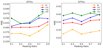
Figure 4: Forecasting performance with varying masking ratios $M=\{0.1,0.3,0.5,0.7,0.9\}$ for different prediction horizons.

Figure 5: Forecasting performance with the varying look-back window $L\in\{96,192,336,512,720\}$.

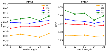
Figure 6: Forecasting performance with varying patch lengths $P=\{8,12,16,24,32\}$.

4.5 Masking Ratio

In this part, we study the impact of the masking ratio on prediction performance on ETTh1 and ETTh2. The experimental results are shown in Figure 4. We can find that the model performs worse when setting a lower masking ratio. The main reason is that reconstruction with a lower masking rate can be easily achieved by simple interpolation, so the feature extraction capabilities of the encoder cannot be fully stimulated. The model performs similarly poorly when using higher masking rates. The main reason is that fewer semantic units as input bring a huge challenge for reconstruction. In experiments, we found that a masking ratio of 50% brought higher prediction accuracy.

4.6 Varying Look-back Window

In this part, we verified the impact of the look-back window for prediction accuracy on ETTh1 and ETTh2. We report the change of MSE with the look-back window in Figure 5. It can be found that as the look-back window increases, the forecasting performance also improves. When the look-back window reaches 512, the prediction performance reaches the best. When the look-back window is set to 720, the prediction performance decreases. This shows that a too-long look-back window will bring redundant information and lead to performance degradation.

4.7 Varying Patch Length

This part studies the impact of patch length for HiMTM on ETTh1 and ETTh2. We fixed the look-back window to 512 and changed the length of patch $P=\{8,12,16,24,32\}$. The experimental results are shown in the Figure 6. We found that the MSE did not fluctuate significantly with changes in patch length. The main reason is that HiMTM selects patches of different lengths as semantic units at different hierarchies, so it can capture the temporal dependence of different scales well and show more stable performance on different datasets.

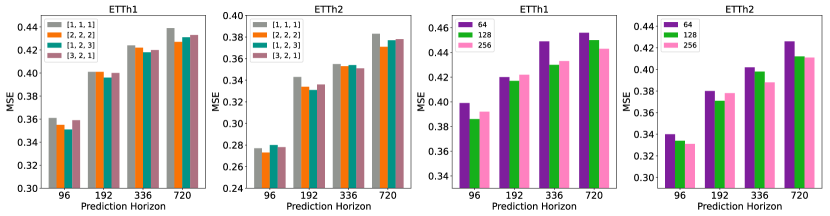
Figure 7: Forecasting performance with varying model parameters.

4.8 Varying Model Parameters

This part studies the impact of varying model parameters on the prediction accuracy of HiMTM on the ETTh1 and ETTh2. To this end, we set up two sets of experiments involving varying encoder depth and representation dimensions. For the encoder depth, we set $L=\{[1,1,1],[2,2,2],[1,2,3],[3,2,1]\}$. Each setting represents the number of Transformer layers at different hierarchies. The experimental results are shown in the left part of Figure 7. For the representation dimensions, we set $D=\{64,128,256\}$, and the experimental results are shown in the right part of Figure 7. Overall, HiMTM is robust to different model parameters.

4.9 Visualization

As shown in Figure 8, we visualize the prediction results of HiMTM and PatchTST with 96 horizons on the ETTh1, ETTh1, ETTm1, and ETTm2 datasets. The orange line represents the ground truth and the blue line represents the prediction results. It can be found that HiMTM can better fit seasons and trends compared to PatchTST*.

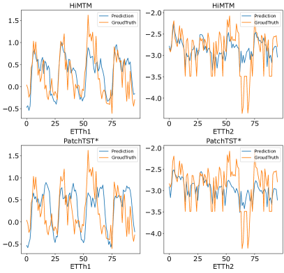
Figure 8: Prediction visualization of HiMTM and PatchTST* on ETTh1 and ETTh2 datasets.

5 Industrial Application

ENN Energy Holdings Co., Ltd. is the flagship industry of ENN Group and one of the largest clean energy distributors in China. It is committed to providing consumers with natural gas and other multi-category clean energy products, providing integrated energy and carbon solutions, and developing products and services around consumer needs. Over the past 30 years, we have accumulated a large amount of historical natural gas usage data from consumers in various domains. In this case study, we collected data from 42315 industrial consumers, 450 heating stations, and 2900 communities from 2017 to 2023 to train HiMTM. We selected 50 heating stations and 500 communities to verify its zero-shot learning capabilities in heating scenarios, which is crucial to ENN Group. Table 3 shows the experimental results of zero-shot forecasting of pre-trained HiMTM and PatchTST on ENN Natural Gas datasets. It can be found from the experimental results that HiMTM is significantly improved compared to PatchTST* in the Heating Station and Community.

Table 3: Complete results of HiMTM with PatchTST* for zero-shot learning tasks on ENN Natural Gas datasets.

Models		HiMTM		PatchTST*
Metric		MSE	MAE	MSE	MAE
Heating Station	7	0.202	0.262	0.225	0.291
	15	0.272	0.292	0.287	0.315
	30	0.344	0.350	0.377	0.369
	60	0.364	0.412	0.401	0.445
	Avg	0.295	0.329	0.322	0.355
Community	15	0.213	0.239	0.218	0.251
	30	0.227	0.258	0.234	0.266
	60	0.241	0.272	0.250	0.282
	120	0.261	0.293	0.270	0.321
	Avg	0.235	0.265	0.243	0.280

6 Conclusion

This paper presents HiMTM, a hierarchical multi-scale masked time series modeling for long-term forecasting. It contains four core modules, namely hierarchical multi-scale transformer(HMT), decoupled encoder-decoder(DED), multi-scale masked reconstruction(MMR), and cross-scale attention fine-tuning(CSA-FT). These components enable us to provide multi-scale feature extraction capabilities for masked time series modeling. Extensive experiments show that HiMTM surpasses previous self-supervised representation learning and end-to-end methods. This demonstrates the potential of self-supervised learning for time series forecasting. In the future, we will study HiMTM for various time series analysis tasks, including but not limited to forecasting, classification, anomaly detection, etc. In addition, we consider applying HiMTM to large-scale, multi-domain time series data sets to establish a general foundation model for time series analysis.

References

- Baevski et al. [2022] Alexei Baevski, Wei-Ning Hsu, Qiantong Xu, Arun Babu, Jiatao Gu, and Michael Auli. Data2vec: A general framework for self-supervised learning in speech, vision and language. In International Conference on Machine Learning, pages 1298–1312. PMLR, 2022.
- Benidis et al. [2022] Konstantinos Benidis, Syama Sundar Rangapuram, Valentin Flunkert, Yuyang Wang, Danielle Maddix, Caner Turkmen, Jan Gasthaus, Michael Bohlke-Schneider, David Salinas, Lorenzo Stella, et al. Deep learning for time series forecasting: Tutorial and literature survey. ACM Computing Surveys, 55(6):1–36, 2022.
- Chen et al. [2023a] Ling Chen, Donghui Chen, Zongjiang Shang, Binqing Wu, Cen Zheng, Bo Wen, and Wei Zhang. Multi-scale adaptive graph neural network for multivariate time series forecasting. IEEE Transactions on Knowledge and Data Engineering, 2023.
- Chen et al. [2023b] Xiaokang Chen, Mingyu Ding, Xiaodi Wang, Ying Xin, Shentong Mo, Yunhao Wang, Shumin Han, Ping Luo, Gang Zeng, and Jingdong Wang. Context autoencoder for self-supervised representation learning. International Journal of Computer Vision, pages 1–16, 2023.
- Chen et al. [2023c] Zonglei Chen, Minbo Ma, Tianrui Li, Hongjun Wang, and Chongshou Li. Long sequence time-series forecasting with deep learning: A survey. Information Fusion, 97:101819, 2023.
- Cheng et al. [2023] Mingyue Cheng, Qi Liu, Zhiding Liu, Hao Zhang, Rujiao Zhang, and Enhong Chen. Timemae: Self-supervised representations of time series with decoupled masked autoencoders. arXiv preprint arXiv:2303.00320, 2023.
- Cui et al. [2016] Zhicheng Cui, Wenlin Chen, and Yixin Chen. Multi-scale convolutional neural networks for time series classification. arXiv preprint arXiv:1603.06995, 2016.
- Dong et al. [2023] Jiaxiang Dong, Haixu Wu, Haoran Zhang, Li Zhang, Jianmin Wang, and Mingsheng Long. Simmtm: A simple pre-training framework for masked time-series modeling. arXiv preprint arXiv:2302.00861, 2023.
- Du et al. [2021] Yuntao Du, Jindong Wang, Wenjie Feng, Sinno Pan, Tao Qin, Renjun Xu, and Chongjun Wang. Adarnn: Adaptive learning and forecasting of time series. In Proceedings of the 30th ACM international conference on information & knowledge management, pages 402–411, 2021.
- Du et al. [2023] Dazhao Du, Bing Su, and Zhewei Wei. Preformer: predictive transformer with multi-scale segment-wise correlations for long-term time series forecasting. In ICASSP 2023-2023 IEEE International Conference on Acoustics, Speech and Signal Processing (ICASSP), pages 1–5. IEEE, 2023.
- Eldele et al. [2023] Emadeldeen Eldele, Mohamed Ragab, Zhenghua Chen, Min Wu, Chee-Keong Kwoh, and Xiaoli Li. Label-efficient time series representation learning: A review. arXiv preprint arXiv:2302.06433, 2023.
- Ericsson et al. [2022] Linus Ericsson, Henry Gouk, Chen Change Loy, and Timothy M Hospedales. Self-supervised representation learning: Introduction, advances, and challenges. IEEE Signal Processing Magazine, 39(3):42–62, 2022.
- Esling and Agon [2012] Philippe Esling and Carlos Agon. Time-series data mining. ACM Computing Surveys (CSUR), 45(1):1–34, 2012.
- Grill et al. [2020] Jean-Bastien Grill, Florian Strub, Florent Altché, Corentin Tallec, Pierre Richemond, Elena Buchatskaya, Carl Doersch, Bernardo Avila Pires, Zhaohan Guo, Mohammad Gheshlaghi Azar, et al. Bootstrap your own latent-a new approach to self-supervised learning. Advances in neural information processing systems, 33:21271–21284, 2020.
- He et al. [2020] Kaiming He, Haoqi Fan, Yuxin Wu, Saining Xie, and Ross Girshick. Momentum contrast for unsupervised visual representation learning. In Proceedings of the IEEE/CVF conference on computer vision and pattern recognition, pages 9729–9738, 2020.
- He et al. [2022] Kaiming He, Xinlei Chen, Saining Xie, Yanghao Li, Piotr Dollár, and Ross Girshick. Masked autoencoders are scalable vision learners. In Proceedings of the IEEE/CVF Conference on Computer Vision and Pattern Recognition, pages 16000–16009, 2022.
- Jin et al. [2023] Ming Jin, Qingsong Wen, Yuxuan Liang, Chaoli Zhang, Siqiao Xue, Xue Wang, James Zhang, Yi Wang, Haifeng Chen, Xiaoli Li, et al. Large models for time series and spatio-temporal data: A survey and outlook. arXiv preprint arXiv:2310.10196, 2023.
- Li et al. [2023a] Yiduo Li, Shiyi Qi, Zhe Li, Zhongwen Rao, Lujia Pan, and Zenglin Xu. Smartformer: Semi-autoregressive transformer with efficient integrated window attention for long time series forecasting. In Proceedings of the Thirty-Second International Joint Conference on Artificial Intelligence, pages 2169–2177, 2023.
- Li et al. [2023b] Zhe Li, Zhongwen Rao, Lujia Pan, Pengyun Wang, and Zenglin Xu. Ti-mae: Self-supervised masked time series autoencoders. arXiv preprint arXiv:2301.08871, 2023.
- Lim and Zohren [2021] Bryan Lim and Stefan Zohren. Time-series forecasting with deep learning: a survey. Philosophical Transactions of the Royal Society A, 379(2194):20200209, 2021.
- Liu et al. [2023] Ran Liu, Ellen L Zippi, Hadi Pouransari, Chris Sandino, Jingping Nie, Hanlin Goh, Erdrin Azemi, and Ali Moin. Frequency-aware masked autoencoders for multimodal pretraining on biosignals. arXiv preprint arXiv:2309.05927, 2023.
- Ma et al. [2023] Qianli Ma, Zhen Liu, Zhenjing Zheng, Ziyang Huang, Siying Zhu, Zhongzhong Yu, and James T Kwok. A survey on time-series pre-trained models. arXiv preprint arXiv:2305.10716, 2023.
- Nie et al. [2022] Yuqi Nie, Nam H Nguyen, Phanwadee Sinthong, and Jayant Kalagnanam. A time series is worth 64 words: Long-term forecasting with transformers. arXiv preprint arXiv:2211.14730, 2022.
- Pang et al. [2022] Yatian Pang, Wenxiao Wang, Francis EH Tay, Wei Liu, Yonghong Tian, and Li Yuan. Masked autoencoders for point cloud self-supervised learning. In European conference on computer vision, pages 604–621. Springer, 2022.
- Shabani et al. [2022] Amin Shabani, Amir Abdi, Lili Meng, and Tristan Sylvain. Scaleformer: iterative multi-scale refining transformers for time series forecasting. arXiv preprint arXiv:2206.04038, 2022.
- Shao et al. [2022] Zezhi Shao, Zhao Zhang, Fei Wang, and Yongjun Xu. Pre-training enhanced spatial-temporal graph neural network for multivariate time series forecasting. In Proceedings of the 28th ACM SIGKDD Conference on Knowledge Discovery and Data Mining, pages 1567–1577, 2022.
- Wang et al. [2022a] Huiqiang Wang, Jian Peng, Feihu Huang, Jince Wang, Junhui Chen, and Yifei Xiao. Micn: Multi-scale local and global context modeling for long-term series forecasting. In The Eleventh International Conference on Learning Representations, 2022.
- Wang et al. [2022b] Zhiyuan Wang, Xovee Xu, Weifeng Zhang, Goce Trajcevski, Ting Zhong, and Fan Zhou. Learning latent seasonal-trend representations for time series forecasting. Advances in Neural Information Processing Systems, 35:38775–38787, 2022.
- Wen et al. [2022] Qingsong Wen, Tian Zhou, Chaoli Zhang, Weiqi Chen, Ziqing Ma, Junchi Yan, and Liang Sun. Transformers in time series: A survey. arXiv preprint arXiv:2202.07125, 2022.
- Wen et al. [2023] Qingsong Wen, Tian Zhou, Chaoli Zhang, Weiqi Chen, Ziqing Ma, Junchi Yan, and Liang Sun. Transformers in time series: A survey. In International Joint Conference on Artificial Intelligence (IJCAI), 2023.
- Woo et al. [2022] Gerald Woo, Chenghao Liu, Doyen Sahoo, Akshat Kumar, and Steven Hoi. Cost: Contrastive learning of disentangled seasonal-trend representations for time series forecasting. arXiv preprint arXiv:2202.01575, 2022.
- Wu et al. [2021] Haixu Wu, Jiehui Xu, Jianmin Wang, and Mingsheng Long. Autoformer: Decomposition transformers with auto-correlation for long-term series forecasting. Advances in Neural Information Processing Systems, 34:22419–22430, 2021.
- Wu et al. [2022] Haixu Wu, Tengge Hu, Yong Liu, Hang Zhou, Jianmin Wang, and Mingsheng Long. Timesnet: Temporal 2d-variation modeling for general time series analysis. In The Eleventh International Conference on Learning Representations, 2022.
- Yue et al. [2022] Zhihan Yue, Yujing Wang, Juanyong Duan, Tianmeng Yang, Congrui Huang, Yunhai Tong, and Bixiong Xu. Ts2vec: Towards universal representation of time series. In Proceedings of the AAAI Conference on Artificial Intelligence, volume 36, pages 8980–8987, 2022.
- Zeng et al. [2023] Ailing Zeng, Muxi Chen, Lei Zhang, and Qiang Xu. Are transformers effective for time series forecasting? In Proceedings of the AAAI conference on artificial intelligence, volume 37, pages 11121–11128, 2023.
- Zerveas et al. [2021] George Zerveas, Srideepika Jayaraman, Dhaval Patel, Anuradha Bhamidipaty, and Carsten Eickhoff. A transformer-based framework for multivariate time series representation learning. In Proceedings of the 27th ACM SIGKDD Conference on Knowledge Discovery & Data Mining, pages 2114–2124, 2021.
- Zhang and Yan [2022] Yunhao Zhang and Junchi Yan. Crossformer: Transformer utilizing cross-dimension dependency for multivariate time series forecasting. In The Eleventh International Conference on Learning Representations, 2022.
- Zhang et al. [2022] Xiang Zhang, Ziyuan Zhao, Theodoros Tsiligkaridis, and Marinka Zitnik. Self-supervised contrastive pre-training for time series via time-frequency consistency. Advances in Neural Information Processing Systems, 35:3988–4003, 2022.
- Zhang et al. [2023a] Chaoning Zhang, Chenshuang Zhang, Junha Song, John Seon Keun Yi, and In So Kweon. A survey on masked autoencoder for visual self-supervised learning. In Proceedings of the Thirty-Second International Joint Conference on Artificial Intelligence, pages 6805–6813, 2023.
- Zhang et al. [2023b] Kexin Zhang, Qingsong Wen, Chaoli Zhang, Rongyao Cai, Ming Jin, Yong Liu, James Zhang, Yuxuan Liang, Guansong Pang, Dongjin Song, et al. Self-supervised learning for time series analysis: Taxonomy, progress, and prospects. arXiv preprint arXiv:2306.10125, 2023.
- Zhang et al. [2023c] Yitian Zhang, Liheng Ma, Soumyasundar Pal, Yingxue Zhang, and Mark Coates. Multi-resolution time-series transformer for long-term forecasting. arXiv preprint arXiv:2311.04147, 2023.
- Zheng et al. [2023] Xiaochen Zheng, Xingyu Chen, Manuel Schürch, Amina Mollaysa, Ahmed Allam, and Michael Krauthammer. Simts: Rethinking contrastive representation learning for time series forecasting. arXiv preprint arXiv:2303.18205, 2023.
- Zhou et al. [2022] Tian Zhou, Ziqing Ma, Qingsong Wen, Xue Wang, Liang Sun, and Rong Jin. Fedformer: Frequency enhanced decomposed transformer for long-term series forecasting. In International Conference on Machine Learning, pages 27268–27286. PMLR, 2022.