Can fallback accretion on magnetar model power the X-ray flares simultaneously observed with gamma-rays of Gamma-ray bursts?

Abstract

The prompt emission, X-ray plateau, and X-ray flares of Gamma-ray bursts (GRB) are thought to be from internal dissipation, and the magnetar as the central engine with propeller fallback accretion is proposed to interpret the observed phenomena of GRBs. In this paper, by systematically searching for X-ray emission observed by Swift/Xry Telescope, we find that seven robust GRBs include both X-ray flares and plateau emissions with measured redshift. More interestingly, the X-ray flares/bumps for those seven GRBs are simultaneously observed in the gamma-ray band. By adopting the propeller fallback accretion model to fit the observed data, it is found that the free parameters of two GRBs (140512A and 180329B) can be constrained very well, while in the other five cases, more or less, they are not all sufficiently constrained. On the other hand, this requires that the conversion efficiency of the propeller is to be two or three times higher than that of the spindown dipole radiation of the magnetar. If this is the case, it is contradictory to the expectation from the propeller model: namely, a dirtier ejecta should be less efficient in producing gamma-ray emissions. Our results hint that at least the magnetar central engine with propeller fallback accretion model cannot interpret very well both the GRB X-ray flares simultaneously observed in the gamma-ray band and the X-ray flares of GRBs with a high Lorentz factor.

1. Introduction

The majority of long-duration gamma-ray bursts (LGRBs) are thought to originate from the deaths of massive stars, excepting for several specific events, i.e., GRB 060614 (Gehrels et al., 2006), GRB 191019A (Levan et al., 2023), GRB 211211A (Rastinejad et al., 2022; Troja et al., 2022; Yang et al., 2022), and GRB 211227A (Lü et al., 2022), and the $``$collapsar$"$ model has been widely accepted as the standard paradigm for LGRBs (Woosley, 1993; MacFadyen & Woosley, 1999). A black hole or a rapidly spinning, strongly magnetized neutron star (called a millisecond magnetar) as the central engine of a GRB may be formed after collapse (Usov, 1992; Thompson, 1994; Dai & Lu, 1998; Popham et al., 1999; Wheeler et al., 2000; Zhang & Mészáros, 2001; Metzger et al., 2008; Lyons et al., 2010; Lei et al., 2013; Lü & Zhang, 2014; Liu et al., 2017). It successfully launches the relativistic outflow, to break out of the stellar envelope of the progenitor star, and produces prompt gamma-ray emission, which passes through the photosphere, internal shocks, or undergoes magnetic dissipation, becoming transparent (Meszaros & Rees, 1993; Piran et al., 1993; Rees & Meszaros, 1994; Zhang & Yan, 2011; Zhang, 2018). The broadband afterglow emission is attributed to synchrotron emission from the external shock when the outflow is decelerated by a circumburst medium (Mészáros & Rees, 1997; Sari et al., 1998; Zhang et al., 2016).

There is a small fraction of LGRBs in which the prompt emission shows two or more sub-bursts of emission in the light curves, with quiescent times of up to hundreds of seconds, detected by both Fermi/Gamma-ray Burst Monitor (GBM) and Swift/Burst Alert Telescope (BAT) (Koshut et al., 1995; Lazzati, 2005; Burlon et al., 2008; Bernardini et al., 2013; Hu et al., 2014; Lan et al., 2018). Lan et al. (2018) investigated the spectral and temporal properties of two sub-bursts of emission in the prompt emission, and they did not find any statistically significant correlation in the duration and peak energy ($E_{\rm p}$) of the two sub-bursts of emission. This suggests that those two or more sub-bursts of emission of GRB are likely to be from the same origin.

Thanks to Swift, a multiwavelength GRB mission (Gehrels et al., 2004) has led to great progress in understanding the nature of this phenomenon (review for Zhang 2007). Especially, the prompt slewing capability of the onboard X-ray Telescope (XRT; Burrows et al. 2004) has revealed the discovery of a canonical X-ray light curve following the prompt emission, which shows successively four power-law decay segments (i.e., an initial steep decay segment, a shallow decay segment, a normal decay segment, and a post-jet-break phase), with superimposed erratic flares (Nousek et al., 2006; O’Brien et al., 2006; Zhang et al., 2006). Moreover, a small fraction of GRBs show an internal plateau in the X-ray light curve (Liang et al., 2007; Troja et al., 2007; Lyons et al., 2010; Rowlinson et al., 2010, 2013; Lü & Zhang, 2014).

From the theoretical point of view, both the internal plateau and the X-ray flares are inconsistent with any external shock model, but must be attributed to the internal dissipation of a central engine wind. There are two forms of continuous energy injection into the external forward shock. One involves invoking a long-lasting central engine such as a spinning-down millisecond magnetar (Dai & Lu, 1998; Zhang & Mészáros, 2001). The other one involves a stratification of the ejecta Lorentz factor in an impulsively ejected fireball (Rees & Mészáros, 1998; Sari & Mészáros, 2000; Uhm et al., 2012). The widely discussed model for dealing with the energy injection process involves assuming a millisecond magnetar as the central engine (Zhang & Mészáros, 2001; Toma et al., 2007; Troja et al., 2007; Lü & Zhang, 2014; Rea et al., 2015; Stratta et al., 2018; Fraija et al., 2021). Within the scenario of a magnetar central engine, the energy injection to explain the plateau (or shallow decay) phase is from the dipole radiation of the magnetar spindown. This has previously been studied for LGRBs (e.g., Lyons et al. 2010; Dall’Osso et al. 2011; Lü & Zhang 2014), short GRBs (e.g., Rowlinson et al. 2013; Lü et al. 2015, 2017), as well as the extended emission of short GRBs (e.g., Gompertz et al. 2013). These works assumed a constant rate of spindown and therefore a constant level of dipole luminosity.

Another component, a flare/bump in the X-ray emission, is also of an important clue to understanding the physical process in the framework of the magnetar central engine. This has been discovered in a good fraction of GRBs (Barthelmy et al., 2005; Chincarini et al., 2007; Falcone et al., 2007; Cusumano et al., 2010; Margutti et al., 2010). In most cases, flares/bumps are superposed on either the steep decay phase or the shallow decay phase (Nousek et al., 2006; Zhang et al., 2006). Peng et al. (2014) found that a good fraction of GRB X-ray flares, which were observed simultaneously by both BAT and XRT on board the Swift mission, obeyed the same power-law spectral fit. By studying the properties of both temporal and spectral behaviors, this suggests that the X-ray flares are produced by late central engine activities, and may share the same physical origin as the prompt emission of GRBs (Burrows et al., 2005; Yi et al., 2016). If this is the case, a small fraction of the GRB X-ray flares at least can be used to constrain the Lorentz factors, which range from a few tens to hundreds (Jin et al., 2010; Yi et al., 2015). On the other hand, several models have also been invoked to interpret the X-ray flares, such as the tail of prompt emission with a high-latitude curvature effect (Liang et al., 2006), delayed magnetic dissipation activity as the ejecta decelerates (Giannios, 2006), and anisotropic emission in the blast wave comoving frame (Beloborodov et al., 2011). Moreover, the magnetar central engine with the delayed onset of a propeller regime, which accelerates local material via magnetocentrifugal slinging, has also been proposed to explain the X-ray flares in GRBs (Gibson et al., 2017, 2018). This model has also been invoked to account for supernova explosions (Piro & Ott, 2011) and X-ray plateaus for short GRBs (Gompertz et al., 2014). However, the main issue of the propeller mechanism for explaining the prompt emission of GRBs is baryon loading. The propeller mechanism expels a lot of unaccreted material from the system, and the outflow must be very dirty and nonrelativistic if the material is expelled in the funnel region. This means that no matter how large the power is, it cannot power a GRB itself.

One interesting question is whether the propeller mechanism with fallback accretion on the millisecond magnetar model can indeed interpret an X-ray light curve of a GRB that is composed of both plateau emission and an X-ray flare/bump. In this paper, by systematically searching for X-ray emission observed by Swift/XRT, we find X-ray light curves of seven GRBs composed of plateau emission and X-ray flares with measured redshift. The basic propeller with fallback accretion model of the magnetar central engine is shown in Section 2. In Section 3, we present the criteria for the sample selection, and the fitting results for those seven GRBs with the propeller model, by adopting the method of Markov Chain Monte Carlo (MCMC, Mackay 2003) are reported in Section 4. Finally, we summarize our discussion and conclusion in Section 5. Throughout the paper, a concordance cosmology with the parameters $H_{0}=71~{}\rm km~{}s^{-1}~{}Mpc^{-1}$, $\Omega_{M}=0.30$, and $\Omega_{\Lambda}=0.70$ is adopted.

2. The magnetar propeller with fallback accretion model

Previously, the propeller with fallback accretion model of a magnetar central engine was invoked to explain the short GRB with extended emission (Gompertz et al., 2014; Gibson et al., 2017; Lan et al., 2020), X-ray plateau emission and X-ray flares in long-duration GRBs (Gibson et al., 2018), as well as some stripped-envelope Supernovae (Lin et al., 2021). In this section, we will briefly introduce the model of magnetar propeller with fallback accretion.

The propeller regime is basically defined by the relationship between the Alfvén radius ($r_{\rm m}$) and the co-rotation radius ($r_{\rm c}$). Generally speaking, when $r_{\rm c}<r_{\rm m}$, the materials already within $r_{\rm c}$ accrete to the surface of the magnetar, while the materials within the range of $r_{\rm c}$ and $r_{\rm m}$ are propelled away at $r_{\rm m}$. If the power of propeller is not strong enough for materials, it cannot reach the potential well. Then, the materials will return to the disc without any emission to be detected (called “propeller regime” Illarionov & Sunyaev 1975). Based on the paper of Gibson et al. (2017), $r_{\rm m}$ and $r_{\rm c}$ can be defined as follows,

$$r_{\mathrm{m}}=\mu^{4/7}(GM)^{-1/7}\left(\dfrac{3M_{\mathrm{d}}}{t_{\nu}}\right)^{-2/7},$$ (1)

$$r_{\mathrm{c}}=(GM/\omega^{2})^{1/3},$$ (2)

where $G$ is the gravitational constant, $\mu=B_{\rm p}R^{3}$ is the magnetic dipole moment, $B_{\rm p}$ is the surface magnetic field, $M$ and $R$ are the mass and radius of magnetar, respectively. $t_{\nu}=R_{\rm d}/\alpha c_{\rm s}$ is the viscous time-scale, $\alpha$ and $c_{\rm s}$ are the viscosity prescription and the speed of sound in the disc, respectively. $\omega$ is the angular frequency of the magnetar, $M_{\rm d}$ and $R_{\rm d}$ are the mass and radius of disc, respectively. In our calculations, we adopt $\alpha=0.1$ and $c_{\rm s}=10^{7}\mathrm{cm}\cdot\mathrm{s}^{-1}$ (Gompertz et al., 2014).

At the Alfvén radius $r_{\rm m}$, the effect of materials from the accretion is smaller than that of magnetic field of magnetar. While, at the co-rotation radius $r_{\rm c}$, the rotation rate of matter in the disc is the same as that of the stellar surface. Since $r_{\rm m}$ and $r_{\rm c}$ depend on the disc mass and the frequency of the magnetar, respectively. The evolution of disc mass and frequency with time can be expressed as follows (Gibson et al., 2017),

$$\dot{M}_{\mathrm{d}}=\dot{M}_{\mathrm{fb}}-\dot{M}_{\mathrm{prop}}-\dot{M}_{\mathrm{acc}},$$ (3)

$$\dot{\omega}=\frac{N_{\mathrm{acc}}+N_{\mathrm{dip}}}{I}.$$ (4)

Here, $\dot{M}_{\mathrm{fb}}$ is the fallback mass changed with time, $\dot{M}_{\mathrm{prop}}$ and $\dot{M}_{\mathrm{acc}}$ are the mass lost via the propeller mechanism and the accretion to the magnetar, respectively. $N_{\mathrm{acc}}$ and $N_{\mathrm{dip}}$ are the accretion and dipole torques acting on the magnetar, respectively. $I=0.35MR^{2}$ is the magnetar moment of inertia.

Based on the description of Gibson et al. (2017), $\dot{M}_{\mathrm{fb}}$, $\dot{M}_{\mathrm{prop}}$, and $\dot{M}_{\mathrm{acc}}$ can be defined as follows,

$$\dot{M}_{\rm{fb}}=\frac{M_{\rm{fb}}}{t_{\rm{fb}}}\left(\dfrac{t+t_{\rm{fb}}}{t_{\rm{fb}}}\right)^{-5/3},$$ (5)

$$\dot{M}_{\rm{prop}}=\eta\left(\dfrac{M_{\rm{d}}}{t_{\nu}}\right),$$ (6)

$$\dot{M}_{\rm{acc}}=(1-\eta)\left(\dfrac{M_{\rm{d}}}{t_{\nu}}\right),$$ (7)

where $M_{\rm{fb}}=\delta M_{\rm d,0}$ is the available fallback mass, $M_{\rm d,0}$ is the initial mass of disc, and $\delta$ is the ratio between fallback mass and initial disc mass. $t_{\rm{fb}}=\epsilon t_{\nu}$ is the fallback time-scale, and $\epsilon$ is the ratio between fallback time-scale and viscous time-scale. $\eta=\dfrac{1}{2}(1+\tanh[n(\Omega-1)])$ is the efficiency of the propeller mechanism, and it related to the ”fastness parameter” $\Omega=\omega/(GM/r_{\mathrm{m}}^{3})^{1/2}=(r_{\mathrm{m}}/r_{\mathrm{c}})^{3/2}$. In this work, we adopt $n=1$ to do the calculations.

For the dipole torque, we adopt the classical solution as given by (Shapiro & Teukolsky, 1983) and (Piro & Ott, 2011),

$$N_{\text{dip}}=-\dfrac{\mu^{2}\omega^{3}}{6c^{3}}.$$ (8)

Moreover, $N_{\mathrm{acc}}$ has two forms that depend on the relationship between $r_{\rm m}$ and $R$. It reads as

$$N_{\mathrm{acc}}=(GMr_{\mathrm{m}})^{1/2}(\dot{M}_{\mathrm{acc}}-\dot{M}_{\mathrm{prop}}),~{}r_{\rm m}>R$$ (9)

$$N_{\mathrm{acc}}=(GMR)^{1/2}(\dot{M}_{\mathrm{acc}}-\dot{M}_{\mathrm{prop}}),~{}r_{\rm m}<R$$ (10)

Then, do the integration of equations 3 and 4, one can estimate the components of propelled luminosity and dipole luminosity,

$$L_{\text{prop}}=\eta_{\text{prop}}\left[-\omega N_{\text{acc}}-\left(\eta\dfrac{GMM_{\text{d}}}{r_{\text{m}}t_{\nu}}\right)\right],$$ (11)

$$L_{\mathrm{dip}}=\eta_{\mathrm{dip}}\dfrac{\mu^{2}\omega^{4}}{6c^{3}}.$$ (12)

Here, $\eta_{\text{prop}}$ and $\eta_{\text{dip}}$ are the conversion efficiencies of propeller and dipole energy-luminosity, respectively. The total luminosity is therefore defined as follows,

$$L_{\mathrm{tot}}=(1/f_{\mathrm{B}})(L_{\mathrm{dip}}+L_{\mathrm{prop}}),$$ (13)

where $1/f_{\rm B}$ is the fraction of the stellar sphere that is emitting, and it is related to the half-opening angle of the jet ($\theta_{j}$). One has $f_{\mathrm{B}}=1-\operatorname{cos}\left(\theta_{\mathrm{j}}\right)$ (Rhoads, 1999; Sari et al., 1999).

By given some typical parameters of magnetar propeller with fallback accretion model, such as $R=10^{6}~{}\rm cm$, $M=1.4~{}M_{\odot}$, $B_{\rm p}=10^{15}~{}\rm G$, $P_{0}=10^{-3}~{}\rm s$, $M_{\rm d,0}=10^{-3}M_{\odot}$, $R_{\rm d}=10^{7}~{}\rm cm$, $\epsilon=0.1$, $\delta=10^{-4}$, $\eta_{\rm prop}=0.8$, $\eta_{\rm dip}=0.1$, and $1/f_{B}=10^{1.7}$, one can plot the picture of luminosity as function of time for both propeller and dipole radiations (see Figure 1).

3. Sample Selection and Data Reduction

The XRT data is downloaded from the Swift data archive and the UK Swift Science Data Center (Evans et al., 2007, 2009). Our entire sample includes more than 1718 GRBs observed by Swift/XRT between January 2005 and June 2023. The magnetar signature typically exhibits a shallow decay phase (or plateau) followed by a normal decay in X-ray emission when it is spinning down, and the delayed onset of a propeller regime that accelerates local material via magneto-centrifugal slinging can produce the X-ray flares. We only focus on the long-duration GRBs with both flare/bump and plateau emissions observed in X-ray afterglow, and 154 GRBs are too faint to be detected in the X-ray band, or do not have enough photons to extract a reasonable X-ray light curve. Then, we select the GRBs whose X-ray emission exhibits the feature of plateau followed by a normal decay, and adopt a smooth broken power-law function to fit (Liang et al., 2007),

$$F_{1}(t)=F_{01}\left[\left(\frac{t}{t_{p}}\right)^{\omega\alpha_{1}}+\left(\frac{t}{t_{p}}\right)^{\omega\alpha_{2}}\right]^{-1/\omega},$$ (14)

where fixed $\omega=3$ represents the sharpness of the peak and $t_{p}$, $\alpha_{1}$, and $\alpha_{2}$ are the peak time, and decay slope of plateau and normal decay phase, respectively.

Within the above scenario, three criteria are adopted for our sample selection. (i) We focus on those long-duration GRBs that show such a transition from shallow decay to normal decay in the X-ray light curves, but require that the decay slope of the normal decay segment following the plateau phase should be in the range of $-1$ to $-2$ (Lü et al., 2018); (ii) It must include the X-ray flare/bump in the X-ray light curve; (iii) In order to estimate the intrinsic luminosity of the plateau emission, the redshift needs to be measured. By adopting the criteria for our sample selection, only seven robust cases identified to satisfy the above three criteria. The X-ray light curves are shown in Figure 3 (also see Table 1 for a summarized).

More interestingly, it is found that the X-ray flare/bump for those seven GRBs is simultaneously observed by Swift/BAT in $\gamma-$ray band by searching in GCN Circulars Archive case by case. So we downloaded the Swift/BAT data of the seven GRBs from the NASA Archive, and extracted the light curves with the standard Swift scientific tools. Based on the methods from Hu et al. (2014) for Swift/BAT, we employed the Bayesian Block (BBs; Scargle 1998) algorithm to search for possible signals and identify the light curves. In order to search for a low-significance signal before and after the duration, the extracted BAT light curves usually cover 300 s before the BAT triggers and after duration of the GRBs. More details, please refer to the paper on data analysis with the Bayesian Block algorithm (Hu et al., 2014). Phenomenally, we find that the prompt emission in $\gamma-$ray band of the seven GRBs are composed of two sub-bursts with the quiescent time. The light curves of the two sub-bursts exhibit different behavior for our sample, e.g., a softer sub-burst prior to (3 out of 7) or following (4 out of 7) the stronger sub-burst of prompt emission. The light curves of both prompt emission and X-ray flares for those seven GRBs are shown in Figure 2.

4. Fitting results with magnetar propeller-fallback-accretion model

One motivation is to test whether magnetar propeller-fallback-accretion model can be invoked to interpret the GRBs that we selected sample above. In order to find out the best fit parameters of magnetar propeller-fallback-accretion model, we adopt the MCMC simulation package (Foreman-Mackey et al., 2013) to fit the X-ray flare/bump and X-ray plateau in the afterglow. There are nine free parameters (i.e., $B_{\rm p}$, $P_{\rm 0}$, $M_{\rm d,0}$, $R_{\rm d}$, $\epsilon$, $\delta$, $\eta_{\rm dip}$, $\eta_{\rm prop}$, and $1/f_{\rm B}$) by invoking the propeller and dipole radiations of magnetar. The MCMC is one of the very popular methods in the field of high energy astronomy, and it is very effective in constraining the free parameters which are in degeneracy between each other. More details can refer to Gibson et al. (2017, 2018).

Initially, we set the range of those parameters as following, $B_{\rm p}\sim(10^{-3}-10)\times 10^{15}$ G, $P_{0}\sim(0.5-100)\times 10^{-3}$ s, $M_{\rm d,0}\sim(10^{-3}-10^{2})M_{\odot}$, $R_{\rm d}\sim(50-2000)\times 10^{5}$ cm, $\epsilon\sim(10^{-1}-10^{3})$, $\delta\sim(10^{-5}-50)$, $\eta_{\rm dip}\sim(1-100)\%$, $\eta_{\rm prop}\sim(1-100)\%$, $1/f_{B}\sim(1-600)$. Then, we adopt MCMC method to fit the X-ray light curve by invoking the propeller-fallback-accretion model and spin-down dipole radiation of magnetar.

Figure 3 shows the MCMC fitting results by using the propeller-fallback-accretion model and spin-down dipole radiation of magnetar for the seven GRBs. We find that the free parameters of GRBs 140512A and 180329B can be constrained very well, such as $B_{\rm p}$ and $P_{0}$, which are within a range of several times $10^{15}$ G and tens of milliseconds, respectively. The derived parameters of $B_{\rm p}$, $P_{0}$, and $M_{\rm d,0}$ fall into the reasonable range, and they are consistent with the results from Lü & Zhang (2014) and Gibson et al. (2018). However, the free parameters of the other five cases are, more or less, not all constrained well enough, especially, the main free parameters of propeller-fallback-accretion model, such as $B_{\rm p}$, $P_{0}$, and $M_{\rm d,0}$. The two-dimensional histograms and parameter constraints of model fit by invoking MCMC method for our sample are shown in Figure 4, and the values of parameter constraints are reported in Table 1. On the other hand, based on the fitting results, we find that the required conversion efficiency of propeller is two or three times (or even large) higher than that of spin-down dipole radiation of magnetar (see Figure 5 and Table 1). Based on the results from Lan et al. (2018) for Fermi/GBM and Peng et al. (2014) for Swift/BAT, it suggests that those two sub-bursts emission of GRB, together with the observed simultaneous X-ray flare/bump, are likely to share the same physical origin. However, the higher efficiency for the propeller phase in our fits is contradictory to the expectation from the propeller model, namely, a dirtier ejecta should be less efficient in producing $\gamma-$ray emissions. It means that at least the magnetar propeller-fallback-accretion model cannot interpret very well to the GRB X-ray flares that are simultaneously observed in $\gamma-$ray band, even though it can be invoked to interpret the X-ray plateaus for short GRBs (Gompertz et al., 2014) and supernova explosion (Piro & Ott, 2011).

5. Conclusion and Discussion

The prompt emission, X-ray plateau, and X-ray flares of GRBs are thought to be from internal dissipation (Zhang, 2011). The magnetar as the central engine of GRB has been proposed to interpret the observed X-ray flares and plateau emission (Gompertz et al., 2014; Gibson et al., 2017). By systematically searching for X-ray emission observed by Swift/XRT, we find that seven robust GRBs include both X-ray flares and plateau emissions with redshift measured. More interestingly, it is found that the X-ray flare/bump for those seven GRBs is simultaneously observed by Swift/BAT in $\gamma-$ray band. The prompt emission in $\gamma-$ray band of the seven GRBs is composed of two sub-bursts with the quiescent time. Especially, the second sub-burst emission in the prompt emission is observed simultaneously with X-ray flare.

Then, by adopting the MCMC method, we invoke the propeller-fallback-accretion model and spin-down dipole radiation of magnetar central to fit the X-ray data of plateau emissions and flares for our sample. It is found that the free parameters of two GRBs (GRBs 140512A and 180329B) can be constrained very well, such as $B_{\rm p}$ and $P_{0}$ are range of several times $10^{15}$ G and tens of milliseconds, respectively. However, the free parameters of the other five cases, more or less, are not all constrained well enough, especially, the main free parameters of propeller-fallback-accretion model, such as $B_{\rm p}$, $P_{0}$, and $M_{\rm d,0}$. On the other hand, it requires that the conversion efficiency of propeller is two or three times higher than that of spin-down dipole radiation of magnetars. If this is the case, the higher efficiency for the propeller phase in our fits is contradictory to the expectation from the propeller model, namely, a dirtier ejecta should be less efficient in producing $\gamma-$ray emissions. Our results suggest that at least the magnetar propeller-fallback-accretion model cannot interpret very well to the GRB X-ray flares that are simultaneously observed in $\gamma-$ray.

We believe that the magnetar propeller-fallback-accretion model can interpret very well the X-ray plateau emissions of some GRBs. However, this model exists significant challenges and flaws for the baryon loading issue when it is related to $\gamma-$ray emission and high relativistic outflow. From the observational point of view, the X-ray flares are observed in a good fraction of GRB afterglow, and the constrained bulk Lorentz factor (or just upper limit) of the X-ray flare outflows ranges from a few tens to hundreds (Jin et al., 2010; Yi et al., 2015). It means that the dirty of baryon loading issue still exists if we invoke the magnetar propeller-fallback-accretion model to interpret the X-ray flares with a highly Lorentz factor. Furthermore, several physical models without magnetar central engine are invoked to interpret the observed X-ray flare, plateau emission, as well as two sub-bursts $\gamma-$ray emission, such as late central engine reactivity (Burrows et al., 2005; Fan & Wei, 2005; Dai et al., 2006), the relativistic jet and cocoon emissions (Ramirez-Ruiz et al., 2002; Lazzati & Begelman, 2010; Nakar & Piran, 2017), two steps in the collapse of the progenitor star (Lipunova et al., 2009), the collapse of a rapidly rotating stellar core leading to fragmentation (King et al., 2005), fragmentation in the accretion disc (Perna et al., 2006), the magnetic barrier around the accretor (Proga & Zhang, 2006), the gravitational lensing (Paynter et al., 2021; Yang et al., 2021; Lin et al., 2022), and jet precession model (Gao et al., 2023). However, more or less, each model above cannot fully interpret all properties of observations for two sub-bursts emission of GRB from light curve, spectrum, as well as the quiescent time.

Table 1The values of derived parameters from the MCMC for our sample.

GRB	$B_{\rm p}$ $(10^{15}\cdot\rm G)$	$P_{0}$ $\rm(ms)$	$M_{\rm d,0}$ $(10^{-2}\cdot M_{\odot})$	$R_{\rm d}$ $\rm(km)$	$\epsilon$	$\delta$ $10^{-4}$	$\eta_{\rm prop}$	$\eta_{\rm dip}$	$1/f_{B}$	$z$
140512A	$2.28^{+0.01}_{-0.01}$	$69.85^{+1.51}_{-0.82}$	$8.13^{+0.04}_{-0.04}$	$148.95^{+0.14}_{-0.12}$	$19.72^{+0.23}_{-0.23}$	$73.62^{+0.34}_{-0.34}$	$0.56^{+0.01}_{-0.01}$	$0.23^{+0.01}_{-0.01}$	$7.93^{+0.13}_{-0.14}$	$0.725^{(a)}$
180329B	$6.30^{+0.01}_{-0.01}$	$29.93^{+0.23}_{-0.24}$	$0.44^{+0.01}_{-0.01}$	$116.53^{+0.10}_{-0.10}$	$0.28^{+0.02}_{-0.02}$	$2.32^{+0.12}_{-0.11}$	$0.24^{+0.01}_{-0.01}$	$0.08^{+0.01}_{-0.01}$	$29.04^{+1.30}_{-1.05}$	$1.998^{(b)}$
060526	$9.99^{+0.01}_{-0.01}$	$9.02^{+0.57}_{-0.43}$	$9.98^{+0.01}_{-0.03}$	$144.84^{+0.15}_{-0.12}$	$136.14^{+9.06}_{-22.64}$	$6.08^{+0.67}_{-0.78}$	$0.74^{+0.15}_{-0.10}$	$0.12^{+0.02}_{-0.02}$	$88.51^{+15.00}_{-14.38}$	$3.21^{(c)}$
061602	$1.278^{+0.07}_{-0.09}$	$7.98^{+1.40}_{-1.94}$	$9.56^{+0.32}_{-0.57}$	$81.27^{+1.15}_{-0.94}$	$0.20^{+0.24}_{-0.08}$	$37.75^{+16.19}_{-15.16}$	$0.78^{+0.15}_{-0.21}$	$0.06^{+0.01}_{-0.02}$	$10.47^{+3.75}_{-1.78}$	$2.253^{(d)}$
100906A	$4.00^{+0.18}_{-0.26}$	$9.32^{+0.43}_{-0.83}$	$9.75^{+0.18}_{-0.33}$	$90.96^{+0.39}_{-0.82}$	$161.43^{+15.16}_{-20.50}$	$29.64^{+4.70}_{-6.68}$	$0.79^{+0.13}_{-0.14}$	$0.02^{+0.01}_{-0.01}$	$16.25^{+3.46}_{-2.45}$	$1.727^{(e)}$
130609B	$5.75^{+0.10}_{-0.09}$	$1.44^{+0.03}_{-0.04}$	$9.84^{+0.11}_{-0.22}$	$236.09^{+2.89}_{-1.68}$	$57.94^{+2.31}_{-2.22}$	$130.01^{+4.87}_{-4.70}$	$0.55^{+0.15}_{-0.08}$	$0.28^{+0.08}_{-0.05}$	$55.46^{+12.45}_{-12.40}$	$1.3^{(f)}$
180325A	$3.29^{+0.09}_{-0.07}$	$9.68^{+0.21}_{-0.45}$	$9.77^{+0.15}_{-0.36}$	$65.67^{+1.37}_{-0.95}$	$109.14^{+6.46}_{-6.10}$	$883.07^{+28.93}_{-35.85}$	$0.72^{+0.17}_{-0.16}$	$0.08^{+0.14}_{-0.06}$	$6.35^{+1.94}_{-1.10}$	$2.25^{(g)}$

• References of redshift measured: (a) de Ugarte Postigo et al. (2014); (b) Izzo et al. (2018); (c) Berger & Gladders (2006); (d) Perley et al. (2016); (e) Tanvir et al. (2010); (f) Ruffini et al. (2013); (g) Heintz et al. (2018).

Figure 1.— X-ray light curve generated by propeller model with fallback accretion (blue dash-dotted line) and dipole radiation of spin-down (green dashed line) of magnetar central engine. The black solid line is the sum of propeller and dipole radiation of spin-down.

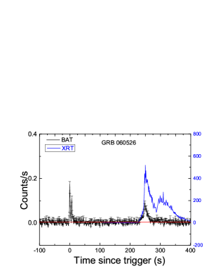
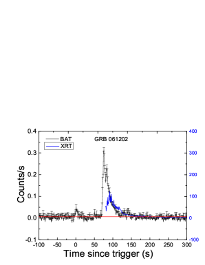
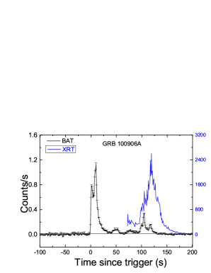
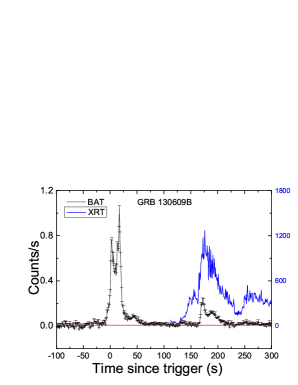
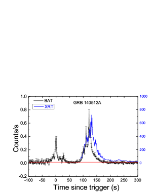
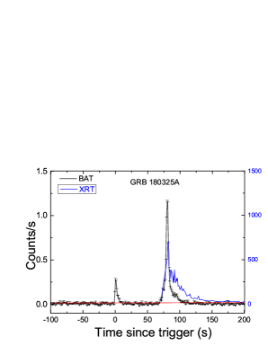
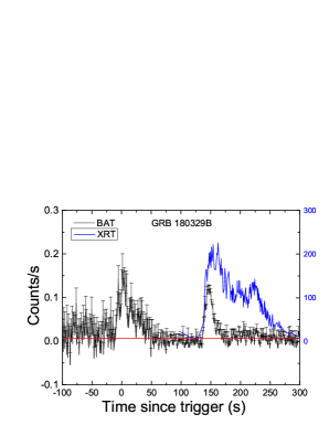
Figure 2.— BAT lightcurves (black) of prompt emission and X-ray flares (blue) for our sample. The solid red line is the background of prompt emission.

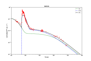
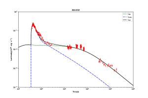
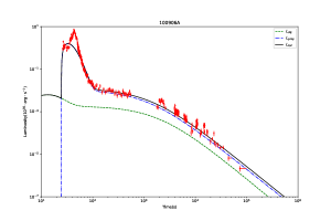
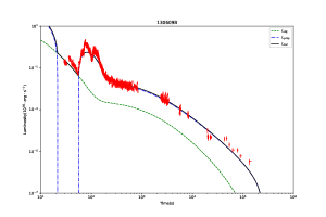
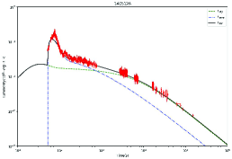
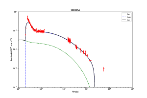
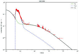
Figure 3.— X-ray light curves of GRBs for our sample (red points), as well as the fits by magnetar propeller model with fallback accretion (red dash-dotted line) and magnetar spin-down (blue dashed line). The black solid line is the total luminosity of propeller and spin-down.

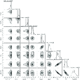
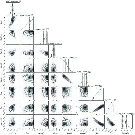
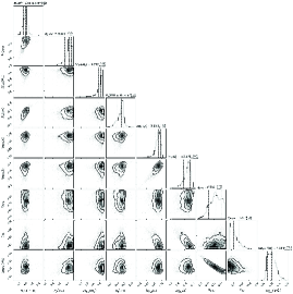
Figure 4.— 2D histograms and parameter constraints of model fit for our sample. The 1D histograms show the distribution for each parameter. The dashed lines indicate the median and $\pm 2\sigma$ uncertainty of the values.

Fig. 4— continued.

Figure 5.— Efficiency correlation between propeller and dipole radiation. The dotted line corresponds to $\eta_{\rm prop}=\eta_{\rm dip}$.

References

- Barthelmy et al. (2005) Barthelmy, S. D., Chincarini, G., Burrows, D. N., et al. 2005, Nature, 438, 994. doi:10.1038/nature04392
- Beloborodov et al. (2011) Beloborodov, A. M., Daigne, F., Mochkovitch, R., et al. 2011, MNRAS, 410, 2422. doi:10.1111/j.1365-2966.2010.17616.x
- Bernardini et al. (2013) Bernardini, M. G., Campana, S., Ghisellini, G., et al. 2013, ApJ, 775, 67. doi:10.1088/0004-637X/775/1/67
- Berger & Gladders (2006) Berger, E. & Gladders, M. 2006, GRB Coordinates Network, Circular Service, No. 5170, 1
- Burlon et al. (2008) Burlon, D., Ghirlanda, G., Ghisellini, G., et al. 2008, ApJ, 685, L19. doi:10.1086/592350
- Burrows et al. (2005) Burrows, D. N., Romano, P., Falcone, A., et al. 2005, Science, 309, 1833. doi:10.1126/science.1116168
- Burrows et al. (2004) Burrows, D. N., Hill, J. E., Nousek, J. A., et al. 2004, Proc. SPIE, 5165, 201. doi:10.1117/12.504868
- Chincarini et al. (2007) Chincarini, G., Moretti, A., Romano, P., et al. 2007, ApJ, 671, 1903. doi:10.1086/521591
- Cusumano et al. (2010) Cusumano, G., La Parola, V., Segreto, A., et al. 2010, A&A, 524, A64. doi:10.1051/0004-6361/201015249
- Dai & Lu (1998) Dai, Z. G. & Lu, T. 1998, Phys. Rev. Lett., 81, 4301. doi:10.1103/PhysRevLett.81.4301
- Dai et al. (2006) Dai, Z. G., Wang, X. Y., Wu, X. F., et al. 2006, Science, 311, 1127. doi:10.1126/science.1123606
- Dall’Osso et al. (2011) Dall’Osso, S., Stratta, G., Guetta, D., et al. 2011, A&A, 526, A121. doi:10.1051/0004-6361/201014168
- de Ugarte Postigo et al. (2014) de Ugarte Postigo, A., Gorosabel, J., Xu, D., et al. 2014, GRB Coordinates Network, Circular Service, No. 16310, 1
- Evans et al. (2009) Evans, P. A., Beardmore, A. P., Page, K. L., et al. 2009, MNRAS, 397, 1177. doi:10.1111/j.1365-2966.2009.14913.x
- Evans et al. (2007) Evans, P. A., Beardmore, A. P., Page, K. L., et al. 2007, A&A, 469, 379. doi:10.1051/0004-6361:20077530
- Falcone et al. (2007) Falcone, A. D., Morris, D., Racusin, J., et al. 2007, ApJ, 671, 1921. doi:10.1086/523296
- Fan & Wei (2005) Fan, Y. Z. & Wei, D. M. 2005, MNRAS, 364, L42. doi:10.1111/j.1745-3933.2005.00102.x
- Foreman-Mackey et al. (2013) Foreman-Mackey, D., Hogg, D. W., Lang, D., et al. 2013, PASP, 125, 306. doi:10.1086/670067
- Fraija et al. (2021) Fraija, N., Veres, P., Beniamini, P., et al. 2021, ApJ, 918, 12. doi:10.3847/1538-4357/ac0aed
- Gao et al. (2023) Gao, H., Li, A., Lei, W.-H., et al. 2023, ApJ, 945, 17. doi:10.3847/1538-4357/acba0d
- Gehrels et al. (2006) Gehrels, N., Norris, J. P., Barthelmy, S. D., et al. 2006, Nature, 444, 1044. doi:10.1038/nature05376
- Gehrels et al. (2004) Gehrels, N., Chincarini, G., Giommi, P., et al. 2004, ApJ, 611, 1005. doi:10.1086/422091
- Giannios (2006) Giannios, D. 2006, A&A, 455, L5. doi:10.1051/0004-6361:20065578
- Gibson et al. (2018) Gibson, S. L., Wynn, G. A., Gompertz, B. P., et al. 2018, MNRAS, 478, 4323. doi:10.1093/mnras/sty1363
- Gibson et al. (2017) Gibson, S. L., Wynn, G. A., Gompertz, B. P., et al. 2017, MNRAS, 470, 4925. doi:10.1093/mnras/stx1531
- Gompertz et al. (2014) Gompertz, B. P., O’Brien, P. T., & Wynn, G. A. 2014, MNRAS, 438, 240. doi:10.1093/mnras/stt2165
- Gompertz et al. (2013) Gompertz, B. P., O’Brien, P. T., Wynn, G. A., et al. 2013, MNRAS, 431, 1745. doi:10.1093/mnras/stt293
- Heintz et al. (2018) Heintz, K. E., Fynbo, J. P. U., & Malesani, D. 2018, GRB Coordinates Network, Circular Service, No. 22535, 1
- Hu et al. (2014) Hu, Y.-D., Liang, E.-W., Xi, S.-Q., et al. 2014, ApJ, 789, 145. doi:10.1088/0004-637X/789/2/145
- Illarionov & Sunyaev (1975) Illarionov, A. F. & Sunyaev, R. A. 1975, A&A, 39, 185
- Izzo et al. (2018) Izzo, L., Heintz, K. E., Malesani, D., et al. 2018, GRB Coordinates Network, Circular Service, No. 22567, 1
- Jin et al. (2010) Jin, Z.-P., Fan, Y.-Z., & Wei, D.-M. 2010, ApJ, 724, 861. doi:10.1088/0004-637X/724/2/861
- King et al. (2005) King, A., O’Brien, P. T., Goad, M. R., et al. 2005, ApJ, 630, L113. doi:10.1086/496881
- Koshut et al. (1995) Koshut, T. M., Kouveliotou, C., Paciesas, W. S., et al. 1995, ApJ, 452, 145. doi:10.1086/176286
- Lan et al. (2020) Lan, L., Lu, R.-J., Lü, H.-J., et al. 2020, MNRAS, 492, 3622. doi:10.1093/mnras/staa044
- Lan et al. (2018) Lan, L., Lü, H.-J., Zhong, S.-Q., et al. 2018, ApJ, 862, 155. doi:10.3847/1538-4357/aacda6
- Lazzati (2005) Lazzati, D. 2005, MNRAS, 357, 722. doi:10.1111/j.1365-2966.2005.08687.x
- Lazzati & Begelman (2010) Lazzati, D. & Begelman, M. C. 2010, ApJ, 725, 1137. doi:10.1088/0004-637X/725/1/1137
- Lei et al. (2013) Lei, W.-H., Zhang, B., & Liang, E.-W. 2013, ApJ, 765, 125. doi:10.1088/0004-637X/765/2/125
- Levan et al. (2023) Levan, A. J., Malesani, D. B., Gompertz, B. P., et al. 2023, Nature Astronomy, 7, 976. doi:10.1038/s41550-023-01998-8
- Liang et al. (2006) Liang, E. W., Zhang, B., O’Brien, P. T., et al. 2006, ApJ, 646, 351. doi:10.1086/504684
- Liang et al. (2007) Liang, E., Zhang, B., Virgili, F., et al. 2007, ApJ, 662, 1111. doi:10.1086/517959
- Lin et al. (2022) Lin, S.-J., Li, A., Gao, H., et al. 2022, ApJ, 931, 4. doi:10.3847/1538-4357/ac6505
- Lin et al. (2021) Lin, W., Wang, X., Wang, L., et al. 2021, ApJ, 914, L2. doi:10.3847/2041-8213/ac004a
- Lipunova et al. (2009) Lipunova, G. V., Gorbovskoy, E. S., Bogomazov, A. I., et al. 2009, MNRAS, 397, 1695. doi:10.1111/j.1365-2966.2009.15079.x
- Liu et al. (2017) Liu, T., Gu, W.-M., & Zhang, B. 2017, NewAR, 79, 1. doi:10.1016/j.newar.2017.07.001
- Lyons et al. (2010) Lyons, N., O’Brien, P. T., Zhang, B., et al. 2010, MNRAS, 402, 705. doi:10.1111/j.1365-2966.2009.15538.x
- Lü & Zhang (2014) Lü, H.-J. & Zhang, B. 2014, ApJ, 785, 74. doi:10.1088/0004-637X/785/1/74
- Lü et al. (2017) Lü, H.-J., Lü, J., Zhong, S.-Q., et al. 2017, ApJ, 849, 71. doi:10.3847/1538-4357/aa8f99
- Lü et al. (2018) Lü, H.-J., Zou, L., Lan, L., et al. 2018, MNRAS, 480, 4402. doi:10.1093/mnras/sty2176
- Lü et al. (2015) Lü, H.-J., Zhang, B., Lei, W.-H., et al. 2015, ApJ, 805, 89. doi:10.1088/0004-637X/805/2/89
- Lü et al. (2022) Lü, H.-J., Yuan, H.-Y., Yi, T.-F., et al. 2022, ApJ, 931, L23. doi:10.3847/2041-8213/ac6e3a
- MacFadyen & Woosley (1999) MacFadyen, A. I. & Woosley, S. E. 1999, ApJ, 524, 262. doi:10.1086/307790
- Mackay (2003) Mackay, D. J. C. 2003, Information Theory, Inference and Learning Algorithms, by David J. C. MacKay, pp. 640. ISBN 0521642981. Cambridge, UK: Cambridge University Press, October 2003., 640
- Margutti et al. (2010) Margutti, R., Guidorzi, C., Chincarini, G., et al. 2010, MNRAS, 406, 2149. doi:10.1111/j.1365-2966.2010.16824.x
- Meszaros & Rees (1993) Meszaros, P. & Rees, M. J. 1993, ApJ, 405, 278. doi:10.1086/172360
- Metzger et al. (2008) Metzger, B. D., Quataert, E., & Thompson, T. A. 2008, MNRAS, 385, 1455. doi:10.1111/j.1365-2966.2008.12923.x
- Mészáros & Rees (1997) Mészáros, P. & Rees, M. J. 1997, ApJ, 476, 232. doi:10.1086/303625
- Nakar & Piran (2017) Nakar, E. & Piran, T. 2017, ApJ, 834, 28. doi:10.3847/1538-4357/834/1/28
- Nousek et al. (2006) Nousek, J. A., Kouveliotou, C., Grupe, D., et al. 2006, ApJ, 642, 389. doi:10.1086/500724
- O’Brien et al. (2006) O’Brien, P. T., Willingale, R., Osborne, J., et al. 2006, ApJ, 647, 1213. doi:10.1086/505457
- Paynter et al. (2021) Paynter, J., Webster, R., & Thrane, E. 2021, Nature Astronomy, 5, 560. doi:10.1038/s41550-021-01307-1
- Peng et al. (2014) Peng, F.-K., Liang, E.-W., Wang, X.-Y., et al. 2014, ApJ, 795, 155. doi:10.1088/0004-637X/795/2/155
- Perna et al. (2006) Perna, R., Armitage, P. J., & Zhang, B. 2006, ApJ, 636, L29. doi:10.1086/499775
- Perley et al. (2016) Perley, D. A., Krühler, T., Schulze, S., et al. 2016, ApJ, 817, 7. doi:10.3847/0004-637X/817/1/7
- Piran et al. (1993) Piran, T., Shemi, A., & Narayan, R. 1993, MNRAS, 263, 861. doi:10.1093/mnras/263.4.861
- Piro & Ott (2011) Piro, A. L. & Ott, C. D. 2011, ApJ, 736, 108. doi:10.1088/0004-637X/736/2/108
- Popham et al. (1999) Popham, R., Woosley, S. E., & Fryer, C. 1999, ApJ, 518, 356. doi:10.1086/307259
- Proga & Zhang (2006) Proga, D. & Zhang, B. 2006, MNRAS, 370, L61. doi:10.1111/j.1745-3933.2006.00189.x
- Ramirez-Ruiz et al. (2002) Ramirez-Ruiz, E., Celotti, A., & Rees, M. J. 2002, MNRAS, 337, 1349. doi:10.1046/j.1365-8711.2002.05995.x
- Rastinejad et al. (2022) Rastinejad, J. C., Gompertz, B. P., Levan, A. J., et al. 2022, Nature, 612, 223. doi:10.1038/s41586-022-05390-w
- Rea et al. (2015) Rea, N., Gullón, M., Pons, J. A., et al. 2015, ApJ, 813, 92. doi:10.1088/0004-637X/813/2/92
- Rees & Mészáros (1998) Rees, M. J. & Mészáros, P. 1998, ApJ, 496, L1. doi:10.1086/311244
- Rees & Meszaros (1994) Rees, M. J. & Meszaros, P. 1994, ApJ, 430, L93. doi:10.1086/187446
- Rhoads (1999) Rhoads, J. E. 1999, ApJ, 525, 737. doi:10.1086/307907
- Rowlinson et al. (2013) Rowlinson, A., O’Brien, P. T., Metzger, B. D., et al. 2013, MNRAS, 430, 1061. doi:10.1093/mnras/sts683
- Rowlinson et al. (2010) Rowlinson, A., O’Brien, P. T., Tanvir, N. R., et al. 2010, MNRAS, 409, 531. doi:10.1111/j.1365-2966.2010.17354.x
- Ruffini et al. (2013) Ruffini, R., Bianco, C. L., Enderli, M., et al. 2013, GRB Coordinates Network, Circular Service, No. 14888, 1
- Sari et al. (1999) Sari, R., Piran, T., & Halpern, J. P. 1999, ApJ, 519, L17. doi:10.1086/312109
- Sari et al. (1998) Sari, R., Piran, T., & Narayan, R. 1998, ApJ, 497, L17. doi:10.1086/311269
- Sari & Mészáros (2000) Sari, R. & Mészáros, P. 2000, ApJ, 535, L33. doi:10.1086/312689
- Scargle (1998) Scargle, J. D. 1998, ApJ, 504, 405. doi:10.1086/306064
- Shapiro & Teukolsky (1983) Shapiro, S. L. & Teukolsky, S. A. 1983, A Wiley-Interscience Publication, New York: Wiley, 1983. doi:10.1002/9783527617661
- Stratta et al. (2018) Stratta, G., Dainotti, M. G., Dall’Osso, S., et al. 2018, ApJ, 869, 155. doi:10.3847/1538-4357/aadd8f
- Tanvir et al. (2010) Tanvir, N. R., Wiersema, K., & Levan, A. J. 2010, GRB Coordinates Network, Circular Service, No. 11230, 1
- Thompson (1994) Thompson, C. 1994, MNRAS, 270, 480. doi:10.1093/mnras/270.3.480
- Toma et al. (2007) Toma, K., Ioka, K., Sakamoto, T., et al. 2007, ApJ, 659, 1420. doi:10.1086/512481
- Troja et al. (2007) Troja, E., Cusumano, G., O’Brien, P. T., et al. 2007, ApJ, 665, 599. doi:10.1086/519450
- Troja et al. (2022) Troja, E., Fryer, C. L., O’Connor, B., et al. 2022, Nature, 612, 228. doi:10.1038/s41586-022-05327-3
- Uhm et al. (2012) Uhm, Z. L., Zhang, B., Hascoët, R., et al. 2012, ApJ, 761, 147. doi:10.1088/0004-637X/761/2/147
- Usov (1992) Usov, V. V. 1992, Nature, 357, 472. doi:10.1038/357472a0
- Wheeler et al. (2000) Wheeler, J. C., Yi, I., Höflich, P., et al. 2000, ApJ, 537, 810. doi:10.1086/309055
- Woosley (1993) Woosley, S. E. 1993, ApJ, 405, 273. doi:10.1086/172359
- Yang et al. (2022) Yang, J., Ai, S., Zhang, B.-B., et al. 2022, Nature, 612, 232. doi:10.1038/s41586-022-05403-8
- Yang et al. (2021) Yang, X., Lü, H.-J., Yuan, H.-Y., et al. 2021, ApJ, 921, L29. doi:10.3847/2041-8213/ac2f39
- Yi et al. (2015) Yi, S.-X., Wu, X.-F., Wang, F.-Y., et al. 2015, ApJ, 807, 92. doi:10.1088/0004-637X/807/1/92
- Yi et al. (2016) Yi, S.-X., Xi, S.-Q., Yu, H., et al. 2016, ApJS, 224, 20. doi:10.3847/0067-0049/224/2/20
- Zhang et al. (2016) Zhang, B.-B., Uhm, Z. L., Connaughton, V., et al. 2016, ApJ, 816, 72. doi:10.3847/0004-637X/816/2/72
- Zhang (2011) Zhang, B. 2011, Comptes Rendus Physique, 12, 206. doi:10.1016/j.crhy.2011.03.004
- Zhang & Mészáros (2001) Zhang, B. & Mészáros, P. 2001, ApJ, 552, L35. doi:10.1086/320255
- Zhang (2018) Zhang, B. 2018, The Physics of Gamma-Ray Bursts by Bing Zhang. ISBN: 978-1-139-22653-0. Cambridge Univeristy Press, 2018. doi:10.1017/9781139226530
- Zhang (2007) Zhang, B. 2007, CHJAA, 7, 1. doi:10.1088/1009-9271/7/1/01
- Zhang & Yan (2011) Zhang, B. & Yan, H. 2011, ApJ, 726, 90. doi:10.1088/0004-637X/726/2/90
- Zhang et al. (2006) Zhang, B., Fan, Y. Z., Dyks, J., et al. 2006, ApJ, 642, 354. doi:10.1086/500723