Distributed Experimental Design Networks

Yuanyuan Li,1 Lili Su,1 Carlee Joe-Wong,2 Edmund Yeh,1 and Stratis Ioannidis,1 1Northeastern University, 2Carnegie Mellon University,
Email: yuanyuanli@ece.neu.edu, l.su@northeastern.edu, cjoewong@andrew.cmu.edu, {eyeh, ioannidis}@ece.neu.edu
Abstract

As edge computing capabilities increase, model learning deployments in diverse edge environments have emerged. In experimental design networks, introduced recently, network routing and rate allocation are designed to aid the transfer of data from sensors to heterogeneous learners. We design efficient experimental design network algorithms that are (a) distributed and (b) use multicast transmissions. This setting poses significant challenges as classic decentralization approaches often operate on (strictly) concave objectives under differentiable constraints. In contrast, the problem we study here has a non-convex, continuous DR-submodular objective, while multicast transmissions naturally result in non-differentiable constraints. From a technical standpoint, we propose a distributed Frank-Wolfe and a distributed projected gradient ascent algorithm that, coupled with a relaxation of non-differentiable constraints, yield allocations within a $1-1/e$ factor from the optimal. Numerical evaluations show that our proposed algorithms outperform competitors with respect to model learning quality.

Index Terms:
Experimental Design, DR-submodularity, Bayesian linear regression, Distributed algorithm.

I Introduction

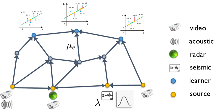
We study experimental design networks, as introduced by Liu at al.ย [1]. In these networks, illustrated in Fig.ย 1, learners and data sources are dispersed across different locations in a network. Learners receive streams of data collected from the sources, and subsequently use them to train models. We are interested in rate allocation strategies that maximize the quality of model training at the learners, subject to network constraints. This problem is of practical significance. For instance, in a smart city [2, 3], various sensors capture, e.g., image, temperature, humidity, traffic, and seismic measurements, which can help forecast transportation traffic, the spread of disease, pollution levels, the weather, etc. Distinct, dispersed public service entities, e.g., a transportation authority, an energy company, the fire department, etc., may perform different training and prediction tasks on these data streams.

Even though the resulting optimization of rate allocations is non-convex, Liu et al.ย [1] provide a polynomial-time $(1-1/e)$-approximation algorithm, exploiting a useful property of the learning objective, namely, continuous DR-submodularity [4, 5]. Thoughย [1] lays a solid foundation for studying this problem, the algorithm proposed suffers from several limitations. First, it is centralized, and requires a full view of network congestion conditions, demand, and learner utilities. This significantly reduces scalability when the number of sources and learners are large. In addition, it uses unicast transmissions between sources and learners. In practice, this significantly under-utilizes network resources when learner interests in data streams overlap.

Refer to caption
Figure 1: An experimental design networkย [1]. Sources (yellow) generate streams of data from diverse sensors, e.g., cameras, microphones, seismic sensors, etc. Learners (blue) train distinct models over (possibly overlapping) received data. We wish to allocate bandwidth to data traffic in a manner that maximizes the social welfare, i.e., the aggregate quality of models across learners.

In this paper, we aim to design efficient algorithms that are (a) distributed and (b) use multicast transmission. Achieving this goal is far from trivial. First, classic decentralization approaches, such as, primal-dual algorithms [6, 7, 8], often operate on (strictly) concave objectives. In contrast, the problem we study here has a non-concave, continuous DR-submodular objective. Second, multicast transmissions naturally result in non-differentiable constraints (see [7, 9], but also Eqs.ย (4) and (6) in Sec.ย III). This further hinders standard decentralization techniques. Our contributions are as follows:

  • โ€ข

    We incorporate multicast transmissions to experimental design networks. This is more realistic when learning jointly from common sensors, and yields a significantly higher throughput in comparison to unicast transmissions.

  • โ€ข

    We prove that, assuming Poisson data streams in steady state and Bayesian linear regression as a learning task, as in [1], our experimental design objective remains continuous DR-submodular.

  • โ€ข

    We construct both centralized and distributed algorithms within a $1-1/e$ factor from the optimal in this setting. For the latter, we make use of a primal dual technique that addresses both the non-differentiability of constituent multicast constraints, as well as the lack of strict convexity exhibited by our problem.

  • โ€ข

    We conduct extensive simulations over both synthetic and backbone network topologies. Our proposed algorithms outperform all competitors w.r.t. the quality of model estimation, and our distributed algorithms perform closely to their centralized versions.

From a technical standpoint, we couple the Frank-Wolfe algorithm by Bian et al.ย [4], also used by Liu et al.ย [1], with a nested distributed step; the latter deals with the non-differentiability of multicast constraints through an $l_{p}$ relaxation of the max norm. We also implement two additional extensions sketched out by Liu et al.ย [1]: we consider (a) Gaussian data sources, that are (b) subject to heterogeneous noise. We incorporate both in our mathematical formulation and theoretically and experimentally characterize performance under these extensions. Gaussianity requires revisiting how gradient estimation is performed, compared to Liu et al., as well as devising new estimation bounds.

The remainder of this paper is organized as follows. Sec.ย II provides a literature review. We introduce our distributed model in Sec.ย III. Sec.ย IV describes our analysis of the problem and proposed centralized algorithm, while Sec.ย V describes our distributed algorithm. We propose additional distributed algorithms in Sec.ย VI. We present numerical experiments in Sec.ย VII, and conclude in Sec.ย VIII.

II Related Work

Experimental Design. As discussed by Liu et al.ย [1], experimental design is classic under a single user with an experiment budget constraintย [10, 11], while the so-called D-Optimality criterion is a popular objectiveย [12, 13, 14, 15, 16]. Liu et al. [1] are the first to extend this objective to the context of experimental design networks. As discussed in the introduction, we deviate from Liu et al.ย by proposing a decentralized algorithm and considering multicast transmissions; both are practically important and come with technical challenges. Liu et al.ย make additional restrictive assumptions, including, e.g., that data samples come from a finite set and that labeling noise is homogeneous across sources, but mention that their analysis could be extended to amend these assumptions. We implement this extension by considering Gaussian sources and noise heteroskedasticity, and proving gradient estimation bounds using appropriate Chernoff inequalities (see, e.g., Lem.ย 1).

Submodular Maximization. Submodularity is traditionally explored within the context of set functions [17], but can also be extended to functions over the integer lattice [5] and the continuous domainย [4]. Maximizing a monotone submodular function subject to a matroid constraint is classic. Krause and Golovin [18] show that the greedy algorithm achieves a $1/2$ approximation ratio. Calinescu et al. [17] propose a continuous greedy algorithm improving the ratio to $1-1/e$ that applies a Frank-Wolfe (FW)ย [19] variant to the multilinear extension of the submodular objective. With the help of auxiliary potential functions, Bian et al.ย [4] show that the same FW variant can be used to maximize continuous DR-submodular functions within a $1-1/e$ ratio. The centralized algorithm by Liu et al.ย [1], and ours, are applications of the FW variantย [4]; in both cases, recovering their guarantees requires devising novel gradient estimators and bounding their estimation accuracy. We also depart by considering a distributed version of this algorithm, where each node accesses only neighborhood knowledge.

Convergence of Primal-Dual Algorithms. Nediฤ‡ and Ozdaglarย [20] propose a subgradient algorithm for generating approximate saddle-point solutions for a convex-concave function. Assuming Slaterโ€™s condition and bounded Lagrangian gradients, they provide bounds on the primal objective function. Alghunaim and Sayed [21] prove linear convergence for primal-dual gradient methods. The methods apply to augmented Lagrangian formulations, whose primal objective is smooth and strongly convex under equality constraints (ours are inequality constraints). Lyapunov equations are usually employed for a continuous version of the primal-dual gradient algorithm [7]; this requires objectives to be strictly concave. Feijer and Paganini [22] prove the stability of primalโ€“dual gradient dynamics with concave objectives through Krasovskiiโ€™s method and the LaSalle invariance principle. We follow [22] to ensure convergence of our decentralized algorithm.

Distributed Algorithms. Distributed algorithms for the maximization of strictly concave objectives under separable constraints are classic (see, e.g., [6, 7, 9, 23]). Our objective is continuous DR-submodular; thus, these methods do not directly extend to our setting. Tychogiorgos et al.ย [24] provide the theoretical foundations for distributed dual algorithm solution of non-convex problems. Mokhtari et al.ย [25] propose a partially decentralized continuous greedy algorithm for DR-submodular maximization subject to down-closed convex constraints and prove a $1-1/e$ guarantee. However, the conditional gradient update step they propose requires global information and remains centralized. Our analysis requires combining above techniques, with the (centralized) Frank-Wolfe variant by Bian et al.ย [4], which yields a $1-1/e$ approximation guarantee. Doing so requires dealing with both the lack of strict convexity of the constituent problem, as well as the non-differentiability of multicast constraints.

III Problem Formulation

Our model, and its exposition below, follows closely Liu et al.ย [1]: for consistency, we use the same notation and terminology. We depart in multiple ways. First and foremost, we (a) seek a distributed algorithm determining the rate allocation, requiring knowledge only from itself and its neighbourhoods, while the centralized algorithm requires global information, and (b) we extend the analysis from unicast to multicast, allowing sharing of the same traffic across learners, thereby increasing throughput. We also implement two potential extensions drafted by Liu et al.ย [1]: we (c) generate features from Gaussian sources instead of a finite set, changing subscripts of variables from feature $\boldsymbol{x}$ to source s๐‘ s, (d) adopt source instead of hop-by-hop routing, which changes the optimized random variables, leading to a general directed graph instead of a DAG (directed acyclic graph), and (f) incorporate heterogeneous noise over source s๐‘ s and types $t$ instead of homogeneous constant noise.

Network. We model the system as a multi-hop network with a topology represented by a directed graph $\mathcal{G}(\mathcal{V},\mathcal{E})$, where $\mathcal{V}$ is the set of nodes and $\mathcal{E}\subset\mathcal{V}\times\mathcal{V}$ is the set of links. Each link $e=(u,v)\in\mathcal{E}$ has a link capacity $\mu^{e}\geq 0$. Sources $\mathcal{S}\subset\mathcal{V}$ generate data streams, while learners $\mathcal{L}\subset\mathcal{V}$ reside at sinks.

Data Sources. Each data source sโˆˆ๐’ฎ๐‘ ๐’ฎs\in\mathcal{S} generates a sequence of labeled pairs $(\boldsymbol{x},y)\in\mathbb{R}^{d}\times\mathbb{R}$ of type $t$ according to a Poisson process of rate ฮปs,tโ‰ฅ0,subscript๐œ†๐‘ ๐‘ก0\lambda_{s,t}\geq 0, corresponding to measurements or experiments the source conducts (each pair is a new measurement). Intuitively, features $\boldsymbol{x}$ correspond to covariates in an experiment (e.g., pixel values in an image, etc.), label types $t\in\mathcal{T}$ correspond to possible measurements (e.g., temperature, radiation level, etc.), and labels $y$ correspond to the actual measurement value collected (e.g., $23^{\circ}\text{C})$.

The generated data follows a linear regression modelย [26, 27], i.e., for every type $t\in\mathcal{T}$ from source sโˆˆ๐’ฎ๐‘ ๐’ฎs\in\mathcal{S}, there exists a $\boldsymbol{\beta}_{t}\in\mathbb{R}^{d}$ such that y=๐’™โŠคโ€‹๐œทt+ฯตs,t๐‘ฆsuperscript๐’™topsubscript๐œท๐‘กsubscriptitalic-ฯต๐‘ ๐‘กy=\boldsymbol{x}^{\top}\boldsymbol{\beta}_{t}+\epsilon_{s,t} where ฯตs,tโˆˆโ„subscriptitalic-ฯต๐‘ ๐‘กโ„\epsilon_{s,t}\in\mathbb{R} are i.i.d.ย zero mean normal noise variables with variance ฯƒs,t2>0subscriptsuperscript๐œŽ2๐‘ ๐‘ก0\sigma^{2}_{s,t}>0. Departing from Liu et al.ย [1], but also from classic experimental design [10], where s๐‘ s samples feature vectors $\boldsymbol{x}\in\mathbb{R}^{d}$ from a finite set, we assume that they are sampled from a Gaussian distribution Nโ€‹(๐ŸŽ,๐šบs)๐‘0subscript๐šบ๐‘ N(\boldsymbol{0},\boldsymbol{\Sigma}_{s}). Again in contrast to [1], we allow for heterogeneous (also known asย heteroskedastic) noise levels ฯƒs,tsubscript๐œŽ๐‘ ๐‘ก\sigma_{s,t} across both sources and experiment types.

Learners and Bayesian Linear Regression. Each learner $\ell\in\mathcal{L}$ wishes to learn a model $\boldsymbol{\beta}_{t^{\ell}}$ for some type $t^{\ell}\in\mathcal{T}$, via Bayesian linear regression. In particular, each $\ell$ has a Gaussian prior $N(\boldsymbol{\beta}_{0}^{\ell},\boldsymbol{\Sigma}_{0}^{\ell})$ on the model $\boldsymbol{\beta}_{t^{\ell}}$ it wishes to estimate. We assume that the system operates for a data acquisition time period $T$. Let nsโ„“โˆˆโ„•superscriptsubscript๐‘›๐‘ โ„“โ„•n_{s}^{\ell}\in\mathbb{N} be the cumulative number of pairs $(\boldsymbol{x},y)$ from source s๐‘ s collected by learner $\ell$ during this period, and ๐’โ„“=[nsโ„“]sโˆˆ๐’ฎsuperscript๐’โ„“subscriptdelimited-[]subscriptsuperscript๐‘›โ„“๐‘ ๐‘ ๐’ฎ\boldsymbol{n}^{\ell}=[n^{\ell}_{s}]_{s\in\mathcal{S}} the vector of arrivals at learner $\ell$ from all sources. We denote by ๐’™s,iโ„“superscriptsubscript๐’™๐‘ ๐‘–โ„“\boldsymbol{x}_{s,i}^{\ell}, ys,iโ„“superscriptsubscript๐‘ฆ๐‘ ๐‘–โ„“y_{s,i}^{\ell} the $i$-th feature and label generated from source s๐‘ s to reach learner $\ell$, and ๐‘ฟโ„“=[[๐’™s,iโ„“]i=1nsโ„“]sโˆˆ๐’ฎsuperscript๐‘ฟโ„“subscriptdelimited-[]superscriptsubscriptdelimited-[]superscriptsubscript๐’™๐‘ ๐‘–โ„“๐‘–1superscriptsubscript๐‘›๐‘ โ„“๐‘ ๐’ฎ\boldsymbol{X}^{\ell}=[[\boldsymbol{x}_{s,i}^{\ell}]_{i=1}^{n_{s}^{\ell}}]_{s\in\mathcal{S}}, ๐’šโ„“=[[ys,iโ„“]i=1nsโ„“]sโˆˆ๐’ฎsuperscript๐’šโ„“subscriptdelimited-[]superscriptsubscriptdelimited-[]superscriptsubscript๐‘ฆ๐‘ ๐‘–โ„“๐‘–1superscriptsubscript๐‘›๐‘ โ„“๐‘ ๐’ฎ\boldsymbol{y}^{\ell}=[[y_{s,i}^{\ell}]_{i=1}^{n_{s}^{\ell}}]_{s\in\mathcal{S}} the feature matrix and label vector, respectively, received at learner $\ell$ up to time $T$. Then, maximum a-posterior (MAP) estimation [27, 1] at learner $\ell$ amounts to:

$\displaystyle\begin{split}\hat{\boldsymbol{\beta}}_{\mathtt{MAP}}^{\ell}=((\boldsymbol{X}^{\ell})^{\top}(\boldsymbol{\tilde{\Sigma}}^{\ell})^{-1}\boldsymbol{X}^{\ell}+(\boldsymbol{\Sigma}_{0}^{\ell})^{-1})^{-1}\cdot\\ ((\boldsymbol{X}^{\ell})^{\top}(\boldsymbol{\tilde{\Sigma}}^{\ell})^{-1}\boldsymbol{y}^{\ell}+(\boldsymbol{\Sigma}_{0}^{\ell})^{-1}\boldsymbol{\beta}_{0}^{\ell}),\end{split}$ (1)

where $\boldsymbol{\tilde{\Sigma}}^{\ell}=\mathbb{R}^{n^{\ell}\times n^{\ell}}$ is a diagonal noise covariance matrix, containing corresponding source noise covariances ฯƒs,tโ„“2superscriptsubscript๐œŽ๐‘ superscript๐‘กโ„“2\sigma_{s,t^{\ell}}^{2} in its diagonal. The quality of this estimator is determined by the error covariance [27], i.e., the $d\times d$ matrix:

$$\mathtt{cov}(\hat{\boldsymbol{\beta}}_{\mathtt{MAP}}^{\ell}-\boldsymbol{\beta}_{t^{\ell}})=\big{(}(\boldsymbol{X}^{\ell})^{\top}(\boldsymbol{\tilde{\Sigma}}^{\ell})^{-1}\boldsymbol{X}^{\ell}+(\boldsymbol{\Sigma}_{0}^{\ell})^{-1}\big{)}^{-1}.$$ (2)

The covariance summarizes the estimator quality in all directions in $\mathbb{R}^{d}$: directions $\boldsymbol{x}\in\mathbb{R}^{d}$ of high variance (e.g., eigenvectors in which eigenvalues of $\mathtt{cov}(\hat{\boldsymbol{\beta}}_{\mathtt{MAP}}^{\ell}-\boldsymbol{\beta}_{t_{\ell}})$ are high) are directions in which the prediction $\hat{y}=\boldsymbol{x}^{\top}\hat{\boldsymbol{\beta}}_{\mathtt{MAP}}^{\ell}$ will have the highest prediction error.

Network Constraints. Data pairs $(\boldsymbol{x},y)\in\mathbb{R}^{d}\times\mathbb{R}$ of type $t\in\mathcal{T}$ generated by sources are transmitted over paths in the network and eventually delivered to learners. Furthermore, we consider the multirate multicast transmissionย [7], which saves network resources compared to unicast. That is, we assume that each source s๐‘ s has a set of paths ๐’ซs,tsubscript๐’ซ๐‘ ๐‘ก\mathcal{P}_{s,t} over which data pairs of type $t$ are routed: each path pโˆˆ๐’ซs,t๐‘subscript๐’ซ๐‘ ๐‘กp\in\mathcal{P}_{s,t} links to a different learner. Note that |๐’ซs,t|subscript๐’ซ๐‘ ๐‘ก|\mathcal{P}_{s,t}|, the size of ๐’ซs,tsubscript๐’ซ๐‘ ๐‘ก\mathcal{P}_{s,t}, equals the number of learners with type $t$. We denote the virtual rateย [7], with which data pairs of type $t$ from source s๐‘ s are transmitted through path pโˆˆ๐’ซs,t๐‘subscript๐’ซ๐‘ ๐‘กp\in\mathcal{P}_{s,t}, as ฮปs,tpโ‰ฅ0.superscriptsubscript๐œ†๐‘ ๐‘ก๐‘0\lambda_{s,t}^{p}\geq 0. Let P๐šƒ๐™พ๐šƒ=โˆ‘sโˆˆ๐’ฎ,tโˆˆ๐’ฏ|๐’ซs,t|subscript๐‘ƒ๐šƒ๐™พ๐šƒsubscriptformulae-sequence๐‘ ๐’ฎ๐‘ก๐’ฏsubscript๐’ซ๐‘ ๐‘กP_{\mathtt{TOT}}=\sum_{s\in\mathcal{S},t\in\mathcal{T}}|\mathcal{P}_{s,t}| be the total number of paths. We refer to the vector

$$\boldsymbol{\lambda}=[\lambda_{s,t}^{p}]_{s\in\mathcal{S},t\in\mathcal{T},p\in\mathcal{P}_{s,t}}\in\mathbb{R}_{+},^{P_{\mathtt{TOT}}}$$ (3)

as the global rates allocation. To satisfy multicast link capacity constraints, for each link $e\in\mathcal{E}$, we must have

โˆ‘sโˆˆ๐’ฎ,tโˆˆ๐’ฏmaxpโˆˆ๐’ซs,t:eโˆˆpโกฮปs,tpโ‰คฮผe.subscriptformulae-sequence๐‘ ๐’ฎ๐‘ก๐’ฏsubscript:๐‘subscript๐’ซ๐‘ ๐‘ก๐‘’๐‘superscriptsubscript๐œ†๐‘ ๐‘ก๐‘superscript๐œ‡๐‘’\sum_{s\in\mathcal{S},t\in\mathcal{T}}\max_{p\in\mathcal{P}_{s,t}:e\in p}\lambda_{s,t}^{p}\leq\mu^{e}. (4)

Note that only data pairs of the same type generated and same source can be multicast together. For learner $l$, we denote by

ฮปsโ„“=ฮปs,tโ„“psuperscriptsubscript๐œ†๐‘ โ„“superscriptsubscript๐œ†๐‘ superscript๐‘กโ„“๐‘\lambda_{s}^{\ell}=\lambda_{s,t^{\ell}}^{p} (5)

the incoming traffic rate of type $t^{\ell}$ at $\ell\in\mathcal{L}$ from source sโˆˆ๐’ฎ๐‘ ๐’ฎs\in\mathcal{S}. Note that pโˆˆ๐’ซs,tโ„“๐‘subscript๐’ซ๐‘ superscript๐‘กโ„“p\in\mathcal{P}_{s,t^{\ell}} and $\ell$ is the last node of $p$. At source s๐‘ s, for each $t\in\mathcal{T}$, we have the constraints:

maxpโˆˆ๐’ซs,tโกฮปs,tpโ‰คฮปs,t.subscript๐‘subscript๐’ซ๐‘ ๐‘กsuperscriptsubscript๐œ†๐‘ ๐‘ก๐‘subscript๐œ†๐‘ ๐‘ก\max_{p\in\mathcal{P}_{s,t}}\lambda_{s,t}^{p}\leq\lambda_{s,t}. (6)

Note that the left hand sides of both constraints in (4) and (6) are non-differentiable. We adopt the following assumption on the network substrate (Asm.ย 1 in [1]):

Assumption 1.

For $\boldsymbol{\lambda}\in\mathcal{D}$, the system is stable and, in steady state, pairs $(\boldsymbol{x},y)\in\mathbb{R}^{d}\times\mathbb{R}$ of type $t^{\ell}$ arrive at learner $\ell\in\mathcal{L}$ according to $|\mathcal{S}|$ independent Poisson processes with rate ฮปsโ„“subscriptsuperscript๐œ†โ„“๐‘ \lambda^{\ell}_{s}.

As discussed in [1], this is satisfied if, e.g., the network is a Kelly networkย [28] where Burkeโ€™s theorem holdsย [27].

D-Optimal Design Objective. The so-called D-optimal design objectiveย [10] for learner $\ell$ is given by:

$$G^{\ell}(\boldsymbol{X}^{\ell},\boldsymbol{n}^{\ell})=\log\det(\mathtt{cov}(\hat{\boldsymbol{\beta}}_{\mathtt{MAP}}^{\ell}-\boldsymbol{\beta}_{t^{\ell}})),$$ (7)

where the covariance is given by Eq.ย (2). As the latter summarises the expected prediction error in all directions, minimizing the $\log\det$ (i.e., the sum of logs of eigenvalues of the covariance) imposes an overall bound on this error.

Aggregate Expected Utility Optimization. Under Asm. 1, the arrivals of pertinent data pairs at learner $\ell$ from source s๐‘ s form a Poisson process with rate ฮปsโ„“superscriptsubscript๐œ†๐‘ โ„“\lambda_{s}^{\ell}. The PMF of arrivals is:

๐โ€‹[๐’โ„“=๐’]=โˆsโˆˆ๐’ฎ(ฮปsโ„“โ€‹T)nsโ„“โ€‹eโˆ’ฮปsโ„“โ€‹Tnsโ„“!,๐delimited-[]superscript๐’โ„“๐’subscriptproduct๐‘ ๐’ฎsuperscriptsuperscriptsubscript๐œ†๐‘ โ„“๐‘‡superscriptsubscript๐‘›๐‘ โ„“superscript๐‘’superscriptsubscript๐œ†๐‘ โ„“๐‘‡superscriptsubscript๐‘›๐‘ โ„“\displaystyle\mathbf{P}[\boldsymbol{n}^{\ell}=\boldsymbol{n}]=\prod_{s\in\mathcal{S}}\frac{(\lambda_{s}^{\ell}T)^{n_{s}^{\ell}}e^{-\lambda_{s}^{\ell}T}}{n_{s}^{\ell}!}, (8)

for all ๐’=[ns]sโˆˆ๐’ฎโˆˆโ„•|๐’ฎ|๐’subscriptdelimited-[]subscript๐‘›๐‘ ๐‘ ๐’ฎsuperscriptโ„•๐’ฎ\boldsymbol{n}=[n_{s}]_{s\in\mathcal{S}}\in\mathbb{N}^{|\mathcal{S}|} and $\ell\in\mathcal{L}$. Then, the PDF (probability distribution function) of features is:

fโ€‹(๐‘ฟโ„“=๐‘ฟ)=โˆsโˆˆ๐’ฎโˆi=1nsโ„“1(2โ€‹ฯ€)d2โ€‹|๐šบs|โ€‹eโˆ’12โ€‹๐’™s,iโŠคโ€‹๐šบsโˆ’1โ€‹๐’™s,i,๐‘“superscript๐‘ฟโ„“๐‘ฟsubscriptproduct๐‘ ๐’ฎsuperscriptsubscriptproduct๐‘–1superscriptsubscript๐‘›๐‘ โ„“1superscript2๐œ‹๐‘‘2subscript๐šบ๐‘ superscript๐‘’12superscriptsubscript๐’™๐‘ ๐‘–topsuperscriptsubscript๐šบ๐‘ 1subscript๐’™๐‘ ๐‘–f(\boldsymbol{X}^{\ell}=\boldsymbol{X})=\prod_{s\in\mathcal{S}}\prod_{i=1}^{n_{s}^{\ell}}\frac{1}{(2\pi)^{\frac{d}{2}}\sqrt{|\boldsymbol{\Sigma}_{s}|}}e^{-\frac{1}{2}\boldsymbol{x}_{s,i}^{\top}\boldsymbol{\Sigma}_{s}^{-1}\boldsymbol{x}_{s,i}}, (9)

for all ๐‘ฟ=[[๐’™s,i]i=1ns]sโˆˆ๐’ฎโˆˆโ„โˆ‘sns๐‘ฟsubscriptdelimited-[]superscriptsubscriptdelimited-[]subscript๐’™๐‘ ๐‘–๐‘–1subscript๐‘›๐‘ ๐‘ ๐’ฎsuperscriptโ„subscript๐‘ subscript๐‘›๐‘ \boldsymbol{X}=[[\boldsymbol{x}_{s,i}]_{i=1}^{n_{s}}]_{s\in\mathcal{S}}\in\mathbb{R}^{\sum_{s}n_{s}} and $\ell\in\mathcal{L}$. We define the utility at learner $\ell\in\mathcal{L}$ as its expected D-optimal design objective, namely:

Uโ„“โ€‹(๐€โ„“)=๐”ผ๐’โ„“โ€‹[๐”ผ๐‘ฟโ„“โ€‹[Gโ„“โ€‹(๐‘ฟโ„“,๐’โ„“)|๐’โ„“]]=โˆ‘๐’โˆˆโ„•|๐’ฎ|๐โ€‹[๐’โ„“=๐’]โ€‹โˆซ๐‘ฟโˆˆโ„โˆ‘snsGโ„“โ€‹(๐‘ฟ,๐’)โ€‹fโ€‹(๐‘ฟโ„“=๐‘ฟ)โ€‹d๐‘ฟ,superscript๐‘ˆโ„“superscript๐€โ„“subscript๐”ผsuperscript๐’โ„“delimited-[]subscript๐”ผsuperscript๐‘ฟโ„“delimited-[]conditionalsuperscript๐บโ„“superscript๐‘ฟโ„“superscript๐’โ„“superscript๐’โ„“subscript๐’superscriptโ„•๐’ฎ๐delimited-[]superscript๐’โ„“๐’subscript๐‘ฟsuperscriptโ„subscript๐‘ subscript๐‘›๐‘ superscript๐บโ„“๐‘ฟ๐’๐‘“superscript๐‘ฟโ„“๐‘ฟdifferential-d๐‘ฟ\displaystyle\begin{split}&U^{\ell}(\boldsymbol{\lambda}^{\ell})=\mathbb{E}_{\boldsymbol{n}^{\ell}}\big{[}\mathbb{E}_{\boldsymbol{X}^{\ell}}[G^{\ell}(\boldsymbol{X}^{\ell},\boldsymbol{n}^{\ell})|\boldsymbol{n}^{\ell}]\big{]}\\ &=\sum_{\boldsymbol{n}\in\mathbb{N}^{|\mathcal{S}|}}\mathbf{P}[\boldsymbol{n}^{\ell}=\boldsymbol{n}]\int_{\boldsymbol{X}\in\mathbb{R}^{\sum_{s}n_{s}}}G^{\ell}(\boldsymbol{X},\boldsymbol{n})f(\boldsymbol{X}^{\ell}=\boldsymbol{X})\mathrm{d}\boldsymbol{X},\end{split}

where ๐€โ„“=[ฮปsโ„“]sโˆˆ๐’ฎsuperscript๐€โ„“subscriptdelimited-[]superscriptsubscript๐œ†๐‘ โ„“๐‘ ๐’ฎ\boldsymbol{\lambda}^{\ell}=[\lambda_{s}^{\ell}]_{s\in\mathcal{S}}, and D-optimal design objective $G^{\ell}$ is given by Eq.ย (7). We wish to solve the following problem:

Maximize: $\displaystyle U(\boldsymbol{\lambda})=\sum_{\ell\in\mathcal{L}}(U^{\ell}(\boldsymbol{\lambda}^{\ell})-U^{\ell}(\mathbf{0})),$ (10a)
s.t. $\displaystyle\boldsymbol{\lambda}\in\mathcal{D},$ (10b)

where $U^{\ell}(\mathbf{0})$ is a lower bound111This is added to ensure the non-negativity of the objective, which is needed to state guarantees in terms of an approximation ratio (c.f.ย Thm.ย 2) [1]. for $U^{\ell}(\boldsymbol{\lambda}^{\ell})$ and feasible set $\mathcal{D}$ is defined by constraints (3)-(6). Note that the feasible set is a down-closed convex set [4]. However, this problem is not convex, as the objective is non-concave.

IV Centralized Algorithm

In this section, we propose a centralized polynomial-time algorithm with a new gradient estimation, as required by the presence of Gaussian sources, to solve Prob. (10). By establishing submodularity, we achieve an optimality guarantee of $1-1/e$.

IV-A DR-submodularity

To solve this non-convex problem, we utilize a key property here: diminishing-returns submodularity, defined as follows:

Definition 1 (DR-Submodularity [4, 5]).

A function $f:\mathbb{N}^{p}\to\mathbb{R}$ is called diminishing-returns (DR) submodular iff for all $\boldsymbol{x},\boldsymbol{y}\in\mathbb{N}^{p}$ such that $\boldsymbol{x}\leq\boldsymbol{y}$ and all $k\in\mathbb{N}$,

$$f(\boldsymbol{x}+k\boldsymbol{e}_{j})-f(\boldsymbol{x})\geq f(\boldsymbol{y}+k\boldsymbol{e}_{j})-f(\boldsymbol{y}),$$ (11)

for all $j=1,\ldots,p$, where $\boldsymbol{e}_{j}$ is the $j$-th standard basis vector. Moreover, if Eq.ย (11) holds for a real valued function $f:\mathbb{R}^{p}_{+}\to\mathbb{R}$ for all $\boldsymbol{x},\boldsymbol{y}\in\mathbb{R}^{p}$ s.t. $\boldsymbol{x}\leq\boldsymbol{y}$ and all $k\in\mathbb{R}_{+}$, the function is called continuous DR-submodular.

The following theorem establishes that objective (10a) is a continuous DR-submodular function.

Theorem 1.

Objective $U(\boldsymbol{\lambda})$ is (a) monotone-increasing and (b) continuous DR-submodular with respect to $\boldsymbol{\lambda}$. Moreover, the partial derivative of $U$ is:

โˆ‚Uโˆ‚ฮปs,tp=โˆ‘n=0โˆžฮ”sโ„“โ€‹(๐€โ„“,n)โ‹…๐โ€‹[nsโ„“=n]โ‹…T,๐‘ˆsuperscriptsubscript๐œ†๐‘ ๐‘ก๐‘superscriptsubscript๐‘›0โ‹…โ‹…superscriptsubscriptฮ”๐‘ โ„“superscript๐€โ„“๐‘›๐delimited-[]superscriptsubscript๐‘›๐‘ โ„“๐‘›๐‘‡\frac{\partial U}{\partial\lambda_{s,t}^{p}}=\sum_{n=0}^{\infty}\Delta_{s}^{\ell}(\boldsymbol{\lambda}^{\ell},n)\cdot\mathbf{P}[n_{s}^{\ell}=n]\cdot T, (12)

where $t=t^{\ell}$, $\ell$ is the last node of $p$, the distribution $\mathrm{P}$ is Poisson described by (8), with parameters governed by ฮปsโ„“โ€‹Tsuperscriptsubscript๐œ†๐‘ โ„“๐‘‡\lambda_{s}^{\ell}T, and

ฮ”sโ„“โ€‹(๐€โ„“,n)=๐”ผ๐’โ„“โ€‹[๐”ผ๐‘ฟโ„“โ€‹[Gโ„“โ€‹(๐‘ฟโ„“,๐’โ„“)|๐’โ„“]|nsโ„“=n+1]โˆ’๐”ผ๐’โ„“โ€‹[๐”ผ๐‘ฟโ„“โ€‹[Gโ€‹(๐‘ฟโ„“,๐’โ„“)|๐’โ„“]|nsโ„“=n].superscriptsubscriptฮ”๐‘ โ„“superscript๐€โ„“๐‘›subscript๐”ผsuperscript๐’โ„“delimited-[]conditionalsubscript๐”ผsuperscript๐‘ฟโ„“delimited-[]conditionalsuperscript๐บโ„“superscript๐‘ฟโ„“superscript๐’โ„“superscript๐’โ„“superscriptsubscript๐‘›๐‘ โ„“๐‘›1subscript๐”ผsuperscript๐’โ„“delimited-[]conditionalsubscript๐”ผsuperscript๐‘ฟโ„“delimited-[]conditional๐บsuperscript๐‘ฟโ„“superscript๐’โ„“superscript๐’โ„“superscriptsubscript๐‘›๐‘ โ„“๐‘›\begin{split}\Delta_{s}^{\ell}(\boldsymbol{\lambda}^{\ell},n)=\mathbb{E}_{\boldsymbol{n}^{\ell}}\left[\mathbb{E}_{\boldsymbol{X}^{\ell}}[G^{\ell}(\boldsymbol{X}^{\ell},\boldsymbol{n}^{\ell})|\boldsymbol{n}^{\ell}]|n_{s}^{\ell}=n+1\right]\\ -\mathbb{E}_{\boldsymbol{n}^{\ell}}\left[\mathbb{E}_{\boldsymbol{X}^{\ell}}[G(\boldsymbol{X}^{\ell},\boldsymbol{n}^{\ell})|\boldsymbol{n}^{\ell}]|n_{s}^{\ell}=n\right].\end{split} (13)

The proof is in App.ย A. Obj.ย (10a) contains two layers of expectations and a different D-optimal design objective fromย [1]. This is a consequence of the Gaussianity and heterogeneity of sources. In turn, this also requires a different argument in establishing the continuous DR-submodularity.

IV-B Algorithm Overview

We follow the Frank-Wolfe variant for monotone continuous DR-submodular function maximization by Bian et al. [4] and Liu et al. [1], but deviate in estimating the gradients of objective $U$. The proposed algorithm is summarized in Alg.ย 1.

Input: $U:\mathcal{D}\to\mathbb{R}_{+}$, $\mathcal{D}$, stepsize $\delta\in(0,1]$.
1 $\boldsymbol{\lambda}^{0}=0,\eta=0,k=0$
2 whileย ฮท<1๐œ‚1\eta<1ย do
3ย ย ย ย ย ย  find direction $\boldsymbol{v}(k)$, s.t. $\boldsymbol{v}(k)=\mathop{\arg\max}_{\boldsymbol{v}\in\mathcal{D}}\langle\boldsymbol{v},\widehat{\nabla U(\boldsymbol{\lambda}(k))}\rangle$
4ย ย ย ย ย ย  ฮณk=minโก{ฮด,1โˆ’ฮท}subscript๐›พ๐‘˜๐›ฟ1๐œ‚\gamma_{k}=\min\{\delta,1-\eta\}
5ย ย ย ย ย ย  ๐€โ€‹(k+1)=๐€โ€‹(k)+ฮณkโ€‹๐’—โ€‹(k)๐€๐‘˜1๐€๐‘˜subscript๐›พ๐‘˜๐’—๐‘˜\boldsymbol{\lambda}(k+1)=\boldsymbol{\lambda}(k)+\gamma_{k}\boldsymbol{v}(k), $\eta=\eta+\gamma_{k}$, $k=k+1$
return $\boldsymbol{\lambda}(K)$
Algorithmย 1 Frank-Wolfe Variant

Frank-Wolfe Variant. Starting from $\boldsymbol{\lambda}(0)=\boldsymbol{0}$, FW iterates:

$\displaystyle\boldsymbol{v}(k)=\mathop{\arg\max}_{\boldsymbol{v}\in\mathcal{D}}\langle\boldsymbol{v},\widehat{\nabla U(\boldsymbol{\lambda}(k))}\rangle,$ (14a)
$\displaystyle\boldsymbol{\lambda}(k+1)=\boldsymbol{\lambda}(k)+\gamma\boldsymbol{v}(k),$ (14b)

where $\widehat{\nabla U(\cdot)}$ is an estimator of the gradient $\nabla U$, and $\gamma$ is an appropriate stepsize. We will further discuss how to estimate the gradient in Sec.ย IV-C. This algorithm achieves a $1-\frac{1}{e}$ approximation guarantee, characterized by:

Theorem 2.

Let $\lambda_{\mathrm{MAX}}=\max_{\boldsymbol{\lambda}\in\mathcal{D}}\|\boldsymbol{\lambda}\|_{1}$. Then, for any $0<\epsilon_{0},\epsilon_{1}<1$, there exists $K=O(\frac{\epsilon_{0}}{P_{\mathtt{TOT}}(|\mathcal{S}|-1)}\epsilon_{1})$, $n^{\prime}=O(\lambda_{\mathrm{MAX}}T+\ln\frac{1}{\epsilon_{1}})$, $N_{1}=N_{2}=\Omega(\sqrt{\ln\frac{P_{\mathtt{TOT}}K}{\epsilon_{0}}\cdot(n^{\prime}+1)}TK)$, s.t., the FW variant algorithm terminates in $K$ iterations, and uses $n^{\prime}$ terms in the sum, $N_{1}$ samples for $\boldsymbol{n}$, and $N_{2}$ samples for $\boldsymbol{X}$ in estimator (17). Thus, with probability greater than $1-\epsilon_{0}$, the output solution $\boldsymbol{\lambda}(K)\in\mathcal{D}$ of Alg.ย 1 satisfies:

$$U(\boldsymbol{\lambda}(K))\geq(1-e^{\epsilon_{1}-1})\max_{\boldsymbol{\lambda}\in\mathcal{D}}U(\boldsymbol{\lambda})-\epsilon_{2},$$ (15)

where $\epsilon_{2}$ determined by $\epsilon_{0},\epsilon_{1}$ and network parameters: ฯต2=(T2โ€‹P๐šƒ๐™พ๐šƒโ€‹ฮปMAX2+2โ€‹ฮปMAX)โ€‹1Kโ€‹maxโ„“โˆˆโ„’,sโˆˆ๐’ฎโกlogโก(1+ฮปMAXโ€‹(๐šบ0โ„“)โ€‹cs2ฯƒs,t2)>0subscriptitalic-ฯต2superscript๐‘‡2subscript๐‘ƒ๐šƒ๐™พ๐šƒsuperscriptsubscript๐œ†MAX22subscript๐œ†MAX1๐พsubscriptformulae-sequenceโ„“โ„’๐‘ ๐’ฎ1subscript๐œ†MAXsuperscriptsubscript๐šบ0โ„“superscriptsubscript๐‘๐‘ 2superscriptsubscript๐œŽ๐‘ ๐‘ก20\epsilon_{2}=(T^{2}P_{\mathtt{TOT}}\lambda_{\mathrm{MAX}}^{2}+2\lambda_{\mathrm{MAX}})\frac{1}{K}\max_{\ell\in\mathcal{L},s\in\mathcal{S}}\log\left(1+\frac{\lambda_{\mathrm{MAX}}(\boldsymbol{\Sigma}_{0}^{\ell})c_{s}^{2}}{\sigma_{s,t}^{2}}\right)>0, cs=4โ€‹ฮปMAXโ€‹(๐šบs)โ€‹d+2โ€‹ฮปMAXโ€‹(๐šบs)โ€‹logโก1ฮดsubscript๐‘๐‘ 4subscript๐œ†MAXsubscript๐šบ๐‘ ๐‘‘2subscript๐œ†MAXsubscript๐šบ๐‘ 1๐›ฟc_{s}=4\sqrt{\lambda_{\mathrm{MAX}}(\boldsymbol{\Sigma}_{s})}\sqrt{d}+2\sqrt{\lambda_{\mathrm{MAX}}(\boldsymbol{\Sigma}_{s})}\sqrt{\log\frac{1}{\delta}}, and $\delta=O\left(\frac{\epsilon_{0}}{P_{\mathtt{TOT}}K|\mathcal{S}|n^{\prime}}\right)$.

The proof is in App.ย C. Our algorithm is based on the Frank-Wolfe variant from Bian et al. [4]. Similar to Thm.ย 2 in [1], our guarantee involves gradient estimation through truncating and sampling, due to Poisson arrivals (see Asm.ย 1). However, incorporating Gaussian sources, we need to also sample from the Gaussian distribution to ensure a polynomial-time estimator. This requires combining a sub-Gaussian norm bound [29] with the aforementioned truncating and sampling techniques.

IV-C Gradient Estimation

We describe here how to produce an unbiased, polynomial-time estimator of our gradient $\widehat{\nabla U}$, which is accessed by Eq.ย (14a). There are three challenges in computing the true gradient (12): (a) the outer sum involves infinite summation over nsโ„“โˆˆโ„•superscriptsubscript๐‘›๐‘ โ„“โ„•n_{s}^{\ell}\in\mathbb{N}; (b) the outer expectation involves an exponential sum in $|\mathcal{S}|-1$; and (c) the inner expectation involves an exponential sum in $\|\boldsymbol{n}^{\ell}\|$. The last arises from Gaussian sources, which differs from gradient estimation inย [1]; this requires the use of a different bound (see Lem.ย 7 in the Appendix), as well as a decoupling argument (as features and arrivals are jointly distributed).

To address these challenges, we (a) truncate the infinite summation while maintaining the quality of estimation through a Poisson tail bound:

HEADs,tpโ€‹(nโ€ฒ)=โˆ‘n=0nโ€ฒฮ”sโ„“โ€‹(๐€โ„“,n)โ‹…๐โ€‹[nsโ„“=n]โ‹…T,superscriptsubscriptHEAD๐‘ ๐‘ก๐‘superscript๐‘›โ€ฒsuperscriptsubscript๐‘›0superscript๐‘›โ€ฒโ‹…โ‹…superscriptsubscriptฮ”๐‘ โ„“superscript๐€โ„“๐‘›๐delimited-[]superscriptsubscript๐‘›๐‘ โ„“๐‘›๐‘‡\mathrm{HEAD}_{s,t}^{p}(n^{\prime})=\sum_{n=0}^{n^{\prime}}\Delta_{s}^{\ell}(\boldsymbol{\lambda}^{\ell},n)\cdot\mathbf{P}[n_{s}^{\ell}=n]\cdot T, (16)

where $t=t^{\ell}$, $l$ is the last node of $p$, ฮ”sโ„“โ€‹(๐€โ„“,n)superscriptsubscriptฮ”๐‘ โ„“superscript๐€โ„“๐‘›\Delta_{s}^{\ell}(\boldsymbol{\lambda}^{\ell},n) is defined in Eq.ย (13), and $n^{\prime}$ is the truncating parameter. We then (b) sample $\boldsymbol{n}^{\ell}$ ($N_{1}$ samples) according to the Poisson distribution, parameterized by $\boldsymbol{\lambda}^{\ell}T$; and (c) sample $\boldsymbol{X}^{\ell}$ ($N_{2}$ samples) according to the Gaussian distribution. When nโ€ฒโ‰ฅฮปsโ„“โ€‹Tsuperscript๐‘›โ€ฒsuperscriptsubscript๐œ†๐‘ โ„“๐‘‡n^{\prime}\geq\lambda_{s}^{\ell}T, we estimate the gradient by polynomial-time sampling:

โˆ‚Uโˆ‚ฮปs,tp^=โˆ‘n=0nโ€ฒฮ”sโ„“โ€‹(๐€โ„“,n)^โ‹…๐โ€‹[nsโ„“=n]โ‹…T,^๐‘ˆsuperscriptsubscript๐œ†๐‘ ๐‘ก๐‘superscriptsubscript๐‘›0superscript๐‘›โ€ฒโ‹…โ‹…^superscriptsubscriptฮ”๐‘ โ„“superscript๐€โ„“๐‘›๐delimited-[]superscriptsubscript๐‘›๐‘ โ„“๐‘›๐‘‡\displaystyle\widehat{\frac{\partial U}{\partial\lambda_{s,t}^{p}}}=\sum_{n=0}^{n^{\prime}}\widehat{\Delta_{s}^{\ell}(\boldsymbol{\lambda}^{\ell},n)}\cdot\mathbf{P}[n_{s}^{\ell}=n]\cdot T, (17)

where

ฮ”sโ„“โ€‹(๐€โ„“,n)^=1N1โ€‹N2โˆ‘j=1N1โˆ‘k=1N2(Gโ„“(๐‘ฟโ„“,j,k,๐’โ„“,j|nsโ„“,j=n+1)โˆ’Gโ„“(๐‘ฟโ„“,j,k,๐’โ„“,j|nsโ„“,j=n)),^superscriptsubscriptฮ”๐‘ โ„“superscript๐€โ„“๐‘›1subscript๐‘1subscript๐‘2superscriptsubscript๐‘—1subscript๐‘1superscriptsubscript๐‘˜1subscript๐‘2superscript๐บโ„“superscript๐‘ฟโ„“๐‘—๐‘˜evaluated-atsuperscript๐’โ„“๐‘—superscriptsubscript๐‘›๐‘ โ„“๐‘—๐‘›1superscript๐บโ„“superscript๐‘ฟโ„“๐‘—๐‘˜evaluated-atsuperscript๐’โ„“๐‘—superscriptsubscript๐‘›๐‘ โ„“๐‘—๐‘›\begin{split}\widehat{\Delta_{s}^{\ell}(\boldsymbol{\lambda}^{\ell},n)}=\frac{1}{N_{1}N_{2}}\sum_{j=1}^{N_{1}}\sum_{k=1}^{N_{2}}(G^{\ell}(\boldsymbol{X}^{\ell,j,k},\boldsymbol{n}^{\ell,j}|_{n_{s}^{\ell,j}=n+1})-\\ G^{\ell}(\boldsymbol{X}^{\ell,j,k},\boldsymbol{n}^{\ell,j}|_{n_{s}^{\ell,j}=n})),\end{split}

๐’j|nsโ„“,j=nevaluated-atsuperscript๐’๐‘—superscriptsubscript๐‘›๐‘ โ„“๐‘—๐‘›\boldsymbol{n}^{j}|_{n_{s}^{\ell,j}=n} indicates vector $\boldsymbol{n}^{j}$ with nsโ„“,j=nsuperscriptsubscript๐‘›๐‘ โ„“๐‘—๐‘›n_{s}^{\ell,j}=n, and $N_{1}$, $N_{2}$ are sampling parameters. At each iteration, we generate $N_{1}$ samples $\boldsymbol{n}^{\ell,j}$, $j=1,\dots,N_{1}$ of the random vector $\boldsymbol{n}^{\ell}$ according to the Poisson distribution in Eq.ย (8), parameterized by the current solution vector $\boldsymbol{\lambda}^{\ell}T$. Having a sample $\boldsymbol{n}^{\ell,j}$, we could sample $N_{2}$ samples $\boldsymbol{X}^{\ell,j,k}$, $k=1,\dots,N_{2}$ of random matrix ๐‘ฟโ„“,j=[[๐’™s,iโ„“]i=1nsโ„“,j]sโˆˆ๐’ฎsuperscript๐‘ฟโ„“๐‘—subscriptdelimited-[]superscriptsubscriptdelimited-[]subscriptsuperscript๐’™โ„“๐‘ ๐‘–๐‘–1subscriptsuperscript๐‘›โ„“๐‘—๐‘ ๐‘ ๐’ฎ\boldsymbol{X}^{\ell,j}=[[\boldsymbol{x}^{\ell}_{s,i}]_{i=1}^{n^{\ell,j}_{s}}]_{s\in\mathcal{S}} according to the Gaussian distribution in Eq.ย (9). We bound the distance between the estimated and true gradient as follows:

Lemma 1.

For any $\delta\in(0,1)$, and nโ€ฒโ‰ฅฮปsโ„“โ€‹Tsuperscript๐‘›โ€ฒsuperscriptsubscript๐œ†๐‘ โ„“๐‘‡n^{\prime}\geq\lambda_{s}^{\ell}T,

โˆ’ฮณโ€‹maxโ„“โˆˆโ„’,sโˆˆ๐’ฎโกlogโก(1+ฮปMAXโ€‹(๐šบ0โ„“)โ€‹cs2ฯƒs,t2)โ‰คโˆ‚Uโˆ‚ฮปs,tpโˆ’โˆ‚Uโˆ‚ฮปs,tp^โ‰คฮณโ€‹maxโ„“โˆˆโ„’,sโˆˆ๐’ฎโกlogโก(1+ฮปMAXโ€‹(๐šบ0โ„“)โ€‹cs2ฯƒs,t2)+๐โ€‹[nsโ„“โ‰ฅnโ€ฒ+1]โ€‹โˆ‚Uโˆ‚ฮปs,tp,๐›พsubscriptformulae-sequenceโ„“โ„’๐‘ ๐’ฎ1subscript๐œ†MAXsuperscriptsubscript๐šบ0โ„“superscriptsubscript๐‘๐‘ 2superscriptsubscript๐œŽ๐‘ ๐‘ก2๐‘ˆsuperscriptsubscript๐œ†๐‘ ๐‘ก๐‘^๐‘ˆsuperscriptsubscript๐œ†๐‘ ๐‘ก๐‘๐›พsubscriptformulae-sequenceโ„“โ„’๐‘ ๐’ฎ1subscript๐œ†MAXsuperscriptsubscript๐šบ0โ„“superscriptsubscript๐‘๐‘ 2superscriptsubscript๐œŽ๐‘ ๐‘ก2๐delimited-[]subscriptsuperscript๐‘›โ„“๐‘ superscript๐‘›โ€ฒ1๐‘ˆsuperscriptsubscript๐œ†๐‘ ๐‘ก๐‘\begin{split}-\gamma\max_{\ell\in\mathcal{L},s\in\mathcal{S}}\log(1+\frac{\lambda_{\mathrm{MAX}}(\boldsymbol{\Sigma}_{0}^{\ell})c_{s}^{2}}{\sigma_{s,t}^{2}})\leq\frac{\partial U}{\partial\lambda_{s,t}^{p}}-\widehat{\frac{\partial U}{\partial\lambda_{s,t}^{p}}}\leq\\ \gamma\max_{\ell\in\mathcal{L},s\in\mathcal{S}}\log(1+\frac{\lambda_{\mathrm{MAX}}(\boldsymbol{\Sigma}_{0}^{\ell})c_{s}^{2}}{\sigma_{s,t}^{2}})+\mathbf{P}[n^{\ell}_{s}\geq n^{\prime}+1]\frac{\partial U}{\partial\lambda_{s,t}^{p}},\end{split}

with probability greater than 1โˆ’2โ‹…eโˆ’ฮณ2โ€‹N1โ€‹N2/2โ€‹T2โ€‹(nโ€ฒ+1)โˆ’|๐’ฎ|โ€‹nโ€ฒโ€‹ฮดโˆ’(|๐’ฎ|โˆ’1)โ€‹ฮดs,tp1โ‹…2superscript๐‘’superscript๐›พ2subscript๐‘1subscript๐‘22superscript๐‘‡2superscript๐‘›โ€ฒ1๐’ฎsuperscript๐‘›โ€ฒ๐›ฟ๐’ฎ1superscriptsubscript๐›ฟ๐‘ ๐‘ก๐‘1-2\cdot e^{-\gamma^{2}N_{1}N_{2}/2T^{2}(n^{\prime}+1)}-|\mathcal{S}|n^{\prime}\delta-(|\mathcal{S}|-1)\delta_{s,t}^{p}, where $\lambda_{\mathrm{MAX}}(\boldsymbol{\Sigma}_{0}^{\ell})$ is the maximum eigenvalue of matrix $\boldsymbol{\Sigma}_{0}^{\ell}$.

The proof is in App.ย B. Combining this estimated gradient in Eq.ย (17) with classic Frank-Wolfe variant [4], we propose Alg.ย (14) and establish Thm.ย 2.

V Distributed Algorithm

Implementing Alg. (14) in our distributed learning network is hard, as it requires the full knowledge of the network. We thus present our distributed algorithm for solving Prob. (10). The algorithm performs a primal dual gradient algorithm over a modified Lagrangian to effectively find direction $\boldsymbol{v}$, defined in Eq.ย (14a), in a distributed fashion. The linearity of Eq.ย (14a) ensures convergence, while Thm.ย 2 ensures the aggregate utility attained in steady state is within an $1-\frac{1}{e}$ factor from the optimal.

V-A Algorithm Overview

Solving Prob.ย (10) in a distributed fashion requires decentralizing Eqs.ย (14a) and (14b). Decentralizing the latter is easy, as Eq. (14b) can be executed across sources via:

ฮปs,tpโ€‹(k+1)=ฮปs,tpโ€‹(k)+ฮณโ€‹vs,tpโ€‹(k),superscriptsubscript๐œ†๐‘ ๐‘ก๐‘๐‘˜1superscriptsubscript๐œ†๐‘ ๐‘ก๐‘๐‘˜๐›พsuperscriptsubscript๐‘ฃ๐‘ ๐‘ก๐‘๐‘˜\displaystyle\lambda_{s,t}^{p}(k+1)=\lambda_{s,t}^{p}(k)+\gamma v_{s,t}^{p}(k), (18)

across all sโˆˆ๐’ฎ๐‘ ๐’ฎs\in\mathcal{S}, and for all $t\in\mathcal{T}$, pโˆˆ๐’ซs,t๐‘subscript๐’ซ๐‘ ๐‘กp\in\mathcal{P}_{s,t}. We thus turn our attention to decentralizing Eq.ย (14a).

Eq.ย (14a) is a linear program. Standard primal-dual distributed algorithms (see, e.g.,ย [7, 9]) typically require strictly concave objectives, as they otherwise would yield to harmonic oscillations and not converge to an optimal pointย [22] in linear programs. An additional challenge arises from the multicast constraints in Eqs.ย (4) and (6): the $\max$ function is non-differentiable. The maximum could be replaced by a set of multiple inequality constraints, but this approach does not scale well, introducing a new dual variable per additional constraint.

To address the first challenge, we follow Feijer and Paganiniย [22] and replace constraints of the form $u\leq 0$ with $\phi(u)\leq 0$, where $\phi(u)=e^{u}-1$. In order to obtain a scalable differentiable Lagrangian, we use the approach in [7, 9]: we replace the multicast constraints (4) and (6) by

โˆ‘sโˆˆ๐’ฎ,tโˆˆ๐’ฏ(โˆ‘pโˆˆ๐’ซs,t:eโˆˆp(vs,tp)ฮธ)1ฮธโ‰คฮผe,subscriptformulae-sequence๐‘ ๐’ฎ๐‘ก๐’ฏsuperscriptsubscript:๐‘subscript๐’ซ๐‘ ๐‘ก๐‘’๐‘superscriptsuperscriptsubscript๐‘ฃ๐‘ ๐‘ก๐‘๐œƒ1๐œƒsuperscript๐œ‡๐‘’\sum_{s\in\mathcal{S},t\in\mathcal{T}}\left(\sum_{p\in\mathcal{P}_{s,t}:e\in p}(v_{s,t}^{p})^{\theta}\right)^{\frac{1}{\theta}}\leq\mu^{e}, (19)

for each link $e\in\mathcal{E}$, and

(โˆ‘pโˆˆ๐’ซs,t:eโˆˆp(vs,tp)ฮธ)1ฮธโ‰คฮปs,t,superscriptsubscript:๐‘subscript๐’ซ๐‘ ๐‘ก๐‘’๐‘superscriptsuperscriptsubscript๐‘ฃ๐‘ ๐‘ก๐‘๐œƒ1๐œƒsubscript๐œ†๐‘ ๐‘ก\left(\sum_{p\in\mathcal{P}_{s,t}:e\in p}(v_{s,t}^{p})^{\theta}\right)^{\frac{1}{\theta}}\leq\lambda_{s,t}, (20)

for each source sโˆˆ๐’ฎ๐‘ ๐’ฎs\in\mathcal{S} and each type $t\in\mathcal{T}$. Note that this is tantamount to approximating $\|\cdot\|_{\infty}$ with $\|\cdot\|_{\theta}$. Combining these two approaches together, the Lagrangian for the modified problem is:

Lโ€‹(๐’—,๐’’,๐’“,๐’–)=โŸจ๐’—,โˆ‡Uโ€‹(๐€)^โŸฉโˆ’โˆ‘eโˆˆโ„ฐqeโ€‹(egeโ€‹(๐’—)โˆ’1)โˆ’โˆ‘sโˆˆ๐’ฎ,tโˆˆ๐’ฏrs,tโ€‹(egs,tโ€‹(๐’—)โˆ’1)โˆ’โˆ‘sโˆˆ๐’ฎ,tโˆˆ๐’ฏโˆ‘pโˆˆ๐’ซs,tus,tpโ€‹(egs,tpโ€‹(๐’—)โˆ’1),๐ฟ๐’—๐’’๐’“๐’–๐’—^โˆ‡๐‘ˆ๐€subscript๐‘’โ„ฐsubscript๐‘ž๐‘’superscript๐‘’subscript๐‘”๐‘’๐’—1subscriptformulae-sequence๐‘ ๐’ฎ๐‘ก๐’ฏsubscript๐‘Ÿ๐‘ ๐‘กsuperscript๐‘’subscript๐‘”๐‘ ๐‘ก๐’—1subscriptformulae-sequence๐‘ ๐’ฎ๐‘ก๐’ฏsubscript๐‘subscript๐’ซ๐‘ ๐‘กsuperscriptsubscript๐‘ข๐‘ ๐‘ก๐‘superscript๐‘’superscriptsubscript๐‘”๐‘ ๐‘ก๐‘๐’—1\begin{split}&L(\boldsymbol{v},\boldsymbol{q},\boldsymbol{r},\boldsymbol{u})=\langle\boldsymbol{v},\widehat{\nabla U(\boldsymbol{\lambda})}\rangle-\sum_{e\in\mathcal{E}}q_{e}(e^{g_{e}(\boldsymbol{v})}-1)-\sum_{s\in\mathcal{S},t\in\mathcal{T}}\\ &r_{s,t}(e^{g_{s,t}}(\boldsymbol{v})-1)-\sum_{s\in\mathcal{S},t\in\mathcal{T}}\sum_{p\in\mathcal{P}_{s,t}}u_{s,t}^{p}(e^{g_{s,t}^{p}(\boldsymbol{v})}-1),\end{split}

where

geโ€‹(๐’—)=โˆ‘sโˆˆ๐’ฎ,tโˆˆ๐’ฏ(โˆ‘pโˆˆ๐’ซs,t:eโˆˆp(vs,tp)ฮธ)1ฮธโˆ’ฮผe,subscript๐‘”๐‘’๐’—subscriptformulae-sequence๐‘ ๐’ฎ๐‘ก๐’ฏsuperscriptsubscript:๐‘subscript๐’ซ๐‘ ๐‘ก๐‘’๐‘superscriptsuperscriptsubscript๐‘ฃ๐‘ ๐‘ก๐‘๐œƒ1๐œƒsuperscript๐œ‡๐‘’\displaystyle g_{e}(\boldsymbol{v})=\sum_{s\in\mathcal{S},t\in\mathcal{T}}\left(\sum_{p\in\mathcal{P}_{s,t}:e\in p}(v_{s,t}^{p})^{\theta}\right)^{\frac{1}{\theta}}-\mu^{e},
gs,tโ€‹(๐’—)=โˆ‘pโˆˆ๐’ซs,t(โˆ‘pโˆˆ๐’ซs,t:eโˆˆp(vs,tp)ฮธ)1ฮธโˆ’ฮปs,t,subscript๐‘”๐‘ ๐‘ก๐’—subscript๐‘subscript๐’ซ๐‘ ๐‘กsuperscriptsubscript:๐‘subscript๐’ซ๐‘ ๐‘ก๐‘’๐‘superscriptsuperscriptsubscript๐‘ฃ๐‘ ๐‘ก๐‘๐œƒ1๐œƒsubscript๐œ†๐‘ ๐‘ก\displaystyle g_{s,t}(\boldsymbol{v})=\sum_{p\in\mathcal{P}_{s,t}}\left(\sum_{p\in\mathcal{P}_{s,t}:e\in p}(v_{s,t}^{p})^{\theta}\right)^{\frac{1}{\theta}}-\lambda_{s,t},
gs,tpโ€‹(๐’—)=โˆ’vs,tp,superscriptsubscript๐‘”๐‘ ๐‘ก๐‘๐’—superscriptsubscript๐‘ฃ๐‘ ๐‘ก๐‘\displaystyle g_{s,t}^{p}(\boldsymbol{v})=-v_{s,t}^{p},

and $\boldsymbol{q}=[q_{e}]_{e\in\mathcal{E}}$, ๐’“=[rs,t]sโˆˆ๐’ฎ,tโˆˆ๐’ฏ๐’“subscriptdelimited-[]subscript๐‘Ÿ๐‘ ๐‘กformulae-sequence๐‘ ๐’ฎ๐‘ก๐’ฏ\boldsymbol{r}=[r_{s,t}]_{s\in\mathcal{S},t\in\mathcal{T}}, and ๐’–=[us,tp]sโˆˆ๐’ฎ,tโˆˆ๐’ฏ,pโˆˆ๐’ซs,t๐’–subscriptdelimited-[]superscriptsubscript๐‘ข๐‘ ๐‘ก๐‘formulae-sequence๐‘ ๐’ฎformulae-sequence๐‘ก๐’ฏ๐‘subscript๐’ซ๐‘ ๐‘ก\boldsymbol{u}=[u_{s,t}^{p}]_{s\in\mathcal{S},t\in\mathcal{T},p\in\mathcal{P}_{s,t}} are non-negative dual variables. Intuitively, $L$ penalizes the infeasibility of network constraints.

We apply a primal dual gradient algorithm over this modified Lagrangian to decentralize Eq.ย (14a). In particular, at iteration $\tau+1$, the primal variables are adjusted via gradient ascent:

vs,tpโ€‹(ฯ„+1)=vs,tpโ€‹(ฯ„)+ms,tpโ€‹โˆ‡vs,tpLโ€‹(ฯ„),superscriptsubscript๐‘ฃ๐‘ ๐‘ก๐‘๐œ1superscriptsubscript๐‘ฃ๐‘ ๐‘ก๐‘๐œsuperscriptsubscript๐‘š๐‘ ๐‘ก๐‘subscriptโˆ‡superscriptsubscript๐‘ฃ๐‘ ๐‘ก๐‘๐ฟ๐œv_{s,t}^{p}(\tau+1)=v_{s,t}^{p}(\tau)+m_{s,t}^{p}\nabla_{v_{s,t}^{p}}L(\tau), (21)

and the dual variables are adjusted via gradient descent:

$\displaystyle q_{e}(\tau+1)=q_{e}(\tau)-k_{e}(\nabla_{q_{e}}L(\tau))_{q_{e}(\tau)}^{+},$ (22a)
$\displaystyle r_{s,t}(\tau+1)=r_{s,t}(\tau)-h_{s,t}(\nabla_{r_{s,t}}L(\tau))_{q_{e}(\tau)})_{r_{s,t}(\tau)}^{+},$ (22b)
$\displaystyle u_{s,t}^{p}(\tau+1)=u_{s,t}^{p}(\tau)-w_{s,t}^{p}(\nabla_{u_{s,t}^{p}}L(\tau))_{q_{e}(\tau)})_{u_{s,t}^{p}(\tau)}^{+},$ (22c)

for each edge $e\in\mathcal{E}$, source sโˆˆ๐’ฎ๐‘ ๐’ฎs\in\mathcal{S}, type $t\in\mathcal{T}$, and path pโˆˆ๐’ซs,t๐‘subscript๐’ซ๐‘ ๐‘กp\in\mathcal{P}_{s,t}, where $k_{e}>0$, hs,t>0subscriptโ„Ž๐‘ ๐‘ก0h_{s,t}>0, ws,tp>0superscriptsubscript๐‘ค๐‘ ๐‘ก๐‘0w_{s,t}^{p}>0, and ms,tp>0superscriptsubscript๐‘š๐‘ ๐‘ก๐‘0m_{s,t}^{p}>0 are stepsize for $q_{e}$, rs,tsubscript๐‘Ÿ๐‘ ๐‘กr_{s,t}, us,tpsuperscriptsubscript๐‘ข๐‘ ๐‘ก๐‘u_{s,t}^{p} and vs,tpsuperscriptsubscript๐‘ฃ๐‘ ๐‘ก๐‘v_{s,t}^{p}, respectively, and $(y)_{x}^{+}=\begin{cases}y,&x>0,\\ \max(y,0),&x\leq 0.\end{cases}$ These operations can indeed be distributed across the network, as we describe in Sec.ย V-B. The following theorem states the convergence of this modified primal dual gradient algorithm, according to Thm.ย 11 in [22]:

Theorem 3.

The trajectories of the modified primalโ€“dual gradient algorithm (Eqs.ย (21) and (22)), with constant stepsize, converge to $\boldsymbol{v}^{*}_{\theta}$. The $\boldsymbol{v}^{*}_{\theta}$ is an optimum of Prob.ย (14a) over $\mathcal{D}_{\theta}$, where $\mathcal{D}_{\theta}$ is $\mathcal{D}$ with (4) replaced byย (19).

For $\boldsymbol{v}^{*}$ be the optimum of Eq. (14a), $\lim_{\theta\to\infty}\boldsymbol{v}^{*}_{\theta}\to\boldsymbol{v}^{*}$, as $\mathcal{D}_{\theta}\to\mathcal{D}$. Thus, our distributed algorithm preserves a $1-\frac{1}{e}$ approximation factor from the optimal objective value as stated in Thm.ย 2, for large enough $\theta$.

$v_{s,t}^{p}(\tau+1)=v_{s,t}^{p}(\tau)+m_{s,t}^{p}\left(\nabla_{\lambda_{s,t}^{p}}U(\boldsymbol{\lambda})-\sum_{e\in p}q_{e}(\tau)\cdot\right.e^{\sum_{s^{\prime}\in\mathcal{S},t^{\prime}\in\mathcal{T}}(v_{s^{\prime},t^{\prime}}^{e}(\tau))^{\frac{1}{\theta}}-\mu^{e}}(v_{s,t}^{e}(\tau))^{\frac{1-\theta}{\theta}}(v_{s,t}^{p}(\tau))^{\theta-1}-$ (I.1)
$r_{s,t}e^{\left(\sum_{p\in\mathcal{P}_{s,t}}(v_{s,t}^{p}(\tau))^{\theta}\right)^{\frac{1}{\theta}}-\lambda_{s,t}}\left(\sum_{p\in\mathcal{P}_{s,t}}(v_{s,t}^{p}(\tau))^{\theta}\right)^{\frac{1-\theta}{\theta}}\left.(v_{s,t}^{p}(\tau))^{\theta-1}+u_{s,t}^{p}\exp(-v_{s,t}^{p}(\tau))\right)$.
vs,teโ€‹(ฯ„)=โˆ‘pโˆˆ๐’ซs,t:eโˆˆp(vs,tpโ€‹(ฯ„))ฮธsuperscriptsubscript๐‘ฃ๐‘ ๐‘ก๐‘’๐œsubscript:๐‘subscript๐’ซ๐‘ ๐‘ก๐‘’๐‘superscriptsuperscriptsubscript๐‘ฃ๐‘ ๐‘ก๐‘๐œ๐œƒv_{s,t}^{e}(\tau)=\sum_{p\in\mathcal{P}_{s,t}:e\in p}(v_{s,t}^{p}(\tau))^{\theta}. (I.2)
qeโ€‹(ฯ„+1)=qeโ€‹(ฯ„)+keโ€‹(eโˆ‘sโˆˆ๐’ฎ,tโˆˆ๐’ฏ(vs,teโ€‹(ฯ„))1ฮธโˆ’ฮผeโˆ’1)qeโ€‹(ฯ„)+subscript๐‘ž๐‘’๐œ1subscript๐‘ž๐‘’๐œsubscript๐‘˜๐‘’superscriptsubscriptsuperscript๐‘’subscriptformulae-sequence๐‘ ๐’ฎ๐‘ก๐’ฏsuperscriptsuperscriptsubscript๐‘ฃ๐‘ ๐‘ก๐‘’๐œ1๐œƒsuperscript๐œ‡๐‘’1subscript๐‘ž๐‘’๐œq_{e}(\tau+1)=q_{e}(\tau)+k_{e}\big{(}e^{\sum_{s\in\mathcal{S},t\in\mathcal{T}}(v_{s,t}^{e}(\tau))^{\frac{1}{\theta}}\!-\!\mu^{e}}\!-\!1\big{)}_{q_{e}(\tau)}^{+}. (I.3)
rs,tโ€‹(ฯ„+1)=rs,tโ€‹(ฯ„)+hs,tโ€‹(e(โˆ‘pโˆˆ๐’ซs,t(vs,tpโ€‹(ฯ„))ฮธ)1ฮธโˆ’ฮปs,tโˆ’1)rs,tโ€‹(ฯ„)+subscript๐‘Ÿ๐‘ ๐‘ก๐œ1subscript๐‘Ÿ๐‘ ๐‘ก๐œsubscriptโ„Ž๐‘ ๐‘กsuperscriptsubscriptsuperscript๐‘’superscriptsubscript๐‘subscript๐’ซ๐‘ ๐‘กsuperscriptsuperscriptsubscript๐‘ฃ๐‘ ๐‘ก๐‘๐œ๐œƒ1๐œƒsubscript๐œ†๐‘ ๐‘ก1subscript๐‘Ÿ๐‘ ๐‘ก๐œr_{s,t}(\tau+1)=r_{s,t}(\tau)+h_{s,t}\left(e^{\left(\sum_{p\in\mathcal{P}_{s,t}}(v_{s,t}^{p}(\tau))^{\theta}\right)^{\frac{1}{\theta}}-\lambda_{s,t}}-1\right)_{r_{s,t}(\tau)}^{+}. (I.4)
$u_{s,t}^{p}(\tau+1)=u_{s,t}^{p}(\tau)+w_{s,t}^{p}\left(e^{-v_{s,t}^{p}(\tau)})-1\right)_{u_{s,t}^{p}(\tau)}^{+}$. (I.5)
TABLE I: Expanding primal and dual steps in Eqs.ย (21) and (22), so that we can execute FW algorithm distributively.

V-B Distributed FW Implementation Details

We conclude by giving the full implementation details of the distributed FW algorithm and, in particular, the primal dual steps, describing the state maintained by every node, the messages exchanged, and the constituent state adaptations. Starting from $\boldsymbol{\lambda}(0)=\boldsymbol{0}$, the algorithm iterates over:

  1. 1.

    Each source node sโˆˆ๐’ฎ๐‘ ๐’ฎs\in\mathcal{S} finds direction vs,tpโ€‹(k)superscriptsubscript๐‘ฃ๐‘ ๐‘ก๐‘๐‘˜v_{s,t}^{p}(k) for all $t\in\mathcal{T}$ and pโˆˆ๐’ซs,t๐‘subscript๐’ซ๐‘ ๐‘กp\in\mathcal{P}_{s,t} by the primal dual gradient algorithm.

  2. 2.

    Each source node s๐‘ s updates ฮปs,tpโ€‹(k+1)superscriptsubscript๐œ†๐‘ ๐‘ก๐‘๐‘˜1\lambda_{s,t}^{p}(k+1) using vs,tpโ€‹(k)superscriptsubscript๐‘ฃ๐‘ ๐‘ก๐‘๐‘˜v_{s,t}^{p}(k) for all $t\in\mathcal{T}$, and pโˆˆ๐’ซs,t๐‘subscript๐’ซ๐‘ ๐‘กp\in\mathcal{P}_{s,t} by executing Eq.ย (18).

Input: $U:\mathcal{D}\to\mathbb{R}_{+}$, $\mathcal{D}$, stepsize $\delta\in(0,1]$.
1 $\boldsymbol{\lambda}^{0}=0,\eta=0,k=0$
2 foreachย source sโˆˆ๐’ฎ๐‘ ๐’ฎs\in\mathcal{S}ย do
3ย ย ย ย ย ย  whileย ฮท<1๐œ‚1\eta<1ย do
4ย ย ย ย ย ย ย ย ย ย ย ย  find direction vs,tpโ€‹(k)superscriptsubscript๐‘ฃ๐‘ ๐‘ก๐‘๐‘˜v_{s,t}^{p}(k) by Alg. 3
5ย ย ย ย ย ย ย ย ย ย ย ย  ฮณk=minโก{ฮด,1โˆ’ฮท}subscript๐›พ๐‘˜๐›ฟ1๐œ‚\gamma_{k}=\min\{\delta,1-\eta\}
6ย ย ย ย ย ย ย ย ย ย ย ย  ฮปs,tpโ€‹(k+1)=ฮปs,tpโ€‹(k)+ฮณโ€‹vs,tpโ€‹(k)superscriptsubscript๐œ†๐‘ ๐‘ก๐‘๐‘˜1superscriptsubscript๐œ†๐‘ ๐‘ก๐‘๐‘˜๐›พsuperscriptsubscript๐‘ฃ๐‘ ๐‘ก๐‘๐‘˜\lambda_{s,t}^{p}(k+1)=\lambda_{s,t}^{p}(k)+\gamma v_{s,t}^{p}(k), $\eta=\eta+\gamma_{k}$, $k=k+1$
7ย ย ย ย ย ย 
return $\boldsymbol{\lambda}(K)$
Algorithmย 2 Distributed Frank-Wolfe Variant
Input: Rates $\boldsymbol{\lambda}$.
Output: Directions $\boldsymbol{v}$.
1 Initialize direction $\boldsymbol{v}(0)=\boldsymbol{0}$, dual variables $\boldsymbol{q}(0),\boldsymbol{r}(0),\boldsymbol{u}(0)=\boldsymbol{0}$.
2 foreachย learner $\ell\in\mathcal{L}$ย do
3ย ย ย ย ย ย  Send control messages carrying โˆ‡ฮปs,tpUโ€‹(๐€โ„“)^^subscriptโˆ‡superscriptsubscript๐œ†๐‘ ๐‘ก๐‘๐‘ˆsuperscript๐€โ„“\widehat{\nabla_{\lambda_{s,t}^{p}}U(\boldsymbol{\lambda}^{\ell})} calculated by Eq. (17) downstream over $p$.
4forย ฯ„=1,2,โ€ฆ๐œ12โ€ฆ\tau=1,2,...ย do
5ย ย ย ย ย ย  foreachย source sโˆˆ๐’ฎ๐‘ ๐’ฎs\in\mathcal{S}ย do
6ย ย ย ย ย ย ย ย ย ย ย ย  Generate features carrying vs,tpsuperscriptsubscript๐‘ฃ๐‘ ๐‘ก๐‘v_{s,t}^{p} upstream.
7ย ย ย ย ย ย foreachย edge $e\in\mathcal{E}$ย do
8ย ย ย ย ย ย ย ย ย ย ย ย  Calculate vs,tesuperscriptsubscript๐‘ฃ๐‘ ๐‘ก๐‘’v_{s,t}^{e} using fetched vs,tpsuperscriptsubscript๐‘ฃ๐‘ ๐‘ก๐‘v_{s,t}^{p} by Eq. (I).
9ย ย ย ย ย ย foreachย learner $\ell\in\mathcal{L}$ย do
10ย ย ย ย ย ย ย ย ย ย ย ย  Send control messages downstream and collect $q_{e}$ and vs,tesuperscriptsubscript๐‘ฃ๐‘ ๐‘ก๐‘’v_{s,t}^{e} from traversed edges.
11ย ย ย ย ย ย foreachย edge $e\in\mathcal{E}$ย do
12ย ย ย ย ย ย ย ย ย ย ย ย  Update $q_{e}$ using calculated vs,tesuperscriptsubscript๐‘ฃ๐‘ ๐‘ก๐‘’v_{s,t}^{e} by Eq. (I).
13ย ย ย ย ย ย foreachย source sโˆˆ๐’ฎ๐‘ ๐’ฎs\in\mathcal{S}ย do
14ย ย ย ย ย ย ย ย ย ย ย ย  Update rs,tsubscript๐‘Ÿ๐‘ ๐‘กr_{s,t} using maintained vs,tpsuperscriptsubscript๐‘ฃ๐‘ ๐‘ก๐‘v_{s,t}^{p} by Eq. (I).
15ย ย ย ย ย ย ย ย ย ย ย ย  Update us,tpsuperscriptsubscript๐‘ข๐‘ ๐‘ก๐‘u_{s,t}^{p} using maintained vs,tpsuperscriptsubscript๐‘ฃ๐‘ ๐‘ก๐‘v_{s,t}^{p} by Eq. (I).
16ย ย ย ย ย ย ย ย ย ย ย ย  Update vs,tpsuperscriptsubscript๐‘ฃ๐‘ ๐‘ก๐‘v_{s,t}^{p} using received โˆ‡ฮปs,tpUโ€‹(๐€โ„“)^^subscriptโˆ‡superscriptsubscript๐œ†๐‘ ๐‘ก๐‘๐‘ˆsuperscript๐€โ„“\widehat{\nabla_{\lambda_{s,t}^{p}}U(\boldsymbol{\lambda}^{\ell})}, $q_{e}$, vs,tesuperscriptsubscript๐‘ฃ๐‘ ๐‘ก๐‘’v_{s,t}^{e}, and maintained vs,tpsuperscriptsubscript๐‘ฃ๐‘ ๐‘ก๐‘v_{s,t}^{p} by Eq. (I).
17ย ย ย ย ย ย 
return vs,tpsuperscriptsubscript๐‘ฃ๐‘ ๐‘ก๐‘v_{s,t}^{p} from each source s๐‘ s
Algorithmย 3 Primal Dual Gradient Algorithm

We describe the first step in more detail. Every edge $e\in\mathcal{E}$ maintains (a) Lagrange multiplier $q_{e}$, and (b) auxiliary variable vs,tesuperscriptsubscript๐‘ฃ๐‘ ๐‘ก๐‘’v_{s,t}^{e} for all sโˆˆ๐’ฎ๐‘ ๐’ฎs\in\mathcal{S}, $t\in\mathcal{T}$. Every source sโˆˆ๐’ฎ๐‘ ๐’ฎs\in\mathcal{S} maintains (a) direction vs,tpsuperscriptsubscript๐‘ฃ๐‘ ๐‘ก๐‘v_{s,t}^{p} and (b) Lagrange multipliers us,tpsuperscriptsubscript๐‘ข๐‘ ๐‘ก๐‘u_{s,t}^{p}, for all $t\in\mathcal{T}$, pโˆˆ๐’ซs,t๐‘subscript๐’ซ๐‘ ๐‘กp\in\mathcal{P}_{s,t}, and rs,tsubscript๐‘Ÿ๐‘ ๐‘กr_{s,t}, for all $t\in\mathcal{T}$. The algorithm initializes all above variables by $\boldsymbol{0}$. Given the rates $\boldsymbol{\lambda}^{\ell}$, each learner estimates the gradient โˆ‡ฮปs,tpUโ€‹(๐€โ„“)^^subscriptโˆ‡superscriptsubscript๐œ†๐‘ ๐‘ก๐‘๐‘ˆsuperscript๐€โ„“\widehat{\nabla_{\lambda_{s,t}^{p}}U(\boldsymbol{\lambda}^{\ell})} by Eq.ย (17). Control messages carrying โˆ‡ฮปs,tpUโ€‹(๐€โ„“)^^subscriptโˆ‡superscriptsubscript๐œ†๐‘ ๐‘ก๐‘๐‘ˆsuperscript๐€โ„“\widehat{\nabla_{\lambda_{s,t}^{p}}U(\boldsymbol{\lambda}^{\ell})} are generated and propagated over the path $p$ in the reverse direction to sources. Note that this algorithm is a synchronous algorithm where information needs to be exchanged within a specified intervals. Thus, the algorithm proceeds as follows during iteration $\tau+1$.

  1. 1.

    When feature $\boldsymbol{x}$ is generated from source sโˆˆ๐’ฎ๐‘ ๐’ฎs\in\mathcal{S}, it is propagated over the path $p$ to learner carrying direction vs,tpsuperscriptsubscript๐‘ฃ๐‘ ๐‘ก๐‘v_{s,t}^{p}. Every time it traverses an edge $e\in\mathcal{E}$, edge $e$ fetches vs,tpsuperscriptsubscript๐‘ฃ๐‘ ๐‘ก๐‘v_{s,t}^{p}.

  2. 2.

    After fetching all vs,tpsuperscriptsubscript๐‘ฃ๐‘ ๐‘ก๐‘v_{s,t}^{p}, each edge $e\in\mathcal{E}$ calculates the auxiliary variables vs,teโ€‹(ฯ„)superscriptsubscript๐‘ฃ๐‘ ๐‘ก๐‘’๐œv_{s,t}^{e}(\tau) for all sโˆˆ๐’ฎ๐‘ ๐’ฎs\in\mathcal{S} and $t\in\mathcal{T}$ by executingย (I).

  3. 3.

    Learner $\ell\in\mathcal{L}$ generates a control message, sent over path $p$ in the reverse direction until reaching the source. When traversing edge $e\in\mathcal{E}$, the control message collects $q_{e}$ and vs,tesuperscriptsubscript๐‘ฃ๐‘ ๐‘ก๐‘’v_{s,t}^{e}. The source obtains these $q_{e}$ and vs,tesuperscriptsubscript๐‘ฃ๐‘ ๐‘ก๐‘’v_{s,t}^{e}.

  4. 4.

    After receiving all control messages, the edge $e\in\mathcal{E}$ updates the Lagrangian multiplier $q_{e}(\tau+1)$ using calculated vs,tesuperscriptsubscript๐‘ฃ๐‘ ๐‘ก๐‘’v_{s,t}^{e} by executingย (I).

  5. 5.

    Upon obtaining โˆ‡ฮปs,tpUโ€‹(๐€โ„“)^^subscriptโˆ‡superscriptsubscript๐œ†๐‘ ๐‘ก๐‘๐‘ˆsuperscript๐€โ„“\widehat{\nabla_{\lambda_{s,t}^{p}}U(\boldsymbol{\lambda}^{\ell})}, $q_{e}$ and vs,tesuperscriptsubscript๐‘ฃ๐‘ ๐‘ก๐‘’v_{s,t}^{e}, the source updates the Lagrangian multiplier rs,tโ€‹(ฯ„+1)subscript๐‘Ÿ๐‘ ๐‘ก๐œ1r_{s,t}(\tau+1) by executingย Eq.ย (I), for all $t\in\mathcal{T}$, updates us,tpโ€‹(ฯ„+1)superscriptsubscript๐‘ข๐‘ ๐‘ก๐‘๐œ1u_{s,t}^{p}(\tau+1) by executingย Eq. (I), for all $t\in\mathcal{T}$, pโˆˆ๐’ซs,t๐‘subscript๐’ซ๐‘ ๐‘กp\in\mathcal{P}_{s,t}, and updates the direction vs,tpโ€‹(ฯ„+1)superscriptsubscript๐‘ฃ๐‘ ๐‘ก๐‘๐œ1v_{s,t}^{p}(\tau+1) using the received โˆ‡ฮปs,tpUโ€‹(๐€โ„“)^^subscriptโˆ‡superscriptsubscript๐œ†๐‘ ๐‘ก๐‘๐‘ˆsuperscript๐€โ„“\widehat{\nabla_{\lambda_{s,t}^{p}}U(\boldsymbol{\lambda}^{\ell})} $q_{e}$, vs,tesuperscriptsubscript๐‘ฃ๐‘ ๐‘ก๐‘’v_{s,t}^{e} by executingย Eq. (I), for all $t\in\mathcal{T}$, pโˆˆ๐’ซs,t๐‘subscript๐’ซ๐‘ ๐‘กp\in\mathcal{P}_{s,t}.

The above steps are summarized in Alg.ย 2. This implementation is indeed in a decentralized form: the updates happening on sources and edges require only the knowledge of entities linked to them.

VI Projected Gradient Ascent

We can also solve Prob.ย (10) by projected gradient ascent (PGA) [30]. Decentralization reduces then to a primal-dual algorithmย [7, 22] over a strictly convex objective, which is easier than the FW variant we studied; however, PGA comes with a worse approximation guarantee. We briefly outline this below. Starting from $\boldsymbol{\lambda}(0)=\boldsymbol{0}$, PGA iterates over:

$\displaystyle\boldsymbol{v}(k)=\boldsymbol{\lambda}(k)+\gamma\widehat{\nabla U(\boldsymbol{\lambda}(k))}$ (23a)
๐€โ€‹(k+1)=ฮ ๐’Ÿโ€‹(๐’—โ€‹(k))๐€๐‘˜1subscriptฮ ๐’Ÿ๐’—๐‘˜\displaystyle\boldsymbol{\lambda}(k+1)=\Pi_{\mathcal{D}}(\boldsymbol{v}(k)) (23b)

where $\widehat{\nabla U(\cdot)}$ is an estimator of the gradient $\nabla U$, $\gamma$ is the stepsize, and ฮ ๐’Ÿ(๐’™)=argmin๐’šโˆˆ๐’Ÿ(๐’šโˆ’๐’™)2\Pi_{\mathcal{D}}(\boldsymbol{x})=\arg\min_{\boldsymbol{y}\in\mathcal{D}}(\boldsymbol{y}-\boldsymbol{x})^{2} is the orthogonal projection. Our gradient estimator in Sec.ย IV-C would again be used here to compute $\widehat{\nabla U(\boldsymbol{\lambda}^{k})}$. Note that, to achieve the same quality of gradient estimator, PGA usually takes a longer time compared to the FW algorithm. This comes from larger ฮปsโ„“โ€‹(k)subscriptsuperscript๐œ†โ„“๐‘ ๐‘˜\lambda^{\ell}_{s}(k), thus, larger truncating parameter $n^{\prime}$, during the iteration $k$ (see also Sec.ย VII-A for how we set algorithm parameters). Furthermore, PGA comes with a worse approximation guarantee compared to the FW algorithm, namely, $1/2$ instead of $1-1/e\approx 0.63$; this would follow by combining the guarantee inย [30] with the gradient estimation bounds in Sec.ย IV-C. Similar to distributed FW, we can easily decentralize Eq.ย (23a). Eq.ย (23b) has a strictly convex objective, so we can directly decentralize it through a standard primal-dual algorithm with approximated multicast link capacity constraints, as in Eq.ย (19). Convergence then is directly implied by Thm.ย 5 inย [22].

VII Numerical Evaluation

TABLE II: Graph Topologies and Experiment Parameters
Graph $|V|$ $|E|$ $\mu^{e}$ $|\mathcal{L}|$ $|\mathcal{S}|$ $|\mathcal{T}|$ $U_{\texttt{DFW}}$ $U_{\texttt{DPGA}}$
synthetic topologies
ER 100 1042 5-10 5 10 3 351.8 357.3
BT 341 680 5-10 5 10 3 163.3 180.6
HC 128 896 5-10 5 10 3 320.4 343.7
star 100 198 5-10 5 10 3 187.1 206.0
grid 100 360 5-10 5 10 3 213.6 236.9
SW 100 491 5-10 5 10 3 269.5 328.4
real backbone networks
GEANT 22 66 5-8 3 3 2 116.4 117.4
Abilene 9 26 5-8 3 3 2 141.3 139.6
Dtelekom 68 546 5-8 3 3 2 125.1 142.3

VII-A Experimental Setup

Topologies. We perform experiments over five synthetic graphs, namely, Erdล‘s-Rรฉnyi (ER), balanced tree (BT), hypercube (HC), grid_2d (grid), and small-world (SW)ย [31], and three backbone network topologies: Deutsche Telekom (DT), GEANT, and Abileneย [32]. The graph parameters of different topologies are shown in Tab.ย II.

Network Parameter Settings. For each network, we uniformly at random (u.a.r.) select $|\mathcal{L}|$ learners and $|\mathcal{S}|$ data sources. Each edge $e\in\mathcal{E}$ has a link capacity $\mu^{e}$ and types $\mathcal{T}$ as indicated in Tab.ย II. Sources generate feature vectors with dimension $d=100$ within data acquisition time $T=1$. Each source s๐‘ s generates the data $(\boldsymbol{x},y)$ of type $t$ label with rate ฮปs,tsubscript๐œ†๐‘ ๐‘ก\lambda_{s,t}, uniformly distributed over [5,8]. Features $\boldsymbol{x}$ from source s๐‘ s are generated following a zero mean Gaussian distribution, whose covariance is generated as follows. First, we separate features into two classes: well-known and poorly-known. Then, we set the corresponding Gaussian covariance (i.e., the diagonal elements in ๐šบssubscript๐šบ๐‘ \boldsymbol{\Sigma}_{s}) to low (uniformly from 0 to 0.01) and high (uniformly from 10 to 20) values, for well-known and poorly-known features, respectively. Source s๐‘ s labels $y$ of type $t$ using ground-truth models, as discussed below, with Gaussian noise, whose variance ฯƒs,tsubscript๐œŽ๐‘ ๐‘ก\sigma_{s,t} is chosen u.a.r. (uniformly at random)ย from 0.5 to 1. For each source, the paths set consists of the shortest paths between the source and every learner in $\mathcal{L}$. Each learner has a target model $\boldsymbol{\beta}_{t^{\ell}}$, which is sampled from a prior normal distribution as follows. Similarly to sources, we separate features into interested and indifferent. Then, we set the corresponding prior covariance (i.e., the diagonal elements in $\boldsymbol{\Sigma}_{0}^{\ell}$) to low (uniformly from 0 to 0.01) and high (uniformly from 1 to 2) values, and set the corresponding prior mean to 1 and 0, for interested and indifferent features, respectively.

Algorithms. We implement our algorithm and several competitors. First, there are four centralized algorithms:

  • โ€ข

    MaxTP: This maximizes the aggregate incoming traffic rates (throughput) of learners, i.e.:

    max๐€โˆˆ๐’Ÿ:UMaxTPโ€‹(๐€)=โˆ‘โ„“โˆˆโ„’โˆ‘sโˆˆ๐’ฎฮปsโ„“.:subscript๐€๐’Ÿsubscript๐‘ˆMaxTP๐€subscriptโ„“โ„’subscript๐‘ ๐’ฎsubscriptsuperscript๐œ†โ„“๐‘ \max_{\boldsymbol{\lambda}\in\mathcal{D}}:U_{\texttt{MaxTP}}(\boldsymbol{\lambda})=\sum_{\ell\in\mathcal{L}}\sum_{s\in\mathcal{S}}\lambda^{\ell}_{s}. (24)
  • โ€ข

    MaxFair: This maximizes the aggregate $\alpha$-fair utilitiesย [7] of the incoming traffic at learners, i.e.:

    max๐€โˆˆ๐’Ÿ:UMaxFairโ€‹(๐€)=โˆ‘โ„“โˆˆโ„’(โˆ‘sโˆˆ๐’ฎฮปsโ„“)1โˆ’ฮฑ/(1โˆ’ฮฑ).:subscript๐€๐’Ÿsubscript๐‘ˆMaxFair๐€subscriptโ„“โ„’superscriptsubscript๐‘ ๐’ฎsubscriptsuperscript๐œ†โ„“๐‘ 1๐›ผ1๐›ผ\max_{\boldsymbol{\lambda}\in\mathcal{D}}:U_{\texttt{MaxFair}}(\boldsymbol{\lambda})=\sum_{\ell\in\mathcal{L}}(\sum_{s\in\mathcal{S}}\lambda^{\ell}_{s})^{1-\alpha}/(1-\alpha). (25)

    We set $\alpha=2.$

  • โ€ข

    FW: This is Alg.ย (14), as proposed in Sec.ย IV.

  • โ€ข

    PGA: This is the algorithm we proposed in Sec.ย VI.

We also implement their corresponding distributed versions: DMaxTP, DMaxFair, DFW (algorithm in Sec.ย V-B), and DPGA (see Sec.ย VI). The objectives of MaxTP Eq. (24) and MaxFair Eq. (25) are linear and strictly concave, respectively. The modified primal dual gradient algorithm, used in DFW, and basic primal dual gradient algorithm, used in DPGA, directly apply to DMaxTP and DMaxFair, respectively.

Algorithm Parameter Settings. We run FW/DFW and PGA/DPGA for $K=50$ iterations, i.e. stepsize $\gamma=0.02$, with respect to the outer iteration. In each iteration, we estimate the gradient according to Eq. (17) with sampling parameters $N_{1}=50$, $N_{2}=50$, and truncating parameters $n^{\prime}=\max\{\lceil 2\max_{\ell,s}\lambda^{\ell}_{s}T\rceil,$ $10\}$, where ฮปsโ„“subscriptsuperscript๐œ†โ„“๐‘ \lambda^{\ell}_{s} is given by the current solution. We run the inner primal-dual gradient algorithm for 1000 iterations and set parameter $\theta=10$ when approximating the $\max$ function via Eqs.ย (19) and (20). We compare the performance metrics (Aggregate utility and Infeasibility, defined in Sec.ย VII-B), between centralized and distributed versions of each algorithm under different stepsizes, and we choose the best stepsize for distributed primal-dual algorithms. We further discuss the impact of the stepsizes in Sec.ย VII-C.

VII-B Performance Metrics

To evaluate the performance of the algorithms, we use the Aggregate Utility, defined in Eq.ย (10a) as one metric. Note that as the aggregate utility involves a summation with infinite support, we thus need to resort to sampling to estimate it; we set $N_{1}=100$ and $N_{2}=100$. Also, we define an Estimation Error to measure the model learning/estimation quality. Formally, it is defined as: $\frac{1}{|\mathcal{L}|}\sum_{\ell\in\mathcal{L}}\frac{\|\hat{\boldsymbol{\beta}}_{\mathtt{MAP}}^{\ell}-\boldsymbol{\beta}^{\ell}\|}{\|\boldsymbol{\beta}^{\ell}\|},$ following the equation of MAP estimation Eq.ย (1). We average over 2500 realizations of the number of data arrived at the learner $\{\boldsymbol{n}^{\ell}\}_{\ell\in\mathcal{L}}$ and features $\{\boldsymbol{X}^{\ell}\}_{\ell\in\mathcal{L}}$ , and 20 realizations of ground-truth models $\{\boldsymbol{\beta}^{\ell}\}_{\ell\in\mathcal{L}}$. Finally, we define an Infeasibility to measure the feasibility of solutions, as primal dual gradient algorithm used in distributed algorithms does not guarantee feasibility. It averages the total violations of constraints (3)-(6) over the number of constraints.

Refer to caption
(a) Aggregate Utility
Refer to caption
(b) Infeasibility
Refer to caption
(c) Estimation Error
Figure 2: Aggregate utility, infeasibility and estimation error across networks. DFW and DPGA perform very well in terms of maximizing the utility and minimizing the estimation error in all networks. The aggregate utilities of DFW and DPGA are also listed in Tab.ย II. Furthermore, their performances are close to their centralized versions: FW and PGA, with an acceptable infeasibilityย โˆผ0.1similar-toabsent0.1\sim 0.1.
Refer to caption
Figure 3: Stepsize effect on primal dual gradient algorithms over topology ER. Larger stepsizes lead to better performance, and DFW and DPGA are always the best in terms of both utility and estimation error. However, stepsizes above $0.03$ lead to numerical instability.
Refer to caption
(a) Varying source rate
Refer to caption
(b) Varying source set size
Figure 4: Varying source rates and source set size over GEANT. When increasing source rates and source set sizes, learners receive more data. This leads to higher aggregate utility, and lower estimation error. Our algorithms, DFW and DPGA, stay close to their centralized versions (FW and PGA) and outperform competitors in both metrics, with a small change in feasibility.
Refer to caption
Figure 5: Varying learner set size over topology SW. The aggregate utility increases, while the estimation error remains essentially unchanged, as the number of learners increases. DFW and DPGA again stay close to their centralized versions and outperform competitors.

VII-C Results

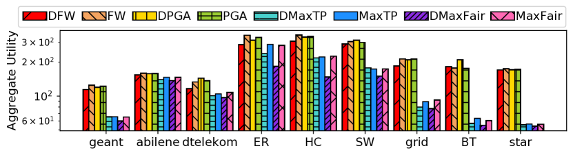
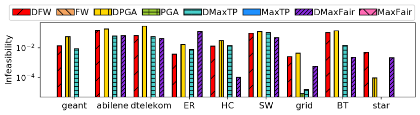
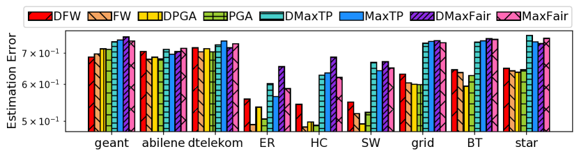
Different Topologies. We first compare the proposed algorithms with several baselines in terms of aggregate utility, infeasibility and estimation error over several network topologies, shown in Fig.ย 2. Our proposed algorithms dramatically outperform all competitors, and our distributed algorithms perform closed to their corresponding centralized algorithms (c.f. Thm.ย 3). All of the distributed algorithms have a low infeasibility, which is less than 0.1. Such violations over the constraints are expected by primal-dual gradient algorithms, since they employ soft constraints.

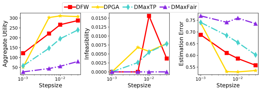
Effect of Stepsizes. We study the effect of the stepsizes in the primal dual gradient algorithms used in the distributed algorithms DFW, DPGA, DMaxTP and DMaxFair over ER, shown in Fig.ย 3. When the algorithms are stable, larger stepsizes achieve better performance w.r.t.ย both aggregate utility and estimation error, while worse performance with respect toย infeasibility. However, if the stepsize is too large, the algorithms do not converge and become numerically unstable. It is crucial to choose an appropriate stepsize for better performance, while maintaining convergence. In all convergent cases, DFW and DPGA outperform competitors.

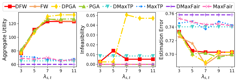
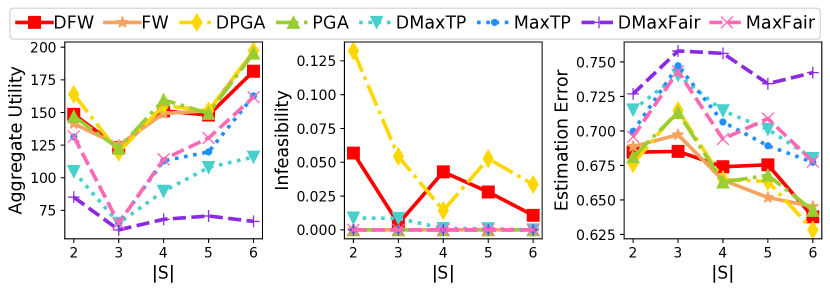
Varying Source Rates and Source Set Size. Next, we evaluate how algorithm performance is affected by varying the (common) source rates ฮปs,tsubscript๐œ†๐‘ ๐‘ก\lambda_{s,t} over topology GEANT. As shown in Fig.ย 4(a), when source rates increase, the aggregate utility first increases very fast and then tapers off. Higher source rates indicate more data received at the learners, hence the greater utility. However, due to DR-submodularity, the marginal gain decreases as the number of sources increases. Furthermore, under limited bandwidth, if link capacities saturate, there will be no further utility increase. The same interpretation applies to the estimation error. We observe similarly changing patterns when varying the source set size $|\mathcal{S}|$ over topology GEANT, shown in Fig.ย 4(b), since more sources also indicates learners receive more data. However, the curve changes are not as smooth as those for increasing the source rates. This is because varying source sets also changes the available paths, corresponding link bandwidth utilization, indexes of well-known features, etc. Overall, we observe that our algorithms, DFW and DPGA, stay close to their centralized versions (FW and PGA) and outperform competitors in both metrics, with a small change in feasibility.

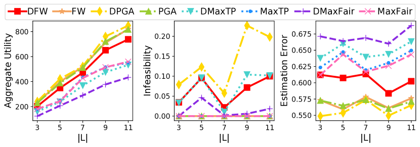
Varying Learner Set Size. Finally, we evaluate the effect of the learner set sizeย |โ„’|โ„’|\mathcal{L}| over topology SW. Fig.ย 5 shows that as the number of learners increases so does the aggregate utility, while the estimation errors essentially remain the same. With multicast transmissions, increasing the number of learners barely affects the amount of data received by each learner. Thus, the aggregate utility increases as expected, while the average utility per learner (the aggregate utility divided by the number of learners) and, consequently, the estimation error hardly change, when more learners are in the network. Again, our algorithms, DFW and DPGA, stay close to their centralized versions (FW and PGA) and outperform competitors.

VIII Conclusion

We generalize the experimental design networks by considering Gaussian sources and multicast transmissions. A poly-time distributed algorithm with $1-1/e$ approximation guarantee is proposed to facilitate heterogeneous model learning across networks. One limitation of our distributed algorithm is its synchronization. It is natural to extend the model to an asynchronous setting, which better resembles the reality of large networks. One possible solution is that sources and links compute outdated gradientsย [6]. Another interesting direction is to estimate gradients through shadow pricesย [33, 34], instead of sampling. Furthermore, how a model trained by one learner benefits other training tasks in experimental design networks is also a worthwhile topic to study. The authors have provided public access to their code and data.222https://github.com/neu-spiral/DistributedNetworkLearning

Acknowledgment

The authors gratefully acknowledge support from the National Science Foundation (grants 1718355, 2106891, 2107062, and 2112471).

References

  • [1] Y.ย Liu, Y.ย Li, L.ย Su, E.ย Yeh, and S.ย Ioannidis, โ€œExperimental design networks: A paradigm for serving heterogeneous learners under networking constraints,โ€ in IEEE INFOCOM 2022.ย ย ย IEEE, 2022, pp. 210โ€“219.
  • [2] M.ย Mohammadi and A.ย Al-Fuqaha, โ€œEnabling cognitive smart cities using big data and machine learning: Approaches and challenges,โ€ IEEE Communications Magazine, vol.ย 56, no.ย 2, pp. 94โ€“101, 2018.
  • [3] V.ย Albino, U.ย Berardi, and R.ย M. Dangelico, โ€œSmart cities: Definitions, dimensions, performance, and initiatives,โ€ Journal of urban technology, vol.ย 22, no.ย 1, pp. 3โ€“21, 2015.
  • [4] A.ย A. Bian, B.ย Mirzasoleiman, J.ย Buhmann, and A.ย Krause, โ€œGuaranteed non-convex optimization: Submodular maximization over continuous domains,โ€ in Artificial Intelligence and Statistics.ย ย ย PMLR, 2017, pp. 111โ€“120.
  • [5] T.ย Soma and Y.ย Yoshida, โ€œA generalization of submodular cover via the diminishing return property on the integer lattice,โ€ Advances in neural information processing systems, vol.ย 28, 2015.
  • [6] S.ย H. Low and D.ย E. Lapsley, โ€œOptimization flow control. i. basic algorithm and convergence,โ€ IEEE/ACM Transactions on networking, vol.ย 7, no.ย 6, pp. 861โ€“874, 1999.
  • [7] R.ย Srikant and T.ย BaลŸar, The mathematics of Internet congestion control.ย ย ย Springer, 2004.
  • [8] D.ย S. Lun, N.ย Ratnakar, R.ย Koetter, M.ย Mรฉdard, E.ย Ahmed, and H.ย Lee, โ€œAchieving minimum-cost multicast: A decentralized approach based on network coding,โ€ in Proceedings IEEE 24th Annual Joint Conference of the IEEE Computer and Communications Societies., vol.ย 3.ย ย ย IEEE, 2005, pp. 1607โ€“1617.
  • [9] D.ย S. Lun, N.ย Ratnakar, M.ย Mรฉdard, R.ย Koetter, D.ย R. Karger, T.ย Ho, E.ย Ahmed, and F.ย Zhao, โ€œMinimum-cost multicast over coded packet networks,โ€ IEEE Transactions on information theory, vol.ย 52, no.ย 6, pp. 2608โ€“2623, 2006.
  • [10] S.ย Boyd, S.ย P. Boyd, and L.ย Vandenberghe, Convex Optimization.ย ย ย Cambridge university press, 2004.
  • [11] F.ย Pukelsheim, Optimal design of experiments.ย ย ย Society for Industrial and Applied Mathematics, 2006.
  • [12] T.ย Horel, S.ย Ioannidis, and S.ย Muthukrishnan, โ€œBudget feasible mechanisms for experimental design,โ€ in Latin American Symposium on Theoretical Informatics.ย ย ย Springer, 2014, pp. 719โ€“730.
  • [13] Y.ย Guo, J.ย Dy, D.ย Erdogmus, J.ย Kalpathy-Cramer, S.ย Ostmo, J.ย P. Campbell, M.ย F. Chiang, and S.ย Ioannidis, โ€œAccelerated experimental design for pairwise comparisons,โ€ in SDM.ย ย ย SIAM, 2019, pp. 432โ€“440.
  • [14] N.ย Gast, S.ย Ioannidis, P.ย Loiseau, and B.ย Roussillon, โ€œLinear regression from strategic data sources,โ€ ACM Transactions on Economics and Computation (TEAC), vol.ย 8, no.ย 2, pp. 1โ€“24, 2020.
  • [15] Y.ย Guo, P.ย Tian, J.ย Kalpathy-Cramer, S.ย Ostmo, J.ย P. Campbell, M.ย F. Chiang, D.ย Erdogmus, J.ย G. Dy, and S.ย Ioannidis, โ€œExperimental design under the bradley-terry model.โ€ in IJCAI, 2018, pp. 2198โ€“2204.
  • [16] X.ย Huan and Y.ย M. Marzouk, โ€œSimulation-based optimal bayesian experimental design for nonlinear systems,โ€ Journal of Computational Physics, vol. 232, no.ย 1, pp. 288โ€“317, 2013.
  • [17] G.ย Calinescu, C.ย Chekuri, M.ย Pal, and J.ย Vondrรกk, โ€œMaximizing a monotone submodular function subject to a matroid constraint,โ€ SIAM Journal on Computing, vol.ย 40, no.ย 6, pp. 1740โ€“1766, 2011.
  • [18] A.ย Krause and D.ย Golovin, โ€œSubmodular function maximization.โ€ 2014.
  • [19] D.ย P. Bertsekas, Nonlinear programming.ย ย ย Athena scientific Belmont, 1999.
  • [20] A.ย Nediฤ‡ and A.ย Ozdaglar, โ€œSubgradient methods for saddle-point problems,โ€ Journal of optimization theory and applications, vol. 142, no.ย 1, pp. 205โ€“228, 2009.
  • [21] S.ย A. Alghunaim and A.ย H. Sayed, โ€œLinear convergence of primalโ€“dual gradient methods and their performance in distributed optimization,โ€ Automatica, vol. 117, p. 109003, 2020.
  • [22] D.ย Feijer and F.ย Paganini, โ€œStability of primalโ€“dual gradient dynamics and applications to network optimization,โ€ Automatica, vol.ย 46, no.ย 12, pp. 1974โ€“1981, 2010.
  • [23] D.ย Bertsekas and J.ย Tsitsiklis, Parallel and distributed computation: numerical methods.ย ย ย Athena Scientific, 2015.
  • [24] G.ย Tychogiorgos, A.ย Gkelias, and K.ย K. Leung, โ€œA non-convex distributed optimization framework and its application to wireless ad-hoc networks,โ€ IEEE Transactions on Wireless Communications, vol.ย 12, no.ย 9, pp. 4286โ€“4296, 2013.
  • [25] A.ย Mokhtari, H.ย Hassani, and A.ย Karbasi, โ€œDecentralized submodular maximization: Bridging discrete and continuous settings,โ€ in International conference on machine learning.ย ย ย PMLR, 2018, pp. 3616โ€“3625.
  • [26] G.ย James, D.ย Witten, T.ย Hastie, and R.ย Tibshirani, An introduction to statistical learning.ย ย ย Springer, 2013, vol. 112.
  • [27] R.ย G. Gallager, Stochastic Processes: Theory for Applications.ย ย ย Cambridge University Press, 2013.
  • [28] F.ย P. Kelly, Reversibility and stochastic networks.ย ย ย Cambridge University Press, 2011.
  • [29] A.ย Rinaldo, โ€œSub-gaussian vectors and bound for the their norm.โ€ 2019. [Online]. Available: https://www.stat.cmu.edu/~arinaldo/Teaching/36709/S19/Scribed_Lectures/Feb21_Shenghao.pdf
  • [30] H.ย Hassani, M.ย Soltanolkotabi, and A.ย Karbasi, โ€œGradient methods for submodular maximization,โ€ in NeurIPS, 2017, pp. 5843โ€“5853.
  • [31] J.ย Kleinberg, โ€œThe small-world phenomenon: An algorithmic perspective,โ€ in STOC, 2000.
  • [32] D.ย Rossi and G.ย Rossini, โ€œCaching performance of content centric networks under multi-path routing (and more),โ€ Telecom ParisTech, Tech. Rep., 2011.
  • [33] S.ย Ioannidis, A.ย Chaintreau, and L.ย Massouliรฉ, โ€œOptimal and scalable distribution of content updates over a mobile social network,โ€ in IEEE INFOCOM 2009.ย ย ย IEEE, 2009, pp. 1422โ€“1430.
  • [34] F.ย P. Kelly, A.ย K. Maulloo, and D.ย K.ย H. Tan, โ€œRate control for communication networks: shadow prices, proportional fairness and stability,โ€ Journal of the Operational Research society, vol.ย 49, no.ย 3, pp. 237โ€“252, 1998.
  • [35] A.ย G. Akritas, E.ย K. Akritas, and G.ย I. Malaschonok, โ€œVarious proofs of sylvesterโ€™s (determinant) identity,โ€ Mathematics and Computers in Simulation, vol.ย 42, no. 4-6, pp. 585โ€“593, 1996.
  • [36] C.ย L. Canonne, โ€œA short note on poisson tail bounds,โ€ 2017. [Online]. Available: http://www.cs.columbia.edu/~ccanonne/files/misc/2017-poissonconcentration.pdf
  • [37] N.ย Alon and J.ย H. Spencer, The probabilistic method.ย ย ย John Wiley & Sons, 2004.
  • [38] R.ย A. Horn and C.ย R. Johnson, Matrix analysis.ย ย ย Cambridge university press, 2012.

Appendix A Proof of Theorem 1

Consider an equivalent data generation process, in which infinite sequences of independent Gaussian variables ๐‘ฟโ„“~=[[๐’™s,iโ„“]i=1โˆž]sโˆˆ๐’ฎ~superscript๐‘ฟโ„“subscriptdelimited-[]superscriptsubscriptdelimited-[]superscriptsubscript๐’™๐‘ ๐‘–โ„“๐‘–1๐‘ ๐’ฎ\widetilde{\boldsymbol{X}^{\ell}}=[[\boldsymbol{x}_{s,i}^{\ell}]_{i=1}^{\infty}]_{s\in\mathcal{S}} from different sources s๐‘ s are received by the learner, but only an initial part of each (as governed by $\boldsymbol{n}^{\ell}$) is observed. Note that the statistics of this process are identical to the actual arrival process, where samples are independent conditioned on $\boldsymbol{n}^{\ell}$. Then, combining the proof of Lem.ย 1 in [1] using Sylvesterโ€™s determinant identity [35, 12] and telescoping sum, we get:

Lemma 2.

Function $G^{\ell}(\widetilde{\boldsymbol{X}^{\ell}},\boldsymbol{n}^{\ell})$ is (a) monotone-increasing and (b) DR-submodular w.r.t. $\boldsymbol{n}^{\ell}$, where ๐—โ„“~=[[๐ฑs,iโ„“]i=1โˆž]sโˆˆ๐’ฎ~superscript๐—โ„“subscriptdelimited-[]superscriptsubscriptdelimited-[]superscriptsubscript๐ฑ๐‘ ๐‘–โ„“๐‘–1๐‘ ๐’ฎ\widetilde{\boldsymbol{X}^{\ell}}=[[\boldsymbol{x}_{s,i}^{\ell}]_{i=1}^{\infty}]_{s\in\mathcal{S}}.

Proof.

For $\boldsymbol{n}\in\mathbb{N}^{|\mathcal{S}|}$, we have:

$\displaystyle G(\boldsymbol{X},\boldsymbol{n}+\boldsymbol{e}_{s^{\prime}}))-G(\boldsymbol{X},\boldsymbol{n})=$ logโ€‹det(โˆ‘sโˆˆ๐’ฎโˆ‘i=1ns๐’™s,iโ€‹๐’™s,iโŠคฯƒs2+๐’™sโ€ฒ,nsโ€ฒ+1โ€‹๐’™sโ€ฒ,nsโ€ฒ+1โŠคฯƒsโ€ฒ2+๐šบ0โˆ’1)โˆ’logโ€‹det(โˆ‘sโˆˆ๐’ฎโˆ‘i=1ns๐’™s,iโ€‹๐’™s,iโŠคฯƒs2+๐šบ0โˆ’1)subscript๐‘ ๐’ฎsuperscriptsubscript๐‘–1subscript๐‘›๐‘ subscript๐’™๐‘ ๐‘–superscriptsubscript๐’™๐‘ ๐‘–topsuperscriptsubscript๐œŽ๐‘ 2subscript๐’™superscript๐‘ โ€ฒsubscript๐‘›superscript๐‘ โ€ฒ1superscriptsubscript๐’™superscript๐‘ โ€ฒsubscript๐‘›superscript๐‘ โ€ฒ1topsuperscriptsubscript๐œŽsuperscript๐‘ โ€ฒ2superscriptsubscript๐šบ01subscript๐‘ ๐’ฎsuperscriptsubscript๐‘–1subscript๐‘›๐‘ subscript๐’™๐‘ ๐‘–superscriptsubscript๐’™๐‘ ๐‘–topsuperscriptsubscript๐œŽ๐‘ 2superscriptsubscript๐šบ01\displaystyle\log\det\big{(}\sum_{s\in\mathcal{S}}\sum_{i=1}^{n_{s}}\frac{\boldsymbol{x}_{s,i}\boldsymbol{x}_{s,i}^{\top}}{\sigma_{s}^{2}}+\frac{\boldsymbol{x}_{s^{\prime},n_{s^{\prime}}+1}\boldsymbol{x}_{s^{\prime},n_{s^{\prime}}+1}^{\top}}{\sigma_{s^{\prime}}^{2}}+\boldsymbol{\Sigma}_{0}^{-1}\big{)}-\log\det\big{(}\sum_{s\in\mathcal{S}}\sum_{i=1}^{n_{s}}\frac{\boldsymbol{x}_{s,i}\boldsymbol{x}_{s,i}^{\top}}{\sigma_{s}^{2}}+\boldsymbol{\Sigma}_{0}^{-1}\big{)}
$\displaystyle=$ logโ€‹det(๐‘ฐd+๐’™sโ€ฒ,nsโ€ฒ+1โ€‹๐’™sโ€ฒ,nsโ€ฒ+1โŠคฯƒsโ€ฒ2โ€‹(โˆ‘sโˆˆ๐’ฎโˆ‘i=1ns๐’™s,iโ€‹๐’™s,iโŠคฯƒs2+๐šบ0โˆ’1)โˆ’1)subscript๐‘ฐ๐‘‘subscript๐’™superscript๐‘ โ€ฒsubscript๐‘›superscript๐‘ โ€ฒ1superscriptsubscript๐’™superscript๐‘ โ€ฒsubscript๐‘›superscript๐‘ โ€ฒ1topsuperscriptsubscript๐œŽsuperscript๐‘ โ€ฒ2superscriptsubscript๐‘ ๐’ฎsuperscriptsubscript๐‘–1subscript๐‘›๐‘ subscript๐’™๐‘ ๐‘–superscriptsubscript๐’™๐‘ ๐‘–topsuperscriptsubscript๐œŽ๐‘ 2superscriptsubscript๐šบ011\displaystyle\log\det\big{(}\boldsymbol{I}_{d}+\frac{\boldsymbol{x}_{s^{\prime},n_{s^{\prime}}+1}\boldsymbol{x}_{s^{\prime},n_{s^{\prime}}+1}^{\top}}{\sigma_{s^{\prime}}^{2}}\big{(}\sum_{s\in\mathcal{S}}\sum_{i=1}^{n_{s}}\frac{\boldsymbol{x}_{s,i}\boldsymbol{x}_{s,i}^{\top}}{\sigma_{s}^{2}}+\boldsymbol{\Sigma}_{0}^{-1}\big{)}^{-1}\big{)}
$\displaystyle=$ logโ€‹det(๐‘ฐ1+1ฯƒsโ€ฒ2โ€‹๐’™sโ€ฒ,nsโ€ฒ+1โŠคโ€‹๐‘จโ€‹(๐’)โ€‹๐’™sโ€ฒ,nsโ€ฒ+1)subscript๐‘ฐ11superscriptsubscript๐œŽsuperscript๐‘ โ€ฒ2superscriptsubscript๐’™superscript๐‘ โ€ฒsubscript๐‘›superscript๐‘ โ€ฒ1top๐‘จ๐’subscript๐’™superscript๐‘ โ€ฒsubscript๐‘›superscript๐‘ โ€ฒ1\displaystyle\log\det\big{(}\boldsymbol{I}_{1}+\frac{1}{\sigma_{s^{\prime}}^{2}}\boldsymbol{x}_{s^{\prime},n_{s^{\prime}}+1}^{\top}\boldsymbol{A}(\boldsymbol{n})\boldsymbol{x}_{s^{\prime},n_{s^{\prime}}+1}\big{)}
$\displaystyle=$ logโก(1+1ฯƒsโ€ฒ2โ€‹๐’™sโ€ฒ,nsโ€ฒ+1โŠคโ€‹๐‘จโ€‹(๐’)โ€‹๐’™sโ€ฒ,nsโ€ฒ+1)11superscriptsubscript๐œŽsuperscript๐‘ โ€ฒ2superscriptsubscript๐’™superscript๐‘ โ€ฒsubscript๐‘›superscript๐‘ โ€ฒ1top๐‘จ๐’subscript๐’™superscript๐‘ โ€ฒsubscript๐‘›superscript๐‘ โ€ฒ1\displaystyle\log\big{(}1+\frac{1}{\sigma_{s^{\prime}}^{2}}\boldsymbol{x}_{s^{\prime},n_{s^{\prime}}+1}^{\top}\boldsymbol{A}(\boldsymbol{n})\boldsymbol{x}_{s^{\prime},n_{s^{\prime}}+1}\big{)}

where ๐‘จโ€‹(๐’)=(โˆ‘sโˆˆ๐’ฎโˆ‘i=1ns๐’™s,iโ€‹๐’™s,iโŠคฯƒs2+๐šบ0โˆ’1)โˆ’1๐‘จ๐’superscriptsubscript๐‘ ๐’ฎsuperscriptsubscript๐‘–1subscript๐‘›๐‘ subscript๐’™๐‘ ๐‘–superscriptsubscript๐’™๐‘ ๐‘–topsuperscriptsubscript๐œŽ๐‘ 2superscriptsubscript๐šบ011\boldsymbol{A}(\boldsymbol{n})=\big{(}\sum_{s\in\mathcal{S}}\sum_{i=1}^{n_{s}}\frac{\boldsymbol{x}_{s,i}\boldsymbol{x}_{s,i}^{\top}}{\sigma_{s}^{2}}+\boldsymbol{\Sigma}_{0}^{-1}\big{)}^{-1} and the second last equality follows Sylvesterโ€™s determinant identity. Then for $\boldsymbol{n}\in\mathbb{N}^{|\mathcal{S}|}$ and $k\in\mathbb{N}$, by telescoping sum, we have

$\displaystyle G(\boldsymbol{X},\boldsymbol{n}+k\boldsymbol{e}_{s^{\prime}}))-G(\boldsymbol{X},\boldsymbol{n})$
$\displaystyle=$ $\displaystyle G(\boldsymbol{X},\boldsymbol{n}+k\boldsymbol{e}_{s^{\prime}}))-G(\boldsymbol{X},\boldsymbol{n}+(k-1)\boldsymbol{e}_{s^{\prime}}))+\cdots+(G(\boldsymbol{X},\boldsymbol{n}+\boldsymbol{e}_{s^{\prime}}))-G(\boldsymbol{X},\boldsymbol{n}))$
$\displaystyle=$ logโก(1+1ฯƒ2โ€‹๐’™sโ€ฒ,nsโ€ฒ+kโŠคโ€‹๐‘จโ€‹(๐’+(kโˆ’1)โ€‹๐’†sโ€ฒ)โ€‹๐’™sโ€ฒ,nsโ€ฒ+k)+โ‹ฏ+logโก(1+1ฯƒ2โ€‹๐’™sโ€ฒ,nsโ€ฒ+1โŠคโ€‹๐‘จโ€‹(๐’)โ€‹๐’™sโ€ฒ,nsโ€ฒ+1)11superscript๐œŽ2superscriptsubscript๐’™superscript๐‘ โ€ฒsubscript๐‘›superscript๐‘ โ€ฒ๐‘˜top๐‘จ๐’๐‘˜1subscript๐’†superscript๐‘ โ€ฒsubscript๐’™superscript๐‘ โ€ฒsubscript๐‘›superscript๐‘ โ€ฒ๐‘˜โ‹ฏ11superscript๐œŽ2superscriptsubscript๐’™superscript๐‘ โ€ฒsubscript๐‘›superscript๐‘ โ€ฒ1top๐‘จ๐’subscript๐’™superscript๐‘ โ€ฒsubscript๐‘›superscript๐‘ โ€ฒ1\displaystyle\log\big{(}1+\frac{1}{\sigma^{2}}\boldsymbol{x}_{s^{\prime},n_{s^{\prime}}+k}^{\top}\boldsymbol{A}(\boldsymbol{n}+(k-1)\boldsymbol{e}_{s^{\prime}})\boldsymbol{x}_{s^{\prime},n_{s^{\prime}}+k}\big{)}+\cdots+\log\big{(}1+\frac{1}{\sigma^{2}}\boldsymbol{x}_{s^{\prime},n_{s^{\prime}}+1}^{\top}\boldsymbol{A}(\boldsymbol{n})\boldsymbol{x}_{s^{\prime},n_{s^{\prime}}+1}\big{)}

where ๐‘จโ€‹(๐’)=(โˆ‘sโˆˆ๐’ฎโˆ‘i=1ns๐’™s,iโ€‹๐’™s,iโŠคฯƒs2+๐šบ0โˆ’1)โˆ’1๐‘จ๐’superscriptsubscript๐‘ ๐’ฎsuperscriptsubscript๐‘–1subscript๐‘›๐‘ subscript๐’™๐‘ ๐‘–superscriptsubscript๐’™๐‘ ๐‘–topsuperscriptsubscript๐œŽ๐‘ 2superscriptsubscript๐šบ011\boldsymbol{A}(\boldsymbol{n})=\big{(}\sum_{s\in\mathcal{S}}\sum_{i=1}^{n_{s}}\frac{\boldsymbol{x}_{s,i}\boldsymbol{x}_{s,i}^{\top}}{\sigma_{s}^{2}}+\boldsymbol{\Sigma}_{0}^{-1}\big{)}^{-1} and the second last equality follows Sylvesterโ€™s determinant identity. The monotonicity of $G$ follows because $A(\boldsymbol{n})$ is positive semidefinite. Finally, since the matrix inverse is decreasing over the positive semi-definite order, we have $A(\boldsymbol{n})\succeq A(\boldsymbol{m})$, $\forall\ \boldsymbol{n},\boldsymbol{m}\in\mathbb{N}^{|\mathcal{S}|},k\in\mathbb{N}\text{ and }\boldsymbol{n}\leq\boldsymbol{m}$, which leads to Gโ€‹(๐‘ฟ,๐’+kโ€‹๐’†s)โˆ’Gโ€‹(๐‘ฟ,๐’)โ‰ฅGโ€‹(๐‘ฟ,๐’Ž+kโ€‹๐’†s)โˆ’Gโ€‹(๐‘ฟ,๐’Ž)๐บ๐‘ฟ๐’๐‘˜subscript๐’†๐‘ ๐บ๐‘ฟ๐’๐บ๐‘ฟ๐’Ž๐‘˜subscript๐’†๐‘ ๐บ๐‘ฟ๐’ŽG(\boldsymbol{X},\boldsymbol{n}+k\boldsymbol{e}_{s})-G(\boldsymbol{X},\boldsymbol{n})\geq G(\boldsymbol{X},\boldsymbol{m}+k\boldsymbol{e}_{s})-G(\boldsymbol{X},\boldsymbol{m}). โˆŽ

Armed with this result, we use a truncation argument to prove that taking expectations w.r.t.ย the (infinite) sequences ๐‘ฟโ„“~=[[๐’™s,iโ„“]i=1โˆž]sโˆˆ๐’ฎ~superscript๐‘ฟโ„“subscriptdelimited-[]superscriptsubscriptdelimited-[]superscriptsubscript๐’™๐‘ ๐‘–โ„“๐‘–1๐‘ ๐’ฎ\widetilde{\boldsymbol{X}^{\ell}}=[[\boldsymbol{x}_{s,i}^{\ell}]_{i=1}^{\infty}]_{s\in\mathcal{S}} preserves submodularity:

Lemma 3.

Function $g^{\ell}(\boldsymbol{n}^{\ell})=\mathbb{E}_{\boldsymbol{X}^{\ell}}[G(\widetilde{\boldsymbol{X}^{\ell}},\boldsymbol{n}^{\ell})|\boldsymbol{n}^{\ell}]$ is (a) monotone-increasing and (b) DR-submodular w.r.t. $\boldsymbol{n}^{\ell}$.

Proof.

Letโ€™s consider a projection:

ฮ n0โ€‹(๐’)=๐’~=[n~s]sโˆˆ๐’ฎ,subscriptฮ subscript๐‘›0๐’~๐’subscriptdelimited-[]subscript~๐‘›๐‘ ๐‘ ๐’ฎ\mathrm{\Pi}_{n_{0}}(\boldsymbol{n})=\tilde{\boldsymbol{n}}=[\tilde{n}_{s}]_{s\in\mathcal{S}},

where

n~s={ns,ย ifย โ€‹nsโ‰คn0n0,ย otherwise.subscript~๐‘›๐‘ casessubscript๐‘›๐‘ ย ifย subscript๐‘›๐‘ subscript๐‘›0otherwisesubscript๐‘›0ย otherwise.otherwise\tilde{n}_{s}=\begin{cases}n_{s},\text{ if }n_{s}\leq n_{0}\\ n_{0},\text{ otherwise.}\end{cases}

Then, consider a function:

Gn0โ€‹(๐‘ฟ~,๐’)=Gโ€‹(๐‘ฟ~,ฮ n0โ€‹(๐’))={Gโ€‹(๐‘ฟ~,๐’),ย ifย โ€‹โ€–๐’โ€–โˆžโ‰คn0Gโ€‹(๐‘ฟ~,ฮ n0โ€‹(๐’)),ย otherwise.subscript๐บsubscript๐‘›0~๐‘ฟ๐’๐บ~๐‘ฟsubscriptฮ subscript๐‘›0๐’cases๐บ~๐‘ฟ๐’ย ifย subscriptnorm๐’subscript๐‘›0otherwise๐บ~๐‘ฟsubscriptฮ subscript๐‘›0๐’ย otherwise.otherwiseG_{n_{0}}(\widetilde{\boldsymbol{X}},\boldsymbol{n})=G(\widetilde{\boldsymbol{X}},\mathrm{\Pi}_{n_{0}}(\boldsymbol{n}))=\begin{cases}G(\widetilde{\boldsymbol{X}},\boldsymbol{n}),\text{ if }\|\boldsymbol{n}\|_{\infty}\leq n_{0}\\ G(\widetilde{\boldsymbol{X}},\mathrm{\Pi}_{n_{0}}(\boldsymbol{n})),\text{ otherwise.}\end{cases}

It is easy to verify that $\forall\ \boldsymbol{n},\boldsymbol{m}\in\mathbb{N}^{|\mathcal{S}|}\ \text{and}\ \boldsymbol{n}\leq\boldsymbol{m}$, we have Gn0โ€‹(๐‘ฟ~,๐’+kโ€‹๐’†s)โˆ’Gn0โ€‹(๐‘ฟ~,๐’)โ‰ฅGn0โ€‹(๐‘ฟ~,๐’Ž+kโ€‹๐’†s)โˆ’Gn0โ€‹(๐‘ฟ~,๐’Ž)subscript๐บsubscript๐‘›0~๐‘ฟ๐’๐‘˜subscript๐’†๐‘ subscript๐บsubscript๐‘›0~๐‘ฟ๐’subscript๐บsubscript๐‘›0~๐‘ฟ๐’Ž๐‘˜subscript๐’†๐‘ subscript๐บsubscript๐‘›0~๐‘ฟ๐’ŽG_{n_{0}}(\widetilde{\boldsymbol{X}},\boldsymbol{n}+k\boldsymbol{e}_{s})-G_{n_{0}}(\widetilde{\boldsymbol{X}},\boldsymbol{n})\geq G_{n_{0}}(\widetilde{\boldsymbol{X}},\boldsymbol{m}+k\boldsymbol{e}_{s})-G_{n_{0}}(\widetilde{\boldsymbol{X}},\boldsymbol{m}). Thus, $G_{n_{0}}(\widetilde{\boldsymbol{X}},\boldsymbol{n})$ is DR-submodular w.r.t. $\boldsymbol{n}$.

Consider $g_{n_{0}}(\boldsymbol{n})=\mathbb{E}_{\widetilde{\boldsymbol{X}}}[G_{n_{0}}(\widetilde{\boldsymbol{X}},\boldsymbol{n})|\boldsymbol{n}]$. As an expectation of โ€™finite $\widetilde{\boldsymbol{X}}$โ€™, $g_{n_{0}}(\boldsymbol{n})$ is still DR-submodular, i.e., $\forall\ \boldsymbol{n},\boldsymbol{m}\in\mathbb{N}^{|\mathcal{S}|},\ \boldsymbol{n}\leq\boldsymbol{m}\ \text{and}\ \forall\ n_{0}\in\mathbb{N}$, we have gn0โ€‹(๐’+kโ€‹๐’†s)โˆ’gn0โ€‹(๐’)โ‰ฅgn0โ€‹(๐’Ž+kโ€‹๐’†s)โˆ’gn0โ€‹(๐’Ž)subscript๐‘”subscript๐‘›0๐’๐‘˜subscript๐’†๐‘ subscript๐‘”subscript๐‘›0๐’subscript๐‘”subscript๐‘›0๐’Ž๐‘˜subscript๐’†๐‘ subscript๐‘”subscript๐‘›0๐’Žg_{n_{0}}(\boldsymbol{n}+k\boldsymbol{e}_{s})-g_{n_{0}}(\boldsymbol{n})\geq g_{n_{0}}(\boldsymbol{m}+k\boldsymbol{e}_{s})-g_{n_{0}}(\boldsymbol{m}). Observe that $\lim_{n_{0}\to\infty}g_{n_{0}}(\boldsymbol{n})=g(\boldsymbol{n})$, $\forall\ \boldsymbol{n}^{\prime}\in\mathbb{N}^{|\mathcal{S}|}$. In fact, $\forall\ \boldsymbol{n}^{\prime}\in\mathbb{N}^{|\mathcal{S}|}$, $\exists\ n_{0}(\boldsymbol{n}^{\prime})=\|\boldsymbol{n}^{\prime}\|_{\infty}$, s.t. $g_{n_{0}}(\boldsymbol{n}^{\prime})=g(\boldsymbol{n}^{\prime})$. Furthermore, โˆƒn0=maxโก{โ€–๐’โ€–โˆž,โ€–๐’+kโ€‹๐’†sโ€–โˆž,โ€–๐’Žโ€–โˆž,โ€–๐’Ž+kโ€‹๐’†sโ€–โˆž}subscript๐‘›0subscriptnorm๐’subscriptnorm๐’๐‘˜subscript๐’†๐‘ subscriptnorm๐’Žsubscriptnorm๐’Ž๐‘˜subscript๐’†๐‘ \exists n_{0}=\max\{\|\boldsymbol{n}\|_{\infty},\|\boldsymbol{n}+k\boldsymbol{e}_{s}\|_{\infty},\|\boldsymbol{m}\|_{\infty},\|\boldsymbol{m}+k\boldsymbol{e}_{s}\|_{\infty}\}, s.t. $g_{n_{0}}(\boldsymbol{n})=g(\boldsymbol{n})$, gn0โ€‹(๐’+kโ€‹๐’†s)=gโ€‹(๐’+kโ€‹๐’†s)subscript๐‘”subscript๐‘›0๐’๐‘˜subscript๐’†๐‘ ๐‘”๐’๐‘˜subscript๐’†๐‘ g_{n_{0}}(\boldsymbol{n}+k\boldsymbol{e}_{s})=g(\boldsymbol{n}+k\boldsymbol{e}_{s}), $g_{n_{0}}(\boldsymbol{m})=g(\boldsymbol{m})$, gn0โ€‹(๐’Ž+kโ€‹๐’†s)=gโ€‹(๐’Ž+kโ€‹๐’†s)subscript๐‘”subscript๐‘›0๐’Ž๐‘˜subscript๐’†๐‘ ๐‘”๐’Ž๐‘˜subscript๐’†๐‘ g_{n_{0}}(\boldsymbol{m}+k\boldsymbol{e}_{s})=g(\boldsymbol{m}+k\boldsymbol{e}_{s}), and gโ€‹(๐’+kโ€‹๐’†s)โˆ’gโ€‹(๐’)โ‰ฅgโ€‹(๐’Ž+kโ€‹๐’†s)โˆ’gโ€‹(๐’Ž)๐‘”๐’๐‘˜subscript๐’†๐‘ ๐‘”๐’๐‘”๐’Ž๐‘˜subscript๐’†๐‘ ๐‘”๐’Žg(\boldsymbol{n}+k\boldsymbol{e}_{s})-g(\boldsymbol{n})\geq g(\boldsymbol{m}+k\boldsymbol{e}_{s})-g(\boldsymbol{m}).

Similarly, we could obtain the monotonicity. โˆŽ

Then, we establish the positivity of the gradient and non-positivity of the Hessian of $U$, following Thm.ย 1 in [1] and utilizing Lem.ย 3 to prove our Thm.ย 1.

Proof.

By the law of total expectation:

Uโ„“โ€‹(๐€โ„“)=๐”ผโ€‹[gโ„“โ€‹(๐’โ„“)]=โˆ‘t=0โˆž๐”ผโ€‹[gโ€‹(๐’)|nsโ„“=t]โ‹…(ฮปsโ„“โ€‹T)tโ€‹eโˆ’ฮปsโ„“โ€‹Tt!.superscript๐‘ˆโ„“superscript๐€โ„“๐”ผdelimited-[]superscript๐‘”โ„“superscript๐’โ„“superscriptsubscript๐‘ก0โ‹…๐”ผdelimited-[]conditional๐‘”๐’superscriptsubscript๐‘›๐‘ โ„“๐‘กsuperscriptsuperscriptsubscript๐œ†๐‘ โ„“๐‘‡๐‘กsuperscript๐‘’superscriptsubscript๐œ†๐‘ โ„“๐‘‡๐‘กU^{\ell}(\boldsymbol{\lambda}^{\ell})=\mathbb{E}[g^{\ell}(\boldsymbol{n}^{\ell})]=\sum_{t=0}^{\infty}\mathbb{E}\left[g(\boldsymbol{n})|n_{s}^{\ell}=t\right]\cdot\frac{(\lambda_{s}^{\ell}T)^{t}e^{-\lambda_{s}^{\ell}T}}{t!}.

Thus the first partial derivatives are:

โˆ‚Uโˆ‚ฮปs,tp=๐‘ˆsuperscriptsubscript๐œ†๐‘ ๐‘ก๐‘absent\displaystyle\frac{\partial U}{\partial\lambda_{s,t}^{p}}= โˆ‚Uโ„“โˆ‚ฮปs,tp=โˆ‘t=0โˆž๐”ผโ€‹[gโ€‹(๐’)|nsโ„“=t]โ‹…(tฮปsโ„“โˆ’T)โ€‹(ฮปsโ„“โ€‹T)tโ€‹eโˆ’ฮปsโ„“โ€‹Tt!superscript๐‘ˆโ„“superscriptsubscript๐œ†๐‘ ๐‘ก๐‘superscriptsubscript๐‘ก0โ‹…๐”ผdelimited-[]conditional๐‘”๐’superscriptsubscript๐‘›๐‘ โ„“๐‘ก๐‘กsuperscriptsubscript๐œ†๐‘ โ„“๐‘‡superscriptsuperscriptsubscript๐œ†๐‘ โ„“๐‘‡๐‘กsuperscript๐‘’superscriptsubscript๐œ†๐‘ โ„“๐‘‡๐‘ก\displaystyle\frac{\partial U^{\ell}}{\partial\lambda_{s,t}^{p}}=\sum_{t=0}^{\infty}\mathbb{E}\left[g(\boldsymbol{n})|n_{s}^{\ell}=t\right]\cdot(\frac{t}{\lambda_{s}^{\ell}}-T)\frac{(\lambda_{s}^{\ell}T)^{t}e^{-\lambda_{s}^{\ell}T}}{t!}
$\displaystyle=$ โˆ‘t=0โˆž(๐”ผโ€‹[gโ€‹(๐’)|nsโ„“=t+1]โˆ’๐”ผโ€‹[gโ€‹(๐’)|nsโ„“=t])โ‹…(ฮปsโ„“)tโ€‹Tt+1t!โ€‹eโˆ’ฮปsโ„“โ€‹Tโ‰ฅ0superscriptsubscript๐‘ก0โ‹…๐”ผdelimited-[]conditional๐‘”๐’superscriptsubscript๐‘›๐‘ โ„“๐‘ก1๐”ผdelimited-[]conditional๐‘”๐’superscriptsubscript๐‘›๐‘ โ„“๐‘กsuperscriptsuperscriptsubscript๐œ†๐‘ โ„“๐‘กsuperscript๐‘‡๐‘ก1๐‘กsuperscript๐‘’superscriptsubscript๐œ†๐‘ โ„“๐‘‡0\displaystyle\sum_{t=0}^{\infty}(\mathbb{E}\left[g(\boldsymbol{n})|n_{s}^{\ell}=t+1\right]-\mathbb{E}\left[g(\boldsymbol{n})|n_{s}^{\ell}=t\right])\cdot\frac{(\lambda_{s}^{\ell})^{t}T^{t+1}}{t!}e^{-\lambda_{s}^{\ell}T}\geq 0

by monotonicity of $g$. Note that, here $t=t^{\ell}$ and $\ell=p[-1]$. Next, we compute the second partial derivatives โˆ‚2Uโˆ‚ฮปs,tpโ€‹โˆ‚ฮปsโ€ฒ,tโ€ฒpโ€ฒsuperscript2๐‘ˆsuperscriptsubscript๐œ†๐‘ ๐‘ก๐‘superscriptsubscript๐œ†superscript๐‘ โ€ฒsuperscript๐‘กโ€ฒsuperscript๐‘โ€ฒ\frac{\partial^{2}U}{\partial\lambda_{s,t}^{p}\partial\lambda_{s^{\prime},t^{\prime}}^{p^{\prime}}}. It is easy to see that for โ„“โ‰ โ„“โ€ฒโ„“superscriptโ„“โ€ฒ\ell\neq\ell^{\prime}, we have:

โˆ‚2Uโˆ‚ฮปs,tpโ€‹โˆ‚ฮปsโ€ฒ,tโ€ฒpโ€ฒ=0.superscript2๐‘ˆsuperscriptsubscript๐œ†๐‘ ๐‘ก๐‘superscriptsubscript๐œ†superscript๐‘ โ€ฒsuperscript๐‘กโ€ฒsuperscript๐‘โ€ฒ0\frac{\partial^{2}U}{\partial\lambda_{s,t}^{p}\partial\lambda_{s^{\prime},t^{\prime}}^{p^{\prime}}}=0.

For $\ell=\ell^{\prime}$, which also implies $t=t^{\prime}$, and s=sโ€ฒ๐‘ superscript๐‘ โ€ฒs=s^{\prime}. No matter $p$ equals to $p^{\prime}$ or not, it holds that

โˆ‚2Uโˆ‚ฮปs,tpโ€‹โˆ‚ฮปs,tpโ€ฒ=โˆ‚2Uโ„“โˆ‚(ฮปs,tp)2superscript2๐‘ˆsuperscriptsubscript๐œ†๐‘ ๐‘ก๐‘superscriptsubscript๐œ†๐‘ ๐‘กsuperscript๐‘โ€ฒsuperscript2superscript๐‘ˆโ„“superscriptsuperscriptsubscript๐œ†๐‘ ๐‘ก๐‘2\displaystyle\frac{\partial^{2}U}{\partial\lambda_{s,t}^{p}\partial\lambda_{s,t}^{p^{\prime}}}=\frac{\partial^{2}U^{\ell}}{\partial(\lambda_{s,t}^{p})^{2}}
$\displaystyle=$ (๐”ผโ€‹[gโ€‹(๐’)|nsโ„“=1]โˆ’๐”ผโ€‹[gโ€‹(๐’)|nsโ„“=0])โ‹…(โˆ’T2)โ€‹eโˆ’ฮปsโ„“โ€‹T+โˆ‘t=1โˆž(๐”ผโ€‹[gโ€‹(๐’)|nsโ„“=t+1]โˆ’๐”ผโ€‹[gโ€‹(๐’)|nsโ„“=t])โ‹…โ€ฆโ‹…๐”ผdelimited-[]conditional๐‘”๐’superscriptsubscript๐‘›๐‘ โ„“1๐”ผdelimited-[]conditional๐‘”๐’superscriptsubscript๐‘›๐‘ โ„“0superscript๐‘‡2superscript๐‘’superscriptsubscript๐œ†๐‘ โ„“๐‘‡superscriptsubscript๐‘ก1โ‹…๐”ผdelimited-[]conditional๐‘”๐’superscriptsubscript๐‘›๐‘ โ„“๐‘ก1๐”ผdelimited-[]conditional๐‘”๐’superscriptsubscript๐‘›๐‘ โ„“๐‘กโ€ฆ\displaystyle(\mathbb{E}\left[g(\boldsymbol{n})|n_{s}^{\ell}=1\right]-\mathbb{E}\left[g(\boldsymbol{n})|n_{s}^{\ell}=0\right])\cdot(-T^{2})e^{-\lambda_{s}^{\ell}T}+\sum_{t=1}^{\infty}(\mathbb{E}\left[g(\boldsymbol{n})|n_{s}^{\ell}=t+1\right]-\mathbb{E}\left[g(\boldsymbol{n})|n_{s}^{\ell}=t\right])\cdot\ldots
((ฮปsโ„“)tโˆ’1โ€‹Tt+1(tโˆ’1)!โˆ’(ฮปsโ„“)tโ€‹Tt+2t!)โ€‹eโˆ’ฮปsโ„“โ€‹Tsuperscriptsuperscriptsubscript๐œ†๐‘ โ„“๐‘ก1superscript๐‘‡๐‘ก1๐‘ก1superscriptsuperscriptsubscript๐œ†๐‘ โ„“๐‘กsuperscript๐‘‡๐‘ก2๐‘กsuperscript๐‘’superscriptsubscript๐œ†๐‘ โ„“๐‘‡\displaystyle\quad(\frac{(\lambda_{s}^{\ell})^{t-1}T^{t+1}}{(t-1)!}-\frac{(\lambda_{s}^{\ell})^{t}T^{t+2}}{t!})e^{-\lambda_{s}^{\ell}T}
$\displaystyle=$ โˆ‘t=1โˆž((๐”ผโ€‹[gโ€‹(๐’)|nsโ„“=t+1]โˆ’๐”ผโ€‹[gโ€‹(๐’)|nsโ„“=t])โˆ’(๐”ผโ€‹[gโ€‹(๐’)|nsโ„“=t]โˆ’๐”ผโ€‹[gโ€‹(๐’)|nsโ„“=tโˆ’1]))โ‹…(ฮปsโ„“)tโˆ’1โ€‹Tt+1(tโˆ’1)!โ€‹eโˆ’ฮปsโ„“โ€‹Tsuperscriptsubscript๐‘ก1โ‹…๐”ผdelimited-[]conditional๐‘”๐’superscriptsubscript๐‘›๐‘ โ„“๐‘ก1๐”ผdelimited-[]conditional๐‘”๐’superscriptsubscript๐‘›๐‘ โ„“๐‘ก๐”ผdelimited-[]conditional๐‘”๐’superscriptsubscript๐‘›๐‘ โ„“๐‘ก๐”ผdelimited-[]conditional๐‘”๐’superscriptsubscript๐‘›๐‘ โ„“๐‘ก1superscriptsuperscriptsubscript๐œ†๐‘ โ„“๐‘ก1superscript๐‘‡๐‘ก1๐‘ก1superscript๐‘’superscriptsubscript๐œ†๐‘ โ„“๐‘‡\displaystyle\sum_{t=1}^{\infty}\left((\mathbb{E}\left[g(\boldsymbol{n})|n_{s}^{\ell}=t+1\right]-\mathbb{E}\left[g(\boldsymbol{n})|n_{s}^{\ell}=t\right])-(\mathbb{E}\left[g(\boldsymbol{n})|\right.\right.\left.\left.n_{s}^{\ell}=t\right]-\mathbb{E}\left[g(\boldsymbol{n})|n_{s}^{\ell}=t-1\right])\right)\cdot\frac{(\lambda_{s}^{\ell})^{t-1}T^{t+1}}{(t-1)!}e^{-\lambda_{s}^{\ell}T}
$\displaystyle\leq$ $\displaystyle 0,$

by the submodularity of $G$. For sโ‰ sโ€ฒ๐‘ superscript๐‘ โ€ฒs\neq s^{\prime}, which also implies pโ‰ pโ€ฒ๐‘superscript๐‘โ€ฒp\neq p^{\prime}

โˆ‚2Uโˆ‚ฮปs,tpโ€‹โˆ‚ฮปsโ€ฒ,tpโ€ฒ=superscript2๐‘ˆsuperscriptsubscript๐œ†๐‘ ๐‘ก๐‘superscriptsubscript๐œ†superscript๐‘ โ€ฒ๐‘กsuperscript๐‘โ€ฒabsent\displaystyle\frac{\partial^{2}U}{\partial\lambda_{s,t}^{p}\partial\lambda_{s^{\prime},t}^{p^{\prime}}}= โˆ‚2Uโ„“โˆ‚ฮปs,tpโ€‹โˆ‚ฮปsโ€ฒ,tpโ€ฒ=โˆ‘t=0โˆžโˆ‘k=0โˆž๐”ผโ€‹[gโ€‹(๐’)|nsโ„“=t,nsโ€ฒโ„“=k]โ‹…โˆ‚โˆ‚ฮปsโ„“โ€‹Pโ€‹(nsโ„“=t)โ‹…โˆ‚โˆ‚ฮปsโ€ฒโ„“โ€‹Pโ€‹(nsโ€ฒโ„“=k)superscript2superscript๐‘ˆโ„“superscriptsubscript๐œ†๐‘ ๐‘ก๐‘superscriptsubscript๐œ†superscript๐‘ โ€ฒ๐‘กsuperscript๐‘โ€ฒsuperscriptsubscript๐‘ก0superscriptsubscript๐‘˜0โ‹…โ‹…๐”ผdelimited-[]formulae-sequenceconditional๐‘”๐’superscriptsubscript๐‘›๐‘ โ„“๐‘กsuperscriptsubscript๐‘›superscript๐‘ โ€ฒโ„“๐‘˜superscriptsubscript๐œ†๐‘ โ„“Psuperscriptsubscript๐‘›๐‘ โ„“๐‘กsuperscriptsubscript๐œ†superscript๐‘ โ€ฒโ„“Psuperscriptsubscript๐‘›superscript๐‘ โ€ฒโ„“๐‘˜\displaystyle\frac{\partial^{2}U^{\ell}}{\partial\lambda_{s,t}^{p}\partial\lambda_{s^{\prime},t}^{p^{\prime}}}=\sum_{t=0}^{\infty}\sum_{k=0}^{\infty}\mathbb{E}\left[g(\boldsymbol{n})|n_{s}^{\ell}=t,n_{s^{\prime}}^{\ell}=k\right]\cdot\frac{\partial}{\partial\lambda_{s}^{\ell}}\mathrm{P}(n_{s}^{\ell}=t)\cdot\frac{\partial}{\partial\lambda_{s^{\prime}}^{\ell}}\mathrm{P}(n_{s^{\prime}}^{\ell}=k)
$\displaystyle=$ $\displaystyle\sum_{t=0}^{\infty}\sum_{k=0}^{\infty}((\mathbb{E}\left[g(\boldsymbol{n})|n_{s}^{\ell}=t+1,n_{s^{\prime}}^{\ell}=k+1\right]-\mathbb{E}\left[g(\boldsymbol{n})|n_{s}^{\ell}=t,n_{s^{\prime}}^{\ell}=k+1\right])-\ldots$
$\displaystyle\quad(\mathbb{E}\left[g(\boldsymbol{n})|n_{s}^{\ell}=t+1,\right.\left.n_{s^{\prime}}^{\ell}=k\right]-\mathbb{E}\left[g(\boldsymbol{n})|n_{s}^{\ell}=t,n_{s^{\prime}}^{\ell}=k\right]))\cdot\frac{(\lambda_{s}^{\ell})^{t}(\lambda_{s^{\prime}}^{\ell})^{k}T^{t+k+2}}{t!k!}e^{-(\lambda_{s}^{\ell}+\lambda_{s^{\prime}}^{\ell})T}$
$\displaystyle\leq$ $\displaystyle 0$

also by the submodularity of $g$. โˆŽ

Appendix B Proof of Lemma 1

We know that Poisson has a subexponential tail boundย [36], then, after truncating, the $\mathrm{HEAD}$, defined in Eq. (16) is guaranteed to be within a constant factor from the true partial derivative:

Lemma 4 (Lemma 4 in [1]).

For $h(u)=2\frac{(1+u)\ln{(1+u)}-u}{u^{2}}$ and nโ€ฒโ‰ฅฮปsโ„“โ€‹Tsuperscript๐‘›โ€ฒsuperscriptsubscript๐œ†๐‘ โ„“๐‘‡n^{\prime}\geq\lambda_{s}^{\ell}T, we have:

โˆ‚Uโˆ‚ฮปs,tpโ‰ฅHEADs,tpโ€‹(nโ€ฒ)โ‰ฅ(1โˆ’๐โ€‹[nsโ„“โ‰ฅnโ€ฒ+1])โ€‹โˆ‚Uโˆ‚ฮปs,tp.๐‘ˆsuperscriptsubscript๐œ†๐‘ ๐‘ก๐‘superscriptsubscriptHEAD๐‘ ๐‘ก๐‘superscript๐‘›โ€ฒ1๐delimited-[]subscriptsuperscript๐‘›โ„“๐‘ superscript๐‘›โ€ฒ1๐‘ˆsuperscriptsubscript๐œ†๐‘ ๐‘ก๐‘\frac{\partial U}{\partial\lambda_{s,t}^{p}}\geq\mathrm{HEAD}_{s,t}^{p}(n^{\prime})\geq(1-\mathbf{P}[n^{\ell}_{s}\geq n^{\prime}+1])\frac{\partial U}{\partial\lambda_{s,t}^{p}}.

To quantify the distance between the estimated gradient and $\mathrm{HEAD}$, we first introduce two auxiliary lemmas as follows. By Chernoff bounds described by Thmย A.1.16 in [37], we get:

Lemma 5.

If there exists a constant vector ๐œ=[cs]sโˆˆ๐’ฎโˆˆโ„|๐’ฎ|๐œsubscriptdelimited-[]subscript๐‘๐‘ ๐‘ ๐’ฎsuperscriptโ„๐’ฎ\boldsymbol{c}=[c_{s}]_{s\in\mathcal{S}}\in\mathbb{R}^{|\mathcal{S}|}, such that for any sโˆˆ๐’ฎ๐‘ ๐’ฎs\in\mathcal{S} and iโ‰คnsโ„“๐‘–superscriptsubscript๐‘›๐‘ โ„“i\leq n_{s}^{\ell}, โ€–๐ฑs,iโ„“โ€–2โ‰คcssubscriptnormsubscriptsuperscript๐ฑโ„“๐‘ ๐‘–2subscript๐‘๐‘ \|\boldsymbol{x}^{\ell}_{s,i}\|_{2}\leq c_{s}, then:

|โˆ‚Uโˆ‚ฮปs,tp^โˆ’HEADs,tp|โ‰คฮณโ€‹maxโ„“โˆˆโ„’,sโˆˆ๐’ฎโกlogโก(1+ฮปMAXโ€‹(๐šบ0โ„“)โ€‹cs2ฯƒs,t2),^๐‘ˆsuperscriptsubscript๐œ†๐‘ ๐‘ก๐‘superscriptsubscriptHEAD๐‘ ๐‘ก๐‘๐›พsubscriptformulae-sequenceโ„“โ„’๐‘ ๐’ฎ1subscript๐œ†MAXsuperscriptsubscript๐šบ0โ„“superscriptsubscript๐‘๐‘ 2superscriptsubscript๐œŽ๐‘ ๐‘ก2\left|\widehat{\frac{\partial U}{\partial\lambda_{s,t}^{p}}}-\mathrm{HEAD}_{s,t}^{p}\right|\leq\gamma\max_{\ell\in\mathcal{L},s\in\mathcal{S}}\log(1+\frac{\lambda_{\mathrm{MAX}}(\boldsymbol{\Sigma}_{0}^{\ell})c_{s}^{2}}{\sigma_{s,t}^{2}}),

with probability greater than $1-2\cdot e^{-\gamma^{2}N_{1}N_{2}/2T^{2}(n^{\prime}+1)}$, where $\lambda_{\mathrm{MAX}}(\boldsymbol{\Sigma}_{0}^{\ell})$ is the maximum eigenvalue of matrix $\boldsymbol{\Sigma}_{0}^{\ell}$.

Proof.

We define

$\displaystyle X^{j,k}(n)=$ Gโ„“โ€‹(๐‘ฟโ„“,j,k,๐’โ„“,j|nsโ„“,j=n+1)โˆ’Gโ„“โ€‹(๐‘ฟโ„“,j,k,๐’โ„“,j|nsโ„“,j=n)โˆ’ฮ”sโ„“โ€‹(๐€โ„“,n)GMAX,superscript๐บโ„“superscript๐‘ฟโ„“๐‘—๐‘˜evaluated-atsuperscript๐’โ„“๐‘—superscriptsubscript๐‘›๐‘ โ„“๐‘—๐‘›1superscript๐บโ„“superscript๐‘ฟโ„“๐‘—๐‘˜evaluated-atsuperscript๐’โ„“๐‘—superscriptsubscript๐‘›๐‘ โ„“๐‘—๐‘›superscriptsubscriptฮ”๐‘ โ„“superscript๐€โ„“๐‘›subscript๐บMAX\displaystyle\frac{G^{\ell}(\boldsymbol{X}^{\ell,j,k},\boldsymbol{n}^{\ell,j}|_{n_{s}^{\ell,j}=n+1})-G^{\ell}(\boldsymbol{X}^{\ell,j,k},\boldsymbol{n}^{\ell,j}|_{n_{s}^{\ell,j}=n})-\Delta_{s}^{\ell}(\boldsymbol{\lambda}^{\ell},n)}{G_{\mathrm{MAX}}},

where GMAX=maxโ„“โˆˆโ„’,sโˆˆ๐’ฎ,๐’™โˆˆBโ€‹(๐ŸŽ;c)โก(Gโ„“โ€‹(๐’™,๐’†s)โˆ’Gโ„“โ€‹(๐’™,๐ŸŽ))=maxโ„“โˆˆโ„’,sโˆˆ๐’ฎ,๐’™โˆˆBโ€‹(๐ŸŽ;c)โกlogโก(1+1ฯƒs,t2โ€‹๐’™sโŠคโ€‹๐šบโ„“โ€‹๐’™s)subscript๐บMAXsubscriptformulae-sequenceโ„“โ„’formulae-sequence๐‘ ๐’ฎ๐’™๐ต0๐‘superscript๐บโ„“๐’™subscript๐’†๐‘ superscript๐บโ„“๐’™0subscriptformulae-sequenceโ„“โ„’formulae-sequence๐‘ ๐’ฎ๐’™๐ต0๐‘11superscriptsubscript๐œŽ๐‘ ๐‘ก2superscriptsubscript๐’™๐‘ topsubscript๐šบbold-โ„“subscript๐’™๐‘ G_{\mathrm{MAX}}=\max_{\ell\in\mathcal{L},s\in\mathcal{S},\boldsymbol{x}\in B(\boldsymbol{0};c)}(G^{\ell}(\boldsymbol{x},\boldsymbol{e}_{s})-G^{\ell}(\boldsymbol{x},\boldsymbol{0}))=\max_{\ell\in\mathcal{L},s\in\mathcal{S},\boldsymbol{x}\in B(\boldsymbol{0};c)}\log\big{(}1+\frac{1}{\sigma_{s,t}^{2}}\boldsymbol{x}_{s}^{\top}\boldsymbol{\Sigma_{\ell}}\boldsymbol{x}_{s}\big{)}. We have $|X^{j,k}(n)|\leq 1$, because:

$\displaystyle G_{\mathrm{MAX}}$ โ‰ฅ(Gโ„“โ€‹(๐’™,๐’†s)โˆ’Gโ„“โ€‹(๐’™,๐ŸŽ))โ‰ฅGโ€‹(๐‘ฟโ„“,j,k,๐’j|nsโ„“,j=n+1)โˆ’Gโ€‹(๐‘ฟโ„“,j,k,๐’j|nsโ„“,j=n),absentsuperscript๐บโ„“๐’™subscript๐’†๐‘ superscript๐บโ„“๐’™0๐บsuperscript๐‘ฟโ„“๐‘—๐‘˜evaluated-atsuperscript๐’๐‘—superscriptsubscript๐‘›๐‘ โ„“๐‘—๐‘›1๐บsuperscript๐‘ฟโ„“๐‘—๐‘˜evaluated-atsuperscript๐’๐‘—superscriptsubscript๐‘›๐‘ โ„“๐‘—๐‘›\displaystyle\geq(G^{\ell}(\boldsymbol{x},\boldsymbol{e}_{s})-G^{\ell}(\boldsymbol{x},\boldsymbol{0}))\geq G(\boldsymbol{X}^{\ell,j,k},\boldsymbol{n}^{j}|_{n_{s}^{\ell,j}=n+1})-G(\boldsymbol{X}^{\ell,j,k},\boldsymbol{n}^{j}|_{n_{s}^{\ell,j}=n}),

for any $\ell\in\mathcal{L}$, sโˆˆ๐’ฎ๐‘ ๐’ฎs\in\mathcal{S}, $\boldsymbol{x}\in B(\boldsymbol{0};c)$, $n\geq 0$. By Chernoff bounds described by Theorem A.1.16 in [37], we have

$$\mathbf{P}\left[\left|\sum_{j=1}^{N_{1}}\sum_{k=1}^{N_{2}}\sum_{n=0}^{n=n^{\prime}}X^{j,k}(n)\right|>c\right]\leq 2e^{-c^{2}/2N_{1}N_{2}(n^{{}^{\prime}}+1)}.$$

Suppose we let $c=\gamma\cdot N_{1}N_{2}/T$, where $\gamma$ is the step size, then we have

|โˆ‚Uโˆ‚ฮปs,tp^โˆ’HEADs,tp|โ‰ค^๐‘ˆsuperscriptsubscript๐œ†๐‘ ๐‘ก๐‘superscriptsubscriptHEAD๐‘ ๐‘ก๐‘absent\displaystyle\left|\widehat{\frac{\partial U}{\partial\lambda_{s,t}^{p}}}-\mathrm{HEAD}_{s,t}^{p}\right|\leq |โˆ‘n=0nโ€ฒโˆ‘j=1N1โˆ‘k=1N2Gโ„“โ€‹(๐‘ฟโ„“,j,k,๐’โ„“,j|nsโ„“,j=n+1)โˆ’Gโ„“โ€‹(๐‘ฟโ„“,j,k,๐’โ„“,j|nsโ„“,j=n)โˆ’ฮ”sโ„“โ€‹(๐€โ„“,n)N1โ€‹N2โ€‹T|superscriptsubscript๐‘›0superscript๐‘›โ€ฒsuperscriptsubscript๐‘—1subscript๐‘1superscriptsubscript๐‘˜1subscript๐‘2superscript๐บโ„“superscript๐‘ฟโ„“๐‘—๐‘˜evaluated-atsuperscript๐’โ„“๐‘—superscriptsubscript๐‘›๐‘ โ„“๐‘—๐‘›1superscript๐บโ„“superscript๐‘ฟโ„“๐‘—๐‘˜evaluated-atsuperscript๐’โ„“๐‘—superscriptsubscript๐‘›๐‘ โ„“๐‘—๐‘›superscriptsubscriptฮ”๐‘ โ„“superscript๐€โ„“๐‘›subscript๐‘1subscript๐‘2๐‘‡\displaystyle\left|\sum_{n=0}^{n^{\prime}}\sum_{j=1}^{N_{1}}\sum_{k=1}^{N_{2}}\frac{G^{\ell}(\boldsymbol{X}^{\ell,j,k},\boldsymbol{n}^{\ell,j}|_{n_{s}^{\ell,j}=n+1})-G^{\ell}(\boldsymbol{X}^{\ell,j,k},\boldsymbol{n}^{\ell,j}|_{n_{s}^{\ell,j}=n})-\Delta_{s}^{\ell}(\boldsymbol{\lambda}^{\ell},n)}{N_{1}N_{2}}T\right|
$\displaystyle=$ $\displaystyle\left|\sum_{t=0}^{n^{\prime}}\sum_{j=1}^{N_{1}}\sum_{k=1}^{N_{2}}X^{j,k}(n)\right|\cdot\frac{T}{N_{1}N_{2}}\cdot G_{\mathrm{MAX}}\leq\gamma\cdot G_{\mathrm{MAX}}$
$\displaystyle=$ ฮณโ€‹maxโ„“โˆˆโ„’,sโˆˆ๐’ฎ,๐’™โˆˆBโ€‹(๐ŸŽ;c)โกlogโก(1+1ฯƒs,t2โ€‹๐’™sโŠคโ€‹๐šบโ„“โ€‹๐’™s)๐›พsubscriptformulae-sequenceโ„“โ„’formulae-sequence๐‘ ๐’ฎ๐’™๐ต0๐‘11superscriptsubscript๐œŽ๐‘ ๐‘ก2superscriptsubscript๐’™๐‘ topsubscript๐šบbold-โ„“subscript๐’™๐‘ \displaystyle\gamma\max_{\ell\in\mathcal{L},s\in\mathcal{S},\boldsymbol{x}\in B(\boldsymbol{0};c)}\log\big{(}1+\frac{1}{\sigma_{s,t}^{2}}\boldsymbol{x}_{s}^{\top}\boldsymbol{\Sigma_{\ell}}\boldsymbol{x}_{s}\big{)}
$\displaystyle\leq$ ฮณโ€‹maxโ„“โˆˆโ„’,sโˆˆ๐’ฎ,๐’™โˆˆBโ€‹(๐ŸŽ;c)โกlogโก(1+1ฯƒs,t2โ€‹ฮปMAXโ€‹(๐šบโ„“)โ€‹โ€–๐’™sโ€–22)๐›พsubscriptformulae-sequenceโ„“โ„’formulae-sequence๐‘ ๐’ฎ๐’™๐ต0๐‘11superscriptsubscript๐œŽ๐‘ ๐‘ก2subscript๐œ†MAXsubscript๐šบโ„“superscriptsubscriptnormsubscript๐’™๐‘ 22\displaystyle\gamma\max_{\ell\in\mathcal{L},s\in\mathcal{S},\boldsymbol{x}\in B(\boldsymbol{0};c)}\log(1+\frac{1}{\sigma_{s,t}^{2}}\lambda_{\mathrm{MAX}}(\boldsymbol{\Sigma}_{\ell})\|\boldsymbol{x}_{s}\|_{2}^{2})
$\displaystyle=$ ฮณโ€‹maxโ„“โˆˆโ„’,sโˆˆ๐’ฎโกlogโก(1+ฮปMAXโ€‹(๐šบโ„“)โ€‹cs2ฯƒs,t2),๐›พsubscriptformulae-sequenceโ„“โ„’๐‘ ๐’ฎ1subscript๐œ†MAXsubscript๐šบโ„“superscriptsubscript๐‘๐‘ 2superscriptsubscript๐œŽ๐‘ ๐‘ก2\displaystyle\gamma\max_{\ell\in\mathcal{L},s\in\mathcal{S}}\log(1+\frac{\lambda_{\mathrm{MAX}}(\boldsymbol{\Sigma}_{\ell})c_{s}^{2}}{\sigma_{s,t}^{2}}),

with probability greater than $1-2\cdot e^{-\gamma^{2}N_{1}N_{2}/2T^{2}(n^{\prime}+1)}$, and the last inequality holds because $\lambda_{\mathrm{MIN}}(\Sigma_{\ell})|\boldsymbol{x}|^{2}\leq\boldsymbol{x}^{\top}\Sigma_{\ell}\boldsymbol{x}\leq\lambda_{\mathrm{MAX}}(\Sigma_{\ell})|\boldsymbol{x}|^{2}$, for any $\boldsymbol{x}$, by [38]. โˆŽ

By sub-Gaussian norm bound [29], we get:

Lemma 6 (Theorem 8.3 in [29]).

If $\boldsymbol{x}\sim N(0,\boldsymbol{\Sigma})$, for any $\delta\in(0,1)$:

$$\begin{split}\mathbf{P}\left[\|\boldsymbol{x}\|_{2}\leq 4\sqrt{\lambda_{\mathrm{MAX}}(\boldsymbol{\Sigma})}\sqrt{d}+2\sqrt{\lambda_{\mathrm{MAX}}(\boldsymbol{\Sigma})}\sqrt{\log\frac{1}{\delta}}\right]\geq 1-\delta,\end{split}$$

where $d$ is the dimension of $\boldsymbol{x}$.

Then, we bound the distance between the estimated gradient and $\mathrm{HEAD}$, and prove it by law of total probability theorem.

Lemma 7.

For any $\delta\in(0,1)$, and nโ€ฒโ‰ฅฮปsโ„“โ€‹Tsuperscript๐‘›โ€ฒsuperscriptsubscript๐œ†๐‘ โ„“๐‘‡n^{\prime}\geq\lambda_{s}^{\ell}T,

|โˆ‚Uโˆ‚ฮปs,tp^โˆ’HEADs,tp|โ‰คฮณโ€‹maxโ„“โˆˆโ„’,sโˆˆ๐’ฎโกlogโก(1+ฮปMAXโ€‹(๐šบ0โ„“)โ€‹cs2ฯƒs,t2),^๐‘ˆsuperscriptsubscript๐œ†๐‘ ๐‘ก๐‘superscriptsubscriptHEAD๐‘ ๐‘ก๐‘๐›พsubscriptformulae-sequenceโ„“โ„’๐‘ ๐’ฎ1subscript๐œ†MAXsuperscriptsubscript๐šบ0โ„“superscriptsubscript๐‘๐‘ 2superscriptsubscript๐œŽ๐‘ ๐‘ก2\big{|}\widehat{\frac{\partial U}{\partial\lambda_{s,t}^{p}}}-\mathrm{HEAD}_{s,t}^{p}\big{|}\leq\gamma\max_{\ell\in\mathcal{L},s\in\mathcal{S}}\log(1+\frac{\lambda_{\mathrm{MAX}}(\boldsymbol{\Sigma}_{0}^{\ell})c_{s}^{2}}{\sigma_{s,t}^{2}}),

where cs=4โ€‹ฮปMAXโ€‹(๐šบs)โ€‹d+2โ€‹ฮปMAXโ€‹(๐šบs)โ€‹logโก1ฮดsubscript๐‘๐‘ 4subscript๐œ†MAXsubscript๐šบ๐‘ ๐‘‘2subscript๐œ†MAXsubscript๐šบ๐‘ 1๐›ฟc_{s}=4\sqrt{\lambda_{\mathrm{MAX}}(\boldsymbol{\Sigma}_{s})}\sqrt{d}+2\sqrt{\lambda_{\mathrm{MAX}}(\boldsymbol{\Sigma}_{s})}\sqrt{\log\frac{1}{\delta}}, $\gamma$ is stepsize, and $d$ is the dimension of feature $\boldsymbol{x}$, with probability greater than 1โˆ’2โ‹…eโˆ’ฮณ2โ€‹N1โ€‹N2/2โ€‹T2โ€‹(nโ€ฒ+1)โˆ’|๐’ฎ|โ€‹nโ€ฒโ€‹ฮดโˆ’(|๐’ฎ|โˆ’1)โ€‹ฮดs,tp1โ‹…2superscript๐‘’superscript๐›พ2subscript๐‘1subscript๐‘22superscript๐‘‡2superscript๐‘›โ€ฒ1๐’ฎsuperscript๐‘›โ€ฒ๐›ฟ๐’ฎ1superscriptsubscript๐›ฟ๐‘ ๐‘ก๐‘1-2\cdot e^{-\gamma^{2}N_{1}N_{2}/2T^{2}(n^{\prime}+1)}-|\mathcal{S}|n^{\prime}\delta-(|\mathcal{S}|-1)\delta_{s,t}^{p}, and ฮดs,tp=maxsโ€ฒโˆˆ๐’ฎโˆ–{s}โก๐โ€‹[nsโ€ฒโ„“โ‰ฅnโ€ฒ+1]superscriptsubscript๐›ฟ๐‘ ๐‘ก๐‘subscriptsuperscript๐‘ โ€ฒ๐’ฎ๐‘ ๐delimited-[]subscriptsuperscript๐‘›โ„“superscript๐‘ โ€ฒsuperscript๐‘›โ€ฒ1\delta_{s,t}^{p}=\max_{s^{\prime}\in\mathcal{S}\setminus\{s\}}\mathbf{P}[n^{\ell}_{s^{\prime}}\geq n^{\prime}+1].

Proof.

According to law of total probability theorem, where event A=|โˆ‚Uโˆ‚ฮปs,tp^โˆ’HEADs,tp|>ฮณโ€‹maxโ„“โˆˆโ„’,sโˆˆ๐’ฎโกlogโก(1+ฮปMAXโ€‹(๐šบโ„“)โ€‹cs2ฯƒs,t2)๐ด^๐‘ˆsuperscriptsubscript๐œ†๐‘ ๐‘ก๐‘superscriptsubscriptHEAD๐‘ ๐‘ก๐‘๐›พsubscriptformulae-sequenceโ„“โ„’๐‘ ๐’ฎ1subscript๐œ†MAXsubscript๐šบโ„“superscriptsubscript๐‘๐‘ 2superscriptsubscript๐œŽ๐‘ ๐‘ก2A=\left|\widehat{\frac{\partial U}{\partial\lambda_{s,t}^{p}}}-\mathrm{HEAD}_{s,t}^{p}\right|>\gamma\max_{\ell\in\mathcal{L},s\in\mathcal{S}}\log(1+\\ \frac{\lambda_{\mathrm{MAX}}(\boldsymbol{\Sigma}_{\ell})c_{s}^{2}}{\sigma_{s,t}^{2}}), event $B=\{\|\boldsymbol{x}^{\ell}_{s,i}\|_{2}\leq c_{s}:\forall s\in\mathcal{S},i\leq n_{s}^{\ell}\}$, and event C={nsโ„“โ‰คnโ€ฒ:โˆ€sโˆˆ๐’ฎ}๐ถconditional-setsuperscriptsubscript๐‘›๐‘ โ„“superscript๐‘›โ€ฒfor-all๐‘ ๐’ฎC=\{n_{s}^{\ell}\leq n^{\prime}:\forall s\in\mathcal{S}\}, the probability of event A is bounded by:

$\displaystyle\mathbf{P}(A)=$ $\displaystyle\mathbf{P}(A|B\cap C)\mathbf{P}(B\cap C)+\mathbf{P}(A|\overline{B\cap C})\mathbf{P}(\overline{B\cap C})\leq\mathbf{P}(A|B\cap C)\mathbf{P}(B\cap C)+\mathbf{P}(\overline{B\cap C}).$

Then, the probability of its complement is bounded by:

$\displaystyle\mathbf{P}(\overline{A})\geq$ $\displaystyle 1-\left(\mathbf{P}(A|B\cap C)\mathbf{P}(B\cap C)+\mathbf{P}(\overline{B\cap C})\right)=\mathbf{P}(B\cap C)-\mathbf{P}(A|B\cap C)\mathbf{P}(B\cap C)$
$\displaystyle=$ ๐โ€‹(Aยฏ|BโˆฉC)โ€‹๐โ€‹(BโˆฉC)โ‰ฅ(1โˆ’2โ‹…eโˆ’ฮณ2โ€‹N1โ€‹N2/2โ€‹T2โ€‹(nโ€ฒ+1))โ‹…(1โˆ’ฮด)|๐’ฎ|โ€‹nโ€ฒโ‹…โˆsโ€ฒโˆˆ๐’ฎโˆ–{s}(1โˆ’๐โ€‹[nsโ€ฒโ„“โ‰ฅnโ€ฒ+1]),๐conditionalยฏ๐ด๐ต๐ถ๐๐ต๐ถโ‹…1โ‹…2superscript๐‘’superscript๐›พ2subscript๐‘1subscript๐‘22superscript๐‘‡2superscript๐‘›โ€ฒ1superscript1๐›ฟ๐’ฎsuperscript๐‘›โ€ฒsubscriptproductsuperscript๐‘ โ€ฒ๐’ฎ๐‘ 1๐delimited-[]subscriptsuperscript๐‘›โ„“superscript๐‘ โ€ฒsuperscript๐‘›โ€ฒ1\displaystyle~{}\mathbf{P}(\overline{A}|B\cap C)\mathbf{P}(B\cap C)\geq(1-2\cdot e^{-\gamma^{2}N_{1}N_{2}/2T^{2}(n^{\prime}+1)})\cdot(1-\delta)^{|\mathcal{S}|n^{\prime}}\cdot\prod_{s^{\prime}\in\mathcal{S}\setminus\{s\}}(1-\mathbf{P}[n^{\ell}_{s^{\prime}}\geq n^{\prime}+1]),

where the first term comes from Lem.ย 5, the second term is by Lem.ย 6, and the last term derives from the condition, where the number of arrivals nsโ„“superscriptsubscript๐‘›๐‘ โ„“n_{s}^{\ell} from source s๐‘ s is less then or equal to $n^{\prime}$. Since truncating has forced one coordinate (coordinate s๐‘ s) to be less then or equal to $n^{\prime}$ already, the condition is applied to the left sources.

The probability can be further simplified by Bernoulliโ€™s inequality:

$\displaystyle\mathbf{P}(\overline{A})\geq$ (1โˆ’2โ‹…eโˆ’ฮณ2โ€‹N1โ€‹N2/2โ€‹T2โ€‹(nโ€ฒ+1))โ‹…(1โˆ’|๐’ฎ|โ€‹nโ€ฒโ€‹ฮด)โ‹…(1โˆ’(|๐’ฎ|โˆ’1)โ€‹ฮดs,tp)โ‹…1โ‹…2superscript๐‘’superscript๐›พ2subscript๐‘1subscript๐‘22superscript๐‘‡2superscript๐‘›โ€ฒ11๐’ฎsuperscript๐‘›โ€ฒ๐›ฟ1๐’ฎ1superscriptsubscript๐›ฟ๐‘ ๐‘ก๐‘\displaystyle(1-2\cdot e^{-\gamma^{2}N_{1}N_{2}/2T^{2}(n^{\prime}+1)})\cdot(1-|\mathcal{S}|n^{\prime}\delta)\cdot(1-(|\mathcal{S}|-1)\delta_{s,t}^{p})
$\displaystyle\geq$ 1โˆ’2โ‹…eโˆ’ฮณ2โ€‹N1โ€‹N2/2โ€‹T2โ€‹(nโ€ฒ+1)โˆ’|๐’ฎ|โ€‹nโ€ฒโ€‹ฮดโˆ’(|๐’ฎ|โˆ’1)โ€‹ฮดs,tp,1โ‹…2superscript๐‘’superscript๐›พ2subscript๐‘1subscript๐‘22superscript๐‘‡2superscript๐‘›โ€ฒ1๐’ฎsuperscript๐‘›โ€ฒ๐›ฟ๐’ฎ1superscriptsubscript๐›ฟ๐‘ ๐‘ก๐‘\displaystyle 1-2\cdot e^{-\gamma^{2}N_{1}N_{2}/2T^{2}(n^{\prime}+1)}-|\mathcal{S}|n^{\prime}\delta-(|\mathcal{S}|-1)\delta_{s,t}^{p},

where ฮดs,tp=maxsโ€ฒโˆˆ๐’ฎโˆ–{s}โก{๐โ€‹[nsโ€ฒโ„“โ‰ฅnโ€ฒ+1]}superscriptsubscript๐›ฟ๐‘ ๐‘ก๐‘subscriptsuperscript๐‘ โ€ฒ๐’ฎ๐‘ ๐delimited-[]subscriptsuperscript๐‘›โ„“superscript๐‘ โ€ฒsuperscript๐‘›โ€ฒ1\delta_{s,t}^{p}=\max_{s^{\prime}\in\mathcal{S}\setminus\{s\}}\{\mathbf{P}[n^{\ell}_{s^{\prime}}\geq n^{\prime}+1]\}. โˆŽ

By Lems.ย 4 and 7, we instantly get the distance between the estimated and true gradient, shown in Lem. 1

Appendix C Proof of Theorem 2

We bound the quality of our gradient estimator by Lem.ย 1:

Lemma 8.

At each iteration $k$, with probability greater than $1-(2\cdot e^{-\gamma^{2}N_{1}N_{2}/2T^{2}(n^{\prime}+1)}+|\mathcal{S}|n^{\prime}\delta+(|\mathcal{S}|-1)\mathrm{P}_{\mathrm{MAX}})\cdot P_{\mathtt{TOT}}$,

$$\langle\boldsymbol{v}(k),\nabla U(\mathcal{\boldsymbol{\lambda}}(k))\rangle\geq a\cdot\max_{\boldsymbol{v}\in\mathcal{D}}\langle\boldsymbol{v},\nabla U(\mathcal{\boldsymbol{\lambda}}(k))\rangle-b,$$ (26)

where

$\displaystyle a=1-\mathrm{P}_{\mathrm{MAX}},\quad\text{and}$ (27)
b=2โ€‹ฮปMAXโ‹…ฮณโ€‹maxโ„“โˆˆโ„’,sโˆˆ๐’ฎโกlogโก(1+ฮปMAXโ€‹(๐šบ0โ„“)โ€‹cs2ฯƒs,t2),๐‘โ‹…2subscript๐œ†MAX๐›พsubscriptformulae-sequenceโ„“โ„’๐‘ ๐’ฎ1subscript๐œ†MAXsuperscriptsubscript๐šบ0โ„“superscriptsubscript๐‘๐‘ 2superscriptsubscript๐œŽ๐‘ ๐‘ก2\displaystyle b=2\lambda_{\mathrm{MAX}}\cdot\gamma\max_{\ell\in\mathcal{L},s\in\mathcal{S}}\log(1+\frac{\lambda_{\mathrm{MAX}}(\boldsymbol{\Sigma}_{0}^{\ell})c_{s}^{2}}{\sigma_{s,t}^{2}}), (28)

for PMAX=maxk=1,โ€ฆ,KโกPMAXโ€‹(k)=maxlโˆˆโ„’,sโˆˆ๐’ฎโกPโ€‹[nโ„“โ€‹(k)sโ‰ฅnโ€ฒ+1]subscriptPMAXsubscript๐‘˜1โ€ฆ๐พsubscriptPMAX๐‘˜subscriptformulae-sequence๐‘™โ„’๐‘ ๐’ฎPdelimited-[]superscript๐‘›โ„“subscript๐‘˜๐‘ superscript๐‘›โ€ฒ1\mathrm{P}_{\mathrm{MAX}}=\max_{k=1,\dots,K}\mathrm{P}_{\mathrm{MAX}}(k)=\max_{l\in\mathcal{L},s\in\mathcal{S}}\mathrm{P}[n^{\ell}(k)_{s}\geq n^{\prime}+1] (nsโ„“โ€‹(k)subscriptsuperscript๐‘›โ„“๐‘ ๐‘˜n^{\ell}_{s}(k) is a Poisson r.v. with parameter ฮปsโ„“โ€‹(k)โ€‹Tsubscriptsuperscript๐œ†โ„“๐‘ ๐‘˜๐‘‡\lambda^{\ell}_{s}(k)T), and $\lambda_{\mathrm{MAX}}=\max_{\boldsymbol{\lambda}\in\mathcal{D}}\|\boldsymbol{\lambda}\|_{1}$.

Proof.

We now use the superscript $k$ to represent the parameters for the $k$th iteration: we find $\boldsymbol{v}^{k}\in\mathcal{D}$ that maximizes $\langle\boldsymbol{v}^{k},\widehat{\nabla U(\boldsymbol{\lambda}^{k})}\rangle$. Let $\boldsymbol{u}^{k}\in\mathcal{D}$ be the vector that maximizes $\langle\boldsymbol{u}^{k},\nabla U(\boldsymbol{\lambda}^{k})\rangle$ instead. We have

$\displaystyle\langle\boldsymbol{v}^{k},\nabla U(\boldsymbol{\lambda}^{k})\rangle\geq$ โŸจ๐’—k,โˆ‡Uโ€‹(๐€k)^โŸฉโˆ’ฮปMAXโ‹…ฮณโ€‹maxโ„“โˆˆโ„’,sโˆˆ๐’ฎโกlogโก(1+ฮปMAXโ€‹(๐šบโ„“)โ€‹cs2ฯƒs,t2)superscript๐’—๐‘˜^โˆ‡๐‘ˆsuperscript๐€๐‘˜โ‹…subscript๐œ†MAX๐›พsubscriptformulae-sequenceโ„“โ„’๐‘ ๐’ฎ1subscript๐œ†MAXsubscript๐šบโ„“superscriptsubscript๐‘๐‘ 2superscriptsubscript๐œŽ๐‘ ๐‘ก2\displaystyle\langle\boldsymbol{v}^{k},\widehat{\nabla U(\boldsymbol{\lambda}^{k})}\rangle-\lambda_{\text{MAX}}\cdot\gamma\max_{\ell\in\mathcal{L},s\in\mathcal{S}}\log(1+\frac{\lambda_{\mathrm{MAX}}(\boldsymbol{\Sigma}_{\ell})c_{s}^{2}}{\sigma_{s,t}^{2}})
$\displaystyle\geq$ โŸจ๐’–k,โˆ‡Uโ€‹(๐€k)^โŸฉโˆ’ฮปMAXโ‹…ฮณโ€‹maxโ„“โˆˆโ„’,sโˆˆ๐’ฎโกlogโก(1+ฮปMAXโ€‹(๐šบโ„“)โ€‹cs2ฯƒs,t2)superscript๐’–๐‘˜^โˆ‡๐‘ˆsuperscript๐€๐‘˜โ‹…subscript๐œ†MAX๐›พsubscriptformulae-sequenceโ„“โ„’๐‘ ๐’ฎ1subscript๐œ†MAXsubscript๐šบโ„“superscriptsubscript๐‘๐‘ 2superscriptsubscript๐œŽ๐‘ ๐‘ก2\displaystyle\langle\boldsymbol{u}^{k},\widehat{\nabla U(\boldsymbol{\lambda}^{k})}\rangle-\lambda_{\text{MAX}}\cdot\gamma\max_{\ell\in\mathcal{L},s\in\mathcal{S}}\log(1+\frac{\lambda_{\mathrm{MAX}}(\boldsymbol{\Sigma}_{\ell})c_{s}^{2}}{\sigma_{s,t}^{2}})
$\displaystyle\geq$ (1โˆ’PMAX)โ‹…โŸจ๐’–k,โˆ‡Uโ€‹(๐€k)โŸฉโˆ’2โ€‹ฮปMAXโ‹…ฮณโ€‹maxโ„“โˆˆโ„’,sโˆˆ๐’ฎโกlogโก(1+ฮปMAXโ€‹(๐šบโ„“)โ€‹cs2ฯƒs,t2),โ‹…1subscriptPMAXsuperscript๐’–๐‘˜โˆ‡๐‘ˆsuperscript๐€๐‘˜โ‹…2subscript๐œ†MAX๐›พsubscriptformulae-sequenceโ„“โ„’๐‘ ๐’ฎ1subscript๐œ†MAXsubscript๐šบโ„“superscriptsubscript๐‘๐‘ 2superscriptsubscript๐œŽ๐‘ ๐‘ก2\displaystyle(1-\mathrm{P_{MAX}})\cdot\langle\boldsymbol{u}^{k},\nabla U(\boldsymbol{\lambda}^{k})\rangle-2\lambda_{\text{MAX}}\cdot\gamma\max_{\ell\in\mathcal{L},s\in\mathcal{S}}\log(1+\frac{\lambda_{\mathrm{MAX}}(\boldsymbol{\Sigma}_{\ell})c_{s}^{2}}{\sigma_{s,t}^{2}}),

where the first and last inequalities are due to Lem.ย 1 and the second inequality is because $\boldsymbol{v}^{k}$ maximizes $\langle\boldsymbol{v}^{k},\widehat{\nabla U(\boldsymbol{\lambda}^{k})}\rangle$. The above inequality requires the satisfaction of Lem.ย 1 for every partial derivative. By union bound, the above inequality satisfies with probability greater than 1โˆ’(2โ‹…eโˆ’ฮณ2โ€‹N1โ€‹N2/2โ€‹T2โ€‹(nโ€ฒ+1)+|๐’ฎ|โ€‹nโ€ฒโ€‹ฮด+โˆ‘sโˆˆ๐’ฎ,tโˆˆ๐’ฏโˆ‘pโˆˆ๐’ซs,t(|๐’ฎ|โˆ’1)โ€‹ฮดs,tp)โ‹…P๐šƒ๐™พ๐šƒ1โ‹…โ‹…2superscript๐‘’superscript๐›พ2subscript๐‘1subscript๐‘22superscript๐‘‡2superscript๐‘›โ€ฒ1๐’ฎsuperscript๐‘›โ€ฒ๐›ฟsubscriptformulae-sequence๐‘ ๐’ฎ๐‘ก๐’ฏsubscript๐‘subscript๐’ซ๐‘ ๐‘ก๐’ฎ1superscriptsubscript๐›ฟ๐‘ ๐‘ก๐‘subscript๐‘ƒ๐šƒ๐™พ๐šƒ1-(2\cdot e^{-\gamma^{2}N_{1}N_{2}/2T^{2}(n^{\prime}+1)}+|\mathcal{S}|n^{\prime}\delta+\sum_{s\in\mathcal{S},t\in\mathcal{T}}\sum_{p\in\mathcal{P}_{s,t}}(|\mathcal{S}|-1)\delta_{s,t}^{p})\cdot P_{\mathtt{TOT}}, and thus greater than $1-(2\cdot e^{-\gamma^{2}N_{1}N_{2}/2T^{2}(n^{\prime}+1)}+|\mathcal{S}|n^{\prime}\delta+(|\mathcal{S}|-1)\mathrm{P}_{\mathrm{MAX}})\cdot P_{\mathtt{TOT}}$. โˆŽ

By Lemma 2 in [1], and Lipschitz constant of $\nabla U$: L=2โ€‹T2โ€‹P๐šƒ๐™พ๐šƒโ‹…maxโ„“โˆˆโ„’,sโˆˆ๐’ฎโกlogโก(1+ฮปMAXโ€‹(๐šบ0โ„“)โ€‹cs2ฯƒs,t2)๐ฟโ‹…2superscript๐‘‡2subscript๐‘ƒ๐šƒ๐™พ๐šƒsubscriptformulae-sequenceโ„“โ„’๐‘ ๐’ฎ1subscript๐œ†MAXsuperscriptsubscript๐šบ0โ„“superscriptsubscript๐‘๐‘ 2superscriptsubscript๐œŽ๐‘ ๐‘ก2L=2T^{2}P_{\mathtt{TOT}}\cdot\allowbreak\max_{\ell\in\mathcal{L},s\in\mathcal{S}}\log(1+\frac{\lambda_{\mathrm{MAX}}(\boldsymbol{\Sigma}_{0}^{\ell})c_{s}^{2}}{\sigma_{s,t}^{2}}), we get:

Lemma 9.

With probability greater than $1-(2\cdot e^{-\gamma^{2}N_{1}N_{2}/2T^{2}(n^{\prime}+1)}\\ -|\mathcal{S}|n^{\prime}\delta-(|\mathcal{S}|-1)\mathrm{P}_{\mathrm{MAX}})\cdot P_{\mathtt{TOT}}K$, the output solution $\boldsymbol{\lambda}(K)\in\mathcal{D}$ satisfies:

Uโ€‹(๐€โ€‹(K))โ‰ฅ(1โˆ’ePMAXโˆ’1)โ€‹max๐€โˆˆ๐’ŸโกUโ€‹(๐€)โˆ’(T2โ€‹P๐šƒ๐™พ๐šƒโ€‹ฮปMAX2+2โ€‹ฮปMAX)โ€‹ฮณโ€‹maxโ„“โˆˆโ„’,sโˆˆ๐’ฎโกlogโก(1+ฮปMAXโ€‹(๐šบ0โ„“)โ€‹cs2ฯƒs,t2),๐‘ˆ๐€๐พ1superscript๐‘’subscriptPMAX1subscript๐€๐’Ÿ๐‘ˆ๐€superscript๐‘‡2subscript๐‘ƒ๐šƒ๐™พ๐šƒsuperscriptsubscript๐œ†MAX22subscript๐œ†MAX๐›พsubscriptformulae-sequenceโ„“โ„’๐‘ ๐’ฎ1subscript๐œ†MAXsuperscriptsubscript๐šบ0โ„“superscriptsubscript๐‘๐‘ 2superscriptsubscript๐œŽ๐‘ ๐‘ก2\begin{split}&U(\boldsymbol{\lambda}(K))\geq(1-e^{\mathrm{P}_{\mathrm{MAX}}-1})\max_{\boldsymbol{\lambda}\in\mathcal{D}}U(\boldsymbol{\lambda})-(T^{2}P_{\mathtt{TOT}}\lambda_{\mathrm{MAX}}^{2}+2\lambda_{\mathrm{MAX}})\gamma\max_{\ell\in\mathcal{L},s\in\mathcal{S}}\log(1+\frac{\lambda_{\mathrm{MAX}}(\boldsymbol{\Sigma}_{0}^{\ell})c_{s}^{2}}{\sigma_{s,t}^{2}}),\end{split}

where $K=\frac{1}{\gamma}$ is the number of iterations.

Then, we utilize subexponential Poisson tail bound described by Thm.ย 1 in [36], and organize constants in above lemma to obtain Thm.ย 2.

Proof.

From Thm.ย 1 in [36], the probability is an increasing function w.r.t. ฮปsโ„“superscriptsubscript๐œ†๐‘ โ„“\lambda_{s}^{\ell}, and $\lambda_{\mathrm{MAX}}$ is an upper bound for ฮปsโ„“superscriptsubscript๐œ†๐‘ โ„“\lambda_{s}^{\ell}. Letting $u=\frac{n^{\prime}-\lambda_{\mathrm{MAX}}T}{\lambda_{\mathrm{MAX}}T}$, we have:

$\displaystyle\mathrm{P_{MAX}}$ $\displaystyle<e^{-\frac{(n^{\prime}-\lambda_{\mathrm{MAX}}T)^{2}}{2\lambda_{\mathrm{MAX}}T}h(\frac{n^{\prime}-\lambda_{\mathrm{MAX}}T}{\lambda_{\mathrm{MAX}}T})}=e^{-\lambda_{\mathrm{MAX}}T((1+u)\ln(1+u)-u)}\leq\Omega(e^{-\lambda_{\mathrm{MAX}}Tu})=\epsilon_{1},$

where the last inequality holds because $(1+u)\ln(1+u)-u>u$ when $u$ is large enough, e.g., $u\geq 4$. Thus, $n^{\prime}=O(\lambda_{\mathrm{MAX}}T+\ln\frac{1}{\epsilon_{1}})$. Then, we have

$\displaystyle(2\cdot e^{-\gamma^{2}N_{1}N_{2}/2T^{2}(n^{\prime}+1)}-|\mathcal{S}|n^{\prime}\delta-(|\mathcal{S}|-1)\mathrm{P}_{\mathrm{MAX}})\cdot P_{\mathtt{TOT}}K=\epsilon_{0},$

and assume that

$\displaystyle\begin{cases}2\cdot e^{-\gamma^{2}N_{1}N_{2}/2T^{2}(n^{\prime}+1)}\leq\frac{\epsilon_{0}}{3P_{\mathtt{TOT}}K}\\ |\mathcal{S}|n^{\prime}\delta\leq\frac{\epsilon_{0}}{3P_{\mathtt{TOT}}K}\\ (|\mathcal{S}|-1)\mathrm{P}_{\mathrm{MAX}}\leq\frac{\epsilon_{0}}{3P_{\mathtt{TOT}}K}\end{cases}$

Then, we first get: $K=O(\frac{\epsilon_{0}}{P_{\mathtt{TOT}}(|\mathcal{S}|-1)}\epsilon_{1})$, then $\delta=O(\frac{\epsilon_{0}}{P_{\mathtt{TOT}}K|\mathcal{S}|n^{\prime}})$, and $N_{1}N_{2}=\Omega(\ln\frac{P_{\mathtt{TOT}}K}{\epsilon_{0}}\cdot T^{2}(n^{\prime}+1)K^{2})$. Finally, we have

$\displaystyle\epsilon_{2}=$ (T2โ€‹P๐šƒ๐™พ๐šƒโ€‹ฮปMAX2+2โ€‹ฮปMAX)โ€‹1Kโ‹…maxโ„“โˆˆโ„’,sโˆˆ๐’ฎโกlogโก(1+ฮปMAXโ€‹(๐šบโ„“)โ€‹cs2ฯƒs,t2),โ‹…superscript๐‘‡2subscript๐‘ƒ๐šƒ๐™พ๐šƒsuperscriptsubscript๐œ†MAX22subscript๐œ†MAX1๐พsubscriptformulae-sequenceโ„“โ„’๐‘ ๐’ฎ1subscript๐œ†MAXsubscript๐šบโ„“superscriptsubscript๐‘๐‘ 2superscriptsubscript๐œŽ๐‘ ๐‘ก2\displaystyle(T^{2}P_{\mathtt{TOT}}\lambda_{\mathrm{MAX}}^{2}+2\lambda_{\mathrm{MAX}})\frac{1}{K}\cdot\max_{\ell\in\mathcal{L},s\in\mathcal{S}}\log(1+\frac{\lambda_{\mathrm{MAX}}(\boldsymbol{\Sigma}_{\ell})c_{s}^{2}}{\sigma_{s,t}^{2}}),

where cs=4โ€‹ฮปMAXโ€‹(๐šบs)โ€‹d+2โ€‹ฮปMAXโ€‹(๐šบs)โ€‹logโก1ฮดsubscript๐‘๐‘ 4subscript๐œ†MAXsubscript๐šบ๐‘ ๐‘‘2subscript๐œ†MAXsubscript๐šบ๐‘ 1๐›ฟc_{s}=4\sqrt{\lambda_{\mathrm{MAX}}(\boldsymbol{\Sigma}_{s})}\sqrt{d}+2\sqrt{\lambda_{\mathrm{MAX}}(\boldsymbol{\Sigma}_{s})}\sqrt{\log\frac{1}{\delta}}. โˆŽ