Lee-Yang edge singularities in QCD via the Dyson-Schwinger Equations

Abstract

We take the Dyson-Schwinger Equation approach of QCD for the quark propagator at complex chemical potential to study the QCD phase transition. The phase transition line of the $(2+1)$ flavor QCD matter in the imaginary chemical potential region is computed via a simplified truncation scheme, which curvature is found to be consistent with the one at real chemical potential. Moreover, the computation in the complex chemical potential plane allows us to determine the location of the Lee-Yang edge singularities. We show explicitly that the critical end point coincides with the Lee-Yang edge singularities on the real $\mu_{B}$ axis. We also investigate the scaling behavior of the singularities and discuss the possibility of extrapolating the CEP from a certain range of chemical potential.

I introduction

Many efforts have been made both experimentally and theoretically to explore the phase structure of QCD in the plane of temperature and chemical potential Aarts et al. (2023); Hippert et al. (2023); Huang and Zhuang (2023); Fu (2022); Lovato et al. (2022); Adamczewski-Musch et al. (2019); Fischer (2019); Luo and Xu (2017); Braun-Munzinger et al. (2016); Schaefer and Wagner (2009). At vanishing chemical potential, lattice QCD simulation has made great progresses and predicted a crossover at about $T=156.5\;$MeV. However, due to the sign problem, it is difficult for lattice QCD to approach large chemical potential region. In particular, the up to date computation from functional QCD approaches Gao and Pawlowski (2021); Gunkel and Fischer (2021); Gao and Pawlowski (2020); Fu et al. (2020) and also effective theories Hippert et al. (2023); Cai et al. (2022) have converging estimations that the the critical end point (CEP) of chiral phase transition is located at a large chemical potential, $\mu_{B}\approx 600\,\textrm{MeV}$. Therefore, people appeal to the imaginary chemical potential where there is no sign problem and can offer more information about the phase structure and CEP.

It has been known that the imaginary chemical potential offers a way of extracting the curvature of the phase transition line of QCD after assuming the line is continuous from imaginary to real chemical potential. And the analytical structure of the thermodynamic quantities determines the phase structure. In detail, the edge singularities, i.e. the Lee-Yang zeroes, are located in the complex plane of the chemical potential and at second or first order phase transition, the singularities reach the real axis Yang and Lee (1952); Lee and Yang (1952). Consequently, the Lee-Yang zeroes also determine the convergence radius of the expansion for finite chemical potential applied in lattice QCD simulations Clarke et al. (2023); Schmidt et al. (2023); Singh et al. (2022). Moreover, there are more interesting features in the imaginary chemical potential region. For instance, there exists the Roberge-Weiss phase transition, which can be connected to the confinement due to its relation with $Z(N_{c})$ symmetry Roberge and Weiss (1986); Fischer et al. (2015). The imaginary chemical potential dependence of chiral condensate, i.e. the dual condensate Fischer (2009); Fischer et al. (2011) is thus also related to the confinement.

Plenty of novel phenomena rise up in the complex chemical potential region of QCD. However, the related physics have not been fully investigated theoretically under the QCD approaches. In particular, the Dyson-Schwinger equations (DSEs) approach has been shown successful of incorporating both the dynamical chiral symmetry breaking (DCSB) and the confinement physics of non-perturbative QCD Alkofer and von Smekal (2001); Roberts (2008); Fischer (2019), which is also well developed for the application on exploring the QCD phase structure in recent years Gao and Pawlowski (2021, 2020); Gunkel and Fischer (2021). We then present for the first time a DSEs study on the Lee-Yang edge (LYE) singularities and its trajectory on the complex $\mu_{B}$ plane. Most importantly, we directly show the close relation between the LYE singularities and the CEP location.

In specific, we provide both an estimation of the CEP location, as well as a direct computation of the trajectory of the LYE singularities. We provide an estimate of the critical region by studying the extrapolation of the trajectory towards the actual CEP location. Our studies of the scaling behavior of LYE singularities give a clear picture on the QCD phase structure, with connections to various different aspects such as the critical scaling, the Columbia plot, the convergence radius of the equation of state, etc. In particular, We illustrate that the trajectory of LYE singularities satisfies the CEP scaling in a large range of temperature. We then show that the LYE singularities offers a new way of estimating the location of CEP, and our estimation is close to the onset regime of CEP at $T\simeq 110\,\textrm{MeV}$ and $\mu_{B}\simeq 600\,\textrm{MeV}$ obtained from extracted information from LYE singularities in combination with the current best truncation schemes of functional QCD approaches.

The remainder of this paper is organised as follows. In Sec. II, we present the framework of Dyson-Schwinger equations we implemented here. In Sec. III, we deliver the results of Lee-Yang edge singularities, and in Sec. IV we make some detailed analysis for the QCD phase structure based on the Lee-Yang edge singularities. In Sec. V, we briefly summarize the main results and make further discussions.

II the DSEs approach and the truncation scheme

In this paper, we take the DSEs approach to study the QCD phase structure at finite temperature $T$ and chemical potential $\mu_{B}$. Our main focus is to solve the quark DSE, schematically shown in Fig. 1.

At finite temperature $T$, and quark chemical potential $\mu$, $O(4)$ symmetry of the momentum $p$ is broken to $O(3)$ $(\vec{\,p},\omega_{n})$, where $\omega_{n}=2\pi T(2n+1)$ for fermion is the Matsubara frequency. The dressed quark propagator is rewritten as:

$$\left[S(p)\right]^{-1}=\text{i}\tilde{\omega}_{n}\gamma_{4}C(\vec{\,p},\tilde{\omega}_{n})+\text{i}\vec{\,p}\vec{\gamma}A(\vec{\,p},\tilde{\omega}_{n})+B(\vec{\,p},\tilde{\omega}_{n})\,,$$ (1)

with abbreviation $\tilde{\omega}_{n}=\omega_{n}+\text{i}\mu$, $A,B,C$ are scalar functions that need to be determined. Together with the dressed gluon propagator $D_{\mu\nu}$ and the gluon-quark interaction vertex $\Gamma_{\mu}$, Fig. 1 can be expressed as:

$$\left[S(p)\right]^{-1}=\left[S_{0}(p)\right]^{-1}+\Sigma(p),$$ (2)

$$\Sigma(p)=C_{F}Z_{1}g^{2}T\sum_{n}\int\frac{d^{3}\vec{\,k}}{(2\pi)^{3}}\gamma_{\mu}S(k)\Gamma_{\nu}(k,p;q)D_{\mu\nu}(q).$$ (3)

with the renormalized bare quark propagator $S_{0}(p)$:

$$\left[S_{0}(p)\right]^{-1}=Z_{2}\text{i}p\hbox to0.0pt{\hss/}+Z_{2}Z_{m}m_{f}\,,$$ (4)

Figure 1: A schematic plot for the quark DSE. The line with black dot stands for the bare quark propagator, and the line with solid blobs stand for the full propagators and the circle for the interaction vertices.

where $Z_{2},Z_{1},Z_{m}$ are quark wave function, vertex, and quark mass renormalization constants, and $C_{F}=\frac{N_{C}^{2}-1}{2N_{C}}$ is the expectation value of the Casimir operator $\hat{C}_{2,SU(N_{C})}$; $g^{2}=4\pi\alpha(\zeta)$ is the coupling constant which is dependent on the renormalization point $\zeta$. The renormalisation condition of the quark DSE is:

$$Z_{2}=1-\Sigma_{d}(\zeta^{2}),\qquad Z_{2}Z_{m}=1-\frac{\Sigma_{s}(\zeta^{2})}{m_{f}},$$ (5)

$$\textrm{with}\quad\Sigma(p^{2})\equiv\text{i}p\hbox to0.0pt{\hss/}\Sigma_{d}(p^{2})+\Sigma_{s}(p^{2}).$$

We solve the quark DSE with a renormalization point at $\zeta=40\,\textrm{GeV}$, with the corresponding running coupling taken as $\alpha(\zeta)=0.1286$, and the average mass of $u$,$d$ quark $m_{l}=(m_{u}+m_{d})/2=2.09\,\textrm{MeV}$.

For the truncation of the quark-gluon vertex, we follow the Ansätze used in Refs. Fischer et al. (2014); Gunkel and Fischer (2021), which follows from the Slavnov Taylor identity (STI) with a parametrised form for the non-Abelian part of the interaction vertex $\Gamma$ as:

$$\Gamma_{\mu}(p,q;k) =\gamma_{\mu}\cdot\Gamma\left(p^{2},q^{2},k^{2}\right)\cdot\left(\delta_{\mu,4}\frac{C(p)+C(q)}{2}+\delta_{\mu,i}\frac{A(p)+A(q)}{2}\right),$$ (6)

$$\Gamma\left(p^{2},q^{2},k^{2}\right) =\frac{d_{1}}{d_{2}+x}+\frac{x}{\Lambda^{2}+x}\left(\frac{\beta_{0}\alpha(\zeta)\ln\left[x/\Lambda^{2}+1\right]}{4\pi}\right)^{2\delta}.$$

where the anomalous dimension $\beta_{0}=(11N_{c}-2N_{f})/3$, $\delta=-9N_{c}/(44N_{c}-8N_{f})$, and the squared momentum variable $x=k^{2}$ in the quark DSE. For the parameters we follow Ref. Fischer et al. (2014) to set $\alpha(\zeta)=0.3$, $d_{2}=0.5\,\textrm{GeV}^{2}$ and $\Lambda=1.4\,\textrm{GeV}$, and the take $d_{1}=6.8\,\textrm{GeV}^{2}$ as determined by solving the Bethe-Salpeter equation for the 2+1-flavor case.

The (2+1)-flavor gluon propagator takes input from the called “functional-lattice” gluon propagator in Ref. Gao et al. (2021). In the vacuum, the Landau gauge gluon propagator $D_{\mu\nu}$ can be expressed as:

$$D_{\mu\nu}(p)=D(p)P_{\mu\nu},\quad\text{ with }P_{\mu\nu}=\delta_{\mu\nu}-\frac{p_{\mu}p_{\nu}}{p^{2}},$$ (7)

and $D(p)$ the gluon dressing function, which includes both the lattice results at small momentum and the FRG results at large momentum:

$$D(p)=\frac{\left(a^{2}+p^{2}\right)/\left(b^{2}+p^{2}\right)}{M^{2}\left(p^{2}\right)+p^{2}\left[1+c\ln\left(d^{2}p^{2}+e^{2}M^{2}\left(p^{2}\right)\right)\right]^{\gamma}},$$ (8)

$$\text{ with }M^{2}(p)=\frac{f^{4}}{g^{2}+p^{2}},$$

where the anomalous dimension $\gamma=\frac{13-4/3N_{f}}{\,22-4/3N_{f}\,}$, along with the other parameters given by $\{a,b,c,d,e\}=\left\{1\,\mathrm{GeV},\,0.735\,\mathrm{GeV},\,0.12,\,0.0257\,\mathrm{GeV}^{-1},\,0.081\,\mathrm{GeV}^{-1}\right\}$, together with $\{f,g\}=\{0.65\,\mathrm{GeV},\,0.87\,\mathrm{GeV}\}$.

At finite temperature $T$ and baryon chemical potential $\mu_{B}$, the gluon propagator is split into the longitudinal ($L$) and transversal ($T$) part with respect to heat bath by the corresponding projectors $P_{\mu\nu}^{T,L}$.

$$P^{T}_{\mu\nu}= (1-\delta_{\mu 4})(1-\delta_{\nu 4})P_{\mu\nu},$$ (9)

$$P^{L}_{\mu\nu}= P_{\mu\nu}-P^{T}_{\mu\nu},$$

Also, the finite $T$ and $\mu_{B}$ effect on the gluon propagator is incorporated into the longitudinal part $D^{L}$ by the thermal mass, which is calculated by the one-loop hard thermal loop (HTL):

$$D_{\mu\nu}=D^{T}(\Omega^{2}_{nm},\vec{k})P^{T}_{\mu\nu}+D^{L}(\Omega^{2}_{nm}+m_{g}^{2},\vec{k}\,)P^{L}_{\mu\nu}.$$ (10)

$$m_{g}^{2}=\frac{g^{2}}{3}\left[(N_{c}+\frac{N_{f}}{2})T^{2}+\frac{3N_{f}}{2\pi^{2}}\mu^{2}\right].$$ (11)

with $\mu=\mu_{B}/3$, i.e. the 3-flavor degenerate case. As for the case of a complex chemical potential with ${\text{Im}}\,\mu=\phi\pi T$ satisfying $\phi\in[-1,1]$, the thermal mass $m_{g}^{2}$ is extended to complex plane according to the analytical continuation of Eq. (11). In practice, due to the small effect of ${\text{Im}}\,\mu$ on the gluon sector, we only keep the real part of $m_{g}^{2}$ for convenience.

First, we solve the quark DSE in Eq. (2) self-consistently in the vacuum, and obtain the quark mass function $M(p)=B(p)/A(p)$ as shown in Fig. 2.

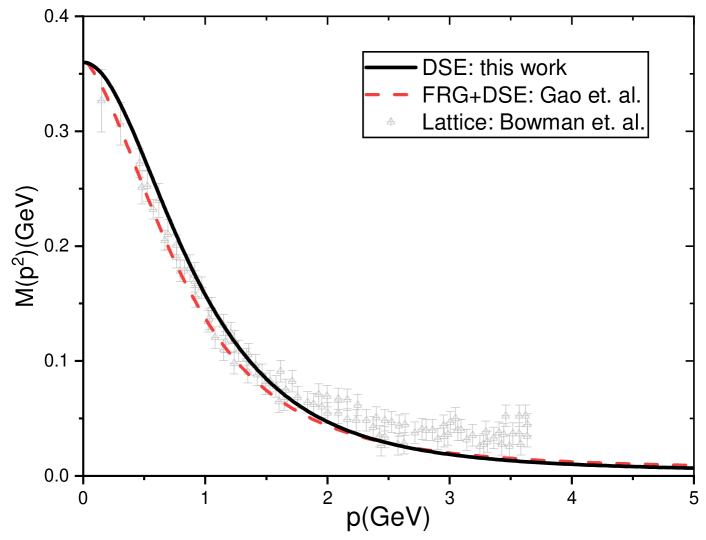
Figure 2: Calculated quark mass function in the vacuum, and the comparison with the lattice QCD result Bowman et al. (2005) and the fully coupled functional QCD result Gao et al. (2021).

which is consistent with the results from the lattice QCD simulation Bowman et al. (2005) and also the fRG-DSE calculation Gao et al. (2021). Moreover, we focus on the quark condensate $\langle\bar{\psi}\psi\rangle$ which can be calculated from the quark propagator:

$$\langle\bar{\psi}\psi\rangle=Z_{2}Z_{m}N_{c}T\sum_{n}\int\frac{d^{3}\vec{\,p}}{(2\pi)^{3}}{\text{tr}}[S(\tilde{\omega}_{n},\vec{\,p})]\,,$$ (12)

For a non-zero bare quark mass $m_{l}$, Eq. (12) will be linearly divergent. Here, one of the regularization scheme is to eliminate the divergent part via the derivative form as done in Refs. Gao and Liu (2016); Gao et al. (2021):

$$\langle\bar{\psi}\psi\rangle_{\mathrm{reg}}=\langle\bar{\psi}\psi\rangle-m\frac{\partial}{\partial m}\langle\bar{\psi}\psi\rangle.$$ (13)

Another choice is the reduced condensate, defined from the strange quark condensate in Refs. Fischer et al. (2014); Lu et al. (2023a)

$$\langle\bar{\psi}\psi\rangle_{\mathrm{red}}=\langle\bar{\psi}\psi\rangle^{l}-\frac{m_{l}}{m_{s}}\langle\bar{\psi}\psi\rangle^{s}\,,$$ (14)

with $m_{s}=27\,m_{l}=56.43\,\textrm{MeV}$. With the same quark propagator as in Eq. (2), we obtained the regularized condensate from Eq. (13) $\langle\bar{\psi}\psi\rangle_{\mathrm{reg}}=(333.6\,\textrm{MeV})^{3}$, and the reduced condensate from Eq. (14) as $(335.8\,\textrm{MeV})^{3}$. Also, the regularized quark condensate satisfies the Gell-Mann-Oakes-Renner Relation:

$$f_{\pi}^{2}m^{2}_{\pi}=2m^{\zeta}\langle\bar{\psi}\psi\rangle_{\zeta}\,,$$ (15)

with the vacuum pion decay constant $f_{\pi}=89\,\textrm{MeV}$ and the pion mass $m_{\pi}=140\,\textrm{MeV}$.

At finite temperature and chemical potential, one can make use of the maximum of the light-quark chiral susceptibility $\chi_{m}^{l}$ to determine the pseudo-critical temperatures, which is defined from the chiral condensate as

$$\chi_{m}^{l}=\frac{\partial\langle\bar{\psi}\psi\rangle_{\mathrm{reg}}}{\partial m_{l}}\,,$$ (16)

For the reduced condensate Eq. (14), the expression of $\chi_{m}$ can be reduced to ${\partial\langle\bar{\psi}\psi\rangle^{l}}/{\partial m_{l}}$ due to the small variations on the strange condensate according to $m_{l}$. Based on this, we take a further approximation of Eq. (16) as:

$$\chi=\frac{\partial B_{0}}{\partial m_{l}}$$ (17)

where $B_{0}$ is the value of $B$ at the first Matsubara frequency and zero three-momentum $B(\tilde{\omega}_{0},\bm{0})$. Such an approximation has been confirmed to be efficient in, e.g., Ref. Gao and Liu (2016), with only a few MeV difference of the extracted pseudo-critical temperatures. Then we obtain the phase transition line as displayed in Fig. 3.

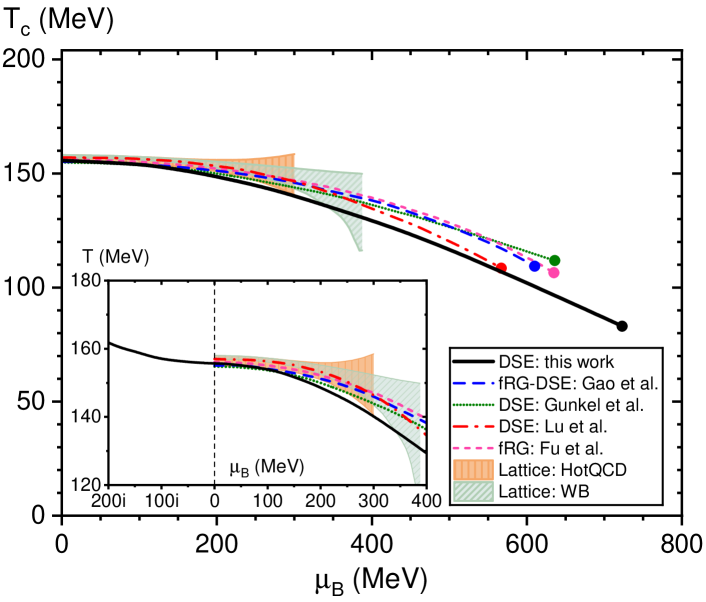
Figure 3: The obtained phase diagram of the chiral phase transition identified with the susceptibility Eq. (16), compared with the lattice QCD Borsanyi et al. (2020); Bazavov et al. (2019) and other functional QCD Gao and Pawlowski (2021); Gunkel and Fischer (2021); Lu et al. (2023a); Fu et al. (2020) results. The solid dots denote the positions of the CEP. A comparison between pure imaginary and real $\mu_{B}$ is also shown in the sub-figure.

At zero chemical potential, our obtained pseudo-critical temperature is $T_{c}=155.7\,\textrm{MeV}$, which is close to the up-to-date lattice QCD results Borsanyi et al. (2020); Bazavov et al. (2019) and the functional QCD results Gao and Pawlowski (2021); Lu et al. (2023a); Gunkel and Fischer (2021); Fischer et al. (2014); Fu et al. (2020). At larger chemical potential and lower temperature, the chiral susceptibility as a function of $T$ and $\mu$ becomes sharper and sharper, and the critical temperature decreases. Such quantitative nature is embedded in the curvature of the phase transition line:

$$\frac{T_{c}(\mu_{B})}{T_{c}(0)}=1-\kappa_{2}^{B}\left(\frac{\mu_{B}}{T_{c}(0)}\right)^{2}+\kappa_{4}^{B}\left(\frac{\mu_{B}}{T_{c}(0)}\right)^{4}+\cdots\,.$$ (18)

The curvature $\kappa_{2}^{B}$ is extracted from a region of $\mu_{B}\in(0,360)\,\textrm{MeV}$ with a result $\kappa_{2}^{B}=0.026$. We also check for the pure imaginary chemical potential in a range of $\mu_{B}^{2}\in(-210^{2},0)\,\textrm{MeV}^{2}$, and obtain the corresponding curvature $\kappa_{2}^{B}=0.024$. The phase transition line at real and pure imaginary $\mu_{B}$ is displayed together in Fig. 3, which shows that the continuity is valid at zero $\mu_{B}$, in agreement with what is found in Ref. Bernhardt and Fischer (2023). Eventually, the susceptibility is divergent at the location of CEP, which is found at $(T_{CEP},\mu_{B,CEP})=(83\,\textrm{MeV},723\,\textrm{MeV})$. Compared with a similar truncation scheme as in Ref. Fischer et al. (2014), one can notice that the $T_{CEP}$ is almost the same, but the $\mu_{B,CEP}$ is larger due to a different treatment on the gluon sector.

III The Lee Yang edge singularities

In Refs. Yang and Lee (1952); Lee and Yang (1952), Lee and Yang have revealed the relation between phase transition and the zeroes of partition functions $Z$ on the $\mu$ complex plane: the Lee-Yang Zeroes. These zeroes form branch cuts on the $\mu$ plane, and the edge branch points are known as Lee Yang edge (LYE) singularities. In short, when the LYE singularities reach the $\mu$ real axis, the singularities correspond to the critical end point. While the branch cut crosses the real axis, the first order phase transition occurs. These can be well understood due to the properties of pressure $P=\frac{1}{V}T\ln Z$ around the Lee-Yang Zeroes. Briefly speaking, the first derivative of $P$ is discontinuous crossing the branch cut, and continuous but non-analytical at the LYE singularities. This suggests that the same criterion, i.e. the susceptibility $\chi$ in Eq. (16) for the phase transition line introduced in Sec. II can also be applied to determine the location of LYE singularities, when the chemical potential is extended to the complex values.

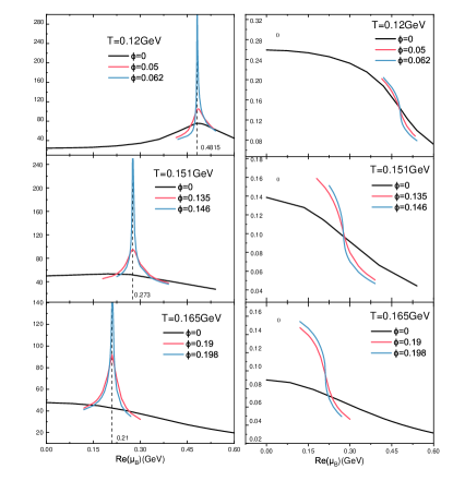
Figure 4: The obtained complex chemical potential dependence of chiral susceptibility $\chi$ in Eq. (17) (left panels) and the mass $M_{0}$ (right panels) at temperatures $T=120\,\textrm{MeV}$ (the first row), $T=151\,\textrm{MeV}$ (the second row), $T=165\,\textrm{MeV}$ (the third row). The singularities are marked by the dashed lines which correspond to the critical chemical potentials.

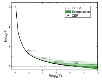
Figure 5: The obtained trajectory of the LYE singularities on the ${\text{Re}}(\mu_{B}/T)$ – ${\text{Im}}(\mu_{B}/T)$ plane, together with the CEP which is marked on the ${\text{Im}}(\mu_{B}/T)=0$ axis. The extrapolation analysis of the trajectory using data within ${\text{Re}}(\mu_{B}/T)\in(0,2)$, $(0,4)$ and $(0,6)$ are also shown with the error estimates, which are displayed as the light, medium and dark colored bands, respectively.

In specific, we scan the $\chi$ over the $T-{\text{Re}}\,\mu$ plane at a given imaginary chemical potential ${\text{Im}}\,\mu=\phi\pi T$ for $\phi\in(0,1)$, and the obtained result is illustrated in Fig. 4. It can be seen that when $T>T_{CEP}$, there exist apparent singularities on the complex $\mu$ plane. For example, at $T=120\,\textrm{MeV}$, the susceptibility $\chi$ is continuous along ${\text{Re}}(\mu)$ at $\phi=0$. As $\phi$ approaches the critical value $\phi_{c}=0.062$, $M_{0}$ becomes steeper with a sharper peak of $\chi$ and finally reaches the singularity at ${\text{Re}}\,{\mu_{LYE}}=481.5\,\textrm{MeV}$. For a higher temperature, e.g. $T=150\,\textrm{MeV}$, one can observe a similar behavior of $\chi$. Also, at $T>T_{c}$ the singularity still exists in the complex $\mu_{B}$ plane. The edge of such singularity $\mu_{LYE}$ is scanned in a wide range of temperature to yield a trajectory of the LYE singularities, the obtained results are displayed in Fig. 5. Our result shows apparently that the trajectory crosses the real axis of $\mu_{B}$ exactly at $T=T_{CEP}$, which implies a strong connection between the QCD critical end point and the LYE singularities.

We then provide an estimate on the critical region of CEP via an extrapolation study of the obtained $\mu_{LYE}$ data. In specific, we consider the data within several small chemical potential regions and carry out the extrapolation with the convergent Padé polynomials (in $N=n\,m,\,n\in[1,2],\ m\in[n,3]$) towards a higher ${\text{Re}}\,\mu_{B}$ to compare with the calculated trajectory and also the CEP position. The regions we take are ${\text{Re}}(\mu_{B}/T)\in[0,2]$, $[0,4]$ and $[0,6]$ and the corresponding analyses are shown in Fig. 5. It is found that the quality of the extrapolation becomes better with an extending range of ${\text{Re}}(\mu_{B}/T)$ being included. Within ${\text{Re}}(\mu_{B}/T)\in[0,2]$ where the lattice extrapolation approach is still controllable, the extrapolated position of the CEP has a systematic error of more than $30\%$. It is also estimated that a knowledge of ${\text{Re}}(\mu_{B}/T)$ with the range corresponds to $\Delta T=|T/T_{CEP}-1|\sim 20\%$ and $\Delta\mu=|\mu/\mu_{B,CEP}-1|\sim 15\%$, is required in order to get an error control of 10% for the extrapolated CEP. In short, additional information at large ${\text{Re}}\,\mu_{B}$ is still required in order to provide a precise determination of the CEP position.

IV Analysing the trajectory of the LYE singularities

In the vicinity of the LYE singularities where the second-order phase transition occurs, the correlation length tends to be divergent, and the critical behavior is only determined by the symmetry and dimension of the system which can be classified into various universality classes. Then one can describe the critical behavior including the location of LYE singularities of a specific system by universal quantities and the non-universal relevant thermodynamic parameters. For the Ising model and $O(N)$ model, expressed by the scaling field $z$, the singularities locate at $z=t/h^{1/\beta\delta}=|z_{c}|e^{i\pi/2\beta\delta}$ Basar (2021); Zinn-Justin (2021), where $t$ and $h$ the general scaling variables with $t$ being the reduced temperature, and $h$ being the symmetry breaking field. $|z_{c}|,\beta,\delta$ are universal scaling parameters which can be determined in the universality class analysis, and some of which are listed in Table 1.

In the chiral limit, the QCD Lagrangian has $SU_{R}(2)\times SU_{L}(2)\cong O(4)$ symmetry. Therefore, for a small quark mass, the critical behavior is expected to be described by the 3D $O(4)$ universality class. According to Refs. Kaczmarek et al. (2011); Mukherjee and Skokov (2021), the thermodynamic parameters $T$, $\mu_{B}$ and with the light-to-strange quark mass ratio $m_{l}/m_{s}$ can be mapped onto the scaling variables $t$ and $h$ at zero chemical potential as:

$$t= \,t_{0}^{-1}\left[\frac{T-T_{c}^{0}}{T_{c}^{0}}+\kappa_{2}^{B}\left(\frac{\mu_{B}}{T_{c}^{0}}\right)^{2}\right]\,,$$ (19)

$$h= \,h_{0}^{-1}\frac{m_{l}}{m_{s}}\,,$$

from which one can derive the expression for the location of the singularities at specific temperature Mukherjee and Skokov (2021):

$$\left(\mu_{LYE}\right)^{2}=\frac{(T_{c}^{0})^{2}}{\kappa_{2}^{B}}\left[\frac{|z_{c}|}{z_{0}}e^{i\pi/2\beta\delta}\left(\frac{m_{l}}{m_{s}}\right)^{\frac{1}{\beta\delta}}-\frac{T-T^{0}_{c}}{T^{0}_{c}}\right]\,,$$ (20)

where $\kappa_{2}^{B}$ is the curvature of the phase transition line and $T_{c}^{0}$ the phase transition temperature at zero chemical potential in chiral limit. In turn, the singularity also corresponds to the convergence radius of the expansion with respect to the chemical potential. As determined in the last section, we have $\kappa_{2}^{B}=0.026$ and $m_{l}/m_{s}=1/27$. The remaining parameters are $T_{c}^{0}$ and $z_{0}$, the former of which can be interpreted as the critical temperature in the chiral limit. With our truncation scheme Eq. (6), such critical temperature is found at $T_{c}^{0}=0.138\,\text{GeV}$. Also, the scale factor expected to be $z_{0}\in(1,2)$ Mukherjee and Skokov (2021) and here we simply take $z_{0}=1.5$.

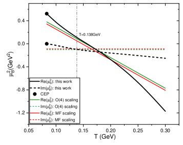
Figure 6: The obtained temperature dependence of the squared complex chemical potential of the LYE singularity $\mu_{LYE}^{2}$, including its real part (solid line) and imaginary part (dashed line), respectively. The dashed vertical line is at $T_{c}^{0}=138$ MeV. The case of CEP is also marked with the black solid dots.

Table 1: The critical exponents $\beta$, $\delta$ and the location of Lee Yang Edge Singularities $|z_{c}|$ for different universality classes  Connelly et al. (2020); Johnson et al. (2023); Rennecke and Skokov (2022); Kos et al. (2016).

	$\beta$	$\delta$	$|z_{c}|$
$3d\,\,Z(2)$	0.33	4.79	2.43
$3d\,\,O(4)$	$0.38$	$4.82$	$1.69$
Mean field	0.5	3	1.89

On the other hand, the quark gap equation under the current truncation scheme is expected to be in the mean field universality class. To investigate this, we take Eq. (20) to explore the scaling behavior of the singularities. In specific, we study the temperature dependence of $\mu_{LYE}^{2}$ for both its real and the imaginary part, which is shown explicitly in Figure 6. For the real part of $\mu_{LYE}^{2}$, the $T$ dependence is approximately linear, as expected in Eq. (20). However, the $T$ dependence of ${\text{Im}}\mu_{LYE}^{2}$ is not negligible, not only close to the CEP but also at $T=T_{c}^{0}=0.138\,\textrm{GeV}$. This suggests an additional temperature dependence of the $z_{c}$ and thus a deviation of the scaling behavior to either the 3D $O(N)$ or the mean field universality class, for a physical quark mass.

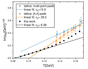
Figure 7: The scaling behavior of the imaginary part of the chemical potential and a linear fit of $\mathrm{Im}[\mu_{B}]^{1/(\beta\delta)}$ and $T$ together with the LYE singularities from lattice simulations Goswami et al. (2024); Dimopoulos et al. (2022); Bollweg et al. (2022). The parameter $c_{2}$ can be directly extracted from the slope, and applied to estimate the CEP location. Generally speaking, for larger $c_{2}$ , one typically gets a larger temperature for CEP.

Finally, consider the region near the CEP, the universality class is expected to be Z(2) symmetry. By performing the linear mapping of the thermodynamic parameters $(T,\mu_{B})$ to the scaling variables $(t,h)$:

$$\left(\begin{array}[]{c}t\\[2.84526pt] h\end{array}\right)=\mathbb{M}\left(\begin{array}[]{c}T-T_{CEP}\\[2.84526pt] \mu_{B}-\mu_{B,CEP}\end{array}\right),\,\quad\mathbb{M}=\left(\begin{array}[]{ll}t_{T}&t_{\mu}\\[2.84526pt] h_{T}&h_{\mu}\end{array}\right)\,,\quad$$ (21)

one can derive the Z(2) scaling formula of the LYE singularitiesBasar (2021); Stephanov (2006):

$$\mu_{LYE} \sim\mu_{B,CEP}-c_{1}(T-T_{CEP})+\textrm{i}c_{2}(T-T_{CEP})^{\beta\delta},$$ (22)

with $$c_{1}=\frac{h_{T}}{h_{\mu}},\quad c_{2}=x_{LY}\frac{t_{\mu}{}^{\beta\delta}}{h_{\mu}}\left(\frac{t_{T}}{t_{\mu}}-\frac{h_{T}}{h_{\mu}}\right)^{\beta\delta}.$$

where $x_{LY}$ the imaginary part of LYE singularity in Ising model and $x_{LY}=|z_{c}|^{-\beta\delta}$.

By analysing the scaling behavior of the imaginary part of chemical potential with respect to the reduced temperature as shown in Fig. 7, the critical region can be determined as $\ln((T-T_{CEP})/T_{CEP})<-1$, i.e. $T\in[83,110]\,\text{MeV}$. The extracted critical exponents is $\beta\delta=1.38$, which slightly differs from the exact value of $Z(2)$ universality class shown in Table 1 due to the lack of detailed critical information in current truncation scheme. However, the CEP scaling behavior is clear and the constants $c_{1}$ and $c_{2}$ in Eq. (22) can be estimated by fitting with our results within the critical region. The corresponding CEP scaling trajectory is obtained and extrapolated towards small ${\text{Re}}\,\mu_{B}$, shown as the green line in Fig. 8, which shows that the CEP scaling extrapolation is consistent with the calculated trajectory near CEP.

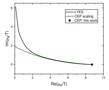
Figure 8: The LYE singularities trajectory (black), which is well compared with the extracted CEP scaling trajectory (green) from Eq. (22).

Our results show that the Z(2) scaling works for the LYE singularities, and therefore, one may directly apply the Ising parameterization to study CEP. Firstly, we apply the following parameterization as it can well describe the equation of state of QCD Lu et al. (2023b); Parotto et al. (2020); Rehr and Mermin (1973). Typically, we take the form as shown in Ref. Lu et al. (2023b):

$$\frac{\,\mu_{B}-\mu_{B,CEP}\,}{\mu_{B,CEP}}=-t\omega\rho\cos{\alpha_{1}}-h\omega\cos{\alpha_{2}},$$ (23)

$$\frac{T-T_{CEP}}{T_{CEP}}=f_{\mathrm{PT}}(t)+h\omega\sin{\alpha_{2}},$$

with $\omega=1$, $\rho=2$, $\alpha_{1}=\tan^{-1}(2\kappa\mu_{B,CEP}/T_{c}(0))$ and $\alpha_{2}=\alpha_{1}+\pi/2$ in our case. The mapping function $f_{\mathrm{PT}}$ is calibrated so that at $h=0$, Eqs. (23) becomes exactly the parametric equations of the phase transition line in Eq. (18), which requires

$$f_{\mathrm{PT}}(t)=\frac{\,\mu_{B,CEP}\,}{2T_{CEP}}\left(2-t\omega\rho\cos{\alpha_{1}}\right)\,t\omega\rho\sin{\alpha_{1}}.$$ (24)

This then gives immediately the parameter $c_{2}$ as:

$$\bar{c}_{2} =x_{LY}\frac{(\frac{T_{CEP}}{\,\mu_{B,CEP}\,})^{\beta\delta}\omega\sin{\alpha_{1}}}{(\omega\rho\sin{\alpha_{1}})^{\beta\delta}}\left(\frac{T_{CEP}}{\mu_{B,CEP}}\cot^{2}{\alpha_{1}}+1\right),$$ (25)

with $\bar{c}_{2}=c_{2}\frac{(T_{CEP})^{\beta\delta}}{\mu_{B,CEP}}$ the dimensionless parameter to avoid the error from the scale setting in the truncation scheme. Together with the parameterization of phase transition line for CEP as:

$$T_{CEP}=T_{c}(0)-\kappa\frac{\mu_{B,CEP}^{\,2}}{T_{c}(0)},$$ (26)

the location of CEP can be determined after one extracts $c_{2}$ from the numerical results of LYE singularities in QCD. In Fig. 7, we show the extraction of $c_{2}$ from the LYE singularities.

Through the linear fit between ${\text{Im}}[\mu_{B}]^{1/(\beta\delta)}$ and $T$, one can extract $c_{2}$ directly from the slope, and we get $c_{2}=6.38\,\textrm{GeV}^{1-\beta\delta}$ and $\bar{c}_{2}=0.28$. Now if here we adopt $\beta\delta$ and $z_{c}$ from $Z(2)$ universality class and the phase transition line curvature $\kappa=0.016$ and $T_{c}(0)=156\,\textrm{MeV}$, one gets the CEP at:

$$(T_{CEP},\mu_{B,CEP})=(118,606)\,\,\mathrm{MeV},$$ (27)

which means that with the $\bar{c}_{2}$ extracted in our work together with the up to date knowledge of the phase transition line and the correct scaling behavior, the obtained CEP location is in precisely good agreement with the up to date results from the functional QCD approaches Fu et al. (2020); Gao and Pawlowski (2020, 2021); Gunkel and Fischer (2021). Besides, the rescaled $c^{\prime}_{2}$ based on the estimated CEP now becomes $c^{\prime}_{2}=5.0\,\textrm{GeV}^{1-\beta\delta}$. It needs also to mention that one may get a much larger $c_{2}$ from the current results of LYE singularities from lattice simulations Goswami et al. (2024); Dimopoulos et al. (2022); Bollweg et al. (2022). It is mainly because the current lattice QCD results are obtained in too high temperature region and has not reached the scaling region as shown in Fig. 7. For the LYE singularities next to the CEP scaling region, the slope is steeper which then stands for a large value of $c_{2}$.

V Summary

We calculate the quark gap equation at complex chemical potential with physical quark mass. We firstly check the analytic continuity of the phase transition line from imaginary to real chemical potential, which is required in the lattice QCD simulation. Our result shows that the curvature of the chiral phase transition extracted from the imaginary chemical potential is consistent with the one from the real chemical potential.

Moreover, we study the Lee-Yang edge singularities which has been shown to be related to the phase structure of the phase transition at real chemical potential. We compute the location of the Lee-Yang edge singularities in the complex $\mu_{B}$ plane for different temperatures. Our result manifests that, at the temperature where there is crossover at the real chemical potential, the Lee-Yang edge singularity is located at complex plane of chemical potential with an imaginary part. The absolute value of the imaginary part becomes smaller as the temperature decreases, and finally vanishes at the critical end point temperature.

We then take the Padé polynomials to see whether it is possible to extrapolate the CEP location with the limited range of the Lee-Yang edge singularities. Our result indicates that additional information at high $\mu_{B}$, especially beyond the range of current best lattice QCD expansions, is required from the theoretical approaches for a precise determination of the CEP.

We further check the scaling behavior of the trajectory of Lee-Yang edge singularities. We compute the radius of the convergence and find that it changes for different temperatures. The value of the convergence radius is also found to be inconsistent with any scaling value for either 3D $O(N)$ or mean field universality class. However, it is found that the LYE singularities follows the CEP scaling as the $Z(2)$ universality class. Therefore, one may take the Ising model to study the CEP of QCD. Here we implement a mapping of the QCD order parameters with Ising parameterization, and shows that after extracting $c_{2}$ from the current data of the LYE singularities location together with the curvature of the phase transition line, one may extract the location of CEP with the information of Ising universality class.

For a high temperature, the real part of the Lee-Yang edge singularities becomes smaller and the imaginary part increases which is consistent with the perturbative analysis. The imaginary part is expected to be saturated at ${\text{Im}}\,\mu_{B}=3\pi T$ which requires a careful scan for a wide range of the complex chemical potential. This may also reveal the periodicity of the thermodynamic quantities which represents the $Z(N_{c})$ symmetry and potentially the deconfinement. The related investigation is under progress.

VI Acknowledgements

YL and FG thank the other members of the fQCD collaboration Braun et al. (2023) for fruitful discussions. This work is supported by the National Natural Science Foundation of China under Grants No. 12247107, No. 12175007. FG is also supported by the National Science Foundation of China under Grants No. 12305134.

References

- Aarts et al. (2023) G. Aarts et al., Prog. Part. Nucl. Phys. 133, 104070 (2023), arXiv:2301.04382 [hep-lat] .
- Hippert et al. (2023) M. Hippert, J. Grefa, T. A. Manning, J. Noronha, J. Noronha-Hostler, I. Portillo Vazquez, C. Ratti, R. Rougemont, and M. Trujillo, (2023), arXiv:2309.00579 [nucl-th] .
- Huang and Zhuang (2023) M. Huang and P. Zhuang, Symmetry 15, 541 (2023).
- Fu (2022) W. J. Fu, Commun. Theor. Phys. 74, 097304 (2022), arXiv:2205.00468 [hep-ph] .
- Lovato et al. (2022) A. Lovato et al., (2022), arXiv:2211.02224 [nucl-th] .
- Adamczewski-Musch et al. (2019) J. Adamczewski-Musch et al. (HADES), Nature Phys. 15, 1040 (2019).
- Fischer (2019) C. S. Fischer, Prog. Part. Nucl. Phys. 105, 1 (2019), arXiv:1810.12938 [hep-ph] .
- Luo and Xu (2017) X. Luo and N. Xu, Nucl. Sci. Tech. 28, 112 (2017), arXiv:1701.02105 [nucl-ex] .
- Braun-Munzinger et al. (2016) P. Braun-Munzinger, V. Koch, T. Schäfer, and J. Stachel, Phys. Rept. 621, 76 (2016), arXiv:1510.00442 [nucl-th] .
- Schaefer and Wagner (2009) B.-J. Schaefer and M. Wagner, Prog. Part. Nucl. Phys. 62, 381 (2009), arXiv:0812.2855 [hep-ph] .
- Gao and Pawlowski (2021) F. Gao and J. M. Pawlowski, Phys. Lett. B 820, 136584 (2021), arXiv:2010.13705 [hep-ph] .
- Gunkel and Fischer (2021) P. J. Gunkel and C. S. Fischer, Phys. Rev. D 104, 054022 (2021), arXiv:2106.08356 [hep-ph] .
- Gao and Pawlowski (2020) F. Gao and J. M. Pawlowski, Phys. Rev. D 102, 034027 (2020), arXiv:2002.07500 [hep-ph] .
- Fu et al. (2020) W. J. Fu, J. M. Pawlowski, and F. Rennecke, Phys. Rev. D 101, 054032 (2020), arXiv:1909.02991 [hep-ph] .
- Cai et al. (2022) R.-G. Cai, S. He, L. Li, and Y.-X. Wang, Phys. Rev. D 106, L121902 (2022), arXiv:2201.02004 [hep-th] .
- Yang and Lee (1952) C.-N. Yang and T. D. Lee, Phys. Rev. 87, 404 (1952).
- Lee and Yang (1952) T. D. Lee and C.-N. Yang, Phys. Rev. 87, 410 (1952).
- Clarke et al. (2023) D. A. Clarke, K. Zambello, P. Dimopoulos, F. Di Renzo, J. Goswami, G. Nicotra, C. Schmidt, and S. Singh, PoS LATTICE2022, 164 (2023), arXiv:2301.03952 [hep-lat] .
- Schmidt et al. (2023) C. Schmidt, D. A. Clarke, G. Nicotra, F. Di Renzo, P. Dimopoulos, S. Singh, J. Goswami, and K. Zambello, Acta Phys. Polon. Supp. 16, 1 (2023), arXiv:2209.04345 [hep-lat] .
- Singh et al. (2022) S. Singh, P. Dimopoulos, L. Dini, F. Di Renzo, J. Goswami, G. Nicotra, C. Schmidt, K. Zambello, and F. Ziesche (Bielefeld-Parma), PoS LATTICE2021, 544 (2022), arXiv:2111.06241 [hep-lat] .
- Roberge and Weiss (1986) A. Roberge and N. Weiss, Nucl. Phys. B 275, 734 (1986).
- Fischer et al. (2015) C. S. Fischer, J. Luecker, and J. M. Pawlowski, Phys. Rev. D 91, 014024 (2015), arXiv:1409.8462 [hep-ph] .
- Fischer (2009) C. S. Fischer, Phys. Rev. Lett. 103, 052003 (2009), arXiv:0904.2700 [hep-ph] .
- Fischer et al. (2011) C. S. Fischer, J. Luecker, and J. A. Mueller, Phys. Lett. B 702, 438 (2011), arXiv:1104.1564 [hep-ph] .
- Alkofer and von Smekal (2001) R. Alkofer and L. von Smekal, Phys. Rept. 353, 281 (2001), arXiv:hep-ph/0007355 .
- Roberts (2008) C. D. Roberts, Prog. Part. Nucl. Phys. 61, 50 (2008), arXiv:0712.0633 [nucl-th] .
- Fischer et al. (2014) C. S. Fischer, J. Luecker, and C. A. Welzbacher, Phys. Rev. D 90, 034022 (2014), arXiv:1405.4762 [hep-ph] .
- Gao et al. (2021) F. Gao, J. Papavassiliou, and J. M. Pawlowski, Phys. Rev. D 103, 094013 (2021), arXiv:2102.13053 [hep-ph] .
- Bowman et al. (2005) P. O. Bowman, U. M. Heller, D. B. Leinweber, M. B. Parappilly, A. G. Williams, and J.-b. Zhang, Phys. Rev. D 71, 054507 (2005), arXiv:hep-lat/0501019 .
- Gao and Liu (2016) F. Gao and Y. X. Liu, Phys. Rev. D 94, 076009 (2016), arXiv:1607.01675 [hep-ph] .
- Lu et al. (2023a) Y. Lu, F. Gao, Y. X. Liu, and J. M. Pawlowski, (2023a), arXiv:2310.18383 [hep-ph] .
- Borsanyi et al. (2020) S. Borsanyi, Z. Fodor, J. N. Guenther, R. Kara, S. D. Katz, P. Parotto, A. Pasztor, C. Ratti, and K. K. Szabo, Phys. Rev. Lett. 125, 052001 (2020), arXiv:2002.02821 [hep-lat] .
- Bazavov et al. (2019) A. Bazavov et al. (HotQCD), Phys. Lett. B 795, 15 (2019), arXiv:1812.08235 [hep-lat] .
- Bernhardt and Fischer (2023) J. Bernhardt and C. S. Fischer, Eur. Phys. J. A 59, 181 (2023), arXiv:2305.01434 [hep-ph] .
- Basar (2021) G. Basar, Phys. Rev. Lett. 127, 171603 (2021), arXiv:2105.08080 [hep-th] .
- Zinn-Justin (2021) J. Zinn-Justin, Quantum field theory and critical phenomena, International Series of Monographs on Physics, Vol. 77 (Oxford University Press, 2021).
- Kaczmarek et al. (2011) O. Kaczmarek, F. Karsch, E. Laermann, C. Miao, S. Mukherjee, P. Petreczky, C. Schmidt, W. Soeldner, and W. Unger, Phys. Rev. D 83, 014504 (2011), arXiv:1011.3130 [hep-lat] .
- Mukherjee and Skokov (2021) S. Mukherjee and V. Skokov, Phys. Rev. D 103, L071501 (2021), arXiv:1909.04639 [hep-ph] .
- Connelly et al. (2020) A. Connelly, G. Johnson, F. Rennecke, and V. Skokov, Phys. Rev. Lett. 125, 191602 (2020), arXiv:2006.12541 [cond-mat.stat-mech] .
- Johnson et al. (2023) G. Johnson, F. Rennecke, and V. V. Skokov, Phys. Rev. D 107, 116013 (2023), arXiv:2211.00710 [hep-ph] .
- Rennecke and Skokov (2022) F. Rennecke and V. V. Skokov, Annals Phys. 444, 169010 (2022), arXiv:2203.16651 [hep-ph] .
- Kos et al. (2016) F. Kos, D. Poland, D. Simmons-Duffin, and A. Vichi, JHEP 08, 036 (2016), arXiv:1603.04436 [hep-th] .
- Goswami et al. (2024) J. Goswami, D. A. Clarke, P. Dimopoulos, F. Di Renzo, C. Schmidt, S. Singh, and K. Zambello, (2024), arXiv:2401.05651 [hep-lat] .
- Dimopoulos et al. (2022) P. Dimopoulos, L. Dini, F. Di Renzo, J. Goswami, G. Nicotra, C. Schmidt, S. Singh, K. Zambello, and F. Ziesché, Phys. Rev. D 105, 034513 (2022).
- Bollweg et al. (2022) D. Bollweg, J. Goswami, O. Kaczmarek, F. Karsch, S. Mukherjee, P. Petreczky, C. Schmidt, and P. Scior (HotQCD), Phys. Rev. D 105, 074511 (2022), arXiv:2202.09184 [hep-lat] .
- Stephanov (2006) M. A. Stephanov, Phys. Rev. D 73, 094508 (2006).
- Lu et al. (2023b) Y. Lu, F. Gao, B.-C. Fu, H.-C. Song, and Y. X. Liu, (2023b), arXiv:2310.16345 [hep-ph] .
- Parotto et al. (2020) P. Parotto, M. Bluhm, D. Mroczek, M. Nahrgang, J. Noronha-Hostler, K. Rajagopal, C. Ratti, T. Schäfer, and M. Stephanov, Phys. Rev. C 101, 034901 (2020).
- Rehr and Mermin (1973) J. J. Rehr and N. D. Mermin, Phys. Rev. A 8, 472 (1973).
- Braun et al. (2023) J. Braun, Y. R. Chen, W. J. Fu, F. Gao, A. Geissel, J. Horak, C. Huang, F. Ihssen, Y. Lu, J. M. Pawlowski, F. Rennecke, F. Sattler, B. Schallmo, J. Stoll, Y. Y. Tan, S. Töpfel, J. Turnwald, R. Wen, J. Wessely, N. Wink, S. Yin, and N. Zorbach, (2023).