Dissipative particle dynamics for coarse-grained models

Abstract

We develop a computational method based on Dissipative Particle Dynamics (DPD) that introduces solvent hydrodynamic interactions to coarse-grained models of solutes, such as ions, molecules, or polymers. DPD-solvent (DPDS) is a fully off-lattice method that allows straightforward incorporation of hydrodynamics at desired solvent viscosity, compressibility and solute diffusivity with any particle-based solute model. Solutes interact with the solvent only through the DPD thermostat, which ensures that the equilibrium properties of the solute system are not affected by the introduction of the DPD solvent. Thus, DPDS can be used as a replacement for traditional molecular dynamics thermostats such as Nosé-Hoover and Langevin. We demonstrate the applicability of DPDS on the case of polymer dynamics and electroosmotic flow through a nanopore. The method should be broadly useful as means to introduce hydrodynamics to existing coarse-grained models of molecules and soft materials.

Coarse-grained implicit-solvent models are usually parametrized to produce a desired equilibrium distribution of states. To use the same models in non-equilibrium simulations with desired transport properties and hydrodynamic behavior requires a method that introduces hydrodynamic interactions at the specific solvent viscosity, compressibility and solute diffusivity without affecting the equilibrium configurational properties of the system.

To achieve this, the coarse-grained system can be coupled to a mesh, typically a cubic grid, and hydrodynamics is solved using this mesh. A few examples of such approaches include Multi-Particle Collision dynamics (MPC) or Stochastic Rotation Dynamics Malevanets and Kapral (1999); Gompper et al. (2009), Lattice Boltzmann (LB) methods Krueger et al. (2016), and Fluid Particle Dynamics (FPD) Tanaka and Araki (2000). However, coupling of the continuous system to a mesh can introduce artifacts and increase propagation errors. MPC does not conserve angular momentum (or breaks time-reversal symmetry) and suffers from artificially high compressibility Gompper et al. (2009). LB allows embedding of large colloids, but embedding of particles smaller than the lattice size, e.g., polymers, suffers from lattice discretization errors and mixing molecular dynamics with LB propagation leads to energy conservation issues Dünweg and Ladd (2009). FPD directly solves the Navier–Stokes equations but can only embed objects at least a few lattice sites in size, which makes the method suitable for nanoparticles and colloids Furukawa et al. (2018), but is computationally inefficient for small molecules, ions or polymers.

Among off-lattice approaches the most straightforward way to partially introduce hydrodynamics is to apply a Galilean-invariant thermostat directly to the solute particles Soddemann et al. (2003), however, this approach requires a dense suspension and is not applicable to dilute solutions. A general off-lattice method is Dissipative Particle Dynamics (DPD) that simulates hydrodynamic interactions by representing the fluid as soft particles Hoogerbrugge and Koelman (1992); Groot and Warren (1997). DPD reproduces a desired solvent viscosity and compressibility while describing thermal fluctuations and allowing the explicit representation of different chemical components Espa ol and Warren (2017). However, simply adding DPD particles to a coarse-grained system introduces depletion effects and thus changes the equilibrium properties of the system. While it is possible to model a variety of multicomponent systems by modifying the conservative interactions between DPD particles Pagonabarraga and Frenkel (2001); Groot and Rabone (2001), this approach requires careful parametrization; altering conservative interactions does not merely change the equilibrium properties but also transport behavior such as local viscosity, compressibility and diffusivity. Furthermore, point charges cannot be included due to the DPD soft repulsive potentials Groot (2003).

Here we propose an alternative off-lattice method, named DPD solvent (DPDS), that incorporates hydrodynamic interactions in coarse-grained models of solutes. The premise of the method is overlay the DPD fluid at desired viscosity and compressibility with the solute system. The DPD solvent interacts with the solute system only via the DPD thermostat. Thus, the equilibrium properties of the system and the DPD-solvent are fully decoupled and can be controlled separately, while the transport properties are determined by the solute–solvent thermostat coupling strength. The main advantage of this procedure over existing methods is that it avoids any lattice mapping issues. The same or a similar velocity-Verlet integrator is used to evolve configurations both for the solute system and the DPD solvent, which minimizes propagation errors due to solvent–solute coupling and significantly simplifies the implementation compared to hybrid lattice approaches.

In the following, we review the DPD technique and then show how to combine it with coarse-grained systems of solutes using the DPDS approach. We demonstrate the applicability of DPDS on two typical coarse-grained models, a bead-spring polymer and a primitive model electrolyte, and show that it accurately describes hydrodynamic interactions by investigating polymer collapse, Zimm dynamics and electrokinetic flow in patterned nanochannels.

I review of the DPD fluid properties

The DPD fluid is modeled as a canonical ensemble of soft spherical particles at density $\rho$ and temperature $T$. The particles interact via three distinct interactions. The conservative pair interaction is typically chosen as parabolic repulsion, with the potential energy of an ensemble of $N$ particles

$$V(\mathbf{r}^{N})=\frac{1}{2}\sum_{ij}\begin{cases}a_{ij}(1-r_{ij}/r_{\textnormal{c}})^{2}\;,&\textnormal{for }r_{ij}<r_{\textnormal{c}}\\ 0\;,&\text{otherwise}\;.\end{cases}$$ (1)

The sum proceeds over all particle pairs $i,j$ with $\mathbf{r}_{i}$ the position of particle $i$, $r_{ij}=|\mathbf{r}_{i}-\mathbf{r}_{j}|$ the inter-particle distance and $r_{\textnormal{c}}$ the cutoff length. The prefactor $a_{ij}$ is set to reproduce the desired compressibility of the fluid Groot and Warren (1997) and can be different among different particle types to model multicomponent fluids.

The dissipative friction force between particles $i$ and $j$ is

$$F^{\textnormal{d}}_{ij} = \gamma\omega(r_{ij})^{2}(\mathbf{v}_{ij}\cdot\hat{\mathbf{r}}_{ij})\hat{\mathbf{r}}_{ij}$$ (2)

$$- \gamma_{\perp}\omega_{\perp}(r_{ij})^{2}(\mathbf{I}-\hat{\mathbf{r}}_{ij}\hat{\mathbf{r}}_{ij}^{T})\mathbf{v}_{ij}\;.$$

where the first term describes the friction force parallel to the inter-particle vector $\mathbf{r}_{ij}=\mathbf{r}_{j}-\mathbf{r}_{i}$ with $\hat{\mathbf{r}}_{ij}=\mathbf{r}_{ij}/|\mathbf{r}_{ij}|$ the corresponding unit vector. The friction is proportional to the coefficient $\gamma$ and distance-dependent weighting function $w(r_{ij})$. The second term describes the corresponding perpendicular contribution Junghans et al. (2008), i.e., the shear friction, with coefficient $\gamma_{\perp}$ and weighting function $w_{\perp}(r_{ij})$. $\mathbf{I}$ is the identity matrix and $\hat{\mathbf{r}}_{ij}^{T}$ denotes the transpose of $\hat{\mathbf{r}}_{ij}$.

The fluctuation–dissipation relation implies that the random force between the two particles is given by

$$F^{\textnormal{r}}_{ij} = \sqrt{2\gamma k_{\textnormal{B}}T}\omega(r_{ij})\frac{dW_{ij}}{dt}\hat{\mathbf{r}}_{ij}$$ (3)

$$+ \sqrt{2\gamma_{\perp}k_{\textnormal{B}}T}\omega_{\perp}(r_{ij})\frac{d\mathbf{W}_{ij}}{dt}(\mathbf{I}-\hat{\mathbf{r}}_{ij}\hat{\mathbf{r}}_{ij}^{T})\;,$$

where the prefactors are determined by the desired temperature $T$ of the system, $dW_{ij}$ is the independent increment of a Wiener process and $d{\mathbf{W}}_{ij}$ the vector of independent Wiener processes. For a finite time-step, $\frac{\Delta W_{ij}}{\Delta t}=\zeta_{ij}\Delta t^{-1/2}$, and $\frac{\Delta{\mathbf{W}}_{ij}}{\Delta t}=\bm{\zeta}_{ij}\Delta t^{-1/2}$ where $\zeta_{ij}$ is a symmetric random variable with zero mean and unit variance and $\bm{\zeta}_{ij}$ is the corresponding random vector.

The stochastic differential equations that determine the evolution of the fluid are thus

$$m_{i}\frac{d\mathbf{v}_{i}}{dt} = -\frac{\partial V}{\partial\mathbf{r}_{i}}+\sum_{j}F^{\textnormal{d}}_{ij}+F^{\textnormal{r}}_{ij}\;,$$

$$\frac{d\mathbf{r}_{i}}{dt} = \mathbf{v}_{i}\;.$$ (4)

with $m$ the mass of the DPD particles. These equations are usually evolved using the velocity-Verlet integrator Groot and Warren (1997); Pagonabarraga et al. (1998) and the DPD model is implemented in various open-source molecular dynamics (MD) packages such as LAMMPS, EPResSo and HOOMD-blue. Since the dissipative and random forces act only on relative velocities, the integrator preserves Galilean invariance and conserves momentum, implying that the behavior of the fluid follows Navier-Stokes hydrodynamics on sufficiently large length scales.

When applied to molecular simulations, the main advantage of DPD compared to Langevin dynamics or finite element hydrodynamic solvers is that the DPD method simultaneously samples the correct canonical $(N,V,T)$ Gibbs-Boltzmann ensemble, preserves hydrodynamics and can capture chemical specificity. Consequently, the method has been widely used to simulate hydrodynamic interactions in various systems including colloidal suspensions, blood, phase-separating fluids, polymer solutions, electrolytes, and biological membranes; see Refs. Espa ol and Warren (2017); Santo and Neimark (2021) for extensive reviews of DPD fundamentals and applications.

In the following we use standard parameters corresponding to an aqueous solution with each DPD particle representing $N_{\textnormal{w}}=3$ water molecules: the particle density $\rho_{\textnormal{s}}=3/r_{\textnormal{c}}^{3}$, with the cutoff $r_{c}=0.646\,$nm, which is taken as the length unit $\lambda=r_{\textnormal{c}}$, and the interaction prefactor $a_{ij}=78k_{\textnormal{B}}T$ reproduces the compressibility of water at room temperature Groot and Warren (1997). To reduce the number of parameters, the dissipative weighing function $w(r_{ij})$ has the same form as the conservative repulsive force, a common choice for DPD simulations Espa ol and Warren (2017),

$$w(r_{ij})=1-\frac{r_{ij}}{r_{\textnormal{c}}}\;.$$ (5)

The friction coefficient $\gamma$ determines the crossover timescale between the ballistic and diffusive regimes $\tau_{\textnormal{BD}}=m/\gamma$. The typical choice for the friction parameter is $\gamma=4.5\sqrt{k_{\textnormal{B}}Tm}/r_{\textnormal{c}}$ Groot and Warren (1997), which ensures that the dynamics is diffusive on all relevant length scales ($r\geq r_{\textnormal{c}}$) and time scales ($t\geq\tau$), where the molecular dynamics time unit $\tau$, which measures the characteristic time required to move ballistically by a distance $r_{\textnormal{c}}$, is $\tau=r_{\textnormal{c}}\sqrt{m/(k_{\textnormal{B}}T)}$. The original DPD formulation used no shear friction ($\gamma_{\perp}=0$) Groot and Warren (1997), but its inclusion has been shown to improve hydrodynamic properties Junghans et al. (2008) so we use $\gamma_{\perp}=\gamma$ and $w_{\perp}(r_{ij})=w(r_{ij})$ Lauriello et al. (2021).

We note that employing these standard DPD parameters contains an inherent limitation that the Schmidt number $\textnormal{Sc}=\nu/D$, which measures the ratio of momentum diffusion to mass diffusion, with $\nu$ the kinematic viscosity and $D$ the diffusion constant, is too low. $\textnormal{Sc}\sim 7$ for the DPD fluid, which is much smaller than $\textnormal{Sc}~{}\sim 370$ expected for water at room temperature ($T=298\,$K) and standard pressure Groot and Warren (1997); Lauriello et al. (2021). This discrepancy is a consequence of using a soft repulsive potential [Eq. (1)] and relatively weak friction that together allow using significantly larger time-steps, which increases the efficiency of the method by about four orders of magnitude compared to atomistic simulations Groot and Rabone (2001). However, the low Schmidt number does not appear to affect transport properties of polymers as long as momentum diffusion is faster than mass diffusion ($\textnormal{Sc}>1$) Spenley (2000). Moreover, for the majority of nanoscale systems hydrodynamic flows occur in the low Reynolds number regime ($\textnormal{Re}<1$) in which case inertia is irrelevant and thus an incorrect Schmidt number is not expected to affect any observables. If required, high Schmidt numbers can be obtained by increasing the friction coefficient $\gamma$ or modifying the weighing function $w(r_{ij})$, at a cost of efficiency Krafnick and Garc a (2015); Lauriello et al. (2021), or by using the Lowe thermostat Lowe, C. P. (1999). We stress that the proposed DPDS method is general and can be applied to any DPD parameters that model higher Schmidt numbers or non-aqueous solutions.

The simulation time scale $\tau$ is determined by setting the desired dynamic viscosity $\eta$ of the fluid. The viscosity of the DPD fluid can be measured via self-diffusivity, the decay of the stress autocorrelation function or the Poiseuille profile Boromand et al. (2015); Lauriello et al. (2021). At the standard parameters used the viscosity obtained by fitting the Poiseuille profile is $\eta=(2.31\pm 0.05)k_{\textnormal{B}}T\tau r_{\textnormal{c}}^{-3}$ (see Sec. Nanochannel flow), which is consistent with the value obtained by the decay of the stress autocorrelation function ($\nu=0.748k_{\textnormal{B}}T\tau r_{\textnormal{c}}^{-3}$, at $\rho=3r_{\textnormal{c}}^{-3}$) Lauriello et al. (2021). To model the dynamic viscosity of water, $\eta=10^{-3}\,\textnormal{Pa}\cdot\textnormal{s}$, at room temperature, $T=298$ K, the MD simulation time scale is thus $\tau=29\,$ps.

II DPD solvent

We aim to incorporate hydrodynamic interactions within an existing system of solutes, such as ions, molecules, polymers, or nanoparticles. The premise of the DPDS method that achieves this is:

(i) There are no conservative interactions between the system and the DPD fluid. This requirement ensures that all equilibrium configurational observables of the system are not affected by the presence of the DPD solvent. The DPD solvent parameters ($a_{ij},\gamma$) are set to reproduce desired compressibility and viscosity of the solvent.

(ii) The system interacts with the solvent via the DPD thermostat whose coupling is set to reproduce the desired diffusion constant of the solutes.

Specifically, a system containing $N_{\textnormal{s}}$ solute particles is described by interactions that define the potential energy $V_{\textnormal{s}}(\mathbf{r}^{N_{\textnormal{s}}}_{\textnormal{s}})$ depending on the positions $\mathbf{r}^{N_{\textnormal{s}}}_{\textnormal{s}}$ of these solute particles. To preserve the equilibrium distribution of configurational states, the DPD fluid is coupled to the solutes only via the random and dissipative forces [Eqs. (2) and (3)] and the solute–DPD coupling is determined by the strength $\gamma_{\textnormal{s}}$ and the weighting function $w_{\textnormal{s}}(r_{ij})$. To simplify the implementation and reduce the number of parameter $w_{\textnormal{s}}(r_{ij})$ has the same form as between DPD particles, Eq. (5), but with a different cutoff value $r_{\textnormal{s}}$,

$$w_{\textnormal{s}}(r_{ij})=1-\frac{r_{ij}}{r_{\textnormal{s}}}\;,$$ (6)

where the index $i$ refers to solutes and the index $j$ to solvent (DPD) particles. We stress that there is nothing special about this form, Eq. (6) is chosen for convenience but any other peaked function could be used. There are no direct dissipative or random forces between solvent particles. The perpendicular and parallel coupling strengths and weighing functions are chosen to be the same, $\gamma_{\perp,\textnormal{s}}=\gamma_{\textnormal{s}}$ and $w_{\perp,\textnormal{s}}(r_{ij})=w_{\textnormal{s}}(r_{ij})$. Thus, the solute–solvent coupling is determined by just two parameters: strength $\gamma_{\textnormal{s}}$ and range $r_{\textnormal{s}}$. The range $r_{\textnormal{s}}$ is determined by the size of the solute including the solvation layer and $\gamma_{\textnormal{s}}$ by the desired solute diffusion constant $D$.

The solute–solvent hydrodynamic coupling [Eq. (6)] is spherically symmetric, which is applicable to the large majority of coarse-grained models that are based on spherically symmetric excluded-volume interactions, such as monomers in a bead-spring polymer Stevens and Kremer (1995), ions, force-fields like MARTINI Marrink et al. (2007), or DNA/RNA models such as oxDNA Snodin et al. (2015). Non-spherically symmetric cases are discussed later.

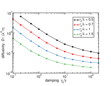
Figure 1: Diffusion constant depending on the solute size $r_{\textnormal{s}}$ and coupling strength $\gamma_{\textnormal{s}}$. Data obtained by simulating system size $L=100\lambda$ at dilute solute density $\rho_{\textnormal{s}}=10^{-3}\lambda^{-3}$ and timestep $\Delta t=10^{-3}\tau$ at the standard DPD parameters: $r_{\textnormal{c}}=\lambda$, $\rho=3r_{\textnormal{c}}^{-3}$, $a_{ij}=78k_{\textnormal{B}}T$, $\gamma=4.5k_{\textnormal{B}}T\tau r_{\textnormal{c}}^{-2}$. $D=\langle r^{2}\rangle/(6\tau)$ with the MSD $\langle r^{2}\rangle$ calculated in the diffusive regime ($t>50\tau$).

The diffusion constant $D=D(r_{\textnormal{s}},\gamma_{\textnormal{s}})$ measured via the mean-squared displacement is shown in Figure 1. The diffusion constant scaling can also be estimated analytically. Strong coupling, $\gamma_{\textnormal{s}}\to\infty$, implies the solvent is rigidly coupled to the solute within range $r_{\textnormal{s}}$, thus the solute behaves as a solid sphere with radius $r_{\textnormal{s}}$ whose diffusivity is given by the Stokes-Einstein relation, $D=k_{\textnormal{B}}T/(6\pi\eta r_{\textnormal{s}})$. Conversely, in the weak coupling regime, the diffusion constant can be calculated by mapping the thermostat forces to a Langevin equation Groot and Warren (1997), which yields the diffusion constant $D=15k_{\textnormal{B}}T/2\pi\gamma_{\textnormal{s}}\rho r_{\textnormal{s}}^{3}$ (note that this expression is a factor 3 smaller than the result in Ref. Groot and Warren (1997) due to inclusion of shear forces, $\gamma_{\perp}=\gamma$). These two limits imply the following functional form for the diffusion constant of the solutes,

$$D(r_{\textnormal{s}},\gamma_{\textnormal{s}})=\frac{k_{\textnormal{B}}T}{2\pi r_{\textnormal{s}}}\left(\frac{1}{3\eta}+\frac{15}{\rho\gamma_{\textnormal{s}}r_{\textnormal{s}}^{2}}\right)\;.$$ (7)

Using this scaling, the simulation data collapse to a master plot and follow Eq. (7) to within $\approx 30\%$ (Fig. 2). Therefore Eq. (7) can be used to estimate $\gamma_{\textnormal{s}}$ given a desired diffusion constant $D$ and solute size $r_{\textnormal{s}}$. If the thermostat without shear forces is used ($\gamma_{\perp,\textnormal{s}}=0$), the second term in Eq. (7) should be multiplied by a factor 3.

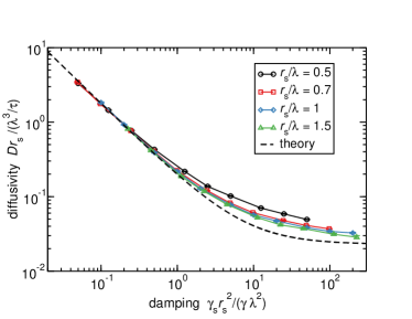
Figure 2: Master plot of diffusivity data from simulations (symbols) and comparison to the analytical prediction (dashed line, Eq. (7)).

The diffusion constant of a typical small solute such as an ion or a small molecule is $D\approx 1~{}\textnormal{nm}^{2}/\textnormal{ns}$, which is $D\approx 0.078\lambda^{2}/\tau$ in the standard DPD units ($\lambda=0.646~{}\textnormal{nm}$, $\tau=0.029~{}\textnormal{ns}$). Our simulation data confirm that chosing the mass of the solute particles the same as the mass of the DPD particles the dynamics are already fully in the diffusive regime at $\langle r^{2}\rangle=\lambda^{2}$ (Fig. 3). As expected, the dynamics do not depend on specific $\gamma_{\textnormal{s}}$ and $r_{\textnormal{s}}$ as long as $D$ is kept constant. The transition from ballistic to diffusive dynamics occurs on the lengtscale $r_{\textnormal{BD}}\sim\sqrt{D\tau}\approx 0.28\lambda$. Therefore, we conclude that the standard DPD friction $\gamma=4.5k_{\textnormal{B}}T\tau r_{\textnormal{c}}^{-2}$ models the appropriate diffusive dynamics on the relevant lengthscales ($r\geq\lambda$).

If necessary, the ballistic–diffusive transition $\tau_{\textnormal{BD}}$ can be pushed to even smaller values by increasing the DPD solvent friction $\gamma$ or decreasing the solute mass, but both would require a smaller integration time-step decreasing the efficiency. Conversely, if a larger ballistic regime is permitted, $\gamma$ could be decreased which would reduce the DPD viscosity and thus increase the value of the time unit $\tau$, allowing exploration of longer timescales, but that would also reduce the Schmidt number (Sc), which may be important, see discussion below.

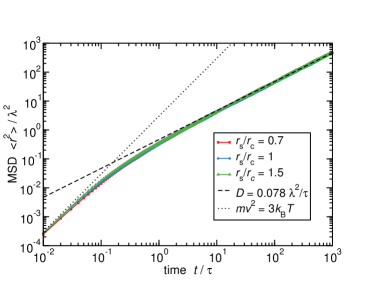
Figure 3: Mean-squared displacement (MSD) of solutes in bulk solution for different $r_{\textnormal{s}}$ at $D\approx 0.078\lambda^{2}/\tau$. [$r_{\textnormal{s}}$, $\gamma_{\textnormal{s}}]=[0.7\lambda,30\gamma]$ (red squares), $[\lambda,5\gamma]$ (blue diamonds), $[1.5\lambda,\gamma]$ (green triangles) showing the ballistic-to-diffusive transition does not explicitly depend on $\gamma_{\textnormal{s}}$ and $r_{\textnormal{s}}$, but only on $D$.

II.1 Limitation of the method: solute permeability

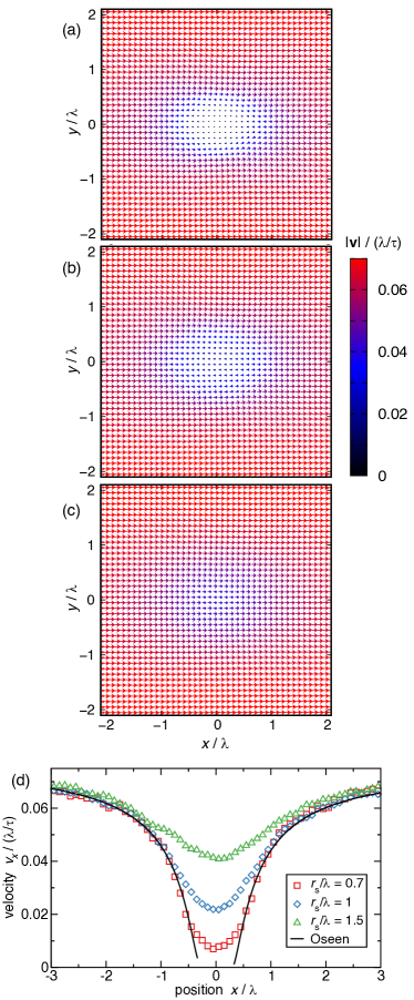
Figure 4: Velocity profile around a spherical solute located at $x=y=z=0$. (a,b,c) The three profiles are obtained at [$r_{\textnormal{s}}$, $\gamma_{\textnormal{s}}]=[0.7\lambda,30\gamma]$ (a), $[\lambda,5\gamma]$ (b), $[1.5\lambda,\gamma]$ (c) corresponding to $D=0.078\lambda^{2}/\tau$ (Fig. 3). The profiles are calculated by averaging the velocity of all DPD particles within $-0.1<z/\lambda<0.1$ for $t=10^{7}\tau$. System size $L=10\lambda$ with periodic boundary conditions and body force density $G_{x}=10^{-3}k_{\textnormal{B}}T/\lambda^{4}$ imposed on DPD particles. (d) The velocity $v_{x}$ on the center line is obtained by averaging within $-0.1<y/\lambda<0.1$ and $-0.1<z/\lambda<0.1$. The Oseen analytical prediction (black line) is given by Eq. (8).

The main limitation of using only the dissipative and random forces for the solute–solvent interaction is that solutes are not impermeable to the solvent particles. The coupling $\gamma_{\textnormal{s}}$ effectively determines the local viscosity at the location of the solute particle, but the solvent can pass through the solute. This is illustrated by the velocity profiles around a spherical solute (Fig. 4). Larger coupling $\gamma_{\textnormal{s}}$ leads to smaller fluid velocity at the particle location. In the limit $\gamma_{\textnormal{s}}\to\infty$ the solute becomes effectively impermeable. In this sense, DPDS bears similarity to the MPC Gompper et al. (2009) and FPD Tanaka and Araki (2000) methods.

The effect of permeability can be systematically investigated by choosing different $r_{\textnormal{s}},\gamma_{\textnormal{s}}$ that yield the desired diffusion constant (Fig. 4). At large $\gamma_{\textnormal{s}}$ the flow profile approaches the Oseen prediction for an impermeable spherical particle Batchelor (1967),

$$v_{x}^{\textnormal{b}} = v_{0}\left(1+\frac{a^{3}}{2x^{3}}-\frac{3a}{2x}\right),$$

$$v_{x}^{\textnormal{f}} = v_{0}\left(1+\frac{a^{3}}{2x^{3}}-\frac{3a^{2}}{2x^{2}\textnormal{Re}}\left[1-e^{-x\textnormal{Re}/a}\right]\right),$$ (8)

where $v_{x}^{\textnormal{b}}$ and $v_{x}^{\textnormal{f}}$ are the flow velocities behind and in front of the particle on the symmetry axis at $z=y=0$. $v_{0}=Df_{\textnormal{particle}}/[k_{\textnormal{B}}T(1+3\textnormal{Re/8})]$ is the far field velocity at total force $f_{\textnormal{particle}}=G_{x}L^{3}$ with $G_{x}$ the body force on the fluid and $L$ the system size (to calculate the flow profiles the particle is immobilized and the force is applied on the fluid). The radius of a sphere that yields the desired diffusion constant $D$ is $a=k_{\textnormal{B}}T/(6\pi\eta D)$ and the corresponding Reynolds number $\textnormal{Re}=a\rho v_{0}/\eta$. The simulated flow profiles approach the Oseen prediction for large $\gamma_{\textnormal{s}}$ (Fig. 4d). The ratio $\gamma_{\textnormal{s}}/\gamma=5$ appears to be sufficiently large to reproduce the Oseen profile to a distance $r\approx 3/4\lambda$ and also the hydrodynamic scaling of polymer collapse as shown below.

If full blocking of the solute is required, repulsive interactions between solute and solvent can be added to the model, but the resulting solvent–solute depletion interactions must taken into account, which likely requires reparametrization of solute–solute interactions.

II.2 Recipe

We provide a straightforward recipe on how to use the DPDS method with coarse-grained models of solutes.

1. Choose the desired solvent properties: determine the minimum DPD length scale $r_{\textnormal{c}}$ on which to resolve hydrodynamics and obtain the desired compressibility via $a_{ij}$ Groot and Warren (1997). Chose the thermostat coupling $\gamma$ that results in the desired transition between ballistic and diffusive regimes. The standard parameters, $r_{\textnormal{c}}=0.646~{}$nm, $\rho=3r_{\textnormal{c}}^{-3}$, $a_{ij}=78k_{\textnormal{B}}T$, $\gamma=4.5\sqrt{k_{\textnormal{B}}Tm}/r_{\textnormal{c}}$ are likely a good starting point for most coarse-grained models of aqueous solutions of molecules, ions, and polymers.

2. Determine the solute–solvent coupling, $r_{\textnormal{s}}$ and $\gamma_{\textnormal{s}}$ that yield the desired solute diffusivity $D$: The size $r_{\textnormal{s}}$ should be similar to the physical size of the solutes and $\gamma_{\textnormal{s}}$ is determined via Eq. (7) or by measuring the mean-squared displacement of solutes.

This introduces both hydrodynamics interactions and thermostating of the solute system, while maintaining the equilibrium configurational distribution of the solutes. An example implementation in the open-source MD package LAMMPS is provided in the Appendix.

III Applications

To demonstrate the applicability of the DPDS method, we investigate two different systems where hydrodynamic interactions play a crucial role: the collapse and diffusion dynamics of a single polymer and electroosmotic flow of an electrolyte solution.

III.1 Polymer dynamics

We consider a bead–spring polymer model Stevens and Kremer (1995) in an aqueous solution. Consecutive beads in a polymer chain of $N$ beads are connected via a harmonic potential

$$U=\frac{K}{2}(r_{ij}-\lambda)^{2}$$ (9)

with zero-energy bond length $\lambda$ and strength $K=100k_{\textnormal{B}}T/\lambda^{2}$.

The polymer is immersed in a DPD solvent described by the standard parameters for an aqueous solution ($\rho=3r_{\textnormal{c}}^{-3}$, $\gamma=4.5k_{\textnormal{B}}T\tau/r_{\textnormal{c}}^{2}$, $a_{ij}=78k_{\textnormal{B}}T$, $r_{\textnormal{c}}=\lambda=0.646$ nm). The coupling between the polymer beads and the DPD fluid is achieved with $\gamma_{\textnormal{s}}=5\gamma$ and $r_{\textnormal{s}}=r_{\textnormal{c}}$, which models the diffusion constant of individual monomers $D=1.1~{}\textnormal{nm}^{2}/\textnormal{ns}$ (cf. Fig. 1). The system is evolved using the velocity-Verlet integrator with time step $\Delta t=0.005\tau$.

First, we measure the diffusion constant for different polymer sizes and compare the scaling with the Zimm dynamics prediction $D\propto N^{-\nu}$, with $\nu$ the scaling exponent. At good-solvent conditions $\nu=0.588$ Rubinstein and Colby (2003). The system is a cubic box with size $L=100\lambda$ and periodic boundary conditions. Polymers of length $N$ and monomer density $\rho_{\textnormal{m}}=10^{-3}/\lambda^{3}$ are equilibrated at good solvent conditions. Bead–bead repulsion is modeled as a Lennard-Jones (WCA) interaction with size $\sigma=\lambda$, strength $\varepsilon={k_{\textnormal{B}}T}$ and cutoff $r_{\textnormal{cut}}=2^{1/6}\sigma$. We measure the mean-squared-displacement of all monomers $\langle r^{2}\rangle$ for $t=5000\tau$. The diffusion constant is measured via the slope of the average mean squared-displacement as a function of time, $6D=\partial\langle r^{2}\rangle/\partial t$; at large displacements, $\langle r^{2}\rangle>(2R_{\textnormal{g}})^{2}$.

The scaling of the diffusion constant with size fully reproduces the expected Zimm dynamics (Fig. 5). Small deviations ($<10\%$) occur for very short polymers ($N\sim 1$) due to finite size effects.

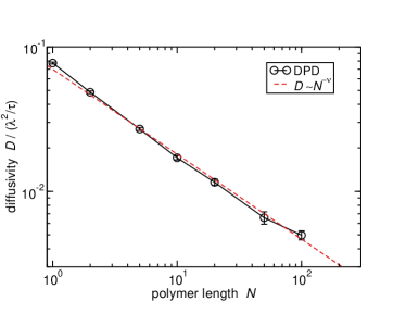
Figure 5: Diffusion constant $D$ dependence on polymer size $N$. Simulation data (black circles) is well described by Zimm dynamics (red dashed line) with the good-solvent scaling exponent $\nu=0.588$. Error bars denote standard errors obtained from 8 independent simulations.

We next measure the timescale of a hydrophobic collapse of the polymer, a problem related to the dynamics of protein folding. Analytical predictions for the hydrophobic collapse timescale $\tau_{\textnormal{c}}$ of an initially expanded polymer indicate $\tau_{\textnormal{c}}\sim N^{2}$ for brownian dynamics and $\tau_{\textnormal{c}}\sim N^{4/3}$ with hydrodynamics Kikuchi et al. (2005), since a polymer globule needs to travel a distance $\sim N$ while the drag on the collapsed globules scales as $\sim N$ for brownian dynamics and $\sim N^{1/3}$ for Stokes flow.

The collapse timescale $\tau_{\textnormal{c}}$ is defined by the time required for the change in the radius of gyration $R_{\textnormal{g}}(t)$ to reach a fraction $f_{\textnormal{c}}=0.9$ of the maximum change,

$$R_{\textnormal{g}}(\tau_{\textnormal{c}})=(1-f_{\textnormal{c}})R_{\textnormal{g,0}}+f_{\textnormal{c}}R_{\textnormal{g,col}}\;,$$ (10)

where $R_{\textnormal{g,0}}$ and $R_{\textnormal{g,col}}$ are, respectively, the initial and the final (collapsed) $R_{\textnormal{g}}$ values. We consider two initial configurations, (i) a fully expanded linear polymer ($R_{\textnormal{g},0}\sim N$) and (ii) a polymer equilibrated at good solvent conditions ($R_{\textnormal{g},0}\sim N^{\nu}$) with the scaling exponent $\nu=0.588$ Rubinstein and Colby (2003). To model the collapse, we introduce attractive interactions between monomers modeled by the Lennard-Jones potential with size $\sigma=\lambda$, strength $\varepsilon=1.25k_{\textnormal{B}}T$, and cutoff $r_{\textnormal{LJcut}}=2.5\sigma$. Simulation data shown in Fig. 6 show the scaling follows $\tau_{\textnormal{c}}\sim N^{1.42\pm 0.02}$ for an initially fully stretched polymer, while $\tau_{\textnormal{c}}\sim N^{0.95\pm 0.04}$ for an initially equilibrated polymer. This scaling is close to the analytical prediction for an expanded polymer $N^{4/3}$ and agrees with the DPD predictions for an equilibrated polymer $N^{0.98\pm 0.09}$ Guo et al. (2011).

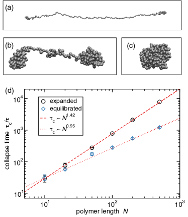
Figure 6: Polymer collapse. (a,b,c) configurations of a bead-spring polymer of size $N=200$ during collapse from an initially fully-expanded linear chain at (a) $t=500\tau$, (b) $t=2000\tau$, and (c) $t=2500\tau$. (d) DPD simulation data showing collapse timescale dependence on the polymer size $N$ for an initially expanded linear chain (circles), which follows $\sim N^{1.42\pm 0.02}$ scaling, and an initially equilibrated polymer at good solvent conditions (diamonds), which follows $\sim N^{0.95\pm 0.05}$. System size for initially expanded case, $L_{x}=N+10\lambda$, $L_{y}=L_{z}=50\lambda$, and for equilibrated polymers $L_{x}=L_{y}=L_{z}=80\lambda$. Error bars denote standard errors obtained from 5 (black circles) and 20 (blue diamonds) independent simulations.

This data on polymer diffusion and collapse timescale indicate that the proposed method faithfully reproduces the hydrodynamic coupling between a polymer and solvent.

III.2 Nanochannel flow

We next consider the electro-osmotic flow of an electrolyte solution in a slit nanochannel and investigate the coupling between hydrodynamics and electrostatic interactions. To use DPDS for wall-bounded flows, we must first briefly discuss a method to impose a desired no-slip or slip boundary condition at the channel walls.

III.2.1 wall boundary condition

To impose the desired boundary condition at the channel walls, we investigate a pure solvent system without ions. Implementation of solid walls within DPD simulations is not straightforward due to layering artifacts that can occur next to a flat wall Pivkin and Karniadakis (2005). A no-slip boundary condition can be imposed by introducing a layer of immobilized DPD particles at the walls Barcelos et al. (2021), however, due to repulsive interactions, the slip length dependence on the wall particle density is non-monotonic. Another possibility is to impose a drag force parallel to the wall Smiatek et al. (2008, 2009).

Here we propose an alternative strategy to impose a boundary condition by coupling the DPD fluid to the immoblized wall particles only through the thermostat with coupling strength $\gamma_{\textnormal{w}}$, which is determined by the desired slip-length. The method is very similar to using a parallel drag force Smiatek et al. (2008), but is expected to be easier to employ because it does not require a separate implantation of a wall–DPD thermostat.

The DPD solvent particles interact with a smooth repulsive surface via a repulsive WCA interaction with $\sigma=r_{\textnormal{c}}$ and $\varepsilon=k_{\textnormal{B}}T$. The smooth repulsive surfaces are positioned at $y_{\textnormal{wall}}=\pm(w/2+r_{\textnormal{c}})$, where $w$ is the width of the nanochannel. In addition, immobile particles are placed at the wall surface $y_{\textnormal{im}}=\pm w/2$, at 2D density $\rho_{\textnormal{w}}=\rho r_{\textnormal{c}}$ arranged on a regular mesh with lattice spacing $a_{\textnormal{w}}=\rho_{\textnormal{w}}^{-1/2}$. These immobile particles interact with the DPD particles only via the DPD thermostat with strength $\gamma_{\textnormal{w}}$ and range $r_{\textnormal{c}}$ [Eqs. 2, 3, 5].

To induce flow, a pressure gradient $G_{x}$ is imposed on the fluid as a body force, $f_{x}=G_{x}/\rho$, which acts on each DPD particle. The system size is $L_{y}=L_{z}=w$ and $L_{x}=40\lambda$ with periodic boundary conditions in $x$ and $z$. The system is simulated for $t_{\textnormal{init}}=5000\tau$ to reach steady state followed by $t=5\cdot 10^{5}\tau$ for calculation of the velocity profiles at different values of the wall–solvent coupling $\gamma_{\textnormal{w}}$ (Fig. 7).

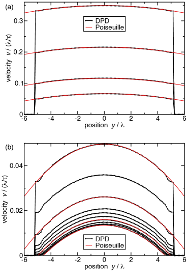
Figure 7: Velocity flow profile from DPD simulations (black circles) and comparison to Poiseuille profiles (red curves) given by Eq. (11). (a,b) DPD data (black) from bottom to top are obtained at $\gamma_{\textnormal{w}}/\gamma=[5,3,2,1,0.5,0.3,0.2,0.1,0.05,0.03,0.02,0.01,0.005]$ at pressure gradient $G_{x}=0.003k_{\textnormal{B}}T/\lambda$ and $w=10\lambda$. Poiseuille prediction (red curves) from bottom to top shown for slip length $L_{\textnormal{s}}/\lambda=[-0.42,-0.03,1.52,5.15,7.7,15.3,30.7,51.2]$ at viscosity $\eta=2.31k_{\textnormal{B}}T\tau/\lambda^{3}$ [Eq. (11)].

The velocity profile between two parallel plates at low Reynolds numbers follows the parabolic Poiseuile profile,

$$v(y)=\frac{G_{x}}{2\eta}(w^{2}/4-y^{2}+wL_{\textnormal{s}}).$$ (11)

The slip length

$$L_{\textnormal{s}}=\pm{\Delta v}\left[\left(\frac{\partial v}{\partial y}\right)_{y=\mp w/2}\right]^{-1}\;,$$ (12)

is determined by the slip velocity $\Delta v$ at the wall. We find the simulated velocity profiles accurately reproduce the parabolic Poiseuille profiles for at least two orders of magnitude in flow velocity and slip lengths from zero to larger than channel width (Fig. 7). A small deviation from the parabolic profile is observed within a distance $r_{\textnormal{c}}$ of the wall due to the layering effect of the DPD particles next to a smooth repulsive wall.

To avoid numerical errors when calculating derivatives [Eq. (12)], we determine the slip length from averages in the velocity. Since the velocity profiles are parabolic (Fig. 7), the slip length can be obtained by integrating the profile [Eq. (11)],

$$L_{\textnormal{s}}=\left(\frac{\bar{v}}{\bar{v}_{\textnormal{P}}}-1\right)\frac{w}{6}$$ (13)

where $\bar{v}$ is the average velocity in the channel and

$$\bar{v}_{\textnormal{P}}=\frac{G_{x}w^{2}}{12\mu}$$ (14)

is the average velocity for Poiseuille profile at $L_{\textnormal{s}}=0$. Thus, we obtain the slip length as a function of wall damping $\gamma_{\textnormal{w}}$ (Fig. 8).

Analytical considerations show that to second order the slip length is given by

$$L_{\textnormal{s}}/r_{\textnormal{c}}=c_{1}/\alpha-c_{2}-\mathcal{O}(\alpha)$$ (15)

with $\alpha=r_{\textnormal{c}}^{2}\gamma_{\textnormal{w}}\rho/\eta$ Smiatek et al. (2008) and the positive constants $c_{1},c_{2}$ of order unity that depend on the wall solvent interaction. We find that fitting $c_{1}=0.9$ and $c_{2}=0.13$ can be used to predict $L_{\textnormal{s}}$ to accuracy within $0.1r_{\textnormal{c}}$ (Fig. 8).

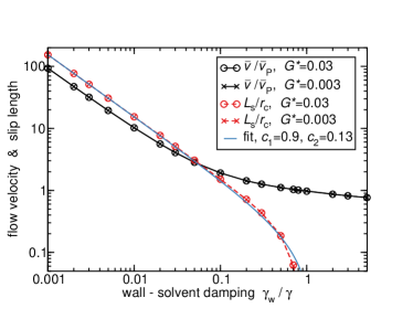
Figure 8: Average velocity obtained from simulations (solid black line) and corresponding slip length using Eq. (13) (dashed red lines) using viscosity $\eta=2.31k_{\textnormal{B}}T\tau/\lambda^{3}$. The data for different pressure gradients $G^{*}=G_{x}/k_{\textnormal{B}}T\rho\lambda$ show perfect overlap. The two parameter fit [Eq. (15)](solid blue line) is accurate to within $0.1r_{\textnormal{c}}$.

III.2.2 electroosmotic flow

Having described the channel setup and the wall interaction, we show how to simulate hydrodynamic flow of an electrolyte. Free monovalent ions are modeled as charged spheres with the short-range ion–ion repulsion modeled by the WCA potential with hydrated ion diameter $\sigma=\lambda=0.646~{}\textnormal{nm}$, and interaction strength $\varepsilon=k_{\textnormal{B}}T$. The experimentally measured value for small-ion diffusivity, $D\approx\textnormal{nm}^{2}/\textnormal{ns}$, is obtained at solvent–solute coupling strength $\gamma_{\textnormal{s}}=5\gamma$ and range $r_{\textnormal{s}}=\lambda$ (cf. Fig. 3). The electrostatic interactions are calculated using PPPM Ewald summation with real-space cutoff $r_{\textnormal{ewald}}=5\lambda$ and relative force accuracy of $10^{-4}$. Slab correction factor 3.0 is used in the $y$ coordinate to simulate fixed boundary conditions at the channel walls. Electrostatic strength is determined by the Bjerrum length $l_{\textnormal{B}}=0.71\,$nm corresponding to an aqueous solution at room temperature.

We consider an electroosmotic flow in a nanochannel of width $w=8\lambda$ under an external electric field $E_{x}$. To investigate a non-symmetric case where accurate description of convection and diffusion of ions is important, the wall contains a small charged section that covers a fraction $f_{\textnormal{w}}=0.25$ of the wall surface with charge density $\sigma_{\textnormal{q}}=0.2e_{0}/\lambda^{2}$ (see Fig. 9a). The solution contains counter-ions at density $\rho_{\textnormal{ion}}=2\sigma_{\textnormal{q}}f_{\textnormal{w}}/w$. This configuration introduces a pattern in the charge density and Poisson-Boltzmann (PB) calculations predict two distinct regimes due to the localization of counter-ions at small external fields Curk et al. (2024). This effect is pronounced at non-zero slip lengths and we use $L_{\textnormal{s}}=30\lambda$, a typical order of magnitude for a slip length of an aqueous solution Joseph and Tabeling (2005).

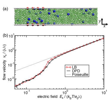
Figure 9: electroosmotic flow in a slit channel. (a) Configuration setup showing DPD particles (green), immobile wall particles (white), surface charge (red), and counterions in (blue). (b) Mean velocity in a slit channel obtained from DPD simulations and comparison to lattice-Boltzmann (LB) and Poiseuille prediction [Eq. (14)] at driving force $G_{x}=E_{x}e_{0}\rho_{\textnormal{ion}}$. Slip length $L_{\textnormal{s}}\approx 30\lambda$ is obtained at $\gamma_{\textnormal{w}}=0.005\gamma$ in DPD, and fractional bounce-back $f_{\textnormal{bb}}=0.99$ in LB.

The DPDS results are in an excellent agreement with PB simulations and clearly show two distinct flow regimes (Fig. 9). The PB calculations are performed by employing the Ludwig open-source package with electrokinetics Capuani et al. (2004) using lattice size $\Delta x=\lambda/2$, reduced viscosity $\eta^{*}=0.2$ and parameters corresponding to kinematic viscosity of water $\nu=10^{-6}~{}\textnormal{m}^{2}/\textnormal{s}$. The desired slip length is obtained via a fractional bounce-back boundary condition Wolff et al. (2012) with fraction $f_{\textnormal{bb}}$. All other parameters are the same as described for DPD. Small deviations between DPD and PB occur at the transition between the two flow regimes, which we attribute to the lack of thermal fluctuations in the PB model, as well as the lattice approximation and the associated lack of unit charge discretization in PB. However, the flow velocity in the two regimes is in perfect agreement.

IV summary

In summary, we proposed a DPD-solvent (DPDS) method that introduces solvent hydrodynamics to coarse-grained models of solutes. The solute–solvent interaction occurs only via the dissipative and random forces, which ensures the equilibrium configurational properties of the solute system are not affected by the presence of the DPD solvent. The solute–solvent coupling strength is determined by the desired diffusion constants of the solute. Because the method is based on short-ranged DPD interactions, the computational cost scales linearly with the system size Frenkel and Smit (2002).

The DPDS method can be utilized as a replacement for a Nosé-Hoover or Langevin thermostat in coarse-grained MD simulations, while capturing the hydrodynamic interactions at desired solvent compressibility, viscosity and solute diffusivity (see Recipe section). The examples shown demonstrate the method reproduces the correct hydrodynamic of Oseen flow, channel flow, electroosmotic effects, and polymer hydrodynamics. Moreover, since the method utilizes the standard DPD thermostat, the simulations can be performed using existing implementations in open-source molecular dynamics packages such as LAMMPS and ESPResSo. Thus, the method should be broadly useful as means to introduce hydrodynamics to existing coarse-grained models of molecules and soft materials.

The method could be used with multicomponent solvents that are described by two or more different types of DPD particles Pagonabarraga and Frenkel (2001); Merabia et al. (2008). In this case, the solute–solvent coupling could be distinct among different solvents, modeling different diffusivities. In addition, the chemical potential difference of the solutes in different solvents could be introduced by soft solute–solvent interactions. While we have only considered solute models based on spherical excluded-volume interactions, such as ions or monomers in a polymers, the method can be applied to non-spherically symmetric solutes, for example, by uniformly distributing ghost particles inside a non-spherical object and coupling these ghost particles to the DPD solvent via Eqs. (2) and (3).

*

Appendix A A

Implementation of the DPD-solvent in the LAMMPS open-source MD package can be achieved using the existing dpd or dpd/ext pair styles Thompson et al. (2022). Let us assume that type 1 is the solvent and type 2 is the solute. For the solute–solvent, polymer–solvent and ion–solvent interaction cases discussed in Sec. II and III (using the LJ reduced units with unit length $\lambda=r_{\textnormal{c}}=1$ and DPD particle density $\rho=3\lambda^{-3}$), the solvent properties are determined by the DPD model:

pair_coeff 1 1 dpd/ext $a_{ij}$ $\gamma$ $\gamma_{\perp}$ 1 1 1

while the solute–solvent coupling is determined by the thermostat:

pair_coeff 1 2 dpd/ext/tstat $\gamma_{\textnormal{s}}$ $\gamma_{\perp,\textnormal{s}}$ 1 1 $r_{\textnormal{s}}/\lambda$

Combining these instructions with the desired solute–solute interactions and a velocity-Verlet integrator introduces hydrodynamic interactions without affecting the equilibrium canonical distribution of the solute particles as compared to using a Langevin or Nosé-Hoover thermostat.

References

- Malevanets and Kapral (1999) A. Malevanets and R. Kapral, The Journal of Chemical Physics 110, 8605 (1999), ISSN 0021-9606, eprint https://pubs.aip.org/aip/jcp/article-pdf/110/17/8605/10798234/8605_1_online.pdf, URL https://doi.org/10.1063/1.478857.
- Gompper et al. (2009) G. Gompper, T. Ihle, D. M. Kroll, and R. G. Winkler, Multi-Particle Collision Dynamics: A Particle-Based Mesoscale Simulation Approach to the Hydrodynamics of Complex Fluids (Springer Berlin Heidelberg, Berlin, Heidelberg, 2009), pp. 1–87, ISBN 978-3-540-87706-6, URL https://doi.org/10.1007/978-3-540-87706-6_1.
- Krueger et al. (2016) T. Krueger, H. Kusumaatmaja, A. Kuzmin, O. Shardt, G. Silva, and E. M. Viggen, The Lattice Boltzmann Method: Principles and Practice, Graduate Texts in Physics (Springer, 2016), ISBN 978-3-319-44647-9.
- Tanaka and Araki (2000) H. Tanaka and T. Araki, Phys. Rev. Lett. 85, 1338 (2000).
- Dünweg and Ladd (2009) B. Dünweg and A. J. C. Ladd, Lattice Boltzmann Simulations of Soft Matter Systems (Springer Berlin Heidelberg, Berlin, Heidelberg, 2009), pp. 89–166, ISBN 978-3-540-87706-6, URL https://doi.org/10.1007/978-3-540-87706-6_2.
- Furukawa et al. (2018) A. Furukawa, M. Tateno, and H. Tanaka, Soft Matter 14, 3738 (2018), URL http://dx.doi.org/10.1039/C8SM00189H.
- Soddemann et al. (2003) T. Soddemann, B. Dünweg, and K. Kremer, Phys. Rev. E 68, 046702 (2003), URL https://link.aps.org/doi/10.1103/PhysRevE.68.046702.
- Hoogerbrugge and Koelman (1992) P. J. Hoogerbrugge and J. M. V. A. Koelman, Europhysics Letters 19, 155 (1992), URL https://dx.doi.org/10.1209/0295-5075/19/3/001.
- Groot and Warren (1997) R. D. Groot and P. B. Warren, The Journal of Chemical Physics 107, 4423 (1997), URL https://doi.org/10.1063/1.474784.
- Espa ol and Warren (2017) P. Espanol and P. B. Warren, The Journal of Chemical Physics 146, 150901 (2017), ISSN 0021-9606, eprint https://pubs.aip.org/aip/jcp/article-pdf/doi/10.1063/1.4979514/14899131/150901_1_online.pdf, URL https://doi.org/10.1063/1.4979514.
- Pagonabarraga and Frenkel (2001) I. Pagonabarraga and D. Frenkel, The Journal of Chemical Physics 115, 5015 (2001), ISSN 0021-9606, eprint https://pubs.aip.org/aip/jcp/article-pdf/115/11/5015/10834712/5015_1_online.pdf, URL https://doi.org/10.1063/1.1396848.
- Groot and Rabone (2001) R. Groot and K. Rabone, Biophysical Journal 81, 725 (2001), ISSN 0006-3495, URL https://www.sciencedirect.com/science/article/pii/S0006349501757372.
- Groot (2003) R. D. Groot, The Journal of Chemical Physics 118, 11265 (2003), ISSN 0021-9606, eprint https://pubs.aip.org/aip/jcp/article-pdf/118/24/11265/10849245/11265_1_online.pdf, URL https://doi.org/10.1063/1.1574800.
- Junghans et al. (2008) C. Junghans, M. Praprotnik, and K. Kremer, Soft Matter 4, 156 (2008), URL http://dx.doi.org/10.1039/B713568H.
- Pagonabarraga et al. (1998) I. Pagonabarraga, M. H. J. Hagen, and D. Frenkel, Europhysics Letters 42, 377 (1998), URL https://dx.doi.org/10.1209/epl/i1998-00258-6.
- Santo and Neimark (2021) K. P. Santo and A. V. Neimark, Advances in Colloid and Interface Science 298, 102545 (2021), ISSN 0001-8686, URL https://www.sciencedirect.com/science/article/pii/S000186862100186X.
- Lauriello et al. (2021) N. Lauriello, J. Kondracki, A. Buffo, G. Boccardo, M. Bouaifi, M. Lisal, and D. Marchisio, Physics of Fluids 33, 073106 (2021), ISSN 1070-6631, URL https://doi.org/10.1063/5.0055344.
- Spenley (2000) N. A. Spenley, Europhysics Letters 49, 534 (2000), URL https://dx.doi.org/10.1209/epl/i2000-00183-2.
- Krafnick and Garc a (2015) R. C. Krafnick and A. E. Garcia, The Journal of Chemical Physics 143, 243106 (2015), ISSN 0021-9606, eprint https://pubs.aip.org/aip/jcp/article-pdf/doi/10.1063/1.4930921/15506986/243106_1_online.pdf, URL https://doi.org/10.1063/1.4930921.
- Lowe, C. P. (1999) Lowe, C. P., Europhys. Lett. 47, 145 (1999), URL https://doi.org/10.1209/epl/i1999-00365-x.
- Boromand et al. (2015) A. Boromand, S. Jamali, and J. M. Maia, Computer Physics Communications 196, 149 (2015), ISSN 0010-4655, URL https://www.sciencedirect.com/science/article/pii/S0010465515002076.
- Stevens and Kremer (1995) M. J. Stevens and K. Kremer, J. Chem. Phys. 103, 1669 (1995).
- Marrink et al. (2007) S. J. Marrink, H. J. Risselada, S. Yefimov, D. P. Tieleman, and A. H. de Vries, The Journal of Physical Chemistry B 111, 7812 (2007), ISSN 1520-6106, URL https://doi.org/10.1021/jp071097f.
- Snodin et al. (2015) B. E. K. Snodin, F. Randisi, M. Mosayebi, P. Šulc, J. S. Schreck, F. Romano, T. E. Ouldridge, R. Tsukanov, E. Nir, A. A. Louis, et al., The Journal of Chemical Physics 142, 234901 (2015), ISSN 0021-9606, eprint https://pubs.aip.org/aip/jcp/article-pdf/doi/10.1063/1.4921957/15496870/234901_1_online.pdf, URL https://doi.org/10.1063/1.4921957.
- Batchelor (1967) G. K. Batchelor, An introduction to Fluid dynamics (Cambridge University Press, Berlin, Heidelberg, 1967).
- Rubinstein and Colby (2003) M. Rubinstein and R. H. Colby, Polymer Physics, vol. 23 (Oxford university press New York, 2003).
- Kikuchi et al. (2005) N. Kikuchi, J. F. Ryder, C. M. Pooley, and J. M. Yeomans, Phys. Rev. E 71, 061804 (2005), URL https://link.aps.org/doi/10.1103/PhysRevE.71.061804.
- Guo et al. (2011) J. Guo, H. Liang, and Z.-G. Wang, The Journal of Chemical Physics 134, 244904 (2011), ISSN 0021-9606, eprint https://pubs.aip.org/aip/jcp/article-pdf/doi/10.1063/1.3604812/15440872/244904_1_online.pdf, URL https://doi.org/10.1063/1.3604812.
- Pivkin and Karniadakis (2005) I. V. Pivkin and G. E. Karniadakis, Journal of Computational Physics 207, 114 (2005), ISSN 0021-9991, URL https://www.sciencedirect.com/science/article/pii/S0021999105000197.
- Barcelos et al. (2021) E. I. Barcelos, S. Khani, A. Boromand, L. F. Vieira, J. A. Lee, J. Peet, M. F. Naccache, and J. Maia, Computer Physics Communications 258, 107618 (2021), ISSN 0010-4655, URL https://www.sciencedirect.com/science/article/pii/S0010465520302964.
- Smiatek et al. (2008) J. Smiatek, M. P. Allen, and F. Schmid, The European Physical Journal E 26, 115 (2008), ISSN 1292-895X, URL https://doi.org/10.1140/epje/i2007-10311-4.
- Smiatek et al. (2009) J. Smiatek, M. Sega, C. Holm, U. D. Schiller, and F. Schmid, The Journal of Chemical Physics 130, 244702 (2009), ISSN 0021-9606, eprint https://pubs.aip.org/aip/jcp/article-pdf/doi/10.1063/1.3152844/15996382/244702_1_online.pdf, URL https://doi.org/10.1063/1.3152844.
- Curk et al. (2024) T. Curk, S. G. Leyla, and I. Paganobarraga, ArXiv preprint: arXiv:2401.03666 (2024).
- Joseph and Tabeling (2005) P. Joseph and P. Tabeling, Phys. Rev. E 71, 035303 (2005), URL https://link.aps.org/doi/10.1103/PhysRevE.71.035303.
- Capuani et al. (2004) F. Capuani, I. Pagonabarraga, and D. Frenkel, The Journal of Chemical Physics 121, 973 (2004), URL https://doi.org/10.1063/1.1760739.
- Wolff et al. (2012) K. Wolff, D. Marenduzzo, and M. E. Cates, Journal of The Royal Society Interface 9, 1398 (2012), URL https://royalsocietypublishing.org/doi/abs/10.1098/rsif.2011.0868.
- Frenkel and Smit (2002) D. Frenkel and B. Smit, Understanding Molecular Simulation (Academic, San Diego, 2002), 2nd ed.
- Merabia et al. (2008) S. Merabia, J. Bonet-Avalos, and I. Pagonabarraga, Journal of Non-Newtonian Fluid Mechanics 154, 13 (2008), ISSN 0377-0257, URL https://www.sciencedirect.com/science/article/pii/S0377025708000116.
- Thompson et al. (2022) A. P. Thompson, H. M. Aktulga, R. Berger, D. S. Bolintineanu, W. M. Brown, P. S. Crozier, P. J. in ’t Veld, A. Kohlmeyer, S. G. Moore, T. D. Nguyen, et al., Computer Physics Communications 271, 108171 (2022), ISSN 0010-4655, URL https://www.sciencedirect.com/science/article/pii/S0010465521002836.