Learning-Based Difficulty Calibration for Enhanced
Membership Inference Attacks
Abstract
Machine learning models, in particular deep neural networks, are currently an integral part of various applications, from healthcare to finance. However, using sensitive data to train these models raises concerns about privacy and security. One method that has emerged to verify if the trained models are privacy-preserving is Membership Inference Attacks (MIA), which allows adversaries to determine whether a specific data point was part of a model’s training dataset. While a series of MIAs have been proposed in the literature, only a few can achieve high True Positive Rates (TPR) in the low False Positive Rate (FPR) region (). This is a crucial factor to consider for an MIA to be practically useful in real-world settings. In this paper, we present a novel approach to MIA that is aimed at significantly improving TPR at low FPRs. Our method, named learning-based difficulty calibration for MIA (LDC-MIA), characterizes data records by their hardness levels using a neural network classifier to determine membership. The experiment results show that LDC-MIA can improve TPR at low FPR by up to 4x compared to the other difficulty calibration based MIAs. It also has the highest Area Under ROC curve (AUC) across all datasets. Our method’s cost is comparable with most of the existing MIAs, but is orders of magnitude more efficient than one of the state-of-the-art methods, LiRA, while achieving similar performance.
1 Introduction
Machine learning has become increasingly important in many mission-critical domains, such as healthcare, finance, manufacturing, and cybersecurity. However, these applications often rely on the use of sensitive data as the training dataset for ML models. For instance, large-scale medical images containing private patient information are used to train CNN models for the recognition of body organs [38] and brain tumor segmentation [10]. Another example is that Fu et al. trained a CNN model using real credit card transaction data from a commercial bank to detect fraudulent behaviors [9]. While machine learning has proven to be highly effective in these domains, researchers have cautioned that overfitting can lead to the memorization of training data, potentially resulting in the leakage of sensitive information. To this end, Membership Inference Attacks (MIA) have been developed to determine whether a target sample belongs to the training dataset of a target model.
In most MIAs, the attackers take advantage of the fact that the target model produces more accurate results on the data records in their training dataset compared to those drawn from the same distribution but not included in the training dataset [32, 39, 29]. Shokri et al. proposed training a shadow model to mimic the behavior of the target model by learning from the output of the shadow model when exposed to member and non-member data records [32]. Later, Yeom et al. discovered that an attacker can calculate a membership score, such as the entropy loss value, of a target sample from the target model and use a threshold to determine membership [39]. However, previous works [37, 3, 24] point out that the score-based approach fails to distinguish between members and non-members with high precisions when the non-member data records also have low loss values.
To tackle this issue, Watson et al. proposed the use of a reference model [37], which is an additional model trained on data drawn from the same distribution as those in the training dataset of the target model. Then, each target data record is fed into both the target and reference models to obtain a loss value, respectively. By calculating the difference between the two loss values, the reference model helps calibrate the target model’s behavior on a data record. This approach is an example of a difficulty calibration-based attack, which is currently one of the most advanced MIAs. To further improve the attack performance, Carlini et al. designed a Likelihood Ratio Attack (LiRA) [3]. LiRA utilizes multiple shadow models to estimate the distribution of loss values on a target data record for models that are either trained or not trained on this data sample. Although LiRA achieves high True Positive Rates (TPRs) at low False Positive Rates (FPRs), it requires significant computation.
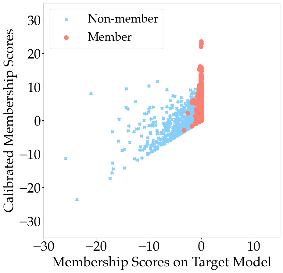
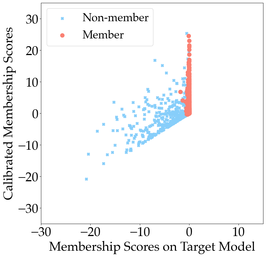
Our proposed attack111The implementation of LDC-MIA is available at https://github.com/horanshi/LDC-MIA is motivated by these works and aims to achieve high TPRs at low FPRs while minimizing the cost for attackers. We consider two types of costs in our attack: the training cost and the data cost. The training cost is mainly dependent on the number of attacking models and their complexities, while the data cost involves the amount of data needed to train the attacking models. We strive to minimize both in our design. In our proposed attack, we also use a reference model. However, unlike other methods, we take into account the intrinsic characteristics of the target data records when calibrating the difficulty of a target data record. Furthermore, we argue that the hardness levels of data records are not universal across different classes because of their distinct data distributions. To illustrate this, we provide an example in Figure 1. The figure shows data records belonging to different classes, Airplane and Cat, the data records are from CIFAR-10 dataset[18]. Each record is represented by a marker that indicates its membership type, while its calibrated membership score is shown on the y-axis, and its membership score on the target model is shown on the x-axis. The calibrated membership score is calculated by taking the difference between a data record’s membership score on the target model and the reference model, as proposed by Watson et al. [37].
Based on the figure, we can make a few important observations. First, the calibrated membership score increases the gap between the easy-to-predict non-members and hard-to-predict members. However, it also reduces the gap between easy-to-predict non-members and hard-to-predict non-members since both groups may have low calibrated membership scores. However, the membership scores along the axis can help easily differentiate between these two groups. Second, it is evident that the two classes have different optimal thresholds for the calibrated membership scores. This indicates that the hardness levels of data records are not universal across different classes. Therefore, it is necessary to adopt a more intelligent approach to determining the threshold values. Third, the data distribution also plays an important role in determining how hard it is for a data record to be classified, in addition to the intrinsic characteristics of data records. As revealed by Long et al. [24], the more neighbors a data record has in the training dataset, the easier it is for it to be correctly classified. This also means that the data record is more likely to be determined as a member by attackers.
Based on these observations, we propose developing a classifier that can learn to calibrate difficulty based on the membership score on the target model, the calibrated membership score, the label of the target data record, and its neighborhood information. To train this classifier, we can use a shadow target model and a reference model trained with data records that share the same distribution as those belonging to the target model training dataset. The shadow target model would mimic the target model’s behavior in classifying members and non-members. We call the proposed attack LDC-MIA. The main contributions of this paper are threefold. (1) The proposed attack significantly improves the TPR at low FPR while minimizing the cost for attackers. We only require one shadow model and one reference model to improve the TPR. Additionally, the classifier we build is a simple model that has three fully connected layers. (2) We conduct a comprehensive characterization of the data records’ hardness levels and use these characters to train a neural network for determining membership. This learning-based calibration approach can be easily extended to integrate other features without requiring significant retraining efforts. (3) Through extensive evaluations, we provide insights into the contributions each of the characters makes to the success of our proposed attack.
We conduct extensive experiments to evaluate the performance of LDC-MIA on various datasets. Specifically, we measure the TPR at low FPRs ranging from to . This metric helps us evaluate the model’s ability to correctly identify positive instances while minimizing the number of false positive predictions. Our results show that our proposed attack achieves the highest TPR across all datasets compared to state-of-the-art MIAs, with an improvement of up to 4x. In addition, we measure the precision-recall curve to analyze how well the model performs across different recall levels while maintaining high precision. The results indicate that LDC-MIA consistently produces the highest precision values for different recall values across all datasets. For instance, LDC-MIA identifies of the members with a precision of , which is significantly higher than what other MIAs can achieve.
2 Background
2.1 Machine Learning
In the machine learning classification tasks, for a dataset X that contains data across classes, a neural network model trained on X is a function capable of mapping an input data sample to a probability distribution across classes. We denote by the output vector from , where this vector represents the prediction posteriors of across class, where indicates the prediction posterior value of for a specific class .
During the training process of a machine learning model, for training data , the loss function is typically defined to calculate the error between the prediction posterior of the training data and its ground truth label . For classification tasks, the cross-entropy loss is a commonly used loss function:
| (1) |
The training of neural network models utilizes stochastic gradient descent [20] to minimize the loss function:
| (2) |
where is a batch of training data from X, is the learning rate for updating the parameters of the neural network. In this paper, we will denote a trained model as . Training a machine learning model involves running multiple epochs to achieve high generalizability. Also, various techniques are utilized in the training model process, such as data augmentation [6, 36] and tuned learning rates [15, 25], which enhance the model’s ability to generalize from the training data to unseen data, thereby ensuring the model’s usefulness in practical applications.
2.2 Membership Inference Attacks
In membership inference attacks, the attacker aims to identify whether a given target sample is part of the target model’s training dataset. MIA was first introduced by Shokri et al. [32], with the trend of increasingly sensitive data being used to train machine learning models, MIA has received considerable attention in many scenarios [4, 26, 27].
Definitions. Given a target model and target sample , the process of MIA can be defined as:
| (3) |
where is the attack function, if the target sample is in the training dataset of , the attack function outputs 1(i.e., member), otherwise the output of is 0(i.e., non-member).
There are some MIAs[39, 29] use the membership score of the target sample on the target model as the basis for determining whether it is a member. This membership score can be the loss, confidence, etc. In this paper, we will use the cross-entropy loss of the target sample on target model to calculate the membership score, the membership score of target sample is defined as:
| (4) |
where is the target model.
Adversary’s Knowledge. To align with the setting of real-world scenarios, most of MIAs[32, 39, 17, 14] are conducted under a black-box setting, where attackers only have access to the target model’s outputs. In addition to this, attackers also possess an auxiliary dataset that shares the same data distribution as the training dataset of the target model. In some MIAs[32, 30], adversaries can exploit auxiliary datasets to train shadow models or reference models to facilitate the attack.
However, there are also MIAs that target gray-box or white-box attack scenarios[27, 26, 21, 11]. In these contexts, in addition to the model’s structure and auxiliary datasets, adversaries may have knowledge of the target model’s architecture, training algorithm, and potentially other training-related details.
Difficulty Calibration. One category of the state-of-the-art MIAs is based on difficulty calibration [37, 3, 23]. These attacks are designed to accurately identify members by first identifying the easy-to-predict non-members and then separating them from hard-to-predict members. The key to their success is their detailed analysis of the sample hardness of each target sample [37, 3]. To achieve this, they often use a reference model or shadow model(s) to compare the membership scores of each target sample on different models where they are either members or non-members of the training dataset. A larger score indicates that the sample is likely to be a member, while a smaller score indicates that it is more likely to be a non-member. The intuition behind this approach is that a member data record may lead to very different outputs on a model where they are part of the training dataset compared to another one where they are not in the training dataset. These differences can be represented by different values, such as calibrated membership score [37], likelihood ratio [3]. Among these, the calibrated membership score, proposed by Watson et al., is the easiest to obtain. Given a target sample , its calibrated membership score can be calculated using the following equation:
| (5) |
where denotes its predicted label, represents the target model, and represents a reference model that shares the same model architecture as the target model. To determine whether a target sample is a member, a pre-defined threshold is applied on the calibrated membership score. The specific attack process is illustrated by the equation below:
| (6) |
where is an indicator function, is the decision threshold. In other words, if the calibrated membership score exceeds the threshold , the target sample is determined as a non-member; otherwise, it is determined as a member. This approach allows the proposed MIA to identify members with high TPRs at low FPRs.
3 Attack Methodology
3.1 Adversary knowledge
As with previous MIAs, we assume an attacker using LDC-MIA has access to certain adversarial knowledge. Firstly, the attacker has black-box access to the target model. Secondly, the attacker has an auxiliary dataset with the same data distribution as the target model’s training dataset. This auxiliary dataset may or may not overlap with the target model’s training dataset, and the attacker does not need to know which part of the auxiliary dataset is included in the target model’s training dataset. Our proposed attack method for MIA is also different from many existing ones, as it does not require knowledge of the target model’s architecture and the training algorithm of the target model.
3.2 Design intuition
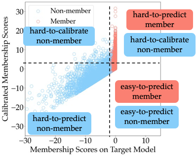
Recent state-of-the-art attacks [3, 37] have explored the difficulty level of each data record and applied parametric calibration to improve the attack performance in the low FPR region. These attacks are similar in design to our proposed method in that each target data record is individually considered when performing attacks. However, these works provided limited discussions on the impact of calibration on different types of data records with varying intrinsic properties. Motivated by this, we categorize member and non-member data records into five categories based on their difficulty levels to predict and calibrate, as shown in Figure 3: hard-to-predict member/non-member, easy-to-predict member/non-member, and hard-to-calibrate non-member.
This figure compares membership scores on the target model and their calibrated counterparts for each data record. The -axis represents the membership score on the target model, while the -axis shows the calibrated membership score. The calibrated membership score is calculated as the difference between the membership score on the target model and that of a reference model. Data records are also labeled with their “hardness” levels in different areas, and members and non-members are marked with different colors. In general, higher scores on the target model’s membership suggest that a data record is a member of the model’s training dataset. This idea has been used in traditional MIAs. However, by correlating these scores with the calibrated membership score, we can gain more insights into the difficulty level of a data record. It is important to note that in our discussions, the difficulty or “hardness” level of a data record is mainly determined by the model in which it is not included as part of the training dataset. Specifically, with regards to member data records, we refer to them as being hard-to-predict when they have low membership scores on the reference model, whereas they are considered easy-to-predict members when their scores are higher. Similarly, for non-members, the difficulty level is determined by their membership scores on the target model. By analyzing this figure, we can get the following insights.
Membership scores on the target model are still useful. MIAs based on loss utilize the gap in cross-entropy loss to differentiate between members and non-members. The basic idea is that members would have smaller loss values (higher membership scores) while non-members would have larger ones. Other score-based attacks also follow a similar approach. However, this type of attack can only accurately identify non-members that are difficult to predict. It cannot identify members with high precision. To solve this problem, difficulty calibration based MIAs use calibrated membership scores instead. The higher the calibrated score, the more likely it is that a data record is member data. These attacks can improve TPR in the low FPR region, as they can better identify hard-to-predict members.
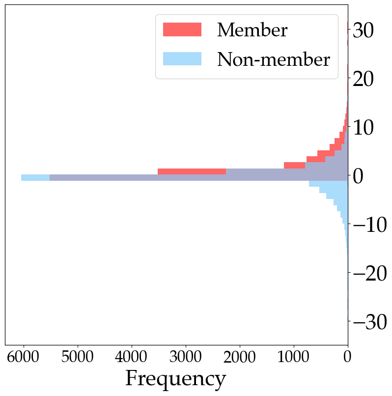
Even though FPR can be reduced by carefully selecting a threshold for the calibrated scores, it is difficult to eliminate all of them. In Figure 3, it can be seen that many non-members overlap with members along the -axis. This can be seen more clearly in Figure 2, which shows the distribution of calibrated membership scores for both members and non-members. In this figure, the calibrated membership scores are on the right -axis and share the same values with that of Figure 3. The -axis shows the number of members and non-members with corresponding calibrated scores. The figure highlights that many members have low calibrated scores, making them easy-to-predict members. These members overlap with non-members near the line where the calibrated score equals 0. Within this region, the easy-to-predict members overlap with both hard-to-predict and easy-to-predict non-members, as both groups have similar outputs on the target and the reference models.
Two things are learned from these observations. Firstly, attackers are likely to encounter easy-to-predict members in real-world attacks, so identifying these samples significantly improves TPR. Secondly, existing difficulty calibration based MIAs may fail to isolate such members from non-members by only considering the calibrated membership scores. But we can see from Figure 3 that moving the vertical dashed line and the horizontal one simultaneously makes it easier to differentiate between members and non-members. This indicates that the membership scores on the target model are still useful in addition to the calibrated membership scores. Based on this observation, we utilize membership scores on the target model in LDC-MIA to exclude the hard-to-predict non-members. This approach not only helps identify hard-to-predict members but also easy-to-predict members, thus improving TPR in all FPR regions.
Neighbor information is also important. In Figure 3, it is evident that some non-members have high calibrated membership scores, indicating that they perform significantly better on the target model than on the reference model. These non-members are not easy-to-predict, as they have low membership scores on the reference model, nor hard-to-predict, as they have high membership scores on the target model. We refer to such non-members as hard-to-calibrate samples, as they cannot be easily distinguished using calibrated membership scores.
According to Long et al., certain data records are at a higher risk of being exploited by attackers if they have fewer neighbors in the sample space represented by the records available to the attacker [24]. This is because such records may impose a unique influence on the target model. In other words, a member data record with fewer neighbors in the training dataset is more likely to be identified by MIAs. Conversely, data records with more neighbors may lead to more incorrect inferences by MIAs. For example, if a non-member data record has many neighbors in the training dataset of the target model, it is more likely to be incorrectly identified as a member compared to another non-member data record that has fewer neighbors. Therefore, it is speculated that the hard-to-calibrate non-members have more neighbors in the target model’s training dataset. In other words, when comparing two data records with high calibrated membership scores, the one with fewer neighbors is more likely to be a member. Hence, LDC-MIA includes neighbor information to differentiate hard-to-predict members and hard-to-calibrate non-members in the upper right region in Figure 3.
The goal is to lower the calibrated membership score for hard-to-calibrate non-members. A similar method proposed by Long et al. is adopted to calculate neighborhood information. First, a data record is fed into the reference model and the output of the last layer before the softmax layer is collected as its neighborhood vector. Then, cosine similarity is computed between this neighborhood vector and those of all the other data records in the auxiliary dataset. Data records with cosine similarity exceeding a certain threshold are considered neighbors. Finally, the neighborhood information of a target data record is computed as follows:
| (7) |
, where is the neighborhood vector of the target data record, is that of the data records in the auxiliary dataset, is the size of the auxiliary dataset, and is the similarity threshold value to determine neighbors. We use in our attack. Through our experiments in Section 4, we verify that setting to 0 works well for most datasets. The intuition behind this is that the value of cosine similarity is greater than 0 when two data records are positively related. We also know that a model’s inference on a target sample is influenced by its neighbor data records if they exist in the training dataset. Therefore, by using a threshold of 0 for the cosine similarity value, we can better distinguish neighbor and non-related data records. Then, we enhance the membership scores proposed by Watson et al. [37] with neighborhood information as follows:
| (8) |
, where is the target model, and is the reference model. This enhancement helps distinguish the hard-to-predict members and hard-to-calibrate non-members by shifting the membership scores differently.
We compare the effect of the enhanced membership score and that of the membership score proposed by Watson et al. in Figure 4.
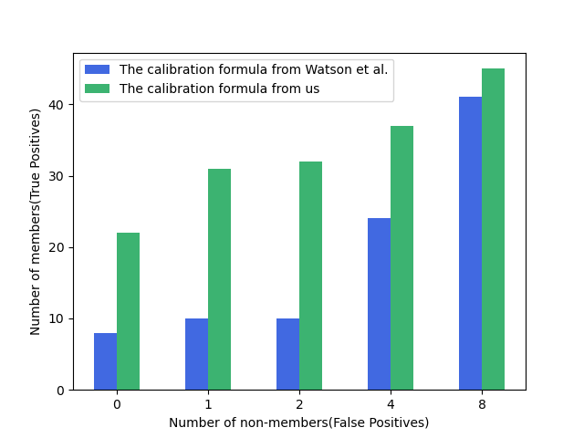
The MIA follows Watson et al.’s approach of using a threshold on calibrated membership scores to determine membership. Based on the figure, it can be observed that the new score can better distinguish members from hard-to-calibrate non-members manifested in improved TPRs at the same low FPRs. It is important to note that we only compared the TPR in the low FPR region because this is the region where MIAs are considered practical. The comparison results suggest that neighborhood information is a valuable and useful component in membership scores.
Different MIA score thresholds are needed for accurately classifying samples with different labels. One of the main objectives of an attacker is to achieve high precision in identifying member data records in the training dataset. To achieve this goal, the attacker strives to differentiate between members and non-members as much as possible. Many existing MIAs rely on a threshold value of the membership scores to distinguish between members and non-members. However, the divergence of membership scores in a target model is influenced not only by the hardness and neighborhood information of a data record but also by its assigned label. This could be attributed to the different distributions of easy and hard data records across various classes. As a result, we believe that determining the most suitable threshold of membership scores for each class can further enhance the accuracy of MIAs. To illustrate this, we present an example of the membership scores of data records in CIFAR-10 belonging to different classes in Figure 5, using the enhanced calibrated membership score calculated by Eq 8. In this example, we use the VGG-16 as both our target and reference models. Both models are trained until they achieve their highest accuracy values on the test dataset.
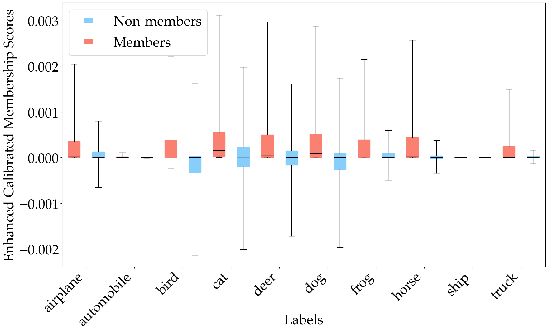
The figure displays the membership score of different data records on the axis, while the axis shows their labels. The scores for member and non-member data records are shown in two different colors. It is evident that the average membership score is higher for members. This means that if an attacker sets a reasonable threshold value, they can identify more members accurately, resulting in high precision. For instance, choosing a threshold of 0.001 can help identify airplanes with high precision without increasing many false positives. However, this may lead to low precision for other classes like deer or cats, which can harm overall precision. Therefore, to maintain overall precision, the attacker should carefully select a threshold value for each class.
3.3 Attack Framework
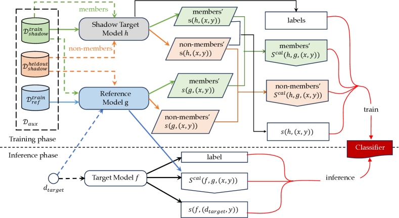
Based on the aforementioned intuitions, we propose to build a classifier that can determine the membership of data records. Our ultimate goal is to utilize the discriminatory abilities of neural network models to establish the optimal threshold for various classes based on the membership scores and neighborhood information. The proposed attack consists of two phases. The first phase is the training phase, in which a shadow target model , a reference model , and an attack classifier are all trained. The second phase is the inference phase, in which we obtain the features of each target data record from the trained reference model and the target model and use the features for classification using the attack classifier. The proposed attack workflow is illustrated in Figure 6.
In the proposed attack, we use an auxiliary dataset that has the same distribution as the data used for training the target model. During the training phase, we first split into three distinct parts. 1. , which is used to train the shadow target model. 2. , which contains non-member data records for the shadow model. 3. , which is used to train the reference model. This way, we can keep a clear separation between the data used for training the different models. The shadow target model should behave similarly to the target model. To achieve this, we train the shadow target model until its validation loss is close to that of the target model. Once all the models are trained, we feed all the data records in and to the shadow target model and the reference model.
We can categorize the membership scores obtained from the shadow target model into four groups: members’ , non-members’ , members’ , and non-members’ . Note that the data records in and are made up of members and non-members of the training dataset of the shadow target model, respectively. This means that the attacking classifier can observe how both members and non-members behave on the shadow target model and the reference model, allowing it to discriminate different behaviors. The reference model is introduced to calibrate the membership scores. Therefore, the membership scores of members on the shadow target model are paired with those on the reference model, and Eq (8) is used to calculate the calibrated membership score . To obtain the neighborhood information of a data record, we exclude the interference of the training data of the reference model by using the data records from and only. These data records consist of in Eq (7). Then, the same process is carried out for non-members to obtain the calibrated membership score.
The membership scores obtained from the target model, as mentioned in Section 3.2, can still be useful in MIAs. We include these scores as one of the features to train the attacking classifier, along with the ground truth label of the data records and the calibrated membership score. With the help of the ground truth membership information, the classifier can learn to predict the membership of a given data record using these features. After training the classifier, we apply it to the actual attack during the inference phase.
During the inference phase, an attacker can only access the target model as a black box. This means that they can only access the label and membership score of a target data record by using the prediction results of the target model. Just like in the training phase, we use and to obtain neighborhood information. Then, we provide to the same reference model that was used during the training phase and calculate the calibrated membership score . Finally, we feed all three values to the classifier to predict the membership of . Our classifier is an MLP model that consists of two hidden layers with ReLU activation functions, followed by a softmax layer.
4 Evaluations
In this section, we conduct a series of experiments to evaluate the performance of the proposed attack on the most widely used datasets and various target model architectures. Additionally, we compare LDC-MIA with several other representative black-box MIA methods[39, 37, 30].
4.1 Experimental Setup
4.1.1 Datasets
In our experiments, we use the following datasets that have been often used for image classifications:
-
•
CIFAR-10[18]. The CIFAR-10 is a benchmark dataset used for image classification tasks. Each image is 32323, and there are 60k images categorized into 10 classes with equal distribution per class.
-
•
CIFAR-100[18]. The CIFAR-100 dataset consists of 100 classes of images, with 32323 sized images and a total of 60k images. Similar to the CIFAR-10 dataset, it is also used for image classifications.
- •
In addition to the image dataset, we also use the following datasets for our experiments:
-
•
Adult[2]. The adult dataset contains information on people’s income, with 2 classes and 14 features for each of the 48842 data records.
-
•
Credit[13]. The Credit dataset is often used for binary classification tasks involving credit scoring. It contains 1000 data records with each consisting of 20 features. There are two classes of data records in the dataset.
In our evaluations, we divide each dataset into five parts: , , , , and . and are utilized as the training and testing dataset for the target model. and , on the other hand, are used to train and test the shadow target model. is the training dataset for the reference model. In our experiments, the datasets are proportionally sized in the ratio of 5:5:3:3:4.
4.1.2 Models
When selecting target models, we prioritize those with better classification accuracy. For the CIFAR-10 and CINIC-10 datasets, we choose VGG-16 as the target model, while for the CIFAR-100 dataset, we use SmallNet, this is to make a fair comparison with the method by Watson et al. [37] where they use SmallNet too. For the remaining datasets, we employ a multi-layer perceptron (MLP) model as the target model, which consists of one hidden layer with ReLU activation function, followed by a softmax layer. The training and testing accuracy of the target models is shown in Table I.
on different datasets.
| Dataset | Target Model | Train Accuracy | Test Accuracy |
|---|---|---|---|
| CIFAR-10 | VGG-16 | 97.62% | 71.71% |
| CIFAR-100 | Smallnet | 94.53% | 31.27% |
| CINIC-10 | VGG-16 | 96.16% | 60.56% |
| Adult | MLP | 92.04% | 83.29% |
| Credit | MLP | 90.62% | 83.23% |
We use the same network architecture as the target model for both the reference model and the shadow target model. We also explore employing different model architectures for the reference model and shadow target model (results are detailed in Section 5). When training the shadow target model, its validation loss does not need to be similar to the target model (this non-requirement is practically useful since our method doesn’t assume the attacker needs to know the target model training validation loss). The reference model is trained until it reaches the maximum validation accuracy. Our proposed MIA classifier is of multi-layer-perceptron architecture, that consists of two hidden layers with ReLU activation functions, followed by a softmax layer. We utilize stochastic gradient descent (SGD) with a learning rate of 0.1, Nesterov momentum of 0.9, and a cosine learning rate schedule for the training. The duration of training for each model varies between 20 to 200 epochs, depending on the complexity of the models and the size of the datasets.
4.1.3 Metrics
In our experiments, we use the following metrics to evaluate the results of the MIAs:
-
•
Full Log-scale ROC. In evaluating the accuracy of MIAs, precision is an important metric. Carlini et al. [3] suggest that the TPR should be emphasized in low FPR regions, as higher TPR in these regions indicates higher precision of the MIA method. A full log-scale receiver operating characteristic (ROC) curve can be used for a clearer comparison of TPR among different MIAs in low FPR regions.
-
•
TPR at Low FPR. We also analyze the TPR of various MIA methods at a few low FPR points, including 1%, 0.1%, and 0.01%. These values enable numerical comparisons between different MIA methods.
-
•
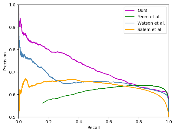
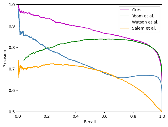
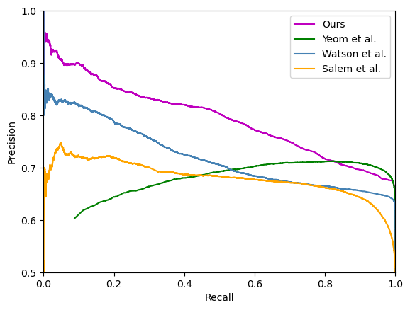
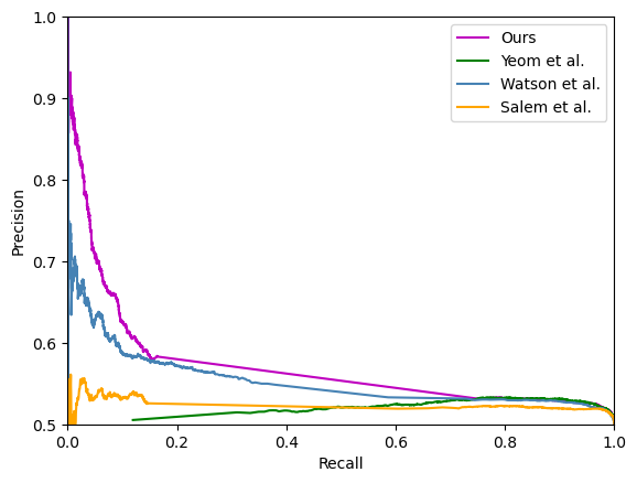
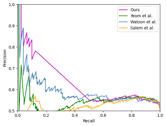
Precision-Recall (PR) Curve In real-world scenarios, attackers are more likely to encounter members that are easy to predict into the model than those that are hard to predict, as indicated in Figure 2. Therefore, most MIAs can achieve high recall rates by identifying such members. However, recall only measures the effectiveness of the model in capturing most of the positive instances, it does not reflect how accurately the model predicts positives. Therefore, it is also important to measure precision values at relatively high recall rates. We can do this by looking at the precision values when the recall value ranges between 0.2 and 0.7. This metric helps us measure how effectively the model balances between precision and recall.
-
•
Balanced accuracy and AUC. As with previous MIA methods [26, 32, 37], we measure the overall performance of LDC-MIA using Balanced accuracy and AUC. When working with imbalanced datasets, accuracy alone can be misleading. Hence, balanced accuracy is an important metric often used to evaluate the performance of a classification model by considering the arithmetic mean of TPR and TNR. On the other hand, AUC quantifies the overall performance of the model by measuring the area under the ROC curve.
4.1.4 Baselines
In our evaluations, we compared LDC-MIA with three other MIA methods. Salem et al. [30] used the posteriors of target data records obtained from the target model and trained a shadow model to mimic the target model’s behaviors. They proposed three different adversary models, and we compared LDC-MIA with Adversary 1, which had the best performance. Yeom et al. [39] performed the attack without any auxiliary model by using the loss values of the target data records on the target model. Watson et al. [37] used a reference model for difficulty calibration when performing MIA. To ensure a fair comparison, we used the same auxiliary dataset and two auxiliary models — one shadow model and one reference model — in our proposed attack. For other MIA methods, we use two reference or shadow models if they employ any.
4.2 Main Results
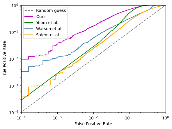
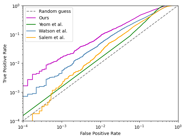
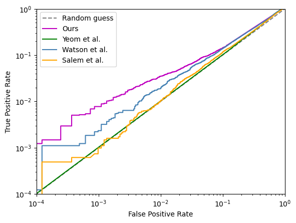
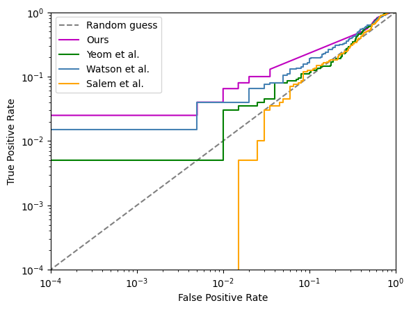
In this section, we present the results of our proposed attack method and compare it with other MIA methods. All the attacks are carried out in the black-box scenario, and we demonstrate and analyze the results using various metrics as mentioned in Section 4.1. Furthermore, we compare the attack performance and cost of LDC-MIA with LiRA [3], the current state-of-the-art MIA method.
| Attack method | CIFAR-10 | CIFAR-100 | CINIC-10 | Adult | Credit | ||||||||||
|---|---|---|---|---|---|---|---|---|---|---|---|---|---|---|---|
| 0.01% | 0.1% | 1% | 0.01% | 0.1% | 1% | 0.01% | 0.1% | 1% | 0.01% | 0.1% | 1% | 0.01% | 0.1% | 1% | |
| Salem et al. [30] | 0.00% | 0.1% | 1.6% | 0.04% | 0.3% | 2.3% | 0.00% | 0.2% | 2.3% | 0.00% | 0.1% | 1.0% | 0.00% | 0.0% | 0.0% |
| Yeom et al. [39] | 0.01% | 0.0% | 0.0% | 0.04% | 0.2% | 1.0% | 0.00% | 0.0% | 0.0% | 0.00% | 0.0% | 0.0% | 0.50% | 0.5% | 3.0% |
| Watson et al. [37] | 0.05% | 0.5% | 3.5% | 0.32% | 1.1% | 5.9% | 0.07% | 0.4% | 4.0% | 0.01% | 0.2% | 2.0% | 1.50% | 1.5% | 4.0% |
| Ours | 0.27% | 1.8% | 6.4% | 0.95% | 3.8% | 16.4% | 0.16% | 1.6% | 8.7% | 0.15% | 0.8% | 3.5% | 2.50% | 2.5% | 6.5% |
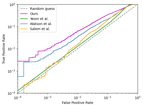
4.2.1 TPR at low FPR regions
In this experiment, we compare the TPR-FPR tradeoff of our method LDC-MIA and three other MIA methods across five datasets. The ROC curves for all methods over five datasets are depicted in Figure 7. The figure shows that LDC-MIA achieves higher TPR at almost all FPRs than other MIA methods across all datasets. Further, we compare the TPR values in the low FPR region (i.e., between and ) with results obtained from an average of 5 runs in Table II, The results show that LDC-MIA achieves better TPRs in the low FPR region. On CIFAR-100 and CINIC-10 datasets, LDC-MIA outperforms the state-of-the-art difficulty calibration-based MIA method proposed by Watson et al., having 4x higher TPRs in low FPRs.
| Attack method | CIFAR-10 | CIFAR-100 | CINIC-10 | Adult | Credit | |||||
|---|---|---|---|---|---|---|---|---|---|---|
| Balanced acc | AUC | Balanced acc | AUC | Balanced acc | AUC | Balanced acc | AUC | Balanced acc | AUC | |
| Salem et al. [30] | 66.30% | 0.703 | 66.54% | 0.697 | 70.14% | 0.745 | 53.59% | 0.539 | 60.50% | 0.563 |
| Yeom et al. [39] | 69.65% | 0.694 | 84.82% | 0.889 | 77.12% | 0.780 | 55.33% | 0.546 | 60.25% | 0.581 |
| Watson et al. [37] | 66.88% | 0.711 | 73.78% | 0.772 | 71.80% | 0.768 | 54.90% | 0.566 | 59.25% | 0.607 |
| Ours | 67.93% | 0.754 | 85.12% | 0.918 | 75.71% | 0.832 | 55.36% | 0.577 | 58.75% | 0.608 |
4.2.2 Precision-Recall curve
We compare MIA methods’ effectiveness by examining the precision and recall tradeoffs made by our method and three others. The Precision-recall curves of all MIA methods across five datasets are depicted in Figure 8. Our method LDC-MIA reaches the highest precision values over most of the recall value range compared to other MIA methods, across all datasets. For the CIFAR-100 dataset, LDC-MIA achieves a recall rate of for members with a precision of . For the CIFAR-10 dataset, the recall is with a precision of . For the CINIC-10 dataset, LDC-MIA identifies of the members with a precision of .
4.2.3 Balanced accuracy and AUC
The balanced accuracy is the arithmetic mean of sensitivity and specificity, the higher the better. AUC value indicates the overall discriminatory power of the model over all possible TPR-FPR tradeoffs, the higher the better. Table III shows the balanced Accuracy and AUC of all the MIA methods averaged out of 5 runs. The highest metric values and the metric values of LDC-MIA have been highlighted. LDC-MIA achieves the highest AUC values across all the datasets. Regarding balanced accuracy values, LDC-MIA has close if not better results compared to the best-performing MIAs.
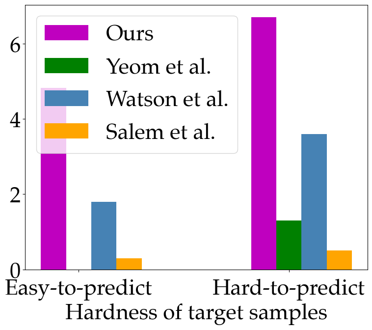
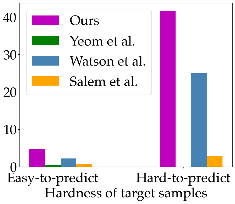
4.2.4 Improvement on TPR at various hardness levels
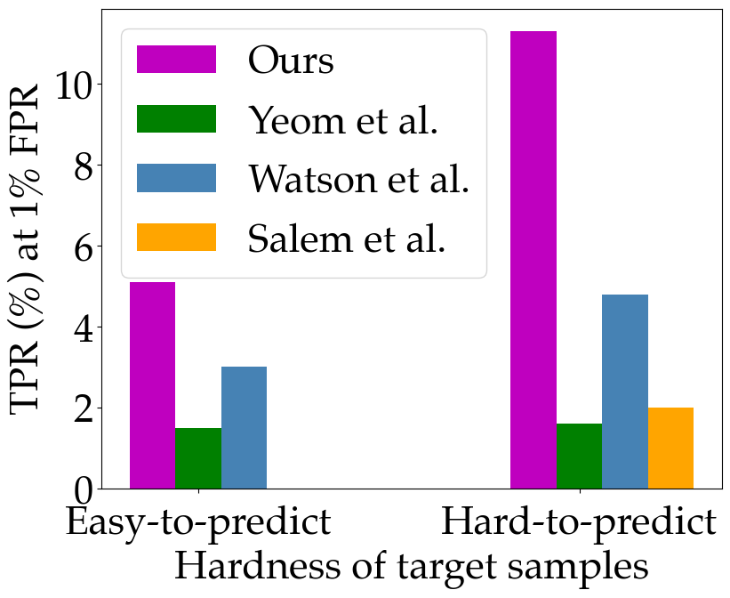
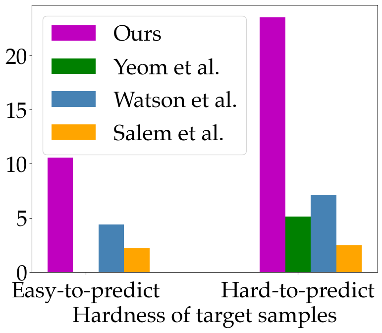
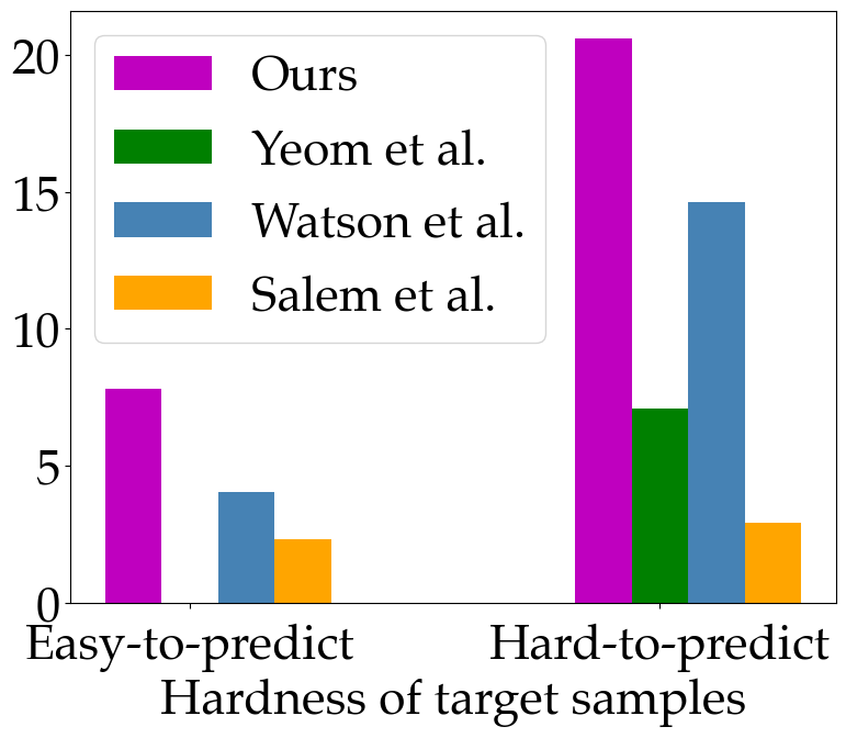
Data records of different hardness levels may have different vulnerabilities to membership inference attacks. Therefore, we categorize data from different datasets into two groups based on their membership scores on the reference model: the hard-to-predict and easy-to-predict samples. Note that neither the member nor the non-member data records are in the training dataset of the reference model. To determine which group each data record belongs to, we use a threshold value. For non-binary class datasets, if a data record’s membership score falls in the range of , it is classified as an easy-to-predict sample; otherwise, it is classified as a hard-to-predict sample. For binary class datasets such as Adult and Credit, the ranges for easy-to-predict and hard-to-predict samples are and , respectively. The TPR values of different MIAs are shown in Figure 9. Note that all the figures share the same label on axis: TPR at FPR. We can see that LDC-MIA significantly improves the TPR for both easy-to-predict and hard-to-predict samples across all datasets. However, for threshold-based MIA, such as the one proposed by Yeom et al., it could easily misclassify all member samples. In this experiment, the identification of both hard-to-predict and easy-to-predict members has been improved by the combination of calibrated membership score and membership score on the target model in the classifier.
4.3 Effect of data augmentation
Data augmentation is a technique that can be used to increase the size of a dataset by applying different transformations to existing training data. This technique is often used to improve the generalization and robustness of models. By exposing the model to a wider range of data variations, it can learn to handle different input scenarios, resulting in better performance. In this experiment, we applied data augmentation during the training of the target model and the shadow models (if any), and then evaluated its effect on the MIAs by measuring its AUC and TPR at FPR values. Note that we used horizontal flipping for the shadow (target) models training, and random cropping and rotation for the target model training. This is important because attackers may not have access to the data augmentation techniques used in the target model in real-life situations. The results of the experiment are shown in Table IV and Table V, where we only present the results for the CIFAR-10 and CIFAR-100 datasets due to space limitations.
| Attack method | CIFAR-10 | CIFAR-100 | ||
|---|---|---|---|---|
| w/o aug | w aug | w/o aug | w aug | |
| Salem et al. [30] | 0.703 | 0.612 | 0.697 | 0.625 |
| Yeom et al. [39] | 0.694 | 0.601 | 0.889 | 0.802 |
| Watson et al. [37] | 0.711 | 0.667 | 0.772 | 0.709 |
| Ours | 0.754 | 0.719 | 0.918 | 0.869 |
on TPR at FPR
| Attack method | CIFAR-10 | CIFAR-100 | ||
|---|---|---|---|---|
| w/o aug | w aug | w/o aug | w aug | |
| Salem et al. [30] | 1.6% | 0.5% | 2.3% | 0.6% |
| Yeom et al. [39] | 0.0% | 0.0% | 1.0% | 0.0% |
| Watson et al. [37] | 3.5% | 1.1% | 5.9% | 2.7% |
| Ours | 6.4% | 3.6% | 16.4% | 12.4% |
From the results, it can be observed that both AUC and TPR decrease when data augmentation is applied. This is because data augmentation reduces overfitting, thereby reducing the effect of MIAs [39]. However, LDC-MIA has not been affected as much as the other MIA methods. This suggests that our proposed attack is robust against data augmentation in the target model training.
4.4 Comparison with LiRA
The likelihood ratio attack (LiRA) [3] is a state-of-the-art MIA that can achieve a high TPR at low FPR regions. To determine membership, LiRA calculates the likelihood ratio, which represents the ratio of the likelihood of a data point being in the target model’s training dataset to the likelihood of it being from a different, unknown dataset. The likelihood ratio is computed based on the output probabilities of shadow models. The membership is determined based on the likelihood ratio. However, online LiRA attack is computationally intensive, because, for every new (batch) of target instance(s), LiRA needs to train multiple new shadow and reference models, with and without these instances. Note that LDC-MIA only utilizes two auxiliary models: the shadow target model and the reference model in the experiments. The same neural network classifier in LDC-MIA, trained with data provided by the shadow target model and reference model, can be re-used and attack new target instances without any need for additional model training.
| Attack method | ResNet-18 | ResNet-34 | ||
|---|---|---|---|---|
| 0.1% | 1% | 0.1% | 1% | |
| LiRA(N=2) | 1.5% | 4.6% | 1.2% | 4.7% |
| LiRA(N=4) | 1.5% | 5.6% | 1.7% | 5.3% |
| LiRA(N=6) | 1.7% | 5.8% | 2.0% | 5.9% |
| LiRA(N=8) | 1.9% | 5.7% | 2.0% | 6.0% |
| Ours | 2.6% | 10.7% | 2.1% | 8.8% |
In the comparison experiment, we select ResNet-18 and ResNet-34 trained on CIFAR-10 as the target models. The TPR at low FPR regions are shown in Table VI, both LDC-MIA and LiRA.
4.5 Cost-Performance Trade-off
In real attack scenarios, the cost associated with an attack is also a crucial factor. Thus, in this section, we compare the trade-off between cost and performance among the MIAs that we have evaluated. We use the TPR at FPR as the metric to evaluate the performance of MIAs. On the other hand, We use the number of auxiliary models required to launch the attack as the proxy metrics for the cost of the attack, this metric approximates both the computational cost and the data cost.
Table VII includes the TPR results obtained from attacking the CIFAR-10 dataset with ResNet-18 as the target model, and the number of shadow and reference models required for each attack method. It is important to note that the LiRA method needs to train 8 (or 256, depending on the setting) shadow models for every target instance. Thus, the total cost is not a constant, but rather linear to the number of target instances. We also note that our method LDC-MIA needs to train a neural network-based MIA classifier in addition to one shadow model and one reference model. This model uses a shallow MLP architecture. It poses a similar or less cost than training a shadow model in all of the datasets we experiment, and significantly less in the case where the shadow model is a DNN-based image model.
| Attack | Shadow | Reference | TPR |
| Method | Models | Models | at FPR |
| LiRA[3](N=8) | 8 | - | 1.9% |
| LiRA[3](N=256) | 256 | - | 8.1% |
| Watson et al. [37](N=1) | - | 1 | 0.9% |
| Watson et al. [37](N=10) | - | 10 | 1.4% |
| Salem et al. [30] | 1 | - | 0.2% |
| Yoem et al. [39] | - | - | 0.0% |
| Ours | 1 | 1 | 2.6% |
The table shows that LiRA can achieve the highest TPR if 256 shadow models are trained for each target sample. However, our proposed attack method reduces the cost of attacking significantly. Meanwhile, it still manages to achieve a higher TPR than all other existing MIAs. The results indicate that LDC-MIA strikes an outstanding balance between performance and cost.
5 Ablation Study
5.1 Differential Privacy
In order to evaluate the robustness of our proposed attack, we utilize the concept of differential privacy during the training of the target model. This technique adds noise or randomization to the data, which helps protect individual privacy in datasets. It can be useful in limiting the effectiveness of many existing MIAs [37, 3, 39]. We use DP-SGD [1], one of the state-of-the-art mechanisms, for training the target model in our experiments. DP-SGD adds carefully calibrated noise to the gradients computed during each iteration. The amount of noise added depends on the sensitivity of the gradients and the desired privacy budget . While a smaller provides stronger privacy guarantees, it can also result in noisier updates. The other two important parameters in DP-SGD are the clipping bound and the noise multiplier .
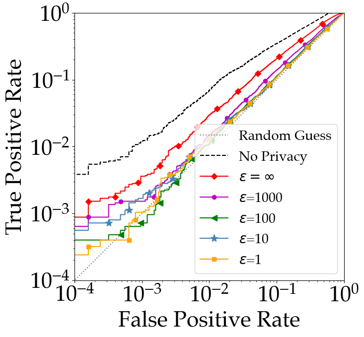
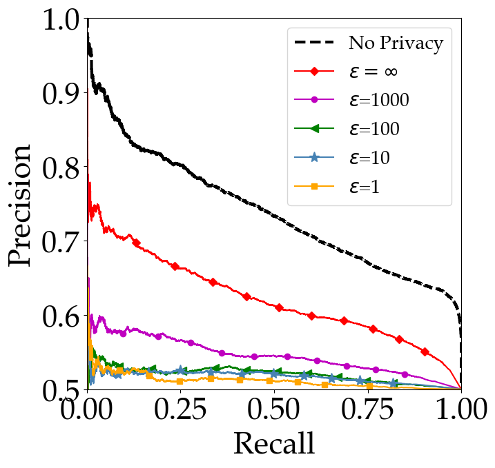
The clipping bound is a threshold value applied to the gradients computed during training. This operation limits the influence of any single data point on the model’s parameters. The noise multiplier is a parameter that determines the amount of noise added to the gradients during each iteration of the training. In practice, to achieve a specific privacy budget , one can adjust the noise multiplier and the total number of iterations. In our experiments, we set to and vary from to to adjust . We evaluate the performance of the proposed attack at different values (, 1000, 100, 10, and 1). The PR curve and the ROC curve are shown in Figure 10, and the AUC and TPR are shown in Table VIII.
| Model acc | AUC | TPR at 0.1%FPR | ||
|---|---|---|---|---|
| 0 | 64.51% | 0.646 | 0.3% | |
| 0.2 | 1000 | 59.35% | 0.560 | 0.2% |
| 0.3 | 100 | 52.56% | 0.529 | 0.1% |
| 0.6 | 10 | 43.65% | 0.524 | 0.2% |
| 1 | 1 | 28.91% | 0.513 | 0.1% |
From the figure and the table, it is evident that as the desired privacy budget increases, both AUC and TPR decrease. However, in practice, there is a trade-off between privacy () and utility (the accuracy of the trained model). When higher privacy is required, adding more noise can significantly affect the model’s utility. This is evident from the model accuracy column in Table VIII. In practice, to preserve model accuracy, reasonable values of , such as 100 or 1000, are more likely to be used. It is observed that AUC and TPR are not significantly reduced in these cases. Moreover, even with small values, the proposed attack can still achieve high precision values () at low recall, as seen from Figure 10(b).
5.2 Overfitting Level of the Target Model
Previous studies [30, 32] have demonstrated that the performance of MIAs is closely related to the overfitting level of the target model. Overfitting happens when the model learns the training data too well, including noise and specific patterns that are unique to the training set. There are several factors that can affect the overfitting level of a model, such as dataset size and quality, training duration, model complexity, and regularization. To vary the overfitting level of the target model in our experiments, we adjust the training dataset size between 6500 and 12500. Typically, increasing the size of the training dataset helps reduce overfitting, while decreasing it has the opposite effect. A larger and more diverse dataset allows the model to learn a wider range of patterns and variations present in the data. Meanwhile, we keep the size of the training dataset of the reference model and that of the shadow target model fixed. We then measure the impact of the overfitting level by evaluating AUC and TPR of the proposed attack. The results are shown in Table IX.
| Training dataset size | Train Test | LDC-MIA | |
|---|---|---|---|
| Acc Gap | AUC | TPR at FPR | |
| 6500 | 37.91 | 0.787 | 8.1% |
| 8000 | 36.28 | 0.783 | 7.6% |
| 9500 | 34.08 | 0.770 | 7.3% |
| 11000 | 29.96 | 0.761 | 6.1% |
| 12500 | 26.91 | 0.754 | 5.7% |
In Table IX, we can observe that the overfitting level of the target model increases as the size of its training dataset decreases. This can be seen from the gap between the training accuracy and test accuracy of the target model. The larger the gap between these two, the more the model is overfitting. Furthermore, we can also see that the AUC and TPR at FPR improve slightly as the overfitting level of the target model increases.
5.3 Training Dataset Sizes for the Shadow Target and the Reference Models
An important factor in our proposed attack is the size of the datasets used to train the shadow target and reference models. As discussed in Section 5.2, the training dataset sizes affect the performance of the trained shadow target and reference models, leading to performance variance in the proposed attack. To evaluate this factor, we divide an auxiliary dataset consisting of 25k data records into two parts: for training the shadow target model and for training the reference model. We set up two configurations to vary the sizes of and . In the first configuration, we fix to be of and vary the size of . In the second configuration, we do the opposite by fixing to be of and vary the size of . We then evaluate the TPR at FPR of LDC-MIA on the VGG-16 target model trained with the CIFAR-10 dataset. The results are shown in Figure 11. Note that the two subfigures have the same label on axis.
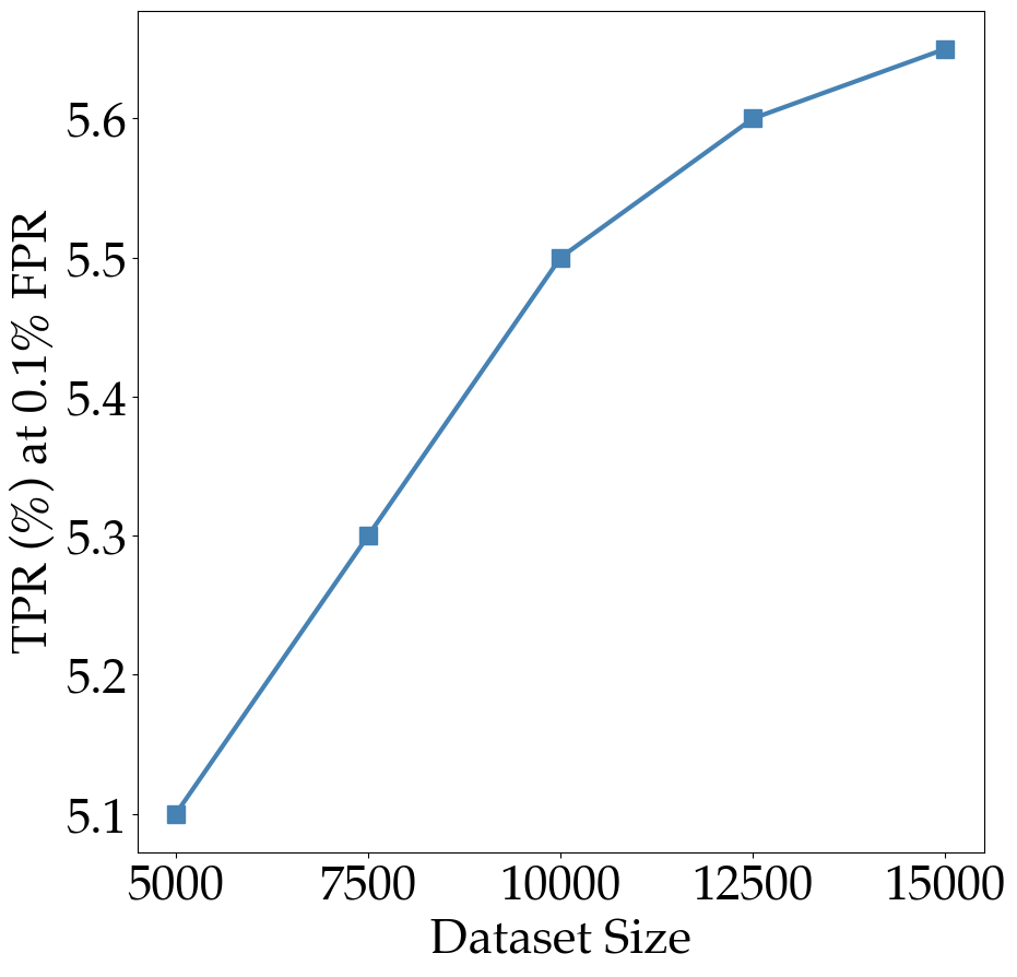
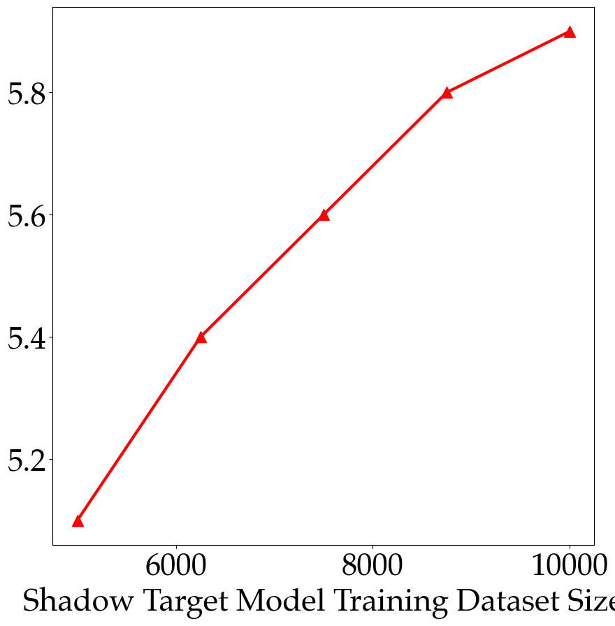
The figure shows that increasing the size of the datasets, and , improves the TPR of LDC-MIA. When the size of is increased, the MIA classifier is exposed to a wider range of membership scores and more calibrated membership scores from the target samples, which in turn improves the generalization of the shadow target model. On the other hand, when the size of is increased, the attacker can obtain more accurate calibrated membership scores by improving the discriminative power of the reference model. The figures also show that the impact of the size of is similar to that of the size of .
5.4 Model Architectures
Attackers in real-world scenarios may not have knowledge about the architecture of the target model. To analyze the impact of having different network architectures in the shadow target model on the performance of our proposed attack, we randomly select two models from VGG-16, ResNet-18, ResNet-34, and Smallnet as the target and shadow target models while keeping the reference model’s architecture the same as the shadow target model. We evaluate the performance of LDC-MIA using AUC and TPR at FPR as metrics, and we use the CIFAR-10 dataset in this experiment. The results are shown in Figure 12.
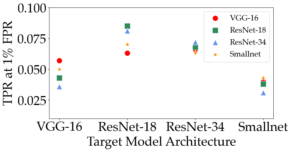
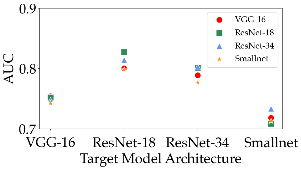
Different shapes are used in the figure to represent different shadow target model architectures. It can be observed from the figure that, in general, the architecture of the shadow target model has little impact on the attack performance. For TPR values, we can see that LDC-MIA performs the best when the shadow target model shares the same architecture as the target model from Figure 12(a). However, for AUC, LDC-MIA can achieve the highest value when the two model architectures are different in some cases, as demonstrated in Figure 12(b). For instance, when the target model is VGG-16, the best-performing shadow target model is ResNet-18. It is worth noting that even in the worst cases, LDC-MIA still achieves better TPR than the other MIA methods we have compared with, as shown in Table II. These results are encouraging as they indicate that the attackers are not limited to specific model architectures with our proposed attack.
5.5 Model Learning Optimizers
There are various choices of optimizers for the training of machine learning models, such as SGD, SGDM, and ADAM. Some optimizers provide better regularization, leading to better generalization and reduced overfitting. For instance, ADAM, a commonly used optimizer, is considered helpful in mitigating memorization. In this experiment, we investigate (1) What impact does the optimizer’s choice have on the attack performance? and (2) Does knowing which optimizer is used in the target model improve attack performance? We use VGG-16 model trained on CIFAR-10 dataset for this experiment.
Figure 13 presents the TPR values at low FPR values, with the target model’s optimizer shown on the -axis, and different markers indicating the performance of various optimizers used in the shadow target model.
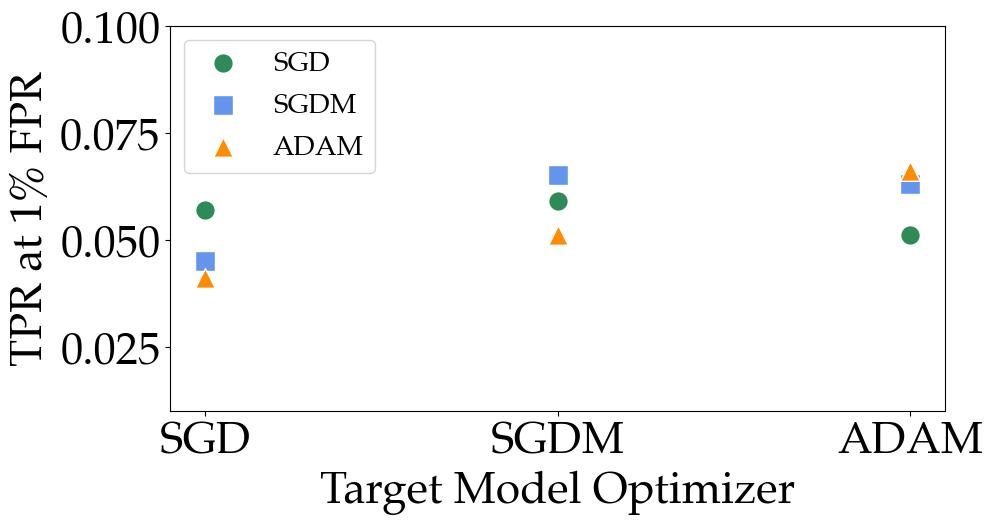
Figure 13 indicates that there is no significant effect on attack performance by varying optimizers for training the target model. The figure also shows that for every optimizer we test, the attacker can achieve the highest TPR by applying the same optimizer in the shadow target model as in the target model. Applying SGDM in the shadow target model always tends to achieve better attack performance if the exact optimizer in the target model is unknown to the attacker.
5.6 Different Features
To evaluate the impact of the features introduced into the classifier, we remove each of them from the model and compare the performance of the proposed attack. The proposed classifier has three features — membership scores on the target model, calibrated membership scores, and labels. We compare the contribution of each feature to the attack by analyzing the full log-scale ROC curves. The target model in this experiment is VGG-16 trained on CIFAR-10. The results are shown in Figure 14. From the figure, we can see that removing any of the features results in a degraded performance of the attack, and each of them contributes differently to the attack.
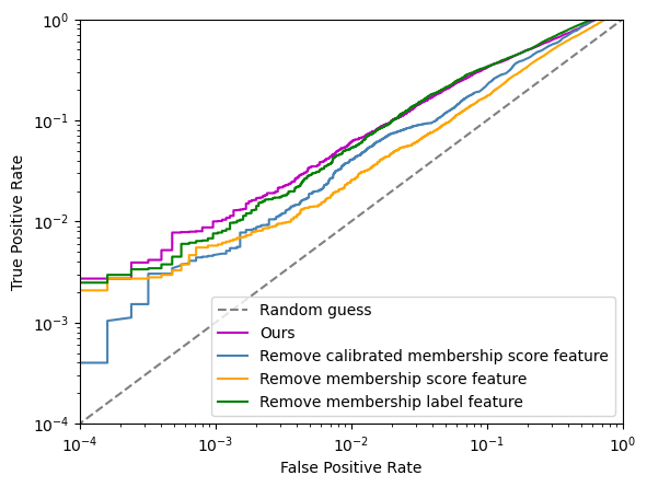
Firstly, removing the label feature leads to a reduction in TPR at low FPR. This indicates that the label feature helps reduce false positives, leading to improved TPR, especially at low FPR. Secondly, removing the membership score reduces TPR in all FPR regions. This verifies what we discussed in Section 3.2 — that including the membership scores not only helps identify hard-to-predict members but also easy-to-predict members, thus improving TPR in all FPR regions. Finally, the performance of the proposed attack significantly degrades by excluding the calibrated membership scores. This is because the calibrated membership scores help separate the hard-to-predict members from the easy-to-predict non-members, which is a significant portion of the non-members, easily. Overall, all three features contribute significantly to the success of our proposed attack.
6 Related Works
6.1 Membership Inference Attacks
Although membership Inference Attacks (MIA) can serve as an audit mechanism to verify the privacy of machine learning models [33, 12, 30, 22], they have become a major concern for privacy if used by miscreants, to leak sensitive data in the training dataset of the models.
In traditional MIAs, such as the work by Shokri et al. [32], attackers utilize the auxiliary dataset to train several shadow models to mimic the behavior of the target model. By analyzing the output generated by these shadow models, attackers can train a binary classifier that captures the difference in confidence scores for members and non-members of the shadow models. This binary classifier is then used to infer whether a target sample is a member or not based on its confidence score obtained from the target model. Salem et al. [30] proposed a similar attack using shadow model and classifiers but only using a single shadow model, which significantly reduces the cost associated with executing MIAs. These early techniques set the foundation for subsequent research by demonstrating the feasibility of MIAs.
Yeom et al. found that the success of MIAs is positively correlated with model overfitting, which they leverage to identify members by thresholding its membership score. If the score exceeds a pre-defined threshold, the sample is deemed a member. There are similar approaches for MIA by metrics thresholding [29, 33, 5]. Most of these works, set the threshold through simple statistics, while our method LDC-MIA uses a machine learning algorithm to identify more accurate thresholds that are learned by the algorithm from data.
More advanced MIAs use statistical methods, such as likelihood ratios and hypothesis testing, to distinguish subtle patterns in model behaviors trained with certain samples [37, 3, 24]. Some of these methods use auxiliary models to measure the differences in model behavior with or without a sample Difficulty calibration is introduced to better characterize the differences for different groups of instances based on their difficulty for MIA. Watson et al. [37] introduced a calibrated membership score that improves the attack performance by taking into account the hardness of individual samples. Carlini et al. [3] extended this concept by proposing Likelihood Ratio Attacks (LiRA) that sample dozens to hundreds of shadow models for each instance to characterize the differences between models trained with that instance and those without. In our work, we introduce several features to characterize the instances and leverage them for better difficulty calibration. To the best of our knowledge, LiRA achieves the highest TPRs at low FPRs. However, the online LiRA attack method requires training hundreds of auxiliary models for each target sample to achieve optimal attack performance. We consider it to be excessively expensive for real-world attacks. Our method LDC-MIA is orders of magnitude less expensive while achieving close performance in some of the datasets.
6.2 Defense Against MIA
Some defense methods mitigate MIAs by reducing the excessive memorization of training data by the target model. For example, training models with DP-SGD learning algorithm [1], which incorporates differential privacy related metrics in the learning objective. In our ablation study, we show that the use of DP-SGD in the target model indeed impacts the performance of our MIA method. The downsides of differential-privacy methods tend to lead to reduced target model accuracy. Additionally, regularization techniques such as dropout [34] and weight decay [19] defend against MIAs by lowering the model’s overfitting. Recently, studies such as DMP [31], SELENA [35], and PATE [28] use knowledge distillation to defend MIA and demonstrate some success, while study in [16] shows that distillation alone provides only limited privacy across a number of domains.
7 Conclusion
In this paper, we delve into the difficulty calibration based MIAs and propose a novel learning-based attack, called LDC-MIA. This attack improves the performance of MIA, particularly the TPRs at low FPRs, by using features that characterize the hardness levels of data records. To achieve this, we leverage target samples’ labels, neighborhood information, calibrated membership score, and membership score on the target model. Our experiments show that LDC-MIA can achieve state-of-the-art performance in terms of TPRs at low FPRs, AUC, and precision at high recall rates while keeping the attack cost low.
References
- [1] Martin Abadi, Andy Chu, Ian Goodfellow, H Brendan McMahan, Ilya Mironov, Kunal Talwar, and Li Zhang. Deep learning with differential privacy. In Proceedings of the 2016 ACM SIGSAC conference on computer and communications security, pages 308–318, 2016.
- [2] Barry Becker and Ronny Kohavi. Adult. UCI Machine Learning Repository, 1996. DOI: https://doi.org/10.24432/C5XW20.
- [3] Nicholas Carlini, Steve Chien, Milad Nasr, Shuang Song, Andreas Terzis, and Florian Tramer. Membership inference attacks from first principles. In 2022 IEEE Symposium on Security and Privacy (SP), pages 1897–1914. IEEE, 2022.
- [4] Dingfan Chen, Ning Yu, Yang Zhang, and Mario Fritz. Gan-leaks: A taxonomy of membership inference attacks against generative models. In Proceedings of the 2020 ACM SIGSAC conference on computer and communications security, pages 343–362, 2020.
- [5] Christopher A Choquette-Choo, Florian Tramer, Nicholas Carlini, and Nicolas Papernot. Label-only membership inference attacks. In International conference on machine learning, pages 1964–1974. PMLR, 2021.
- [6] Ekin D Cubuk, Barret Zoph, Dandelion Mane, Vijay Vasudevan, and Quoc V Le. Autoaugment: Learning augmentation policies from data. arXiv preprint arXiv:1805.09501, 2018.
- [7] Luke N Darlow, Elliot J Crowley, Antreas Antoniou, and Amos J Storkey. Cinic-10 is not imagenet or cifar-10. arXiv preprint arXiv:1810.03505, 2018.
- [8] Jia Deng, Wei Dong, Richard Socher, Li-Jia Li, Kai Li, and Li Fei-Fei. Imagenet: A large-scale hierarchical image database. In 2009 IEEE conference on computer vision and pattern recognition, pages 248–255. Ieee, 2009.
- [9] Kang Fu, Dawei Cheng, Yi Tu, and Liqing Zhang. Credit card fraud detection using convolutional neural networks. In Neural Information Processing: 23rd International Conference, ICONIP 2016, Kyoto, Japan, October 16–21, 2016, Proceedings, Part III 23, pages 483–490. Springer, 2016.
- [10] Mohammad Havaei, Axel Davy, David Warde-Farley, Antoine Biard, Aaron Courville, Yoshua Bengio, Chris Pal, Pierre-Marc Jodoin, and Hugo Larochelle. Brain tumor segmentation with deep neural networks. Medical image analysis, 35:18–31, 2017.
- [11] Jamie Hayes, Luca Melis, George Danezis, and Emiliano De Cristofaro. Logan: Membership inference attacks against generative models. arXiv preprint arXiv:1705.07663, 2017.
- [12] Xinlei He, Zheng Li, Weilin Xu, Cory Cornelius, and Yang Zhang. Membership-doctor: Comprehensive assessment of membership inference against machine learning models. arXiv preprint arXiv:2208.10445, 2022.
- [13] Hans Hofmann. Statlog (German Credit Data). UCI Machine Learning Repository, 1994. DOI: https://doi.org/10.24432/C5NC77.
- [14] Bo Hui, Yuchen Yang, Haolin Yuan, Philippe Burlina, Neil Zhenqiang Gong, and Yinzhi Cao. Practical blind membership inference attack via differential comparisons. arXiv preprint arXiv:2101.01341, 2021.
- [15] Robert A Jacobs. Increased rates of convergence through learning rate adaptation. Neural networks, 1(4):295–307, 1988.
- [16] Matthew Jagielski, Milad Nasr, Christopher Choquette-Choo, Katherine Lee, and Nicholas Carlini. Students parrot their teachers: Membership inference on model distillation. arXiv preprint arXiv:2303.03446, 2023.
- [17] Bargav Jayaraman, Lingxiao Wang, Katherine Knipmeyer, Quanquan Gu, and David Evans. Revisiting membership inference under realistic assumptions. arXiv preprint arXiv:2005.10881, 2020.
- [18] Alex Krizhevsky, Geoffrey Hinton, et al. Learning multiple layers of features from tiny images. 2009.
- [19] Anders Krogh and John Hertz. A simple weight decay can improve generalization. Advances in neural information processing systems, 4, 1991.
- [20] Yann LeCun, Léon Bottou, Yoshua Bengio, and Patrick Haffner. Gradient-based learning applied to document recognition. Proceedings of the IEEE, 86(11):2278–2324, 1998.
- [21] Klas Leino and Matt Fredrikson. Stolen memories: Leveraging model memorization for calibrated White-Box membership inference. In 29th USENIX security symposium (USENIX Security 20), pages 1605–1622, 2020.
- [22] Zheng Li, Yiyong Liu, Xinlei He, Ning Yu, Michael Backes, and Yang Zhang. Auditing membership leakages of multi-exit networks. In Proceedings of the 2022 ACM SIGSAC Conference on Computer and Communications Security, pages 1917–1931, 2022.
- [23] Yunhui Long, Vincent Bindschaedler, Lei Wang, Diyue Bu, Xiaofeng Wang, Haixu Tang, Carl A Gunter, and Kai Chen. Understanding membership inferences on well-generalized learning models. arXiv preprint arXiv:1802.04889, 2018.
- [24] Yunhui Long, Lei Wang, Diyue Bu, Vincent Bindschaedler, Xiaofeng Wang, Haixu Tang, Carl A Gunter, and Kai Chen. A pragmatic approach to membership inferences on machine learning models. In 2020 IEEE European Symposium on Security and Privacy (EuroS&P), pages 521–534. IEEE, 2020.
- [25] Ilya Loshchilov and Frank Hutter. Sgdr: Stochastic gradient descent with warm restarts. arXiv preprint arXiv:1608.03983, 2016.
- [26] Luca Melis, Congzheng Song, Emiliano De Cristofaro, and Vitaly Shmatikov. Exploiting unintended feature leakage in collaborative learning. In 2019 IEEE symposium on security and privacy (SP), pages 691–706. IEEE, 2019.
- [27] Milad Nasr, Reza Shokri, and Amir Houmansadr. Comprehensive privacy analysis of deep learning: Passive and active white-box inference attacks against centralized and federated learning. In 2019 IEEE symposium on security and privacy (SP), pages 739–753. IEEE, 2019.
- [28] Nicolas Papernot, Martín Abadi, Ulfar Erlingsson, Ian Goodfellow, and Kunal Talwar. Semi-supervised knowledge transfer for deep learning from private training data. arXiv preprint arXiv:1610.05755, 2016.
- [29] Alexandre Sablayrolles, Matthijs Douze, Cordelia Schmid, Yann Ollivier, and Hervé Jégou. White-box vs black-box: Bayes optimal strategies for membership inference. In International Conference on Machine Learning, pages 5558–5567. PMLR, 2019.
- [30] Ahmed Salem, Yang Zhang, Mathias Humbert, Pascal Berrang, Mario Fritz, and Michael Backes. Ml-leaks: Model and data independent membership inference attacks and defenses on machine learning models. arXiv preprint arXiv:1806.01246, 2018.
- [31] Virat Shejwalkar and Amir Houmansadr. Membership privacy for machine learning models through knowledge transfer. In Proceedings of the AAAI conference on artificial intelligence, volume 35, pages 9549–9557, 2021.
- [32] Reza Shokri, Marco Stronati, Congzheng Song, and Vitaly Shmatikov. Membership inference attacks against machine learning models. In 2017 IEEE symposium on security and privacy (SP), pages 3–18. IEEE, 2017.
- [33] Liwei Song and Prateek Mittal. Systematic evaluation of privacy risks of machine learning models. In 30th USENIX Security Symposium (USENIX Security 21), pages 2615–2632, 2021.
- [34] Nitish Srivastava, Geoffrey Hinton, Alex Krizhevsky, Ilya Sutskever, and Ruslan Salakhutdinov. Dropout: a simple way to prevent neural networks from overfitting. The journal of machine learning research, 15(1):1929–1958, 2014.
- [35] Xinyu Tang, Saeed Mahloujifar, Liwei Song, Virat Shejwalkar, Milad Nasr, Amir Houmansadr, and Prateek Mittal. Mitigating membership inference attacks by Self-Distillation through a novel ensemble architecture. In 31st USENIX Security Symposium (USENIX Security 22), pages 1433–1450, 2022.
- [36] David A Van Dyk and Xiao-Li Meng. The art of data augmentation. Journal of Computational and Graphical Statistics, 10(1):1–50, 2001.
- [37] Lauren Watson, Chuan Guo, Graham Cormode, and Alex Sablayrolles. On the importance of difficulty calibration in membership inference attacks. arXiv preprint arXiv:2111.08440, 2021.
- [38] Zhennan Yan, Yiqiang Zhan, Zhigang Peng, Shu Liao, Yoshihisa Shinagawa, Shaoting Zhang, Dimitris N Metaxas, and Xiang Sean Zhou. Multi-instance deep learning: Discover discriminative local anatomies for bodypart recognition. IEEE transactions on medical imaging, 35(5):1332–1343, 2016.
- [39] Samuel Yeom, Irene Giacomelli, Matt Fredrikson, and Somesh Jha. Privacy risk in machine learning: Analyzing the connection to overfitting. In 2018 IEEE 31st computer security foundations symposium (CSF), pages 268–282. IEEE, 2018.