11email: taowang@nju.edu.cn 22institutetext: Key Laboratory of Modern Astronomy and Astrophysics (Nanjing University), Ministry of Education, Nanjing 210093, China 33institutetext: Max-Planck-Institut fr extraterrestrische Physik, Giessenbachstrasse 1, D-85748, Garching, Germany 44institutetext: International Space Science Institute (ISSI), Hallerstrasse 6, CH-3012 Bern, Switzerland 55institutetext: Centre for Extragalactic Astronomy, Department of Physics, Durham University, South Road, Durham, DH1 3LE, UK 66institutetext: National Astronomical Research Institute of Thailand, Don Kaeo, Mae Rim, Chiang Mai 50180, Thailand 77institutetext: Department of Physics, Faculty of Science, Chulalongkorn University, 254 Phayathai Road, Pathumwan, Bangkok 10330, Thailand 88institutetext: CEA, IRFU, DAp, AIM, Universit Paris-Saclay, Universit Paris Diderot, Sorbonne Paris Cit, CNRS, F-91191 Gif-sur-Yvette, France 99institutetext: Institute of Astronomy, Graduate School of Science, The University of Tokyo, 2-21-1 Osawa, Mitaka, Tokyo 181-0015, Japan 1010institutetext: Research Center for the Early Universe, Graduate School of Science, The University of Tokyo, 7-3-1 Hongo, Bunkyo-ku, Tokyo 113-0033, Japan 1111institutetext: Cosmic Dawn Center (DAWN), Copenhagen, Denmark 1212institutetext: DTU Space, Technical University of Denmark, Elektrovej 327, 2800 Kgs. Lyngby, Denmark
Cosmic evolution of radio-excess AGNs in quiescent and star-forming galaxies across
Abstract
Context. Radio-excess active galactic nuclei (radio-AGNs) are essential to our understanding of both the physics of black hole (BHs) accretion and the interaction between BHs and host galaxies. Recent deep and wide radio continuum surveys have made it possible to study radio-AGNs down to lower luminosities and up to higher redshifts than previous studies, providing new insights into the abundance and physical origin of radio-AGNs.
Aims. Here we focus on the cosmic evolution, physical properties and AGN-host galaxy connections of radio-AGNs selected from a total sample of 500,000 galaxies at in the GOODS-N, GOODS-S, and COSMOS fields.
Methods. Combining the deep radio continuum data with multi-band, de-blended far-infrared and sub-millimeter data, we are able to identify 1162 radio-AGNs out of the entire galaxy sample through radio excess relative to the far-infrared-radio relation.
Results. We study the cosmic evolution of 1.4 GHz radio luminosity functions (RLFs) for both star-forming galaxies (SFGs) and radio-AGNs, which can be well described by a pure luminosity evolution of and a pure density evolution of , respectively. We derive the turnover luminosity, above which the number density of radio-AGNs surpasses that of SFGs. We show that this crossover luminosity increases as increasing redshifts, from at to at . At full redshift range of , we further derive the probability () of SFGs and quiescent galaxies (QGs) hosting a radio-AGN, as a function of stellar mass (), radio luminosity (), and redshift (), which yields for SFGs, and for QGs, respectively.
Conclusions. The quantitative relation for the probabilities of galaxies hosting a radio-AGN indicates that radio-AGNs in QGs prefer to reside in more massive galaxies with larger than those in SFGs. The fraction of radio-AGN increases towards higher redshift in both SFGs and QGs, with a more rapid increase in SFGs. Further, we find that the probability of hosting a radio-AGNs depends on accretion states of BHs and redshift in SFGs, while in QGs, it also depends on BH (or galaxy) masses.
Key Words.:
galaxies: active – galaxies: evolution – galaxies: general – galaxies: luminosity function – radio continuum: galaxies1 Introduction
Active galactic nuclei (AGNs) are believed to play an important role in the growth of galaxies through high kinetic or radiative power (AGN feedback; Fiore et al., 2017; Matzeu et al., 2023; Fabian, 2012, for a general review). AGNs emit energy across the whole spectrum, which can be identified in multiple wavelengths, including optical (Baldwin et al., 1981; Kauffmann et al., 2003; Kewley et al., 2013), mid-infrared (MIR; Lacy et al., 2004; Donley et al., 2012), X-ray (e.g., Xue et al., 2016; Luo et al., 2017), and radio bands (e.g., Del Moro et al., 2013). Approaches through optical/MIR/X-ray surveys are sensitive to select AGNs with relatively high Eddington ratio, while selection through radio bands can find more AGNs with weak nuclear activities and help to build a more complete AGN sample (Delvecchio et al., 2017; Radcliffe et al., 2021). Radio AGNs have been found to preferentially reside in massive quiescent galaxies (QGs) (Condon & Dressel, 1978; Brown et al., 2011; Vaddi et al., 2016; Ho, 2008, for a general review), and in dense environments (Best et al., 2005; Worpel et al., 2013; Pasini et al., 2022). They may make a significant effect on the evolution of their host galaxies and environments through the mechanical/jet/radio mode feedback (Fabian, 2012; Hardcastle & Croston, 2020; Kondapally et al., 2023; Magliocchetti, 2022, for reviews). Due to the limiting depth of radio surveys, most of previous studies mainly focused on powerful radio AGNs. The abundance and occupation fraction of less luminous radio AGNs remains unclear, as does their impact on galaxy evolution. Thus, constructing a large and complete radio AGN sample can greatly enlarge our understanding about AGN populations, and improve our knowledge about the impact AGN feedback has on host galaxies and their environments.
One effective approach to select less luminous radio-AGNs is through selecting objects with radio emission exceeding that expected from star formation. In the star formation process, IR emission is expected to be correlated with radio emission due to their mutual origins from activities of massive stars (Condon, 1992; Dubner & Giacani, 2015), so-called IR-radio correlation (IRRC), which has been established by many observational studies (e.g. Helou et al., 1985; Condon, 1992; Yun et al., 2001; Appleton et al., 2004; Ivison et al., 2010; Sargent et al., 2010a, b; Delhaize et al., 2017; Molnár et al., 2021). This IRRC can be used to identify radio AGNs (also be called as radio-excess AGNs; Donley et al., 2005; Park et al., 2008; Del Moro et al., 2013; Calistro Rivera et al., 2017), because radio AGNs may have extra radio emission related to nuclear activities, such as radio jets, AGN-driven outflows, and the innermost accretion disk coronal activities (Panessa et al., 2019, for a review). This method can select many AGNs that are usually missed by other established techniques, such as optical, X-rays, or MIR surveys (Park et al., 2008; Del Moro et al., 2013).
Separating radio-AGNs from SFGs requires both sensitive radio and far-infrared observations, which is particularly important for low luminosity radio-AGNs. In the local Universe, it has been known that SFGs dominate at the low radio luminosity end while AGNs constitute a significant fraction of radio populations at high luminosity end (e.g., Seymour et al., 2008; Condon et al., 2019; Franzen et al., 2021; Matthews et al., 2021). At higher redshift, however, large uncertainty remains due to the difficulty in simultaneously detecting faint and luminous objects with both IR and radio facilities (e.g., Novak et al., 2018). The situation has been significantly improved with the accomplishment of deep and wide radio surveys, e.g., the 3 GHz VLA COSMOS survey (Smolčić et al., 2017b; Novak et al., 2017; Smolčić et al., 2017a; Delvecchio et al., 2022), the Low Frequency Array Two-metre Sky Survey (LoTSS) Deep Fields (Best et al., 2023). Moreover, even deeper VLA and far-infrared surveys are available in the GOODS fields (Owen, 2018; Alberts et al., 2020), these improvements greatly enlarge the radio sample with more faint objects. Furthermore, thanks to the detailed de-blended photometry for the FIR/submillimeter imaging data in the GOODS and COSMOS fields (Liu et al., 2018; Jin et al., 2018), more precise estimates for the IR luminosity are available to further improve the distinguishment between different radio populations. Combining the power of these wide and deep surveys has great potentials to constrain the abundance and physical properties of radio-AGNs down to lower luminosities and up to higher redshifts.
In addition to the abundances of radio-AGNs, the occupation fraction of radio-AGNs in different galaxy populations is also essential to constrain models of AGN accretion and feedback. While the most luminous radio-AGNs are primarily located in massive quiescent galaxies in the local universe (e.g., Peacock & Nicholson, 1991; Magliocchetti et al., 2004; Donoso et al., 2010; Worpel et al., 2013; Kolwa et al., 2019; Dullo et al., 2023), it remains unclear whether this is the case at high redshifts (e.g., , Malavasi et al., 2015), and for the less luminous ones (Uchiyama et al., 2022). Radio luminosities of AGN may fundamentally depend on the efficiency of gas accretion onto the black hole (BH), which can be reflected in the BH fundamental plane ( relation; e.g., Merloni et al., 2003; Bonchi et al., 2013; Xie & Yuan, 2017; Bariuan et al., 2022). Many works have systematically investigated the dependence of the radio-loud AGN (RL AGN) fraction on AGN radio luminosity, stellar mass (BH mass), and galaxy types of host galaxies especially in the local universe. RL-AGN fractions are found to increase with stellar mass in the local universe (; Best et al., 2005; Sabater et al., 2019) and higher redshift (; Williams & Röttgering, 2015). This stellar-mass dependence may decrease with redshift (from to ; Williams & Röttgering, 2015; Zhu et al., 2023). Moreover, RL-AGN fraction may decrease with radio luminosity (Best et al., 2005; Sabater et al., 2019), and increase with redshift (Donoso et al., 2009; Zheng et al., 2022). Galaxy colors or galaxy populations have a significant effect on the RL-AGN fraction (Janssen et al., 2012; Kondapally et al., 2022), which may indicate that SMBH are fuelled by different mechanisms in different galaxy populations (Kondapally et al., 2022). However, at higher redshift and for fainter radio-AGNs, it is still unclear about the dependence of radio-AGN fraction on diverse physical properties of galaxies. Thanks to the deeper and wider radio surveys (e.g., VLA; Smolčić et al., 2017b; Owen, 2018; Alberts et al., 2020), studying the cosmic evolution of both weak and powerful radio-AGNs becomes possible, which will greatly enrich our understanding about the physical properties of radio-AGNs and their feedback. Moreover, given that different galaxy populations (e.g., SFGs and QGs) may present different associations with AGN feedback (Fiore et al., 2017; Delvecchio et al., 2022; Matzeu et al., 2023; Fabian, 2012, for a general review), systematic studies about the radio AGN fractions in different galaxy populations are required to help us further understand the detailed effects of AGN feedback. In addition, most of previous studies usually estimated the AGN fraction as a function of solely stellar mass, luminosity, or redshift. To systematically investigate the possible physical properties affecting the radio activities of AGN, a unified quantitative relation describing radio-AGN fractions as a function of stellar mass, radio luminosity, and redshift is required. We may expect this unified relation to serve as an important complement for AGN feedback mode in simulations, such as IllustrisTNG (Weinberger et al., 2017; Pillepich et al., 2018) and SIMBA (Davé et al., 2019), in the future.
In this work, we firstly use the UV/optical/MIR surveys in the GOODS-N, GOODS-S, and COSMOS/UltraVISTA fields (totaling 1.6 degree2) to construct a large galaxy sample at (Section 2). Then we cross-match this UV/optical/MIR catalog with the deep/large radio surveys and de-blended IR luminosity catalogs in these fields (Section 2). Next we calculate IR and radio luminosities for individual objects (Section 3), and use IR-radio-luminosity-ratio to select radio-excess AGNs at (Section 4). Further, we investigate the cosmic evolution and physical properties of radio-excess AGNs through the following two aspects: (1) constructing radio luminosity functions for SFGs and radio-excess AGNs, repectively, and studying their evolution with redshift (Section 5); (2) calculating the radio-excess AGN fraction as a function of stellar mass, radio luminosity, and redshift in different galaxy populations such as SFGs and QGs (Section 6). The interpretation about our results are discussed in Section 7. We summarize our conclusions in Section 8. Throughout this paper, we assume a Chabrier (2003) initial mass function (IMF) and a flat cosmology with the following parameters: , , and .
2 Data and samples
Our sample is selected from three deep fields: the Great Observatories Origins Deep Survey North (GOODS-N; Barro et al., 2019), the Great Observatories Origins Deep Survey South (GOODS-S; Guo et al., 2013), the UltraVISTA survey in the Cosmic Evolution Survey (COSMOS; Scoville et al., 2007; Weaver et al., 2022). The GOODS-N and GOODS-S surveys belonging to the deep fields in the Cosmic Assembly Near-infrared Deep Extragalactic Legacy Survey (CANDELS; Grogin et al., 2011; Koekemoer et al., 2011) are suitable to study faint objects in this work. Both the GOODS-N and GOODS-S fields have a region size of 171 arcmin2, which are not large enough to detect many luminous objects. Therefore, we also use observational data from the COSMOS/UltraVISTA field with a region size of 1.5 degree2. The COSMOS/UltraVISTA field is within the full COSMOS field that is the largest HST survey imaging a 2 deg2 field (Scoville et al., 2007; Weaver et al., 2022). Here we only use the data from the COSMOS/UltraVISTA field in order to utilize the de-blended FIR/sub-mm photometry catalog from Jin et al. (2018). In addition, the GOODS-N and GOODS-S fields have deeper radio (Owen, 2018; Alberts et al., 2020) and IR (Liu et al., 2018, Wang et al. in prep.) surveys than the COSMOS field (Jin et al., 2018). Therefore, summing up the data from these three fields can help us construct a large sample including both faint and luminous objects. The available multi-wavelength data and total samples from the GOODS-N, GOODS-S, and COSMOS fields in this work are summarized in Figure 1. Next we show the detailed matching processes and sample selections in each field (the overall flowchart is summarized in Figure 1).
2.1 GOODS-N field
Firstly, we collected UV-optical-MIR data in the GOODS-N field from Barro et al. (2019) (hereafter B19). This UV-optical-MIR catalog covers the wavelength range between 0.4 and 8 m, and contains 35,445 sources over 171 arcmin2. We selected 29,267 sources as our All Galaxies Sample according to the following two criteria: (1) ; (2) signal-to-noise ratio (S/N) of F160W band .
Next, FIR-submillimeter-radio data in the GOODS-N field are derived from Liu et al. (2018) (hereafter L18). This FIR-submillimeter-radio catalog was established using Spitzer 24 m or VLA 20 cm detected sources as priors for FIR/submm photometry which have potentially significant source confusion. This “super-deblended” photometry method provides more accurate estimates for FIR/submm flux of each individual source. This catalog contains 3306 sources with photometry at MIR (Spitzer 16 and 24 m), FIR (Herschel 100, 160, 250, 350, and 500 m), submm (SCUBA2 850 m and AzTEC+MAMBO 1160 m), and radio (VLA 1.4 GHz) bands. The 1.4 GHz data are primarily from Owen (2018) with rms noise () in the radio image center of 2.2 Jy, supplemented by Morrison et al. (2010) with in the radio image center of 3.9 Jy beam-1. For sources weaker than 5 detection limit of Owen (2018), Liu et al. (2018) performed prior-extraction photometry and Monte Carlo simulations on the radio image of both Owen (2018) and Morrison et al. (2010).
Then we cross-matched the FIR-submillimeter-radio catalog (L18) with the UV-optical-MIR catalog (B19) by a match radius of 2 arcsec. 2584 (of 3306) objects in L18 have UV/optical/MIR counterparts in B19. The remaining 722 sources in L18 is out of the CANDELS F160W mosaic region over 171 arcmin2 in the CANDELS/GOODS-N field, which will not be used in this work.
Finally, among the above-mentioned 2584 sources, we selected 509 sources as our Radio Sources Sample according to the following two criteria: (1) ; (2) S/N of 1.4 GHz radio flux . The Radio Sources Sample have multi-wavelength data (UV-optical-IR-submm-radio bands) which can be used to estimate various galaxy properties (such as 8–1000 m IR luminosity and stellar mass ) through broadband spectral-energy-distribution (SED) fitting with CIGALE (see details in Section 3.1).
2.2 GOODS-S field
Firstly, UV-optical-MIR catalog in the GOODS-S field are derived from Guo et al. (2013) (hereafter G13), which covers the wavelength range between 0.4 and 8 m, and contains 34,930 sources over 171 arcmin2. The All Galaxies Sample in the GOODS-S field are selected from this UV-optical-MIR catalog according to the following two criteria, which contains 29,179 objects: (1) ; (2) S/N of F160W band .
Next, we derived radio data at 3 GHz from Alberts et al. (2020) (hereafter A20). This VLA 3 GHz survey has an rms noise in the field center of 0.75 Jy beam-1 and contains 712 sources with S/N larger than 3.
Then we cross-matched the 3 GHz catalog (A20) with the UV-optical-MIR catalog (G13) by a match radius of 1 arcsec. 414 (of 712) objects in A20 have UV/optical/MIR counterparts in G13. Among the remaining sources, 322 (of 712) objects is out of the CANDELS/GOODS-S field and 56 objects locates within the GOODS-S field but do not have any UV/optical/MIR counterpart. Our Radio Sources Sample in the GOODS-S field contains 363 sources which are selected from the above-mentioned 414 objects based on the following two criteria: (1) ; (2) S/N of 3 GHz peak radio flux . Most of sources in the GOODS-S field are detected in averaged 5 beams (averaged one beam for most of sources in the GOODS-N and COSMOS/UltraVISTA fields) due to the high spatial resolution (0.55”) of the GOODS-S VLA 3 GHz survey (Alberts et al., 2020). Combining with the detection limit calculated by the sensitivity per beam (), we find that using peak flux can select a more complete sample comparing to using integrated flux.
Further, we collected MIR-FIR data in the GOODS-S field from Wang et al. in prep. Based on the similar “super-deblended” photometry method in the GOODS-N field, Wang et al. in prep also obtained photometry at MIR band (Spitzer 16 and 24 m) and “super-deblended” photometry at FIR band (Herschel 100, 160, 250, 350, and 500 m) for 1881 objects. In addition, we also utilized the submillimeter data which are derived from SCUBA-2 850 m survey (Cowie et al., 2018) (hereafter C18), Atacama Large Millimeter/submillimeter Array (ALMA) 870 m survey (Tadaki et al., 2020) (hereafter T20), and ALMA 1.1 mm survey (Gómez-Guijarro et al., 2022) (hereafter G22).
Finally, we cross-matched the Radio Sources Sample in the GOODS-S field with the MIR-FIR catalog (Wang et al. in prep.) by a match radius of 1 arcsec, with the SCUBA-2 850 m survey (C18) by a radius of 5 arcsec, with the ALMA 870 m survey (T20) by a radius of 1 arcsec, with the ALMA 1.1 mm survey (G22) by a radius of 1.5 arcsec. For the 363 sources in the Radio Sources Sample, 342 objects have MIR-FIR counterparts in Wang et al. in prep. In addition, 33 (of 363) objects have SCUBA-2 850 m detections in C18, 14 (of 363) objects have ALMA 870 m detections in T20, and 47 (of 363) objects have ALMA 1.1 mm detections in G22. For the 342 objects in the Radio Sources Sample which have multi-wavelength data from UV-optical-MIR to FIR-(submm)-radio bands, we performed broadband SED fitting with CIGALE to estimate various galaxy properties (such as 8–1000 m IR luminosity and stellar mass , see details in Section 3.1).
2.3 COSMOS/UltraVISTA field
Firstly, UV-optical-MIR catalog in the COSMOS/UltraVISTA field are firstly derived from the full COSMOS field (Weaver et al., 2022, hereafter W22). The full COSMOS survey covers the wavelength range between 0.2 and 8 m, and contains 1,720,700 sources over 2 degree2. The COSMOS/UltraVISTA field is within the central 1.5 degree2 of the full COSMOS survey, which contains about 888,705 objects. From these 888,705 objects, 405,408 objects are selected as our All Galaxies Sample in the COSMOS/UltraVISTA field according to the following two criteria: (1) ; (2) S/N of Ks band .
Next, we collected FIR-submm-radio data from Jin et al. (2018) (hereafter J18). Similar to the analysis in the GOODS-N and GOODS-S fields, J18 provided a de-blended FIR (Herschel 100, 160, 250, 350, and 500 m) and (sub)millimeter (SCUBA2 850 m, AzTEC 1.1 mm, and MAMBO 1.2 mm) photometric catalog for 191,624 objects in the COSMOS/UltraVISTA field. This catalog also contains observational data at Spitzer 24 m band and radio detections at 3 GHz from the VLA-COSMOS 3 GHz project with an rms noise in the field center of 2.3 Jy beam-1 (Smolčić et al., 2017b).
Then we cross-matched the FIR-submm-radio catalog (J18) with the UV-optical-MIR catalog (W22) by a radius of 0.5 arcsec, and 178,494 of 191,624 objects in J18 have UV/optical/MIR counterparts in W22.
Finally, among the above-mentioned 178,494 objects, we selected 7006 objects as our Radio Sources Sample in the COSMOS/UltraVISTA field according to the following two criteria: (1) ; (2) S/N of 3 GHz radio flux .
3 Galaxy property estimation
3.1 Rest-frame 8-1000 m IR luminosity
GOODS-N and GOODS-S fields: For 2584 objects in the GOODS-N field and 1881 objects in the GOODS-S field which have multi-wavelength data from UV to FIR/sub-mm bands, we estimated the total IR luminosity from 8 to 1000 m through spectral energy distribution (SED) fitting with Code Investigating GALaxy Emission (cigale 2022.0; Burgarella et al., 2005; Noll et al., 2009; Boquien et al., 2019; Yang et al., 2020, 2022). We refer readers to Appendix A for more details about the SED fitting.
COSMOS/UltraVISTA field: For sources in the COSMOS/UltraVISTA field, we use 8–1000 m luminosity estimated by the SED fitting in J18. Their SED components consist of a stellar component from Bruzual & Charlot (2003) with a Small Magellanic Cloud attenuation law, dust continuum emission based on Draine & Li (2007), a MIR AGN torus component form Mullaney et al. (2011), and a power-law radio component. In addition, our work used the same Chabrier (2003) IMF as J18.
All the objects of the Radio Sources Sample in the GOODS-N field have available IR luminosity estimates. 342 objects of the Radio Sources Sample (363 objects) in the GOODS-S field have IR luminosity estimates (94). 6985 (of 7006) objects of the Radio Sources Sample in the COSMOS/UltraVISTA field have estimates from J18 (). Moreover, we have verified that different methods give similar IR luminosity measurements. For example, at , averaged IR luminosities of galaxies with in the GOODS (N+S) and COSMOS/UltraVISTA fields are and W, repectively.
3.2 Rest-frame 1.4 GHz radio luminosity
Throughout this work, the radio spectrum of each radio source is assumed to follow a simple power law shape of , where is the flux density at frequency and is the spectral index which is assumed to be in this work. This simple power law assumed for radio spectrum is a widely used approximation due to insufficient radio data, and it is worth noting that adopting a single value of may bring a scatter or bias to the calculation of radio luminosity (e.g., Gim et al., 2019). The rest-frame 1.4 GHz luminosity (in the unit of ) of the Radio Sources Sample can be calculated by
| (1) |
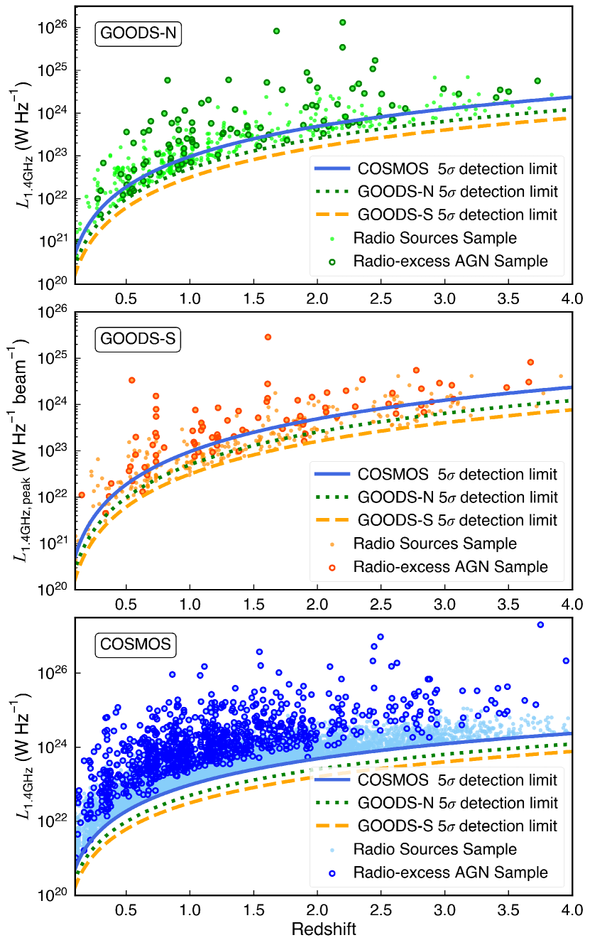
where is the luminosity distance (in the unit of meter), is the redshift, is the observed frequency (in the unit of GHz), and is the observed integrated flux densities at the observed frequency (Ceraj et al., 2018). For the GOODS-N field, we use the observed 1.4 GHz flux to calculate the rest-frame 1.4 GHz luminosity, while for the GOODS-S and COSMOS/UltraVISTA fields, we use the observed flux at 3 GHz. We show the distribution of rest-frame 1.4 GHz luminosity of our Radio Sources Sample with redshift in Fig. 2.
3.3 Stellar mass and UVJ magnitude
For the All Galaxies Sample in the GOODS-N field, their stellar masses and rest-frame UVJ magnitudes are derived from Barro et al. (2019) where stellar masses are estimated by SED fitting with the codes FAST (Kriek et al., 2009) and Synthesizer (Pérez-González et al., 2005, 2008), and rest-frame UVJ luminosities are estimated by EAZY (Brammer et al., 2008). For the All Galaxies Sample in the GOODS-S field, their stellar masses and rest-frame UVJ luminosities are estimated by the FAST from Santini et al. (2015) and EAZY from Straatman et al. (2016), respectively. For the All Galaxies Sample in the COSMOS/UltraVISTA field, their stellar masses and rest-frame UVJ magnitudes are derived from Weaver et al. (2022) where stellar masses are estimated by LePhare (Arnouts et al., 2002; Ilbert et al., 2006) and rest-frame UVJ luminosities are estimated by EAZY (Brammer et al., 2008). Our work and these aforementioned works used the same Chabrier (2003) IMF. In addition, to examine whether the above different methods will bring measurement bias for stellar mass, we also compare stellar masses given by the above methods () with those obtained by the broadband SED fitting (; see details in Appendix A for the GOODS fields and see details in Jin et al. 2018 for the COSMOS field). The logarithm of the ratio between and () is around dex. This result indicates that different methods give a consistent measurements for stellar mass. Given that only the Radio Sources Sample and Radio-excess AGN Sample have available broadband SED fitting results while the All Galaxies Sample do not have these measures, we use the stellar mass measured by FAST or LePhare in this work.
3.4 Galaxy type: SFGs and QGs
Color-magnitude or color-color criteria are an effective method to select SFGs and QGs, which does not require accurate measurements for star formation rate and stellar mass (e.g., Williams et al., 2009). In this work, we use UVJ selection criteria in Schreiber et al. (2015) to separate all our samples into SFGs and QGs at all redshift and stellar masses:
| (2) |
| (3) |
4 Radio-excess AGN
The excess radio emission from AGNs will make these types of sources deviate from the IRRC of SFGs. Therefore, AGN activities can be identified by these excess radio emission. Following Helou et al. (1985), we define the logarithmic ratio between total IR emission (8–1000 m; TIR) and radio emission as
| (4) |
where is the total IR luminosity and is the frequency at the center of FIR band (). In this work, we consider a broad redshift range from 0.1 to 4, which are divided into 6 redshift bins: , , , , , and . In this section, we focus on the Radio Sources Sample and then use distribution to select AGNs with excess radio emission which are called as radio-excess AGNs hereafter.
4.1 distribution and radio-excess AGN selection
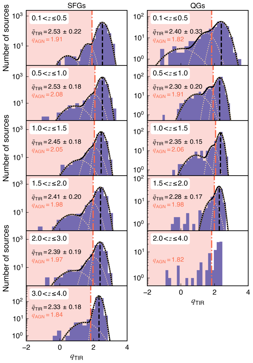
In this work we merge the radio sources in the GOODS-N, GOODS-S, and COSMOS/UltraVISTA fields together according to the following reasons. (1) Source numbers in each redshift bin for the GOODS-N and GOODS-S fields are small, which may result in a large uncertainty in determining the AGN selection threshold. (2) In each redshift bin, distributions in the GOODS-N, GOODS-S, and COSMOS fields have similar distributions and values (see Fig. D.4). The distribution consists of a gaussian component peaked at and an extended tail towards lower , which is consistent with previous works (e.g., Del Moro et al., 2013). The gaussian component is attributed to the IRRC of SFGs, while the extended tail is thought to be associated with the extra radio emission from AGN. Although the GOODS-S field has a slightly lower than the other two fields, it may not have a significant impact on the results (see details in Section 4.2). Therefore, to ensure the same selection criteria and reduce the uncertainty of the AGN selection threshold, we combine the data from the three fields together. The consistent radio luminosity functions among these three fields also indicate that our selection method is plausible (see details in Section 5). Next we analyze the distribution in SFGs and QGs, respectively.
For both SFGs and QGs, their entire distribution can be described by multiple gaussian models (see the yellow dotted curves in Fig. 3). We used -test probability at 95% confidence level to decide how many models are required. The final best-fit model are shown in Fig. 3 with black solid curves. As we mentioned before, the highest gaussian peak and the extended low- tail are thought to be contributed by SFGs and AGNs, respectively. Therefore, here we define the cross point between the highest gaussian and the second highest gaussian components as the threshold to separate the SFGs and radio-excess AGNs (see the values and red dash-dotted lines in Fig. 3). It means that a radio source will be selected as a radio-excess AGN if its value is lower than this cross point (). It is worth noting that the distributions of QGs also show a highest peak similar to SFGs. However, QGs are not expected to have this peak due to little or no star formation. One possible reason may be that UVJ color selection might classify part of massive SFGs with relatively lower star formation rate (SFR) as QGs (Popesso et al., 2023). We also found that nearly half of UVJ-selected QGs (without AGN) in the Radio Sources Sample locate very close to the dividing line in the UVJ diagram, which indicates that UVJ selection might not accurately classify these sources. QGs in the All Galaxies Sample and radio-excess AGNs hosted by QGs do not have this problem. This may explain why QGs show a highest peak in Fig. 3. In addition, the differential between the second highest and the third highest gaussian component in the distribution might be associated with different types of radio AGNs, which is beyond the scope of this work and will be studied in our future works.
Finally, we selected 1162 radio-excess AGNs at as our Radio-excess AGN Sample which contains 109 sources in the GOODS-N field, 83 sources in the GOODS-S field, and 970 sources in the COSMOS/UltraVISTA field (see circles with colored edges in Fig. 2).
4.2 evolution
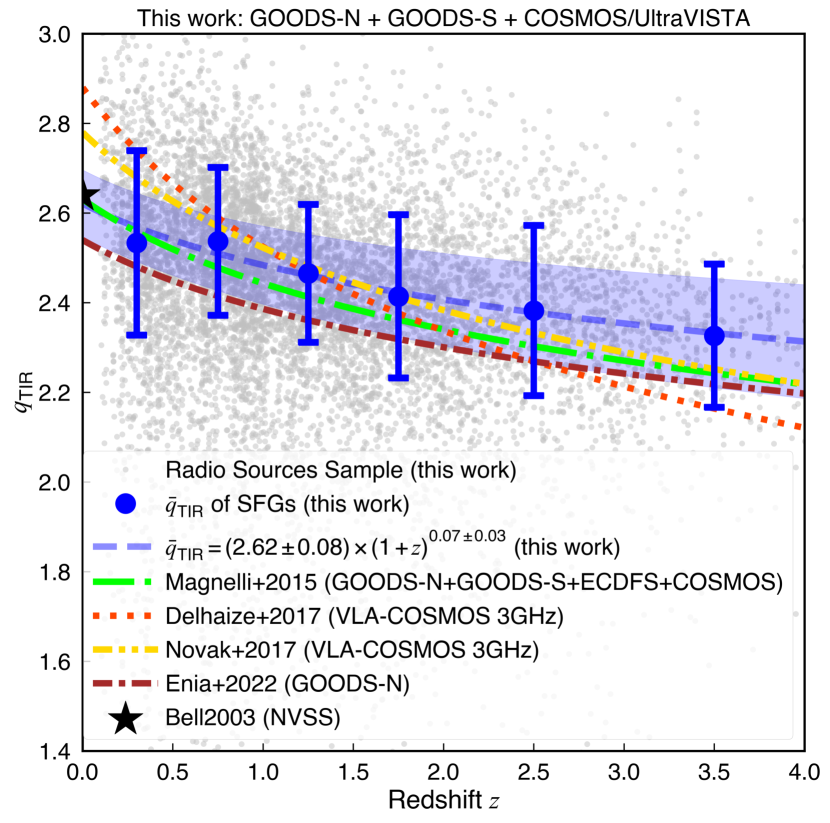
As Fig. 4 shows, presents a weak evolution with redshift, which is in the form of
| (5) |
Our result is almost consistent with previous works (see Fig. 4; Bell, 2003; Magnelli et al., 2015; Delhaize et al., 2017; Novak et al., 2017; Enia et al., 2022). Bell (2003) obtained value for SFGs in the local universe. Magnelli et al. (2015) combined data from multiple fields of the GOODS-N, GOODS-S, ECDFS, and COSMOS up to with rms noises larger than 3.9 at 1.4 GHz. Delhaize et al. (2017) and Novak et al. (2017) both used the VLA-COSMOS 3 GHz project but used different source selection criteria. Enia et al. (2022) focused on SFGs in the GOODS-N field. Compared to their works, we use simultaneously deeper and larger radio surveys, and more precise IR luminosity based on de-blended IR photometry. The slight difference between our results and previous works might be due to the different selection method for sources. In addition, the averaged standard deviation (1 error of in Fig. 4) of distribution for SFGs is around 0.18 which is consistent with the previous works (e.g., Del Moro et al., 2013).
More recently, Delvecchio et al. (2021) found that the IRRC of SFGs strongly depends on stellar mass (), while An et al. (2021) found a weak dependence. To examine whether considering -dependence or not affects our results, we make some simple tests. For the Radio Sources Sample in the COSMOS/UltraVISTA field, at , is around 2.55 and 2.53 for low-mass() and high-mass () SFGs, respectively. For the Radio Sources Sample in the GOODS-N field, at , is around 2.56 and 2.51 for low-mass () and high-mass () SFGs, respectively. For the Radio Sources Sample in the GOODS-S field, at , is around 2.50 and 2.33 for low-mass () and high-mass () SFGs, respectively. These results indicate that for most of our samples (GOODS-N and COSMOS/UltraVISTA fields), of SFGs shows a weak dependence on stellar mass, while of SFGs in the GOODS-S field show a decreasing trend towards larger stellar mass, which is consistent with the result in Delvecchio et al. (2021). The different trend in the GOODS-S field may explain why the GOODS-S field show a different distribution comparing to the other two fields (see Fig. D.4). Even so, this difference does not have a significant effect on our final results. On the one hand, SFGs (without AGNs) of the Radio Sources Sample in the GOODS-S field are not included in the subsequent studies (see details in Section 5.1). One the other hand, the classification purity corrections for the Radio-excess AGN Sample are also performed for each field (see details in Appendix D). Combining these results, disregarding the -dependent IRRC may have no significant effect on our results.
5 Radio luminosity function and their cosmic evolution
In this section, we will construct radio luminosity function (RLF) for SFGs and radio-excess AGNs which are separated in Section 4. Firstly, we estimate the combined 1.4 GHz RLF from the GOODS-N, GOODS-S, and COSMOS/UltraVISTA fields in Section 5.1. We then show the fitting procedures and results for the evolution of SFG RLFs (see Section 5.2) and AGN RLFs (see Section 5.3), respectively. In this work we do not consider the star-formation contamination for the 1.4 GHz radio luminosity of AGN. We have verified that for most of our Radio-excess AGN Sample, radio luminosity from the star formation is not significant compared to luminosity from AGN.
5.1 Construct RLF out to
Using the 1/ method (Schmidt, 1968), RLF in each 1.4 GHz luminosity bin and each redshift bin is calculated by
| (6) |
where is the size of the 1.4 GHz luminosity bin, is the observed area (171 arcmin2 for the GOODS-N and GOODS-S fields, and 1.5 degree2 for the COSMOS/UltraVISTA field), is the co-moving volume of the th source that is defined as , and is the completeness and bias correction factor of the th source. Further, is the co-moving volume at the maximum redshift where the th source can be observed given the 1.4 GHz flux detection limit (the maximum value of is equal to the upper limit of each redshift bin) and is the co-moving volume at the lower boundary of each redshift bin. The parameter is the flux density completeness of our catalogs which takes into account the effects of sensitivity limit. For sources in the COSMOS and GOODS-N fields, the completeness and bias corrections are estimated by Monte Carlo simulations where mock sources are inserted in and retrieved from the mosaic (see details in Smolčić et al., 2017b; Enia et al., 2022). For each source in the GOODS-S field, for simplicity, is estimated by the proportion of the area occupied by the sensitivity range which the peak radio flux of each source corresponds to. Specifically, the sensitivity contour map of the 3 GHz VLA image in the GOODS-S field can be shown as a series of concentric circles centered on the image center. The innermost circle has the highest sensitivity and sensitivity decreases gradually from the inside out ( value increases gradually). If one source has the peak radio flux larger than the of the th circle but lower than that of the ()th circle, its is calculated by the area of the th circle as a percentage of the total image area. The uncertainty of RLF in each luminosity bin and each redshift bin can be defined as
| (7) |
We used Equations 6 and 7 to calculate RLFs and their uncertainties for the sources in the GOODS-N, GOODS-S, and COSMOS/UltraVISTA, respectively (see Fig. B.2). For both SFGs and radio-excess AGNs, RLFs in these fields present generally consistent results. However, it is difficult to make completeness corrections for the GOODS-S field at the faint end. Thus, completeness corrections based on Monte Carlo simulations may be required, which is beyond the scope of this work. Therefore, for simplicity, we only utilize the observational data from the GOODS-N and COSMOS/UltraVISTA fields to calculate the RLF of SFGs, while for AGNs, all the data from the GOODS-N, GOODS-S, and COSMOS/UltraVISTA fields are considered. It is due to that AGN usually have higher radio luminosities which are less affected by the completeness correction. In order to well constrain the RLFs, in the following sections we use the averaged SFG RLFs in the GOODS-N and COSMOS/UltraVISTA fields, and use the averaged AGN RLFs in the three fields to make further ananlysis (see Fig. 5). In addition, we also correct the classification purity for the radio-excess AGN in these three fields (see details in Section D).
5.2 Fit the evolution of the SFG RLF
We assume a modified-Schechter function (Saunders et al., 1990; Smolčić et al., 2009; Gruppioni et al., 2013; Novak et al., 2017) to describe the SFG RLF. The local RLF of SFGs (Novak et al., 2017) is defined as
| (8) |
where is the turnover position of the local SFG RLF, is the local turnover normalization, and and are used to fit the distribution in the faint and bright ends, respectively.
SFG RLFs have been shown to evolve with redshift (e.g., Novak et al., 2017; Ocran et al., 2020; Cochrane et al., 2023). Given that it is difficult to simultaneously constrain the evolutions of all the parameters, we fix the and at all cosmic times to those of the local RLF (Novak et al., 2017) in the fit. It means that we assume an unchanged RLF shape at all cosmic times, and only allow the turnover position () and turnover normalization () to change with redshift. In reality, and might change with redshift.
Both evolution and evolution can be described by a simple power law:
| (9) |
and
| (10) |
respectively. Therefore, the redshift-evolved SFG RLF (luminosity and density evolution; hereafter “LDE”) is defined as
| (11) |
where is the parameter of pure density evolution (hereafter “PDE”; vertical shift of RLF), is the parameter of pure luminosity evolution (hereafter “PLE”; horizontal shift of RLF), and is the local SFG RLF given by Eq. 8. If we assume that there is no evolution with redshift for and only evolves with redshift (), we can define a SFG PLE model as
| (12) |
Similarly, SFG PDE model only allows to evolve with redshift (), which is defined as
| (13) |
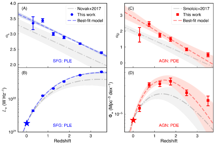
Then we used the Markov chain Monte Carlo (MCMC) algorithm in the Python package emcee (Foreman-Mackey et al., 2013) to fit the data in Table 4 with the above three models. The averaged reduced over all the redshift bins of the best-fit LDE, PLE, and PDE models are 4.0, 6.5, and 738.2, respectively. Firstly, we ignored the PDE model because it has the worst fit to the observational data. The best-fit LDE and PLE models show significant differences at higher redshift () where our data points are mainly in the bright end of RLF. This will result in degeneracy in estimation of and , preventing a precise calculation to the turnover position and turnover normalization. Therefore, for simplicity, we only consider the PLE model (see Equation 12) here.
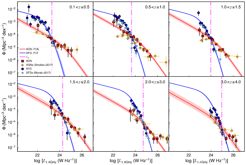
The best-fit of the PLE model in each redshift bin is summarized in Table 1. shows an evolution with redshift, which can be described by . We obtain the best-fit results with and (see Panel A of Fig 6), which are also summarized in Table 1. The turnover position is estimated by Equation 9, which is also listed in Table 1. Our results are generally consistent with those in Novak et al. (2017) with the VLA-COSMOS 3 GHz project (see Fig. 5 and Fig. 6), although our results show a slightly larger (see Panel A of Fig. 6) and a slightly larger (see Panel B of Fig. 6), which may be due to the different selection criteria adopted for radio SFGs.
5.3 Fit the evolution of the AGN RLF
The AGN RLF can be assumed as a double power-law shape (Mauch & Sadler, 2007). The local RLF of AGN (Mauch & Sadler, 2007) is defined as
| (14) |
where is the turnover normalization of the local AGN RLF, is the local turnover position, and are the indices at the bright and faint end, respectively.
Similar to the SFG RLF, we assume that AGN RLF has an unchanged shape at all cosmic times. Thus, similar to Equations 11 – 13, LDE, PLE, and PDE models to describe AGN RLFs can be defined as
| (15) |
| (16) |
| (17) |
respectively. We also use the emcee package to fit the observational data for radio-excess AGNs in Table 5 with these three models. The averaged reduced over all the redshift bins of the best-fit LDE, PDE, and PLE models are 2.02, 1.75, and 2.27, respectively. Here we only consider the PDE model (see Equation 16) which has the best fit to the data.
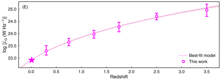
The best-fit of the PDE model in each redshift bin is also summarized in Table 1, which also shows a redshift evolution in a form of . The best-fit and are and , respectively (also see Table 1). As we assumed an unchanged AGN RLF shape and a pure density evolution, the evolution of (calculated by Equation 10) with redshift can simply represent the number density distribution of AGN, which peaked at (see Panel D of Fig. 6). Our result is generally consistent with that in Smolčić et al. (2017a) based on the VLA-COSMOS 3 GHz project (see Fig. 5 and Fig. 6), and consistent with the AGN accretion rate density history obtained with X-ray surveys (Aird et al., 2010, and references therein).
We also study the RLF of the Radio-excess AGN Sample hosted by different galaxy populations (SFGs and QGs; see Fig. C.3). At , the entire radio-excess AGNs are mainly dominated by the sources hosted by QGs, while radio-excess AGNs hosted by SFGs only have a comparable space densities at the faint end. At , the space densities of radio-excess AGNs hosted by QGs decrease towards higher redshift, while radio-excess AGNs hosted by SFGs show an opposite evolution trend. In addition, radio-excess AGNs hosted by SFGs completely dominate those hosted by QGs at . These trends are consistent with those for low-excitation radio galaxies in Kondapally et al. (2022). Although we focus on different types of radio-AGNs, these consistent trends indicate that the activities of central SMBHs may depend on the fuelling mechanisms of their host galaxies. In Section 6, we will further investigate this topic through studying the probability of radio-excess AGNs hosted by different galaxy populations.
| \addstackgap[.5] | SFG (PLE) | Radio-excess AGN (PDE) | |||
|---|---|---|---|---|---|
| Redshift bin | |||||
| \addstackgap[.5] | |||||
| \addstackgap[.5] Relation | |||||
| \addstackgap[.5] Best-fit parameters | |||||
5.4 Crossover luminosity between SFG RLF and AGN RLF
The comparison between the SFG RLF and AGN RLF shows that AGNs will dominate the radio populations beyond a certain luminosity (hereafter turnover luminosity ; see the magenta dash-dotted lines in Fig. 5). In the local universe, this crossover luminosity is around , which is usually used to select RL AGNs (e.g., Best et al., 2005; Kukreti et al., 2023). Towards higher redshift, given that both SFG RLFs and AGN RLFs show evolutions with redshift, this crossover luminosity will not be expected to be constant at all cosmic time. Our results indicate that the redshift evolution of this crossover luminosity can be described by
| (18) |
where is the crossover luminosity in the local universe, is the evolution index of the crossover luminosity. Here, , is obtained by the cross point between the local SFG RLF (Novak et al., 2017) and local AGN RLF (Mauch & Sadler, 2007). Further, also shows a weak evolution with redshift:
| (19) |
These results provide us another way to select powerful radio AGNs at different redshift through solely radio survey. It means that if IR data are not available, a radio source at redshift can be selected as a radio AGN when its 1.4 GHz radio luminosity is larger than . This crossover luminosity describes a luminosity threshold where radio-AGNs begin to dominate entire radio populations, which shows an increasing trend towards higher redshift. This result is also consistent with those from previous works (e.g., McAlpine et al., 2013), and also agrees with the threshold used in radio-AGN selections (e.g., Magliocchetti et al., 2017).
6 The probability of hosting a radio-excess AGN in SFGs and QGs
In this section, we aim to study the probability of different galaxy populations hosting a radio-excess AGN. Here we use the combined All Galaxies Sample (see Section 2 and Fig. 1) and combined Radio-excess AGN Sample (see Section 4 and Fig. 1) in the GOODS-N, GOODS-S, and COSMOS/UltraVISTA fields. The All Galaxies Sample and the host galaxies of the Radio-excess AGN Sample had been divided into SFGs and QGs according to the UVJ selection method (see Section 3.4). In Sections 6.1 and 6.2, we use the observational data to calculate the probability of a SFG or a QG with the stellar mass and at redshift hosting a radio-excess AGN with the 1.4 GHz luminosity in each redshift bin. In Section 6.3, we use the method of Aird et al. (2012) to quantitatively calculate the probability of a SFG or a QG hosting a radio-excess AGN as a function of stellar mass, radio luminosity, and redshift. This method is based on the maximum-likelihood approach, which does not require data binning for stellar mass, luminosity, and redshift (Aird et al., 2012).
6.1 Calculate the probability for observational data
In order to conveniently compare the data and the best-fit model, we divided our All Galaxies Sample and Radio-excess AGN Sample into 6 redshift bins (same as the redshift bins in Section 4). Within each redshift bin, we subdivided our All Galaxies Sample and Radio-excess AGN Sample into different stellar mass bins. The conditional probability density function describes the probability of a galaxy with stellar mass and at redshift hosting a radio-excess AGN with 1.4 GHz luminosity . Following Aird et al. (2012), here is defined as the probability density per logarithmic luminosity interval (units are dex-1). Thus, can be converted to AGN fraction () according to
| (20) |
Here is defined as the fraction of galaxies with stellar mass and at redshift that host a radio-excess AGN, is the lower limit of the radio luminosity. For the combined observational data from the GOODS-N, GOODS-S, and COSMOS/UltraVISTA fields, in each redshift bin, in the th stellar mass bin and the th luminosity bin is defined by
| (21) |
where is the number of the Radio-excess AGN Sample in the th stellar mass bin and the th luminosity bin, is the number of the All Galaxies Sample in the th stellar mass bin, and is the width of the th luminosity bin. It is worth stating that when calculating the probability of SFGs (or QGs, or all galaxies) hosting a radio-excess AGN, here refers to all the radio-excess AGNs hosted by SFGs (or QGs, or all galaxies) and refers to all the SFGs (or QGs, or all galaxies) in the All Galaxies Sample. The estimates of for SFGs in 6 redshift bins are shown as colored symbols in Fig. E.5 and Fig. E.6. The radio-excess AGNs in both QGs and all galaxies exhibit similar trends to SFGs, so we do not show their details here. The probability of a galaxy hosting a radio-excess AGN with a given increases with at all redshift bins (see Fig. E.5), which is consistent with the previous works (e.g., Best et al., 2005; Sabater et al., 2019). The probability of a galaxy with a given hosting a radio-excess AGN decreases with , which is also consistent with previous works (e.g., Best et al., 2005). These trends of radio-excess AGNs in this work are consistent with those of X-ray AGNs (e.g., Haggard et al., 2010; Aird et al., 2012; Wang et al., 2017).
6.2 Simple fits in each redshift bin
To quantitatively study the trends of , we apply fits to the results calculated by Equation 21 (see the data points in Fig. E.5 and Fig. E.6). Next we take the analysis for SFGs as an example to show the detailed analysis procedures. At each fixed , we assume a simple power-law relation for as a function of ,
| (22) |
where and are the intercept and slope of the relation, respectively. The best-fit values for and in each bin and each redshift bin are presented in the right column of Fig. E.5. The averaged best-fit reduced- over all the redshift bins and all the bins is 1.22. In all redshift bins, the intercept decreases with larger , while the slope does not show significant changes. Similarly, for each fixed , as a function of can be defined as
| (23) |
where and are the intercept and slope of the relation, respectively. The best-fit parameters in each bin and each redshift bin are shown in the right column of Fig. E.6. The averaged best-fit reduced- over all the redshift bins and all the bins is 1.76. In all redshift bins, the intercept decreases with higher , while the slope nearly keeps constant. These results indicate that the slope (or the slope ) of as a function of (or ) is independent of (or ). QGs and all galaxies show similar trends but different best-fit parameters comparing to SFGs. Given that we mainly focus on the trends in this section, for brevity, we do not discuss their results in details here. The main differences among different galaxy populations are discussed in Section 6.3.4 and shown in Fig. 7.
6.3 Redshift evolution
The above analysis depends on the bin size of and , which cannot utilize all the information of each individual galaxy and may bias to the bin size. Therefore, next we utilize the maximum likelihood fitting approach in Aird et al. (2012) to measure the dependence of on both and . At first, in Section 6.3.1, we introduce the fitting approach applied to our samples. Then we test this approach in each redshift bin in Section 6.3.2. Finally, in Section 6.3.3, we apply this approach incorporating the redshift evolution in order to remove the effects brought by the redshift binning.
6.3.1 Maximum-likelihood fitting
According to the results in Section 6.2, the slope (or ) in Equation 22 (or 23) of as a function of (or ) is independent of (or ). It means that at a fixed redshift can be expressed as a separable function of and in the form of
| (24) |
where the scaling factor is set to , the scaling factor is set to , is the normalization, and are indices. The best-fit parameters are found through maximizing the log-likelihood function,
| (25) |
where is the number of radio-excess AGNs in the GOODS-N, GOODS-S, and COSMOS/UltraVISTA fields in the th redshift bin, is the probability of a galaxy with stellar mass hosting a radio-excess AGN with 1.4 GHz luminosity :
| (26) |
The expected number of radio-excess AGNs, , is defined as
| (27) | ||||
where , , and are the numbers of galaxies in the th redshift bin for the GOODS-N, GOODS-S, COSMOS/UltraVISTA fields, respectively. of the GOODS-N field () corresponds to the detection limit of the radio survey at redshift (see Fig. 2), while for the GOODS-S () and COSMOS () fields, it corresponds to the threshold for correcting the AGN classification purity (see details in Appendix D). The error of each model parameter is estimated by the maximum projection of where according to Aird et al. (2012).
6.3.2 Results in each redshift bin
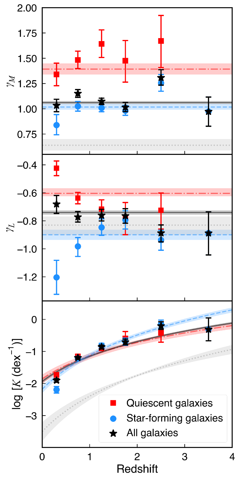
In each redshift bin, we use the above maximum-likelihood fitting approach to constrain for SFGs, QGs, and all galaxies. The best-fit values for , , and in each redshift bin are shown in the form of colored symbols in Fig. 7. For both SFGs and QGs, we find that and almost keep constant at all redshift bins except at (see detailed discussions in Section 6.3.3). For all galaxies, and do not show any significant changes with redshift (), which is consistent with the trends of X-ray AGNs in Aird et al. (2012) at . For SFGs, QGs and all galaxies, the normalization significantly increases with redshift. In addition, SFGs and QGs show significantly different , , and , which will be discussed in details in Section 6.3.4. Overall, the probability of a galaxy with a given stellar mass hosting a radio-excess AGN with a given radio luminosity increases towards higher redshift. This indicates higher AGN activities and potentially more significant AGN feedbacks towards higher redshift.
6.3.3 Incorporating redshift evolution into the maximum-likelihood fitting
According to the results of Section 6.3.2, both and are nearly constant over the entire redshift range, which indicates that the redshift evolution of can be assumed to be independent of and . Only the normalization shows an evolution with redshift, so incorporating the redshift evolution for with a simple power-law can be rewritten as
| (28) |
where the scaling factor is set to be 2.0 (median of the redshift range for our sample), is the overall normalization. Thus,
| (29) |
Then we modify in Equations 25–27 with Equation 28 to perform maximum-likelihood fitting over the entire redshift range (). The best-fit parameters are listed in Table 2 and plotted in Fig. 7 as the colored lines. The redshift evolution model over the entire redshift range is almost consistent with the result obtained in each redshift bin (colored symbols in Fig. 7).
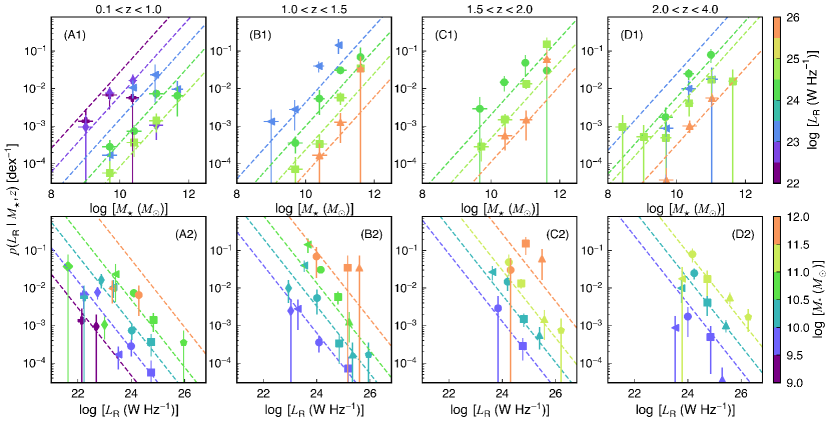
To compare the model with the observational data, we use the method of Aird et al. (2012) (see Equation 14 in their paper) to scale the observed radio-excess AGN number () by the expected number estimated by the model () in each redshift bin (see Equation 28). Overall, the binned estimates for the observational data in each redshift bin are well described by the best-fit model obtained with maximum-likelihood fitting over the entire redshift range (see results for SFGs in Fig. 8, for QGs in Fig. F.7, for all galaxies in Fig. F.8). However, the best-fit model cannot fully explain the data in the following cases: low-luminosity radio-excess AGN in SFGs at (; see Panel A1 in Fig. 8) and at (; see Panel D1 in Fig. 8), radio-excess AGN in massive SFGs () at (see Panels A2 in Fig. 8), radio-excess AGN in low-mass QGs () at (see Panels A2 in Fig. F.7, repectively). The following reasons might explain the slight differences between observational data and model predictions. In the analysis, we assume that (or ) is independent of (or ) and redshift (see Sections 6.2 and 6.3.2). On the one hand, a mild dependence of (or ) on (or ) cannot be fully ruled out. In addition, may be different between low-mass and high-mass galaxies (Williams & Röttgering, 2015; Zhu et al., 2023), while may also change from low-luminosity to high-luminosity populations (Best et al., 2005). On the other hand, a weak evolution of both and with redshift might exist (see colored symbols in Fig. 7). Some works had found that decreases from the local universe to (Williams & Röttgering, 2015; Zhu et al., 2023), while Kondapally et al. (2022) found a weak evolution with redshift. Even so, on the whole our model can still well describe the redshift evolution of radio-excess AGN fraction across the entire redshift range.
| \addstackgap[.5] Type | ||||
|---|---|---|---|---|
| \addstackgap[.5] SFG | ||||
| QG | ||||
| All |
6.3.4 Quantitative relation of radio-excess AGN fraction in SFGs and QGs
To sum up, we obtain quantitative relations for the probability of SFGs, QGs, or all galaxies hosting a radio-excess AGN as a function of , , and redshift, respectively:
| (30) | ||||
where is set to , is set to , and is set to 2.0. SFGs and QGs have significantly different evolution trends for radio-excess AGN fraction (also see Fig. 7). QGs have larger and than SFGs, which indicates that radio-excess AGNs in QGs prefer to reside in more massive galaxies with higher radio luminosity compared to those in SFGs. Both SFGs and QGs have an increasing radio-excess AGN fraction with redshift (see Fig. 7). SFGs show a larger than QGs (see Table 2), which implies that radio-excess AGN fractions in SFGs increase more rapidly towards higher redshift than those in QGs.
7 Discussion
7.1 Comparison with previous works
As Equation 30 shows, we obtain a smaller () than that in Best et al. (2005) (; ). Our result is consistent with that in Williams & Röttgering (2015) at (), while their results showed a decreasing trend from the local universe () to . Zhu et al. (2023) also found a decreasing stellar-mass dependence from to . In addition, the dependence of radio-AGN fraction on the stellar mass may change when (Williams & Röttgering, 2015; Zhu et al., 2023). The differences between our and their results may be due to the different radio-AGN selections and different calculation methods. Previous works usually focused on powerful radio-AGNs (), while our sample additionally includes some faint radio-AGNs with . Moreover, the different evolution trends of radio-AGN in SFGs and QGs indicate that disregarding the galaxy types may have a non-negligible effect on statistical results. Kondapally et al. (2022) proposed for the first time a radio-AGNs study for QGs and SFGs seperately. They found that low-excitation radio galaxies in QGs have a larger () than those in SFGs (). We found a similar trend but lower values than their results ( for QGs and for SFGs in our work). One possible reason for this difference may be that we focus on different types of radio-AGNs comparing to Kondapally et al. (2022). Our results show that has no significant evolution with redshift at , which is consistent with that found in Kondapally et al. (2022) at .
Given that we use the same calculation method as Aird et al. (2012) (see details in Section 6.3), we also compare the results for radio-excess AGNs with those for X-ray AGNs from Aird et al. (2012) which are plotted as gray dotted lines in Fig. 7. Comparing to X-ray AGNs (Aird et al., 2012), evolutions of radio-excess AGN fraction (see black solid lines in Fig. 7) have a larger , which indicates that radio-excess AGNs tend to reside in more massive galaxies (see Fig. 7). X-ray AGN fractions in red sequence galaxies exhibit a more rapid redshift evolution than those in blue cloud galaxies (Aird et al., 2012; Wang et al., 2017), while radio-excess AGNs fraction in SFGs increases more rapidly towards higher redshift than those in QGs. These different evolution trends between radio-excess AGNs and X-ray AGNs suggest that black holes with different accretion states may influence their host galaxies in different modes.
In addition, we also examine whether -dependent IRRC (Delvecchio et al., 2021) affects the results about the probability of hosting a radio-excess AGN. Following van der Vlugt et al. (2022), we select radio-excess AGNs with deviating more than from the -dependent IRRC of Delvecchio et al. (2021). Then we recalculate the probability of a radio-excess AGN hosted by SFGs using Equation 28 (see the dark blue region in Fig. G.9) which is consistent with the results based on the radio-excess-AGN selection method in Section 4 (see the green region in Fig. G.9). This result indicates that using the -dependent IRRC (Delvecchio et al., 2021) does not alter the results in this work.
7.2 Physical origins of radio-excess AGN fractions
In order to investigate the relation between the radio-excess AGN fraction and physical properties of the central engine, we utilize the black hole fundamental plane (Merloni et al., 2003; Bonchi et al., 2013) to convert the as a function of X-ray luminosity and black hole mass. The best-fit model of for SFGs and QGs (see details in Section 6.3.3 and Equation 30) can be simplified as the scaling relations in the form of and , respectively. Then we use the black hole fundamental plane (BHFP) of from Bonchi et al. (2013) ( is the intrinsic 2–10 keV X-ray luminosity and is the black hole mass). Bonchi et al. (2013) obtained the BHFP based on X-ray-selected AGNs with unabsorbed larger than at . We have verified that nearly 20% of our Radio-excess AGN Sample at have X-ray counterparts, most of which have larger than . Therefore, it is feasible to apply the BHFP from Bonchi et al. (2013) on our sample. We assume a constant 2–10 keV X-ray bolometric correction to convert X-ray luminosity into bolometric luminosity (), and a constant scaling between black hole mass and stellar mass of (Marconi & Hunt, 2003). Then we calculate the Eddington ratios using . Combining these relations, Equation 30 can be rewritten as
| (31) | ||||
These relations indicate that the evolution of radio-excess AGN fraction in SFGs is determined by the Eddington ratio and redshift. The evolution of radio-excess AGN fraction in QGs depends on Eddington ratio, redshift, and also stellar mass (or black hole mass). It is worth noting that the radio luminosity of the BHFP refers to the radio emission from the core, but radio data used in this work cannot resolve the radio emission from core and lobe separately for most sources in our sample. Given that most of radio AGN () may be consistent with point sources rather than extended morphologies (Barišić et al., 2017), using total radio luminosity here might not make a significant effect on our result.
Radio-excess AGN fraction might be related to the growing states of black holes. Kauffmann & Heckman (2009) used a large AGN sample from Sloan Digital Sky Survey to study the black hole growth in nearby galaxies. They suggested two different regimes of black hole growth in the local universe, which had been confirmed by studies with X-ray AGNs (Aird et al., 2012; Wang et al., 2017). The first regime usually appears in galaxies with significant recent or ongoing star formations. In this regime, the distribution function of black hole accretion rate remains nearly constant (peaked at a few percent of the Eddington ratio), and independent of stellar velocity dispersion and black hole mass. Thus, Kauffmann & Heckman (2009) argued that the accretion onto the black hole is regulated by the feedback processes associated with the black hole itself (such as winds or jets) rather than the supply of gas from the host galaxies. However, the feedback processes may have an impact on gas supply, which will affect the growth of BH by accreting gas. The second regime usually appears in galaxies with little or no star formation. In this regime, the distribution function of black hole accretion rate depends on both black hole mass and the age of stellar populations. Thus, Kauffmann & Heckman (2009) thought that black holes during this period may be growing through stellar mass loss. However, other BH growth modes among old and massive galaxies may also exist, such as accreting the hot halo gas (Kondapally et al., 2022; Ni et al., 2023).
Our results show that radio-excess AGN fraction in SFGs only depends on the accretion states of black holes (Eddington ratio). It supports the scenario of the first regime that black holes regulate their own growth during star-forming periods of host galaxies. Galaxies may run out their gas to become a QG which corresponds to the second regime. According to our results, radio-excess AGN fraction in QGs depends on the accreting states of black holes and the properties of host galaxies simultaneously. It implies that host galaxies begin to regulate the black hole growth, which is also consistent with the scenario in the second regime. Therefore, our results also support the arguments about black hole growth in Kauffmann & Heckman (2009): if host galaxies have plentiful cold gas to supply, central black holes regulate their own growth, when these gas runs out, the rate of stellar mass loss in host galaxies may begin to take significant effects on the black hole growth. However, other fuelling mechanisms, such as cooling of hot gas from haloes and galaxy mergers, may also play an important role in SMBH growth, which requires dynamical and environmental properties to make further investigation in the future.
8 Summary
Firstly we use the optical to MIR surveys to select a All Galaxies Sample with 500,000 sources at in GOODS-N, GOODS-S, COSMOS/UltraVISTA fields (totaling 1.6 degree2; Section 2). After cross-matching with the deep/large radio surveys (1.4 GHz or 3 GHz) in these fields, we select 7878 radio sources with S/N of radio flux at as our Radio Sources Sample (Section 2). Combining with the de-blended IR photometry in these fields, we calculate the infrared-radio ratio () distributions of these radio sources to select a Radio-excess AGN Sample with 1162 sources (Section 4.1). Next we subdivide all our samples into SFGs and QGs using the UVJ method. Based on the Radio Sources Sample, we construct 1.4 GHz radio luminosity functions (RLFs) for SFGs and radio-excess AGNs at (Section 5.1), respectively, and study their evolutions with redshift. Based on the All Galaxies Sample and Radio-excess AGN Sample, we further investigate the probability of different galaxies populations (SFGs and QGs) hosting a radio-excess AGN as a function of stellar mass, radio luminosity, and redshift. The main conclusions we have obtained are shown as follows.
-
1.
The value of SFGs shows a weak evolution with redshift: (Section 4.2), which is generally consistent with previous works.
- 2.
-
3.
The evolution of crossover luminosity between SFG RLFs and AGN RLFs is shown as , which can be used to select powerful radio AGNs at different redshifts through solely radio surveys (Section 5.4). This result also indicate a decreasing contribution of AGNs to entire radio populations towards higher redshift.
-
4.
The probability of a galaxy hosting a radio-excess AGN is shown as a function of stellar mass, radio luminosity, and redshift: for SFGs, for QGs (Section 6.3). It indicates that radio-excess AGNs in QGs prefer to reside in more massive galaxies with larger radio luminosity than those in SFGs. The fractions of radio-excess AGNs in both SFGs and QGs are increasing from the local universe to the higher redshift. In addition, this increasing trend in SFGs is more significant than in QGs.
-
5.
Combining with the black hole fundamental plane, we find that the probability of hosting a radio-AGNs is related to accretion states of BHs and redshift in SFGs, while in QGs, it also depends on BH (or galaxy) masses (Section 7.2). These results might support such a physical scenario: if host galaxies have plentiful cold gas to supply, central black holes regulate their own growth, when these gas runs out, the rate of stellar mass loss in host galaxies may begin to take significant effects on the black hole growth.
The above studies can lay the foundation for further investigation with the upcoming revolutionary radio facilities, such as Square Kilometer Array (SKA; Dewdney et al., 2009; Norris et al., 2013; McAlpine et al., 2015) and the Next Generation Very Large Array (ngVLA; Hughes et al., 2015).
Acknowledgements.
We thank the referee for constructive comments that greatly improved this paper. This work is supported by the National Natural Science Foundation of China (Project No. 12173017 and Key Project No. 12141301).References
- Aird et al. (2012) Aird, J., Coil, A. L., Moustakas, J., et al. 2012, ApJ, 746, 90
- Aird et al. (2010) Aird, J., Nandra, K., Laird, E. S., et al. 2010, MNRAS, 401, 2531
- Alberts et al. (2020) Alberts, S., Rujopakarn, W., Rieke, G. H., Jagannathan, P., & Nyland, K. 2020, ApJ, 901, 168
- An et al. (2021) An, F., Vaccari, M., Smail, I., et al. 2021, MNRAS, 507, 2643
- Appleton et al. (2004) Appleton, P. N., Fadda, D. T., Marleau, F. R., et al. 2004, ApJS, 154, 147
- Arnouts et al. (2002) Arnouts, S., Moscardini, L., Vanzella, E., et al. 2002, MNRAS, 329, 355
- Baldwin et al. (1981) Baldwin, J. A., Phillips, M. M., & Terlevich, R. 1981, PASP, 93, 5
- Bariuan et al. (2022) Bariuan, L. G. C., Snios, B., Sobolewska, M., Siemiginowska, A., & Schwartz, D. A. 2022, MNRAS, 513, 4673
- Barišić et al. (2017) Barišić, I., van der Wel, A., Bezanson, R., et al. 2017, ApJ, 847, 72
- Barro et al. (2019) Barro, G., Pérez-González, P. G., Cava, A., et al. 2019, ApJS, 243, 22
- Bell (2003) Bell, E. F. 2003, ApJ, 586, 794
- Best et al. (2005) Best, P. N., Kauffmann, G., Heckman, T. M., et al. 2005, MNRAS, 362, 25
- Best et al. (2023) Best, P. N., Kondapally, R., Williams, W. L., et al. 2023, MNRAS, 523, 1729
- Bonchi et al. (2013) Bonchi, A., La Franca, F., Melini, G., Bongiorno, A., & Fiore, F. 2013, MNRAS, 429, 1970
- Boquien et al. (2019) Boquien, M., Burgarella, D., Roehlly, Y., et al. 2019, A&A, 622, A103
- Brammer et al. (2008) Brammer, G. B., van Dokkum, P. G., & Coppi, P. 2008, ApJ, 686, 1503
- Brown et al. (2011) Brown, M. J. I., Jannuzi, B. T., Floyd, D. J. E., & Mould, J. R. 2011, ApJ, 731, L41
- Bruzual & Charlot (2003) Bruzual, G. & Charlot, S. 2003, MNRAS, 344, 1000
- Burgarella et al. (2005) Burgarella, D., Buat, V., & Iglesias-Páramo, J. 2005, MNRAS, 360, 1413
- Calistro Rivera et al. (2017) Calistro Rivera, G., Williams, W. L., Hardcastle, M. J., et al. 2017, MNRAS, 469, 3468
- Calzetti et al. (2000) Calzetti, D., Armus, L., Bohlin, R. C., et al. 2000, ApJ, 533, 682
- Ceraj et al. (2018) Ceraj, L., Smolčić, V., Delvecchio, I., et al. 2018, A&A, 620, A192
- Chabrier (2003) Chabrier, G. 2003, ApJ, 586, L133
- Cochrane et al. (2023) Cochrane, R. K., Kondapally, R., Best, P. N., et al. 2023, MNRAS, 523, 6082
- Condon (1992) Condon, J. J. 1992, ARA&A, 30, 575
- Condon & Dressel (1978) Condon, J. J. & Dressel, L. L. 1978, ApJ, 221, 456
- Condon et al. (2019) Condon, J. J., Matthews, A. M., & Broderick, J. J. 2019, ApJ, 872, 148
- Cowie et al. (2018) Cowie, L. L., González-López, J., Barger, A. J., et al. 2018, ApJ, 865, 106
- Dale et al. (2014) Dale, D. A., Helou, G., Magdis, G. E., et al. 2014, ApJ, 784, 83
- Davé et al. (2019) Davé, R., Anglés-Alcázar, D., Narayanan, D., et al. 2019, MNRAS, 486, 2827
- Del Moro et al. (2013) Del Moro, A., Alexander, D. M., Mullaney, J. R., et al. 2013, A&A, 549, A59
- Delhaize et al. (2017) Delhaize, J., Smolčić, V., Delvecchio, I., et al. 2017, A&A, 602, A4
- Delvecchio et al. (2022) Delvecchio, I., Daddi, E., Sargent, M. T., et al. 2022, A&A, 668, A81
- Delvecchio et al. (2021) Delvecchio, I., Daddi, E., Sargent, M. T., et al. 2021, A&A, 647, A123
- Delvecchio et al. (2017) Delvecchio, I., Smolčić, V., Zamorani, G., et al. 2017, A&A, 602, A3
- Dewdney et al. (2009) Dewdney, P. E., Hall, P. J., Schilizzi, R. T., & Lazio, T. J. L. W. 2009, IEEE Proceedings, 97, 1482
- Donley et al. (2012) Donley, J. L., Koekemoer, A. M., Brusa, M., et al. 2012, ApJ, 748, 142
- Donley et al. (2005) Donley, J. L., Rieke, G. H., Rigby, J. R., & Pérez-González, P. G. 2005, ApJ, 634, 169
- Donoso et al. (2009) Donoso, E., Best, P. N., & Kauffmann, G. 2009, MNRAS, 392, 617
- Donoso et al. (2010) Donoso, E., Li, C., Kauffmann, G., Best, P. N., & Heckman, T. M. 2010, MNRAS, 407, 1078
- Draine & Li (2007) Draine, B. T. & Li, A. 2007, ApJ, 657, 810
- Dubner & Giacani (2015) Dubner, G. & Giacani, E. 2015, A&A Rev., 23, 3
- Dullo et al. (2023) Dullo, B. T., Knapen, J. H., Beswick, R. J., et al. 2023, MNRAS, 522, 3412
- Enia et al. (2022) Enia, A., Talia, M., Pozzi, F., et al. 2022, ApJ, 927, 204
- Fabian (2012) Fabian, A. C. 2012, ARA&A, 50, 455
- Fiore et al. (2017) Fiore, F., Feruglio, C., Shankar, F., et al. 2017, A&A, 601, A143
- Foreman-Mackey et al. (2013) Foreman-Mackey, D., Hogg, D. W., Lang, D., & Goodman, J. 2013, PASP, 125, 306
- Franzen et al. (2021) Franzen, T. M. O., Seymour, N., Sadler, E. M., et al. 2021, PASA, 38, e041
- Gim et al. (2019) Gim, H. B., Yun, M. S., Owen, F. N., et al. 2019, ApJ, 875, 80
- Gómez-Guijarro et al. (2022) Gómez-Guijarro, C., Elbaz, D., Xiao, M., et al. 2022, A&A, 658, A43
- Grogin et al. (2011) Grogin, N. A., Kocevski, D. D., Faber, S. M., et al. 2011, ApJS, 197, 35
- Gruppioni et al. (2013) Gruppioni, C., Pozzi, F., Rodighiero, G., et al. 2013, MNRAS, 432, 23
- Guo et al. (2013) Guo, Y., Ferguson, H. C., Giavalisco, M., et al. 2013, ApJS, 207, 24
- Haggard et al. (2010) Haggard, D., Green, P. J., Anderson, S. F., et al. 2010, ApJ, 723, 1447
- Hardcastle & Croston (2020) Hardcastle, M. J. & Croston, J. H. 2020, New A Rev., 88, 101539
- Helou et al. (1985) Helou, G., Soifer, B. T., & Rowan-Robinson, M. 1985, ApJ, 298, L7
- Ho (2008) Ho, L. C. 2008, ARA&A, 46, 475
- Hughes et al. (2015) Hughes, A. M., Beasley, A., & Carilli, C. 2015, in IAU General Assembly, Vol. 29, 2255106
- Ilbert et al. (2006) Ilbert, O., Arnouts, S., McCracken, H. J., et al. 2006, A&A, 457, 841
- Ivison et al. (2010) Ivison, R. J., Magnelli, B., Ibar, E., et al. 2010, A&A, 518, L31
- Janssen et al. (2012) Janssen, R. M. J., Röttgering, H. J. A., Best, P. N., & Brinchmann, J. 2012, A&A, 541, A62
- Jin et al. (2018) Jin, S., Daddi, E., Liu, D., et al. 2018, ApJ, 864, 56
- Kauffmann & Heckman (2009) Kauffmann, G. & Heckman, T. M. 2009, MNRAS, 397, 135
- Kauffmann et al. (2003) Kauffmann, G., Heckman, T. M., Tremonti, C., et al. 2003, MNRAS, 346, 1055
- Kewley et al. (2013) Kewley, L. J., Maier, C., Yabe, K., et al. 2013, ApJ, 774, L10
- Koekemoer et al. (2011) Koekemoer, A. M., Faber, S. M., Ferguson, H. C., et al. 2011, ApJS, 197, 36
- Kolwa et al. (2019) Kolwa, S., Jarvis, M. J., McAlpine, K., & Heywood, I. 2019, MNRAS, 482, 5156
- Kondapally et al. (2022) Kondapally, R., Best, P. N., Cochrane, R. K., et al. 2022, MNRAS, 513, 3742
- Kondapally et al. (2023) Kondapally, R., Best, P. N., Raouf, M., et al. 2023, MNRAS, 523, 5292
- Kriek et al. (2009) Kriek, M., van Dokkum, P. G., Labbé, I., et al. 2009, ApJ, 700, 221
- Kukreti et al. (2023) Kukreti, P., Morganti, R., Tadhunter, C., & Santoro, F. 2023, arXiv e-prints, arXiv:2305.03725
- Lacy et al. (2004) Lacy, M., Storrie-Lombardi, L. J., Sajina, A., et al. 2004, ApJS, 154, 166
- Liu et al. (2018) Liu, D., Daddi, E., Dickinson, M., et al. 2018, ApJ, 853, 172
- Luo et al. (2017) Luo, B., Brandt, W. N., Xue, Y. Q., et al. 2017, ApJS, 228, 2
- Magliocchetti (2022) Magliocchetti, M. 2022, A&A Rev., 30, 6
- Magliocchetti et al. (2004) Magliocchetti, M., Maddox, S. J., Hawkins, E., et al. 2004, MNRAS, 350, 1485
- Magliocchetti et al. (2017) Magliocchetti, M., Popesso, P., Brusa, M., et al. 2017, MNRAS, 464, 3271
- Magnelli et al. (2015) Magnelli, B., Ivison, R. J., Lutz, D., et al. 2015, A&A, 573, A45
- Malavasi et al. (2015) Malavasi, N., Bardelli, S., Ciliegi, P., et al. 2015, A&A, 576, A101
- Marconi & Hunt (2003) Marconi, A. & Hunt, L. K. 2003, ApJ, 589, L21
- Matthews et al. (2021) Matthews, A. M., Condon, J. J., Cotton, W. D., & Mauch, T. 2021, ApJ, 914, 126
- Matzeu et al. (2023) Matzeu, G. A., Brusa, M., Lanzuisi, G., et al. 2023, A&A, 670, A182
- Mauch & Sadler (2007) Mauch, T. & Sadler, E. M. 2007, MNRAS, 375, 931
- McAlpine et al. (2013) McAlpine, K., Jarvis, M. J., & Bonfield, D. G. 2013, MNRAS, 436, 1084
- McAlpine et al. (2015) McAlpine, K., Prandoni, I., Jarvis, M., et al. 2015, in Advancing Astrophysics with the Square Kilometre Array (AASKA14), 83
- Merloni et al. (2003) Merloni, A., Heinz, S., & di Matteo, T. 2003, MNRAS, 345, 1057
- Molnár et al. (2021) Molnár, D. C., Sargent, M. T., Leslie, S., et al. 2021, MNRAS, 504, 118
- Morrison et al. (2010) Morrison, G. E., Owen, F. N., Dickinson, M., Ivison, R. J., & Ibar, E. 2010, ApJS, 188, 178
- Mullaney et al. (2011) Mullaney, J. R., Alexander, D. M., Goulding, A. D., & Hickox, R. C. 2011, MNRAS, 414, 1082
- Ni et al. (2023) Ni, Q., Aird, J., Merloni, A., et al. 2023, MNRAS[arXiv:2307.00051]
- Noll et al. (2009) Noll, S., Burgarella, D., Giovannoli, E., et al. 2009, A&A, 507, 1793
- Norris et al. (2013) Norris, R. P., Afonso, J., Bacon, D., et al. 2013, PASA, 30, e020
- Novak et al. (2017) Novak, M., Smolčić, V., Delhaize, J., et al. 2017, A&A, 602, A5
- Novak et al. (2018) Novak, M., Smolčić, V., Schinnerer, E., et al. 2018, A&A, 614, A47
- Ocran et al. (2020) Ocran, E. F., Taylor, A. R., Vaccari, M., et al. 2020, MNRAS, 491, 5911
- Owen (2018) Owen, F. N. 2018, ApJS, 235, 34
- Panessa et al. (2019) Panessa, F., Baldi, R. D., Laor, A., et al. 2019, Nature Astronomy, 3, 387
- Park et al. (2008) Park, S. Q., Barmby, P., Fazio, G. G., et al. 2008, ApJ, 678, 744
- Pasini et al. (2022) Pasini, T., Brüggen, M., Hoang, D. N., et al. 2022, A&A, 661, A13
- Peacock & Nicholson (1991) Peacock, J. A. & Nicholson, D. 1991, MNRAS, 253, 307
- Pérez-González et al. (2005) Pérez-González, P. G., Rieke, G. H., Egami, E., et al. 2005, ApJ, 630, 82
- Pérez-González et al. (2008) Pérez-González, P. G., Rieke, G. H., Villar, V., et al. 2008, ApJ, 675, 234
- Pillepich et al. (2018) Pillepich, A., Springel, V., Nelson, D., et al. 2018, MNRAS, 473, 4077
- Popesso et al. (2023) Popesso, P., Concas, A., Cresci, G., et al. 2023, MNRAS, 519, 1526
- Radcliffe et al. (2021) Radcliffe, J. F., Barthel, P. D., Thomson, A. P., et al. 2021, A&A, 649, A27
- Sabater et al. (2019) Sabater, J., Best, P. N., Hardcastle, M. J., et al. 2019, A&A, 622, A17
- Santini et al. (2015) Santini, P., Ferguson, H. C., Fontana, A., et al. 2015, ApJ, 801, 97
- Sargent et al. (2010a) Sargent, M. T., Schinnerer, E., Murphy, E., et al. 2010a, ApJS, 186, 341
- Sargent et al. (2010b) Sargent, M. T., Schinnerer, E., Murphy, E., et al. 2010b, ApJ, 714, L190
- Saunders et al. (1990) Saunders, W., Rowan-Robinson, M., Lawrence, A., et al. 1990, MNRAS, 242, 318
- Schmidt (1968) Schmidt, M. 1968, ApJ, 151, 393
- Schreiber et al. (2015) Schreiber, C., Pannella, M., Elbaz, D., et al. 2015, A&A, 575, A74
- Scoville et al. (2007) Scoville, N., Aussel, H., Brusa, M., et al. 2007, ApJS, 172, 1
- Seymour et al. (2008) Seymour, N., Dwelly, T., Moss, D., et al. 2008, MNRAS, 386, 1695
- Smolčić et al. (2017a) Smolčić, V., Delvecchio, I., Zamorani, G., et al. 2017a, A&A, 602, A2
- Smolčić et al. (2017b) Smolčić, V., Novak, M., Bondi, M., et al. 2017b, A&A, 602, A1
- Smolčić et al. (2009) Smolčić, V., Schinnerer, E., Zamorani, G., et al. 2009, ApJ, 690, 610
- Stalevski et al. (2012) Stalevski, M., Fritz, J., Baes, M., Nakos, T., & Popović, L. Č. 2012, MNRAS, 420, 2756
- Stalevski et al. (2016) Stalevski, M., Ricci, C., Ueda, Y., et al. 2016, MNRAS, 458, 2288
- Straatman et al. (2016) Straatman, C. M. S., Spitler, L. R., Quadri, R. F., et al. 2016, ApJ, 830, 51
- Tadaki et al. (2020) Tadaki, K.-i., Belli, S., Burkert, A., et al. 2020, ApJ, 901, 74
- Uchiyama et al. (2022) Uchiyama, H., Yamashita, T., Nagao, T., et al. 2022, ApJ, 934, 68
- Vaddi et al. (2016) Vaddi, S., O’Dea, C. P., Baum, S. A., et al. 2016, ApJ, 818, 182
- van der Vlugt et al. (2022) van der Vlugt, D., Hodge, J. A., Algera, H. S. B., et al. 2022, ApJ, 941, 10
- Wang et al. (2017) Wang, T., Elbaz, D., Alexander, D. M., et al. 2017, A&A, 601, A63
- Weaver et al. (2022) Weaver, J. R., Kauffmann, O. B., Ilbert, O., et al. 2022, ApJS, 258, 11
- Weinberger et al. (2017) Weinberger, R., Springel, V., Hernquist, L., et al. 2017, MNRAS, 465, 3291
- Williams et al. (2009) Williams, R. J., Quadri, R. F., Franx, M., van Dokkum, P., & Labbé, I. 2009, ApJ, 691, 1879
- Williams & Röttgering (2015) Williams, W. L. & Röttgering, H. J. A. 2015, MNRAS, 450, 1538
- Worpel et al. (2013) Worpel, H., Brown, M. J. I., Jones, D. H., Floyd, D. J. E., & Beutler, F. 2013, ApJ, 772, 64
- Xie & Yuan (2017) Xie, F.-G. & Yuan, F. 2017, ApJ, 836, 104
- Xue et al. (2016) Xue, Y. Q., Luo, B., Brandt, W. N., et al. 2016, ApJS, 224, 15
- Yang et al. (2022) Yang, G., Boquien, M., Brandt, W. N., et al. 2022, ApJ, 927, 192
- Yang et al. (2020) Yang, G., Boquien, M., Buat, V., et al. 2020, MNRAS, 491, 740
- Yun et al. (2001) Yun, M. S., Reddy, N. A., & Condon, J. J. 2001, ApJ, 554, 803
- Zheng et al. (2022) Zheng, X. C., Röttgering, H. J. A., van der Wel, A., & Duncan, K. 2022, A&A, 665, A114
- Zhu et al. (2023) Zhu, S., Brandt, W. N., Zou, F., et al. 2023, MNRAS, 522, 3506
Appendix A Spectral energy distribution (SED) fitting
cigale uses a series of AGN/galaxies templates to efficiently model the observed multi-wavelength data from the X-rays and far-ultraviolet (FUV) to the far-infrared (FIR) and radio bands. Through the Bayesian-like approach, this code estimates many fundamental physical properties, such as star formation rate, stellar mass, dust luminosity, AGN contribution and other quantities. In the fitting process, the galaxy templates used in this work includes the following six modules: the star formation history, the single stellar population (Bruzual & Charlot 2003), the dust attenuation (Calzetti et al. 2000), the dust emission (Dale et al. 2014), and the AGN module (Stalevski et al. 2012, 2016). These modules and their parameters are summarized in Table 3. In Fig. A.1, we present the best-fit SEDs of four radio sources in the GOODS-N and GOODS-S fields as examples.
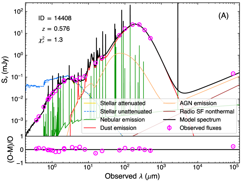
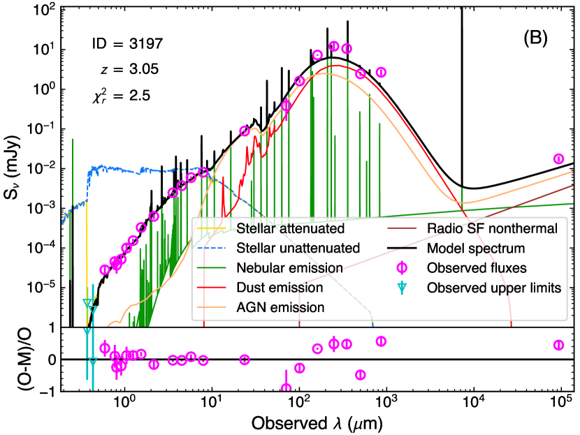
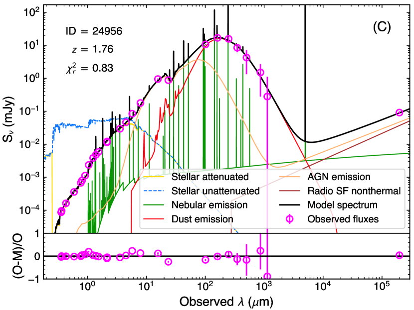
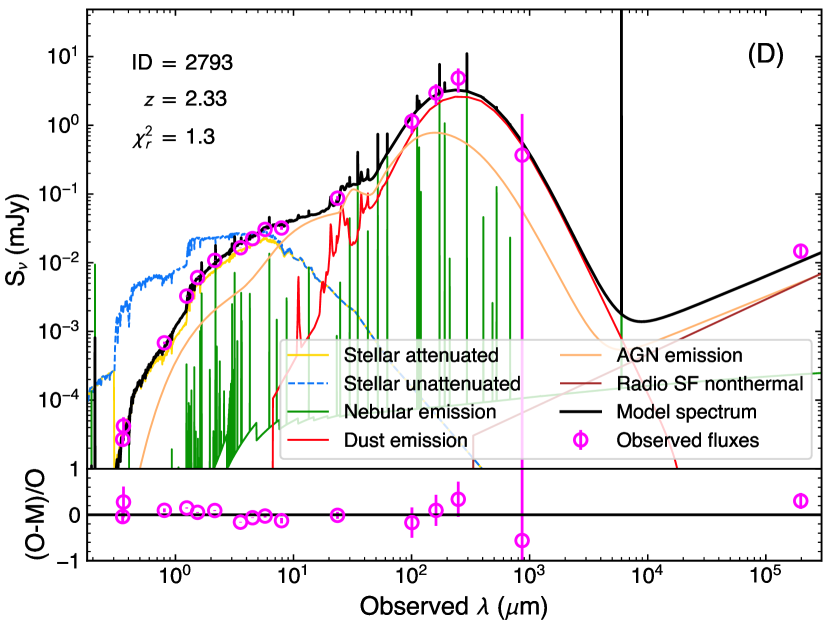
| \addstackgap[.5] Module | Parameter | Symbol | Values |
|---|---|---|---|
| \addstackgap[.5] Star formation history | Stellar -folding time | ( yr) | 50, 100, 250, 500, 1000, 2500, 5000, 10000 |
| Stellar age | ( yr) | 100, 250, 500, 1000, 2500, 5000, 10000 | |
| \addstackgap[.5] Single stellar population | Initial mass function | – | Chabrier (2003) |
| (Bruzual & Charlot 2003) | Metallicity | 0.02 | |
| \addstackgap[.5] Dust attenuation | Color excess of the nebular lines | (mag) | 0.005, 0.05, 0.1–0.7 (step 0.1), 0.9, 1.1, 1.3, 1.5 |
| (Calzetti et al. 2000) | |||
| \addstackgap[.5] Galactic dust emission | Slope in | 1.25, 1.5, 1.75, 2.0, 2.25, 2.5, 2.75 | |
| (Dale et al. 2014) | |||
| \addstackgap[.5] AGN (UV-to-IR) | AGN contribution to IR luminosity | 0.0, 0.01, 0.1, 0.3, 0.5, 0.7, 0.9, 0.99 | |
| Viewing angle | , | ||
| Polar-dust color excess | (mag) | 0.0, 0.2, 0.4 | |
| \addstackgap[.5] Radio | SF radio-IR correlation parameter | 2.58 | |
| Radio-loudness parameter | 0.0, 0.01, 0.1, 1, 10, 100, 1000, 10000 |
Appendix B Radio luminosity function in each field: GOODS-N, GOODS-S, and COSMOS/UltraVISTA fields
We obtain the radio luminosity function in each field following the same procedure described in Section 5. For both SFGs and radio-excess AGNs, RLFs in these three fields present generally consistent results (see detailed discussions in Section 5).
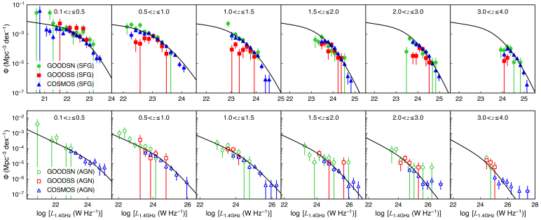
Appendix C Radio luminosity function for radio-excess AGN split into the subsets hosted by SFGs and QGs
We obtain the radio luminosity function for radio-excess AGN hosted by different populations (SFGs and QGs) following the same procedure described in Section 5. We found a similar evolution trend for radio-excess AGN hosted by different populations to that for low-excitation radio galaxies in Kondapally et al. (2022) (see detailed discussions in Section 5.3).
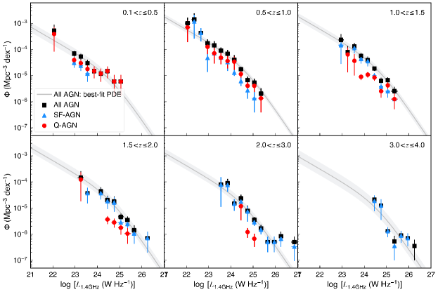
Appendix D Correct the classification purity for the radio-excess AGN
We use the cross point between the highest and the second highest gaussian components of distribution as the threshold to select radio-excess AGN (see details in Section 4.1). Radio-excess AGNs with around the selection threshold (corresponds to the in Fig. 3 and the vertical black dash-dotted lines in Fig. D.4) are partially contaminated by the SFGs. To correct the classification purity for radio-excess AGN, we follow Delvecchio et al. (2022) to define as the , where represents the best-fit gaussian model for the highest peak (see the highest dotted curves in Fig. D.4), and represents the best-fit model for the entire distribution (see the entire purple solid curves in Fig. D.4). At the threshold (see the black dash-dotted line in Fig. D.4), is usually below 50 for samples in the GOODS-S and COSMOS fields, while is around 100 for the GOODS-N field. It indicates that the Radio-excess AGN Sample in the GOODS-N have a nearly 100% AGN purity under the selection threshold used in this work. Therefore, we only make AGN purity corrections for the objects in the GOODS-S and COSMOS fields. Following Delvecchio et al. (2022), we use the threshold converted from the median IR luminosity in each redshift bin to make the purity corrections.
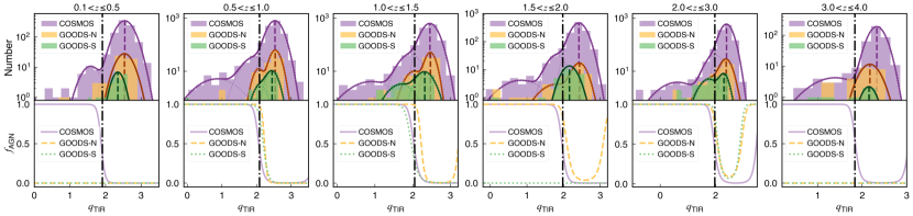
Appendix E Simple fits to the probability of hosting a radio-excess AGN in each redshift bin
As Equation 22 or 23 shows, at each fixed (or ), we assume a simple power-law relation for as a function of (or ). Then we apply fits to the data (see colored symbols in Fig. E.5 and Fig. E.6). The best-fit model in each (or ) bin is shown as the colored line in the left column of Fig. E.5 (or Fig. E.6). The best-fit parameters in each (or ) bin are shown as colored points in the right column of Fig. E.5 (or Fig. E.6). For more details about analysis and discussion, we refer readers to Section 6.3.3.
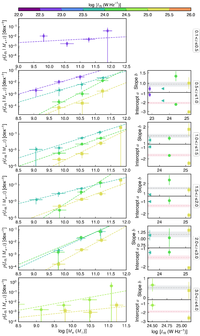
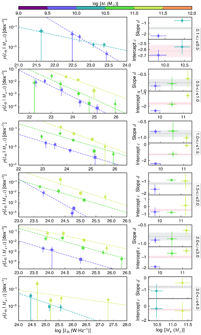
Appendix F The probability of hosting a radio-excess AGN in QGs and all the galaxies
Similar to Section 6.3 (mainly for SFGs), here we show the probability of hosting a radio-excess AGN in QGs and all the galaxies based on maximum-likelihood fitting over the entire redshift range.
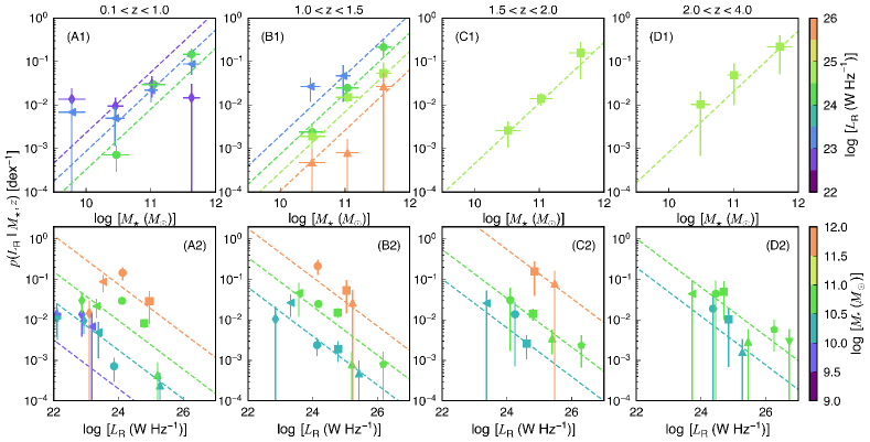
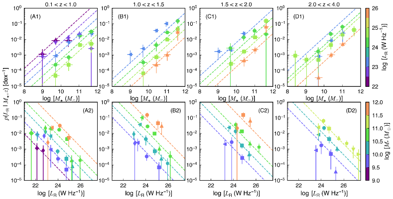
Appendix G The evolution of in SFGs considering the -dependent IRRC
In order to examine whether the -dependent IRRC will affect our results, we follow van der Vlugt et al. (2022) to select radio-excess AGNs with deviating more than from the -dependent IRRC of Delvecchio et al. (2021). To compare with the results shown in Section 6.3 (see the green region in Fig. G.9), we also use Equation 28 to recalculate the probability of SFGs hosting a radio-excess AGN (see the dark blue region in Fig. G.9). Fig. G.9 shows that using the -dependent IRRC (Delvecchio et al. 2021) does not alter the results in this work.
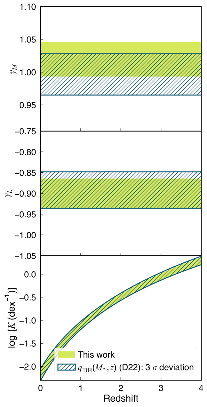
Appendix H Tables of radio luminosity functions for SFGs and radio-excess AGNs
| \addstackgap[.5] | ||||||||
|---|---|---|---|---|---|---|---|---|
| 4 | 3 | 15 | ||||||
| 12 | 14 | 42 | ||||||
| 9 | 52 | 162 | ||||||
| 27 | 134 | 281 | ||||||
| 48 | 208 | 292 | ||||||
| 45 | 329 | 214 | ||||||
| 82 | 373 | 140 | ||||||
| 124 | 296 | 67 | ||||||
| 132 | 193 | 42 | ||||||
| 125 | 111 | 8 | ||||||
| 111 | 45 | |||||||
| 77 | 29 | |||||||
| 39 | 7 | |||||||
| 34 | 4 | |||||||
| 9 | ||||||||
| 4 | ||||||||
| 4 | ||||||||
| 2 | 13 | 2 | ||||||
| 6 | 97 | 12 | ||||||
| 72 | 211 | 81 | ||||||
| 230 | 317 | 119 | ||||||
| 282 | 228 | 81 | ||||||
| 206 | 176 | 57 | ||||||
| 158 | 93 | 21 | ||||||
| 65 | 30 | 7 | ||||||
| 26 | 10 | |||||||
| 13 | 4 | |||||||
| 2 | ||||||||
| \addstackgap[.5] | ||||||||
|---|---|---|---|---|---|---|---|---|
| 3 | 3 | 3 | ||||||
| 13 | 4 | 3 | ||||||
| 27 | 6 | 33 | ||||||
| 23 | 21 | 88 | ||||||
| 18 | 58 | 71 | ||||||
| 11 | 89 | 44 | ||||||
| 6 | 67 | 16 | ||||||
| 4 | 51 | 16 | ||||||
| 5 | 26 | 6 | ||||||
| 10 | ||||||||
| 8 | ||||||||
| 3 | ||||||||
| 3 | 2 | 6 | ||||||
| 3 | 8 | 7 | ||||||
| 10 | 9 | 7 | ||||||
| 43 | 25 | 3 | ||||||
| 44 | 25 | 5 | ||||||
| 33 | 21 | 4 | ||||||
| 13 | 10 | 2 | ||||||
| 10 | 3 | |||||||
| 4 | 3 | |||||||
| 5 | ||||||||
| 3 | ||||||||