Regularity of sets of finite fractional perimeter and nonlocal minimal surfaces in metric measure spaces

Abstract.

In the setting of a doubling metric measure space $(X,d,\mu)$, we study regularity of sets whose characteristic functions belong to the Besov class $B^{s}_{1,1}(X)$. Following a result of Visintin in $\mathbb{R}^{n}$, we provide a sufficient condition for membership in $B^{s}_{1,1}(X)$ given in terms of the upper Minkowski codimension of the regularized boundary of the set. We also show that if the characteristic function of a set belongs to $B^{s}_{1,1}(X)$, then its measure theoretic boundary has codimension $s$ Hausdorff measure zero. To the best of our knowledge, this result is new even in the Euclidean setting. By studying certain fat Cantor sets, we provide examples illustrating that the converses of these results do not hold in general. In the doubling metric measure space setting, we then consider minimizers of the nonlocal perimeter functional $\mathcal{J}_{\Omega}^{s}$, extending the definition introduced by Caffarelli, Roquejoffre, and Savin in $\mathbb{R}^{n}$, and prove existence, uniform density, and porosity results for minimizers.

1. Introduction

In the setting of a doubling metric measure space $(X,d,\mu)$, we consider measurable sets $E\subset X$ for which the following Besov energy is finite for some fractional parameter $0<s<1$:

$$\|\chi_{E}\|_{B^{s}_{1,1}(X)}=\int_{X}\int_{X}\frac{|\chi_{E}(x)-\chi_{E}(y)|}{d(x,y)^{s}\mu(B(x,d(x,y))}d\mu(y)d\mu(x).$$

Specifically, we study regularity properties of these sets of finite $s$-perimeter and minimizers of the $s$-perimeter functional with respect to a given bounded domain $\Omega$.

In the celebrated work of Bourgain, Brezis, and Mironescu [11], it was shown that for $p>1$, functions in $W^{1,p}(\mathbb{R}^{n})$ are characterized by the limiting behavior of the Besov $B^{s}_{p,p}$-energy, under suitable rescaling, as $s\to 1^{-}$. It was then shown by Dávila [16] that the same characterization holds for functions in $BV(\mathbb{R}^{n})$ when $p=1$. That is, given a measurable set $E\subset\mathbb{R}^{n}$,

$$\lim_{s\to 1^{-}}(1-s)\|\chi_{E}\|_{B^{s}_{1,1}(\mathbb{R}^{n})}=C_{n}P(E,\mathbb{R}^{n}),$$

where $P(E,\mathbb{R}^{n})$ is the perimeter of $E$, given by the BV energy of $\chi_{E}$, and $C_{n}$ is a dimensional constant. More recently, Di Marino and Squassina [17] proved analogous results in the setting of a complete, doubling metric measure space supporting a $(1,p)$-Poincaré inequality. When $p=1$, they showed that

$$P(E,X)\lesssim\liminf_{s\to 1^{-}}(1-s)\|\chi_{E}\|_{B^{s}_{1,1}(X)}\leq\limsup_{s\to 1^{-}}(1-s)\|\chi_{E}\|_{B^{s}_{1,1}(X)}\lesssim P(E,X).$$

Hence, in both Euclidean and metric settings, sets of finite perimeter are characterized by the limiting behavior of their $s$-perimeters. For more on characterization of Sobolev and BV functions in the metric setting by nonlocal functionals, see [32, 46, 47, 44].

Federer’s characterization [28] states that $E\subset\mathbb{R}^{n}$ is a set of finite perimeter if and only if $\mathcal{H}^{n-1}(\partial^{*}E)<\infty$, where $\partial^{*}E$ is the measure theoretic boundary of $E$, see Section 2.2. In the setting of a complete, doubling metric measure space supporting a $(1,1)$-Poincaré inequality, the “only if” direction was proved by Ambrosio [3], and more recently the “if” direction was shown by Lahti [45]. Here the codimension 1 Hausdorff measure $\mathcal{H}^{-1}$ was used as a replacement for $\mathcal{H}^{n-1}$, see Section 2.2. In fact, it was shown in [3, 43] that this characterization holds in this setting with $\partial^{*}E$ replaced with a smaller subset of the boundary, namely points where $E$ and its complement have lower density bounded below by a constant which depends only on the doubling and Poincaré constants, see Section 2.4. As sets of finite perimeter are characterized both by this boundary regularity and the limiting behavior of their $s$-perimeters, we first consider in this paper the relationship between the $s$-perimeter of a set and codimension $s$ measurements of its boundary.

The von Koch snowflake domain $K\subset\mathbb{R}^{2}$ shows that the “if” direction of Federer’s characterization does not hold in the fractional case. Indeed, it was shown in [48] that $\chi_{K}\in B^{s}_{1,1}(\mathbb{R}^{2})$ if and only if $s\in(0,2-\log 4/\log 3)$. Since $\partial K=\partial^{*}K$ and $\mathcal{H}^{\log 4/\log 3}(\partial K)<\infty$ (see [27] for example), we see that $\mathcal{H}^{n-s}(\partial^{*}E)<\infty$ does not imply that $E$ is a set of finite $s$-perimeter in general. However, considering the upper Minkowski content rather than the Hausdorff measure provides a sufficient condition for finiteness of the $s$-perimeter. In [54], the following fractional codimension was introduced by Visintin for bounded sets $E\subset\mathbb{R}^{n}$,

$$\operatorname{codim}_{F}(E)=\sup\{0<s<1:\chi_{E}\in B^{s}_{1,1}(\mathbb{R}^{n})\},$$

and it was shown that this codimension is bounded below by the upper Minkowski codimension of the regularized boundary $\partial^{+}E$ of $E$. The regularized boundary contains the measure theoretic boundary, and any set can be modified on a set of measure zero so that its topological boundary coincides with its regularized boundary, see Lemma 2.7. See Section 2.2 for the precise definitions of the regularized boundary and Minkowski contents and codimensions. We first generalize this result from [54] to the doubling metric measure space setting. For the following and subsequent result, we denote our ambient metric measure space by $(Z,d,\nu)$, rather than $(X,d,\mu)$, in order to avoid confusion with the hyperbolic filling, used in the same section.

Theorem 1.1.

Let $(Z,d,\nu)$ be a metric measure space satsifying the LLC-1 condition, with $\nu$ a doubling measure. Let $E\subset Z$ be a bounded measurable set, and suppose that there exists $t>0$ such that $\overline{\mathcal{M}}^{-t}(\partial^{+}E)<\infty$. Then $\chi_{E}\in B^{s}_{1,1}(Z)$ for all $0<s<t$.

Here, $\overline{\mathcal{M}}^{-t}$ is the codimension $t$ upper Minkowski content, defined in Section 2.2, and the LLC-1 condition, defined in Section 2.1, is a connectedness condition on $Z$. In Example 3.6, we show that the conclusion to Theorem 1.1 may fail if $Z$ does not satisfy this condition. Furthermore, by constructing certain fat Cantor sets, we show in Example 4.10 that the converse to Theorem 1.1 does not hold in general. In fact, we provide an example of a set $E\in B^{s}_{1,1}(Z)$ for which $\partial^{*}E\subsetneq\partial^{+}E$ and $\underline{\mathcal{M}}^{-t}(\partial^{*}E)=\infty$ for all $0<t<1$. Thus, the converse does not hold even with the weaker conclusion of $\underline{\mathcal{M}}^{-t}(\partial^{*}E)<\infty$. Here $\underline{\mathcal{M}}^{-t}$ is the codimension $t$ lower Minkowski content, see Section 2.2. For related results in the setting of strongly local Dirichlet metric spaces with sub-Gaussian heat kernel estimates, see [2, Section 5.3].

We then study necessary conditions for finiteness of the $s$-perimeter in the metric setting, and obtain the following result:

Theorem 1.2.

Let $(Z,d,\nu)$ be a compact metric measure space with $\nu$ a doubling measure, and let $0<s<1$. If $E\subset Z$ is such that $\chi_{E}\in B^{s}_{1,1}(Z)$, then $\mathcal{H}^{-s}(\partial^{*}E)=0$.

Here, $\mathcal{H}^{-s}$ is the codimension $s$ Hausdorff measure, see Section 2.2. To the best of our knowledge, this result is new even in the Euclidean setting. To prove this result, we utilize recent developments from analysis in metric spaces pertaining to the hyperbolic filling of a compact, doubling metric measure space. In [8], it was shown that any compact, doubling metric measure space $(Z,d,\nu)$ can be realized as the boundary of a uniform metric measure space $X$ which is doubling and supports a $(1,1)$-Poincaré inequality. Furthermore, bounded trace and extension operators exist between the Besov spaces $B^{s}_{p,p}(Z)$ and the Newton-Sobolev spaces $N^{1,p}(X)$. See Theorem 2.15 and Section 2.5 below for an outline of the construction of the hyperbolic filling. To study the measure theoretic properties of $E\subset Z$, we consider the Newton-Sobolev extension of $\chi_{E}$ to the hyperbolic filling of $Z$. There, the validity of a $(1,1)$-Poincaré inequality provides us with useful potential theoretic tools with which to study $\partial^{*}E$. As with Theorem 1.1, we also construct certain fat Cantor sets in Example 4.9 which illustrate that the converse of Theorem 1.2 does not hold in general. This construction also shows that Theorem 1.2 is sharp in the sense that we cannot replace $\mathcal{H}^{-s}(\partial^{*}E)=0$ with $\mathcal{H}^{-t}(\partial^{+}E)<\infty$. Indeed, we show in Example 4.8 that there exists a fat Cantor set $C_{a}$ such that $\chi_{C_{a}}\in B^{s}_{1,1}([0,1])$, but $\mathcal{H}^{-t}(\partial^{+}C_{a})=\infty$ for all $0<t<1$.

By combining Theorem 1.1 and Theorem 1.2, we obtain the following corollary, which generalizes the result from [54] to the metric setting and provides a new upper bound in terms of the Hausdorff codimension. See Section 2.2 and 2.6 for the precise definitions.

Corollary 1.3.

Let $(Z,d,\nu)$ be a compact metric measure space satisfying the LLC-1 condition, with $\nu$ a doubling measure. Let $E\subset Z$ be measurable. Then,

(1.4) $$\overline{\operatorname{codim}}_{\mathcal{M}}(\partial^{+}E)\leq\operatorname{codim}_{F}(E)\leq\operatorname{codim}_{\mathcal{H}}(\partial^{*}E).$$

In [48], it was shown that (1.4) holds with equality when $E\subset\mathbb{R}^{2}$ is the von Koch snowflake domain. In Example 4.11, we show that these inequalities may be strict, again by constructing a certain fat Cantor set.

In the second half of this paper, we consider a doubling metric measure space $(X,d,\mu)$, and fix a bounded domain $\Omega\subset X$ and $0<s<1$. We then study minimizers of the $\mathcal{J}_{\Omega}^{s}$ functional, defined here in Section 2.6, as originally introduced in $\mathbb{R}^{n}$ by Caffarelli, Roquejoffre, and Savin [15]. Related to problems arising in phase transitions, motion by mean curvature, and front propogation, see for example [1, 38, 39, 40, 53], this functional measures the interaction between a set and its complement given by the $B^{s}_{1,1}$-seminorm, but excludes the interaction occurring in the complement of $\Omega$. In [15], existence and regularity of minimizers, referred to there as nonlocal minimal surfaces, were studied for Lipschitz domains $\Omega\subset\mathbb{R}^{n}$. In particular, it was shown that if $E\subset\mathbb{R}^{n}$ is a minimizer, then $\partial E\cap\Omega$ is a $C^{1,\alpha}$-hypersurface around each of its points, outside of an $n-2$ dimensional set. Since their introduction in [15], nonlocal minimal surfaces have been studied at great length and remain a subject of active research in the Euclidean setting, see for example [14, 21, 20, 29, 50] and references therein. Of particular interest are asymptotic results as the nonlocal parameter $s$ converges to either $0$ or $1$ and the “stickiness” phenomenon which is exhibited by nonlocal minimal surfaces, see for example [23, 13, 12, 22, 19]. For $\Gamma$-convergence results regarding the $\mathcal{J}_{\Omega}^{s}$ functional, see [5].

We consider this problem in the doubling metric measure space setting, and first prove an existence result via the direct method of calculus of variations in Theorem 5.9. To do so, we first prove a compactness result in Theorem 5.2 by adapting the proof of [18, Theorem 7.1] to the metric setting. We then obtain the following uniform density result, which was established in [15, Theorem 4.1] in the Euclidean setting:

Theorem 1.5.

Let $(X,d,\mu)$ be a connected doubling metric measure space, let $\Omega\subset X$ a bounded domain and let $0<s<1$. Then there exists a constant $\gamma_{0}>0$, such that if $E\subset X$ is a minimizer of $\mathcal{J}_{\Omega}^{s}$, then after possibly modifying $E$ on a set of measure zero, it follows that for all $x_{0}\in\partial E\cap\Omega$ and $R_{0}>0$ such that $B(x_{0},2R_{0})\subset\Omega$, we have

(1.6) $$\frac{\mu(B(x_{0},R_{0})\cap E)}{\mu(B(x_{0},R_{0}))}\geq\gamma_{0}\quad\text{and}\quad\frac{\mu(B(x_{0},R_{0})\setminus E)}{\mu(B(x_{0},R_{0}))}\geq\gamma_{0}.$$

Here, the constant $\gamma_{0}$ depends only on $s$ and the doubling constant of $\mu$.

The connectedness assumption on $X$ can be relaxed, see Remark 6.4. Our proof is inspired by the arguments of [42, Theorem 4.2], where an analogous uniform density result was obtained for minimizers of the (local) perimeter functional, in the setting of a doubling metric measure space supporting a $(1,1)$-Poincaré inequality. There, the result is obtained via the De Giorgi method, where the Poincaré inequality plays a crucial role. Since we are dealing with the fractional case, we do not require the validity of a Poincaré inequality, instead utilizing a fractional Poincaré inequality [24, Theorem 3.4], which is valid without additional assumptions on $X$.

As a consequence of Theorem 1.5, we obtain the following porosity results for minimizers. In the Euclidean setting, this was established in [15, Corollary 4.3].

Theorem 1.7.

Let $(X,d,\mu)$ be a doubling metric measure space satisfying the LLC-1 condition, let $\Omega\subset X$ be a bounded domain, and let $0<s<1$. Then there exists a constant $C\geq 1$ such that if $E$ is a minimizer of $\mathcal{J}^{s}_{\Omega}$, then after possibly modifying $E$ on a set of measure zero, it follows that for all $x_{0}\in\partial E\cap\Omega$ and $R_{0}>0$ such that $B(x_{0},2R_{0})\subset\Omega,$ there exist $y,z\in B(x_{0},R_{0})$ such that

(1.8) $$B(y,R_{0}/C)\subset E\cap\Omega\text{ and }B(z,R_{0}/C)\subset\Omega\setminus E.$$

The constant $C$ depends only on $s$, the doubling constant of $\mu$, and the constant $C_{L}$ from the LLC-1 condition.

We point out that Theorem 1.5 follows also from Theorem 1.7. However, to prove Theorem 1.7, we use the uniform density result of Theorem 1.5, and so we prove it independently. As in Theorem 1.5, our proof is inspired by the arguments used to obtain the corresponding porosity results for minimizers of the local perimeter functional in [42, Theorem 5.2]. As before, however, the argument there utilizes the $(1,1)$-Poincaré inequality, which we do not assume in our case. As a corollary to Theorem 1.7, we see that if $E$ is a minimizer of $\mathcal{J}_{\Omega}^{s}$ with $\chi_{E}\in B^{s}_{1,1}(X)$, then $\partial E\cap\Omega\subset\partial^{*}E$, and so by Theorem 1.2, we have that $\mathcal{H}^{-s}(\partial E\cap\Omega)=0$, see Corollary 6.10.

The structure of the paper is as follows: in Section 2 we introduce the necessary definitions and background notions, and in Section 3, we prove Theorems 1.1 and 1.2. In Section 4, we establish examples illustrating sharpness of the results of Section 3 and that the converses of these results do not hold. In Section 5, we prove existence results for minimizers of $\mathcal{J}_{\Omega}^{s}$, and in Section 6, we prove Theorems 1.5 and 1.7.

2. Preliminaries

2.1. Doubling and connectedness properties

Given a metric measure space $(X,d,\mu)$, we say that the measure $\mu$ is doubling if there exists a constant $C_{\mu}\geq 1$ such that

$$0<\mu(B(x,2r))\leq C_{\mu}\mu(B(x,r))<\infty$$

for all $x\in X$ and $r>0$. By iterating this condition, there are constants $C_{Q}\geq 1$ and $Q\geq 1$, depending only on $C_{\mu}$, such that

(2.1) $$\frac{\mu(B(y,r))}{\mu(B(x,R))}\geq C_{Q}^{-1}\left(\frac{r}{R}\right)^{Q}$$

for all $x\in X$, $0<r\leq R$, and $y\in B(x,R)$. We say that $\mu$ is reverse doubling if the opposite relationship holds, that is, if there exist constants $C_{\sigma}\geq 1$ and $\sigma>0$ such that for all $x\in X$, $0<r\leq R$, and $y\in B(x,R)$, we have

(2.2) $$\frac{\mu(B(y,r))}{\mu(B(x,R))}\leq C_{\sigma}\left(\frac{r}{R}\right)^{\sigma}.$$

The reverse doubling condition holds if $\mu$ is doubling and $X$ is connected, see for example [7, Corollary 3.8], with constants $\sigma$ and $C_{\sigma}$ depending only on $C_{\mu}$. Throughout this paper, we let $C$ denote a constant which depends, unless otherewise stated, only on the structural constants, such as the doubling constant for example. Its specific value is not of interest, and may vary with each occurrence, even within the same line. Given quantities $A$ and $B$, we use the notation $A\simeq B$ to mean that there exists such a constant $C\geq 1$ such that $C^{-1}A\leq B\leq CA$. Likewise, we use $\lesssim$ and $\gtrsim$ if the left and right inequalities hold, respectively.

As a consequence of the doubling property, we have the following covering lemma, see for example [33, Appendix B7] and [37, Section 3.3]:

Lemma 2.3.

Let $(X,d,\mu)$ be a doubling metric measure space. For any $\varepsilon>0$, there exists a countable cover $\{B_{i}\}_{i}$ of $X$ by balls with $\operatorname{rad}(B_{i})=\varepsilon$ such that the collection $\{\frac{1}{5}B_{i}\}_{i}$ is pairwise disjoint. Moreover, $\{B_{i}\}_{i}$ has bounded overlap in the sense that for all $K>0$, there exists a constant $C$ depending only on $K$ and $C_{\mu}$ such that

$$\sum_{i}\chi_{KB_{i}}\leq C.$$

Here and throughout the paper, we denote by $\operatorname{rad}(B)$ the radius of a ball $B$. We associate to this cover the following Lipschitz partition of unity, see [33, Appendix B7]:

Lemma 2.4.

Let $(X,d,\mu)$ be a doubling metric measure space, and let $\varepsilon>0$ and $\{B_{i}\}_{i}$ be as in Lemma 2.3. Then there exists a constant $C\geq 1$ such that for each $i$, there exists a $C/\varepsilon$-Lipschitz function $\varphi_{i}^{\varepsilon}$ satisfying $0\leq\varphi_{i}^{\varepsilon}\leq 1$, $\operatorname{supt}(\varphi_{i}^{\varepsilon})\subset 2B_{i}$, and $\sum_{i}\varphi_{i}^{\varepsilon}\equiv 1$. Here the constant $C$ depends only on $C_{\mu}$.

These preceding lemmas will be used in Section 5 to construct a discrete convolution of a locally integrable function $f$:

$$f_{\varepsilon}=\sum_{i}f_{B_{i}}\varphi_{i}^{\varepsilon}.$$

Here and throughout the paper, we denote

$$f_{B}=\fint_{B}f\,d\mu=\frac{1}{\mu(B)}\int_{B}f\,d\mu.$$

At times, we will assume that $X$ satisfies the following connectedness property:

Definition 2.5.

We say that a metric space $(X,d)$ is linearly locally connected (LLC) if there exists a constant $C_{L}\geq 1$ such that for all $x\in X$ and $r>0$, the following conditions hold:

1. Any two points in $B(x,r)$ can be joined by a connected set in $B(x,C_{L}r)$.

2. Any two points in $X\setminus\overline{B}(x,r)$ can be joined by a connected set in $X\setminus\overline{B}(x,r/C_{L}).$

We say that $X$ is LLC-1 if the first condition holds and LLC-2 if the second condition holds.

2.2. Measure theoretic boundary, Minkowski content, and Hausdorff measure

Definition 2.6.

Let $E\subset X$. We define the regularized boundary of $E$, denoted $\partial^{+}E$, to be the collection of points $x\in X$ such that

$$\mu(B(x,r)\cap E)>0\quad\text{and}\quad\mu(B(x,r)\setminus E)>0$$

for all $r>0$. We define the measure theoretic boundary of $E$, denoted $\partial^{*}E$, to be collection of points $x\in X$ such that

$$\limsup_{r\to 0^{+}}\frac{\mu(B(x,r)\cap E)}{\mu(B(x,r))}>0\quad\text{and}\quad\limsup_{r\to 0^{+}}\frac{\mu(B(x,r)\setminus E)}{\mu(B(x,r))}>0.$$

We note that $\partial^{*}E\subset\partial^{+}E\subset\partial E$, with $\partial E$ being the topological boundary of $E$.

With the following lemma, we show that any measureable set can be modified on a set of measure zero so that its regularized boundary coincides with its topological boundary.

Lemma 2.7.

If $E\subset X$ is measurable, then there exists $\widetilde{E}\subset X$ such that $\mu(E\Delta\widetilde{E})=0$ and $\partial^{+}E=\partial^{+}\widetilde{E}=\partial\widetilde{E}$.

Proof.

We define the following sets,

$$E_{-}:=\{x\in E:\exists r>0\text{ s.t. }\mu(B(x,r)\cap E)=0\}$$

$$E_{+}:=\{x\in X\setminus E:\exists r>0\text{ s.t. }\mu(B(x,r)\setminus E)=0\},$$

and note that $E_{-}\cup E_{+}\subset\partial E$. Let $\widetilde{E}=(E\setminus E_{-})\cup E_{+}$. It follows that $\mu(E_{-})=0=\mu(E_{+})$ by the Lebesgue differentiation theorem, and so $\mu(E\Delta\widetilde{E})=0$. As such, we have that $\partial^{+}E=\partial^{+}\widetilde{E}$ by the definition of the regularized boundary. Since $\partial^{+}\widetilde{E}\subset\partial\widetilde{E}$, it remains to show the opposite inclusion.

Let $z\in\partial\widetilde{E}$, and let $r>0$. Then there exists $x\in B(z,r/2)\cap\widetilde{E}$. If $x\in E\setminus E_{-}$, then for all $\rho>0$, we have that

$$\mu(B(x,\rho)\cap\widetilde{E})=\mu(B(x,\rho)\cap E)>0,$$

since $\mu(E\Delta\widetilde{E})=0$. Hence, $\mu(B(z,r)\cap\widetilde{E})\geq\mu(B(x,r/2)\cap\widetilde{E})>0$. If $x\in E_{+}$, then there exists $r_{x}>0$ such that $\mu(B(x,r_{x})\setminus\widetilde{E})=\mu(B(x,r_{x})\setminus E)=0$, and so we necessarily have that

$$\mu(B(z,r)\cap\widetilde{E})>0.$$

Hence, for all $r>0$, we have that $\mu(B(z,r)\cap\widetilde{E})>0$.

Likewise, since $z\in\partial\widetilde{E}$, there exists $y\in B(z,r/2)\setminus\widetilde{E}$. If $y\in E$, then we have that $y\in E_{-}$, in which case there exists $r_{y}>0$ such that $\mu(B(y,r_{y})\cap\widetilde{E})=\mu(B(y,r_{y})\cap E)=0$. Then necessarily we have that $\mu(B(z,r)\setminus\widetilde{E})>0$. If $y\in X\setminus E$, then $y\in X\setminus E_{+}$, and so

$$\mu(B(z,r)\setminus\widetilde{E})\geq\mu(B(y,r/2)\setminus\widetilde{E})=\mu(B(y,r/2)\setminus E)>0.$$

Therefore, for all $r>0$, we have $\mu(B(z,r)\setminus\widetilde{E})>0$, and so $z\in\partial^{+}\widetilde{E}$. ∎

Definition 2.8.

Let $E\subset X$, let $t>0$, and let $r>0$. We define the codimension $t$ Minkowski $r$-content of $E$ by

$$\mathcal{M}^{-t}_{r}(E):=\inf\left\{r^{-t}\sum_{i}\mu(B(x_{i},r)):E\subset\bigcup_{i}B(x_{i},r),\,x_{i}\in E\right\},$$

and we define the codimension $t$ upper and lower Minkowski contents of $E$, respectively, by

$$\overline{\mathcal{M}}^{-t}(E)=\limsup_{r\to 0^{+}}\mathcal{M}^{-t}_{r}(E)\quad\text{ and }\quad\underline{\mathcal{M}}^{-t}(E)=\liminf_{r\to 0^{+}}\mathcal{M}^{-t}_{r}(E).$$

The upper and lower Minkowski codimensions of $E$ are defined, respectively, by

$$\overline{\operatorname{codim}}_{\mathcal{M}}(E)=\sup\{t>0:\overline{\mathcal{M}}^{-t}(E)<\infty\}\quad\text{and}\quad\underline{\operatorname{codim}}_{\mathcal{M}}(E)=\sup\{t>0:\underline{\mathcal{M}}^{-t}(E)<\infty\}.$$

Note that $\underline{\mathcal{M}}^{-t}(E)\leq\overline{\mathcal{M}}^{-t}(E)$, and so $\overline{\operatorname{codim}}_{\mathcal{M}}(E)\leq\underline{\operatorname{codim}}_{\mathcal{M}}(E)$. We define the codimension $t$ Hausdorff $r$-content of $E$ to be

$$\mathcal{H}^{-t}_{r}(E):=\inf\left\{\sum_{i}\frac{\mu(B_{i})}{\operatorname{rad}(B_{i})^{t}}:E\subset\bigcup_{i}B_{i},\,\operatorname{rad}(B_{i})\leq r\right\},$$

and likewise, we define the codimension $t$ Hausdorff measure of $E$ by

$$\mathcal{H}^{-t}(E)=\lim_{r\to 0^{+}}\mathcal{H}^{-t}_{r}(E).$$

The Hausdorff codimension of $E$ is defined by

$$\operatorname{codim}_{\mathcal{H}}(E)=\sup\{t>0:\mathcal{H}^{-t}(E)<\infty\}.$$

At times we will be considering Hausdorff contents and measures with respect to different references measures. In these cases we will include the reference measure as a subscript in the notation ($\mathcal{H}^{-t}_{\mu,r}(E)$ and $\mathcal{H}^{-t}_{\mu}(E)$, for example). However, if the reference measure is clear from context, we will drop the reference to simplify the notation.

2.3. Newton-Sobolev, BV, and Besov classes

Let $1\leq p<\infty$. Given a family $\Gamma$ of non-constant, compact, rectifiable curves, we define the $p$-modulus of $\Gamma$ by

$$\operatorname{Mod}_{p}(\Gamma)=\inf_{\rho}\int_{X}\rho^{p}d\mu,$$

where the infimum is taken over all Borel functions $\rho:X\to[0,\infty]$ such that $\int_{\gamma}\rho\,ds\geq 1$ for all $\gamma\in\Gamma$. We refer the interested reader to [37] for more on modulus of curve families. Given a function $u:X\to\overline{\mathbb{R}}$, we say that a Borel function $g:X\to[0,\infty]$ is an upper gradient of $u$ if the following holds for all non-constant, compact, rectifiable curves $\gamma:[a,b]\to X$:

$$|u(x)-u(y)|\leq\int_{\gamma}g\,ds,$$

whenever $u(x)$ and $u(y)$ are both finite, and $\int_{\gamma}g\,ds=\infty$ otherwise. Here $x$ and $y$ denote the endpoints of $\gamma$. Upper gradients were first defined in [36]. We say that $g$ is a $p$-weak upper gradient of $u$ if the $p$-modulus of the family of curves where the above inequality fails is zero.

For $1\leq p<\infty$, we define $\widetilde{N}^{1,p}(X)$ to be the class of all functions in $L^{p}(X)$ which have an upper gradient belonging to $L^{p}(X)$, and we define

$$\|u\|_{\widetilde{N}^{1,p}(X)}=\|u\|_{L^{p}(X)}+\inf_{g}\|g\|_{L^{p}(X)},$$

where the infimum is taken over all upper gradients $g$ of $u$. We then define an equivalence relation in $\widetilde{N}^{1,p}(X)$ by $u\sim v$ if and only if $\|u-v\|_{\widetilde{N}^{1,p}(X)}=0$. The Newton-Sobolev space $N^{1,p}(X)$ is then defined to be $\widetilde{N}^{1,p}(X)/\sim$, equipped with the norm $\|\cdot\|_{N^{1,p}(X)}:=\|\cdot\|_{\widetilde{N}^{1,p}(X)}$. One can similarly define $N^{1,p}(\Omega)$ for any open set $\Omega\subset X$. Each $u\in N^{1,p}(X)$ has a minimal $p$-weak upper gradient, denoted $g_{u}$, which is unique up to sets of measure zero, see for example [37, Chapter 6]. For more on $p$-modulus, upper gradients, and the Newton-Sobolev class, see [52, 7, 35, 37].

Following Miranda Jr. [51] we define the total variation of a function $u\in L^{1}_{\text{loc}}(X)$, by

$$\|Du\|(X):=\inf\left\{\liminf_{i\to\infty}\int_{X}g_{u_{i}}\,d\mu:N^{1,1}_{\text{loc}}(X)\ni u_{i}\to u\text{ in }L^{1}_{\text{loc}}(X)\right\},$$

where $g_{u_{i}}$ is an upper gradient of $u_{i}$. For $u\in L^{1}(X)$, we say that $u\in BV(X)$, that is, $u$ is of bounded variation, if $\|Du\|(X)<\infty$. Similarly, we can define $\|Du\|(\Omega)$ and $BV(\Omega)$ for open sets $\Omega\subset X$. For an arbitrary set $A\subset X$, we then set

$$\|Du\|(A):=\inf\{\|Du\|(\Omega):A\subset\Omega,\,\Omega\text{ open}\}.$$

In [51], it was shown that $\|Du\|(\cdot)$ is a finite Radon measure on $X$ when $u\in BV(X)$. For a measurable set $E\subset X$, we say that $E$ is a set of finite perimeter if $\|D\chi_{E}\|(X)<\infty$, and we denote the perimeter of $E$ in $\Omega$ by

$$P(E,\Omega):=\|D\chi_{E}\|(\Omega).$$

For more on BV functions in the Euclidean and metric settings, see [26, 4, 6, 3].

For $0<s<1$ and $1\leq p<\infty$, we define the Besov energy of a function $u\in L^{1}_{\text{loc}}(X)$ by

$$\|u\|^{p}_{B^{s}_{p,p}(X)}:=\int_{X}\int_{X}\frac{|u(y)-u(x)|^{p}}{d(x,y)^{sp}\mu(B(x,d(x,y)))}d\mu(y)d\mu(x).$$

We then define the Besov space $B^{s}_{p,p}(X)$ to be the set of all functions $u\in L^{p}(X)$ for which this energy is finite. In $\mathbb{R}^{n}$, the space $B^{s}_{p,p}(\mathbb{R}^{n})$ corresponds to the fractional Sobolev space $W^{s,p}(\mathbb{R}^{n})$. In [31], it was shown that in doubling metric measure spaces supporting a $(1,p)$-Poincaré inequality (see below), $B^{\alpha}_{p,p}(X)$ coincides with the real interpolation space $(L^{p}(X),KS^{1,p}(X))_{\alpha,p}$, where $KS^{1,p}(X)$ is the Korevaar-Schoen Sobolev space.

2.4. Poincaré inequalities and consequences

Let $1\leq p<\infty$. We say that $(X,d,\mu)$ supports a $(1,p)$-Poincaré inequality if there exist constants $C\geq 1$ and $\lambda\geq 1$ such that

$$\fint_{B}|u-u_{B}|d\mu\leq C\operatorname{rad}(B)\left(\fint_{\lambda B}g^{p}\,d\mu\right)^{1/p}$$

for all balls $B\subset X$ and function-upper gradient pairs $(u,g)$. If $X$ is a length space supporting a $(1,p)$-Poincaré inequality, then we may take $\lambda=1$ [34]. If $u$ is locally integrable and possesses a $p$-integrable $p$-weak upper gradient in $X$, then the Poincaré inequality above holds with $g_{u}$, the minimal $p$-weak upper gradient of $u$, on the right hand side, see [37, Proposition 8.1.3].

When $(X,d,\mu)$ is a complete, doubling metric measure space supporting a $(1,1)$-Poincaré inequality, Federer’s characterization of sets of finite perimeter holds. That is, $E\subset X$ is such that $P(E,X)<\infty$ if and only if $\mathcal{H}^{-1}(\partial^{*}E)<\infty$ [3, 45]. In fact, it was shown by Ambrosio [3] (who proved the “only if” direction) and Lahti [43] (who proved the “if” direction), that there exists $\gamma>0$, depending only on the doubling and Poincaré constants, such that $P(E,X)<\infty$ if and only if $\mathcal{H}^{-1}(\Sigma_{\gamma}E)<\infty$. Here, $\Sigma_{\gamma}E$ is the set of all $x\in X$ such that

$$\liminf_{r\to 0^{+}}\frac{\mu(B(x,r)\cap E)}{\mu(B(x,r))}\geq\gamma\quad\text{and}\quad\liminf_{r\to 0^{+}}\frac{\mu(B(x,r)\setminus E)}{\mu(B(x,r))}\geq\gamma.$$

Let $1\leq p,q<\infty$ and let $0<s<1$. We say that $X$ supports an $(s,q,p,p)$-Poincaré inequality if there exist constants $C\geq 1$ and $\lambda\geq 1$ such that

$$\left(\fint_{B}|u-u_{B}|^{q}d\mu\right)^{1/q}\leq C\operatorname{rad}(B)^{s}\left(\fint_{\lambda B}\int_{\lambda B}\frac{|u(y)-u(x)|^{p}}{d(x,y)^{sp}\mu(B(x,d(x,y)))}d\mu(y)d\mu(x)\right)^{1/p}$$

for all $u\in L^{1}_{\text{loc}}(X)$ and balls $B\subset X$.

The validity of a $(1,p)$-Poincaré inequality implies a number of strong geometric properties of $X$, and as a result, it is often assumed as a standing assumption on $X$. Under mild assumptions on $X$ however, the fractional $(s,q,p,p)$-Poincaré inequality always holds:

Lemma 2.9.

[24, Lemma 2.2] Let $(X,d,\mu)$ be doubling. Let $0<s<1$ and let $1\leq p,q<\infty$ be such that $q\leq p$. Then $X$ supports an $(s,q,p,p)$-Poincaré inequality, with $\lambda=1$ and constant $C$ depending only on the $C_{\mu}$, $s$, $q$, and $p$.

If we additionally assume that $\mu$ is reverse doubling, then the exponent on the left-hand side can be improved as follows:

Theorem 2.10.

[24, Theorem 3.4] Let $\mu$ be reverse doubling. Let $0<s<1$ and $1\leq p<\infty$ be such that $sp<Q$, where $Q\geq 1$ is as in (2.2), and let $p^{*}=Qp/(Q-sp)$. Then $X$ supports an $(s,p^{*},p,p)$-Poincaré inequality with $\lambda=2$ and the constant $C$ depending only on $C_{\mu}$, $s$, $p$, and the constants from (2.1) and (2.2).

By applying this result to the case $p=1$, we obtain the following lemma, the proof of which follows mutatis mutandis from [42, Lemma 2.2]. We include the proof for the reader’s convenience.

Lemma 2.11.

Let $\mu$ be reverse doubling, and let $0<s<1$, and let $Q\geq 1$ be as in (2.1). There exists $C\geq 1$ such that if $u\in L^{1}_{\text{loc}}(X)$ and a ball $B\subset X$ are such that

(2.12) $$\frac{\mu(\{|u|>0\}\cap B)}{\mu(B)}\leq\gamma$$

for some $0<\gamma<1$, then

$$\left(\fint_{B}|u|^{Q/(Q-s)}d\mu\right)^{(Q-s)/Q}\leq C\frac{\operatorname{rad}(B)^{s}}{1-\gamma^{s/Q}}\fint_{2B}\int_{2B}\frac{|u(x)-u(y)|}{d(x,y)^{s}\mu(B(x,d(x,y)))}d\mu(y)d\mu(x).$$

Here the constant $C$ depends only on $C_{\mu}$, $s$, and the constants from (2.1) and (2.2).

Proof.

Let $u\in L^{1}_{\text{loc}}(X)$ and let $B\subset X$ be a ball such that (2.12) holds for some $0<\gamma<1$. For $x\in X$, let

$$g_{u,s,2B}(x):=\int_{2B}\frac{|u(y)-u(x)|}{d(x,y)^{s}\mu(B(x,d(x,y)))}d\mu(y),$$

and let $t=Q/(Q-s)$. By Minkowski’s inequality and Theorem 2.10, we have that

$$\left(\fint_{B}|u|^{t}d\mu\right)^{1/t} \leq\left(\fint_{B}|u-u_{B}|^{t}d\mu\right)^{1/t}+|u_{B}|\lesssim\operatorname{rad}(B)^{s}\fint_{2B}g_{u,s,2B}\,d\mu+|u_{B}|$$

We then have from Hölder’s inequality that

$$|u_{B}|\leq\frac{1}{\mu(B)}\int_{B\cap\{|u|>0\}}|u|d\mu \leq\frac{1}{\mu(B)}\left(\int_{B\cap\{|u|>0\}}|u|^{t}d\mu\right)^{1/t}\mu(B\cap\{|u|>0\})^{1-1/t}$$

$$\leq\gamma^{1-1/t}\left(\fint_{B}|u|^{t}d\mu\right)^{1/t}.$$

Absorbing this term to the left hand side of the previous inequality gives

$$\left(\fint_{B}|u|^{t}d\mu\right)^{1/t}\lesssim\frac{\operatorname{rad}(B)^{s}}{1-\gamma^{1-1/t}}\fint_{2B}g_{u,s,2B}\,d\mu,$$

with comparison constant coming from Theorem 2.10. Hence, this constant depends only on $C_{\mu}$, $s$, and the constants from (2.1) and (2.2). ∎

2.5. Hyperbolic fillings

For a sufficiently regular domain $\Omega\subset\mathbb{R}^{n}$, $B^{1-\theta/p}_{p,p}(\partial\Omega)$ arises naturally as the trace space of $W^{1,p}(\Omega)$, where $n-\theta$ is the dimension of $\partial\Omega$, see for example [30, 41]. Such a relationship also holds between the Newton-Sobolev class $N^{1,p}(\Omega,\mu)$ and $B^{1-\theta/p}_{p,p}(\partial\Omega,\nu)$ when $\Omega\subset X$ is a uniform domain, and $(X,d,\mu)$ is a doubling metric measure space supporting a $(1,p)$-Poincaré inequality [49]. Here $\nu$ is a measure on $\partial\Omega$ which is codimension $\theta$ Ahlfors regular with respect to $\mu$. That is, there exists a constant $C\geq 1$ such that for all $x\in\partial\Omega$, and $0<r<2\operatorname{diam}(\Omega)$,

$$C^{-1}\nu(B(x,r)\cap\partial\Omega)\leq\frac{\mu(B(x,r)\cap\Omega)}{(\operatorname{rad}(B))^{\theta}}\leq C\nu(B(x,r)\cap\partial\Omega)).$$

Recently, it was shown by Björn, Björn, and Shanmugalingam [8] that every compact, doubling metric measure space $(Z,d,\nu)$ arises as the boundary of a uniform space $\Omega$, where the above codimensional relationship between $\nu$ and the measure on $\Omega$ is satisfied. It was also shown that the Besov spaces on $Z$ arise as traces of the Newton-Sobolev classes on $\Omega$. The space $\Omega$ was constructed using the hyperbolic filling technique, first introduced by Bonk and Kleiner [9] and Bourdon and Pajot [10]. We outline the construction from [8] as follows:

Let $(Z,d,\nu)$ be a compact, doubling metric measure space. Fix $\alpha>1$, $\tau>1$, and $x_{0}\in Z$. For each $n\in\mathbb{N}\cup\{0\}$, choose a maximally $\alpha^{-n}$-separated set $A_{n}\subset Z$. By scaling the metric if necessary, we may assume that $\operatorname{diam}(Z)<1$, and so $A_{0}:=\{x_{0}\}$ for some $x_{0}\in Z$. We define the vertex set

$$V=\bigcup_{n=0}^{\infty}\{(x,n):x\in A_{n}\}.$$

We then define the edge relationship $\sim$ between vertices by $(x,n)\sim(y,m)$ if and only if either $n=m$ and $B_{Z}(x,\tau\alpha^{-n})\cap B_{Z}(y,\tau\alpha^{-m})\neq\varnothing$, or $|n-m|=1$ and $B_{Z}(x,\alpha^{-n})\cap B_{Z}(y,\alpha^{-m})\neq\varnothing$. Thus, vertices $(x,n)$ and $(y,m)$ can only be joined by an edge if $|n-m|\leq 1$. Here $B_{Z}$ means that we are considering the ball in $Z$. We then turn the combinatorial graph given by $V$ and this edge relationship into a metric graph $X$ by assigning a unit length interval to each edge. We define the hyperbolic filling of $(Z,d,\nu)$ to be the metric space $(X,d_{X})$, where $d_{X}$ is the path metric on $X$.

For $\varepsilon>0$, we define the uniformized metric $d_{\varepsilon}$ on $X$ by

(2.13) $$d_{\varepsilon}(x,y):=\inf_{\gamma}\int_{\gamma}e^{-\varepsilon d_{X}(\cdot,v_{0})}ds,$$

where $v_{0}=(x_{0},0)$, and the infimum is over all curves in $X$ with endpoints $x$ and $y$. By choosing $\varepsilon=\log\alpha$, it was shown in [8] that $(X,d_{\varepsilon})$ is a bounded uniform domain. Furthermore, denoting $\overline{X}_{\varepsilon}$ to be the completion of $X$ with respect to $d_{\varepsilon}$ and $\partial_{\varepsilon}X:=\overline{X}_{\varepsilon}\setminus X$, it was shown that $Z$ is bi-Lipschitz equivalent to $\partial_{\varepsilon}X$, with constants depending only on $\alpha$ and $\tau$. Moreover, $\overline{X}_{\varepsilon}$ is geodesic. That is, every two points $x,y\in\overline{X}_{\varepsilon}$ can be joined by a curve $\gamma$ such that $\ell(\gamma)=d_{\varepsilon}(x,y)$.

Let $\beta>0$. For each vertex $v=(z,n)\in V$, we define the weight

$$\hat{\mu}_{\beta}(\{v\})=e^{-\beta n}\nu(B_{Z}(z,\alpha^{-n})),$$

and for $A\subset X$, we define the measure $\mu_{\beta}$ by

$$\mu_{\beta}(A)=\sum_{v\in V}\sum_{w\sim v}(\hat{\mu}_{\beta}(\{v\})+\hat{\mu}_{\beta}(\{w\}))\mathcal{H}^{1}(A\cap[v,w]),$$

where $[v,w]$ denotes the edge joining $v$ to $w$. For $\varepsilon=\log\alpha$ and $\beta>0$, it was shown in [8] that the metric measure space $(X,d_{\varepsilon},\mu_{\beta})$ is doubling and supports a $(1,1)$-Poincaré inequality, as does $(\overline{X}_{\varepsilon},d_{\varepsilon},\mu_{\beta})$, with constants depending only on $\alpha$, $\tau$, $\beta$, and the doubling constant of $\nu$. Furthermore, the following codimensional relationship holds between $\nu$ and $\mu_{\beta}$:

(2.14) $$\frac{\mu_{\beta}(B_{\varepsilon}(\zeta,r))}{r^{\beta/\varepsilon}}\simeq\nu(B_{Z}(\zeta,r))$$

for all $\zeta\in\partial_{\varepsilon}X$ and $0<r\leq 2\operatorname{diam}X_{\varepsilon}$. Here the comparison constants also depend only on $\alpha$, $\beta$, $\tau$, and the doubling constant of $\nu$. It was then shown in [8] that for $1\leq p<\infty$, there exist bounded trace and extension operators between $N^{1,p}(\overline{X}_{\varepsilon},\mu_{\beta})$ and $B^{1-\beta/(\varepsilon p)}_{p,p}(Z,\nu)$. In particular, the following theorem holds, which we will utilize in Section 3:

Theorem 2.15.

[8, Theorem 12.1] Let $1\leq p<\infty$ and let $0<s<1$. Let $\varepsilon=\log\alpha$ and choose $\beta>0$ so that $s=1-\beta/(p\varepsilon)$. Then for each $f\in B^{s}_{p,p}(Z,\nu)$, there exists $u_{f}\in N^{1,p}(\overline{X}_{\varepsilon},\mu_{\beta})$ such that $u_{f}=f$ $\nu$-a.e. on $Z$, and

$$\int_{\overline{X}_{\varepsilon}}g^{p}_{u_{f}}d\mu_{\beta}\lesssim\|f\|^{p}_{B^{s}_{p,p}(Z,\nu)}\quad\text{and}\quad\int_{\overline{X}_{\varepsilon}}|u_{f}|^{p}d\mu_{\beta}\lesssim\int_{Z}|f|^{p}d\nu,$$

where $g_{u_{f}}$ is the minimal $p$-weak upper gradient of $u_{f}$, and the comparison constants depend only on $s$, $p$, $\alpha$, $\tau$, and the doubling constant of $\nu$. Furthermore, for $\nu$-a.e. $z\in Z$, we have that

$$\lim_{r\to 0^{+}}\fint_{B_{\varepsilon}(z,r)}|u_{f}-f(z)|^{p}d\mu_{\beta}=0.$$

That is, $\nu$-a.e. $z\in Z$ is an $L^{p}(\mu_{\beta})$-Lebesgue point of $u_{f}$.

By (2.14), we have the following lemmas, which relate $\nu$ and codimensional Hausdorff measures on $Z$ to codimensional Haudsorff measures on $\overline{X}_{\varepsilon}$:

Lemma 2.16.

Let $\varepsilon=\log\alpha$ and $\beta>0$. Let $\overline{X}_{\varepsilon}$ be the completion with respect to $d_{\varepsilon}$ of the uniformized hyperbolic filling $(X,d_{\varepsilon},\mu_{\beta})$ of $(Z,d_{Z},\nu)$. If $z\in Z$, $\delta>0$, and $A\subset B_{Z}(z,r)\cap Z$, then

$$\nu(A)\lesssim\mathcal{H}^{-\beta/\varepsilon}_{\mu_{\beta},\,\delta}(A).$$

Proof.

Let $\{B_{k}\}_{k}$ be a sequence of balls $B_{k}\subset\overline{X}_{\varepsilon}$ with $\operatorname{rad}(B_{k})\leq\delta$ such that $A\subset\bigcup_{k}B_{k}$. Without loss of generality, we may assume that $B_{k}\cap A\neq\varnothing$ for all $k$. Then, for each $k$, there exists $B_{k}^{\prime}$ such that $B_{k}\subset B_{k}^{\prime}$, $B_{k}^{\prime}$ is centered at a point in $Z$, and $\operatorname{rad}(B_{k})\simeq\operatorname{rad}(B_{k}^{\prime})$. We then have that

$$\sum_{k}\frac{\mu_{\beta}(B_{k})}{\operatorname{rad}(B_{k})^{\beta/\varepsilon}}\simeq\sum_{k}\frac{\mu_{\beta}(B_{k}^{\prime})}{\operatorname{rad}(B_{k}^{\prime})^{\beta/\varepsilon}}\simeq\sum_{k}\nu(B_{k}^{\prime})\geq\nu(A).$$

Here we have used the doubling property of $\mu_{\beta}$, and bi-Lipschitz equivalence of $d_{\varepsilon}$ and $d_{Z}$ on $Z$ in conjunction with (2.14). This completes the proof, as the cover $\{B_{k}\}_{k}$ is arbitrary. ∎

Lemma 2.17.

Let $\varepsilon=\log\alpha$ and $0<\beta\leq\varepsilon$. Let $\overline{X}_{\varepsilon}$ be the completion with respect to $d_{\varepsilon}$ of the uniformized hyperbolic filling $(X,d_{\varepsilon},\mu_{\beta})$ of $(Z,d_{Z},\nu)$. Then

$$\mathcal{H}^{-1}_{\mu_{\beta}}|_{Z}\simeq\mathcal{H}^{-(1-\beta/\varepsilon)}_{\nu}.$$

Proof.

The result follows directly from (2.14). Note that by by the bi-Lipschitz equivalence of $d_{\varepsilon}$ and $d_{Z}$ on $Z$, we can equivalently define $\mathcal{H}^{-(1-\beta/\varepsilon)}_{\nu}$ with respect to $d_{\varepsilon}$. ∎

2.6. Fractional $s$-perimeter and minimizers of the $\mathcal{J}_{\Omega}^{s}$ functional

Let $(X,d,\mu)$ be a doubling metric measure space, and let $0<s<1$. For measurable sets $A,B\subset X$, we define

$$L_{s}(A,B):=\int_{A}\int_{B}\frac{1}{d(x,y)^{s}\mu(B(x,d(x,y)))}d\mu(y)d\mu(x).$$

It was shown in [16] that for $E\subset\mathbb{R}^{n}$, the following formula holds:

$$\lim_{s\to 1^{-}}(1-s)\|\chi_{E}\|_{B^{s}_{1,1}(\mathbb{R}^{n})}=C_{n}P(E,\mathbb{R}^{n}),$$

where $C_{n}$ is a dimensional constant and $P(E,\mathbb{R}^{n})=\|D\chi_{E}\|(\mathbb{R}^{n})$ is the perimeter of $E$ in $\mathbb{R}^{n}$, see Section 2.3. More recently, it was shown in [17] that in a complete, doubling metric measure space supporting a $(1,1)$-Poincaré inequality, the following holds for measurable sets $E\subset X$:

$$P(E,X)\lesssim\liminf_{s\to 1^{-}}(1-s)\|\chi_{E}\|_{B^{s}_{1,1}(X)}\leq\limsup_{s\to 1^{-}}(1-s)\|\chi_{E}\|_{B^{s}_{1,1}(X)}\lesssim P(E,X).$$

In this manner, when $p=1$, the Besov energy of the characteristic function of a set $E$ recovers the perimeter of $E$ under suitable rescaling as $s\to 1^{-}$. For this reason, we define the $s$-perimeter of a measurable set $E\subset X$, by

$$P_{s}(E,X):=\|\chi_{E}\|_{B^{s}_{1,1}(X)}=L_{s}(E,X\setminus E)+L_{s}(X\setminus E,E).$$

Remark 2.18.

When $X=\mathbb{R}^{n}$ is equipped with the Euclidean metric and Lebesgue measure, it follows that $L_{s}(A,B)=L_{s}(B,A)$ for all measureable $A,B\subset\mathbb{R}^{n}$. When $(X,d,\mu)$ is a doubling metric measure space, however, we have that

$$\mu(B(y,d(y,x)))\leq\mu(B(x,d(x,y)))\leq C_{\mu}\mu(B(x,d(x,y)))$$

for all $x,y\in X$, where $C_{\mu}$ is the doubling constant of $\mu$. Thus, by Tonelli’s theorem, we have that

(2.19) $$L_{s}(A,B)\leq C_{\mu}L_{s}(B,A)$$

for each measureable $A,B\subset X$. Therefore, for each measureable $E\subset X$, we have that

(2.20) $$L_{s}(E,X\setminus E)\leq P_{s}(E,X)\leq(1+C_{\mu})L_{s}(E,X\setminus E).$$

The $s$-perimeter generates the following notion of codimension, as originally defined in [54]:

Definition 2.21.

Let $E\subset X$ be measurable. We define the fractional codimension of $E$ by

$$\operatorname{codim}_{F}(E)=\sup\{0<s<1:P_{s}(E,X)<\infty\}.$$

In Section 3 and 4, we will study the relationship between the fractional codimension of a set and the Minkowski and Hausdorff codimensions of its boundary.

Given a bounded domain $\Omega\subset X$ with $X\setminus\Omega\neq\varnothing$, and a set $E\subset X$, we define the following functional $\mathcal{J}^{s}_{\Omega}$ as introduced in [15] in the Euclidean setting:

$$\mathcal{J}_{\Omega}^{s}(E):=L_{s}(E\cap\Omega,X\setminus E)+L_{s}(E\setminus\Omega,\Omega\setminus E).$$

This functional measures the interaction between $E$ and its complement with respect to $\Omega$ in the sense that it excludes from $\|\chi_{E}\|_{B^{s}_{1,1}(X)}$ the term $L_{s}(E\setminus\Omega,X\setminus(E\cup\Omega))$. The reason for this exclusion is that this term may be infinite, and in the following minimization problem, candidate sets will be fixed outside of $\Omega$. Therefore, this exclusion does not affect the minimization process.

Definition 2.22.

Let $\Omega\subset X$ be a bounded domain, and let $0<s<1$. Let $F\subset X$. We say that $E\subset X$ is a minimizer of $\mathcal{J}_{\Omega}^{s}$ if $\mathcal{J}_{\Omega}^{s}(E)<\infty$, $E\setminus\Omega=F\setminus\Omega$, and

$$\mathcal{J}_{\Omega}^{s}(E)\leq\mathcal{J}_{\Omega}^{s}(E^{\prime})$$

for all $E^{\prime}\subset X$ such that $E^{\prime}\setminus\Omega=F\setminus\Omega$.

This problem was introduced in the Euclidean setting in [15], where existence and regularity of minimizers was studied. We will study existence and regularity of minimizers in the doubling metric measure space setting in Sections 5 and 6.

We conclude this section with a lemma concerning minimizers of the $\mathcal{J}_{\Omega}^{s}$ functional, which can be found in [15, Section 2]. We will use this lemma to study regularity of minimizers in Section 6.

Lemma 2.23.

Let $E$ be a minimizer of $\mathcal{J}_{\Omega}^{s}$. If $A\subset(E\cap\Omega),$ then

(2.24) $$L_{s}(A,X\setminus E)\leq L_{s}(E\setminus A,A).$$

Proof.

Since $E$ is a minimizer, by taking $E\setminus A$ as a competitor, we obtain

$$0\leq\mathcal{J}_{\Omega}^{s}(E\setminus A)-\mathcal{J}_{\Omega}^{s}(E)=L_{s}(( E\setminus A)\cap\Omega,X\setminus(E\setminus A))+L_{s}(E\setminus\Omega,\Omega\setminus(E\setminus A))$$

$$-L_{s}(E\cap\Omega,X\setminus E)-L_{s}(E\setminus\Omega,\Omega\setminus E).$$

Since $\mathcal{J}_{\Omega}^{s}(E)<\infty$, we know that $L_{s}(E\cap\Omega,\Omega\setminus E)<\infty$. We then have that

$$L_{s}(E\setminus\Omega,\Omega\setminus(E\setminus A))-L_{s}(E\setminus\Omega,\Omega\setminus E)=L_{s}(E\setminus\Omega,A)=L_{s}((E\setminus A)\setminus\Omega,A).$$

We also have that

$$L_{s}((E\setminus A)\cap\Omega,X\setminus(E\setminus A))=L_{s}((E\setminus A)\cap\Omega,X\setminus E)+L_{s}((E\setminus A)\cap\Omega,A).$$

Substituting both of these expressions into the previous expression yields

$$0 \leq L_{s}((E\setminus A)\cap\Omega,X\setminus E)+L_{s}((E\setminus A)\cap\Omega,A)+L_{s}((E\setminus A)\setminus\Omega,A)-L_{s}(E\cap\Omega,X\setminus E)$$

$$=L_{s}(E\setminus A,A)+L_{s}((E\setminus A)\cap\Omega,X\setminus E)-L_{s}(E\cap\Omega,X\setminus E)$$

$$=L_{s}(E\setminus A,A)-L_{s}(A,X\setminus E).$$

Note that both $L_{s}(E\cap\Omega,X\setminus E)$ and $L_{s}((E\setminus A)\cap\Omega,X\setminus E)$ are finite since $\mathcal{J}_{\Omega}^{s}(E)<\infty$. This allows us to obtain the last equality in the above expression. ∎

3. On the boundary size of sets of finite $s$-perimeter

In this section, we let $(Z,d,\nu)$ be a metric measure space, with $\nu$ a doubling Borel regular measure. Our goal here is to explore the relationship between the $s$-perimeter of a subset of $Z$ and the size of its boundary. Recall the definition of $s$-perimeter: for $E\subset Z$, we define $P_{s}(E,Z)=\|\chi_{E}\|_{B^{s}_{1,1}(Z)}$. We begin by proving a sufficient condition, given in terms of the upper Minkowski content of the regularized boundary, guaranteeing that a set has finite $s$-perimeter. This result was first proved in the Euclidean setting by Visintin, see [54, Propositions 11 and 13]. We show here that the same result holds in doubling metric measure spaces satisfying the LLC-1 condition, see Definition 2.5.

Proof of Theorem 1.1.

Let $E\subset Z$ be bounded and measurable, and suppose that there exist $t>0$ such that $\overline{\mathcal{M}}^{-t}(\partial^{+}E)<\infty$. By Lemma 2.7 and the fact that the Besov energy does not detect measure zero changes in sets, we may assume without loss of generality that $\partial^{+}E=\partial E$.

Let $\varepsilon>0$, and let $0<s<t$. By definition, there exists $r_{0}>0$ such that for all $0<r<r_{0}$, there exists a countable cover $\{B(x_{i},r)\}_{i\in\mathbb{N}}$ of $\partial E$, with each $x_{i}\in\partial E$, such that

(3.1) $$r^{-t}\sum_{i}\nu(B(x_{i},r))<\overline{\mathcal{M}}^{-t}(\partial E)+\varepsilon.$$

For each $k\in\mathbb{N}$, let

$$E_{k}:=\{z\in E:2^{-k-1}r_{0}\leq\operatorname{dist}(z,Z\setminus E)<2^{-k}r_{0}\},$$

and let $E_{0}=E\setminus\left(\bigcup_{k\in\mathbb{N}}E_{k}\cup\partial E\right).$ Since $\overline{\mathcal{M}}^{-t}(\partial E)<\infty$ and $t>0$, it follows that $\nu(\partial E)=0$, and so we have that

(3.2) $$\|\chi_{E}\|_{B^{s}_{1,1}(Z,\nu)}\simeq L_{s}(E,Z\setminus E)\simeq L_{s}(E_{0},Z\setminus E)+\sum_{k\in\mathbb{N}}L_{s}(E_{k},Z\setminus E).$$

For each $z\in E_{0}$, we have that $\operatorname{dist}(z,Z\setminus E)\geq r_{0}$, and so by doubling we have that

$$L_{s}(E_{0},Z\setminus E) \leq\int_{E_{0}}\int_{Z\setminus B(z_{,}r_{0})}\frac{1}{d(z,w)^{s}\nu(B(z,d(z,w)))}d\nu(w)d\nu(z)$$

$$\leq\int_{E_{0}}\sum_{m=0}^{\infty}\int_{B(z,2^{m+1}r_{0})\setminus B(z,2^{m}r_{0})}\frac{1}{d(z,w)^{s}\nu(B(z,d(z,w)))}d\nu(w)d\nu(z)$$

(3.3) $$\simeq\int_{E_{0}}\sum_{m=0}^{\infty}(2^{m}r_{0})^{-s}d\nu(z)\simeq r_{0}^{-s}\nu(E_{0})<\infty.$$

Here, the finiteness is due to boundedness of $E$.

For each $k\in\mathbb{N}$, we have by a similar computation that

$$L_{s}(E_{k},Z\setminus E) \leq\int_{E_{k}}\int_{Z\setminus B(z,2^{-k-1}r_{0})}\frac{1}{d(z,w)^{s}\nu(B(z,d(z,w)))}d\nu(w)d\nu(z)$$

$$=\int_{E_{k}}\sum_{m=0}^{\infty}\int_{B(z,2^{-k+m}r_{0})\setminus B(z,2^{-k-1+m}r_{0})}\frac{1}{d(z,w)^{s}\nu(B(z,d(z,w)))}d\nu(w)d\nu(z)$$

$$\simeq\frac{\nu(E_{k})}{(2^{-k}r_{0})^{s}}.$$

For each $z\in E_{k}$, there exists $w\in Z\setminus E$ such that $d(z,w)<2^{-k}r_{0}$. By the LLC-1 condition, there exists a connected set in $B(z,C_{L}2^{-k}r_{0})$ joining $z$ to $w$, where $C_{L}\geq 1$ is the constant from (2.5). Since $z\in E_{k}\subset E$ and $w\in Z\setminus E$, it follows that there exists $y\in B(z,C_{L}2^{-k}r_{0})\cap\partial E$. Therefore,

$$E_{k}\subset\{z\in Z:\operatorname{dist}(z,\partial E)<C_{L}2^{-k}r_{0}\}=:\mathcal{N}_{C_{L}2^{-k}r_{0}}(\partial E),$$

and so combining this with the previous inequality, we have

(3.4) $$L_{s}(E_{k},Z\setminus E)\lesssim\frac{\nu(\mathcal{N}_{C_{L}2^{-k}r_{0}}(\partial E))}{(2^{-k}r_{0})^{s}}.$$

By (3.1), there exists a cover $\{B(x_{i},2^{-k}r_{0})\}_{i\in\mathbb{N}}$ of $\partial E$, with $x_{i}\in\partial E$, such that

(3.5) $$(2^{-k}r_{0})^{-t}\sum_{i}\nu(B(x_{i},2^{-k}r_{0}))<\overline{\mathcal{M}}^{-t}(\partial E)+\varepsilon.$$

We then claim that

$$\mathcal{N}_{C_{L}2^{-k}r_{0}}(\partial E)\subset\bigcup_{i}B(x_{i},2C_{L}2^{-k}r_{0}).$$

Indeed, if $x\in\mathcal{N}_{C_{L}2^{-k}r_{0}}(\partial E)$, then there exists $y\in\partial E$ such that $d(x,y)<C_{L}2^{-k}r_{0}$. There also exists $i\in\mathbb{N}$ such that $y\in B(x_{i},2^{-k}r_{0})$, and so $d(x,x_{i})<(C_{L}+1)2^{-k}r_{0}\leq 2C_{L}2^{-k}r_{0}$. The claim follows. Therefore, by (3.4), (3.5), and the doubling property of $\nu$, we have that

$$L_{s}(E_{k},Z\setminus E)\lesssim(2^{-k}r_{0})^{-s}\sum_{i}\nu(B(x_{i},2C_{L}2^{-k}r_{0})) \lesssim(2^{-k}r_{0})^{-s}\sum_{i}\nu(B(x_{i},2^{-k}r_{0}))$$

$$\leq(2^{-k}r_{0})^{t-s}(\overline{\mathcal{M}}^{-t}(\partial E)+\varepsilon).$$

Since $t>s$, it follows that

$$\sum_{k}L_{s}(E_{k},Z\setminus E)\lesssim r_{0}^{t-s}(\overline{\mathcal{M}}^{-t}(\partial E)+\varepsilon)<\infty.$$

Combining this with (3) and (3.2) completes the proof. ∎

Example 3.6.

We point out that the conclusion of the above theorem may fail if $Z$ does not satisfy the LLC-1 condition. For example, consider the standard slit disk in $\mathbb{R}^{2}$, but replace the slit with a copy of the von Koch snowflake curve. Let $Z$ be this modified slit disk, equipped with Euclidean distance and 2-dimensional Lebesgue measure. Note that $Z$ is not LLC-1. Let $E\subset Z$ be the points in $Z$ lying below the curve and with positive first coordinate, see Figure 1. By the argument from the proof of [48, Theorem 1.1], it follows that $\chi_{E}\not\in B^{2-\log 4/\log 3}_{1,1}(Z)$. However, $\partial^{+}E$ consists of the points $\{(0,y):-1<y<0\}$, and so $\overline{\mathcal{M}}^{-t}(\partial^{+}E)=0$ for all $0<t<1$. This occurs because points in $E$ can be arbitrarily close to $Z\setminus E$ without being near $\partial^{+}E$. The LLC-1 condition prevents this.

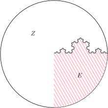
Figure 1. Example 3.6

Given a set $E\subset Z$ with finite $s$-perimeter, we now wish to analyze the codimension $s$ Hausdorff measure of the measure theoretic boundary of $E$. To do so, we will use the hyperbolic filling, where the presence of a $(1,1)$-Poincaré inequality provides us certain potential theoretic tools. In particular, we will use the following lemma, which is a modification of [36, Theorem 5.9]. This can be found for example in [25, Lemma 3.1], where it was proved in greater generality. We include the proof of the particular case pertinent to us for the convenience of the reader.

Lemma 3.7.

Suppose that $(X,d,\mu)$ is a geodesic space, with $\mu$ a doubling measure supporting a $(1,1)$-Poincaré inequality, and let $0<t<1$. Then there exists a constant $C\geq 1$ such that if $r>0$, $E$ and $F$ are subsets of a ball $B(x,r)$, and $\lambda>0$ satisfies

$$\min\{\mathcal{H}^{-t}_{r}(E),\mathcal{H}^{-t}_{r}(F)\}\geq\lambda\frac{\mu(B(x,r))}{r^{t}},$$

then for any function $u\in N^{1,1}(X)$ such that $u=1$ on $E$, $u=0$ on $F$, and each $z\in E\cup F$ such that $z$ is an $L^{1}(\mu)$-Lebesgue point of $u$, we have that

$$\int_{B(x,r)}g_{u}\,d\mu\geq\frac{\lambda}{C}\frac{\mu(B(x,r))}{r},$$

where $g_{u}$ is the minimal $1$-weak upper gradient of $u$.

Proof.

By truncation, we may assume that $0\leq u\leq 1$. If $u_{B(x,r)}\leq 1/2$, then for all $z\in E$, we have that $|u(z)-u_{B(x,r)}|\geq 1/2$. Likewise, if $u_{B(x,r)}>1/2$, then $|u(w)-u_{B(x,r)}|\geq 1/2$ for all $w\in F$. We consider the first case, with the proof of the second case following analogously.

Let $z\in E$, and consider a geodesic $[x,z]$ connecting $x$ to $z$. If $d(x,z)>r/4$, then let $B_{0}:=B(x,r)$, $B_{1}:=B(x,d(x,z)/2)$, and let $B_{2}:=B(x_{2},d(x,z)/2^{2})$, where $x_{2}$ is a point in $[x,z]$ such that $d(x,x_{2})=d(x,z)/2$. Inductively, if $B_{k}:=B(x_{k},d(x,z)/2^{k})$ is such that $x_{k}\in[x,z]$ with $d(x_{k},x_{k-1})=d(x,z)/2^{k-1}$, then we choose a point $x_{k+1}\in[x,z]$ such that $d(x_{k+1},x_{k})=d(x,z)/2^{k}$ and define $B_{k+1}:=B(x_{k+1},d(x,z)/2^{k+1})$. If $d(x,z)\leq r/4$, then set $B_{0}=B(x,r)$, and for each $k\in\mathbb{N}$, let $B_{k}=B(z,2^{-k}r)$. In either case, we obtain a chain of balls $\{B_{k}\}_{k}$ such that for all $k\in\mathbb{N}$, we have that $z\in 3B_{k}$ and $B_{k+1}\subset 2B_{k}\subset B(x,r)$.

Since $z$ is an $L^{1}(\mu)$-Lebesgue point of $u$, we have by the doubling property of $\mu$ and the $(1,1)$-Poincaré inequality, that

$$\frac{1}{2}\leq|u(z)-u_{B(x,r)}|\leq\sum_{k=0}^{\infty}|u_{B_{k+1}}-u_{B_{k}}|\lesssim\sum_{k=0}^{\infty}\fint_{2B_{k}}|u-u_{2B_{k}}|d\mu\lesssim\sum_{k=0}^{\infty}2^{-k}r\fint_{2B_{k}}g_{u}d\mu.$$

Note that the dilation constant in the $(1,1)$-Poincaré inequality is taken to be 1, since $X$ is assumed to be geodesic. Since the series $\sum_{k=0}^{\infty}2^{-k(1-t)}$ converges, there exists $k_{z}\in\mathbb{N}\cup\{0\}$ such that

$$2^{-k_{z}(1-t)}\lesssim 2^{-k_{z}}r\fint_{2B_{k_{z}}}g_{u}d\mu.$$

We then have that

$$\mu(B_{k_{z}})\lesssim 2^{-k_{z}t}r\int_{2B_{k_{z}}}g_{u}d\mu\lesssim r^{1-t}\operatorname{rad}(B_{k_{z}})^{t}\int_{2B_{k_{z}}}g_{u}d\mu.$$

Now, $\{3B_{k_{z}}\}_{z\in E}$ covers $E$, and so by the 5-covering lemma, see [37, Chapter 3], there exists a pairwise disjoint subcollection $\{3B_{i}\}_{i\in I\subset\mathbb{N}}$ such that $\{15B_{i}\}_{i\in I}$ covers $E$. Hence, by the doubling property of $\mu$ and the previous inequality, we have that

$$\mathcal{H}^{-t}_{r}(E)\leq\sum_{i\in I}\frac{\mu(15B_{i})}{(15\operatorname{rad}(B_{i}))^{t}}\lesssim\sum_{i\in I}\frac{\mu(B_{i})}{\operatorname{rad}(B_{i})^{t}}\lesssim\sum_{i\in I}r^{1-t}\int_{2B_{i}}g_{u}d\mu\leq r^{1-t}\int_{B(x,r)}g_{u}d\mu.$$

In the last inequality, we have used the fact that $2B_{i}\subset B(x,r)$ and disjointness of $\{2B_{i}\}_{i\in I}$. By hypothesis, it then follows that

$$\lambda\frac{\mu(B(x,r))}{r}\leq\frac{1}{r^{1-t}}\mathcal{H}^{-t}_{r}(E)\lesssim\int_{B(x,r)}g_{u}d\mu,$$

which completes the proof. ∎

We now prove Theorem 1.2.

Proof of Theorem 1.2.

Fix $0<s<1$ and let $E\subset Z$ be such that $\chi_{E}\in B^{s}_{1,1}(Z,\nu)$. Let $(X,d_{X})$ be the hyperbolic filling of $(Z,d,\nu)$, constructed with parameters $\alpha$, $\tau>1$. Let $\varepsilon=\log\alpha$, and choose $\beta>0$ such that $\beta/\varepsilon=1-s$. Consider the metric $d_{\varepsilon}$ as given by (2.13), and let $\overline{X}_{\varepsilon}$ be the completion with respect to $d_{\varepsilon}$ of the uniformized hyperbolic filling $(X,d_{\varepsilon},\mu_{\beta})$ of $(Z,d,\nu)$, as constructed in Section 2.5. Let $u:=u_{\chi_{E}}\in N^{1,1}(\overline{X}_{\varepsilon},\mu_{\beta})$ be the extension of $\chi_{E}$ given by Theorem 2.15. By Theorem 2.15, we have that $u(z)=\chi_{E}(z)$ for $\nu$-a.e. $z\in Z$, and $\nu$-a.e. $z\in Z$ is an $L^{1}(\mu_{\beta})$-Lebesgue point of $u$. Let $E_{1}:=\{u=1\}\cap Z\setminus N_{u}$ and $E_{0}:=\{u=0\}\cap Z\setminus N_{u}$, where $N_{u}$ is the set of points which are not $L^{1}(\mu_{\beta})$-Lebesgue points of $u$.

Fix $\delta>0$ and $\eta>0$. For each $k\in\mathbb{N}$ let $\partial^{*}_{k}E$ denote the set of points $z\in Z$ such that

$$\limsup_{r\to 0}\frac{\nu(B_{Z}(z,r)\cap E)}{\nu(B_{Z}(z,r))}\geq 2^{-k}\quad\text{ and }\quad\limsup_{r\to 0}\frac{\nu(B_{Z}(z,r)\setminus E)}{\nu(B_{Z}(z,r))}\geq 2^{-k}.$$

Recall that we use the notation $B_{Z}$ to indicate that these are balls with respect to $(Z,d,\nu)$. Letting $N_{\delta}\in\mathbb{N}$ be the smallest positive integer such that $1/N_{\delta}<\delta$. We then have that

(3.8) $$\partial^{*}E=\bigcup_{k=N_{\delta}}^{\infty}\partial^{*}_{k}E,$$

where $\partial^{*}E$ is the measure theoretic boundary of $E$ with respect to $(Z,d,\nu)$.

Fix $k\in\mathbb{N}$ with $k\geq N_{\delta}$. Since $(Z,d,\nu)$ is doubling and $\nu$ satisfies the codimensional relationship (2.14) with respect to $\mu_{\beta}$, it follows that $\mu_{\beta}(Z)=0$. Therefore, since $u\in N^{1,1}(\overline{X}_{\varepsilon},\mu_{\beta})$, there exists $j_{k}\in\mathbb{N}$ such that

(3.9) $$\int_{X_{j_{k}}}g_{u}\,d\mu_{\beta}\leq 2^{-2k}\eta,$$

where $X_{j_{k}}:=\{x\in\overline{X}_{\varepsilon}:\operatorname{dist}(x,\partial X_{\varepsilon})\leq 1/j_{k}\}$ and $g_{u}$ is the minimal $1$-weak upper gradient of $u$ in $\overline{X}_{\varepsilon}$. Recall from Section 2.5 that $(Z,d_{\varepsilon})$ is bi-Lipschitz equivalent to $(Z,d)$. Therefore, there exists a constant $C_{0}\geq 1$ depending only on $\alpha$, $\tau$, and the doubling constant of $\nu$, such that for all $z\in Z$ and $r>0$,

(3.10) $$B_{Z}(z,r)\subset B_{\varepsilon}(z,C_{0}r)\cap Z.$$

Since $u=\chi_{E}$ $\nu$-a.e. in $Z$ and $\nu$-a.e. point in $Z$ is an $L^{1}(\mu_{\beta})$-Lebesgue point of $u$, it follows that for each $\zeta\in\partial^{*}_{k}E$, there exists $0<r_{\zeta,k}<\min\{1/(C_{0}j_{k}),\delta/(5C_{0})\}$ such that

$$\min\{\nu(B_{Z}(\zeta,r_{\zeta,k})\cap E_{1}),\nu(B_{Z}(\zeta,r_{\zeta,k})\cap E_{0})\} =\min\{\nu(B_{Z}(\zeta,r_{\zeta,k})\cap E),\nu(B_{Z}(\zeta,r_{\zeta,k})\setminus E)\}$$

$$\geq\frac{1}{2^{k}}\nu(B_{Z}(\zeta,r_{\zeta,k}))\simeq\frac{1}{2^{k}}\frac{\mu_{\beta}(B_{\varepsilon}(\zeta,r_{\zeta,k}))}{r_{\zeta,k}^{1-s}}.$$

Here we have used (2.14) and the choice $\beta/\varepsilon=1-s$ in the last inequality. By Lemma 2.16, (3.10), and the doubling property of $\mu_{\beta}$, we have that

$$\min \left\{\mathcal{H}^{-(1-s)}_{\mu_{\beta},\,C_{0}r_{\zeta,k}}\left(B_{\varepsilon}(\zeta,C_{0}r_{\zeta,k})\cap E_{1}\right),\mathcal{H}^{-(1-s)}_{\mu_{\beta},\,C_{0}r_{\zeta,k}}(B_{\varepsilon}(\zeta,C_{0}r_{\zeta,k})\cap E_{0})\right\}$$

$$\gtrsim\min\{\nu(B_{\varepsilon}(\zeta,C_{0}r_{\zeta,k})\cap E_{1}),\nu(B_{\varepsilon}(\zeta,C_{0}r_{\zeta,k})\cap E_{0})\}$$

$$\geq\min\{\nu(B_{Z}(\zeta,r_{\zeta,k})\cap E_{1}),\nu(B_{Z}(\zeta,r_{\zeta,k})\cap E_{0})\}\gtrsim\frac{1}{2^{k}}\frac{\mu_{\beta}(B_{\varepsilon}(\zeta,r_{\zeta,k}))}{r_{\zeta,k}^{1-s}}\simeq\frac{1}{2^{k}}\frac{\mu_{\beta}(B_{\varepsilon}(\zeta,C_{0}r_{\zeta,k}))}{(C_{0}r_{\zeta,k})^{1-s}}.$$

Note that $(\overline{X}_{\varepsilon},d_{\varepsilon},\mu_{\beta})$ is geodesic, where $\mu_{\beta}$ is doubling and supports a $(1,1)$-Poincaré inequality, see Section 2.5. Hence, we apply Lemma 3.7 to obtain

$$\int_{B_{\varepsilon}(\zeta,C_{0}r_{\zeta,k})}g_{u}\,d\mu_{\beta}\gtrsim\frac{1}{2^{k}}\frac{\mu_{\beta}(B_{\varepsilon}(\zeta,C_{0}r_{\zeta,k}))}{C_{0}r_{\zeta,k}}.$$

Since $\{B_{\varepsilon}(\zeta,C_{0}r_{\zeta,k})\}_{\zeta\in\partial^{*}_{k}E}$ covers $\partial^{*}_{k}E$, it follows from the 5-covering lemma that there exists a pairwise disjoint subcollection $\{B_{i}\}_{i\in I\subset\mathbb{N}}$ such that $\partial^{*}_{k}E\subset\bigcup_{i\in I}5B_{i}$. Since $r_{\zeta,k}<1/(C_{0}j_{k})$, we have that $B_{i}\subset X_{j_{k}}$ for each $i$. Then, by (3.9), the doubling property of $\mu_{\beta}$, and by $r_{\zeta,k}<\delta/(5C_{0})$, it follows that

$$2^{-2k}\eta>\int_{X_{j_{k}}}g_{u}\,d\mu_{\beta}\geq\sum_{i\in I}\int_{B_{i}}g_{u}\,d\mu_{\beta}\gtrsim\frac{1}{2^{k}}\sum_{i\in I}\frac{\mu_{\beta}(B_{i})}{\operatorname{rad}(B_{i})} \gtrsim\frac{1}{2^{k}}\sum_{i\in I}\frac{\mu_{\beta}(5B_{i})}{\operatorname{rad}(5B_{i})}\geq\frac{1}{2^{k}}\mathcal{H}^{-1}_{\mu_{\beta},\,\delta}(\partial^{*}_{k}E).$$

Hence, from (3.8) we have that

$$\mathcal{H}^{-1}_{\mu_{\beta},\,\delta}(\partial^{*}E)\leq\sum_{k=N_{\delta}}^{\infty}\mathcal{H}^{-1}_{\mu_{\beta},\,\delta}(\partial^{*}_{k}E)\lesssim\eta.$$

As $\delta>0$ and $\eta>0$ are arbitrary, we have from Lemma 2.17 that

$$\mathcal{H}^{-s}_{\nu}(\partial^{*}E)=\mathcal{H}^{-1}_{\mu_{\beta}}(\partial^{*}E)=0.\qed$$

Corollary 1.3 now follows immediately from Theorem 1.1 and Theorem 1.2. As mentioned above, the first inequality in Corollary 1.3 was obtained in the Euclidean setting in [54]. While (1.4) may hold with equality in the above corollary, as is the case with the von Koch snowflake domain, see [48], we provide an example in the next section showing that these inequalities may be strict.

4. Examples

In this section, we demonstrate some sharpness of the above results, and show by example that the converses of Theorem 1.1 and Theorem 1.2 do not hold in general. We do this by constructing a fat Cantor set as follows:

Let $I=[0,1]\subset\mathbb{R}$ be equipped with the Euclidean distance and Lebesgue measure. For a parameter $0<a<1/3$, we remove an open interval $I_{1,1}$ of length $a$ from the center of $I$. Let $C_{1,1}$ and $C_{1,2}$ be the disjoint closed intervals which comprise $I\setminus I_{1,1}$. For the second stage of the construction, we remove an open interval $I_{2,k}$ of length $a^{2}$ from the center of each $C_{1,k}$, $k=1,2$. Let $\{C_{2,k}\}_{k=1}^{4}$ be the remaining closed intervals. Continuing inductively in this manner, for the $j$-th stage of the construction, we remove an open interval $I_{j,k}$ of length $a^{j}$ from the center of each $C_{j-1,k}$, $k=1,\dots,2^{j-1}$, and we let $\{C_{j,k}\}_{k=1}^{2^{j}}$ be the collection of remaining closed intervals. Then for each $1\leq k\leq 2^{j}$, we have that

(4.1) $$\mathcal{H}^{1}(C_{j,k})=\frac{1-3a+a(2a)^{j}}{2^{j}(1-2a)}=:c_{j}.$$

We then define the Cantor set $C_{a}$ by

$$C_{a}:=\bigcap_{j=1}^{\infty}\bigcup_{k=1}^{2^{j}}C_{j,k}=I\setminus\left(\bigcup_{j=1}^{\infty}\bigcup_{k=1}^{2^{j-1}}I_{j,k}\right).$$

Since $0<a<1/3$, we see that

$$\mathcal{H}^{1}(C_{a})=\frac{1-3a}{1-2a}>0.$$

We now relate the Besov energy of the characteristic function of $C_{a}$ to the parameter $a$.

Lemma 4.2.

Let $0<s<1$, $0<a<1/3$, and let $C_{a}$ be constructed as above. Then

$$\|\chi_{C_{a}}\|_{B^{s}_{1,1}(I)}\lesssim\sum_{j=1}^{\infty}(2a^{1-s})^{j}$$

with the comparison constant depending only on $s$.

Proof.

We have that

$$\|\chi_{C_{a}}\|_{B^{s}_{1,1}(I)}=\|\chi_{I\setminus C_{a}}\|_{B^{s}_{1,1}(I)}=\Big{\|}\sum_{j=1}^{\infty}\sum_{k=1}^{2^{j-1}}\chi_{I_{j,k}}\Big{\|}_{B^{s}_{1,1}(I)}\leq\sum_{j=1}^{\infty}\sum_{k=1}^{2^{j-1}}\|\chi_{I_{j,k}}\|_{B^{s}_{1,1}(I)},$$

and for $1\leq j<\infty$ and $1\leq k\leq 2^{j-1}$,

$$\|\chi_{I_{j,k}}\|_{B^{s}_{1,1}(I)}=2\int_{I_{j,k}}\int_{I\setminus I_{j,k}}\frac{1}{|y-x|^{1+s}}dydx.$$

We have that

$$\int_{I_{j,k}}\int_{I\setminus I_{j,k}}\frac{1}{|y-x|^{1+s}}dydx \leq 2\int_{0}^{a^{j}}\int_{a^{j}}^{1}\frac{1}{|y-x|^{1+s}}dydx$$

$$=\frac{2}{s(1-s)}(a^{j(1-s)}+(1-a^{j})^{1-s}-1)\leq\frac{2a^{j(1-s)}}{s(1-s)},$$

and so it follows that

$$\|\chi_{C_{a}}\|_{B^{s}_{1,1}(I)}\leq\frac{2}{s(1-s)}\sum_{j=1}^{\infty}(2a^{1-s})^{j}.\qed$$

Proposition 4.3.

Let $0<s<1$, and let $0<a<1/3$ be such that $a<1/2^{1+s}$. Then

$$\|\chi_{C_{a}}\|_{B^{s}_{1,1}(I)}\simeq\sum_{j=1}^{\infty}(2a^{1-s})^{j},$$

with comparison constant depending only on $s$ and $a$.

Proof.

By Lemma 4.2, we have that

$$\|\chi_{C_{a}}\|_{B^{s}_{1,1}(I)}\lesssim\sum_{j=1}^{\infty}(2a^{1-s})^{j}.$$

To prove the converse inequality, we have that

(4.4) $$\|\chi_{C_{a}}\|_{B^{s}_{1,1}(I)}=2\sum_{j=1}^{\infty}\sum_{k=1}^{2^{j-1}}\int_{I_{j,k}}\int_{C_{a}}\frac{1}{|y-x|^{1+s}}dydx,$$

and for each $1\leq j<\infty$ and $1\leq k\leq 2^{j-1}$,

$$\int_{I_{j,k}}\int_{C_{a}}\frac{1}{|y-x|^{1+s}}dydx=\int_{I_{j,k}}\int_{I\setminus I_{j,k}}\frac{1}{|y-x|^{1+s}}dydx-\sum_{l=1}^{\infty}\sum_{\begin{subarray}{c}m=1,\\ (l,m)\neq(j,k)\end{subarray}}^{2^{l-1}}\int_{I_{j,k}}\int_{I_{l,m}}\frac{1}{|y-x|^{1+s}}dydx.$$

Fix $1\leq j<\infty$ and $1\leq k\leq 2^{j-1}$. Setting $J_{1}:=\int_{I_{j,k}}\int_{I\setminus I_{j,k}}\frac{1}{|y-x|^{1+s}}dydx$, and

$$\sum_{l=1}^{\infty}\sum_{\begin{subarray}{c}m=1,\\ (l,m)\neq(j,k)\end{subarray}}^{2^{l-1}} \int_{I_{j,k}}\int_{I_{l,m}}\frac{1}{|y-x|^{1+s}}dydx$$

$$=\sum_{l=1}^{j}\sum_{\begin{subarray}{c}m=1,\\ (l,m)\neq(j,k)\end{subarray}}^{2^{l-1}}\int_{I_{j,k}}\int_{I_{l,m}}\frac{1}{|y-x|^{1+s}}dydx+\sum_{l=j+1}^{\infty}\sum_{m=1}^{2^{l-1}}\int_{I_{j,k}}\int_{I_{l,m}}\frac{1}{|y-x|^{1+s}}dydx$$

$$=:J_{2}+J_{3},$$

we then have that

(4.5) $$\int_{I_{j,k}}\int_{C_{a}}\frac{1}{|y-x|^{1+s}}dydx=J_{1}-J_{2}-J_{3}.$$

For each $1\leq l\leq j$ and $1\leq m\leq 2^{l-1}$ such that $(l,m)\neq(j,k)$, it follows from the construction that there is at least one closed interval from the collection $\{C_{j,k}\}_{k=1}^{2^{j}}$ separating $I_{j,k}$ and $I_{l,m}$. Hence

$$\operatorname{dist}(I_{j,k},I_{l,m})\geq c_{j}>a^{j},$$

since $0<a<1/3$, where $c_{j}$ is given by (4.1). Letting $I_{j,k}\pm a^{j}$ denote the $a^{j}$-neighborhood of the interval $I_{j,k}$, it then follows that

$$J_{1}-J_{2} =\int_{I_{j,k}}\int_{I\setminus I_{j,k}}\frac{1}{|y-x|^{1+s}}dydx-\sum_{l=1}^{j}\sum_{\begin{subarray}{c}m=1,\\ (l,m)\neq(j,k)\end{subarray}}^{2^{l-1}}\int_{I_{j,k}}\int_{I_{l,m}}\frac{1}{|y-x|^{1+s}}dydx$$

$$\geq\int_{I_{j,k}}\int_{(I_{j,k}\pm a^{j})\setminus I_{j,k}}\frac{1}{|y-x|^{1+s}}dydx$$

(4.6) $$=2\int_{0}^{a^{j}}\int_{a^{j}}^{2a^{j}}\frac{1}{|y-x|^{1+s}}dydx=\frac{4(1-2^{-s})}{s(1-s)}a^{j(1-s)}.$$

To estimate $J_{3}$, fix $l\geq j+1$ and consider the collection of intervals $\{I_{l,m}\}_{m=1}^{2^{l-1}}$. By the construction of $C_{a}$, it follows that for each interval $I_{l,m}$ in this collection, there exist some positive integer $1\leq n_{m}\leq 2^{l}$ such that there are precisely $n_{m}$ closed intervals from the collection $\{C_{l,i}\}_{i=1}^{2^{l}}$ between $I_{j,k}$ and $I_{l,m}$, and so

$$\operatorname{dist}(I_{j,k},I_{l,m})\geq n_{m}c_{l}.$$

From this, we see that

$$\int_{I_{j,k}}\int_{I_{l,m}}\frac{1}{|y-x|^{1+s}}dydx\leq\frac{a^{j}a^{l}}{(n_{m}c_{l})^{1+s}}.$$

Furthermore, for each $1\leq n\leq 2^{l}$, there are at most two intervals from the collection $\{I_{l,m}\}_{m=1}^{2^{l-1}}$ which are separated from $I_{j,k}$ by precisely $n$ closed intervals from $\{C_{l,i}\}_{i=1}^{2^{l}}$. Hence, we overestimate $J_{3}$ as follows:

$$J_{3} =\sum_{l=j+1}^{\infty}\sum_{m=1}^{2^{l-1}}\int_{I_{j,k}}\int_{I_{l,m}}\frac{1}{|y-x|^{1+s}}dydx\leq 2\sum_{l=j+1}^{\infty}\sum_{n=1}^{2^{l}}\frac{a^{j}a^{l}}{(nc_{l})^{1+s}}=2a^{j}\sum_{l=j+1}^{\infty}\frac{a^{l}}{c_{l}^{1+s}}\sum_{n=1}^{2^{l}}\frac{1}{n^{1+s}}$$

We have that

$$\frac{a^{l}}{c_{l}^{1+s}}=a^{l}\left(\frac{2^{l}(1-2a)}{1-3a+a(2a)^{l}}\right)^{1+s}\leq(2^{1+s}a)^{l}\frac{1}{(1-3a)^{1+s}},$$

and so by the assumption that $a<\min\{1/3,1/2^{1+s}\}$, it follows that

$$C_{s,a}:=\sum_{l=1}^{\infty}\frac{a_{l}}{c_{l}^{1+s}}\sum_{n=1}^{\infty}\frac{1}{n^{1+s}}<\infty.$$

Therefore, we have that

(4.7) $$J_{3}\leq 2C_{s,a}a^{j}.$$

Combining (4.5), (4), and (4.7), we have that

$$\int_{I_{j,k}}\int_{C_{a}}\frac{1}{|y-x|^{1+s}}dydx\geq\left(\frac{4(1-2^{-s})}{s(1-s)}-2C_{s,a}a^{js}\right)a^{j(1-s)},$$

and so there exists $N\in\mathbb{N}$, depending on $s$ and $a$ such that

$$\int_{I_{j,k}}\int_{C_{a}}\frac{1}{|y-x|^{1+s}}dydx\geq\frac{2(1-s^{-s})}{s(1-s)}a^{j(1-s)}=:C_{s}a^{j(1-s)}$$

for all $j>N$. By (4.4), we then have that

$$\|\chi_{C_{a}}\|_{B^{s}_{1,1}(I)}\geq 2\sum_{j=1}^{N}\sum_{k=1}^{2^{j-1}}\int_{I_{j,k}}\int_{C_{a}}\frac{1}{|y-x|^{1+s}}dydx+C_{s}\sum_{j=N+1}^{\infty}(2a^{1-s})^{j}.$$

For each $1\leq j\leq N$ and $1\leq k\leq 2^{j-1}$, there exists $C_{j,k}>0$ such that

$$2\int_{I_{j,k}}\int_{C_{a}}\frac{1}{|y-x|^{1+s}}dydx\geq C_{j,k}a^{j(1-s)}.$$

Such a $C_{j,k}$ exists since $\mathcal{H}^{1}(C_{a})>0$. Therefore, letting

$$C:=\min\{C_{s},C_{j,k}:1\leq j\leq N,\,1\leq k\leq 2^{j-1}\},$$

which depends only on $s$ and $a$, we have that

$$\|\chi_{C_{a}}\|_{B^{s}_{1,1}(I)}\geq C\sum_{j=1}^{\infty}(2a^{1-s})^{j}.\qed$$

By using Proposition 4.3, we can now provide examples illustrating the sharpness of Theorem 1.2, and that the converses of Theorem 1.2 and Theorem 1.1 do not hold in general.

Example 4.8.

For each $0<a<1/3$, consider the Cantor set $C_{a}$ constructed above. The regularized boundary of $C_{a}$ is given by

$$\partial^{+}C_{a}=C_{a}.$$

Then,

$$\mathcal{H}^{1}(\partial^{+}C_{a})=\mathcal{H}^{1}(C_{a})=\frac{1-3a}{1-2a}>0,$$

and so $\mathcal{H}^{-s}(\partial^{+}C_{a})=\infty$ for all $0<s<1$. However, by Proposition 4.3, we can choose $0<a<1/3$ and $0<s<1$ such that $\chi_{C_{a}}\in B^{s}_{1,1}(I)$. This shows that Theorem 1.2 is sharp in the sense that we cannot strengthen the conclusion by replacing $\partial^{*}E$ with $\partial^{+}E$, or even replacing $\mathcal{H}^{-s}(\partial^{*}E)=0$ with $\mathcal{H}^{-s}(\partial^{+}E)<\infty$.

Example 4.9.

For each $0<a<1/3$, consider the Cantor set $C_{a}$, and let $\{x_{i}\}_{i\in\mathbb{N}}$ be the endpoints of the open intervals $I_{j,k}$ considered above. Since $\mathcal{H}^{1}(C_{a})>0$, we see from the construction that

$$\limsup_{r\to 0^{+}}\frac{\mathcal{H}^{1}(B(x,r)\setminus C_{a})}{\mathcal{H}^{1}(B(x,r))}=0$$

for all $x\in C_{a}\setminus\{x_{i}\}_{i\in\mathbb{N}}.$ Therefore, $\partial^{*}C_{a}=\{x_{i}\}_{i\in\mathbb{N}}$, and as a countable set, it follows that

$$\mathcal{H}^{-s}(\partial^{*}C_{a})=0$$

for all $0<s<1$.

Now, fix $0<a_{0}<1/4$. We can then choose $0<s_{0}<1$ sufficiently close to $1$ so that $2a_{0}^{1-s_{0}}>1$. Since $a_{0}^{1/(1+s_{0})}<a_{0}^{1/2}<1/2$, the hypotheses of Proposition 4.3 are satisfied, and so $\chi_{C_{a_{0}}}\not\in B^{s_{0}}_{1,1}(I)$. However, by the above discussion, we have that $\mathcal{H}^{-s_{0}}(\partial^{*}C_{a_{0}})=0$. Thus the converse of Theorem 1.2 does not hold in general.

Example 4.10.

Let $0<a<1/3$ and $0<t<1$. For $r>0$, consider a countable cover $\{B(y_{j},r)\}_{j\in\mathbb{N}}$ of $\partial^{*}C_{a}=\{x_{i}\}_{i\in\mathbb{N}}$, such that $y_{j}\in\partial^{*}C_{a}$ for each $j\in\mathbb{N}$. If $z_{1}\in C_{a}\setminus\bigcup_{j}B(y_{j},r)$, then by the density of $\partial^{*}C_{a}$ in $C_{a}$, we have that $\operatorname{dist}(z_{1},\bigcup_{j}B(y_{j},r))=0$. Hence if $z_{2}\in C_{a}\setminus\bigcup_{j}B(y_{j},r)$ such that $z_{1}\neq z_{2}$, then $d(z_{1},z_{2})\geq 2r$. Therefore $C_{a}\setminus\bigcup_{j}B(y_{j},r)$ is a finite set. Thus, we have that

$$\sum_{j}r^{-t}\mathcal{H}^{1}(B(y_{j},r))\geq r^{-t}\mathcal{H}^{1}(C_{a}),$$

and so since $\{B(y_{j},r)\}_{j\in\mathbb{N}}$ is arbitrary, we have that $\mathcal{M}^{-t}_{r}(\partial^{*}C_{a})\geq r^{-t}\mathcal{H}^{1}(C_{a})$. Since $\mathcal{H}^{1}(C_{a})>0$, it follows that $\underline{\mathcal{M}}^{-t}(\partial^{*}C_{a})=\infty$. However by Proposition 4.3, we can choose $0<a<1/3$ and $0<s<1/2$ so that $\chi_{C_{a}}\in B^{s}_{1,1}(I)$. Therefore, the converse to Theorem 1.1 does not hold in general for any $0<t<1$, nor even with the weaker conclusion that $\underline{\mathcal{M}}^{-t}(\partial^{*}E)<\infty$.

Example 4.11.

It was shown in [48] that the von Koch snowflake domain $K\subset\mathbb{R}^{2}$ is such that

$$\overline{\operatorname{codim}}_{\mathcal{M}}(\partial^{+}K)=\operatorname{codim}_{F}(K)=\operatorname{codim}_{\mathcal{H}}(\partial^{*}K)=2-\log 4/\log 3.$$

That is, (1.4) holds with equality in some cases. However, the fat Cantor sets constructed above show that these inequalities may be strict. For example, let $a=1/4$ and consider $C_{a}$. By Proposition 4.3, we see that $\chi_{C_{a}}\in B^{s}_{1,1}(I)$ if and only if $0<s<1/2$, and so $\operatorname{codim}_{F}(C_{a})=1/2$. However, $\mathcal{H}^{-s}(\partial^{*}C_{a})=0$ and $\overline{\mathcal{M}}^{-s}(\partial^{+}C_{a})=\infty$ for all $0<s<1$. Hence, we have that

$$0=\overline{\operatorname{codim}}_{\mathcal{M}}(\partial^{+}C_{a})<\operatorname{codim}_{F}(C_{a})<\operatorname{codim}_{\mathcal{H}}(\partial^{*}C_{a})=1.$$

5. Existence of minimizers of $\mathcal{J}_{\Omega}^{s}$

Throughout this section, we assume that $(X,d,\mu)$ is a metric measure space, with $\mu$ a doubling Borel regular measure. Let $\Omega\subset X$ be a bounded domain, that is, a bounded connected open set. Without loss of generality, we may assume that $X\setminus\Omega\neq\varnothing$. Otherwise, the existence results of this section hold trivially. Let $F\subset X$, and let $0<s<1$. We consider the functional

$$\mathcal{J}_{\Omega}^{s}(E):=L_{s}(E\cap\Omega,X\setminus E)+L_{s}(E\setminus\Omega,\Omega\setminus E)$$

and the associated minimization problem defined in Section 2.6 and Definition 2.22, and prove existence of minimizers of $\mathcal{J}_{\Omega}^{s}$ by the direct method of calculus of variations. We first note that $\mathcal{J}_{\Omega}^{s}$ is lower semicontinuous with respect to $L^{1}$-convergence by Fatou’s lemma, see [15, Proposition 3.1].

Proposition 5.1.

If $E_{k}$ and $E$ are subsets of $X$ such that $\chi_{E_{k}}\to\chi_{E}$ in $L^{1}_{\text{loc}}(X)$ as $k\to\infty$, then

$$\mathcal{J}_{\Omega}^{s}(E)\leq\liminf_{k\to\infty}\mathcal{J}_{\Omega}^{s}(E_{k}).$$

The following compactness theorem is an adaption of [18, Theorem 7.1], proved there in $\mathbb{R}^{n}$. To prove the result in the doubling metric measure space setting, we will use the discrete convolution technique, obtained from the Lipschitz partition of unity given by Lemmas 2.3 and 2.4.

Theorem 5.2.

Let $\Omega\subset X$ be an open set. Let $\mathcal{F}$ be a family of functions on $\Omega$ such that for all compact sets $K\subset\Omega$,

(5.3) $$\sup_{f\in\mathcal{F}}\|f\|_{L^{1}(K)}<\infty,$$

and also that

(5.4) $$\sup_{f\in\mathcal{F}}\|f\|_{B^{s}_{1,1}(K)}<\infty.$$

Then, for any sequence $\{f_{k}\}_{k}\subset\mathcal{F}$, there exists $f\in L^{1}_{\text{loc}}(\Omega)$ and a subsequence, not relabeled, so that $f_{k}\to f$ in $L^{1}_{\text{loc}}(\Omega)$ and pointwise $\mu$-a.e. in $\Omega$.

Proof.

Let $\widetilde{\Omega}\Subset\Omega$, and let $K\subset\Omega$ be compact such that $\widetilde{\Omega}\subset K$. For each $0<\varepsilon<\operatorname{dist}(K,X\setminus\Omega)/4$, there exists by Lemma 2.3, a countable cover $\{B_{i}^{\varepsilon}\}_{i\in I\subset\mathbb{N}}$ of $X$ by balls of radius $\varepsilon$ with bounded overlap, such that collection $\{\frac{1}{5}B_{i}^{\varepsilon}\}_{i\in I}$ is pairwise disjoint. Let $\{\varphi_{i}^{\varepsilon}\}_{i\in I}$ be a Lipschitz partition of unity subordinate to this cover, given by Lemma 2.4.

Let $J:=\{i\in I:B_{i}^{\varepsilon}\cap K\neq\varnothing\}$. Since $K$ is bounded and since $\{\frac{1}{5}B_{i}^{\varepsilon}\}_{i\in J}$ is pairwise disjoint, the doubling property of $\mu$ ensures that $J$ is a finite set. Thus, there exists $N_{\varepsilon}\in\mathbb{N}$ so that, relabeling if necessary, we can denumerate this collection as follows:

$$\{B_{i}^{\varepsilon}\}_{i\in J}=\{B_{i}^{\varepsilon}\}_{i=1}^{N_{\varepsilon}}.$$

By Lemma 2.4, it follows that for each $x\in K$,

(5.5) $$\sum_{i=1}^{N_{\varepsilon}}\varphi_{i}^{\varepsilon}(x)=\sum_{i\in I}\varphi_{i}^{\varepsilon}(x)=1.$$

By the above upper bound on $\varepsilon$, we can choose a compact set $\widetilde{K}\Subset\Omega$, independent of $\varepsilon$, such that $\bigcup_{i=1}^{N_{\varepsilon}}2B_{i}^{\varepsilon}\subset\widetilde{K}$. For each $f\in\mathcal{F}$, we define the discrete convolution $f_{\varepsilon}$ of $f$ by

$$f_{\varepsilon}=\sum_{i=1}^{N_{\varepsilon}}f_{B_{i}^{\varepsilon}}\varphi_{i}^{\varepsilon}.$$

We also define the vector

$$R(f)=\left(\int_{B_{1}^{\varepsilon}}f\,d\mu,\dots,\int_{B_{N^{\varepsilon}}^{\varepsilon}}f\,d\mu\right)\in\mathbb{R}^{N_{\varepsilon}}.$$

By the bounded overlap of the cover $\{B_{i}^{\varepsilon}\}_{i=1}^{N_{\varepsilon}}$ and (5.3), we have that

$$\|R(f)\|_{\ell^{1}}\leq\sum_{i=1}^{N_{\varepsilon}}\int_{B_{i}^{\varepsilon}}|f|d\mu\lesssim\int_{\bigcup_{i=1}^{N_{\varepsilon}}B^{\varepsilon}_{i}}|f|d\mu\leq\int_{\widetilde{K}}|f|d\mu\leq\sup_{f\in\mathcal{F}}\|f\|_{L^{1}(\widetilde{K})}<\infty.$$

Therefore, we have that $R(\mathcal{F})$ is a totally bounded set in $(\mathbb{R}^{N_{\varepsilon}},\|\cdot\|_{\ell^{1}})$, and so for every $\eta>0$, there exists $M_{\eta}\in\mathbb{N}$ and $b_{1},\dots,b_{M_{\eta}}\in\mathbb{R}^{N_{\varepsilon}}$ such that for every $f\in\mathcal{F}$, there exists $j\in\{1,\dots,M_{\eta}\}$ such that

(5.6) $$\|R(f)-b_{j}\|_{1}<\eta.$$

Let $\eta:=\varepsilon/(N_{\varepsilon}+1)$. For each $j\in\{1,\dots,M_{\eta}\}$, let $b_{j}=(b_{1,j},\dots,b_{N_{\varepsilon},j})$, and define $\beta_{j}:\Omega\to\mathbb{R}$ by

$$\beta_{j}=\sum_{i=1}^{N_{\varepsilon}}\frac{b_{i,j}}{\mu(B_{i}^{\varepsilon})}\varphi_{i}^{\varepsilon}.$$

For $f\in\mathcal{F}$, let $j\in\{1,\dots,M_{\eta}\}$ be such that (5.6) holds. We then have that

(5.7) $$\|f-\beta_{j}\|_{L^{1}(K)}\leq\|f-f_{\varepsilon}\|_{L^{1}(K)}+\|f_{\varepsilon}-\beta_{j}\|_{L^{1}(K)}.$$

By (5.5), we have that

$$\|f-f_{\varepsilon}\|_{L^{1}(K)}\leq\sum_{k=1}^{N_{\varepsilon}}\int_{B_{k}^{\varepsilon}\cap K}|f-f_{\varepsilon}|d\mu\leq\sum_{k=1}^{N_{\varepsilon}}\sum_{i=1}^{N_{\varepsilon}}\int_{B_{k}^{\varepsilon}\cap K}|f(x)-f_{B_{i}^{\varepsilon}}|\varphi_{i}^{\varepsilon}(x)d\mu(x).$$

Letting $I_{k}:=\{i\in\{1,\dots,N_{\varepsilon}\}:2B_{i}^{\varepsilon}\cap B_{k}^{\varepsilon}\neq\varnothing\}$, we have that

$$\|f-f_{\varepsilon}\|_{L^{1}(K)}\leq\sum_{k=1}^{N_{\varepsilon}}\sum_{i\in I_{k}}\int_{B_{k}^{\varepsilon}\cap K}|f-f_{B_{i}^{\varepsilon}}|d\mu\leq\sum_{k=1}^{N_{\varepsilon}}\sum_{i\in I_{k}}\int_{B_{k}^{\varepsilon}}\fint_{B_{i}^{\varepsilon}}|f(x)-f(y)|d\mu(y)d\mu(x).$$

For $x\in B_{k}^{\varepsilon}$ and $i\in I_{k}$, we then have by the doubling property of $\mu$ that

$$\fint_{B_{i}^{\varepsilon}}|f(x)-f(y)|d\mu(y) \lesssim\varepsilon^{s}\frac{\mu(B(x,5\varepsilon))}{\mu(B_{i}^{\varepsilon})}\int_{B_{i}^{\varepsilon}}\frac{|f(y)-f(x)|}{d(x,y)^{s}\mu(B(x,d(x,y)))}d\mu(y)$$

$$\lesssim\varepsilon^{s}\int_{B_{i}^{\varepsilon}}\frac{|f(y)-f(x)|}{d(x,y)^{s}\mu(B(x,d(x,y)))}d\mu(y).$$

Substituting this into the previous expression, we have by bounded overlap of $\{B_{i}^{\varepsilon}\}_{i=1}^{N_{\varepsilon}}$,

$$\|f-f_{\varepsilon}\|_{L^{1}(K)} \lesssim\varepsilon^{s}\sum_{k=1}^{N_{\varepsilon}}\sum_{i\in I_{k}}\int_{B_{k}^{\varepsilon}}\int_{B_{i}^{\varepsilon}}\frac{|f(y)-f(x)|}{d(x,y)^{s}\mu(B(x,d(x,y)))}d\mu(y)d\mu(x)$$

$$\lesssim\varepsilon^{s}\int_{\widetilde{K}}\int_{\widetilde{K}}\frac{|f(y)-f(x)|}{d(x,y)^{s}\mu(B(x,d(x,y)))}d\mu(y)d\mu(x)$$

(5.8) $$\leq\varepsilon^{s}\sup_{f\in\mathcal{F}}\|f\|_{B^{s}_{1,1}(\widetilde{K})}.$$

Since we have chosen $j\in\{1,\dots,M_{\eta}\}$ so that (5.6) holds, we have from the doubling property of $\mu$ and choice of $\eta$ that

$$\|f_{\varepsilon}-\beta_{j}\|_{L^{1}(K)}\leq\sum_{k=1}^{N_{\varepsilon}}\int_{B_{k}^{\varepsilon}}|f_{\varepsilon}-\beta_{j}|d\mu \leq\sum_{k=1}^{N_{\varepsilon}}\int_{B_{k}^{\varepsilon}}\sum_{i=1}^{N_{\varepsilon}}|f_{B_{i}^{\varepsilon}}-b_{i,j}/\mu(B_{i}^{\varepsilon})|\varphi_{i}^{\varepsilon}(x)d\mu(x)$$

$$\leq\sum_{k=1}^{N_{\varepsilon}}\int_{B_{k}^{\varepsilon}}\sum_{i\in I_{k}}\frac{1}{\mu(B_{i}^{\varepsilon})}\left|\int_{B_{i}^{\varepsilon}}f\,d\mu-b_{i,j}\right|d\mu(x)$$

$$\lesssim\sum_{k=1}^{N_{\varepsilon}}\fint_{B_{k}^{\varepsilon}}\sum_{i=1}^{N_{\varepsilon}}\left|\int_{B_{i}^{\varepsilon}}f\,d\mu-b_{i,j}\right|d\mu(x)$$

$$=\sum_{k=1}^{N_{\varepsilon}}\fint_{B_{k}^{\varepsilon}}\|R(f)-b_{j}\|_{\ell^{1}}\,d\mu<N_{\varepsilon}\eta<\varepsilon.$$

Combining this estimate with (5) and (5.7), we have that

$$\|f-\beta_{j}\|_{L^{1}(\widetilde{\Omega})}\leq\|f-\beta_{j}\|_{L^{1}(K)}\lesssim\varepsilon^{s}\sup_{f\in\mathcal{F}}\|f\|_{B^{s}_{1,1}(\widetilde{K})}+\varepsilon.$$

Recall that the compact set $\widetilde{K}$ is chosen independently of $\varepsilon>0$, and

$$C:=\sup_{f\in\mathcal{F}}\|f\|_{B^{s}_{1,1}(\widetilde{K})}<\infty$$

by (5.4). Therefore, we have shown that for all $\varepsilon>0$, there exists $M_{\varepsilon}\in\mathbb{N}$ and $\beta_{1},\dots,\beta_{M_{\varepsilon}}\in L^{1}(\widetilde{\Omega})$ such that for all $f\in\mathcal{F}$, there exists $j\in\{1,\dots,M_{\varepsilon}\}$ such that

$$\|f-\beta_{j}\|_{L^{1}(\widetilde{\Omega})}\lesssim C\varepsilon^{s}+\varepsilon,$$

with comparison constant depending only on $s$ and the doubling constant of $\mu$. That is, $\mathcal{F}$ is totally bounded, and hence precompact, in $L^{1}(\widetilde{\Omega})$, by completeness of $L^{1}(\widetilde{\Omega})$.

Let $\{f_{k}\}_{k}\subset\mathcal{F}$. Let $\Omega=\bigcup_{i=1}^{\infty}\Omega_{i}$ be an exhaustion of $\Omega$ by an increasing sequence of open sets $\Omega_{i}\Subset\Omega$. Since $\mathcal{F}$ is precompact in $L^{1}(\Omega_{1})$, there exists a subsequence $\{f_{1,k}\}_{k}\subset\{f_{k}\}_{k}$ and $g_{1}$ such that $f_{1,k}\to g_{1}$ in $L^{1}(\Omega_{1})$ as $k\to\infty$. We choose $k_{1}\in\mathbb{N}$ such that

$$\|f_{1,k_{1}}-g_{1}\|_{L^{1}(\Omega_{1})}<2^{-1}.$$

Inductively, for $i\geq 2$, there exists by precompactness of $\mathcal{F}$ on $\Omega_{i}$, a subsequence $\{f_{i,k}\}_{k}\subset\{f_{i-1,k}\}_{k=k_{i-1}}^{\infty}$ and a function $g_{i}$ such that $f_{i,k}\to g_{i}$ in $L^{1}(\Omega_{i})$ as $k\to\infty$. Furthermore, there exists $k_{i}\in\mathbb{N}$ such that

$$\|f_{i,k_{i}}-g_{i}\|_{L^{1}(\Omega_{i})}<2^{-i}.$$

Since the subsequences are nested in this manner, we have that $g_{i}=g_{i-1}$ $\mu$-a.e. on $\Omega_{i-1}$. We then define $f\in L^{1}_{\text{loc}}(\Omega)$ by $f(x)=g_{i}(x)$ if $x\in\Omega_{i}$. We claim that $f_{i,k_{i}}\to f$ in $L^{1}_{\text{loc}}(\Omega)$ and pointwise $\mu$-a.e. in $\Omega$. Indeed, for $i_{0}\in\mathbb{N}$, $\{f_{i,k_{i}}\}_{i=i_{0}}^{\infty}$ is a subsequence of $\{f_{i_{0},k}\}_{k}$, and $f_{i_{0},k}\to f$ in $L^{1}(\Omega_{i_{0}})$ as $k\to\infty$. Moreover, by the monotone convergence theorem and our choice of $k_{i}$, we have that

$$\int_{\Omega_{i_{0}}}\sum_{i=i_{0}}^{\infty}|f_{i,k_{i}}-f|d\mu=\sum_{i=i_{0}}^{\infty}\int_{\Omega_{i_{0}}}|f_{i,k_{i}}-f|d\mu<\sum_{i=i_{0}}^{\infty}2^{-i}<\infty.$$

Hence, $\sum_{i=i_{0}}^{\infty}|f_{i,k_{i}}-f|<\infty$ $\mu$-a.e. in $\Omega_{i_{0}}$, and so $f_{i,k_{i}}\to f$ pointwise $\mu$-a.e. in $\Omega_{i_{0}}$ as $i\to\infty$. Since $i_{0}$ is arbitrary, and $\Omega=\bigcup_{i=1}^{\infty}\Omega_{i}$ with $\Omega_{i}\Subset\Omega$, this concludes the proof. ∎

We define the following collection of measurable sets:

$$\mathcal{A}(F):=\{E\subset X:E\setminus\Omega=F\setminus\Omega,\,\mathcal{J}_{\Omega}^{s}(E)<\infty\}.$$

Theorem 5.9.

If $\mathcal{A}(F)\neq\varnothing$, then there exists a minimizer of $\mathcal{J}_{\Omega}^{s}$.

Proof.

Since $\mathcal{A}(F)\neq\varnothing$, we have that $\beta:=\inf\{\mathcal{J}_{\Omega}^{s}(E):E\in\mathcal{A}(F)\}<\infty$. Let $\{E_{k}\}_{k\in\mathbb{N}}$ be a sequence in $\mathcal{A}(F)$ such that $\mathcal{J}_{\Omega}^{s}(E_{k})\to\beta$ as $k\to\infty$. Hence we have that

$$\sup_{k}\left(\|\chi_{E_{k}}\|_{L^{1}(\Omega)}+\|\chi_{E_{k}}\|_{B^{s}_{1,1}(\Omega)}\right)<\infty$$

as $\Omega$ is bounded, and so by Theorem 5.2, there exists $f\in L^{1}_{\text{loc}}(\Omega)$ and a subsequence $\{E_{k}\}_{k}$, not relabeled, such that $\chi_{E_{k}}\to f$ in $L^{1}_{\text{loc}}(\Omega)$ and pointwise $\mu$-a.e. in $\Omega$ as $k\to\infty$. Thus, we can take $f=\chi_{\widetilde{E}}$ for some set $\widetilde{E}\subset\Omega$.

Let $\Omega=\bigcup_{i=1}^{\infty}\Omega_{i}$ be an exhaustion of $\Omega$ by an increasing sequence of open sets $\Omega_{i}\Subset\Omega$, and let $\varepsilon>0$. Since $\Omega$ is bounded, there exists $i\in\mathbb{N}$ such that $\mu(\Omega\setminus\Omega_{i})<\varepsilon$. We then have that

$$\int_{\Omega}|\chi_{E_{k}}-\chi_{\widetilde{E}}|d\mu=\int_{\Omega_{i}}|\chi_{E_{k}}-f|d\mu+\int_{\Omega\setminus\Omega_{i}}|\chi_{E_{k}}-\chi_{\widetilde{E}}|d\mu<\int_{\Omega_{i}}|\chi_{E_{k}}-f|d\mu+\varepsilon.$$

Since $\chi_{E_{k}}\to f$ in $L^{1}_{\text{loc}}(\Omega)$, we have that $\chi_{E_{k}}\to\chi_{\widetilde{E}}$ in $L^{1}(\Omega)$. Letting $E=\widetilde{E}\cup(F\setminus\Omega)$, we then have that $\chi_{E_{k}}\to\chi_{E}$ in $L^{1}_{\text{loc}}(X)$, as $\chi_{E}=\chi_{E_{k}}=\chi_{F}$ in $X\setminus\Omega$ for all $k$. By Proposition 5.1, it follows that

$$\mathcal{J}_{\Omega}^{s}(E)\leq\liminf_{k\to\infty}\mathcal{J}_{\Omega}^{s}(E_{k})=\beta<\infty.$$

As $E\in\mathcal{A}(F)$, it follows that $E$ is a minimizer of $\mathcal{J}_{\Omega}^{s}$. ∎

Remark 5.10.

We note that Theorem 1.1 gives us a sufficient condition on $\Omega$ for existence of solutions. Namely, if $(X,d,\mu)$ is a doubling metric measure space satisfying the LLC-1 condition, and if $\Omega\subset X$ is bounded and there exists $t>s$ such that $\overline{\mathcal{M}}^{-t}(\partial^{+}\Omega)<\infty$, then $\mathcal{A}(F)\neq\emptyset$. Indeed, by Theorem 1.1,

$$\mathcal{J}_{\Omega}^{s}(F\setminus\Omega)=L_{s}(F\setminus\Omega,\Omega)\leq L_{s}(X\setminus\Omega,\Omega)\simeq\|\chi_{\Omega}\|_{B^{s}_{1,1}(X)}<\infty,$$

and so $F\setminus\Omega\in\mathcal{A}(F)$. We compare this to the existence result from [15] in $\mathbb{R}^{n}$, where the assumption that $\Omega\subset\mathbb{R}^{n}$ is a bounded Lipschitz domain ensures that $\|\chi_{\Omega}\|_{B^{s}_{1,1}(\mathbb{R}^{n})}<\infty$.

6. Regularity of minimizers of $\mathcal{J}_{\Omega}^{s}$

Throughout this section, we assume that $(X,d,\mu)$ is a connected metric measure space, with $\mu$ a doubling Borel regular measure. We let $0<s<1$ and assume that $\Omega\subset X$ is a bounded domain. As before, we may assume, without loss of generality, that $X\setminus\Omega\neq\varnothing$. Otherwise, constant functions are the only minimizers of $\mathcal{J}_{\Omega}^{s}$, and the results in this section hold trivially. We prove uniform density estimates and porosity of minimizers of $\mathcal{J}_{\Omega}^{s}$, analogous to the results obtained in the Euclidean setting in [15, Theorem 4.1,Corollary 4.3]. In the metric setting, similar regularity results were obtained in [42, Theorems 4.2,5.2] for minimizers of the (local) perimeter functional when the space is doubling and supports a $(1,1)$-Poincaré inequality. We emphasize here that the energy functional $\mathcal{J}_{\Omega}^{s}$ is nonlocal, unlike in [42].

6.1. Uniform density estimates

In [42], the authors obtained uniform density estimates for the (local) perimeter minimizers by means of the $(1,1)$-Poincaré inequality and the De Giorgi method. Since we are concerned with the nonlocal case, we do not need to assume that $(X,d,\mu)$ supports a $(1,1)$-Poincaré inequality. Instead, we will make use of the fractional Poincaré inequality given by Theorem 2.10, which does not impose the geometric restrictions that the $(1,1)$-Poincaré inequality imposes on the metric measure space. In the statement of Theorem 2.10, it is assumed that $(X,d,\mu)$ is reverse doubling; since we assume that $X$ is connected and $\mu$ is doubling, this condition is satisfied [7, Corollary 3.8].

Proof of Theorem 1.5.

Let $E\subset X$ be a minimizer of $\mathcal{J}_{\Omega}^{s}$. Modifying $E$ by a set of measure zero if necessary, we may assume by Lemma 2.7 that $\mu(B(x,r)\cap E)>0$ and $\mu(B(x,r)\setminus E)>0$ for each $x\in\partial E$ and $r>0$. Note that such a modification on a set of measure zero does not affect the property of being a minimizer. Let $x_{0}\in\partial E\cap\Omega$ and $R_{0}>0$ be such that $B(x_{0},2R_{0})\subset\Omega$. We prove the first inequality of (1.6), as the second inequality follows from the first and the fact that the complement of a minimizer of $\mathcal{J}_{\Omega}^{s}$ is also a minimizer.

Let $z\in\Omega$ and $R>0$ be such that $B(z,4R)\subset\Omega.$ For each $0<r<R$, let

$$u=\chi_{B(z,r)\cap E}.$$

Since $X$ is connected and $X\setminus\Omega\neq\varnothing$, there exists $y\in\partial B(z,3r/2)$, and so $B(y,r/2)\subset B(z,2r)$ and $B(y,r/2)\cap B(z,r)=\varnothing$. Since $\mu$ is doubling, it then follows that

(6.1) $$\frac{\mu(B(z,2r)\cap\{|u|>0\})}{\mu(B(z,2r))}\leq\frac{\mu(B(z,r))}{\mu(B(z,2r))}\leq\frac{\mu(B(z,r))}{\mu(B(z,r))+\mu(B(y,r/2))}\leq 1/(1+C_{\mu}^{-3})<1.$$

By the doubling property of $\mu$ and by applying Lemma 2.11, we obtain

$$\left(\frac{\mu(B(z,r)\cap E)}{\mu(B(z,r))}\right)^{(Q-s)/Q} \lesssim\left(\fint_{B(z,2r)}|u|^{Q/(Q-s)}d\mu\right)^{(Q-s)/Q}$$

$$\lesssim\frac{r^{s}}{\mu(B(z,r))}\int_{B(z,4r)}\int_{B(z,4r)}\frac{|u(x)-u(y)|}{d(x,y)^{s}\mu(B(x,d(x,y))}d\mu(y)d\mu(x)$$

$$\lesssim\frac{r^{s}}{\mu(B(z,r))}\int_{B(z,r)\cap E}\int_{X\setminus(B(z,r)\cap E)}\frac{d\mu(y)\,d\mu(x)}{d(x,y)^{s}\mu(B(x,d(x,y))}$$

$$=\frac{r^{s}}{\mu(B(z,r))}L_{s}(B(z,r)\cap E,X\setminus(B(z,r)\cap E)).$$

Setting $A=B(z,r)\cap E$, we have by Lemma 2.23 and (2.19) that

$$L_{s}(A,X\setminus A)=L_{s}(A,X\setminus E)+L_{s}(A,E\setminus A)\lesssim L_{s}(A,E\setminus A)\leq L_{s}(A,X\setminus B(z,r)).$$

Substituting this into the above inequality then yields

$$\left(\frac{\mu(B(z,r)\cap E)}{\mu(B(z,r))}\right)^{(Q-s)/Q}\lesssim\frac{r^{s}}{\mu(B(z,r))}\int_{B(z,r)\cap E}\int_{X\setminus B(z,r)}\frac{d\mu(y)\,d\mu(x)}{d(x,y)^{s}\mu(B(x,d(x,y))}.$$

Setting $r_{x}:=r-d(z,x)$ for each $x\in E\cap B(z,r)$, we have by the doubling property of $\mu$ that

$$\int_{X\setminus B(z,r)}\frac{d\mu(y)}{d(x,y)^{s}\mu(B(x,d(x,y))} \leq\int_{X\setminus B(x,r_{x})}\frac{d\mu(y)}{d(x,y)^{s}\mu(B(x,d(x,y))}$$

$$=\sum_{m=0}^{\infty}\int_{B(x,2^{m+1}r_{x})\setminus B(x,2^{m}r_{x})}\frac{d\mu(y)}{d(x,y)^{s}\mu(B(x,d(x,y))}$$

$$\lesssim\frac{1}{(r-d(z,x))^{s}}.$$

Substituting this into the previous expression, we obtain

$$\frac{\mu(B(z,r))}{r^{s}}\left(\frac{\mu(B(z,r)\cap E)}{\mu(B(z,r))}\right)^{(Q-s)/Q} \lesssim\int_{B(z,r)\cap E}\frac{1}{(r-d(z,x))^{s}}d\mu(x).$$

Integrating both sides of the above expression with respect to $r$, and using Tonelli’s theorem gives

$$\int_{R/2}^{R}\frac{\mu(B(z,r))}{r^{s}}\left(\frac{\mu(B(z,r)\cap E)}{\mu(B(z,r))}\right)^{(Q-s)/Q}dr \lesssim\int_{0}^{R}\int_{B(z,r)\cap E}\frac{1}{(r-d(z,x))^{s}}d\mu(x)dr$$

$$=\int_{0}^{R}\int_{B(z,R)}\frac{\chi_{E}(x)\chi_{B(z,r)}(x)}{(r-d(z,x))^{s}}d\mu(x)dr$$

$$=\int_{B(z,R)}\chi_{E}(x)\int_{0}^{R}\frac{\chi_{B(z,r)}(x)}{(r-d(z,x))^{s}}drd\mu(x)$$

$$=\int_{B(z,R)}\chi_{E}(x)\int_{d(z,x)}^{R}\frac{1}{(r-d(z,x))^{s}}drd\mu(x)$$

$$\lesssim R^{1-s}\mu(B(z,R)\cap E).$$

By the doubling property of $\mu$, we estimate the left-hand side of the above expression from below by

$$\int_{R/2}^{R}\frac{\mu(B(z,r))}{r^{s}}\left(\frac{\mu(B(z,r)\cap E)}{\mu(B(z,r))}\right)^{(Q-s)/Q}dr \gtrsim R^{1-s}\mu(B(z,R))\left(\frac{\mu(B(z,R/2)\cap E)}{\mu(B(z,R/2))}\right)^{(Q-s)/Q}.$$

Combining this with the previous expression, we obtain

(6.2) $$\left(\frac{\mu(B(z,R/2)\cap E)}{\mu(B(z,R/2))}\right)^{(Q-s)/Q} \leq C_{0}\frac{\mu(B(z,R)\cap E)}{\mu(B(z,R))}$$

for all $z\in\Omega$ and $R>0$ such that $B(z,4R)\subset\Omega$, where the constant $C_{0}\geq 1$ depends only on $s$ and the doubling constant of $\mu$.

Now consider $x_{0}\in\partial E\cap\Omega$ and $R_{0}>0$ fixed at the beginning of the proof. Suppose that

(6.3) $$\frac{\mu(B(x_{0},R_{0})\cap E)}{\mu(B(x_{0},R_{0})}<\gamma_{0}:=\frac{1}{2^{Q}C_{0}^{Q/s}C_{Q}}.$$

Then, for $z\in B(x_{0},R_{0}/4)$, and $j\in\mathbb{N}$ with $j\geq 2$, set $B_{j}:=B(z,R_{0}/2^{j})$. Setting $p:=Q/(Q-s)$, we iterate estimate (6.2) to obtain

$$\frac{\mu(B_{j}\cap E)}{\mu(B_{j})} \leq\left(C_{0}\frac{\mu(B_{j-1}\cap E)}{\mu(B_{j-1})}\right)^{p}$$

$$\leq C_{0}^{p}\left(C_{0}\frac{\mu(B_{j-2}\cap E)}{\mu(B_{j-2})}\right)^{p^{2}}$$

$$\leq C_{0}^{p+p^{2}+\cdots+p^{j-1}}\left(\frac{\mu(B(z,R_{0}/2)\cap E)}{\mu(B(z,R_{0}/2))}\right)^{p^{j-1}}$$

$$\leq C_{0}^{p+p^{2}+\cdots+p^{j-1}}\left(2^{Q}C_{Q}\frac{\mu(B(x_{0},R_{0})\cap E)}{\mu(B(x_{0},R_{0}))}\right)^{p^{j-1}}\leq(2^{Q}C_{0}^{Q/s}C_{Q}\gamma_{0})^{p^{j-1}}.$$

By our choice of $\gamma_{0}$, we have that

$$\lim_{j\to\infty}\fint_{B_{j}}\chi_{E}\,d\mu=\lim_{j\to\infty}\frac{\mu(B_{j}\cap E)}{\mu(B_{j})}=0.$$

Since $z\in B(x_{0},R_{0}/4)$ is arbitrary, it follows from the Lebesgue differentiation theorem that $\mu(B(x_{0},R_{0}/4)\cap E)=0$. However, this is a contradiction, as $x_{0}\in\partial E$, and we have assumed that $\mu(B(x_{0},R)\cap E)>0$ for all $R>0$. Hence,

$$\frac{\mu(B(x_{0},R_{0})\cap E)}{\mu(B(x_{0},R_{0}))}\geq\gamma_{0}.\qed$$

Remark 6.4.

One can obtain the conclusion of Theorem 1.5 by replacing the assumption that $X$ is connected with the weaker assumption that $X$ is uniformly perfect. A uniformly perfect space equipped with a doubling measure satisfies the reverse doubling condition, see [35] for example, and so Theorem 2.10 and Lemma 2.11 are still applicable under this assumption. Uniform perfectness also yields an estimate similar to (6.1). Under this assumption, however, the constant $\gamma_{0}$ will depend additionally upon the uniform perfectness constant.

Moreover, since we are assuming that $\Omega$ is a domain, and hence connected, we can remove the assumption of uniform perfectness of $X$ entirely, provided we consider $x_{0}\in\partial E\cap\Omega$ and $R_{0}>0$ such that $B(x_{0},2R_{0})\subset\Omega$ and $\Omega\setminus B(x_{0},2R_{0})\neq\varnothing$. In this case, (6.1) follows by the same argument in the proof of Theorem 1.5. Furthermore, an examination of the proof of Theorem 2.10 in [24] shows that if there exists a constant $0<c<1$ so that

$$\mu(B(x,r/2))\leq c\mu(B(x,r))$$

for all $0<r\leq R$, then the desired fractional Poincaré inequality holds on $B(x,R)$. In our case, we want to apply the fractional Poincaré inequality on balls $B(z,2r)\subset B(x_{0},R_{0}/2)$. If $B(x_{0},2R_{0})\subset\Omega$ and $\Omega\setminus B(x_{0},2R_{0})\neq\varnothing$, then $B(z,2r)\subset\Omega$ and $\Omega\setminus B(z,2r)\neq\varnothing$. In this case, connectedness of $\Omega$ and the argument used to obtain (6.1), gives

$$\frac{\mu(B(z,\rho/2))}{\mu(B(z,\rho))}\leq 1/(1+C_{\mu}^{-3})$$

for all $0<\rho<2r$. Hence, we have the fractional Poincaré inequality on the desired ball, and can apply Lemma 2.11 as we did in the above proof. For simplicity, and since we assume connectedness, via the LLC-1 condition, in Theorem 1.7 below, we have kept the assumption of connectedness in the statement of Theorem 1.5.

6.2. Porosity

By using Theorem 1.5, we now prove the porosity result Theorem 1.7.

Proof of Theorem 1.7.

Let $E\subset X$ be a minimizer of $\mathcal{J}_{\Omega}^{s}$, possibly modified on a set of measure zero so that the conclusion to Theorem 1.5 holds. Let $x_{0}\in\partial E\cap\Omega$ and $R_{0}>0$ be such that $B(x_{0},2R_{0})\subset\Omega$. We prove the first containment of (1.8), as the second follows from the first and the fact that the complement of a minimizer of $\mathcal{J}_{\Omega}^{s}$ is a minimizer.

For each $R_{0}/2\leq r\leq R_{0}$, let

$$\widetilde{\rho}_{r}=\inf\{\rho>0:B(y,\rho)\setminus E\neq\varnothing\text{ for all }y\in B(x_{0},r)\cap E\}.$$

Let $C_{L}\geq 1$ denote the constant from the LLC-1 condition, see Definition 2.5. If $\widetilde{\rho}_{r}>r/(20C_{L})$, then there exists $y\in B(x_{0},R_{0})\cap E$ such that $B(y,R_{0}/(40C_{L}))\subset E\cap\Omega$, and so we can take $C=40C_{L}$. Thus, without loss of generality, we assume that $\widetilde{\rho}_{r}\leq r/(20C_{L})$ for each $R_{0}/2\leq r\leq R_{0}$.

Let $0<\varepsilon<R_{0}/(12C_{L})$, and let $\rho_{r}:=2C_{L}(\widetilde{\rho}_{r}+\varepsilon)$. By the 5-covering lemma, we can cover $B(x_{0},r)\cap E$ by balls $\{B(y_{i},5\rho_{r})\}_{i}$, with $y_{i}\in B(x_{0},r)\cap E$, such that the collection $\{B(y_{i},\rho_{r})\}_{i}$ is pairwise disjoint. By Theorem 1.5 and doubling, we have that

(6.5) $$\gamma_{0}\mu(B(x_{0},r))\leq\mu(B(x_{0},r)\cap E)\leq\sum_{i}\mu(B(y_{i},5\rho_{r}))\lesssim\sum_{i}\mu(B(y_{i},\rho_{r})).$$

By the definition of $\widetilde{\rho}_{r}$, there exists $z\in B(y_{i},\widetilde{\rho}_{r}+\varepsilon)\setminus E$, and by the LLC-1 condition, we can join $y_{i}$ and $z$ by a connected set inside the $B(y_{i},C_{L}(\widetilde{\rho}_{r}+\varepsilon))$. Therefore, there exists $z^{\prime}\in\partial E\cap B(y_{i},C_{L}(\widetilde{\rho}_{r}+\varepsilon))=\partial E\cap B(y_{i},\rho_{r}/2)$. By our choices, we have that $B(z^{\prime},\rho_{r})\subset\Omega$, and so by Theorem 1.5 and the doubling property of $\mu$,

(6.6) $$\frac{\mu(B(y_{i},\rho_{r})\cap E)}{\mu(B(y_{i},\rho_{r}))}\gtrsim\frac{\mu(B(z^{\prime},\rho_{r}/2)\cap E)}{\mu(B(z^{\prime},\rho_{r}/2))}\geq\gamma_{0}.$$

Similarly, Theorem 1.5 gives us

(6.7) $$\frac{\mu(B(y_{i},\rho_{r})\setminus E)}{\mu(B(y_{i},\rho_{r}))}\gtrsim\gamma_{0}.$$

By the doubling property of $\mu$, as well as (6.7) and (6.6), it follows that

$$L_{s}(B(y_{i},\rho_{r})\cap E,\,B(y_{i},\rho_{r})\setminus E) =\int_{B(y_{i},\rho_{r})\cap E}\int_{B(y_{i},\rho_{r})\setminus E}\frac{1}{d(x,y)^{s}\mu(B(x,d(x,y)))}d\mu(y)d\mu(x)$$

$$\gtrsim\frac{1}{\rho_{r}^{s}}\int_{B(y_{i},\rho_{r})\cap E}\frac{\mu(B(y_{i},\rho_{r})\setminus E)}{\mu(B(x,2\rho_{r}))}d\mu(x)$$

$$\gtrsim\frac{\gamma_{0}}{\rho_{r}^{s}}\int_{B(y_{i},\rho_{r})\cap E}\frac{\mu(B(y_{i},\rho_{r}))}{\mu(B(x,2\rho_{r}))}d\mu(x)$$

$$\gtrsim\gamma_{0}\frac{\mu(B(y_{i},\rho_{r})\cap E)}{\rho_{r}^{s}}\gtrsim\gamma_{0}^{2}\frac{\mu(B(y_{i},\rho_{r}))}{\rho_{r}^{s}}.$$

From (6.5), it then follows that

(6.8) $$\sum_{i}L_{s}(B(y_{i},\rho_{r})\cap E,B(y_{i},\rho_{r})\setminus E) \gtrsim\frac{\gamma_{0}^{2}}{\rho_{r}^{s}}\sum_{i}\mu(B(y_{i},\rho_{r}))\gtrsim\gamma_{0}^{3}\frac{\mu(B(x_{0},r))}{\rho_{r}^{s}}.$$

By Lemma 2.23 and (2.19), it follows that

$$L_{s}(B(x_{0},2r)\cap E,X\setminus E)\lesssim L_{s}(B(x_{0},2r)\cap E,E\setminus B(x_{0},2r)),$$

and so by disjointness of $\{B(y_{i},\rho_{r})\}_{i}$, we obtain

$$\sum_{i}L_{s}(B(y_{i},\rho_{r})\cap E,B(y_{i},\rho_{r}) \setminus E)\leq\sum_{i}L_{s}(B(y_{i},\rho_{r})\cap E,X\setminus E)$$

$$\leq L_{s}(B(x_{0},2r)\cap E,X\setminus E)$$

(6.9) $$\lesssim L_{s}(B(x_{0},2r)\cap E,E\setminus B(x_{0},2r))\leq L_{s}(B(x_{0},2r),X\setminus B(x_{0},2r)).$$

For each $x\in B(x_{0},2r),$ let $r_{x}:=2r-d(x_{0},x)$. By the doubling property of $\mu$, we have that

$$\int_{X\setminus B(x_{0},2r)}\frac{d\mu(y)}{d(x,y)^{s}\mu(B(x,d(x,y)))} \leq\int_{X\setminus B(x,r_{x})}\frac{d\mu(y)}{d(x,y)^{s}\mu(B(x,d(x,y)))}$$

$$=\sum_{m=0}^{\infty}\int_{B(x,2^{m+1}r_{x})\setminus B(x,2^{m}r_{x})}\frac{d\mu(y)}{d(x,y)^{s}\mu(B(x,d(x,y)))}$$

$$\lesssim\frac{1}{(2r-d(x_{0},x))^{s}},$$

from which we obtain

$$L_{s}(B(x_{0},2r),X\setminus B(x_{0},2r)) =\int_{B(x_{0},2r)}\int_{X\setminus B(x_{0},2r)}\frac{d\mu(y)d\mu(x)}{d(x,y)^{s}\mu(B(x,d(x,y)))}$$

$$\lesssim\int_{B(x_{0},2r)}\frac{1}{(2r-d(x,x_{0}))^{s}}d\mu(x).$$

Combining this inequality with (6.8) and (6.2), and noting that $\rho_{r}\leq\rho_{R_{0}}$ by definition, we obtain by the doubling property of $\mu$,

$$\gamma_{0}^{3}\frac{\mu(B(x_{0},R_{0}))}{\rho_{R_{0}}^{s}}\lesssim\int_{B(x_{0},2r)}\frac{1}{(2r-d(x,x_{0}))^{s}}d\mu(x)$$

for each $R_{0}/2\leq r\leq R_{0}$. Integrating both sides with respect to $r$, and using Tonelli’s theorem and the doubling property of $\mu$, we have that

$$R_{0}\gamma_{0}^{3}\frac{\mu(B(x_{0},R_{0}))}{\rho_{R_{0}}^{s}} \lesssim\int_{0}^{R_{0}}\int_{B(x_{0},2r)}\frac{1}{(2r-d(x,x_{0}))^{s}}d\mu(x)dr$$

$$=\int_{0}^{R_{0}}\int_{B(x_{0},2R_{0})}\frac{\chi_{B(x_{0},2r)}(x)}{(2r-d(x,x_{0}))^{s}}d\mu(x)dr$$

$$=\int_{B(x_{0},2R_{0})}\int_{d(x,x_{0})/2}^{R_{0}}\frac{1}{(2r-d(x,x_{0}))^{s}}drd\mu(x)\lesssim R_{0}^{1-s}\mu(B(x_{0},R_{0})).$$

Therefore, there exists a constant $C_{0}$ depending only on $\gamma_{0}$, $s$, and the doubling constant of $\mu$ such that $\rho_{R_{0}}\geq R_{0}/C_{0}$, and so $\widetilde{\rho}_{R_{0}}\geq R_{0}/(2C_{L}C_{0})$, since $0<\varepsilon<R_{0}/(12C_{L})$ is arbitrary. Hence, we obtain the desired constant by setting $C:=4C_{L}C_{0}$. ∎

We note that Theorem 1.5 follows as a direct consequence of Theorem 1.7. However, the uniform density estimates are a key ingredient in the proof of Theorem 1.7, and so Theorem 1.5 is first proved independently.

The conclusion of Theorem 1.7 immediately tells us that if $E$ is a minimizer of $\mathcal{J}_{\Omega}^{s}$, modified on a set of measure zero if necessary, then $\mathcal{H}^{-s}(\partial E\cap\Omega)<\infty$. Indeed, for $\delta>0$, consider a countable cover $\{B(x_{i},r_{i})\}_{i}$ of $\partial E\cap\Omega$ such that $x_{i}\in\partial E$, $r_{i}<\delta$ and $B(x_{i},2r_{i})\subset\Omega$. The 5-covering lemma then gives us a pairwise disjoint subcollection $\{B(x_{i},2r_{i})\}_{i\in I\subset\mathbb{N}}$ such that $\partial E\cap\Omega\subset\bigcup_{i\in I}B(x_{i},10r_{i})$. For each $i\in I$, there exists $y_{i},z_{i}\in B(x_{i},r_{i})$ such that $B^{1}_{i}:=B(y_{i},r_{i}/C)\subset E\cap\Omega$ and $B^{2}_{i}:=B(z_{i},r_{i}/C)\subset\Omega\setminus E$, by Theorem 1.7. By the doubling property of $\mu$, it then follows that

$$\infty>\mathcal{J}_{\Omega}^{s}(E)\geq L_{s}(E\cap\Omega,\Omega\cap E) \geq\sum_{i\in I}L_{s}(B(x_{i},2r_{i})\cap E,B(x_{i},2r_{i})\setminus E)$$

$$\geq\sum_{i\in I}L_{s}(B^{1}_{i},B^{2}_{i})\gtrsim\sum_{i\in I}\frac{\mu(B(x_{i},r_{i}))}{r_{i}^{s}}\geq\mathcal{H}^{-s}_{\delta}(\partial E\cap\Omega).$$

However, the conclusion of Theorem 1.7 together with the doubling property of $\mu$ implies that $\partial E\cap\Omega\subset\partial^{*}E$. Therefore, Theorem 1.2 gives us the following stronger corollary:

Corollary 6.10.

Let $(X,d,\mu)$ be a compact metric measure space satisfying the LLC-1 condition, with $\mu$ a doubling measure. Let $\Omega\subset X$ be a bounded domain, let $0<s<1$, and let $E$ be a minimizer of $\mathcal{J}_{\Omega}^{s}$ such that $\chi_{E}\in B^{s}_{1,1}(X)$. Then, after modifying $E$ on a set of measure zero if necessary, we have that $\mathcal{H}^{-s}(\partial E\cap\Omega)=0$.

References

- [1] G. Alberti, G. Bouchitté, P. Seppecher. Phase transition with the line-tension effect. Arch. Rational Mech. Anal. 144 (1998), no. 1, 1–46.
- [2] P. Alonso-Ruiz, F. Baudoin, L. Chen, L. Rogers, N. Shanmugalingam, A. Teplyaev. BV functions and Besov spaces associated with Dirichlet spaces. Preprint. (2018) arXiv:1806.03428
- [3] L. Ambrosio. Fine properties of sets of finite perimeter in doubling metric measure spaces. Calculus of variations, nonsmooth analysis and related topics. Set-Valued Anal. 10 (2002), no. 2-3, 111–128.
- [4] L. Ambrosio, N. Fusco, D. Pallara. Functions of bounded variation and free discontinuity problems. Oxford Mathematical Monographs. The Clarendon Press, Oxford University Press, New York, 2000.
- [5] L. Ambrosio, G.D. Philippis, L. Martinazzi. Gamma-convergence of nonlocal perimeter functionals. manuscripta math. 134 (2011), 377–403.
- [6] L. Ambrosio, M. Miranda Jr., D. Pallara. Special functions of bounded variation in doubling metric measure spaces. Calculus of variations: topics from the mathematical heritage of E. De Giorgi, 1-45. Quad. Mat., 14 Dept. Math., Seconda Univ. Napoli, Caserta, 2004.
- [7] A. Björn, J. Björn. Nonlinear potential theory on metric spaces. EMS Tracts in Mathematics, 17. European Mathematical Society (EMS), Zürich, 2011.
- [8] A. Björn, J. Björn, N. Shanmugalingam. Extension and trace results for doubling metric measure spaces and their hyperbolic fillings. J. Math. Pures Appl. 159 (2022) 196–249.
- [9] M. Bonk, B. Kleiner. Quasisymmetric parametrizations of two-dimensional metric spheres. Invent. Math. 150 (2002) 127–183.
- [10] M. Bourdon, H. Pajot. Cohomologie et espaces de Besov. J. Reine Angew. Math. 558 (2003) 85–108.
- [11] J. Bourgain, H. Brezis, P. Mironescu. Another look at Sobolev spaces. Optimal control and partial differential equations, 439–455, IOS, Amsterdam, 2001.
- [12] C. Bucur. The stickiness phenomena of nonlocal minimal surfaces: new results and a comparison with the classical case. Bruno Pini Math. Anal. Semin., 10 Università di Bologna, Alma Mater Studiorum, Bologna, 2019, 42–82.
- [13] C. Bucur, L. Lombardini, E. Valdinoci. Complete stickiness of nonlocal minimal surfaces for small values of the fractional parameter. Ann. Inst. H. Poincaré C Anal. Non Linéaire 36 (2019), no. 3, 655–703.
- [14] L. Caffarelli, E. Valdinoci. Regularity properties of nonlocal minimal surfaces via limiting arguments. Adv. Math. 248 (2013), 843–871.
- [15] L. Caffarelli, J.-M. Roquejoffre, O. Savin. Nonlocal minimal surfaces. Comm. Pure Appl. Math. 63 (2010), no. 9, 1111-1144.
- [16] J. Dávila. On an open question about functions of bounded variation. Calc. Var. PDE 15 (2002), no. 4, 519–527.
- [17] S. Di Marino, M. Squassina. New characterizations of Sobolev metric spaces. J. Funct. Anal. 276 (2019), no. 6, 1853–1874.
- [18] E. Di Nezza, G. Palatucci, E. Valdinoci. Hitchhiker’s guide to the fractional Sobolev spaces. Bull. des Sci. Math. 136 (2012), no. 5, 521-573.
- [19] S. Dipierro, F. Onoue, E. Valdinoci. (Dis)connectedness of nonlocal minimal surfaces in a cylinder and a stickiness property. Proc. Amer. Math. Soc. 150 (2022), no. 5, 2223–2237.
- [20] S. Dipierro, O. Savin, E. Valdinoci. Boundary behavior of nonlocal minimal surfaces. J. Funct. Anal. 272 (2017), no. 5, 1791–1851.
- [21] S. Dipierro, O. Savin, E. Valdinoci. Graph properties for nonlocal minimal surfaces. Calc. Var. Partial Differential Equations 55 (2016), no. 4, Art. 86, 25 pp.
- [22] S. Dipierro, O. Savin, E. Valdinoci. Nonlocal minimal graphs in the plane are generically sticky. Comm. Math. Phys. 376 (2020), no. 3, 2005–2063.
- [23] S. Dipierro, E. Valdinoci. Nonlocal minimal surfaces: interior regularity, quantitative estimates and boundary stickiness. Recent developments in nonlocal theory, 165–209. De Gruyter, Berlin, 2018.
- [24] B. Dyda, J. Lehrback, A. Vähäkangas. Fractional Poincaré and localized Hardy inequalities on metric spaces. Adv. Calc. Var. 16, (2023) no. 4, 867-884.
- [25] S. Eriksson-Bique, R. Gibara, R. Korte, N. Shanmugalingam. Traces of Newton-Sobolev functions on the visible boundary of domains in doubling metric measure spaces supporting a -Poincaré inequality. Preprint. (2023) arXiv:2308.09800
- [26] L.C. Evans, R.F. Gariepy. Measure theory and fine properties of functions. Studies in Advanced Mathematics series, CRC Press, Boca Raton, 1992.
- [27] K.J. Falconer. The Geometry of Fractal Sets. Cambridge Univ. Press, Cambridge, UK 1985.
- [28] H. Federer. Geometric measure theory. Die Grundlehren der mathematischen Wissenschaften, Band 153 Springer-Verlag New York Inc., New York 1969 xiv+676 pp.
- [29] A. Figalli, E. Valdinoci. Regularity and Bernstein-type results for nonlocal minimal surfaces. J. Reine Angew. Math. 729 (2017), 263–273.
- [30] E. Gagliardo. Caratterizzazioni delle tracce sulla frontiera relative ad alcune classi di funzioni in n variabili. Rend. Semin. Mat. Univ. Padova 27 (1957) 284–305.
- [31] A. Gogatishvili, P. Koskela, N. Shanmugalingam. Interpolation properties of Besov spaces defined on metric spaces. Math. Nachr. 283 (2010) No. 2, 215–231
- [32] W. Górny. Bourgain-Brezis-Mironescu approach in metric spaces with Euclidean tangents. J. Geom. Anal. 32 (2022), no. 4, Paper No. 128, 22 pp.
- [33] M. Gromov. Metric Structures for Riemannian and Non-Riemannian Spaces. Birkhäuser, Boston, 1999; based on the 1981 French original, with appendices by M. Katz, P. Pansu, S. Semmes, translated from French by Sean Michael Bates.
- [34] P. Hajłasz, P. Koskela. Sobolev met Poincaré. Mem. Amer. Math. Soc. 145 (2000), no. 688, x+101 pp.
- [35] J. Heinonen. Lectures on Analysis on Metric Spaces. Universitext, SpringerVerlag, New York, 2001.
- [36] J. Heinonen, P. Koskela. Quasiconformal maps in metric spaces with controlled geometry. Acta Math. 181 (1998) no. 1, 1–61.
- [37] J. Heinonen, P. Koskela, N. Shanmugalingam, J.T. Tyson. Sobolev spaces on metric measure spaces: An approach based on upper gradients. Cambridge New Mathematical Monographs 27, Cambridge University Press, 2015.
- [38] C. Imbert. Level set approach for fractional mean curvature flows. Interfaces Free Bound. 11 (2009) no. 1, 153–176.
- [39] H. Ishii. A generalization of the Bence, Merriman and Osher algorithm for motion by mean curvature. Curvature flows and related topics (Levico, 1994), 111–127. GAKUTO International Series. Mathematical Sciences and Applications, 5. Gakkotosho, Tokyo, 1995.
- [40] H. Ishii, G.E. Pires, P.E. Souganidis. Threshold dynamics type approximation schemes for propagating fronts. J. Math. Soc. Japan 51 (1999), no. 2, 267–308.
- [41] A. Jonsson, H. Wallin. Function spaces on subsets of . Math. Rep. 2 (1984), xiv+221.
- [42] J. Kinnunen, R. Korte, A. Lorent, N. Shanmugalingam. Regularity of sets with quasiminimal boundary surfaces in metric spaces. J. Geom. Anal. 23 (2013) 1607–1640.
- [43] P. Lahti. A new Federer-type characterization of sets of finite perimeter in metric spaces. Arch. Ration. Mech. Anal. 236 (2020), no. 2, 801–838.
- [44] P. Lahti. A sharp lower bound for a class of non-local approximations of the total variation. Preprint. (2023) arXiv:2310.03550
- [45] P. Lahti. Federer’s characterization of sets of finite perimeter in metric spaces. Analysis & PDE, Vol. 13 (2020), No. 5, 1501–1519.
- [46] P. Lahti, A. Pinamonti, X. Zhou. A characterization of BV and Sobolev functions via nonlocal functionals in metric spaces. Preprint. (2022) arXiv:2207.02488
- [47] P. Lahti, A. Pinamonti, X. Zhou. BV functions and nonlocal functionals in metric measure spaces. Preprint. (2023) arXiv:2310.08882
- [48] L. Lombardini. Fractional perimeters from a fractal perspective. Adv. Nonlinear Stud. 19 (2019), No. 1, 165-196.
- [49] L. Malý. Trace and extension theorems for Sobolev-type functions in metric spaces. Preprint. (2017) https://arxiv.org/abs/1704.06344
- [50] J.M. Mazón, J.M. Rossi, J.D. Toledo. Nonlocal perimeter, curvature and minimal surfaces for measurable sets. J. Anal. Math. 138 (2019), no. 1, 235–279.
- [51] M. Miranda Jr. Functions of bounded variation on “good” metric spaces. J. Math. Pures Appl. (9) 82 (2003) 975–1004.
- [52] N. Shanmugalingam. Newtonian spaces: An extension of Sobolev spaces to metric measure spaces. Rev. Math. Iberoam. 16 (2000) 243–279.
- [53] D. Slepčev. Approximation schemes for propagation of fronts with nonlocal velocities and Neumann boundary conditions. Nonlinear Anal. 52 (2003), no. 1, 79–115.
- [54] A. Visintin. Generalized coarea formula and fractal sets. Japan J. Indust. Appl. Math., 8 (1991), 175-201.