December 29, 2023

^†Present address: HTuO Biosciences, 610 Main Street, Suite 400, Vancouver, British
^†Present address:  Columbia V6A 2V3, Canada.

^‡Present address: Department of Biochemistry, School of Medicine,
^†Present address:  Case Western Reserve University, Cleveland, Ohio 44106, U.S.A.

^§Contributed equally.

^∗Correspondence information:
^† Hue Sun CHAN.    E-mail: huesun.chan@utoronto.ca
^† Tel: (416)978-2697; Fax: (416)978-8548
^† Department of Biochemistry, University of Toronto, Medical Sciences Building – 5th Fl.,
^† 1 King’s College Circle, Toronto, Ontario M5S 1A8, Canada.

Abstract

Liquid-liquid phase separation (LLPS) involving intrinsically disordered protein regions (IDRs) is a major physical mechanism for biological membraneless compartmentalization. The multifaceted electrostatic effects in these biomolecular condensates are exemplified here by the different salt- and ATP-dependent LLPSs of an IDR of messenger RNA-regulating protein Caprin1 and its phosphorylated variant pY-Caprin1, exhibiting, e.g., reentrant behaviors in some instances but not others. Physical modeling by analytical theory, molecular dynamics, and polymer field-theoretic simulations indicates that, in general, interchain salt bridges enhance LLPS of polyelectrolytes such as Caprin1 and that the high valence of ATP-magnesium is a significant factor for its colocalization with the condensed phases, as similar trends are observed for several other IDRs. It is probable, therefore, that high concentrations of ATP driven largely by electrostatics into some biomolecular condensates may facilitate intracompartmental functional biochemical processes.

Introduction

Broad-based recent efforts have uncovered many intriguing features of biomolecular condensates, revealing and suggesting myriad known and potential biological functions.rosen2017 ; cliff2017 ; shorter2019 ; BrianJulie2020 ; rosen2021 These assemblies are underpinned significantly by liquid-liquid phase separation (LLPS) of intrinsically disordered regions (IDRs) as well as folded domains of proteins and nucleic acids.Monika2018Rev ; keeley2018 ; Roland2019 ; perryRev ; jeetainRev ; tanja2019 ; TanjaRohitNatChem2022 More complex equilibrium and non-equilibrium mechanisms, McKnight2018 ; Tjian2019 ; CFLee2018 such as coupling of LLPS driven by mulitvalent non-stoichiometric “fuzzy” IDR interactions with gelation/percolationRosenPappu2017 ; biochemrev ; Rohit2022 ; MZ2023 ; Pappu2023 and/or structurally specific stoichiometric binding YHLin2022 are undoubtedly important also in the formation of biomolecular condensates. These complexities notwithstanding, since much about these biological compartments are undeciphered, investigations of simple IDR LLPS systems remains a crucial starting point for peering into their biophysical chemistry.

Electrostatics is important for IDR LLPS,Nott15 ; linPRL a process that is often also facilitated by $\pi$-related interactions,moleculargrammar ; robert hydrophobicity,keeley2018 and is modulated by temperature biochemrev ; jeetainACS ; roland18 hydrostatic pressure,roland20 osmolytes,rolandJACS19 ; Roland2019 RNA,Feric2016 ; AlbertiSci2018 ; BrianTsang2019 ; Feig2021 ; Potoyan2022 salt, pH,IP5-2017 and post-translational modifications (PTMs).rosen2017 ; cliff2017 ; Shewmaker2019 ; julie2019 ; Gladfelter2019 ; Nosella2021 Multivalency underlies many aspects of IDR properties.Julie2012 ; kaw2013 ; NatPhys ; cosb15 Here, we focus primarily on how PTM- and salt-modulated multivalent charge-charge interactions might alter IDR condensate behaviors and their possible functional ramifications. In general, electrostatic effects on IDR LLPSNott15 ; IP5-2017 ; Feig2021 ; LaiLuhua2021 ; Kanekura2022 ; Schuler2022 are dependent upon their sequence charge patterns.rohit2013 ; kings2015 ; singperry2017 ; Alan2020 ; BenSabari2023 Intriguingly, some IDRs undergo reentrant phase separationroland18 or dissolutionDeniz2017 when temperature, pressure,Roland2019 salt,KnowlesNatComm2021 ; Joan2022 RNA,Deniz2017 ; Banerjee2019 or concentrations of small molecules such as heparinSurewicz2020 is varied. Reentrance, especially when induced by salt and RNA, suggest a subtle interplay between multivalent sequence-specific charge-charge interactions and hydrophobic, non-ionic,KnowlesNatComm2021 ; Joan2022 cation-$\pi$,Deniz2017 ; Banerjee2019 or $\pi$-$\pi$ interactions. Therefore, beside gaining insights into possible biological functions, elucidating the basic physical principles governing these reentrant behaviors is useful for a better understanding of the underlying driving force for biomolecular LLPS.

An important modulator of biomolecular LLPS is adenosine triphosphate (ATP), which impacts phase behaviors via multiple avenues. As energy currency, ATP hydrolysis can be utilized to synthesize or break chemical bonds and drive transport to regulate “active liquid” properties such as concentration gradients and droplet sizes.CellBiol ; CFLee2018 ; CFLee2022 Examples include ATP-driven molecular remodeling in the assembly of stress granules,parker2016 splitting of bacterial biomolecular condensates,Nollmann2020 and destabilization of nucleolar aggregates.Weeks2018 ATP can also influence biomolecular LLPS without being hydrolyzed, akin to other molecular promotors or suppressors of LLPSHXZhou2019 that are effectively ligands of the condensate scaffold,Rohit2021 or through ATP’s effect on lowering free [Mg²⁺].Beato2019 Notably, as an amphiphilic hydrotropeSeishi2015 ; Seishi2022 with intracellular concentrations much higher than that required for being an energy source, ATP is also seen to afford an important function independent of hydrolysis by solubilizing proteins, preventing LLPS and destabilizing aggregates, as exemplified by recent measurements on several proteins including fused in sarcoma (FUS).HymanSci2017

Subsequent investigations indicate, however, that hydrolysis-independent effects of [ATP] on biomolecular LLPS are diverse. The effects are neither invariably monotonic for a given system nor universal across different systems. For instance, ATP promotes, not suppresses, LLPS of a therapeutic IgG1 antibody,Qian2021 and ATP enhances LLPS of full-length and the C-terminal domain (CTD) of FUS at low [ATP] but prevents LLPS at high [ATP].SongBBRC2018 The latter reentrant behavior has been surmised to arise from the possibility for ATP to bind bivalently to any two positively charged residues arginine (R) or lysine (K) in FUS by favorable cation-$\pi$ interaction with one R/K via its adenine aromatic ring and by electrostatic attraction to the other R/K via its triphosphate, leading to an effective (indirect) attraction between pairs of R/K, facilitating LLPS at low [ATP]. When [ATP] is high, R and K are envisioned to be saturated with single-ATP binding such that the aforementioned effective attraction is abolished, leading to FUS droplet dissolution.SongBBRC2018 ; SongPLoS2019 A similar scenario was invoked for the reentrant phase behavior of transactive response DNA-binding protein of 43 kDa (TDP-43),SongCommBiol2021 and an extension of the concept to ATP as a trivalent binder favorably linking three R residues has also been entertained.MaSciAdv2022

While $\pi$-related interactions are important for biomolecular LLPS in generalrobert ; moleculargrammar and their interplay with electrostatics likely underlies reentrant biomolecular phase behaviors modulated by RNADeniz2017 ; Banerjee2019 or simple salts,KnowlesNatComm2021 the degree to which electrostatics alone can rationalize hydrolysis-independent ATP-modulated biomolecular phase reentrance has not been sufficiently appreciated. This question deserves attention. For instance, the suppression of cold-inducible RNA-binding protein condensation by ATP has been suggested to be electrostatically driven.Madl2021 The aforementioned ATP-modulated reentrant phase behavior of FUSSongBBRC2018 ; SongPLoS2019 is reminiscent of the 236-residue N-terminal IDR of DEAD-box RNA helicase Ddx4’s lack of LLPS at low [NaCl] ($<15$–$20$ mM), LLPS at higher [NaCl],kings2020 and decreasing LLPS propensity when [NaCl] is further increased.Nott15 ; linPRL Indeed, the finding that FUS CTD (charge per residue $=15/156=0.096$) exhibits ATP-dependent reentrant phase behaviors while the N-terminal domain (charge per residue $=3/267=0.011$) does notSongPLoS2019 is consistent with electrostatics-based theory for the difference in simple salt-dependent LLPS of polyelectrolytes and polyampholytes.kings2020

With this in mind, we investigate the electrostatic effects of ATP on biomolecular LLPS—while recognizing ATP’s other properties—by delineating the degree to which theoretical and computational approaches that focus primarily on electrostatics can rationalize experimental LLPS data on the 103-residue C-terminal IDR of human cytoplasmic activation/proliferation-associated protein-1 (Caprin1). Full-length Caprin1 (709 amino acid residues) is a ubiquitously expressed phosphoprotein that regulates stressSchrader2007 ; Dawson2011 ; Anderson2016 ; interactome2021 ; Gong2022 and neuronalKhandjian2012 granules, necessary for normal cellular proliferation,Luzio1995 ; Schrader2005 and may be essential for long-term memory.Noda2017 Caprin1 dysfunction leads to multiple diseases, including nasopharyngeal carcinomaMai2022 as well as language impairment and autism spectrum disorder,Brain2022 including Caprin1’s modulation of the function of the fragile X mental retardation protein (FMRP) implicated in fragile X syndrome,Khandjian2012 ; BrianTsang2019 ; julie2019 manifested as intellectual and social/behaviorial deficiencies. The aforementioned low-complexity Caprin1 IDR (residues 607–709), referred to simply as Caprin1 below, is biophysically and functionally significant: It is sufficient for LLPS in vitrojulie2019 and is important for assembling stress granules in the cell.Schrader2007 ; Dawson2011 A substantial body of biophysical measurements on Caprin1 is availablejulie2019 ; LewisJACS2020 ; LewisPNAS2021 ; LewisPNAS2022 for comparison with theory, including phosphorylation effects on Caprin1 LLPS, its co-condensation with FMRP with multiphasic subcompartmentalization, and modulation of mRNA deadenylation.julie2019 Since tyrosine phosphorylations of Caprin1 do occur in vivoSkrzypek2015 and are suggested to take part in regulating translation in neurons,julie2019 the Caprin1 system is also useful as a theoretical/experimental construct for gaining biophysical insights into phosphorregulation of biomolecular condensates.Fawzi2017 ; dignon18 ; MittalARPC2020 ; Morgan2020

Recent advances in theory and computation enable modeling of sequence-specific LLPS of IDRs.linPRL ; dignon18 ; suman1 ; joanJPCL2019 ; joanJCP ; lassi ; SumanPNAS ; koby2020 ; Mpipi Among the approaches, explicit-chain simulation affords more realistic geometric and energetic representations while analytical theory offers complementary advantages.MiMB2023 For instance, the numerical tractability of analytical theory allows for comparison of predicted properties across many IDR sequences, quantitative characterization of multi-component LLPS using tielines,njp2017 ; YHLin2022 ; WessenJCP2022 and construction of multi-dimensional phase diagramsWessenJPCB2022 in a computationally efficient manner, especially for LLPSs driven by salt-modulatedkings2020 ; WessenJPCB2022 electrostatics.linPRL ; linJML ; joanJPCL2019 In this regard, the analytical rG-RPA formulation,kings2020 which is a synthesis of random phase approximation (RPA)linPRL and Kuhn-lengh renormalization in polymer theory and is designed for treating high-net-charge polyelectrolytes and essentially net-neutral polyampholytes simultaneously,kings2020 is particularly well suited for our study of Caprin1 and its phosphorylated variant. We hereby leverage a methodological combination of rG-RPAkings2020 , field-theoretic simulation,joanJPCL2019 ; Pal2021 and coarse-grained explicit-chain molecular dynamics (MD)dignon18 ; suman1 ; SumanPNAS to elucidate the effects of salt, phosphorylation, and ATP on Caprin1 LLPS. We find that theories and simulations based largely on charge-charge interactions consistently rationalize the opposite [NaCl] dependence of LLPS propensity for Caprin1 and phosphorylated Caprin1, [NaCl]- and [ATP]-dependent reentrant phase behaviors of Caprin1 and colocalization of ATP and Mg²⁺ in the Caprin1 condensed phase, underlining a robust and substantial role of electrostatics in these experimentally observed trends. Details of these findings and their broader ramifications are presented below.

Results

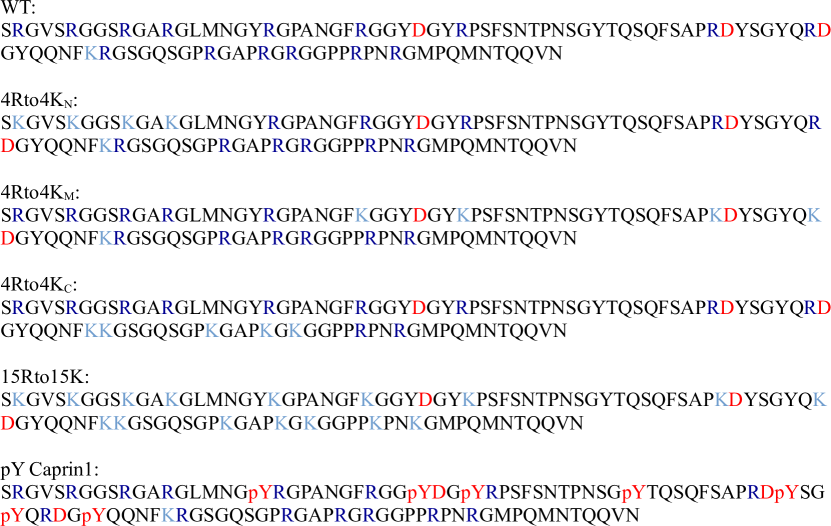
Fig. S1: Sequences of wildtype (WT) and variant Caprin1 IDR studied in this work. Positively charged arginine (R) and lysine (K) residues are shown, respectively, in dark and light blue, negatively charged aspartic acid (D) residues and phosphorylated tyrosines (pY) are shown in red. Other residues are in black.

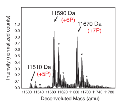
Fig. S2: Mass spectrometry analysis of pY-Caprin1. The graph plots deconvoluted mass (in atomic mass units, amu) on the horizontal axis against intensity (normalized counts) on the vertical axis. Peaks are observed at 11510 Da (+5 phosphate groups, +5P), 11590 Da (+6P), and 11670 Da (+7P). Asterisks mark the peaks of pY-Caprin1 with oxidized methionine residues.

Physical theories of Caprin1 and phosphorylated Caprin1 LLPSs as those of polyelectrolytes and polyampholytes
The 103-residue Caprin1 specified above is a highly charged IDR. It has 19 charged residues (Fig. 1a and Supplementary Fig. S1): 15 R, 1 K, and 3 aspartic acids (D); fraction of charged residues $=19/103=0.184$ and net charge per residue $=13/103=0.126$. With a substantial positive net charge, Caprin1’s phase behaviors are markedly different from those of polyampholytic IDRs with nearly zero net charge such as Ddx4 to which early sequence-specific LLPS theories were targeted.Nott15 ; linPRL ; linJML In this regard, Caprin1 behaves like chemically synthesized polyelectrolytesDobrynin2005 instead. In contrast, when most or all of the seven tyrosines (Y) in the Caprin1 IDR are phosphorylated, negative charges ($-2$ per phosphorylation) are added to the IDR, resulting in a near-neutral polyampholyte. Mass spectrometry indicates that the experimental sample of phosphorylated Caprin1 consists mainly of a mixture of IDRs with six or seven phosphorylations, with only a very small fraction of IDRs with five phosphorylations, and essentially no population with fewer than five phosphorylations (Supplementary Fig. S2). We refer to this sample as pY-Caprin1 in our presentation of experimental results below. For simplicity, we use only the Caprin1 IDR with all seven tyrosines phosphorylated to model the behavior of this highly phosphorylated experimental sample in our theoretical and computational formulations, partly to avoid the combinatoric complexity of sequences with five or six phosphorylations (which entail 21 and 7 possible different sequences, respectively, with unknown population fractions). Accordingly, since the charge on a phosphorylated tyrosine is expected to be $\approx-2$ at the experimental pH $=7.4$, $-2\times 7=-14$ charges are added to the Caprin1 IDR for our model pY-Caprin1 sequence, resulting in a near-neutral polyampholyte with a very small net charge per residue $=-1/103=-0.00971$ (Fig. 1b). Both the experimental pY-Caprin1 sample (net charge per residue $\approx\pm 1/103=\pm 0.00971$) and our model pY-Caprin1 are expected to exhibit phase properties similar to other polyampholytic IDRs.

Notably, sequence-specific RPA has been applied successfully to model electrostatic effects on the LLPSs of various polyampholytic IDR systems to obtain behaviorial trends consistent with experiments and explicit-chain simulations;linPRL ; linJML ; lin2017 ; njp2017 ; biochemrev ; SumanPNAS ; Wessen2021 but RPA is less appropriate for polyelectrolytes with large net charge per residue.Mahdi2000 ; Ermoshkin2003 ; Orkoulas2003 A major source of RPA’s differential effectiveness for polyampholytes and polyelectrolytes is its treatment of polymers as ideal Gaussian chains. This approximation is reasonable for polyampholytes but not for polyelectrolytes. While overall intrachain electrostatic effects in polyampholytes can be mild because of the polymers’ nearly zero net charge and thus entail only a minor perturbation on conformational statistics, repulsive electrostatics in polyelectrolytes with significant net charge is strong, leading to more rod-like conformations with statistics deviating significantly from that of Gaussian chains. Consequently, treating polyelectrolytes as Gaussian chains can lead to large errors in theoretical intrachain and interchain residue-residue (monomer-monomer) correlations, resulting in drastically overestimated LLPS propensities.MuthuMacro2017 Traditionally, theories for polyelectrolytes tackle their peculiar conformations by various renormalized blob constructs,Mahdi2000 ; Dobrynin2005 two-loop polymer field theory,Muthu1996 , modified thermodynamic perturbation theory,Budkov2015 and renormalized Gaussian fluctuation (RGF) theory,Shen2017 ; Shen2018 among others. As such, these formulations are mostly designed for homopolymers in which all residues (monomers) are identical, making it difficult to generalize them to biopolymers with heteropolymeric sequence patterns.

Here we present a novel theoretical analysis of Caprin1 phase behaviors using the recently developed renormalized-Gaussian random-phase approximation (rG-RPA) LLPS theorykings2020 that combines the idea of RGF theory and an approximation of charged heteropolymers as Gaussian chains with a sequence-charge-pattern-dependent effective (renormalized) Kuhn length.kings2015 As rG-RPA has been designed and verified to tackle polyeletrolyte conformations appropriately,kings2020 we apply it here to the polyelectrolytic Caprin1 IDR. Because rG-RPA allows for a smooth crossover between polyelectrolytic and polyampholytic systems, Caprin1 and pY-Caprin1 can now be analyzed in a universal theoretical formulation without invocation of ad hoc treatments for their different conformational statistics.

Phase properties predicted by rG-RPA theory for Caprin1 and pY-Caprin1 with monovalent counterions and salt are in agreement with experiment
Fig. 1c and d show that the salt- and temperature-dependent phase diagrams predicted by the rG-RPA free energy with an augmented Flory-Huggins (FH) mean-field $\chi(T)=\Delta h/T-\Delta s$ parameter for nonelectrostatic interactionslinPRL ; kings2020 in Caprin1 and pY-Caprin1 (this rG-RPA+FH formulation is described in Supplementary Information) are in reasonably good agreement with experimental dilute- and condensed-phase IDR concentrations at different temperatures (determined using bulk [Caprin1] $\approx 200$ $\mu$M). For Caprin1, the rG-RPA+FH results in Fig. 1c (color curves) indicate that (i) Caprin1 undergoes LLPS below 20^∘C with 100 mM NaCl, and that (ii) LLPS propensity, quantified by the upper critical solution temperature (UCST), increases with [NaCl] increasing from 100 mM to 300 mM and then 500 mM. These theoretical predictions are consistent with experimental data on Caprin1 (data-point symbols), including the observation that Caprin1 does not phase separate at room temperature without salt, ATP, RNA or other proteins, though Caprin1 LLPS can be triggered by adding WT and phosphorylated FMRP and/or RNA (bulk [Caprin1] $\gtrsim 10$ $\mu$M),julie2019 NaCl,LewisJACS2020 or ATP (bulk [Caprin1] $=400$ $\mu$M). LewisPNAS2021 The present theoretical trend is also in line with that predicted by other theories of polyelectrolyte phase behaviors.Shen2018 For pY-Caprin1, by comparison, Fig. 1d shows that rG-RPA+FH predicts decreasing LLPS propensity with increasing [NaCl] (color curves), consistent with experimental data (data-point symbols) as well as the expected salt dependence of LLPS of nearly neutral polyampholytic IDRs such as Ddx4.linPRL Interestingly, the decrease in some of the condensed-phase pY-Caprin1 concentrations with decreasing temperature (orange and green symbols for $\lesssim 20^{\circ}$C in Fig. 1d trending toward slightly lower [pY-Caprin1]) is suggestive of a lower critical solution temperature (LCST)biochemrev ; jeetainACS -like reduction of LLPS propensity at lower temperatures approaching $\sim 0^{\circ}$C.

Salt-IDR two-dimensional phase diagrams are instrumental for exploring broader phase properties
We now examine Caprin1 LLPS more closely for possible differences in salt concentration between the IDR-dilute and IDR-condensed phases, noting that the phase diagrams in Fig. 1c and d, though informative, are computed by a restricted application of rG-RPA that treats [Na⁺] as spatially uniform under the simplifying assumption that salt concentration is identical in the IDR-dilute and IDR-condensed phases. While this approximation is reasonable under certain circumstances,kings2020 it does not apply in general. Biologically, the difference in IDR-dilute- and IDR-condensed-phase salt concentration is of functional interest as a possible mechanism for selective enrichment or attenuation of certain salt species by biomolecular phase separation. Since the complete salt-protein phase behavior is accessible to theoretical modeling via rG-RPA, we now compute the two-dimensional salt-Caprin1 and salt-pY-Caprin1 phase diagrams at room temperature (300 K) by rG-RPA to assess this phase-dependent salt concentration difference (Fig. 2).

In accordance with the formulation outlined in Methods and detailed in Supplementary Information, “counterions” are defined here as the small ions that carry charges opposite in sign to that of the net charge of a given polymer (Caprin1 or pY-Caprin1), and “salt ions” are small ions that carry charges identical in sign to that of the polymer net charge. For the Caprin1/NaCl system, since Caprin1’s net charge is positive, Na⁺ is salt ion and Cl^- is counterion. Since the system as a whole is electrically neutral, the concentrations of polymer, counterions, and salt ions, denoted respectively as $\rho_{\rm p}$, $\rho_{\rm c}$, and $\rho_{\rm s}$, are constrained by the general relation

$$|Q|\rho_{\rm p}+z_{\rm s}\rho_{\rm s}=z_{\rm c}\rho_{\rm c}\;,$$ (1)

where $Q$ is the net charge of the polymer, $z_{\rm s}$ and $z_{\rm c}$ are, respectively, the valencies of salt ions and counterions. For Caprin1 and pY-Caprin1, $Q=+13$ and $-1$, respectively, and $(z_{\rm s},z_{\rm c})=(1,1)$, $(1,2)$, and $(2,4)$ are models for different small-ion species in the system. Specifically, in Fig. 2, we identify the $z_{\rm s}=1$ salt ion as Na⁺ (Fig. 2a–f) and the $z_{c}=1$ counterion as Cl^- (Fig. 2a–d), the $z_{\rm c}=2$ counterion as (ATP-Mg)^2- (Fig. 2g,h), the $z_{\rm s}=2$ salt ion as Mg²⁺ and the $z_{c}=4$ counterion as ATP^4- (Fig. 2i–l).

Behavioral trends of rG-RPA-predicted Na⁺-Caprin1 two-dimensional phase diagrams are consistent with experiment
Accordingly, the Caprin1-Na⁺ phase diagram at $T=300$ K computed using rG-RPA for the Caprin1-NaCl system in Fig. 2a ($z_{\rm s}=z_{\rm c}=1$) predicts that Caprin1 does not phase separate without salt (as highlighted by the zoom-in Fig. 2b), consistent with the aforementioned experimental observation, indicating that monovalent counterions alone (Cl^- in this case) are insufficient for Caprin1 LLPS. When the concentration of monovalent salt ion Na⁺ is increased, the system starts to phase separate at a small concentration of Na⁺ ($<0.1$ M), with phase separation propensity increasing until it reaches a plateau at [Na⁺] $\sim$1 M before decreasing at significantly higher [Na⁺] (Fig. 3a, blue-data points), in agreement with the results obtained by assuming a spatially uniform salt concentration in Fig. 1c that phase separation propensity increases monotonically with [NaCl] from 100 to 500 mM. Fig. 2a also predicts a reentrant dissolution of Caprin1 condensate at high [Na⁺]’s well above the physiological value. Our experimental measurement up to [Na⁺] $\approx 4.6$ M is consistent with this prediction (Fig.3a, blue data-points), as it indicates a significant decrease in LLPS propensity when [Na⁺] is increased above $\sim 2.5$ M, though the trend of gradually drecreasing LLPS propensity suggests that complete dissolution of condensed droplets is not likely to occur before NaCl reaches its saturation concentration of $\sim 6$ M when crystalline NaCl will precipitate from the aqueous solution and further increase in [Na⁺] becomes impossible. The negative tieline slopes in Fig. 2a,b mean that Na⁺ is predicted by rG-RPA to be partially excluded from the Caprin1 condensed phase. This “salt partitioning” phenomenon is most likely caused by Caprin1’s net positive charge and is consistent with published research on polyelectrolyte phase behavior with monovalent salt ions.Shen2018 ; Eisenberg1959 ; Moreira2001 ; Zhang2016 The predicted trend is consistent with our experiment showing significantly reduced concentrations of Na⁺ in the Caprin1 condensed phase in comparison with the Caprin1-dilute phase (Table 1), although the larger experimentally observed reduction of [Na⁺] in the Caprin1 condensed droplet relative to our theoretical prediction is a quantitative detail that remains to be elucidated. In contrast, for the near-neutral, very slightly negative pY-Caprin1 (Fig. 2c,d), phase separation can occur at [Na⁺] $\approx 0$, and the positive slopes of the tielines indicate that the concentration of Na⁺ is generally higher in the condensed phase than in the dilute phase. Consistent with Fig. 1d, Fig. 2c shows that LLPS propensity decreases with increasing [Na⁺] for any given [pY-Caprin1].

rG-RPA-predicted salt-IDR two-dimensional phase diagrams underscore different effects of monovalent and divalent counterions on LLPS
Interestingly, a different salt dependence of Caprin1 LLPS is observed theoretically when the monovalent salt ion Na⁺ remains unchanged but the monovalent counterion Cl^- in Fig. 2a–d is replaced by a divalent $z_{c}=2$ anion modeling the (ATP-Mg)^2- ionic complex under the assumption that the ATP^4- and Mg²⁺ do not dissociate in solution. The rG-RPA phase diagrams at room temperature for this system (Fig. 2e–h) predict that as long as the divalent counterions are present (Fig. 2g,h), Caprin1 can undergo LLPS without the monvalent salt (Na⁺) ions (phase-separated regime extend to [Na⁺] $=0$ in Fig. 2e,f). A likely reason for this difference is that there is a configurational entropic cost of concentrating the monovalent Cl^- counterions in the Caprin1 condensed phase. Apparently, when [Cl^-] is just sufficient to balance the net positive charge of Caprin1 (i.e., when [Na⁺] = 0), this entropic cost cannot be overcome for Caprin1 LLPS to occur. The entropic cost will be lessened (and thus more favorable to Caprin1 LLPS) when there are more Cl^- ions beyond what is necessary to balance the net positive charge of Caprin1, corresponding to a situation with nonzero [Na⁺] from the added NaCl to supply the additional Cl^- ions. In comparison, when the counterion is divalent [(ATP-Mg)^2- in our case], the number of counterions needed for balancing the positive net charge of Caprin1 is half of that when the counterion is monovalent. It follows that the entropic cost of concentrating the divalent counterion in the Caprin1-condensed phase is less and consequently, at least in the present situation, no added salt is needed for Caprin1 LLPS.

Aside from this basic contrast between movalent and divalent counterions in their effects on the LLPS of the polyelectrolytic Caprin1, there are additional notable rG-RPA-predicted differences: (i) The maximum condensed-phase Caprin1 concentration at low [Na⁺] is much higher with divalent counterions ([Caprin1] $\sim 750$ mM, Fig. 2e,f) than with monovalent counterions ([Caprin1] $\sim 400$ mM, Fig. 2a.b). (ii) The [Na⁺] above which increasing [Na⁺] decreases Caprin1 LLPS toward reentrance of the homogeneous phase (corresponding to the [Na⁺] at the maximum phase-separated Caprin1 concentration) is much lower with divalent counterions ([Na⁺] $\sim 0.1$ M in Fig. 2e,f) than with monovalent counterions ([Na⁺] $\sim 1$ M in Fig. 2a,b). (iii) The rG-RPA-predicted differential [Na⁺] between the Caprin1-dilute and Caprin1-condensed phases as indicated by the tielines exhibit different trends for divalent and monovalent counterions. Although [Na⁺] is depleted in the Caprin1-condensed phase in both systems when the overall [Na⁺] is high (negative tieline slopes for [Na⁺]$\gtrsim$ 2 M in Fig. 2a,e), there is a regime with relatively lower overall [Na⁺] in which Na⁺ concentration is slightly higher in the Caprin1-condensed than in the Caprin1-dilute phase with divalent counterions but not with monovalent counterions as indicated by the slightly positive slopes of the tielines for [Na⁺]$\lesssim$ 2 M in Fig.2e,f. This rG-RPA result suggests that, in the intracellular environment where [Na⁺]=150$\sim$170 mM, monovalent positively charged salt ions such as Na⁺ can be attracted, somewhat counterintuitively, into biomolecular condensates formed from positively charged polyelectrolytic IDRs in the presence of divalent counterions.

rG-RPA predictions are consistent with experimental ATP-Mg-dependent Caprin1 reentranct phase behaviors
We next consider a case in which both the salt ions and counterions are multivalent, namely the $z_{\rm s}=2$, $z_{\rm c}=4$ case serving as a model of the ATP-Mg complex dissociated completely in solution into Mg²⁺ salt ions and ATP^4- counterions. For this system, the rG-RPA results in Fig. 2i–l predict that Caprin1 can undergo LLPS with the ATP^4- counterions (Fig. 2k,l) in the absence of the Mg²⁺ salt ions (i.e., the phase-separated regime includes the horizontal axes in Fig. 2i,j), likely for a reason similar to that mentioned above for the case with a divalent counterion because the loss of configurational entropy of concentrating tetravalent counterions in the Caprin1-condensed phase is even less than that of concentrating divalent counterions. Here, the tetravalent counterion increases the maximum condensed-phase Caprin1 concentration to $\gtrsim$1200 mM beyond the aforementioned $\sim 750$ mM and $\sim 400$ mM, respectively, for divalent and monovalent counterions. The [Mg²⁺] above which increasing Mg⁺ concentration decreases Caprin1 LLPS toward reentrance of the homogeneous phase (i.e., the [Mg²⁺] at the maximum phase-separated Caprin1 concentration in Fig. 2i,j) is $\sim$400 mM, which is intermediate between the corresponding Na⁺ concentrations of $\sim 0.1$ and $1$ M with $(z_{\rm s},z_{\rm c})=(1,2)$ and $(1,1$), respectively, for divalent and monovalent counterions. Notably, all the tielines for Mg²⁺ and ATP^4- in the phase-separated regime in Fig. 2i–l have significantly positive slopes, except in an extremely high-salt region with [Mg²⁺]$>8$M, indicating that ATP-Mg concentration is almost always substantially enhanced in the Caprin1-condensed phase than in the Caprin1-dilute phase. Although polymer field theories tend to overestimate LLPS propensity and thus condensed-phase concentrations because they do not account for ion condensationShen2017 —which can be severe for small ions with more than $\pm 1$ charge valencies, the qualitative and semi-quantitative trends predicted here by rG-RPA should be reliable. Indeed, consistent with our rG-RPA results, experimental measurements indicate reentrant phase behavior of Caprin1 as ATP-Mg concentration is varied, with LLPS propensity enhanced initially by ATP-Mg at low [(ATP-Mg)^2-] then suppressed by high [(ATP-Mg)^2-] (Fig. 3a, red data-points, and Fig. 3b), and that both [Mg²⁺] and [ATP^4-] are significantly enhanced (by a factor of $\sim 5$–$60$ for overall [(ATP-Mg)^2-] = 3–30 mM) in the Caprin1-condensed phase relative to the Caprin1-dilute phase (Table 2).

Coarse-grained MD with explicit small ions is useful for investigating subtle salt dependence in biomolecular LLPS
To gain deeper insights into the molecular basis of the salt-dependent experimental and rG-RPA-predicted reentrant phase behavior of Caprin1, we extend the widely-utilized coarse-grained explicit-chain MD model for biomolecular condensatesSumanPNAS ; dignon18 ; panag2017 to include explicit small cations and anions in the simulation of Caprin1 phase properties. Instead of approximating the effects of salt by Debye screening, each Na⁺ or Cl^- is modeled as a charged bead with excluded volume in our attempt to capture the experimental reentrance trend (Methods). For computational efficiency, we neglect for now many possible subtle solvation effects that can arise from the directional hydrogen bonds among water molecules (see, e.g., ref. (122)) by treating other aspects of the aqueous solvent implicitly as in most, though not all,Wessen2021 ; MiMB2023 applications of the methodology.dignon18 Several interaction schemes were devised and utilized in recent coarse-grained MD simulations of biomolecular LLPS (see, e.g., refs. (91; 98; 100; 123; 124; 125; 104)). Because this study is primarily interested in general principles rather than quantitative details of the phase behaviors of Caprin1 and its ariginine-to-lysine (RtoK) mutants, as a first investigative step we adopt the Kim-Hummer (KH) energiesKH for pairwise amino acid interactions. The KH scheme was derived from classic statistical analyses of folded protein structures in the Protein Data Bank by Miyazawa and Jernigan.MJ96 It can largely capture the different experimental effects of arginine versus lysine on LLPS.SumanPNAS Nonetheless, it will be instructive to compare the results predicted by different interaction schemes in future studies.

Explicit-ion MD rationalizes experimentally observed [NaCl]-dependent Caprin1 reentrant phase behaviors and depletion of Na⁺ in Caprin1 condensate
Consistent with experimental data (Fig. 3) and our rG-RPA prediction in Fig. 1c,d, our explicit-ion coarse-grained MD results show [NaCl]-dependent reentrant phase behavior for Caprin1 (non-monotonic trend indicated by the grey arrow in Fig. 4a) but not for pY-Caprin1 (monotonic trend indicated by the grey arrow in Fig. 4b). In other words, the critical temperature $T_{\rm cr}$, which is defined as the maximum temperature (UCST) of a given phase diagram (binodal, or coexistence curve), increases then decreases with addition of NaCl for Caprin1 but $T_{\rm cr}$ always decreases with increasing [NaCl] for pY-Caprin1. Moreover, consistent with the rG-RPA-predicted tieline slopes in Fig. 1a–d (negative slopes for Caprin1 and positive slopes for pY-Caprin1), explicit-ion coarse-grained MD predicts that Na⁺ is slightly depleted in the condensed droplet of Caprin1 relative to the Caprin1-dilute phase (Fig. 4c) but is enhanced in the pY-Caprin1 droplet (Fig. 4d). As noted above, both of these trends are consistent with experiment (Fig. 3a, blue data-points; and Table 1). Note that model temperatures in Fig. 4a,b and subsequent MD results are given in units of the MD-simulated $T_{\rm cr}$ of wildtype (WT) Caprin1 at [NaCl] $=0$, denoted here as $T^{0}_{\rm cr}$. It follows that for systems with higher or lower LLPS propensities than WT Caprin1 at zero [NaCl], their $T_{\rm cr}$’s are, respectively, higher or lower than $T^{0}_{\rm cr}$, i.e., $T_{\rm cr}/T^{0}_{\rm cr}>1$ or $T_{\rm cr}/T^{0}_{\rm cr}<1$.

Fig. 4c shows further that in the Caprin1-condensed phase, an enhancement of [Cl^-] is concomitant with a depletion of [Na⁺]. This differential trend is further illustrated in Fig. 5a-d showing, for the entire simulation box (Fig. 5a), the spatial positions of the Caprin1 IDR (Fig. 5b) as well as those of the small ions Na⁺ (Fig. 5c) and Cl^- (Fig. 5d) in separate representations of the same MD snapshot. Notably, a similar trend attributed to IDR charge effects has been observed in explicit-water, explicit-ion MD simulations in the presence of a preformed condensate of the N-terminal RGG domain of LAF-1 with a positive net charge.Zhengetal-ions2020 For the present polycationic Caprin1, we now utilize the spatial/structural information of the coarse-grained MD trajectories to take a closer look at a possible molecular basis for Cl^-’s facilitation of Caprin1 LLPS. Consistent with an early analysis based on explicit-ion lattice-model simulations by Panagiotopoulos and coworkers,Orkoulas2003 the zoom-in views in Fig. 5e,f suggest that, as counterion, Cl^-’s can serve to coordinate two positively charged arginine residues and thereby stabilizing indirect counterion-bridged interchain contacts among Caprin1 molecules to promote Caprin1 LLPS.

Explicit-ion MD rationalizes [NaCl]-dependent phase properties of arginine-lysine mutants of Caprin1
In addition to WT Caprin1, a similar trend of [NaCl]-dependent LLPS propensities were observed experimentally for three of the four Caprin1 variants involving RtoK substitutions studied recently, though the computationally-predicted reentrant dissolution is not observed experimentally at the highest [NaCl] studied.LewisJACS2020 The amino acid sequences of these variants, termed 15Rto15K, 4Rto4K_N, 4Rto4K_M, and 4Rto4K_C (provided in Supplementary Fig. S1), involve 15 or 4 RtoK substitutions.LewisJACS2020 Coarse-grained MD is readily applicable to studying variations in LLPS properties among RtoK mutants.SumanPNAS In contrast, since RtoK substitutions do not change the sequence charge pattern of any given sequence, rG-RPA theory as formulated above does not account for their effects on LLPS, though polymer field theory can be extended to incorporate such effects in more sophisticated formulations.WessenJPCB2022

The phase diagrams in Fig. 6 obtained from explicit-ion coarse-grained MD exhibit reentrant phase behaviors for all three 4Rto4K Caprin1 variants. While these simulation results are consistent with experimental data showing phase separation of these 4Rto4K variants commencing at different nonzero NaCl concentrations (see below), the simulated reentrant dissolution is not observed experimentally, probably because the simulated [NaCl] needed for reentrant dissolution is beyond the experimentally investigated or physically possible range of salt concentration. It should also be noted that although reentrant phase behaviors are also seen in our simulation for the 15Rto15K variant, its much lower LLPS propensity (as quantified by a much lower theoretical UCST) is consistent with no experimental observation of LLPS for this variant,LewisJACS2020 as will be explained below. Since our main goal here is to ascertain whether simple electrostatic interactions among the small Na⁺, Cl^- ions and Caprin1 or its variants is sufficient, in principle, to provide the essential physical features capable of capturing the experimental trend, we do not attempt to fine-tune the energetic parameters in the explicit-ion coarse-grained MD models to achieve a quantitative match between MD simulation and experiment. For instance, when the phase behaviors of the five Caprin1 sequences are monitored experimentally (Fig. 9 of ref. (86) and Fig. 3a of this article), only WT exhibits a clear trend toward reentrant dissolution of condensed droplets (with a LLPS propensity plateau at [NaCl] $\approx 1.55$–$2.5$ M, Fig. 3a, blue data-points), whereas the LLPS of 4Rto4K_M and 4Rto4K_C commences at [NaCl] $\approx 1.3$ M, LLPS propensity then increases with [NaCl] (a trend consistent with the increasing LLPS propensity at low [NaCl]’s predicted by MD in Fig. 6b,c), but no sign of reentrant dissolution is seen up to the maximum [NaCl] = 2 M investigated experimentally for the RtoK variants (Fig. 9B of ref. (86)). In contrast, the phase diagrams simulated by coarse-grained MD in Fig. 6 show a maximum LLPS propensity (highest $T_{\rm cr}$) at [NaCl] $\approx 0.5$ M. This qualitative agreement with quantitative mismatch suggests that real Caprin1 LLPS is somewhat less sensitive to small monovalent ions than that stipulated by the present MD model. This question should be tackled in future studies by more in-depth considerations of the model interaction scheme, including but not limited to exploration of refined small-ion-protein interaction parameters, possible physical features captured by alternate pairwise amino acid interaction energies,dignon18 ; SumanPNAS ; Mpipi ; Urry-Mittal ; FB ; Kresten ; WessenJPCB2022 and their temperature dependence.jeetainACS ; Roland2019

Limitations of our MD model notwithstanding, the sequence-dependent trend showcased in our MD-simulated phase diagrams agrees largely with experiment. LLPS propensities as measured by the MD-simulated $T_{\rm cr}$’s in Fig. 6 follow the rank order of WT $>$ 4Rto4K_M $>$ 4RtoK_N $\approx$ 4Rto4K_C $>$ 15Rto15K. This order is essentially identical to that measured experimentally, viz., WT $>$ 4Rto4K_M $>$ 4RtoK_C $>$ 4Rto4K_N $>$ 15Rto15K (Fig. 9B of ref. (86)). The degree to which the differences in simulated LLPS propensity among these Caprin1 variants are affected by how interactions involving K and R are treated differently by the model potential functionSumanPNAS ; Mpipi should be further explored. In comparing coarse-grained implicit-solvent MD-simulated LLPS data and experimental phase behaviors, one recognizes logically that a low simulated $T_{\rm cr}$ may mean no experimentally observed LLPS at all because the theoretical $T_{\rm cr}$ can be below the freezing temperature of the aqueous solvent in the real system.linPRL ; jacob2017 In this regard, the MD-simulated results in Fig. 6a showing that even the highest $T_{\rm cr}$ for 15Rto15K (at [NaCl] = 480 mM) is essentially at the same level as $T^{0}_{\rm cr}$ for WT at [NaCl] = 0 ($T_{\rm cr}/T^{0}_{\rm cr}\approx 1$) is consistent with the experimental observations of no LLPS for 15Rto15K up to at least [NaCl] = 2 M as well as no LLPS for WT Caprin1 at [NaCl] = 0 (Fig. 9B,C of ref. (86)). Taken together, the above favorable comparisons between coarse-grained MD and experiment underscore a major role of electrostatics in the observed salt-dependent phase properties of WT and RtoK variants of Caprin1.

Field-theoretic simulation is an efficient tool for studying multiple-component phase properties
We next turn to modeling of Caprin1 or pY-Caprin1 LLPS modulated by both ATP-Mg and NaCl. This task entails more complex theoretical constructs, which should provide more realistic representations and thus offer predictions for subtler behaviors of the corresponding experimental systems than the above rG-RPA or coarse-grained MD models that contain only a single pair of small ions. Because tackling such many-component LLPS systems using either rG-RPA or explicit-ion MD is numerically challenging currently, we adopt the complementary field-theoretic simulation (FTS)Fredrickson2006 approach as an initial step in this aspect of our expanded investigation. FTS is based on complex Langevin dynamics,Parisi1983 ; Klauder1983 which is related to an earlier formulation for stochastic quantization of field theoryParisiWu1981 ; MBH_Ghostfree and has been applied extensively to study polymer solutions.Fredrickson2002 ; Fredrickson2006 It is based on the mathematical principle that thermal (Boltzmann) averages of a real-space system can be computed as asymptotic fictitious-time averages of the field operators corresponding to the thermodynamic observable of interest.Parisi1983 ; Klauder1983 Recently, the approach has provided important insights into the impact of sequence-dependent LLPS effects on biomolecular condensates containing charged IDRs.joanJPCL2019 ; joanElife ; Pal2021 ; WessenJPCB2022 ; MiMB2023 For a given system, the basic starting point of FTS is identical to that of rG-RPA. FTS invokes no RPA and thus enjoys a clear advantage over rG-RPA in this regard, though it is still limited by the lattice size used for simulation and its flexibility in treating excluded volume.Pal2021 Here we apply the protocol detailed in refs. (106; 101) and outlined here in Methods and Supplementary Material.

A simple model of ATP-Mg for field-theoretic simulation
In order to utilize FTS for exploring general physical principles, we adopt a 6-bead polymeric representation of (ATP-Mg)^2- (Fig. 7a) in which four negative and two positive charges serve to model ATP^4- and Mg²⁺ respectively. Modeling (ATP-Mg)^2- as a short charged polymer enables application of existing FTS formulations for multiple charge sequences to systems with IDRs and (ATP-Mg)^2-. While the model in Fig. 7a does not capture structural details, its charge distribution does correspond roughly to that of the chemical structure of (ATP-Mg)^2-. In developing FTS models involving IDR, (ATP-Mg)^2-, and NaCl, we first assume for simplicity that (ATP-Mg)^2- does not dissociate and consider FTS systems for the Caprin1 or pY-Caprin1 IDR consisting of any given bulk concentrations of IDR and (ATP-Mg)^2- wherein all positive and negative charges on the IDR and (ATP-Mg)^2- are balanced, respectively, by Cl^- and Na⁺ (Fig. 7a) to maintain overall electric neutrality (see legend for Fig. 7).

Phase behaviors can be probed by field-theoretic density correlation functions
As discussed previously, LLPS propensity of FTS systems can be monitored using correlation functions.Pal2021 Here the formulation in ref. (106) is applied to our Caprin1/pY-Caprin1 + ATP-Mg + NaCl systems to obtain intra-species self-correlation functions $G_{\rm pp}(r)$ for the IDRs (Fig. 7b,c) as well as inter-species cross-correlation functions $G_{\rm pq}(r)$ between the IDR and (ATP-Mg)^2- or NaCl (Fig. 7d,e) at three different bulk (ATP-Mg)^2- concentrations of $10^{-4}b^{-3}$, $0.03b^{-3}$, and $0.5b^{-3}$, where the polymer Kuhn length $b$ may be taken as the peptide virtual bond length $\approx 3.8$Å  (see Methods and Supplementary Information for definitions and further discussion). The correlation functions in Fig. 7 for Caprin1 (left column) and pY-Caprin1 (right column) are normalized by bulk density $\rho^{0}_{\rm p}$ of the IDR and the bulk densities $\rho^{0}_{\rm q}$ for (ATP-Mg)^2- or Na⁺ or Cl^-. Density of any species is defined here as the bead density of the species in units of $b^{-3}$. Phase separation of the IDR is signaled by its normalized self-correlation function in Fig. 7b,c dropping below the baseline $G_{\rm pp}(r)/(\rho^{0}_{\rm p})^{2}=1$ (marked by black horizontal dashed lines) at large distance $r$ because this feature is sufficient for inferring that there is at least a spatial region with IDR below the bulk concentration. Since the total amount of IDR in the system is a given, this is only possible if IDR concentration is above the bulk concentration in at least another spatial region, i.e., in one or more relatively condensed droplets. In other words, $G_{\rm pp}(r)/(\rho^{0}_{\rm p})^{2}<1$ for large $r$ indicates definitely that IDR concentration is heterogeneous in the system with relatively IDR-condensed and IDR-dilute regions, i.e., the system is phase separated. In general, $G_{\rm pp}(r)/(\rho^{0}_{\rm p})^{2}$ is expected to increase for small $r$ because IDR chain connectivity tends to facilitate correlation of residue positions among residues local in the chain sequence. On top of that, propensity to phase separate may be quantified by the small-$r$ values of the IDR self-correlation function because a higher value of $G_{\rm pp}(r)/(\rho^{0}_{\rm p})^{2}$ then indicates a higher tendency for different chains to associate and hence a higher LLPS propensity.Pal2021

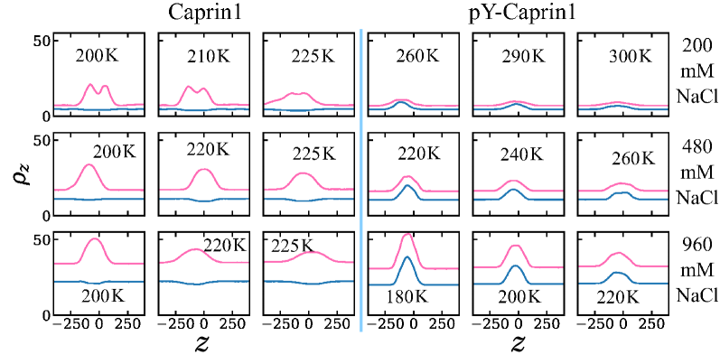
Fig. S3: Explicit-ion coarse-grained molecular dynamics simulation of salt and counterion density profiles in protein-dilute and protein-condensed phases of Caprin1 and pY-Caprin1. Density $\rho_{z}$ profiles for Na⁺ (blue) and Cl^- (red) for the Caprin1 (three left columns) and pY-Caprin1 (three right columns) systems are shown as in Fig. 4e,f of the maintext. Regions with elevated [Cl^-] here coincide with positions of the condensed protein droplets. Overall [NaCl] values used for the simulations are provided on the right.

Field-theoretic simulation rationalizes [ATP-Mg]-modulated Caprin1 reentrant phase behaviors and their colocalization in the Caprin1-condensed phase
The FTS-computed self-correlation functions in Fig. 7 indicates reentrant LLPS behavior—i.e., nonmonotonic variaion in LLPS propensity—with respect to [(ATP-Mg)^2-] for Caprin1 but not for pY-Caprin1: When [(ATP-Mg)^2-]/$b^{-3}$ varies from $10^{-4}$ to $0.03$ to $0.5$, small-$r$ values of the Caprin1-Caprin1 $G_{\rm pp}(r)$ in Fig. 7b initially increase then decrease, whereas the corresponding small-$r$ values of the pY-Caprin1-pY-Caprin1 $G_{\rm pp}(r)$ in Fig. 7c decrease monotonically. These trends are consistent with the above rG-RPA results in Fig. 2g,h,k,l and the experimental data in Fig. 3. The inter-species cross-correlation functions in Fig. 7d,e show further that when a Caprin1 or pY-Caprin1 condensed phase is present at [(ATP-Mg)^2-] = 0.03$b^{-3}$ (as indicated by the above-discussed large-$r$ behaviors of the corresponding $G_{\rm pp}(r)/(\rho^{0}_{\rm p})^{2}$ functions in Fig. 7b,c), (ATP-Mg)^2- is colocalized with Caprin1 or pY-Caprin1 (high value of $G_{\rm pq}/\rho^{0}_{\rm p}\rho^{0}_{\rm q}$ for small $r$) in the IDR-condensed droplet. By comparison, the variation of Na⁺ and Cl^- concentration within versus outside the IDR droplet is significantly weaker. For Caprin1, Cl^- is enhanced over Na⁺ in the Caprin1 condensed phase (small-$r$ $G_{\rm pq}/\rho^{0}_{\rm p}\rho^{0}_{\rm q}$ of the former larger than the latter in Fig. 7d), but the reverse is seen for the pY-Caprin1 condensed phase (Fig. 7e). This FTS-predicted difference is consistent with the coarse-grained MD results in Fig. 4c,d and Supplementary Fig. S3; and it most likely arises from the positive net charge on Caprin1 and the smaller negative net charge on pY-Caprin1.

Field-theoretic simulation rationalizes experimentally observed residue-specific binding of Caprin1 with ATP-Mg
The propensities for (ATP-Mg)^2-, Na⁺, and Cl^- to associate with each residue $i$ along the Caprin1 IDR sequence ($i=1,2,\dots,103$) in our FTS model are provided by the residue-specific integrated correlation ${\cal G}^{(i)}_{\rm pq}/\rho^{0}_{{\rm p},i}\rho^{0}_{\rm q}$ in Fig. 7f, which can be calculated efficiently using the FTS formulation. Because each ${\cal G}^{(i)}_{\rm pq}$ quantity is computed by integrating the corresponding correlation function $G^{(i)}_{\rm pq}(r)$ from $r=0$ to a relative short cutoff distance $r=r_{\rm contact}$ (in units of $b^{3}$), it measures a relative contact frequency for the IDR residue $i$ and ionic species q to be in spatial proximity (Methods and Supplementary Information). Notably, the residue-position-dependent integrated correlation for (ATP-Mg)^2- varies significantly, exhibiting much larger values near the N-terminal and a little before the C-terminal but weaker correlation elsewhere (Fig. 7f, red symbols). The two regions of high integrated correlation (i.e., favorable association) coincide with regions with high sequence concentration of positively charged residues. This FTS prediction is remarkably similar to the experimental NMR finding that binding between (ATP-Mg)^2- and Caprin1 occurs strongly at the arginine-rich N- and C-terminal regions, as indicated by the volume ratio $V/V_{0}$ data in Fig. 1C of ref. (87) that quantifies the ratio of peaks in NMR spectra in the presence and absence of trace amounts of ATP-Mn. For comparison with the FTS results, this set of experimental data is replotted as $1-V/V_{0}$ in Fig. 7f (grey symbols, right vertical axis) to illustrate the similarity in experimental and theoretical trends because $1-V/V_{0}$ is expected to trend with contact frequency. Corresponding FTS results for Na⁺ and Cl^- in Fig. 7f exhibit much less residue-position-dependent variation, with Cl^- displaying only slightly enhanced association in the same arginine-rich regions, and Na⁺ showing even less variation, presumably because the positive charges on Caprin1 are already essentially neuralized by the locally associated (ATP-Mg)^2- or Cl^- ions. The theory-experiment agreement in Fig. 7f regarding ATP-Caprin1 interactions indicates once again that electrostatics is an important driving force underlying many aspects of experimentally observed Caprin1–(ATP-Mg)^2- association. Indeed, this point is further underscored by a reasonably good agreement between the predicted magnitudes of effective Caprin1 residue-specific electrostatic potentials computed in FTS via potentials of mean force of test charges and the experimental NMR-determined values of residue-specific near-surface electrostatic potential $\phi_{\rm ENS}$ in ref. (88). Details of this more direct comparison between theory and experiment are provided in Supplementary Information (Fig. S4).

Field-theoretic simulation snapshots of [ATP-Mg]-modulated reentrant phase behaviors and Caprin1-ATP-Mg colocalization
The above FTS-predicted trends of Caprin1 versus pY-Caprin1 LLPS modulated by (ATP-Mg)^2- are further illustrated in Fig. 8 by snapshots of spatial distribution of the real part of the fields for various molecular and ionic components in the FTS formulation. Such field snapshots are generally useful for visualization and heuristic understanding of FTS-predicted phase behaviors,joanJPCL2019 ; Pal2021 ; WessenJPCB2022 including subtler aspects of spatial arrangements exemplified by recent applications to study patterns of subcompartmentalization entailing either co-mixing or demixing in multiple-component LLPS that are verifable by explicit-chain MD.Pal2021 ; WessenJPCB2022 For the present study of Caprin1 and pY-Caprin1, the [(ATP-Mg)^2-]-dependent trends deduced from the correlation functions in Fig. 7 are buttressed by the representative snapshots in Fig. 8: As the bead density of (ATP-Mg)^2- is increased from $10^{-4}b^{-3}$ to $0.03b^{-3}$ to $0.5b^{-3}$, the spatial distribution of Caprin1 evolves from an initially dispersed state to a concentrated droplet to a (reentrant) dispersed state again (Fig. 8a), whereas the initial dense pY-Caprin1 droplet becomes increasingly dispersed monotonically (Fig. 8b). Colocalization of (ATP-Mg)^2- with both the condensed Caprin1 (Fig. 8c) and pY-Caprin1 (Fig. 8d) droplets is clearly visible at [(ATP-Mg)^2-] $=0.03b^{-3}$, though the degree of colocalization is appreciably higher for Caprin1 than for pY-Caprin1. This predicted difference, which is likely caused by the positive net charge of Caprin1 being more attractive to (ATP-Mg)^2- than the slightly net negative charge of pY-Caprin1, remains to be further explored by theory and experiment. By comparison, variations in Na⁺ and Cl^- distribution between Caprin1/pY-Caprin1 dilute and condensed phase are not so discernible in their snapshots in Fig. 8e–h, which is expected from the small differences in the corresponding FTS correlation functions (Fig. 7d,e).

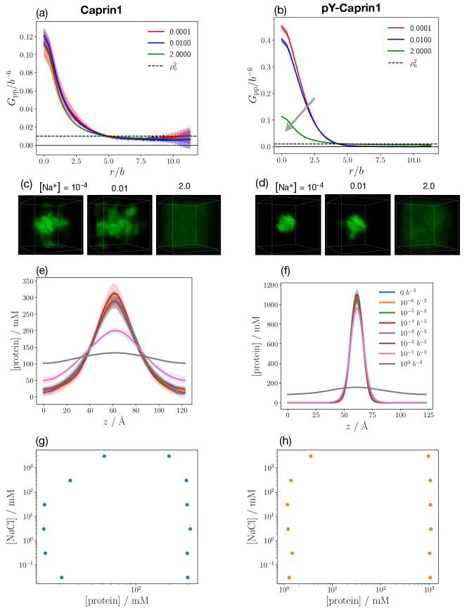
Fig. S5: FTS models for Caprin1 and pY-Caprin1 with only Na⁺ and Cl^- but no ATP-Mg. (a,b) Protein-protein correlation functions [Eq. (11) of maintext] for Caprin1 (a) and pY-Caprin1 (b) at three different [Na⁺], color coded in units of $b^{-3}$ as provided. In each figure, the baseline value of protein-protein correlation function $(\rho^{0}_{\rm p})^{2}$ (where $\rho^{0}_{\rm p}$ is overall protein concentration) is marked by the horizontal dashed line. Phase separation is indicated by large-$r$ correlation function values falling below this baseline. The grey arrow in (b) marks the direction of increasing [Na⁺]. (c,d) Field snapshots for the Caprin1 (c) and pY-Caprin1 (d) systems at different Na⁺ concentrations. The above results are obtained at Bjerrum length $l_{\rm B}=7b$. (e–h) Results from an alternate FTS model using an elongated simulation box similar to that utilized for coarse-grained molecular dynamics. (e,f) Protein concentration profiles computed at different NaCl concentrations for Caprin1 (e) and pY-Caprin1 (f) [color code for density profiles provided in (f)]. (g,h) salt-protein phase diagrams obtained from the concentration profiles in (e,f) for Caprin1 (g) and pY-Caprin1 (h). Details of the models are provided in Supplementary Methods.

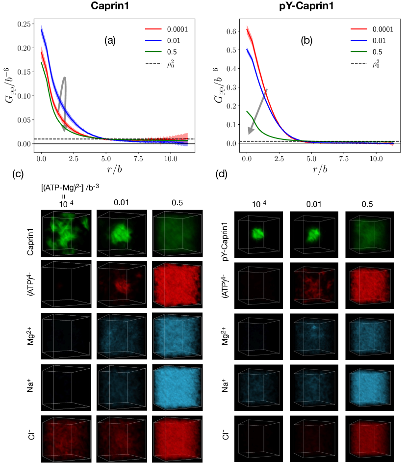
Fig. S7: Alternate FTS models for Caprin1 or pY-Caprin1 with ATP^4-, Mg²⁺, Na⁺ and Cl^-, wherein (ATP-Mg)^2- is assumed to be fully dissociated. Results are obtained for $l_{\rm B}=7b$ and presented in the same style as that in Fig. 7b,c and Fig. 8 of the maintext as well as Supplmentary Fig. S6. Details of the models are provided in Supplementary Methods.

Robustness of general trends predicted by field-theoretic simulation
In addition to the above comparison among FTS, rG-RPA and MD, we have further evaluated the robustness of the FTS predictions in Figs. 7 and 8 by studying the following pertinent FTS systems: (i) FTS models for Caprin1 or pY-Caprin1 with only Na⁺ and Cl^- but no (ATP-Mg)^2-. Consistent with rG-RPA and explicit-MD, these FTS models show reentrant behavior—albeit subtle—for Caprin1 but not for pY-Caprin1 (Supplementary Fig. S5). (ii) FTS model for Caprin1 with (ATP-Mg)^2- and either Na⁺ or Cl^- (but not both) to maintain overall charge neutrality; and FTS model for pY-Caprin1 with (ATP-Mg)^2-, and Na⁺ as counterion but no Cl^- (Supplementary Fig. S6). As assumed in Figs. 7 and 8, the (ATP-Mg)^2- in these models does not dissociate in solution. (iii) FTS models for Caprin1 or pY-Caprin1 with ATP^4-, Mg²⁺, Na⁺ and Cl^- (Supplementary Fig. S7). Unlike Figs. 7 and 8 and (ii), these models assume (ATP-Mg)^2- to be fully dissociated in solution. Despite the variation in assumptions between the FTS models in Figs.7 and 8 and these two alternate FTS models, the results in Supplementary Figs. S6 and S7 consistently show reentrant behavior for Caprin1 but not pY-Caprin1 as well as colocalization of ATP with condensed Caprin1 droplets, suggesting strongly that these features are general consequences of the basic electrostatic interactions of Caprin1/pY-Caprin1 + ATP-Mg + NaCl systems.

Discussion

Viewing our results from the above approaches of rG-RPA,kings2020 explicit-ion coarse-grained MD, and FTSjoanJPCL2019 ; MiMB2023 as a whole, one sees that salt-dependent reentrant phase behaviors are consistently predicted for Caprin1—manifested by an initial enhancement of LLPS at low salt with increasing salt followed by gradual dissolution of the condensed phase at high salt, whereas LLPS propensity of phosphorylated pY-Caprin1 is predicted to decrease monotonically with increasing salt (Figs. 2, 4, 7, and 8). This effect applies to small monovalent salt ions exemplified by Na⁺ and Cl^- as well as to our electrostatics-based models of (ATP-Mg)^2- or ATP^4-, with ATP notably exhibiting a significant colocalization with the Caprin1 condensed phase (Figs. 2g,h,k,l and 8c). These predicted trends are in broad agreement with experimental measurements. Because the predictions originate primarily from the electrostatic interactions in our theoretical formulations, the noted theory-experiment agreements—including a remarkable one regarding residue-specific ATP binding (Fig. 7f)—suggest strongly that electrostatics is a major driving force for these NaCl- and ATP-related but hydrolysis-independent behaviors in real Caprin1 systems.

Related studies of electrostatic effects on biomolecular condensates
The theoretical trends predicted here for Caprin1 and pY-Caprin1 are largely in agreement with recent computational studies on the differential concentrations of salt in the dilute versus condensed phaseZhengetal-ions2020 and salt-dependent reentrant behaviorsKnowlesNatComm2021 of other biomolecular condensates. As mentioned above, explicit-water, explicit-ion atomic simulations in the presence of a preformed condensate of the N-terminal RGG domain of LAF-1 with a net charge of $+4$ produce enhanced Cl^- and depleted Na⁺ in the IDR-condensed phase,Zhengetal-ions2020 consistent with our implicit-water, explicit-ion MD result in Fig. 4c for Caprin1 with net charge $+13$ (Fig. 4c). By comparison, corresponding simulations in the presence of a preformed condensate of the low complexity domain of FUS with a net charge of $-2$ produce a significant depletion of Cl^- and a minor depletion of Na⁺ in the IDR-condensed phase,Zhengetal-ions2020 which is opposite to the trend seen here for pY-Caprin1 with net charge $-1$ in Fig. 4d and Supplementary Fig. S3. Whether this difference is caused by the multiple phosphorylated sites with a $-2$ charge in pY-Caprin1 remains to be elucidated. In any event, consistent with our results on the polyelectrolytic Caprin1, explicit-water, explicit-ion atomic simulations with preformed IDR condensates performed by another research group demonstrate that phase separation of the highly positive proline-arginine 25-repeat dipeptide PR₂₅ can be induced by salt as observed in experiments.Espinosa2021

Another recent study deploys MD and extensive experiments to investigate salt-dependent reentrant phase separations of full-length FUS (WT and one mutant), TDP-43, bromodomain-containing protein 4 (Brd4), sex-determining region Y-box 2 (Sox2), and annexin A11.KnowlesNatComm2021 Unlike the present requirement of a nonzero minimum monovalent salt concentration for the LLPS of Caprin1, LLPS is observed for all six proteins studied in ref. (53) with KCl or NaCl or one of several other salts at concentrations as low as 50 mM. Their protein condensates dissolve at intermediate salt concentrations then re-appear at higher salt concentrations. This experimental reentrance phenomenon is rationalized by a tradeoff between decreasing favorability of cation-anion interactions and increasing favorability of cation-cation, cation-$\pi$, hydrophobic, and other interactions with increasing monovalent salt, deduced from explicit-water, explicit-ion MD-simulated potentials of mean force of amino acid residuesKnowlesNatComm2021 (when there is a small anion situated in between two cations and the interactions between the anion and cations taken into account, the effective, or overall, interaction between the two cations can be favorableOrkoulas2003 ). Thus, whereas Caprin1 undergoes salt-dependent reentrant dissolution (with LLPS at intermediate salt), the proteins in ref. (53) exhibit reentrant LLPS (with a homogeneous phase at intermediate salt). Two likely reasons contribute to this difference. First, as we mentioned, the lack of LLPS at low salt for Caprin1 is attributable to its being a relatively strong polyelectrolyte (net charge per residue $=+13/103=+0.126$). By comparison, five of the six proteins studied in ref. (53) are much weaker polyelectrolytes or not a polyelectrolyte at all, with net charge per reside equals $+14/526=+0.0266$, $+13/526=+0.0247$, $-7/80=-0.0875$, $0$, and $+3/326=+0.00920$, respectively, for WT FUS, FUS mutant G156E, TDP-43, Brd4, and A11, thus the resulting weak electrostatic repulsions probably do not need to be overcome by salt to enable LLPS when there are favorable nonelectrostatic interactions in these proteins to drive LLPS. Second, the proteins in ref. (53) have either a significantly larger size (WT and mutant FUS), which is conducive to LLPS, or have significantly higher fractions of hydrophobic residues (for the other four proteins) than Caprin1. For instance, although Sox2’s net charge per residue $=+14/88=+0.159$ is higher than that of Caprin1, Sox2—which has a slightly shorter chain length—has eight leucine or isoleucine residues. In Sox2’s amino acid sequence, $21/88=23.9\%$ are large hydrophobic or aromatic residues leucine (L), isoleucine (I), valine (V), methionine (M), phenylalanine (F), or tryptophan (W), and $17/88=19.3\%$ are large aliphatic residues L, I, V, or M. This amino acid composition suggests that hydrophobic or $\pi$-related interactions in Sox2 can be sufficient to overcome electrostatic repulsion to effectuate LLPS at zero salt. In contrast, the Caprin1 IDR contains merely one L; only $10/103=9.7\%$ of the residues of Caprin1 are in the L, I, V, M, F, W hydrophobic/aromatic category and only $6/103=5.8\%$ are in the L, I, V, M aliphatic category. The corresponding aliphatic fractions of TDP-43, Brd4 and A11, at $21/80=26.3\%$, $33/132=25\%$, and $90/326=27.6\%$, respectively, are also significantly higher than that of Caprin1. Consistent with this intuitive, semi-quantitative comparison with the proteins studied in ref. (53), WT Caprin1 remains phase separated—thus reentrant LLPS is out of the question—for [NaCl] up to 4.63 M for WT Caprin1 after the onset of decrease in LLPS propensity at a lower [NaCl] $\sim 2$–$3$ M (Fig. 3a, blue symbols, andFig. 9 of ref. (86)). Since the saturation aqueous concentration of NaCl is $\approx 6.0$ M, not much higher than the maximum [NaCl] measured in Fig. 3a, it is unclear whether [NaCl]-induced dissolution of Caprin1 condensate will be complete at a physically accessible NaCl concentration. With this in mind, inasmuch as reentrant LLPS after a hypothetical salt-induced dissolution of Caprin1 condensate (which is unlikely to begin with) is expected to be driven by salt-enhanced hydrophobic interactions,KnowlesNatComm2021 it is highly improbable in view of the low hydrophobicity of the Caprin1 IDR.

Effects of salt on biomolecular phase separation
Effects of salts on polymer LLPS, including partition of salt into polymer-rich phases, are of long-standing interest in polymer physics and chemistry.riggleman2023 In general, as illustrated in an earlier study of salt-dependent complex coacervation of strong synthetic polyelectrolytes, a salt ion may be termed a “doping” counterion if it is associated with a specific polyelectrolyte unit, or it can be relatively unassociated, and salt concentration is related to material properties such as viscosity of the polymer condensed phase.Schlenoff2014 In the context of recent interest in biomolecular condensates, the versatile functional roles of salts are highlighted, for example, in the interplay between electrostatic and cation-$\pi$ interactionskobyJPCL2023 as exemplified by the remarkably strong adhesion of mussel byssus to rocks activated by sea water.Jho2017 Other examples include salts’ modulating effects on heat-induced LLPSs of polyelectrolytic RNAs with lower critical solution temperatures (LCSTs),banerjee2023 their regulation of liquidity of biomolecular condensates,Ichijo2023 and even their potential impact in extremely high-salt exobiological environments.roland2021 While some of these recent studies focus primarily on the screening effects of salts in reducing the overall strength of electrostatic interactions without changing the signs of the effective polymer charge-charge interaction,kobyJPCL2023 effective attractions between like charges bridged by salt or other oppositely-charged ionsOrkoulas2003 as illustrated by the present Caprin1 example (Fig. 5f) are likely needed to account for biochemical phenomena such as salt-induced dimerization of highly charged arginine-rich cell-penetrating short peptidesLundPNAS2017 that are potentially useful as drug delivery systems.LeeTW2022

Tielines in protein-salt phase diagrams
Differences in salt concentration between the polymer condensed and dilute phases are represented by tielines (Fig. 2). For the Caprin1–ATP-Mg system, our rG-RPA-predicted tielines indicating a strong enhancement of ATP-Mg in the Caprin1-condensed phase (Fig. 2g,h,k,l) are consistent with experiment (Table 2) as well as our FTS results in Figs. 7 and 8. The rG-RPA and MD-predicted depletion of Na⁺ in the Caprin1-condensed phase relative to the dilute phase (Figs. 1a,b and 4b) is also consistent with experiment (Table 1), although the theory-predicted variations of [Na⁺] between the Caprin1-condensed and dilute phases is smaller than that observed experimentally. In view of the polyelectrolytic nature of Caprin1, the mildly negative tieline slopes for the Caprin1-NaCl system in Fig. 2a,b are consistent with our previous rG-RPA predictions for a fully charged polyelectrolyte (Fig. 10a of ref. (74)). This depletion of salt in the condensed phase is similar to that observed for the complex coacervation of oppositely charged polyelectrolytes in the presence of moderate to high concentrations of monovalent salt,Schlenoff2014 ; CSing2017 ; dePablo2018 ; Azzaroni2023 though the physical mechanism underlying this similarity awaits clarification. By comparison, the positive tieline slopes in the corresponding phase diagram of the polyampholytic pY-Caprin1 (Fig. 2c,d), confirmed by explicit-ion simulation in Fig. 4d, are appreciably higher than the slightly positive tieline slopes predicted previously for fully charged ($\pm 1$) diblock polyampholytes by rG-RPA and the slopes of essentially flat tielines predicted by FTS (Fig. 10b of ref. (74) and Fig. 7 of ref. (96)). Whether this difference originates from the presence of divalently charged ($-2$) phosphorylated sites in pY-Caprin1 remains to be elucidated. In any event, tieline analysis is generally instrumental for revealing details, such as stoichiometry, of the interactions driving multiple-component biomolecular LLPSs.YHLin2022 ; KnowlesPRX2022 As exemplified by our application of rG-RPA to determine the trends of Caprin1/pY-Caprin1–NaCl tielines (Fig. 2a–d) that are subsequently verified by explicit-ion MD (Fig. 4b,d), the rG-RPA method presented here should be broadly useful as a computationally efficient tool for extensive tieline analysis.kings2020

Counterion valency
Our rG-RPA prediction that the maximum condensed-phase Caprin1 concentration at low [Na⁺] is substantially higher with divalent counterions ([Caprin1] $\sim 750$ mM, Fig. 2e,f) than with monovalent counterions ([Caprin1] $\sim 400$ mM, Fig. 2a,b) is consistent with early findings emphasizing the discrete nature of counterion interactions and that counterions of higher valencies engaging in bridging charges of the same sign lead to more effective short-spatial-range electrostatic attractions between the like charges on a polyelectrolyte chain and thus a stronger propensity for it to phase separate than when counterions are of lower valencies.belloni1994 ; OdlCruz1995 Under this conceptual framework, the present rG-RPA and FTS models of ATP and ATP-Mg as high-valency counterions and the consistency of our theoretical predictions with experiment underscore a significant role of electrostatics in facilitating LLPS of polyelectrolytic IDPs such as Caprin1, while recognizing, at the same time, that ATP can also engage in $\pi$-related interactionsSongBBRC2018 ; SongPLoS2019 and can serve as a hydrotrope irrespective of ATP hydrolysis in some cases.HymanSci2017 Our theoretical prediction is also in line with recent experiments indicating that salt ions with higher valencies enhance biomolecular phase separation propensity.Skepo2021 ; Nott2023 The possibility that this counterion/salt effect on LLPS may be exploited more generally for biological functions and/or biomedical applications remains to be further explored. In this regard, it is noteworthy that the ATP-dependent reentrant phase behaviors of Caprin1 observed here are consistent with those seen for polylysine as an example of polyelectrolyte-multivalent molecule complexes, the formation and disassembly of which can be modulated by enzymatically catalyzed ATP turnovers.Azzaroni2023 ; Spruijt2018 Taken together, our observations should afford physical insights into functional ATP-mediated LLPSsHXZhou2023 such as those involved in bacterial kinase signalingShapiro2022 and in shaping material properties of protein-RNA condensates and partition of charged client molecules.Spruijt2022

Prospective extensions of the present theoretical methodology
Beside the noted consistency between theoretical and experimental trends, experimental testing of several other aspects of our predictions are beyond the scope of the present endeavor, especially those pertaining to pY-Caprin1. As far as theory is concerned, future efforts should be expanded to address a broader range of scenarios parameterized by independent variations of [ATP^4-], [Mg²⁺], [Na⁺], [Cl^-] and to account for nonelectrostatic aspects of ATP-Mg dissociation,WessenJCP2022 with predictions such as tieline slopes analyzed in detail to better delineate effects of sequence charge pattern,kings2020 configurational entropy of salt ions,Muthu2018 and solvent quality.dePablo2021 Beyond the basic models considered here, impacts of molecular excluded volume and solvent- and cosolute-mediated temperature-dependent effective interactions on predicted phase behaviors should be ascertained in future investigations. This is because how excluded volume is modeled is known to substantially affect theoretical predictions on LLPS propensity,joanJCP demixing of different IDP sequences in condensates,Pal2021 and distribution of salt ions between polymer-dilute and condensed phases.dePablo2018 Moreover, LLPS with an LCST can be driven not only by hydrophobic-likebiochemrev ; jeetainACS ; Roland2019 but perhaps also by electrostatic interactions as suggested by experiment on complex coacervates of oppositely charged polyelectrolytes.Prabhu2019 Bringing these considerations into theoretical view will afford more extensive comparisons between theory and experiment.

Summary
To recapitulate, we have employed three complementary theoretical and computational approaches—rG-RPA, coarse-grained explicit-ion MD, and FTS—to account for the interplay between sequence pattern (arginine versus lysine), phosphorylation, counterion, and salt in the phase behaviors of intrinsically disordered proteins. Application of our methodology to the Caprin1 IDR and its phosphorylated variant pY-Caprin1 provides physical rationalization for a variety of trends observed in experiments, including notably the different [NaCl]-modulated phase behaviors between Caprin1 and pY-Caprin1, reentrant phase behavior under NaCl and ATP-Mg as well as a substantial concentration of ATP colocalized within the Caprin1 condensate. These favorable comparisons between theory and experiment support a significant—albeit not exclusive—role of electrostatics in these biophysical phenomena, thus providing physical insights into effects of sequence-specific charge-charge interactions on ATP-modulated physiological functions of biomolecular condensates. In view of this success, the combination of theoretical approaches developed here should be of general utility as a computationally efficient tool for hypothesis generation, design of new experiments, exploration and testing of biophysical scenarios, as well as a starting point for more sophisticated theoretical/computational modeling.

Methods
Experimental sample preparation
The low complexity domain (IDR) at the C-terminus of Caprin1, spanning amino acids 607 to 709, was expressed and purified following the methods described in our earlier studies.julie2019 ; LewisPNAS2021 WT Caprin1 was used in all experiments except those on [NaCl] dependence reported in Table 1 and Fig. 3a, for which a double mutant was used because residue pairs N623-G624 and N630-G631 in WT Caprin1 form isoaspartate (IsoAsp) glycine linkages over time which alters the charge distribution of the IDR.LewisJACS2020 To abolish IsoAsp formation for the salt concentration measurements (Table 1) and the [NaCl]-dependent turbidity measurements in Fig. 3a, we used a double mutant of the Caprin1 IDR (N623T,N630T) in which the two asparagine residues are mutated to threonine. This double mutant has been shown to exhibit a similar propensity to phase separate as the WT Caprin1 IDRLewisPNAS2022 purified as described previously.LewisJACS2020 ; LewisPNAS2022 Further details are provided in Supplementary Information.

Phosphorylation of the Caprin1 IDR
The phosphorylation of the WT Caprin1 IDR was performed as described in our prior study.julie2019 Caprin1 was phosphorylated using the kinase domain of mouse Eph4A (587-896),sicheri2006 with an N-terminal His-SUMO tag. The purified protein was initially concentrated to 25-50 $\mu$M in a reaction buffer comprising 25 mM Tris pH 7.4, 50 mM KCl, 10 mM MgCl₂, 3 mM ATP and 2 mM DTT. This mixture was then placed into a dialysis tubing with a 3 kDa cut-off. To the protein sample, purified His-SUMO-Eph4A was added to 5–10 $\mu$M, and the reaction mixture was subsequently dialyzed against 4 liters of the same reaction buffer, either at room temperature or at 4^∘C overnight. Mass spectrometry indicates that the resulting sample consists mainly of a mixture of Caprin1 IDRs with six or seven phosphorylations and a very small fraction of IDRs with five phosphorylations (Supplementary Fig. S2).

Determination of phase diagrams
We established phase diagrams for Caprin1 and pY-Caprin1 by measuring the protein concentrations in dilute and condensed phases across a range of NaCl concentrations (Fig. 1c,d). This was achieved by initially homogenizing the two phases of the demixed samples into a milky dispersion through vortexing. The initial homogenization ensures that the condensed phase in small droplets can rapidly equilibrate with the dilute phase. Subsequently, approximately 200 $\mu$L aliquots were incubated in a PCR thermocycler with a heated lid at 90^∘C, in triplicate, for a minimum of one hour. During the one-hour incubation, the condensed phase settled and formed a clear phase at the bottom. For concentration measurements, the samples were diluted in 6 M GdmCl and 20 mM NaPi (pH 6.5). The dilute phase (top layer) was analyzed through a tenfold dilution of 10 $\mu$L samples, and the condensed phase (bottom layer) was analyzed through 250- to 500-fold dilution of 2 or 10 $\mu$L samples. Absorbance at 280 nm was measured and converted to concentration using the Beer-Lambert law, with an extinction coefficient ($\epsilon$) of 10,430 M^-1cm^-1, based on the molecular masses of 11,108 Da for Caprin1 and 11,668 Da for pY-Caprin1. The reported concentration values and errors, calculated as means and standard deviations, were derived from these triplicate measurements.

Concentrations of salt and ATP-Mg in dilute and condensed phases
Inductively coupled plasma optical emission spectroscopy (ICP-OES) measurements of sodium ion concentrations were performed using a Thermo Scientific iCAP Pro ICP-OES instrument in axial mode. Measurements were performed in triplicate for each sample. Mean value and uncertainty for the salt concentration were obtained by taking the average and standard deviation over the triplicate samples at the given temperature (Table 1). Specific details of sample preparation for this set of experiments are provided in Supplementary Information. ICP-OES was also used to determine the concentrations of ATP and Mg²⁺. The detection of phosphorus and magnesium served as proxies for quantifying ATP and Mg²⁺ levels, respectively. Standard curves were prepared using solutions with known concentrations of ATP and Mg²⁺, ranging from 0 to 90 ppm for ATP and 0 to 25 ppm for Mg²⁺. These measurements were performed in triplicate and standard deviations were calculated to assess experimental uncertainties (Table 2).

Caprin1 phase separation propensity at high salt concentrations
A 6 mM solution of double-mutant Caprin IDR (see above) in buffer (25 mM sodium phosphate, pH 7.4) was prepared by exchanging (3 times) the purified protein after size exclusion chromatography using centrifugal concentrators (3 kDa, EMD Millipore). Caprin samples for turbidity measurements were prepared by taking 0.5 $\mu$L of the above solution and diluting it into buffer (25 mM sodium phosphate, pH 7.4) containing varying NaCl concentrations ranging from 0 to 4.63 M, in a sample volume of 9 $\mu$L, so as to achieve a protein concentration of 300 $\mu$M. After rigorous mixing, 5 $\mu$L samples were loaded into a $\mu$Cuvette G1.0 (Eppendorf). OD600 measurements were recorded three times using a BioPhotometer D30 (Eppendorf). Averages and standard deviations over the three measurements were reported by the blue symbols in Fig. 3a.

[ATP-Mg]-dependent Caprin1 phase behaviors
Turbidity assays were conducted following the method described in our earlier publication.LewisJACS2020 In summary, the WT Caprin1 IDR was diluted to a 200 $\mu$M concentration using a buffer composed of 25 mM HEPES and 2 mM DTT at pH 7.4, with varying levels of ATP-Mg. Samples were prepared with ATP-Mg concentrations ranging from 0 to 40 mM. Following thorough mixing, 5 $\mu$L of each sample was placed into a $\mu$Cuvette G1.0 (Eppendorf), and OD600 was measured using a BioPhotometer D30 (Eppendorf). This procedure was performed three times for analysis of experimental uncertainties (red symbols in Fig. 3a).

Sequence-specific theory of heteropolymer phase separation
The sequence-specific polymer field theorieslinPRL ; kings2020 that we applied to analyze Caprin1 LLPS are briefly sketched here. Details are available in our published works (refs. (101; 104) and references therein). In general, the theories are constructed to model systems of polymers with various salt and counterions. As one of the simplest examples, we first outline the formulation for a solution with a single species of charged heteropolymers in ${n_{\rm p}}$ copies, ${n_{\rm c}}$ counterions (same type), and ${n_{\rm s}}$ salt ions (same type, but different from the counterions). Each polymer chain has $N$ monomers (residues) with charge sequence $|\sigma\rangle=[\sigma_{1},\sigma_{2},...\sigma_{N}]^{\rm T}$ in vector notation, in which $\sigma_{i}\in\{0,\pm 1,-2\}$ is the charge of the $i$th residue. The counterions and salt ions are monomers carrying $z_{\rm c}$ and $z_{\rm s}$ charges, respectively. Accordingly, the particle-based partition function is given by

$${\cal Z}=\frac{1}{{n_{\rm p}}!{n_{\rm c}}!{n_{\rm s}}!n_{\rm w}!}\int\prod_{\alpha=1}^{{n_{\rm p}}}\prod_{i=1}^{N}d{\bf R}_{\alpha,i}\prod_{a=1}^{{n_{\rm s}}+{n_{\rm c}}}d{\bf r}_{a}e^{-\mathscr{T}[{\bf R}]-\mathscr{U}[{\bf R},{\bf r}]}\;,$$ (2)

where $n_{\rm w}$ denotes the number of water (solvent) molecules, ${\bf R}_{\alpha,i}$ is the position vector of the $i$th residue of the $\alpha$th polymer, ${\bf r}_{a}$ is the position vector of the $a$th small ion; $\mathscr{T}+\mathscr{U}$ is the Hamiltonian in units of the Boltzmann constant times absolute temperature ($k_{\rm B}T$), with $\mathscr{T}$ accounting for polymer chain connectivity and $\mathscr{U}$ describing the interactions among all molecular components of the system. In the present notation, $[{\bf R}]$ is shorthand for $[\{{\bf R}_{\alpha,i}\}]$ and $[{\bf R},{\bf r}]$ is shorthand for $[\{{\bf R}_{\alpha,i}\},\{{\bf r}_{a}\}]$. The connectivity term is modeled simply by a Gaussian elasticity potential with Kuhn length $l$:

$$\mathscr{T}[{\bf R}]=\frac{3}{2l^{2}}\sum_{\alpha=1}^{{n_{\rm p}}}\sum_{i=1}^{N-1}\left({\bf R}_{\alpha,i+1}-{\bf R}_{\alpha,i}\right)^{2}\;.$$ (3)

Here, the $\mathscr{U}$ term—in one of its simplest forms—serves to model the two-body (pairwise) interactions among polymer residues, salt ions, and counterions. For further simplicity, only the Coulomb electrostatics (el) and excluded-volume (ex) are considered in the present work, viz., $\mathscr{U}=\mathscr{U}_{\rm el}+\mathscr{U}_{\rm ex}$. The interaction strengths of the two terms are governed, respectively, by the Bjerrum length $l_{\rm B}=e^{2}/4\pi\epsilon_{0}\epsilon_{\rm r}k_{\rm B}T$ ($e$ is protonic charge, $\epsilon_{0}$ is vacuum permittivity and $\epsilon_{\rm r}$ is relative permittivity) and the two-body excluded volume parameter $v_{2}$. By introducing conjugate fields $\psi({\bf r})$ for Coulomb interaction and $\varw({\bf r})$ for excluded volume and applying the Hubbard-Stratonovich transformation, the system defined by the particle-based partition function in Eq. (2) is recast as a field theory of $\psi,\varw$, wherein the interactions between these fields and the polymer, salt, and counterion are described by single-molecule partition functions which are functionals of $\psi,\varw$, denoted as ${\cal Q}_{\rm p}$, ${\cal Q}_{\rm s}$, and ${\cal Q}_{\rm c}$, respectively. For instance, the single-polymer partition function may be expressed as

$${\cal Q}_{\rm p}[\psi,\varw]=\int\prod_{i=1}^{N}d{\bf R}_{i}\exp\Big{(}-{\cal H}_{\rm p}\left[{\bf R};\psi,\varw\right]\Big{)}$$ (4)

wherein the chain label $\alpha$ is dropped and ${\cal H}_{\rm p}$ is the single-polymer Hamiltonian. Further details are provided in Supplementary Information.

Renormalized-Gaussian random-phase-approximation (rG-RPA)
Following the formalism developed in refs. (48; 74), the single-polymer Hamiltonian ${\cal H}_{\rm p}$ can be separated into a Gaussian-chain Hamiltonian with an effective (renormalized) Kuhn length $l_{1}=xl$ and a remaining term, ${\cal H}_{\rm p}={\cal H}_{\rm p}^{0}+{\cal H}_{\rm p}^{1}$, where

$${\cal H}_{\rm p}^{0}= \frac{3}{2l^{2}x}\sum_{i=1}^{N-1}\left({\bf R}_{i+1}-{\bf R}_{i}\right)^{2}\;,$$ (5a)

$${\cal H}_{\rm p}^{1}= \frac{3}{2l^{2}}\left(1-\frac{1}{x}\right)\sum_{i=1}^{N-1}\left({\bf R}_{i+1}-{\bf R}_{i}\right)^{2}-{\rm i}\sum_{i=1}^{N}\left[\sigma_{i}\psi({\bf R}_{i})+\varw({\bf R}_{i})\right]\;,$$ (5b)

where ${\rm i}^{2}=-1$. By requiring the observable polymer square end-to-end distance, ${\bf R}_{\rm EE}^{2}$, be properly quantified by ${\cal H}_{\rm p}^{0}$, the $x$ parameter for renormalized Kuhn length can be obtained approximately by the variational theory in ref. (48). RPA can then be applied to the renormalized Gaussian (rG) chain system with $l\rightarrow xl$ and a corresponding scaling of the contour length to arrive at an improved theory, rG-RPA, for sequence-specific LLPS. A more extensive outline of this formulation are provided in Supplementary Information. Full details of the derivation are available in the Appendices of ref. (74).

Explicit-ion coarse-grained molecular dynamics (MD)
The MD model in this work augments a class of implicit-water coarse-grained models that utilize a “slab” approach for efficient equilibrationpanag2017 and has been applied extensively to study biomolecular condensatesdignon18 ; SumanPNAS by incorporating explicit small ions in the simulation system. As in these prior studies, the total potential energy in our MD model (denoted $U_{\rm T}$) is the sum of long-spatial-range electrostatic (el) and short-spatial-range (sr) interactions of the Lennard-Jones (LJ) type as well as bond interactions, i.e., $U_{\rm T}=U_{\rm el}+U_{\rm sr}+U_{\rm bond}$. In the presence of small ions, the electrostatic component is given by a sum of polymer-polymer (pp), polymer-ion (pi), and ion-ion (ii) contributions: $U_{\rm el}=U_{\rm el,pp}+U_{\rm el,pi}+U_{\rm el,ii}$. As before,WessenJPCB2022 the polymer-polymer potential energy is given by:

$$U_{\rm el,pp}=\frac{e^{2}}{8\pi\epsilon_{0}\epsilon_{\rm r}}{\sum_{\mu,\nu=1}^{n_{\rm p}}\sum_{i,j=1}^{N}}\Bigl{(}1-\delta_{\mu\nu}\delta_{ij}\Bigr{)}\frac{\sigma_{i}\sigma_{j}}{r_{{\mu}i,{\nu}j}}\;,$$ (6)

where $r_{{\mu}i,{\nu}j}$ is the distance between the $i$th residue of the $\mu$th polymer chain and the $j$th residue of the $\nu$th polymer chain. The Kronecker symbol $\delta$ serves to exclude self-interacting $\mu=\nu$, $i=j$ terms in the summation because $\delta_{xy}=1$ only if $x=y$, otherwise $\delta_{xy}=0$. In units of the protonic charge $e$, $\sigma_{i}$ of the amino acid residue beads are taken from ref. (91), i.e., $\sigma_{i}=0$ except lysine and arginine ($\sigma_{i}=+1$), glutamic and aspartic acid ($\sigma_{i}=-1$) and histidine ($\sigma_{i}=+0.5$). For simulations of pY-Caprin1, phosphorylated tyrosine is assigned $\sigma_{i}=-2$. Similarly, the interaction between polymers and small ions is given by

$$U_{\rm el,pi}=\frac{e^{2}}{4\pi\epsilon_{0}\epsilon_{\rm r}}\sum_{\mu=1}^{n_{\rm p}}\sum_{i=1}^{N}\sum_{k=+,-}\left[\sum_{\gamma(k)=1}^{n_{\gamma}(k)}\frac{\sigma_{i}\sigma_{k}}{r_{{\mu}i,\gamma(k)}}\right]\;,$$ (7)

where $\sum_{k}$ is over small ion types, summation indices $\gamma(+)$ and $\gamma(-)$ label, respectively, the positively and negatively charged small ions, $n_{\gamma}(+)$ and $n_{\gamma}(-)$ are the total numbers of these ions, and $r_{{\mu}i,\gamma(k)}$ is the spatial distance between the $i$th residue of the $\mu$th polymer chain and the small ion labeled by $\gamma(k)$. The interaction between the small ions is given by

$$U_{\rm el,ii}=\frac{e^{2}}{8\pi\epsilon_{0}\epsilon_{\rm r}}\sum_{k,k^{\prime}=+,-}\left[\sum_{\gamma(k)=1}^{n_{\gamma}(k)}\sum_{\gamma^{\prime}(k^{\prime})=1}^{n_{\gamma}^{\prime}(k^{\prime})}\Bigl{(}1-\delta_{kk^{\prime}}\delta_{\gamma(k)\gamma^{\prime}(k^{\prime})}\Bigr{)}\frac{\sigma_{k}\sigma_{k^{\prime}}}{r_{\gamma(k),\gamma^{\prime}(k^{\prime})}}\right]\;,$$ (8)

where $r_{\gamma(k),\gamma^{\prime}(k^{\prime})}$ is the spatial distance between two small ions. For the MD simulations in this work, the positively and negatively charged small ions correspond to Na⁺ and Cl^- respectively. Further features of our coarse-grained MD model, including sizes of the small ions, and the definition of $U_{\rm sr}$ and $U_{\rm bond}$ which are similar to those in our previous works,SumanPNAS ; Wessen2021 ; WessenJPCB2022 are provided in Supplementary Information.

Field-theoretic simulation (FTS)
FTS is a useful theoretical tool for addressing sequence-specific multiple-component LLPS that are often encountered in biomolecular settings. The FTS formulations developed here are based upon recent advances (see, e.g., refs. (95; 96; 101; 106; 130; 135)). Briefly, to regularize divergences arising from point interactions in numerical analysis, we model the individual polymer beads and ions as Gaussian distributionsPal2021 (following ref. (163)) with a common (component-independent) width $\bar{a}$, as opposed to point particles implied formally by $\delta$-function-defined number densities (e.g., salt ion density $\hat{\rho}_{\rm s}({\bf r})=\sum_{a=1}^{n_{\rm s}}\delta({\bf r}-{\bf r}_{a})$, etc.; see Supplementary Information for further discussion). Accordingly, we make the replacements $\delta({\bf r}-{\bf r}_{a})\rightarrow\Gamma({\bf r}-{\bf r}_{a})$ and $\delta({\bf r}-{\bf R}_{\alpha,i})\rightarrow\Gamma({\bf r}-{\bf R}_{\alpha,i})$, where $\Gamma({\bf r})=e^{-{\bf r}^{2}/2\bar{a}^{2}}/(2\pi\bar{a}^{2})^{3/2}$ is a Gaussian smearing function in our FTS formulation. The field theoretic Hamiltonian for a multiple-component system with Coulomb and excluded volume interactions is given by

$$H[\varw,\psi]=\int d{\bf r}\left(\frac{\left[\nabla\psi({\bf r})\right]^{2}}{8\pi l_{\rm B}}+\frac{\varw({\bf r})^{2}}{2v_{2}}\right)-\sum_{m}n_{m}\ln{\cal Q}_{m}[\breve{\varw},\breve{\psi}],$$ (9)

where ${\cal Q}_{m}$ is single-molecule partition function [here $m$ labels the components in the system, cf. Eq. (4)] and the breves denote convolution with $\Gamma$, i.e., for a generic field $\phi$, $\breve{\phi}({\bf r})=\Gamma\star\phi({\bf r})\equiv\int d{\bf r}^{\prime}\,\Gamma({\bf r}-{\bf r}^{\prime})\phi({\bf r}^{\prime})$; here $\phi=\varw,\psi$. FTS utilizes the Complex-Langevin (CL) methodParisi1983 ; Klauder1983 by introducing an artifical CL time variable ($t$) to the fields, i.e., $\varw({\bf r})\rightarrow\varw({\bf r},t)$, $\psi({\bf r})\rightarrow\psi({\bf r},t)$ and letting the system evolve in CL time in accordance with a collection of Langevin equations

$$\frac{\partial\phi({\bf r},t)}{\partial t}=-\frac{\delta H}{\delta\phi({\bf r},t)}+\eta_{\phi}({\bf r},t),\quad\phi=\varw,\psi\;,$$ (10)

where $\eta_{\phi}({\bf r},t)$ represents real-valued Gaussian noise with zero mean, $\langle\eta_{\phi}({\bf r},t)\eta_{\phi^{\prime}}({\bf r}^{\prime},t^{\prime})\rangle=2\delta_{\phi,\phi^{\prime}}\delta({\bf r}-{\bf r}^{\prime})\delta(t-t^{\prime})$. Thermal averages of thermodynamic observables are then computed as asymptotic CL time averages of the corresponding field operators. Spatial information about condensation and proximity of various components in the model system can be readily gleaned from density-density correlation functions,Pal2021 ; MiMB2023

$$G_{m,n}(|{\bf r}-{\bf r}^{\prime}|)=\langle\hat{\rho}_{m}({\bf r})\hat{\rho}_{n}({\bf r}^{\prime})\rangle\,,$$ (11)

where $m,n$ are labels for the components in the model system. For instance, a component $m$ may be defined for all polymer beads (denoted as “p”), irrespective of the positions of the beads along the polymer chain [$\hat{\rho}_{\rm p}({\bf r})=\sum_{i=1}^{n_{\rm p}}\sum_{\alpha=1}^{N}\Gamma({\bf r}-{\bf R}_{\alpha,i})$], and a component $n$ may be defined for all six beads for our ATP-Mg model (Fig. 7a). The corresponding $G_{m,n}$ functions are useful for assessing Caprin1 and pY-Caprin1 phase separation and the colocalization of ATP-Mg with the polymer condensed droplet (Fig. 7b–e). Information with higher spatial resolution can also be provided by $G_{m,n}$ if we identify component $m$ with individual polymer bead (labeled by $i$) along a chain sequence. For instance, one may define

$$G^{(i)}_{\mathrm{pq}}(|{\bf r}-{\bf r}^{\prime}|)\equiv\left\langle\hat{\rho}_{\mathrm{p},i}({\bf r})\hat{\rho}_{\rm q}({\bf r}^{\prime})\right\rangle\;,$$ (12)

where $(i)$ represents the $i$th residue along a protein chain [$\hat{\rho}_{\mathrm{p},i}({\bf r})\equiv\sum_{\alpha=1}^{N}\Gamma({\bf r}-{\bf R}_{\alpha,i})$], and ${\rm q}=$ (ATP-Mg)^2-, Na⁺, or Cl^-. By constructing this residue-specific correlation function, we can now obtain estimates of residue-specific relative contact frequencies by integrating the correlation function in Eq. (12) over a spherical volume defined by a relatively small inter-component distance $r_{\rm contact}$:

$$\mathcal{G}^{(i)}_{\mathrm{pq}}\equiv 4\pi\int_{0}^{r_{\rm contact}}dr\,r^{2}G^{(i)}_{\mathrm{pq}}(r)\;.$$ (13)

In Fig. 7f, the normalized integrated correlation function $\mathcal{G}^{(i)}_{\mathrm{pq}}/\rho^{0}_{{\mathrm{p}},i}\rho^{0}_{\mathrm{q}}$ is plotted as a function of residue position $i$. Here $\rho^{0}_{\mathrm{p},i}$ is the bulk (overall) density of the $i$th residue along a protein chain sequence, $\rho^{0}_{\mathrm{q}}$ is the bulk density of (ATP-Mg)^2- or small ions, $\rho^{0}_{\mathrm{p},i}\rho^{0}_{\mathrm{q}}$ is a $r$-independent normalization factor, and a relatively small distance $r_{\rm contact}\approx 1.5b$ is chosen to characterize a contact (Fig. 7f). Further details of our FTS formulation are provided in Supplementary Information.

Data availability
Raw experimental data is available on request to the authors.

Code availability
Codes developed for numerical analysis of theoretical models are available via https://arrhenius.med.utoronto.ca/$\tilde{\phantom{o}}$chan/llps$\underline{\phantom{O}}$software.html

Acknowledgements
This work was supported by Canadian Institutes of Health Research (CIHR) grant NJT-155930 and Natural Sciences and Engineering Research Council of Canada (NSERC) grant RGPIN-2018-04351 to H.S.C., CIHR grant FDN-148375, NSERC grant RGPIN-2016-06718, and Canada Research Chairs Program to J.D.F.-K. as well as CIHR grant FDN-503573 to L.E.K. A.K.R. was supported by a CIHR postdoctoral fellowship. We are grateful for the computational resources provided generously by Compute/Calcul Canada and the Digital Research Alliance of Canada.

Table 1

Bulk Temperature Caprin1-Dilute Phase Caprin1-Condensed Phase [Na⁺] (mM) (^∘C) [Na⁺] (mM) [Na⁺] (mM) $300$ $25$ $341.3\pm 45.5$ $140.7\pm 6.0$ $300$ $35$ $289.5\pm 21.9$ $149.0\pm 2.5$

Table 1. Sodium ions are depleted in the Caprin1-condensed phase relative to the Caprin1-dilute phase. Consistent with theory, [Na⁺] is consistently lower in the Caprin1-condensed phase for two temperatures at which the measurements were performed. Statistical uncertainties ($\pm$) in [Na⁺] are standard deviations of triplicate measurements.

Table 2

Caprin1-Dilute Phase Caprin1-Condensed Phase [ATP-Mg] [Caprin1] [Mg²⁺] [ATP^4-] [Caprin1] [Mg²⁺] [ATP^4-] (mM) ($\mu$M) (mM) (mM) (mM) (mM) (mM) 3   $67.7\pm 5.0$   $2.85\pm 0.05$   $2.76\pm 0.07$   $29.9\pm 3.8$   $70.7\pm 6.0$   $143\pm 30$ 10 $26.4\pm 1.2$ $8.57\pm 0.14$ $8.53\pm 0.97$ $35.3\pm 3.5$ $137\pm 12$ $197\pm 11$ 30 $117\pm 3$ $28.2\pm 0.3$ $27.6\pm 0.8$ $28.0\pm 2.0$ $134\pm 7$ $174\pm 22$

Table 2. Colocalization of ATP-Mg in the Caprin1-condensed phase. For three overall ATP-Mg concentrations we studied at room temperature, the concentrations of ATP^4- and Mg²⁺ are all significantly higher in the Caprin1-condensed than in the Caprin1-dilute phase. Statistical uncertainties ($\pm$) are standard deviations of triplicate measurements.

Figures (Main Text)

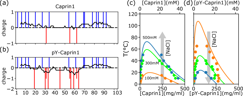
Figure 1: rG-RPA theory predictions rationalize different salt dependence of Caprin1 and pY-Caprin1 LLPS. (a,b) Vertical lines indicate the sequence positions (horizontal variable) of positively charged residues (blue) and negatively charged residues or phosphorylated tyrosines (red) for (a) Caprin1 and (b) pY-Caprin1. (c,d) rG-RPA coexistence curves (phase diagrams, continuous curves color-coded for the NaCl concentrations indicated) agree reasonably well with experiment (dots, same color code). The grey arrows in (c,d) highlight that when [NaCl] increases, LLPS propensity increases for (c) Caprin1 but decreases for (d) pY-Caprin1.

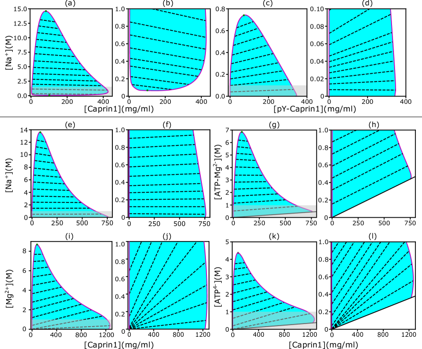
Figure 2: rG-RPA theory predictions rationalize [NaCl]-modulated reentrant phase behavior of Caprin1. In each salt-protein phase diagram, tielines (dashed) connect coexisting phases on the boundary (solid magenta curve) of the cyan-shaded coexistence region. For clarity, zoom-in views of the grey-shaded part in (a, c, e, g, i, k) are provided by the plots to the right, i.e., (b, d, f, h, j, l), respectively. The solid inclined lines in (g, h, k, l) mark the minimum counterion concentrations required for overall electric neutrality of each of the model systems. Results are shown for monovalent cation and anion with Caprin1 (a, b) or pY-Caprin1 (c, d); or monovalent cation and divalent anion with Caprin1 (e–h); or divalent cation and tetravalent anion with Caprin1 (i–l). Cation-modulated reentrant phase behaviors is seen for a wide concentration range for Caprin1 in (a, b) but only a very narrow range of high Caprin1 concentrations in (e, f, i, j).

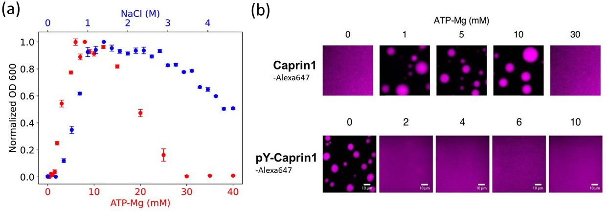
Figure 3: Experimental demonstration of [ATP-Mg]- and [NaCl]-modulated reentrant phase behavior for Caprin1. (a) Turbidity quantified by optical density at 600 nm (OD600) to assess Caprin1 LLPS propensity (vertical scale provides OD600 normalized by peak value) at a Caprin1 concentration of 200 $\mu$M [for ATP-Mg dependence (red), bottom scale] or 300 $\mu$M [for NaCl dependence (blue), top scale], measured at room temperature ($\sim 23^{\circ}$C). Error bars are one standard deviations of triplicate measurements, which in most cases was smaller than the plotting symbols. The ATP-Mg dependence seen here for 200 $\mu$M Caprin1 is similar to the results for 400 $\mu$M Caprin1 (Fig. 6C of ref. LewisPNAS2021 ). (b) Microscopic images of Caprin1 and pY-Caprin1 at varying ATP-Mg concentrations at room temperature, showing reentrant behavior for Caprin1 but not for pY-Caprin1. Each sample contains 200 $\mu$M of either Caprin1 or pY-Caprin1, with 1% of either Caprin1-Cy5 or pY-Caprin1-Cy5 (labeled with Cyanine 5 fluorescent dye) added for visualization, in a 25 mM HEPES buffer at pH 7.4. Scale bars represent 10 $\mu$m. The general trends shown here are consistent with our theoretical and computational predictions.

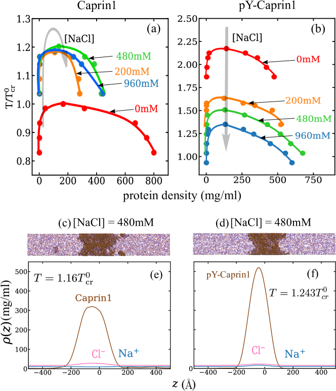
Figure 4: Explicit-ion coarse-grained molecular dynamics simulations rationalize [NaCl]-modulated reentrant behavior for Caprin1 and lack thereof for pY-Caprin1. (a) Simulated phase diagrams (binodal curves) of Caprin1 at different temperatures plotted in units of the critical temperature $T^{0}_{\rm cr}$ for zero [NaCl]. Symbols are simulated data points. Continuous curves are guides for the eye. Grey arrow indicates variation in [NaCl]. (b) Same as (a) but for pY-Caprin1, with the same temperature unit as that in (a). (c) A snapshot showing phase equilibrium between dilute and condensed phases of Caprin1 (brown chains) immersed in Na⁺ (blue) and Cl^- (red) ions simulated at [NaCl] = 480mM. (d) A similar snapshot for pY-Caprin1. (e, f) Density profiles, $\rho(z)$, of Na⁺, Cl^-, and (e) Caprin1 or (f) pY-Caprin1 along the elongated dimension $z$ of the simulation box showing variations of Na⁺ and Cl^- concentrations between the protein-dilute phase (low $\rho$ for protein) and protein-condensed phase (high $\rho$ for protein) at the simulation temperatures indicated.

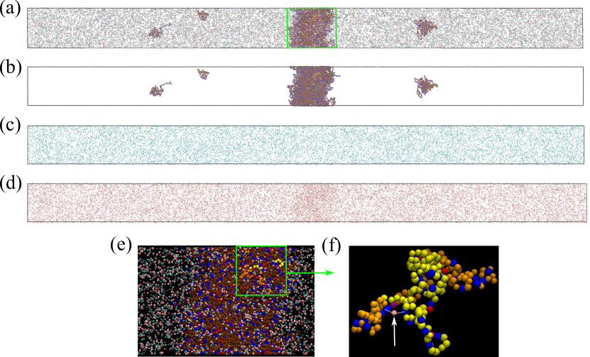
Figure 5: Counterions can stabilize Caprin1 condensed phase by favorable bridging interactions involving a pair of same-charge residues on different chains. (a) Snapshot from explicit-ion coarse-grained molecular dynamics simualtion under LLPS conditions for Caprin1, showing the spatial distributions of Caprin1, Na⁺, and Cl^- (as in Fig. 4c). The three components of the same snapshot are also shown separately in (b), (c), and (d), i.e., (b) Caprin1 alone, (c) Na⁺ alone, and (d) Cl^- alone. (e) A zoom-in view of the condensed droplet [corresponding to the green box in (a)], now with a black background and a different color scheme. (f) A further zoom-in view of the part enclosed by the green box in (e) focusing on two interacting Caprin1 chains. A Cl^- ion (pink bead indicated by the arrow) is seen here interacting favorably with two arginines residues (blue beads) on the two Caprin1 chains (whose uncharged residues are colored differently by yellow or orange, lysine and aspartic acids in both chains are depicted, respectively, as magenta and red beads).

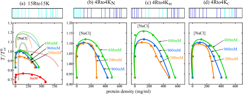
Figure 6: Explicit-ion coarse-grained molecular dynamics simulations rationalize [NaCl]-modulated reentrant behavior for RtoK variants of Caprin1. Four variants studied experimentallyLewisJACS2020 are simulated: (a) 15Rto15K, in which 15 arginines in the wildtype Caprin1 IDR are substituted by lysines, (b) 4Rto4K_N, (c) 4Rto4K_M, and (d) 4Rto4K_C, in which four arginines are substituted by lysines in the (b) N-terminal, (c) middle, and (d) C-terminal regions, respectively. Top panels show positions of the arginines (dark blue) and lysines (cyan) along the Caprin1 IDR sequence. Lower panels are phase diagrams presented in the same style as that in Fig. 4. The phase diagrams for wildtype Caprin1 from Fig. 4a are included as continuous curves with no data points in (a) for comparison. The simulated trend is consistent with experiment.LewisJACS2020

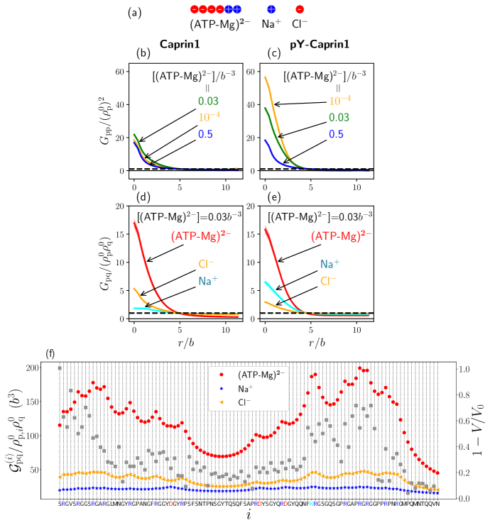
Figure 7: Field-theoretic simulation (FTS) rationalizes experimental observation of Caprin1 sequence position-specific ATP binding. (a) The 6-bead simple model for (ATP-Mg)^2- and the single-bead models for monovalent salt ions used in the present FTS. (b–e) Normalized protein-protein correlation functions at three different [(ATP-Mg)^2-] values (b, c) and protein-ion correlation functions [Eq. (11)] at [(ATP-Mg)${}^{2-}]/b^{-3}$ = 0.03 (d, e) for Caprin1 (b, d) and pY-Caprin1 (c, e), computed for Bjerrum length $l_{\rm B}=7b$. Horizontal dashed lines are unity baselines corresponding to products of overall densities. These FTS-predicted correlation functions rationalize the experimentally observed difference in ATP-Mg dependence of Caprin1 and pY-Caprin1 LLPS (Fig. 3). (f) Values of position-specific integrated correlation ${\cal G}^{(i)}_{\rm pq}/\rho^{0}_{{\rm p},i}\rho^{0}_{\rm q}$ (left vertical axis) correspond to the relative contact frequencies between individual residues ($i$) along the Caprin1 IDR sequence with ${\rm q}=$ (ATP-Mg)^2-, Na⁺, and Cl^- under the same conditions [Eq. (13)] (color symbols). Included for illustration are experimental NMR volume ratios $V/V_{0}$ data on site-specific Caprin1-ATP association.LewisPNAS2021 $V/V_{0}$ decreases with increased contact probability, although a precise quantitative relationship between the two is yet to be determined. Thus, the plotted $1-V/V_{0}$ quantity (grey data-points, right vertical scale), which is expected to correlate with contact frequency, is exhibiting a trend consistent with our FTS prediction.

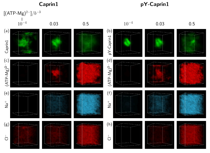
Figure 8: FTS rationalizes colocalization of ATP-Mg within the Caprin1 condensed phase. FTS snapshots are from simulations at $l_{\rm B}=7b$ (same as that for Fig. 7). Spatial distributions of real positive parts of the density fields for the protein (a, b), (ATP-Mg)^2- (c, d), Na⁺ (e, f), and Cl^- (g, h) components of our FTS systems are shown for three different field snapshots each for Caprin1 (left panels) and pY-Caprin1 (right panels) at three different [(ATP-Mg)^2-] values as indicated. Colocalization of (ATP-Mg)^2- with the Caprin1 condensed droplet is clearly seen in the [(ATP-Mg)${}^{2-}]/b^{-3}$ = 0.03 panel of (c).

December 29, 2023

^†Present address: HTuO Biosciences, 610 Main Street, Suite 400, Vancouver, British
^†Present address:  Columbia V6A 2V3, Canada.

^‡Present address: Department of Biochemistry, School of Medicine,
^†Present address:  Case Western Reserve University, Cleveland, Ohio 44106, U.S.A.

^§Contributed equally.

^∗Correspondence information:
^† Hue Sun CHAN.    E-mail: huesun.chan@utoronto.ca
^† Tel: (416)978-2697; Fax: (416)978-8548
^† Department of Biochemistry, University of Toronto, Medical Sciences Building – 5th Fl.,
^† 1 King’s College Circle, Toronto, Ontario M5S 1A8, Canada.

Supplementary Methods

Experimental sample preparation –
Information in addition to that provided in the maintext

Wildtype (WT) Caprin1. As stated in the maintext, WT Caprin1 was used in all reported experiments except those on [NaCl] dependence presented in Table 1 and Fig. 3a. The preparation of sample WT Caprin1 is now briefly described as follows: Caprin1 with an N-terminal His-SUMO tag was produced in BL21 (DE3)-RIPL Codon Plus E. coli cells. These cells were cultured until an optical density at 600 nm (OD600) of 0.6 at 37^∘C and then induced with 0.5 mM IPTG for overnight expression at 23^∘C. The harvested cells were suspended in a lysis buffer containing 6 M guanidine hydrochloride (GuHCl), 25 mM Tris, 500 mM NaCl, 20 mM imidazole, 2 mM $\beta$-mercaptoethanol (BME), at pH 8.0, and lysed via sonication. The supernatant, post-sonication, was applied to Ni-NTA (Cytiva) and washed with lysis, wash (25 mM Tris, 500 mM NaCl, 20 mM imidazole, 2 mM BME, at pH 8.0), and elution (25 mM Tris, 500 mM NaCl, 300 mM imidazole, 2 mM BME, at pH 8.0) buffers. Post-elution, the sample was treated with ULP1 during dialysis against a dialysis buffer (25 mM Tris, 250 mM NaCl, and 2 mM BME at pH 8.0). This step was followed by His-SUMO tag removal through Ni-NTA column chromatography. Final purification of Caprin1 was performed using FPLC with a Superdex 75 16/60 column, equilibrated with a gel filtration buffer (3 M GuHCl, 25 mM Tris, 500 mM NaCl, 2 mM BME, pH 8.0). The protein fractions were then dialyzed twice to remove GuHCl before use in experiments.

Double-mutant (N623T, N630T) variant of Caprin1. Our sample preparation for the double-mutant variant used in [NaCl] dependence studies reported in Table 1 and Fig. 3a proceeded as follows. Purified Caprin1 was first exchanged into buffer (25mM sodium phosphate, pH 7.4) via dialysis and was concentrated to $\sim 6$ mM using 3 kDa centrifugal Amicon concentrators (EMD Millipore). The pH of the concentrated protein was adjusted to 7.4 using concentrated hydrochloric acid. Phase separated samples of Caprin1 were prepared by addition of a concentrated stock solution of NaCl (25mM sodium phosphate, pH 7.4, 4M NaCl) to achieve a bulk salt concentration of 300 mM NaCl. Condensed and dilute phases of Caprin1 were transferred all together into an Eppendorf tube using a syringe. After rigorous vortexing, the phase separated samples were incubated at the desired temperatures using a thermocycler with a heated lid (95^∘C). At least one hour was required to allow droplets to form a large condensed phase droplet at the bottom of the tube.

2 $\mu$L of condensed and dilute phases were pipetted into 48 $\mu$L of a 2.8 M urea solution (U4883, Sigma) in MilliQ water in a 15 mL falcon tube, using a positive and an air displacement pipette, respectively. The outside of the tips were wiped with a KimWipe to remove excess protein, prior to transferring into the urea solutions. Following transfer, the samples were digested for Inductively coupled plasma optical emission spectroscopy (ICP-OES) measurements by the addition of 630 $\mu$L of concentrated nitric acid (67%, NX0407, Sigma) and 630 $\mu$L hydrogen peroxide (95321, Sigma), and incubated in an oven at 60^∘C for 54 hours. Post digestion, the sample tubes were cooled at room temperature and centrifuged. 40 $\mu$L of hydrogen peroxide was then added to the samples. No bubbles were observed, indicating the completion of the digestion process. The samples were then bought up to 12 mL using MilliQ water, to achieve a final nitric acid concentration of 3.5%. Blank samples for the condensed and dilute phases were prepared by pipetting 2 $\mu$L of MilliQ water using a positive and an air displacement pipette, respectively, and subsequently following the digestion protocol described above. Sodium standards (0.1, 0.2, 0.5, 1, 2, 4, 8 and 10 ppm) in 3.5% nitric acid for ICP-OES measurements were prepared by dilution of sodium standard solution (00462, Sigma) with MilliQ water and concentrated nitric acid (67%, NX0407, Sigma). All samples were filtered using 0.22 $\mu$m syringe filters prior to ICP-OES. Condensed and dilute phases were drawn in triplicate at each temperature.

Sequence-specific theory of heteropolymer phase separation –
Summary of key steps in the field-theoretic formulation

The following is a more extensive summary to supplement the brief outline in the Methods section of the maintext provided under the heading “squence-specific theory of heteropolymer phase separation”. Further details are available from our recent publications (e.g., refs. (101; 104) and references therein).

Using the same notation for the partition function ${\cal Z}$ in Eq. (2), the connectivity term $\mathscr{T}$ in Eq. (3), and the total potential energy $\mathscr{U}$ of the maintext, we now provide the precise field-theoretic forms for the Coulomb electrostatic potential $\mathscr{U}_{\rm el}$ and two-body excluded volume interaction $\mathscr{U}_{\rm ex}$ terms in $\mathscr{U}=\mathscr{U}_{\rm el}+\mathscr{U}_{\rm ex}$ by introducing the number density operators

$$\hat{\rho}_{\rm p}({\bf r})= \sum_{\alpha=1}^{n_{\rm p}}\sum_{i=1}^{N}\delta({\bf r}-{\bf R}_{\alpha,i})\;,$$ (S1a)

$$\hat{\rho}_{\rm s}({\bf r})= \sum_{a=1}^{n_{\rm s}}\delta({\bf r}-{\bf r}_{a})\;,$$ (S1b)

$$\hat{\rho}_{\rm c}({\bf r})= \sum_{a={n_{\rm s}}+1}^{{n_{\rm s}}+{n_{\rm c}}}\delta({\bf r}-{\bf r}_{a})\;,$$ (S1c)

for the monomers (residues or beads) of the polymer, salt, and counterion, respectively, where $\delta$ represents the Dirac $\delta$ distribution. Solvent (water) degrees of freedom [$n_{\rm w}$ in Eq. (2) for ${\cal Z}$ in the maintext] are not included in Eq. (S1) above because they are only used for the incompressibility constraint in our rG-RPA formulation as an approximate treatment of excluded volume, and solvents are not treated explicitly at all in the present field-theoretic simulation (FTS), i.e., the $n_{\rm w}$ factor is dropped for FTS. The corresponding charge density operators for the number density operators in Eq. (S1) are

$$\hat{c}_{\rm p}({\bf r})= \sum_{\alpha=1}^{n_{\rm p}}\sum_{i=1}^{N}\sigma_{i}\delta({\bf r}-{\bf R}_{\alpha,i})\;,$$ (S2a)

$$\hat{c}_{\rm s}({\bf r})= z_{\rm s}\sum_{a=1}^{n_{\rm s}}\delta({\bf r}-{\bf r}_{a})=z_{\rm s}\hat{\rho}_{\rm c}\;,$$ (S2b)

$$\hat{c}_{\rm c}({\bf r})= z_{\rm c}\sum_{a={n_{\rm s}}+1}^{{n_{\rm s}}+{n_{\rm c}}}\delta({\bf r}-{\bf r}_{a})=z_{\rm c}\hat{\rho}_{\rm s}\;.$$ (S2c)

For $\hat{c}_{\rm p}$, $\sigma_{i}=+1$ for arginine and lysine, $\sigma_{i}=-1$ for aspartic and glutamic acids, $\sigma_{i}=-2$ for phosphorylated tyrosine, and $\sigma_{i}=0$ for all other amino acid residues in the Caprin1/pY-Caprin1 sequences studied here (as in the maintext). The $\mathscr{U}_{\rm el}$ and $\mathscr{U}_{\rm ex}$ are now given by

$$\mathscr{U}_{\rm el}= \frac{l_{\rm B}}{2}\int d{\bf r}d{\bf r}^{\prime}\Big{[}\hat{c}_{\rm p}({\bf r})+\hat{c}_{\rm s}({\bf r})+\hat{c}_{\rm c}({\bf r})\Big{]}\frac{1}{|{\bf r}-{\bf r}^{\prime}|}\Big{[}\hat{c}_{\rm p}({\bf r}^{\prime})+\hat{c}_{\rm s}({\bf r}^{\prime})+\hat{c}_{\rm c}({\bf r}^{\prime})\Big{]},$$ (S3a)

$$\mathscr{U}_{\rm ex}= \frac{v_{2}}{2}\int d{\bf r}\Big{[}\hat{\rho}_{\rm p}({\bf r})+\hat{\rho}_{\rm s}({\bf r})+\hat{\rho}_{\rm c}({\bf r})\Big{]}^{2},$$ (S3b)

where $l_{\rm B}=e^{2}/(4\pi\epsilon_{0}\epsilon_{\rm r}k_{\rm B}T)$ is Bjerrum length, $v_{2}$ is the interaction parameter for two-body excluded-volume effect, $\epsilon_{0}$ and $\epsilon_{\rm r}$ are vacuum and relative permittivities, respectively, $k_{\rm B}$ is Boltzmann constant, and $T$ is absolute temperature.

As mentioned in the maintext, two conjugates fields, $\psi({\bf r})$ for Coulomb interaction and $\varw({\bf r})$ for excluded volume, are then introduced to linearize the density operators that are quadratic in $\mathscr{U}_{\rm el}$ and $\mathscr{U}_{\rm ex}$ by applying the Hubbard-Stratonovich transformationStrat57 ; Hub59 resulting in a reformulated partition function ${\cal Z}^{\prime}\equiv({n_{\rm p}}!{n_{\rm s}}!{n_{\rm c}}!n_{\rm w}!){\cal Z}$ [with ${\cal Z}$ given by Eq. (2) of maintext] expressed as a functional integral over the fields $\psi$ and $\varw$:

$${\cal Z}^{\prime}=\int\mathscr{D}\psi\mathscr{D}\varw\exp\left[-\int d{\bf r}\left(\frac{\left[\nabla\psi({\bf r})\right]^{2}}{8\pi l_{\rm B}}+\frac{\varw({\bf r})^{2}}{2v_{2}}\right)+{n_{\rm p}}\ln{\cal Q}_{\rm p}+{n_{\rm s}}\ln{\cal Q}_{\rm s}+{n_{\rm c}}\ln{\cal Q}_{\rm c}\right],$$ (S4)

where ${\cal Q}_{\rm p}$, ${\cal Q}_{\rm s}$, and ${\cal Q}_{\rm c}$ are single-molecule partition functions of polymer, salt ion, and counterion, respectively, which are all functionals of $\psi$ and $\varw$:

$${\cal Q}_{\rm p}[\psi,\varw]= \int\prod_{\tau=1}^{N}d{\bf R}_{\tau}\exp\Big{(}-{\cal H}_{\rm p}\left[{\bf R};\psi,\varw\right]\Big{)}$$

$$= \int\prod_{\tau=1}^{N}d{\bf R}_{\tau}\exp\left[-\frac{3}{2l^{2}}\sum_{i=1}^{N-1}\left({\bf R}_{i+1}-{\bf R}_{i}\right)^{2}-{\rm i}\sum_{i=1}^{N}\left(\sigma_{i}\psi({\bf R}_{i})+\varw({\bf R}_{i})\right)\right],$$ (S5a)

$${\cal Q}_{\rm s,c}[\psi,\varw]= \int d{\bf r}\exp\Big{[}-{\rm i}\big{(}z_{s,c}\psi({\bf r})+\varw({\bf r})\big{)}\Big{]}\;,$$ (S5b)

where ${\rm i}$ is the imaginery unit, i.e., ${\rm i}^{2}=-1$.

The ${\cal Z}^{\prime}$ in Eq. (S4) can be analyzed via various field theoretic approaches. Two approaches are utilized in the present work: (i) one-loop perturbation expansion is employed to derive analytical theories based upon random-phase-approximation (RPA), and (ii) field-theoretic simulation (FTS) is conducted to compute observables numerically.

Renormalized-Gaussian random-phase-approximation (rG-RPA) theory

The rG-RPA theory was put forth by some of the present authors.kings2020 For a broad overview, we briefly summarize here the major methodological steps and key results of the theory. Interested readers are referred to ref. (74) for further details.

In our formulation of rG-RPA theory, simplifying assumptions are made to the effect that excluded volume is taken into account only between pairs of different polymer chains (no consideration of intrachain excluded volume) and small ions are treated as point charges. Denoting Boltzmann’s constant as $k_{\rm B}$, absolute temperature as $T$, the input “bare” Kuhn length as $l$, and the total free energy and volume of the system as $F$ and $\Omega$ respectively, the system free energy in units of $k_{\rm B}T$ per volume $l^{3}$ is given by

$$f=\frac{Fl^{3}}{k_{\rm B}T\Omega}=-s+f_{\rm ion}+f_{\rm 0}+f_{\rm p}\;.$$ (S6)

Here $s$ is translational entropy

$$-s=\frac{\phi_{\rm p}}{N}\ln\phi_{\rm p}+\phi_{\rm s}\ln\phi_{\rm s}+\phi_{\rm c}\ln\phi_{\rm c}+\phi_{\rm w}\ln\phi_{\rm w}\;,$$ (S7)

where $\phi_{\rm p}$, $\phi_{\rm s}$, $\phi_{\rm c}$, and $\phi_{\rm w}=1-\phi_{\rm p}-\phi_{\rm s}-\phi_{\rm c}$ are, respectively, volume fractions of polymers, salt ions, counterions, and solvent, with the last equality following from the incompressibility condition that we have stipulated. The $f_{\rm ion}$ term in Eq. (S6) accounts for the free energy of the small ions via the form

$$f_{\rm ion}=-\frac{1}{4\pi}\left[\ln\left(1+\kappa_{\rm D}l\right)-\kappa l+\frac{1}{2}\left(\kappa_{\rm D}l\right)^{2}\right]\;,$$ (S8)

where $1/\kappa_{\rm D}=1/\sqrt{4\pi l_{\rm B}\left(z_{\rm s}^{2}\rho_{\rm s}+z_{\rm c}^{2}\rho_{\rm c}\right)}$ is the Debye screening length. The term $f_{\rm 0}$ in Eq. (S6) is the zeroth-order excluded volume effect given by

$$f_{\rm 0}=\frac{l^{3}}{2}v_{2}\rho_{\rm m}^{2}\;,$$ (S9)

where $\rho_{\rm m}=n_{\rm p}N/\Omega$ is the average monmer (residue or bead) density of the polymers in the system and the expression $f_{\rm p}=-(l^{3}/\Omega)\ln{\cal Z}_{\rm p}$ for the last term in Eq. (S6) is derived from the polymer partition function

$${\cal Z}_{\rm p}=\int\mathscr{D}\psi\mathscr{D}\varw\exp\left[-\int d{\bf r}\left(\frac{\psi({\bf r})\left(-\nabla^{2}+\kappa^{2}\right)^{2}\psi({\bf r})}{8\pi l_{\rm B}}+\frac{\varw({\bf r})^{2}}{2v_{2}}\right)+{n_{\rm p}}\ln{\cal Q}_{\rm p}\right]\;.$$ (S10)

An analytical perturbative field theory may now be derived from ${\cal Z}_{\rm p}$ by considering the Taylor expansion of $\ln{\cal Q}_{\rm p}$ up to the second order of $\psi$ and $\varw$ while omitting terms that do not affect the relative energies of the configurations, viz.,

$$\ln{\cal Q}_{\rm p}\approx-\frac{1}{2}\left[\left\langle\left(\hat{c}_{\rm p}-\overline{c}_{\rm p}\right)^{2}\right\rangle\psi^{2}+\left\langle\left(\hat{\rho}_{\rm p}-\overline{\rho}_{\rm p}\right)^{2}\right\rangle\varw^{2}+2\left\langle\left(\hat{c}_{\rm p}-\overline{c}_{\rm p}\right)\left(\hat{\rho}_{\rm p}-\overline{\rho}_{\rm p}\right)\right\rangle\psi\varw\right]\;,$$ (S11)

where $\overline{c}_{\rm p}$ and $\overline{\rho}_{\rm p}$ are the overall average charge and number densities, respectively, of the polymer [cf. Eqs. (S1) and (S2) above and Eq. (A37) of ref. (74)]. It follows that ${\cal Z}_{\rm p}$ can then be approximated as a Gaussian integral in the Fourier-transformed ${\bf k}$-space,

$${\cal Z}_{\rm p}\approx\int\prod_{{\bf k}\neq{\bf 0}}\sqrt{\frac{\nu_{k}}{v_{2}}}\frac{d\psi_{\bf k}d\varw_{\bf k}}{2\pi\Omega}\exp\left[-\frac{1}{2\Omega}\sum_{{\bf k}\neq{\bf 0}}\langle\psi_{-{\bf k}}\;\varw_{-{\bf k}}|\left(\begin{matrix}\nu_{k}+\rho_{m}{g^{\rm cc}_{{\bf k}}}&\rho_{m}{g^{\rm mc}_{{\bf k}}}\\ \rho_{m}{g^{\rm mc}_{{\bf k}}}&v_{2}^{-1}+\rho_{m}{g^{\rm mm}_{{\bf k}}}\end{matrix}\right)\left|\begin{matrix}\psi_{\bf k}\\ \varw_{\bf k}\end{matrix}\right\rangle\right],$$ (S12)

where ${g^{\rm cc}_{{\bf k}}}$, ${g^{\rm mm}_{{\bf k}}}$, and ${g^{\rm mc}_{{\bf k}}}$ are charge-charge, mass-mass (i.e., matter-matter), and mass-charge (matter-charge) correlation functions in ${\bf k}$-space, and $\nu_{k}=k^{2}/(4\pi l_{\rm B})+(z_{\rm s}^{2}\rho_{s}+z_{\rm c}^{2}\rho_{c})$. The free energy $f_{\rm p}$ is then given by

$$f_{\rm p}=\frac{l^{3}}{2}\int\frac{d^{3}k}{(2\pi)^{3}}\ln\left[1+\rho_{m}\left(\frac{{g^{\rm cc}_{{\bf k}}}}{\nu_{k}}+v_{2}{g^{\rm mm}_{{\bf k}}}\right)+\frac{v_{2}}{\nu_{\bf k}}\rho_{m}^{2}\left({g^{\rm cc}_{{\bf k}}}{g^{\rm mm}_{{\bf k}}}-\left({g^{\rm mc}_{{\bf k}}}\right)^{2}\right)\right].$$ (S13)

The correlation functions in Eq. (S13) may be estimated by various field-theory approximations. In rG-RPA, they are evaluated using a variational approach to the single-polymer partition functon ${\cal Q}_{\rm p}$ by first expressing the Hamiltonian ${\cal H}_{\rm p}$ in Eq. (4) of the maintext as the sum of an approximate Gaussian-chain Hamiltonian with an effective (renormalized) Kuhn length $xl$ (where $l$ is the original “bare” Kuhn length) plus the remaining term, viz.,

$${\cal H}_{\rm p}={\cal H}_{\rm p}^{0}+{\cal H}_{\rm p}^{1}$$ (S14)

where

$${\cal H}_{\rm p}^{0}= \frac{3}{2l^{2}x}\sum_{i=1}^{N-1}\left({\bf R}_{i+1}-{\bf R}_{i}\right)^{2}$$ (S15a)

$${\cal H}_{\rm p}^{1}= \frac{3}{2l^{2}}\left(1-\frac{1}{x}\right)\sum_{i=1}^{N-1}\left({\bf R}_{i+1}-{\bf R}_{i}\right)^{2}-{\rm i}\sum_{i=1}^{N}\left[\sigma_{i}\psi({\bf R}_{i})+\varw({\bf R}_{i})\right]\;$$ (S15b)

are the same equations as Eqs. (5a) and (5b) in the maintext and adopt essentially the same form as the unrenormalized Eq. (S5a). To make progress, we take the polymer square end-to-end distance ${\bf R}_{\rm EE}^{2}$ as a key physical observable and require its thermodynamic average to be produced by ${\cal H}_{\rm p}^{0}$ in good approximation. Based on this premise, a variational theory as described in ref. (48) is applied to calculate the $x$ parameter in the above Eq. (S15). Details of the derivation are given in the Appendices of ref. (74). Here we show only the variational equation for solving $x$:

$$1-\frac{1}{x}-\frac{Nl^{3}}{18(N-1)}\int\frac{d^{3}k}{(2\pi)^{3}}\frac{k^{2}\Xi_{k}^{x}}{\det\Delta_{k}^{x}}=0\;,$$ (S16)

where $\Delta_{k}^{x}$ is the $2\times 2$ matrix in Eq. (S12) with $l\rightarrow xl$ (renormalized Kuhn length), $|i-j|\rightarrow|i-j|/x$ (renormalized contour length) and thus $l^{2}|i-j|\rightarrow l^{2}x|i-j|$ such that the correlation functions in $\Delta_{k}^{x}$ becomekings2020

$${g^{\rm cc}_{{\bf k}}}\to {g^{\rm cc}_{k,x}}=\frac{1}{N}\sum_{i,j=1}^{N}\sigma_{i}\sigma_{j}e^{-\frac{1}{6}(kl)^{2}x|i-j|}$$ (S17a)

$${g^{\rm mm}_{{\bf k}}}\to {g^{\rm mm}_{k,x}}=\frac{1}{N}\sum_{i,j=1}^{N}e^{-\frac{1}{6}(kl)^{2}x|i-j|}$$ (S17b)

$${g^{\rm mc}_{{\bf k}}}\to {g^{\rm mc}_{k,x}}=\frac{1}{N}\sum_{i,j=1}^{N}\sigma_{i}e^{-\frac{1}{6}(kl)^{2}x|i-j|},$$ (S17c)

and the $\Xi_{k}^{x}$ in the integrand on the right hand side of Eq. (S16) is now given by

$$\Xi_{k}^{x}=\frac{\bar{\xi}_{k}^{x}}{v_{2}}+\nu_{k}\bar{g}_{k}^{x}+\rho_{m}\left(\bar{\xi}_{k}^{x}{g^{\rm mm}_{k,x}}+\bar{g}_{k}^{x}{g^{\rm cc}_{k,x}}-2\bar{\zeta}_{k}^{x}{g^{\rm mc}_{k,x}}\right)$$ (S18)

where

$$\bar{\xi}_{k}^{x}= \frac{1}{N}\sum_{i,j=1}^{N}|i-j|^{2}\sigma_{i}\sigma_{j}e^{-\frac{1}{6}(kl)^{2}x|i-j|}\;,$$ (S19a)

$$\bar{g}_{k}^{x}= \frac{1}{N}\sum_{i,j=1}^{N}|i-j|^{2}e^{-\frac{1}{6}(kl)^{2}x|i-j|}\;,$$ (S19b)

$$\bar{\zeta}_{k}^{x}= \frac{1}{N}\sum_{i,j=1}^{N}|i-j|^{2}\sigma_{i}e^{-\frac{1}{6}(kl)^{2}x|i-j|}\;.$$ (S19c)

Because the above field theory is formulated to focus only on sequence-specific electrostatics and excluded volume, in the form presented above it does not account for short-range attractions such as those arising from $\pi$-related and hydrophobic effects; but we need to take these effects into consideration to arrive at a more direct comparison between rG-RPA predictions and experiments, e.g., as those provided in Fig. 1c,d of the maintext. To account for these interactions approximately in Caprin1, particularly the interactions involving $\pi$-electrons,LewisPNAS2021 , we introduce, as before,linPRL a temperature-dependent Flory-Huggins interaction to augmented the free energy $f$ in Eq. (S6),kings2020 ; SumanPNAS resulting in an overall total free energy

$$f=-s+f_{\rm ion}+f_{\rm 0}+f_{\rm p}-\left(\Delta h\frac{l_{\rm B}}{l}-\Delta s\right)\rho_{\rm m}^{2}\;,$$ (S20)

where $\Delta h$ and $\Delta s$ are the enthalpic and entropic components, respectively, of the mean-field Flory-Huggins interaction for favorable non-electrostatic attraction. With this augmented rG-RPA+FH system free energy $f$ in hand, we solve the solute and solvent concentrations in dilute and condensed phases by balancing the chemical potentials of each solute components and the osmotic pressures in the two phases. When the salt concentration is assumed for simplicity to be uniform throughout the system (Fig. 1c,d of the maintext), the system only has $\rho_{\rm m}$ as a variable and the binodal phase separation concentrations are readily obtained by solving the standard common tangent conditions.MiMB2023 ; linJML The Flory-Huggins parameters $\Delta h$ and $\Delta s$ fitted to the experimental data are $\Delta h=1.08$ kcal mol^-1, $\Delta s=0$ for the Caprin1 phase diagrams in Fig. 1c and $\Delta h=1.08$ kcal mol^-1, $\Delta s=-29.8$ kcal mol^-1K^-1 for the pY-Caprin1 phase diagrams in Fig. 1d. When the uniform salt concentration restriction is removed to allow for fully varying salt and polymer concentrations (Fig. 2 of the maintext), the final concentrations in the two phases depend on their initial bulk (overall) concentrations. The corresponding two-dimensional, polymer-salt phase diagram (at a given temperature $T$) is obtained by similar balancing conditions.njp2017 As stated in the maintext, the two-dimensional rG-RPA phase diagrams in Fig. 2 are for $T=300$ K.

Explicit-ion coarse-grained explicit-chain molecular dynamics (MD) simulation

Coarse-grained MD simulations are performed with the GPU version of HOOMD-Blue software hoomd_blue_1 ; anderson_etal2008 using the slab method that has been developed recently to allow for simulations of relatively large number of polymerspanag2017 and applied to liquid-liquid phase separation (LLPS) of intrinsically disordered proteins (IDPs).dignon18 This general MD protocol has been utilized extensively,mittal19 ; Mpipi including by our group.SumanPNAS ; suman2

Within the methodological framework of this coarse-grained simulation protocol, we introduce explicit small ions into our present simulations because they are necessary to account for subtle experimental observations that are not readily reproduced by using implicit-ion electrostatic screening. Simulations in the present study are performed with 100 chains of the Caprin1 IDR (wildtype or variants) at four salt ([NaCl]) concentrations: (i) at [NaCl] = 0 where the system is neutralized by adding appropriate number (1,300) of chloride ($\mathrm{Cl^{-}}$) ions, (ii) neutralized and at [NaCl] = 200 mM by adding 15,000 pairs of explicit Na⁺ and Cl^- ions, (iii) neutralized and at [NaCl] = 480 mM by adding the same number of 15,000 pairs of explicit Na⁺ and Cl^- ions, and (iv) neutralized and at [NaCl] = 960 mM again with 15,000 pairs of explicit Na⁺ and Cl^- ions. As will be described below, specific small-ion concentrations in (ii), (iii), and (iv) are implemented by varying the size of the final simulation box. A similar procedure is used for simulation of pY-Caprin1 IDR phase behaviors under these four [NaCl] values. Because each pY-Caprin1 IDR has a net $-1$ charge, the only difference with the Caprin1 IDR simulation is that neutralization of the pY-Caprin1 chain requires 100 Na⁺ ions instead of 1,300 Cl^- ions. The amino acid sequences simulated using coarse-grained MD in the present study are provided in Supplementary Fig. S1.

Coarse-grained MD interaction potentials. As before,SumanPNAS ; dignon18 each amino acid residue is modeled as a single bead. Beads representing different amino acid residues have different masses, sizes, and engage in pairwise interactions with different strengths.SumanPNAS ; dignon18 Following the notations of our earlier simulation worksSumanPNAS ; suman2 ; suman1 , we consider $n_{\rm p}$ number of polymers labeled as $\mu$, $\nu$ = 1, 2, …$n_{\rm p}$, with each polymer consisting of $N$ number of beads labeld by $i,j=1,2,\dots,N$, and $n_{\rm c}$ number of counterions to neutralize the charged polymers.

For salt-dependent LLPS, we consider $n_{+}$ small (salt) cations and $n_{-}$ small (salt) anions. These small ions are labeled, respectively, by $\gamma=1,2,\dots,n_{+}$ and $\beta=1,2,\dots,n_{-}$, and they correspond to Na⁺ and Cl^- in the present coarse-grained MD simulations. As stated in the maintext, our total MD potential energy is the sum of electrostatic (el), short-spatial-range (sr) Lennard-Jones (LJ)-type, and bonding (bond) interactions:

$$U_{\rm T}=U_{\rm el}+U_{\rm sr}+U_{\rm bond}\;.$$ (S21)

For our systems of interest, the electrostatic part is a sum of polymer-polymer (pp), polymer-small ion (pi), and small ion-small ion (ii) contributions:

$$U_{\rm el}=U_{\rm el,pp}+U_{\rm el,pi}+U_{\rm el,ii}$$ (S22)

As stated in the maintext [Eq. (6)], the polymer-polymer potential energy is

$$U_{\rm el,pp}=\frac{e^{2}}{8\pi\epsilon_{0}\epsilon_{\rm r}}{\sum_{\mu,\nu=1}^{n_{p}}\sum_{i,j=1}^{N}}\Bigl{(}1-\delta_{\mu\nu}\delta_{ij}\Bigr{)}\frac{\sigma_{i}\sigma_{j}}{r_{{\mu}i,{\nu}j}}\;,$$ (S23)

where $e$ is protonic charge, $\epsilon_{0}$ is vacuum permittivity, $\epsilon_{\rm r}$ is relative permittivity (dielectric constant), and $r_{{\mu}i,{\nu}j}$ is the spatial distance between the $i$th residue of the $\mu$th polymer and the $j$th residue of the $\nu$th polymer. The Kronecker symbol $\delta$ signals exclusion of the self-interacting $\mu=\nu$, $i=j$ terms in the summations (irrespective of the values of these terms) because $1-\delta_{xy}=0$ if $x=y$ and $1-\delta_{xy}=1$ otherwise. In units of the protonic charge $e$, $\sigma_{i}$ of unphosphorylated amino acid residue beads are taken from ref. (91). Except lysine and arginine ($\sigma_{i}=+1$), glutamic and aspartic acid ($\sigma_{i}=-1$), histidine ($\sigma_{i}=+0.5$), note that there is no histidine in the Caprin1/pY-Caprin1 sequences simulated here) and phosphorylated tyrosine ($\sigma_{i}=-2$), all other amino acid residues are assigned zero charge.

As stated in the maintext, the electrostatic interactions between polymers and small ions is given by

$$U_{\rm el,pi}=\frac{e^{2}}{4\pi\epsilon_{0}\epsilon_{\rm r}}\sum_{\mu=1}^{n_{\rm p}}\sum_{i=1}^{N}\left\{\sum_{k=+,-}\left[\sum_{\gamma(k)=1}^{n_{\gamma}(k)}\frac{\sigma_{i}\sigma_{k}}{r_{{\mu}i,\gamma(k)}}\right]\right\}=\frac{e^{2}}{4\pi\epsilon_{0}\epsilon_{\rm r}}\sum_{\mu=1}^{n_{\rm p}}\sum_{i=1}^{N}\left[\sum_{\gamma=1}^{n_{+}}\frac{\sigma_{i}\sigma_{+}}{r_{{\mu}i,\gamma}}+\sum_{\beta=1}^{n_{-}}\frac{\sigma_{i}\sigma_{-}}{r_{{\mu}i,\beta}}\right]\;,$$ (S24)

where the two terms in the $\sum_{k}$ summation in maintext Eq. (7) (enclosed in curly brackets here) are now written explicity, $r_{{\mu}i,\gamma/\beta}$ is the spatial distance between the $i$th residue of the $\mu$th polymer chain and the $\gamma/\beta$ ($\gamma$ or $\beta$)-labeled positive/negative small ion, with $\sigma_{+}$ and $\sigma_{-}$ being the charges of the small positive and negative small ions, respectively. Following ref. (170), we take $\sigma_{+}=+1$ for Na⁺ and $\sigma_{-}=-1$ for Cl^-. Depending on the net charge of the polymer, counterions can be included in either the $n_{+}$ or $n_{-}$ count. For instance, for the positive charged Caprin1 IDR, the total number $n_{-}$ of negatively charged small ions (Cl^-) includes the numbers $n_{\rm c}$ counted as counterions and $n_{\rm s}$ counted as salt ions. As stated in the maintext [Eq. (8)], the electrostatic interaction between the small ions is given by

$$U_{\rm el,ii}=\frac{e^{2}}{8\pi\epsilon_{0}\epsilon_{\rm r}}\sum_{k,k^{\prime}=+,-}\left[\sum_{\alpha(k)=1}^{n_{\alpha}(k)}\sum_{\alpha^{\prime}(k^{\prime})=1}^{n_{\alpha}^{\prime}(k^{\prime})}\Bigl{(}1-\delta_{kk^{\prime}}\delta_{\alpha(k)\alpha^{\prime}(k^{\prime})}\Bigr{)}\frac{\sigma_{k}\sigma_{k^{\prime}}}{r_{\alpha(k),\alpha^{\prime}(k^{\prime})}}\right]\;,$$ (S25)

which is equivalent to

$$U_{\rm el,ii}=\frac{e^{2}}{4\pi\epsilon_{0}\epsilon_{\rm r}}\left[\sum_{\gamma=1}^{n_{+}-1}\sum_{\gamma^{\prime}=\gamma+1}^{n_{+}}\frac{\sigma_{+}^{2}}{r_{\gamma\gamma^{\prime}}}+\sum_{\beta=1}^{n_{-}-1}\sum_{\beta^{\prime}=\beta+1}^{n_{-}}\frac{\sigma_{-}^{2}}{r_{\beta\beta^{\prime}}}+\sum_{\gamma=1}^{n_{+}}\sum_{\beta=1}^{n_{-}}\frac{\sigma_{+}\sigma_{-}}{r_{\gamma\beta}}\right]\;,$$ (S26)

where $r_{xy}$ is the spatial distance between a pair of small ions labeled by $x$ and $y$. As rationalized previouslySumanPNAS in the context of experimental measurements of dielectric properties of biological systems,tros_etal2017 we use $\epsilon_{\rm r}=40$, a value lower than the $\sim 80$ dielectric constant of bulk water, for all simulations reported in the present work.

Short-spatial-range non-bonded LJ interactions are similarly constituted by three components, viz., those for polymer-polymer ($U_{\rm sr,pp}$), polymer-small ion ($U_{\rm sr,pi}$), and small ion-small ion ($U_{\rm sr,ii}$) interactions:

$$U_{\rm sr}=U_{\rm sr,pp}+U_{\rm sr,pi}+U_{\rm sr,ii}\;.$$ (S27)

Here we adopt the Kim-Hummer (KH)KH interaction scheme for $U_{\rm sr,pp}$. KH is based on the Miyazawa-Jernigan (MJ) statistical potentialMJ96 derived from folded globular protein structures in the Protein Data Bank (PDB) and is therefore expected to reflect the energetics of polypeptides, especially the driving forces pertinent to protein folding, its limitationsSumanPNAS notwithstanding. Our previous work shows that the KH potential is adequate for rationalizing the rank ordering of LLPS propensities of the N-terminal IDR of DEAD-box RNA helicase Ddx4 and its charge scrambled and arginine-to-lysine (RtoK) variants. KH also rationalizes the rank ordering of LLPS propensities of WT and an RtoK variant of LAF-1.SumanPNAS We therefore stipulate that the KH interaction scheme is appropriate, at least as a first approximation, to address the LLPS propensities of Caprin1 and its RtoK variants. As before, $U_{\rm sr,pp}$ takes the following formSumanPNAS ; dignon18 :

$$\begin{split}U_{\rm sr,pp}&=\frac{1}{2}{\sum_{\mu,\nu=1}^{n_{p}}\sum_{i,j=1}^{N}}\Bigl{(}1-\delta_{\mu\nu}\delta_{ij}\Bigr{)}(U_{\rm KH})_{{\mu}i,{\nu}j}\;,\\ (U_{\rm KH})_{{\mu}i,{\nu}j}&=U_{\rm LJ}+(1-\lambda_{ij}^{\rm KH})\,\epsilon_{ij}\,\quad\mathrm{if}\,r\leq 2^{1/6}\,a_{ij}\\ &=\lambda_{ij}^{\rm KH}U_{\rm LJ}\,\quad\quad\quad\quad\quad\quad\mathrm{otherwise}\end{split}$$ (S28)

in which

$$(U_{\rm LJ})_{{\mu}i,{\nu}j}=U_{\rm LJ}(\epsilon_{{\mu}i,{\nu}j},a_{{\mu}i,{\nu}j},r_{{\mu}i,{\nu}j})=4\epsilon_{{\mu}i,{\nu}j}\left[\left(\frac{a_{{\mu}i,{\nu}j}}{r_{{\mu}i,{\nu}j}}\right)^{12}-\left(\frac{a_{{\mu}i,{\nu}j}}{r_{{\mu}i,{\nu}j}}\right)^{6}\right]$$ (S29)

and $a_{{\mu}i,{\nu}j}=a_{ij}=(a_{i}+a_{j})/2$, where the van der Waals diameters $a_{i}$ and $a_{j}$, depend only, respectively, on the amino acid residue type (one of twenty) for residue $i$ and residue $j$ (Table S1 of ref. (91)). In contrast, the parameters $\lambda_{ij}^{\rm KH}$ and $\epsilon_{{\mu}i,{\nu}j}=\epsilon_{ij}$ depend on both the residue types of residues $i$ and $j$. Values for $\epsilon_{ij}$ are provided in Table S3 of ref. (91). The formula for $\lambda_{ij}^{\rm KH}=\pm 1$ is given by Eq. (5) of ref. (91) as well as Eqs. (S10) and (S11) of ref. (98).

For the LJ interactions between polymers and small ions, we recognize that while the coarse-grained KH parameters are based on statistical analysis of known folded protein structures, LJ interaction parameters for small ions are typically scaled to match certain physical and chemical properties.cheatham2008 Thus it is not straightforward to postulate an interaction scheme based upon first principles. To make progress and to maintain simplicity of our model, we adopt the LJ form [$U_{\rm LJ}$ in Eq. (S29)] for $U_{\rm sr,pi}$ with a uniform $\epsilon_{{\mu}i,{\nu}j}=\epsilon_{ij}=0.142$ (denoted $\epsilon_{{\rm p}\pm}\equiv 0.142$) for all residue-small ion pairs. This $\epsilon_{ij}=\epsilon_{{\rm p}\pm}$ value is equal to that for a pair of alanine residues in the KH potential and is neither too strong nor too weak among $\epsilon_{ij}$ values for pairwise interactions between amino acid residues. Accordingly,

$$U_{\rm sr,pi}=\sum_{\mu=1}^{n_{\rm p}}\sum_{i=1}^{N}\left[\sum_{\gamma=1}^{n_{+}}U_{\rm LJ}(\epsilon_{{\rm p}\pm},a_{i+},r_{{\mu}i,\gamma})+\sum_{\beta=1}^{n_{-}}U_{\rm LJ}(\epsilon_{{\rm p}\pm},a_{i-},r_{{\mu}i,\beta})\right]\;,$$ (S30)

where $a_{i+}=(a_{i}+a_{+})/2$, $a_{i-}=(a_{i}+a_{-})/2$, with $a_{+}$ and $a_{-}$ being, respectively, the van der Waals diameters of the positively and negatively charged small ions. For the present MD simulations, $a_{+}=a_{{\rm Na}^{+}}$, $a_{-}=a_{{\rm Cl}^{-}}$, and their values are adopted from ref. (170). Similarly, for small ion-small ion LJ interactions,

$$U_{\rm el,ii}=\Biggl{[}\sum_{\gamma=1}^{n_{+}-1}\sum_{\gamma^{\prime}=\gamma+1}^{n_{+}}U_{\rm LJ}(\epsilon_{+},a_{+},r_{\gamma,\gamma^{\prime}})+\sum_{\beta=1}^{n_{-}-1}\sum_{\beta^{\prime}=\beta+1}^{n_{-}} U_{\rm LJ}(\epsilon_{-},a_{-},r_{\beta,\beta^{\prime}})$$ (S31)

$$+ \sum_{\gamma=1}^{n_{+}}\sum_{\beta=1}^{n_{-}}U_{\rm LJ}(\epsilon_{+-},a_{+-},r_{\gamma,\beta})\Biggr{]}\;,$$

where $\epsilon_{+}$ and $\epsilon_{-}$ are, respectively, the LJ interaction energy parameter for the positively and negatively charged small ions, $\epsilon_{+-}=(\epsilon_{+}\epsilon_{-})^{1/2}$, and $a_{+-}=(a_{+}+a_{-})/2$. For the present MD simulations, the $\epsilon_{+}=\epsilon_{{\rm Na}^{+}}$ and $\epsilon_{-}=\epsilon_{{\rm Cl}^{-}}$ values are adopted from ref. (170).

As before, the bond-length energy term $U_{\rm bond}$ in Eq. (S21) for chain connectivity is modeled by a harmonic potential,

$$U_{\rm bond}=\frac{K_{\rm bond}}{2}\sum_{\mu=1}^{{n_{\rm p}}}\sum_{i=1}^{N-1}(r_{{\mu}i,{\nu}i+1}-l)^{2}\;.$$ (S32)

Following previous studies,SumanPNAS ; dignon18 , Kuhn length $l=\mathrm{3.8\,\AA}$ is taken as the C_α–C_α virtual bond length for trans polypeptides and $K_{\rm bond}=10$ kJmol^-1Å^-2.

Simulation protocol. In each of our coarse-grained MD simulations, the IDR chains and ions are initially placed randomly in a sufficiently large cubic box of dimensions $300\times 300\times 300$ ų. Energy minimization is then performed using the FIRE algorithm (available in the HOOMD-Blue package) which includes removal of steric clashes among the initially placed amino acid beads. Next, the system is compressed at a low temperature of 100 K at 1 atm pressure for a period of 50 ns using the Martyna-Tobias-Klein (MTK) thermostat and barostatklein1994 ; tuckerman_etal2006 with a coupling constant of 1 ps. The equations of motion are integrated using velocity-Verlet algorithm with a timestep of 20 fs. Periodic boundary conditions are applied in all three directions. The electrostatic interaction is computed using the PPPM algorithmlebard2012 available in the package. We use a cut-off distance of 15 $\mathrm{\AA}$ for the short-spatial-range non-bonded interactions. After this initial $NPT$ step, we compress the simulation box again along the three dimensions for a period of 50 ns until it reaches a sufficiently high density, using Langevin dynamics for an $NVT$ ensemble with a friction coefficient of $\mathrm{1\,ps^{-1}}$. At the end of this compression step, the dimensions of the simulation box for Caprin1 and its four RtoK variants are $115\times 115\times 115$ ų for [NaCl] = 0 (no small ions beside counterions) and $155\times 155\times 155$ ų for [NaCl] = 200 mM, 480 mM, and 960 mM. For pY-Caprin1, the corresponding dimensions are $115\times 115\times 115$ ų for [NaCl] = 0 (no small ions beside counterions) and $150\times 150\times 150$ ų for [NaCl] = 200 mM, 480 mM, and 960 mM. Next, the system is expanded along one of the spatial dimensions (taken as the $z$-axis) using isotropic linear scaling for 10 ns while keeping the temperature constant at 100 K. For Caprin1 and its four RtoK variants, the simulation box length in the $z$-direction is expanded 14 times for [NaCl] = 0, $33.6$ times for [NaCl] = 200 mM, 14 times for [NaCl] = 480 mM, and 7 times for [NaCl] = 960 mM. For pY-Caprin1, the expansion factors along the $z$-direction are 10 times for [NaCl] = 0, $37.07$ times for [NaCl] = 200 mM, $15.47$ times for [NaCl] = 480 mM, and $7.73$ times for [NaCl] = 960 mM. Note that the simulation box volumes for Caprin1, its RtoK variants, and pY-Caprin1 after this last expansion are identical for the same [NaCl] because the same numbers of polymer chains and small ions are used. The practical reason for keeping the number of Na⁺ and Cl^- ions constant for the higher salt concentration in to minimize computational cost. In other words, the three salt concentrations (200 mM, 480 mM and 960 mM) are achieved here by using different box dimensions. After the last box expansion, $NVT$ equilibration using the Langevin thermostat with a friction coefficient of 1 ps^-1 is performed for 2 $\mathrm{\mu}$s at various temperatures. Final production run is then carried out for another 4 $\mathrm{\mu}$s with the same Langevin thermostat using a much lower friction coefficient of 0.01 ps^-1 for sampling efficiency. The snapshots are saved every 1 ns for further analysis. Detailed descriptions of how to construct a phase diagram from simulation trajectories are provided in ref. (91) and our previous works.MiMB2023 ; SumanPNAS This simulation protocol and the above-described coarse-grained MD model are used to produce the phase diagrams, distributions, and snapshots in Figs. 4–6 of the maintext and Supplementary Fig. S3.

Field-theoretic simulation (FTS) for multiple-component LLPS

Biomolecular condensates in vivo can contain hundreds of protein and nucleic acid species. Therefore, to address their biophysical properties and biochemical functions, theories—starting with rudimentary constructions—are needed for multiple-component LLPS. As a first appproximation and an initial conceptual tool, we find it valuable to utilize FTS—especially recently developed FTS approaches for biomolecular LLPSFredrickson2002 ; Fredrickson2006 ; joanJPCL2019 ; Pal2021 and their extensions—to gain insights into the energetic basis of sequence-specific spatial distributions of various biomolecular components in and out of phase-separated condensates.

FTS enjoys the fundamental advantage that it is not limited by some of the approximations in analytical theories such as RPA and rG-RPA because FTS accounts fully for all field fluctuations in principle. FTS is thus a valuable alternative to analytical theories, though it is computationally more costly in practice and can be impeded by lattice-related artifacts and limitations arising from the small FTS simulation box sizes necessitated by numerical tractability. We view analytical theories and FTS as complementary.

The starting point of FTS is a statistical field theory [e.g., Eq. (S4), which is equivalent to maintext Eq. (9)]. As explained in the maintext, to avoid numerical instabilities, we treat polymer beads and ions as (smeared) Gaussian distributionsWang2010 instead of the point particles stipulated by the Dirac $\delta$-functions in Eqs. (S1) and (S2). For simplicity, this regularization is implemented using a common component-independent width $\bar{a}$ irrespective of chemical species by making the general replacements $\delta({\bf r}-{\bf r}_{a})\rightarrow\Gamma({\bf r}-{\bf r}_{a})$ and $\delta({\bf r}-{\bf R}_{\alpha,i})\rightarrow\Gamma({\bf r}-{\bf R}_{\alpha,i})$, in Eqs. (S1) and (S2) where $\Gamma({\bf r})=e^{-r^{2}/2\bar{a}^{2}}/(2\pi\bar{a}^{2})^{3/2}$, $r^{2}=|{\bf r}|^{2}$.

A general field-theoretic Hamiltonian applicable to a system comprising of one or more charged polymer species including Caprin1, pY-Caprin1, (ATP-Mg)^2- (maintext Fig. 7a), ATP^4- and small ions such as Na⁺, Cl^-, and Mg²⁺ is given by

$$H[\varw,\psi]=\int d{\bf r}\left(\frac{\left(\nabla\psi({\bf r})\right)^{2}}{8\pi l_{\rm B}}+\frac{\varw({\bf r})^{2}}{2v_{2}}\right)-\sum_{m}n_{m}\ln{\cal Q}_{m}[\breve{\varw},\breve{\psi}]\;,$$ (S33)

where the ${\cal Q}_{m}$ functionals ($m$ labels system components) are in general complex when evaluated beyond quadratic order in the fields. Equation (S33) above is identical to Eq. (9) of maintext and formally equivalent to the Hamiltonian in Eq. (S4). Because of the above-described Gaussian smearing, the fields in the arguments of ${\cal Q}_{m}$ are now convoluted with $\Gamma$, i.e. $\phi({\bf r})\rightarrow\breve{\phi}({\bf r})=\Gamma\star\phi({\bf r})\equiv\int d{\bf r}^{\prime}\Gamma({\bf r}-{\bf r}^{\prime})\phi({\bf r}^{\prime})$, where the generic $\phi=\varw,\psi$.

Complex Langevin evolution in fictitious time. A simulation approach developed in the 1980s to handle the complex nature of $H[\varw,\psi]$ and obtain statistical (Boltzmann) averages is the Complex Langevin (CL) method,Parisi1983 ; Klauder1983 which analytically continues the fields $\varw$ and $\psi$ into their respective complex planes and introduces an fictitious (artificial, unphysical) time-coordinate $t$ on which $\varw({\bf r},t)$ and $\psi({\bf r},t)$ now depend. The CL time evolution is governed by stochastic Langevin differential equations [maintext Eq. (10)], as follows:

$$\frac{\partial\phi({\bf r},t)}{\partial t}=-\frac{\delta H}{\delta\phi({\bf r},t)}+\eta_{\phi}({\bf r},t)\;,\quad\phi=\varw,\psi\;,$$ (S34)

where $\eta_{\phi}({\bf r},t)$ is real-valued Gaussian noise with zero mean:

$$\langle\eta_{\phi}({\bf r},t)\eta_{\phi^{\prime}}({\bf r}^{\prime},t^{\prime})\rangle=2\delta_{\phi,\phi^{\prime}}\delta({\bf r}-{\bf r}^{\prime})\delta(t-t^{\prime})\;.$$ (S35)

Thermal averages of any thermodynamic observable $\hat{\cal O}[{\bf R},{\bf r}]$ can then be computed in the field picture (indicated by “$\langle\dots\rangle_{\rm F}$” with subscript “F”) using a corresponding field operator $\tilde{\cal O}[\varw,\psi]$ through averages over all possible equilibrium field configurations, which in turn translate into asymptotic CL time averages with no final dependence on the fictitious time variable $t$, i.e.,

$$\langle\tilde{\cal O}[\varw,\psi]\rangle_{\rm F}\equiv\frac{\int\mathscr{D}\varw\int\mathscr{D}\psi\,\tilde{\cal O}[\varw,\psi]\,e^{-H[\varw,\psi]}}{\int\mathscr{D}\varw\int\mathscr{D}\psi\,e^{-H[\varw,\psi]}}=\lim_{t_{\rm max}\rightarrow\infty}\frac{1}{t_{\rm max}}\int_{0}^{t_{\rm max}}dt\,\tilde{\cal O}[\varw({\bf r},t),\psi({\bf r},t)]\;.$$ (S36)

The Langevin Eq. (S34) involves functional derivatives of the Hamiltonian with respect to the complex fields, which are formally evaluated as

$$\frac{\delta H}{\delta\varw({\bf r})}=\, {\rm i}\sum_{m}\tilde{\rho}_{m}({\bf r})+\frac{1}{v_{2}}\varw({\bf r})\;,$$ (S37a)

$$\frac{\delta H}{\delta\psi({\bf r})}=\, {\rm i}\sum_{m}\tilde{c}_{m}({\bf r})-\frac{1}{4\pi l_{\rm B}}\nabla^{2}\psi({\bf r})\;,$$ (S37b)

where

$$\tilde{\rho}_{m}({\bf r})=\, {\rm i}n_{m}\frac{\delta\ln{\cal Q}_{m}[\breve{\varw},\breve{\psi}]}{\delta\varw({\bf r})}\;,$$ (S38a)

$$\tilde{c}_{m}({\bf r})=\, {\rm i}n_{m}\frac{\delta\ln{\cal Q}_{m}[\breve{\varw},\breve{\psi}]}{\delta\psi({\bf r})}$$ (S38b)

are field operators corresponding, respectively, to number- and charge density of chemical component $m$.

Number density correlation functions. Information about the polymer-polymer, polymer-ion, ion-ion association and ion partitioning into the condensate can be gleaned from number density-number density correlation functions [maintext Eq. (11)]

$$G_{m,n}(|{\bf r}-{\bf r}^{\prime}|)=\langle\hat{\rho}_{m}({\bf r})\hat{\rho}_{n}({\bf r}^{\prime})\rangle\,,$$ (S39)

which can be computed in field theory Pal2021 as

$$G_{m,n\neq m}(|{\bf r}-{\bf r}^{\prime}|)=\, \langle\tilde{\rho}_{m}({\bf r})\tilde{\rho}_{n}({\bf r}^{\prime})\rangle_{\rm F}\;,$$ (S40a)

$$G_{m,m}(|{\bf r}-{\bf r}^{\prime}|)=\, \frac{{\rm i}}{v_{2}}\langle\tilde{\rho}_{m}({\bf r})\varw({\bf r}^{\prime})\rangle_{\rm F}-\sum_{n\neq m}\langle\tilde{\rho}_{m}({\bf r})\tilde{\rho}_{n}({\bf r}^{\prime})\rangle_{\rm F}\;.$$ (S40b)

In some situations, the physical implications of density-density correlation functions $G_{m,n}(r)$ are more apparent when normalized by the component bulk densities $\rho_{m}^{0}$ and $\rho^{0}_{n}$, as discussed in the maintext in connection with the correlation functions shown in Fig. 7.

For small ions that are each represented by a single Gaussian distribution, the density operator is given by

$$\tilde{\rho}_{m}({\bf r})=\frac{n_{m}}{\Omega{\cal Q}_{k}}\Gamma\star e^{-{\rm i}[\breve{\varw}({\bf r})+z_{m}\breve{\psi}({\bf r})]},$$ (S41)

and the charge density operator is $\tilde{c}_{m}({\bf r})=z_{m}\tilde{\rho}_{m}({\bf r})$, where $z_{m}$ is the charge of ion species $m$ and, as defined above, $\Omega$ is the system volume. For polymers (denoted “p”), the density and charge-density operators are calculated using forward (subscript “$F$”) and backward (subscript “$B$”) chain propagators $q_{F}({\bf r},i)$ and $q_{B}({\bf r},i)$ as follows, with $i$ being the label for the beads/monomers along the polymer chain:

$${\cal Q}_{\rm p}=\, \frac{1}{\Omega}\int d{\bf r}\;q_{F}({\bf r},N)\;,$$ (S42a)

$$\tilde{\rho}_{p}({\bf r})=\, \frac{{n_{\rm p}}}{\Omega{\cal Q}_{\rm p}}\Gamma\star\sum_{i=1}^{N}q_{F}({\bf r},i)q_{B}({\bf r},i)e^{{\rm i}[\breve{\varw}({\bf r})+\sigma_{i}\breve{\psi}({\bf r})]}\;,$$ (S42b)

$$\tilde{c}({\bf r})=\, \frac{{n_{\rm p}}}{\Omega{\cal Q}_{\rm p}}\Gamma\star\sum_{i=1}^{N}q_{F}({\bf r},i)q_{B}({\bf r},i)e^{{\rm i}[\breve{\varw}({\bf r})+\sigma_{i}\breve{\psi}({\bf r})]}\sigma_{i}\;,$$ (S42c)

and the chain propagators are constructed iteratively as

$$q_{F}({\bf r},i+1)=\, e^{-{\rm i}[\breve{\varw}({\bf r})+\sigma_{i+1}\breve{\psi}({\bf r})]}\left(\frac{3}{2\pi b^{2}}\right)^{3/2}\int d{\bf r}^{\prime}e^{-3({\bf r}-{\bf r}^{\prime})^{2}/2b^{2}}q_{F}({\bf r}^{\prime},i)\;,$$ (S43a)

$$q_{B}({\bf r},i-1)=\, e^{-{\rm i}[\breve{\varw}({\bf r})+\sigma_{i-1}\breve{\psi}({\bf r})]}\left(\frac{3}{2\pi b^{2}}\right)^{3/2}\int d{\bf r}^{\prime}e^{-3({\bf r}-{\bf r}^{\prime})^{2}/2b^{2}}q_{B}({\bf r}^{\prime},i)$$ (S43b)

with the starting $q_{F}({\bf r},1)=e^{-{\rm i}[\breve{\varw}({\bf r})+\sigma_{1}\breve{\psi}({\bf r})]}$, $q_{B}({\bf r},N)=e^{-{\rm i}[\breve{\varw}({\bf r})+\sigma_{N}\breve{\psi}({\bf r})]}$, and we have used $b$ to denote Kuhn length ($b=l$) in the present FTS formulation to conform to the notation in our published FTS studies.MiMB2023 ; WessenJPCB2022 ; Pal2021 In the present work, the correlation functions in maintext Fig. 7 and Supplementary Figs. S3–S6 are computed by integrating pertinent CL fictitious-time evolution equations defined in Eq. (S34) using the first order semi-implicit method of ref. (175).

Residue-specific Caprin1–(ATP-Mg) association and effective electrostatic potentials. As outlined in the Methods section in the maintext, residue-specific properties of the polymers in our FTS systems can be gleaned from the $G_{m,n}$ function in Eq. (S39) by identifying $m$ as individual polymer beads (indexed by $i$) along the polymer chain sequence, viz., define $G^{(i)}_{\mathrm{pq}}(|{\bf r}-{\bf r}^{\prime}|)\equiv\left\langle\hat{\rho}_{\mathrm{p},i}({\bf r})\hat{\rho}_{\rm q}({\bf r}^{\prime})\right\rangle$ where $\hat{\rho}_{\mathrm{p},i}({\bf r})\equiv\sum_{\alpha=1}^{N}\Gamma({\bf r}-{\bf R}_{\alpha,i})$, and q is another component in the FTS system. Accordingly [maintext Eq. (13)],

$$\mathcal{G}^{(i)}_{\mathrm{pq}}\equiv 4\pi\int_{0}^{r_{\rm contact}}dr\,r^{2}G^{(i)}_{\mathrm{pq}}(r)$$ (S44)

with a reasonably small residue-q distance $r_{\rm contact}$ (spatial separation between residue $i$ and the positions of particles belonging to component q) represents residue-specific relative residue-q contact frequencies. A normalized version of this quantity,

$$\frac{\mathcal{G}^{(i)}_{\mathrm{pq}}}{\rho^{0}_{{\mathrm{p}},i}\rho^{0}_{\mathrm{q}}}=4\pi\int_{0}^{r_{\rm contact}}dr\,r^{2}g^{(i)}_{\mathrm{pq}}(r)\;,\quad g^{(i)}_{\mathrm{pq}}(r)\equiv\frac{G^{(i)}_{\mathrm{pq}}(r)}{\rho^{0}_{{\mathrm{p}},i}\rho^{0}_{\mathrm{q}}}\;,$$ (S45)

where $\rho^{0}_{\mathrm{q}}$ and $\rho^{0}_{\mathrm{p},i}$ are the bulk (overall) densities, respectively, of the q-component and the $i$th residue along the given polymer species. Values of $\mathcal{G}^{(i)}_{\mathrm{pq}}/\rho^{0}_{{\mathrm{p}},i}\rho^{0}_{\mathrm{q}}\,$ in the above Eq. (S45) for ${\rm p}=$ Caprin1 and ${\rm q}=$ (ATP-Mg)^2-, Na⁺, or Cl^- under the simulation conditions we considered are provided in maintext Fig. 7f. The variation in $\mathcal{G}^{(i)}_{\mathrm{pq}}/\rho^{0}_{{\mathrm{p}},i}\rho^{0}_{\mathrm{q}}\,$ for (ATP-Mg)^2- with residue position $i$ is largely consistent with the experimental trend of NMR-measured volume ratios on Caprin1-ATP association in ref. (87).

Because the normalized radial distribution function $g^{(i)}_{\mathrm{pq}}(r)$ in Eq. (S45) is proportional to the population of residue $i$ with component q at a given spatial distance $r$ and that $g^{(i)}_{\mathrm{pq}}(r)\rightarrow 1$ is expected for large $r$, the logarithmic quantity $-\ln g^{(i)}_{\mathrm{pq}}(r)$ is the $r$-dependent potential of mean force (in units of $k_{\rm B}T$) characterizing the electrostatic interaction between residue $i$ and component q. Therefore, to estimate the effective electrostatic potential around residue $i$, we introduce into our FTS system an extremely low concentration of equal numbers of test positive and negative charges, which have the same properties as the Na⁺ and Cl^- in the original system but are tagged separately as “tp” and “tn”, and calculate $-\ln g^{(i)}_{\mathrm{p,tp}}(r)$ and $-\ln g^{(i)}_{\mathrm{p,tn}}(r)$. The spatial average ($\langle\dots\rangle$) of the difference of these two distance-dependent potentials of mean force over a small volume of proximity $4\pi b^{3}/3$, viz.,

$$\left\langle\mathrm{PMF}^{(i)}_{+}-\mathrm{PMF}^{(i)}_{-}\right\rangle\equiv\frac{3}{b^{3}}\int_{0}^{r_{\rm contact}}drr^{2}\left[-\ln g^{(i)}_{\mathrm{p,tp}}(r)+\ln g^{(i)}_{\mathrm{p,tn}}(r)\right]\;,$$ (S46)

may be viewed as an estimate of the difference in effective electrostatic interaction energies, in units of $k_{\rm B}T$, between residue $i$ with a postive and a negative test charge. It follows that the effective electrostatic potential of residue $i$, which is effective electrostatic energy per unit charge, may be estimated as one half of the quantity ($k_{\rm B}T/e)\langle\mathrm{PMF}^{(i)}_{+}-\mathrm{PMF}^{(i)}_{-}\rangle$ where $e$ is the protonic charge. The FTS-predicted trends of the magnitude and $i$-dependent variation of this ATP-dependent quantity for Caprin1 shown in Supplementary Fig. S4 are consistent with the experimental data on ATP-dependent, residue-specific near-surface electrostatic potentials for Caprin1 in ref. (88).

In all the FTS simulations in this study except for a part of the model with no (ATP-Mg)^2- described immediately below, we use a cubic simulation box of length $L=N_{\rm L}\Delta x$ where $N_{\rm L}=32$ (i.e., a $32\times 32\times 32$ lattice) and $\Delta x=b/\sqrt{6}$ is the lattice resolution. In view of the periodic boundary conditions implemented for all three spatial dimensions, the maximum possible physical distance between two volume elements is $\sqrt{3}L/2$. All possible physical distances $r=r_{i,j,k}$ on this cubic simulation box satisfy the relation $r_{i,j,k}^{2}=[\min\{i,N_{\rm L}-i\}^{2}+\min\{j,N_{\rm L}-j\}^{2}+\min\{k,N_{\rm L}-k\}^{2}]\Delta x^{2}$, for some $i,j,k=0,1,2,\dots,31$. There is thus a finite number of discretized distances between $0$ and $\sqrt{3}L/2$. One of these discretized distances, $r=1.47b\approx 1.50b$ is used for the $\int_{0}^{r_{\rm contact}}dr$ integrations in maintext Eq. (13) and Eqs. (S44)–(S46) above.

Further details of the main FTS model utilized for the results in maintext Figs. 7 and 8 and Supplementary Fig. S4 as well as alternate FTS models discussed under the heading “Robustness of general trends predicted by field-theoretic simulation” in the maintext are provided below in ascending order of number of components treated by the model:

FTS models of Caprin1/pY-Caprin1 with Na⁺ and Cl^- but no ATP-Mg. FTS is conducted for Caprin1 and pY-Caprin1 at various concentrations of explicit Na⁺ and Cl^- ions. For all systems, polymer bead concentration is fixed at ${n_{\rm p}}N/\Omega=0.4b^{-3}$. The salt concentrations, here referring to the concentration of the small ion species with same sign charge as the net charge of the polymer, are set to ${\rm[NaCl]}\,b^{3}=0,10^{-6},10^{-5},\dots 10^{-1},10^{0}$. Additional small ions of charge opposite to the polymer net charge are added to achieve overall electric neutrality of the system. For the results in Supplementary Fig. S5e–h, simulations are performed in an elongated simulation box on a $24\times 24\times 80$ lattice with lattice spacing set to the Gaussian smearing length, $\Delta x=\bar{a}=b/\sqrt{6}$. The Complex-Langevin (CL) evolution equations [Eq. (S34)] are integrated using a time-step $\Delta t=10^{-3}b^{3}$ for $6\times 10^{4}$ steps and the system is sampled every 50th step. An equilibration period of $3\times 10^{4}$ CL steps, determined by monitoring the equilibration of the chemical potentials for each molecular species, is discarded from each trajectory. Eight independent simulations are run for each combination of salt concentration and Caprin1 or pY-Caprin1. All simulations are performed at $l_{\rm B}=7b$ and $v_{2}=0.0068b^{3}$. The density profiles shown in Fig. S5e,f are obtained by averaging the real part of the field theoretic polymer bead density operator over the $x$- and $y$ dimensions (i.e. the dimensions corresponding to the short sides of the simulation box). The resulting one-dimensional density snapshots were then individually centred around their center-of-mass $z$-coordinate $z_{\rm c.o.m.}$ before taking the trajectory average to give the profiles in Fig. S4e,f. The shaded error bands in these plots indicate the root-mean-squared difference among the eight independent runs. The density profiles are then used to estimate the co-existing dense and dilute phases shown in Fig. S4g,h. Here, the dense phase concentration is obtained as the average density at $z_{\rm c.o.m.}$, whereas the dilute phase concentrations are estimated as the average density among the 10 and 60 $z$-coordinates (for Caprin1 and pY-Caprin1, respectively) furthest from $z_{\rm c.o.m.}$.

FTS models for Caprin1/pY-Caprin1 with (ATP-Mg)^2- and either Na⁺ or Cl^-. Simulations are performed at $l_{\rm B}=5b$ on a periodic $32\times 32\times 32$ grid (see above) with CL time step $\Delta t=0.002$. All ATP^4-s and Mg²⁺s are assumed to be in the complex (ATP-Mg)^2- form with charge sequence (-1 -1 -1 -1 +1 +1) as depicted in maintext Fig. 7a. Bulk Caprin1 and pY-Caprin1 bead densities in the their respective simulation systems are both set at $0.1b^{-3}$. For Caprin1, depending on the concentration of (ATP-Mg)^2-, counterions Na⁺ or Cl^- (but not both) are added to maintain overall electric neutrality of the FTS system. For pY-Caprin1, Na⁺ is added as counterions to maintain overall electric neutrality. Results from this set of models are provided in Supplementary Fig. S6. The bands representing sampling uncertainties in the correlation function plots in maintext Fig. 7b–e and Supplementary Fig. S6 (top) and Fig. S7a,b are standard deviations across eight independent simulations. If we take the model Kuhn length $b$ in FTS as the C_α-C_α virtual bond length $\approx 3.8$ Å of polypeptides, a unit bead concentration of $b^{-3}$ is equivalent to $\approx$ 30 M. Because (ATP-Mg)^2- is modeled by six beads (Fig. 7a of maintext), a model bead concentration of [(ATP-Mg)^2-] equal to $b^{-3}$ reported for the present FTS results is equivalent to a molar concentration of $\approx 5$ M of (ATP-Mg)^2-. As mentioned above, since excluded volume is often significantly underestimated in FTS,Pal2021 we do not directly compare FTS model (ATP-Mg)^2- concentrations with experimental (ATP-Mg)^2- concentrations, which tend to be substantially lower. Instead, physical insights are gleaned from the trend of variation of model concentrations.

FTS models for Caprin1/pY-Caprin1 with (ATP-Mg)^2-, Na⁺ and Cl^-. We use this set of models for the results in maintext Figs. 7 and 8 and Supplementary Fig. S4. Simulations are performed at $l_{\rm B}=7b$ on a periodic $32\times 32\times 32$ grid (see above) with CL time step $\Delta t=0.005$. Again, all ATP^4-’s and Mg²⁺’s are assumed to be in the complex (ATP-Mg)^2- form with charge sequence (-1 -1 -1 -1 +1 +1) as depicted in maintext Fig. 7a. Bulk Caprin1 and pY-Caprin1 bead densities in the their respective simulation systems are both set at $0.1b^{-3}$. Three concentrations of (ATP-Mg)^2- are studied: [(ATP-Mg)^2-]= $0.0001b^{-3}$, $0.03b^{-3}$, and $0.5b^{-3}$. With overall electric neutrality of the simulation system in mind, for Caprin1 (WT), the bulk densities for Na⁺ and Cl^- are [Na⁺] = 4[(ATP-Mg)^2-]/6 and [Cl^-] = 2[(ATP-Mg)^2-]/6 + 13[Caprin1]/103. For pY-Caprin1, [Na⁺] = 4[(ATP-Mg)^2-]/6 + [pY-Caprin1]/103 and [Cl^-] = 2[(ATP-Mg)^2-]/6.

FTS models for Caprin1/pY-Caprin1 with ATP^4-, Mg²⁺, Na⁺ and Cl^-. In contrast to the above models, here we consider ATP^4- and Mg²⁺ as independent components. That is, they can freely dissociate if the favorable electric interaction between them is insufficiently strong. In this set of models, ATP^4- is taken as a four-bead charge sequence (-1 -1 -1 -1) whereas Mg²⁺ is modeled by a single bead with charge $2+$ [instead of the two $-1$ beads in the (ATP-Mg)^2- model in maintext Fig. 7a]. As before, bulk Caprin1 and pY-Caprin1 bead densities in the their respective simulation systems are both set at $0.1b^{-3}$, and the same three [(ATP-Mg)^2-] = $0.0001b^{-3}$, $0.03b^{-3}$, and $0.5b^{-3}$ are studied. For Caprin1 (WT), the bulk densities for Mg²⁺, ATP^4-, Na⁺ and Cl^- are given by [Mg²⁺] = [ATP^4-]/4, [Na⁺] = [ATP^4-], and [Cl^-] = 2[Mg²⁺] + 13[Caprin1]/103. For pY-Caprin1, [Mg²⁺] = [ATP^4-]/4, [Na⁺] = [ATP^4-] + [pY-Caprin1]/103, and [Cl^-] = 2[Mg²⁺]. Results from this set of FTS models are provided in Supplementary Fig. S6.

Supplementary Figures

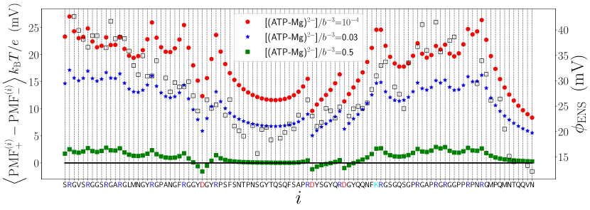
Fig. S4: FTS-predicted residue-specific, ATP-dependent effective electrostatic potentials of Caprin1. Test charges of extremely small concentration [tp] = [tn] $=10^{-5}b^{-3}$ are used to compute the spatially-averaged difference in potentials of mean force $\langle{\rm PMF}^{(i)}_{+}-{\rm PMF}^{(i)}_{-}\rangle$ [Eq. (S46)] plotted with the multiplicative factor $k_{\rm B}T/e$ (color symbols for different [(ATP-Mg)^2-] as indicated) along the left vertical axis in units of millivolt (mV). The simulation results shown here are from the FTS model for Caprin1 with (ATP-Mg)^2-, Na⁺, and Cl^- described in Supplmentary Methods. As discussed above, one half of this residue position ($i$)-dependent quantity may be viewed as an estimate of the effective electrostatic potentials of Caprin1. Included for comparison are the experimental NMR-determined residue-specific near-surface electrostatic potentials ($\phi_{\rm ENS}$) for Caprin1 at zero ATP (open black squares, right vertical scale) from Fig. 2C of Toyama et al.,LewisPNAS2022 indicating a similarity in the trend of $i$-dependent variation with the FTS-predicted counterparts for [(ATP-Mg)^2-] $=10^{-4}b^{-3}$ (red symbols) and [(ATP-Mg)^2-] $=0.03b^{-3}$ (blue symbols). Note that all of our FTS results are for [(ATP-Mg)^2-] $>0$, and the decreasing trend of the FTS-predicted effective electrostatic potentials with increasing [(ATP-Mg)^2-] is consistent with the reported experimental trend in Fig. 2C of ref. S36.

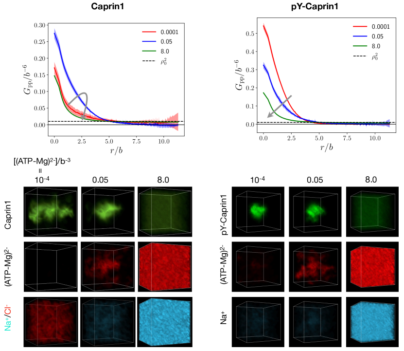
Fig. S6: Alternate FTS models for Caprin1 and pY-Caprin1 with (ATP-Mg)^2- and either Na⁺ or Cl^- (but not both) to maintain overall electric neutrality. For Caprin1, which has a net positive charge, (ATP-Mg)^2- is the counterion. Depending on [(ATP-Mg)^2-], either Cl^- is included as an additional counterion (when [(ATP-Mg)^2-] is insufficient to balance the positive charges on Caprin1), or Na⁺ is included as salt ion (when [(ATP-Mg)^2-] overcompensates the positive charges on Caprin1). Na⁺ and Cl^- are not included together in this simplified formulation. For pY-Caprin1, which has a net negative charge, Na⁺ is used as counterion, and its concentration depends on [(ATP-Mg)^2-] in such a way that electric neutrality of the entire system is maintained. Top panels: protein-protein correlation functions at different concentrations of (ATP-Mg)^2- (color coded in units of $b^{-3}$ as provided). Horizontal dashed lines are $(\rho^{0}_{\rm p})^{2}$ baselines as in Supplementary Fig. S5a,b. Grey arrows indicate increasing [(ATP-Mg)^2-]. Bottom panels: Field snapshots for system components at different [(ATP-Mg)^2-] (as indicated) for the Caprin1 (left panels) and pY-Caprin1 (right panels) systems. Results here are obtained at $l_{\rm B}=7b$. Details of the models are provided in Supplementary Methods.

References

References

- (1) Banani, S. F., Lee, H. O., Hyman, A. A. & Rosen, M. K. Biomolecular condensates: organizers of cellular biochemistry. Nat. Rev. Mol. Cell Biol. 18, 285–298 (2017).
- (2) Shin, Y. & Brangwynne, C. P. Liquid phase condensation in cell physiology and disease. Science 357, eaaf4382 (2017).
- (3) Gomes, E. & Shorter, J. The molecular language of membraneless organelles. J. Biol. Chem. 294, 7115–7127 (2019).
- (4) Tsang, B., Pritišanac, I., Scherer, S. W., Moses, A. M. & Forman-Kay, J. D. Phase separation as a missing mechanism for interpretation of disease mutations. Cell 183, 1742–1756 (2020).
- (5) Lyon, A. S., Peeples, W. B. & Rosen, M. K. A framework for understanding the functions of biomolecular condensates across scales. Nat. Rev. Mol. Cell Biol. 22, 215–235 (2021).
- (6) Boeynaems, S., Alberti, S., Fawzi, N. L., Mittag, T., Polymenidou, M., Rousseau, F., Schymkowitz, J., Shorter, J., Wolozin, B., Van Den Bosch, L., Tompa, P. & Fuxreiter, M. Protein phase separation: a new phase in cell biology. Trends Cell Biol. 28, 420–435 (2018).
- (7) Muiznieks, L. D., Sharpe, S., Pomès, R. & Keeley, F. W. Role of liquid-liquid phase separation in assembly of elastin and other extracellular matrix proteins. J. Mol. Biol. 430, 4741–4753 (2018).
- (8) Cinar, H., Fetahaj, Z., Cinar, S., Vernon, R. M., Chan, H. S. & Winter, R. Temperature, hydrostatic pressure, and osmolyte effects on liquid-liquid phase separation in protein condensates: Physical chemistry and biological implications. Chem. Eur. J. 25, 13049–13069 (2019).
- (9) Perry, S. L. Phase separation: Bridging polymer physics and biology. Curr. Opin. Colloid Interface Sci. 39, 86–97 (2019).
- (10) Dignon, G. L., Zheng, W. & Mittal, J. Simulation methods for liquid-liquid phase separation of disordered proteins. Curr. Opin. Chem. Eng. 23, 92–98 (2019).
- (11) Alberti, S., Gladfelter, A. & Mittag, T. Considerations and challenges in studying liquid-liquid phase separation and biomolecular condensates. Cell 176, 419–434 (2019).
- (12) Bremer, A., Farag, M., Borcherds, W. M., Peran, I., Martin, E. W., Pappu, R. V., Mittag, T. Deciphering how naturally occurring sequence features impact the phase behaviours of disordered prion-like domains. Nat. Chem. 14, 196–207 (2022).
- (13) Kato, M. & McKnight, S. L. A solid-state conceptualization of information transfer from gene to message to protein. Annu. Rev. Biochem. 87, 351-390 (2018).
- (14) McSwiggen, D. T., Mir, M., Darzacq, X. & Tjian, R. Evaluating phase separation in live cells: Diagnosis, caveats, and functional consequences. Genes Dev. 33, 1619–1634 (2019).
- (15) Wurtz, J. D. & Lee, C. F. Stress granule formation via ATP depletion-triggered phase separation. New J. Phys. 20, 045008 (2018).
- (16) Harmon, T. S., Holehouse, A. S., Rosen, M. K. & Pappu, R. V. Intrinsically disordered linkers determine the interplay between phase separation and gelation in multivalent proteins. eLife 6, e30294 (2017).
- (17) Lin, Y.-H., Forman-Kay, J. D. & Chan, H. S. Theories for sequence-dependent phase behaviors of biomolecular condensates. Biochemistry 57, 2499–2508 (2018).
- (18) Mittag, T. & Pappu, R. V. A conceptual framework for understanding phase separation and addressing open questions and challenges. Mol. Cell 82, 2201–2214 (2022).
- (19) Shen, Z., Jia, B., Xu, Y., Wessén, J., Pal, T., Chan, H. S., Du, S. & Zhang, M. Biological condensates form percolated networks with molecular motion properties distinctly different from dilute solutions. eLife 12, 81907 (2023).
- (20) Pappu, R. V., Cohen, S. R., Dar, F., Farag, M. & Kar, M. Phase transitions of associative biomacromolecules. Chem Rev. https://doi.org/10.1021/acs.chemrev.2c00814 (2023).
- (21) Lin, Y.-H., Wu, H., Jia, B., Zhang, M. & Chan, H. S. Assembly of model postsynaptic densities involves interactions auxiliary to stoichiometric binding. Biophys. J. 121, 157–171 (2022).
- (22) Nott, T. J., Petsalaki, E., Farber, P., Jervis, D., Fussner, E., Plochowietz, A., Craggs, T. D., Bazett-Jones, D. P., Pawson, T., Forman-Kay, J. D. & Baldwin, A. J. Phase transition of a disordered nuage protein generates environmentally responsive membraneless organelles. Mol. Cell 57, 936–947 (2015).
- (23) Lin, Y.-H., Forman-Kay, J. D. & Chan, H. S. Sequence-specific polyampholyte phase separation in membraneless organelles. Phys. Rev. Lett. 117, 178101 (2016).
- (24) Wang, J., Choi, J.-M., Holehouse, A. S., Lee, H. O., Zhang, X., Jahnel, M., Maharana, S., Lemaitre, R., Pozniakovsky, A., Drechsel, D., Poser, I., Pappu, R. V., Alberti, S., Hyman, A. A. A molecular grammar governing the driving forces for phase separation of prion-like RNA binding proteins. Cell 174, 688–699 (2018).
- (25) Vernon, R. M., Chong, P. A., Tsang, B., Kim, T. H., Bah, A., Farber, P., Lin, H. & Forman-Kay, J. D. Pi-Pi contacts are an overlooked protein feature relevant to phase separation. eLife 7, e31486 (2018).
- (26) Dignon, G. L., Zheng, W., Kim, Y. C. & Mittal, J. Temperature-controlled liquid-liquid phase separation of disordered proteins. ACS Cent. Sci. 5, 821–830 (2019).
- (27) Cinar, H., Cinar, S., Chan, H. S. & Winter, R. Pressure-induced dissolution and reentrant formation of condensed, liquid-liquid phase-separated elastomeric -elastin. Chem. Eur. J. 24, 8286–8291 (2018).
- (28) Cinar, H., Oliva, R., Lin, Y.-H., Chen, X., Zhang, M., Chan, H. S. & Winter, R. Pressure sensitivity of SynGAP/PSD-95 condensates as a model for postsynaptic densities and its biophysical and neurological ramifications. Chem. Eur. J. 26,11024–11031 (2020).
- (29) Cinar, S., Cinar, H., Chan, H. S. & Winter, R. Pressure-sensitive and osmolyte-modulated liquid-liquid phase separation of eye-lens -crystallins. J. Am. Chem. Soc. 141, 7347–7354 (2019).
- (30) Feric, M., Vaidya, N., Harmon, T. S., Mitrea, D. M., Zhu, L., Richardson, T. M., Kriwacki, R. W., Pappu, R. V. & Brangwynne, C. P. Coexisting liquid phases underlie nucleolar subcompartments. Cell 165, 1686–1697 (2016).
- (31) Maharana, S., Wang, J., Papadopoulos, D. K., Richter, D., Pozniakovsky, A., Poser, I., Bickle, M., Rizk, S., Guillén-Boixet, J., Franzmann, T. M., Jahnel, M., Marrone, L., Chang, Y. T., Sterneckert, J., Tomancak, P., Hyman, A. A. & Alberti, S. RNA buffers the phase separation behavior of prion-like RNA binding proteins. Science 360, 918–921 (2018).
- (32) Tsang, B., Arsenault, J., Vernon, R. M., Lin, H., Sonenberg, N., Wang, L. Y., Bah, A. & Forman-Kay, J. D. Phosphoregulated FMRP phase separation models activity-dependent translation through bidirectional control of mRNA granule formation. Proc. Natl. Acad. Sci. U.S.A. 116, 4218–4227 (2019).
- (33) Dutagaci, B., Nawrocki, G., Goodluck, J., Ashkarran, A. A., Hoogstraten, C. G., Lapidus, L. J. & Feig, M. Charge-driven condensation of RNA and proteins suggests broad role of phase separation in cytoplasmic environments. eLife 10, e64004 (2021).
- (34) Laghmach, R., Alshareedah, I., Pham, M., Raju, M., Banerjee, P. R. & Potoyan, D. A. RNA chain length and stoichiometry govern surface tension and stability of protein-RNA condensates. iScience 25, 104105 (2022).
- (35) Wang, Y., Lomakin, A., Kanai, S., Alex, R. & Benedek, G. B. Liquid–Liquid Phase Separation in Oligomeric Peptide Solutions. Langmuir 33, 7715-7721 (2017).
- (36) Owen, I. & Shewmaker, F. The role of post-translational modifications in the phase transitions of intrinsically disordered proteins. Int. J. Mol. Sci. 20, 5501 (2019).
- (37) Kim, T. H., Tsang, B., Vernon, R. M., Sonenberg, N., Kay, L. E. & Forman-Kay, J. D. Phospho-dependent phase separation of FMRP and CAPRIN1 recapitulates regulation of translation and deadenylation. Science 365, 825–829 (2019).
- (38) Snead, W. T. & Gladfelter, A. S. The control centers of biomolecular phase separation: how membrane surfaces, PTMs, and active processes regulate condensation. Mol. Cell 76, 295–305 (2019).
- (39) Nosella, M. L., Tereshchenko, M., Pritišanac, I., Chong, P. A., Toretsky, J. A., Lee, H. O. & Forman-Kay, J. D. O-linked- N-acetylglucosaminylation of the RNA-binding protein EWS N-terminal low complexity region reduces phase separation and enhances condensate dynamics. J. Am. Chem. Soc. 143, 11520–11534 (2021).
- (40) Marsh, J. A., Teichmann, S. A. & Forman-Kay, J. D. Probing the diverse landscape of protein flexibility and binding. Curr. Opin. Struct. Biol. 22, 643–650 (2012).
- (41) Song, J., Ng, S. C., Tompa, P., Lee, K. A. W. & Chan, H. S. Polycation- interactions are a driving force for molecular recognition by an intrinsically disordered oncoprotein family PLoS Comput. Biol. 9, e1003239 (2013).
- (42) Brangwynne, C. P., Tompa, P. & Pappu, R. V. Polymer physics of intracellular phase transitions. Nat. Phys. 11, 899–904 (2015).
- (43) Chen, T., Song, J. & Chan, H. S. Theoretical perspectives on nonnative interactions and intrinsic disorder in protein folding and binding. Curr. Opin. Struct. Biol. 30, 32–42 (2015).
- (44) Wang, Y., Zhou, H., Sun, X., Huang, Q., Li, S., Liu, Z., Zhang, C. & Lai, L. Charge segregation in the intrinsically disordered region governs VRN1 and DNA liquid-like phase separation robustness. J. Mol. Biol. 433, 167269 (2021).
- (45) Miyagi, T., Yamazaki, R., Ueda, K., Narumi, S., Hayamizu, Y., Uji-I, H., Kuroda, M. & Kanekura, K. The patterning and proportion of charged residues in the arginine-rich mixed-charge domain determine the membrane-less organelle targeted by the protein. Int. J. Mol. Sci. 23, 7658 (2022).
- (46) Galvanetto, N., Ivanović, M. T., Chowdhury, A., Sottini, A., Nüesch, M. F., Nettels, D., Best, R. B. & Schuler, B. Ultrafast molecular dynamics observed within a dense protein condensate. bioRiv https://doi.org/10.1101/2022.12.12.520135 (2022)
- (47) Das, R. K. & Pappu, R. V. Conformations of intrinsically disordered proteins are influenced by linear sequence distributions of oppositely charged residues. Proc. Natl. Acad. Sci. U.S.A. 110, 13392–13397 (2013).
- (48) Sawle, L. & Ghosh, K. A theoretical method to compute sequence dependent configurational properties in charged polymers and proteins. J. Chem. Phys. 143, 085101 (2015).
- (49) Chang, L.-W., Lytle, T. K., Radhakrishna, M., Madinya, J. J., Vélez, J., Sing, C. E. & Perry, S. L. Sequence and entropy-based control of complex coacervates. Nat. Comm. 8, 1273 (2017).
- (50) Amin, A. N., Lin, Y.-H., Das, S. & Chan, H. S. Analytical theory for sequence-specific binary fuzzy complexes of charged intrinsically disordered proteins. J. Phys. Chem. B 124, 6709–6720 (2020).
- (51) Lyons, H., Veettil, R. T., Pradhan, R., Fornero, C., De La Cruz, N., Ito, K., Eppert, M., Roeder, R. G. & Sabari1, B. R. Functional partitioning of transcriptional regulators by patterned charge blocks. Cell 186, 327–345 (2023).
- (52) Banerjee, P. R., Milin, A. N., Moosa, M. M., Onuchic, P. L. & Deniz, A. A. Reentrant phase transition drives dynamic substructure formation in ribonucleoprotein droplets. Agnew. Chem. Int. Ed. 56, 11354–11359 (2017).
- (53) Krainer, G., Welsh, T. J., Joseph, J. A., Espinosa, J. R., Wittmann, S., de Csilléry, E., Sridhar, A., Toprakcioglu, Z., Gudiškytė, G., Czekalska, M. A., Arter, W. E., Guillén-Boixet, J., Franzmann, T. M., Qamar, S., George-Hyslop, P. S., Hyman, A. A., Collepardo-Guevara, R., Alberti, S. & Knowles, T. P. J. Reentrant liquid condensate phase of proteins is stabilized by hydrophobic and non-ionic interactions. Nat. Comm. 12, 1085 (2021).
- (54) Hong, Y., Najafi, S., Casey, T., Shea, J.-E., Han, S. I. & Hwang, D. S. Hydrophobicity of arginine leads to reentrant liquid-liquid phase separation behaviors of arginine-rich proteins. Nat. Comm. 13 7326 (2022).
- (55) Alshareedah, I., Kaur, T., Ngo, J., Seppala, H., Kounatse, L. D., Wang, W., Moosa, M. M. & Banerjee, P. R. Interplay between short-range attraction and long-range repulsion controls reentrant liquid condensation of ribonucleoprotein-RNA complexes. J. Am. Chem. Soc. 141, 14593–14602 (2019).
- (56) Babinchak, W. M. et al. Small molecules as potent biphasic modulators of protein liquid-liquid phase separation. Nat. Comm. 11, 5574 (2020).
- (57) Hyman, A. A., Weber, C. A. & Jülicher, F. Liquid-liquid phase separation in biology. Annu. Rev. Cell Dev. Biol. 30, 39–58 (2014).
- (58) Bertrand, T. & Lee, C. F. Diversity of phase transitions and phase separations in active fluids. Phys. Rev. Res. 4, L022046 (2022).
- (59) Jain, S., Wheeler, J. R., Walters, R. W., Agrawal, A., Barsic, A. & Parker, R. ATPase-modulated stress granules contain a diverse proteome and substructure. Cell 164, 487–498 (2016).
- (60) Guilhas, B., Walter, J. C., Rech, J., David, G., Walliser, N. O., Palmeri, J., Mathieu-Demaziere, C., Parmeggiani, A., Bouet, J. Y., Le Gall, A. & Nollmann, M. ATP-driven separation of liquid phase condensates in bacteria. Mol. Cell 79, 293–303.e4 (2020).
- (61) Hayes, M. H., Peuchen, E. H., Dovichi, N. J., Weeks, D. L. Dual roles for ATP in the regulation of phase separated protein aggregates in Xenopus oocyte nucleoli. eLife 7, e35224 (2018).
- (62) Ghosh, A., Mazarakos, K. & Zhou, H.-X. Three archetypical classes of macromolecular regulators of protein liquid-liquid phase separation. Proc. Natl. Acad. Sci. U.S.A. 116, 19474–1948 (2019).
- (63) Ruff, K. M., Dar, F. & Pappu, R. V. Ligand effects on phase separation of multivalent macromolecules. Proc. Natl. Acad. Sci. U.S.A. 118, e2017184118 (2021).
- (64) Wright, R. H. G., Dily, F. L. & Beato, M. ATP, Mg2+, nuclear phase separation, and genome accessibility. Trends Biochem. Sci. 44, P565–574 (2019).
- (65) Booth, J. J., Omar, M., Abbott, S. & Shimizu, S. Hydrotrope accumulation around the drug: The driving force for solubilization and minimum hydrotrope concentration for nicotinamide and urea. Phys. Chem. Chem. Phys. 17, 8028–8037 (2015).
- (66) Martins, A. C., Benfica, J., Peréz-Sanchéz, G., Shimizu, S., Sintra, T. E., Schaeffer, N. & Coutinho, J. A. P. Assessing the hydrotropic effect in the presence of electrolytes: Competition between solute salting-out and salt-induced hydrotrope aggregation. Phys. Chem. Chem. Phys. 24, 21645–21654 (2022).
- (67) Patel, A. et al. Patel, A., Malinovska, L., Saha, S., Wang, J., Alberti, S., Krishnan, Y. & Hyman, A. A. ATP as a biological hydrotrope. Science 356, 753–756 (2017).
- (68) Tian, Z. & Qian, F. Adenosine triphosphate-induced rapid liquid-liquid phase separation of a model IgG1 mAb. Mol. Pharmaceutircs 18, 267–274 (2021).
- (69) Kang, J., Lim, L. & Song, J. ATP enhances at low concentrations but dissolves at high concentrations liquid-liquid phase separation (LLPS) of ALS/FTD-causing FUS. Biochem. Biophys. Res. Comm. 504, 545–551 (2018).
- (70) Kang, J., Lim, L., Lu, Y. & Song, J. A unified mechanism for LLPS of ALS-FTLD-causing FUS as well as its modulation by ATP and oligonucleic acids. PLoS Biol. 17, e3000327 (2019).
- (71) Dang, M., Lim, L., Kang, J. & Song, J. ATP biphasically modulates LLPS of TDP-43 PLD by specifically binding arginine residues. Comm. Biol. 4, 714 (2021).
- (72) Ren, C.-L., Shan, Y., Zhang, P., Ding, H.-M. & Ma, Y.-Q. Uncovering the molecular mechanism for dual effect of ATP on phase separation in FUS solution. Sci. Adv. 8, eabo7885 (2022).
- (73) Zhou, Q., Usluer, S., Zhang, F., Lenard, A. J., Bourgeois, B. M. R. & Madl, T. ATP regulates RNA-driven cold inducible RNA binding protein phase separation. Protein Sci. 30, 1438–1453 (2021).
- (74) Lin, Y.-H., Brady, J. P., Chan, H. S. & Ghosh, K. A unified analytical theory of heteropolymers for sequence-specific phase behaviors of polyelectrolytes and polyampholytes. J. Chem. Phys. 152, 045102 (2020).
- (75) Solomon, S., Xu, Y., Wang, B., David, M. D., Schubert, P., Kennedy, D. & Schrader, J. W. Distinct structural features of caprin-1 mediate its interaction with G3BP-1 and its induction of phosphorylation of eukaryotic translation initiation factor 2alpha, entry to cytoplasmic stress granules, and selective interaction with a subset of mRNAs. Mol. Cell. Biol. 27, 2324–2342 (2007).
- (76) Towers, E. R., Kelly, J. J., Sud, R., Gale, J. E. & Dawson, S. J. Caprin-1 is a target of the deafness gene Pou4f3 and is recruited to stress granules in cochlear hair cells in response to ototoxic damage. J. Cell Sci. 124, 1145–1155 (2011).
- (77) Kedersha, N., Panas, M. D., Achorn, C. A., Lyons, S., Tisdale, S., Hickman, T., Thomas, M., Lieberman, J., McInerney, G. M., Ivanov, P. & Anderson, P. G3BP-Caprin1-USP10 complexes mediate stress granule condensation and associate with 40S subunits. J. Cell Biol. 212, 845–860 (2016).
- (78) Vu, L., Ghosh, A., Tran, C., Tebung, W. A., Sidibé, H., Garcia-Mansfield, K., David-Dirgo, V., Sharma, R., Pirrotte, P., Bowser, R. & Vande Velde, C. Defining the Caprin-1 interactome in unstressed and stressed conditions. J. Proteome Res. 20, 3165–3178 (2021).
- (79) Song, D., Kuang, L., Yang, L., Wang, L., Li, H., Li, X., Zhu, Z., Shi, C., Zhu, H. & Gong, W. Yin and yang regulation of stress granules by Caprin-1. Proc. Natl. Acad. Sci. U.S.A. 119, e2207975119 (2022).
- (80) El Fatimy, R., Tremblay, S., Dury, A. Y., Solomon, S., De Koninck, P., Schrader, J. W. & Khandjian, E. W. Fragile X mental retardation protein interacts with the RNA-binding protein Caprin1 in neuronal RiboNucleoProtein complexes. PLoS ONE 7, e39338 (2012).
- (81) Ellis, J. A. & Luzio, J. P. Identification and characterization of a novel protein (p137) which transcytoses bidirectionally in Caco-2 cells. J. Biol.Chem. 270, 20717–20723 (1995).
- (82) Wang, B., David, M. D. & Schrader, J. W. Absence of Caprin-1 results in defects in cellular proliferation. J. Immunol. 175, 4274–4282 (2005).
- (83) Nakayama, K., Ohashi, R., Shinoda, Y., Yamazaki, M., Abe, M., Fujikawa, A., Shigenobu, S., Futatsugi, A., Noda, M., Mikoshiba, K., Furuichi, T., Sakimura, K. & Shiina, N. RNG105/caprin1, an RNA granule protein for dendritic mRNA localization, is essential for long-term memory formation. eLife 6, e29677 (2017).
- (84) Yang, T., Huang, L., Qin, H. & Mai, S. TRESS granule-associated RNA-binding protein CAPRIN1 drives cancer progression and regulates treatment response in nasopharyngeal carcinoma. Med. Oncol. 40, 47 (2022).
- (85) Pavinato, L., Delle Vedove, A., Carli, D., Ferrero, M., Carestiato, S., Howe, J. L., Agolini, E., Coviello, D. A., van de Laar, I., Au, P. Y. B., Di Gregorio, E., Fabbiani, A., Croci, S., Mencarelli, M. A., Bruno, L. P., Renieri, A., Veltra, D., Sofocleous, C., Faivre, L., Mazel, B., Safraou, H., Denommé-Pichon, A. S., van Slegtenhorst, M. A., Giesbertz, N., van Jaarsveld, R. H., Childers, A., Rogers, R. C., Novelli, A., De Rubeis, S., Buxbaum, J. D., Scherer, S. W., Ferrero, G. B., Wirth, B. & Brusco, A. CAPRIN1 haploinsufficiency causes a neurodevelopmental disorder with language impairment, ADHD and ASD. Brain, awac278, https://doi.org/10.1093/brain/awac278 (2022).
- (86) Wong, L. E., Kim, T. H., Muhandiram, D. R., Forman-Kay, J. D. & Kay, L. E. NMR experiments for studies of dilute and condensed protein phases: Application to the phase-separating protein CAPRIN1. J. Am. Chem. Soc. 142, 2471–2489 (2020).
- (87) Kim, T. H., Payliss, B. J., Nosella, M. L., Lee, I. T. W., Toyama, Y., Forman-Kay, J. D. & Kay, L. E. Interaction hot spots for phase separation revealed by NMR studies of a CAPRIN1 condensed phase. Proc. Natl. Acad. Sci. U.S.A. 118, e2104897118 (2021).
- (88) Toyama, Y., Rangadurai, A. K., Forman-Kay, J. D. & Kay, L. E. Mapping the per-residue surface electrostatic potential of CAPRIN1 along its phase-separation trajectory. Proc. Natl. Acad. Sci. U.S.A. 119, e2210492119 (2022).
- (89) Hornbeck, P. V., Zhang, B., Murray, B., Kornhauser, J. M., Latham, V. & Skrzypek, E. PhosphoSitePlus, 2014: mutations, PTMs and recalibrations. Nucl. Acids Res. 43, D512–520 (2015).
- (90) Monahan, Z., Ryan, V. H., Janke, A. M., Burke, K. A., Rhoads, S. N., Zerze, G. H., O’Meally, R., Dignon, G. L., Conicella, A. E., Zheng, W., Best, R. B., Cole, R. N., Mittal, J., Shewmaker, F. & Fawzi, N. L. Phosphorylation of the FUS low-complexity domain disrupts phase separation, aggregation, and toxicity. EMBO J. 36, 2951–2967 (2017).
- (91) Dignon, G. L., Zheng, W., Kim, Y. C., Best, R. B. & Mittal, J. Sequence determinants of protein phase behavior from a coarse-grained model. PLoS Comput. Biol. 14, e1005941 (2018).
- (92) Dignon, G. L., Best, R. B. & Mittal, J. Biomolecular phase separation: From molecular driving forces to macroscopic properties. Annu. Rev. Phys. Chem. 71, 53–75 (2020).
- (93) Carlson, C. R., Asfaha, J. B., Ghent, C. M., Howard, C. J., Hartooni, N., Safari, M., Frankel, A. D. & Morgan, D. O. Phosphoregulation of phase separation by the SARS-CoV-2 N protein suggests a biophysical basis for its dual functions. Mol. Cell 80, 1092-1103.e4 (2020).
- (94) Das, S., Eisen, A., Lin, Y.-H. & Chan, H. S. A lattice model of charge-pattern-dependent polyampholyte phase separation. J. Phys. Chem. B 122, 5418–5431 (2018).
- (95) McCarty, J., Delaney, K. T., Danielsen, S. P. O., Fredrickson, G. H. & Shea, J.-E. Complete phase diagram for liquid-liquid phase separation of intrinsically disordered proteins. J. Phys. Chem. Lett. 10, 1644–1652 (2019).
- (96) Danielsen, S. P. O., McCarty, I., Shea, J.-E., Delaney, K. T. & Fredrickson, G. H. Small ion effects on self-coacervation phenomena in block polyampholytes. J. Chem. Phys. 151, 034904 (2019).
- (97) Choi, J.-M., Dar, F. & Pappu, R. V. LASSI: A lattice model for simulating phase transitions of multivalent proteins. PLoS Comput. Biol. 15, e1007028 (2019).
- (98) Das, S., Lin, Y.-H., Vernon, R. M., Forman-Kay, J. D. & Chan, H. S. Comparative roles of charge, , and hydrophobic interactions in sequence-dependent phase separation of intrinsically disordered proteins. Proc. Natl. Acad. Sci. U.S.A. 117, 28795–28805 (2020).
- (99) Hazra, M. K. & Levy, Y. Charge pattern affects the structure and dynamics of polyampholyte condensates. Phys. Chem. Chem. Phys. 22, 19368–19375 (2020).
- (100) Joseph, J. A., Reinhardt, A., Aguirre, A., Chew, P. Y., Russell, K. O., Espinosa, J. R., Garaizar, A. & Collepardo-Guevara, R. Physics-driven coarse-grained model for biomolecular phase separation with near-quantitative accuracy. Nat. Comput. Sci. 1, 732–743 (2021).
- (101) Lin, Y.-H., Wessén, J., Pal, T., Das, S. & Chan, H.S. Numerical techniques for applications of analytical theories to sequence-dependent phase separations of intrinsically disordered proteins, in Phase-Separated Biomolecular Condensates, Methods and Protocols; Methods in Molecular Biology 2563 (eds. Zhou, H.-X., Spille, J.-H. & Banerjee, P. R.) 51–94 (Humana Press, 2023).
- (102) Lin, Y. -H., Brady, J. P., Forman-Kay J. D. & Chan, H. S. Charge pattern matching as a ‘fuzzy’ mode of molecular recognition for the functional phase separations of intrinsically disordered proteins. New J. Phys. 19, 115003 (2017).
- (103) Wessén, J., Pal, T. & Chan, H. S. Field theory description of ion association in phase separation of polyampholytes. J. Chem. Phys. 156, 194903 (2022).
- (104) Wessén, J., Das, S., Pal, T. & Chan, H. S. Analytical formulation and field-theoretic simulation of sequence-specific phase separation of proteinlike heteropolymers with short- and long-spatial-range interactions. J. Phys. Chem. B 126, 9222–9245 (2022). Correction: J. Phys. Chem. B 127, 11100 (2023).
- (105) Lin, Y.-H., Song, J., Forman-Kay, J. D. & Chan, H. S. Random-phase-approximation theory for sequence-dependent, biologically functional liquid-liquid phase separation of intrinsically disordered proteins. J. Mol. Liq. 228, 176–193 (2017).
- (106) Pal, T., Wessén, J., Das, S. & Chan, H. S. Subcompartmentalization of polyampholyte species in organelle-like condensates is promoted by charge-pattern mismatch and strong excluded-volume interaction. Phys. Rev. E 103, 042406 (2021).
- (107) Dobrynin, A. V. & Rubinstein, M. Theory of polyelectrolytes in solutions and at surfaces. Prog. Polym. Sci. 30, 1049–1118 (2005).
- (108) Lin, Y.-H. & Chan, H. S. Phase separation and single-chain compactness of charged disordered proteins are strongly correlated. Biophys. J. 112, 2043–2046 (2017).
- (109) Wessén, J., Pal, T., Das, S., Lin, Y.-H. & Chan, H. S. A simple explicit-solvent model of polyampholyte phase behaviors and its ramifications for dielectric effects in biomolecular condensates. J. Phys. Chem. B 125, 4337–4358 (2021).
- (110) Mahdi, K. A & Olvera de la Cruz, M. Phase diagrams of salt-free polyelectrolyte semidilute solutions. Macromolecules 33, 7649–7654 (2000).
- (111) Ermoshkin, A. V & Olvera de la Cruz, M. A modified random phase approximation of polyelectrolyte solutions. Macromolecules 36, 7824–7832 (2003).
- (112) Orkoulas, G., Kumar, S. K. & Panagiotopoulos, A. Z. Monte Carlo study of Coulombic criticality in polyelectrolytes. Phys. Rev. Lett. 90, 048303 (2003).
- (113) Muthukumar, M. 50th Anniversary perspective: A perspective on polyelectrolyte solutions. Macromolecules 50, 9528–9560 (2017).
- (114) Muthukumar, M. Double screening in polyelectrolyte solutions: Limiting laws and crossover formulas. J. Chem. Phys. 105, 5183–5199 (1996).
- (115) Budkov, Yu. A., Kolesnikov, A. L., Georgi, N., Nogovitsyn, E. A. & Kiselev, M. G. A new equation of state of a flexible-chain polyelectrolyte solution: Phase equilibria and osmotic pressure in the salt-free case. J. Chem. Phys., 142, 174901 (2015).
- (116) Shen, K. & Wang, Z.-G. Electrostatic correlations and the polyelectrolyte self energy. J. Chem. Phys., 146, 084901 (2017).
- (117) Shen, K. & Wang, Z.-G. Polyelectrolyte chain structure and solution phase behavior. Macromolecules 51, 1706–1717 (2018).
- (118) Eisenberg, H. & Mohan, G. R. Aqueous solutions of polyvinylsulfonic acid: Phase separation and specific interactions with ions, viscosity, conductance and potentiometry. J. Phys. Chem. 63, 671–680 (1959).
- (119) Moreira, A. G. & Netz, R. R. Phase behavior of three-component ionic fluids. Sur. Phys. J. D 13, 61–66 (2001).
- (120) Zhang, P., Alsaifi, N. M., Wu, J. & Wang, Z.-G. Salting-out and salting-in of polyelectrolyte solutions: A liquid-state theory study. Macromolecules 49, 9720–9730 (2016).
- (121) Silmore, K. S., Howard, M. P. & Panagiotopoulos, A. Z. Vapor-liquid phase equilibrium and surface tension of fully flexible Lennard-Jones chains. Mol. Phys. 115, 320–327 (2017).
- (122) Shimizu, S. & Chan, H. S. Configuration-dependent heat capacity of pairwise hydrophobic interactions. J. Am. Chem. Soc. 129, 2083–2084 (2001).
- (123) Regy, R. M., Thompson, J., Kim, Y. C. & Mittal, J. Improved coarse-grained model for studying sequence dependent phase separation of disordered proteins. Protein Sci. 30, 1371–1379 (2021).
- (124) Dannenhoffer-Lafage, T. & Best, R. B. A data-driven hydrophobicity scale for predicting liquid–liquid phase separation of proteins. J. Phys. Chem. B 125, 4046–4056 (2021).
- (125) Tesei, G., Schulze, T. K., Crehuet, R. & Lindorff-Larsen, K. Accurate model of liquid-liquid phase behavior of intrinsically disordered proteins from optimization of single-chain properties. Proc. Natl. Acad. Sci. U.S.A. 118, e2111696118 (2021).
- (126) Kim, Y. C. & Hummer, G. Coarse-grained models for simulations of multiprotein complexes: Application to ubiquitin binding. J. Mol. Biol. 375, 1416–1433 (2008).
- (127) Miyazawa, S. & Jernigan, R. L. Residue-residue potentials with a favourable contact pair term and an unfavourable high packing density term, for simulation and threading. J. Mol. Biol. 256, 623–644 (1996).
- (128) Zheng, W., Dignon, G. L., Jovic, N., Xu, X., Regy, R. M., Fawzi, N. L., Kim, Y. C., Best, R. B. & Mittal, J. Molecular details of protein condensates probed by microsecond long atomistic simulations. J. Phys. Chem. B 124, 11671–11679 (2020).
- (129) Brady, J. P., Farber, P. J., Sekhar, A., Lin, Y.-H., Huang, R., Bah, A. Nott, T. J., Chan, H. S., Baldwin, A. J., Forman-Kay, J. D. & Kay, L. E. Structural and hydrodynamic properties of an intrinsically disordered region of a germ cell-specific protein on phase separation. Proc. Natl. Acad. Sci. U.S.A. 114, E8194–E8203 (2017).
- (130) Fredrickson, G. H. The Equilibrium Theory Of Inhomogeneous Polymers; Oxford University Press Inc.:New York, 2006.
- (131) Parisi, G. On complex probabilities. Phys. Lett. B 131, 393–395 (1983).
- (132) Klauder, J. R. A Langevin approach to fermion and quantum spin correlation functions. J. Phys. A: Math. Gen. 16, L317–L319 (1983).
- (133) Parisi, G. & Wu, Y.-S. Perturbation theory without gauge fixing. Scientia Sinica 24, 483–496 (1981).
- (134) Chan, H. S. & Halpern, M. B. New Ghost-free infrared-soft gauges. Phys. Rev. D 33, 540–547 (1986).
- (135) Fredrickson, G. H., Ganesan, V. & Drolet, F. Field-theoretic computer simulation methods for polymers and complex fluids. Macromolecules 35, 16–39 (2002).
- (136) Lin, Y., McCarty, J., Rauch, J. N., Delaney, K. T., Kosik, K. S., Fredrickson, G. H., Shea, J.-E. & Han, S. Narrow equilibrium window for complex coacervation of tau and RNA under cellular conditions. eLife 8, e42571 (2019).
- (137) Garaizar, A. & Espinosa, J. R. Salt dependent phase behavior of intrinsically disordered proteins from a coarse-grained model with explicit water and ions. J. Chem. Phys. 155, 125103 (2021).
- (138) Jedlinska, Z. M. & Riggleman, R. A. The effect of monomer polarizability on the stability and salt partitioning in model coacervates. Soft Matter (2023) DOI: 10.1039/D3SM00706E
- (139) Wang, Q. & Schlenoff, J. B. The polyelectrolyte complex/coacervate continuum. Macromolecules 47, 3108–3116 (2014).
- (140) Hazra, M. & Levy, Y. Cross-talk of cation- interactions with electrostatic and aromatic interactions: A salt-dependent trade-off in biomolecular condensates. J. Phys. Chem. Lett. , (2023). ?? [Not yet available publicly]
- (141) Kim, S., Yoo, H. Y., Huang, J., Lee, Y., Park, S., Park, Y., Jin, S., Jung, Y. M., Zeng, H., Hwang, D. S. & Jho, Y. Salt triggers the simple coacervation of an underwater adhesive when cations meet aromatic electrons in seawater. ACS Nano 11, 6764–6772 (2017).
- (142) Wadsworth, G. M., Zahurancik, W. J., Zeng, X., Pullara, P., Lai, L. B., Sidharthan, V., Pappu, R. V., Gopalan, V. & Banerjee, P. R. RNAs undergo phase transitions with lower critical solution temperatures. Nat. Chem. DOI: https://doi.org/10.1038/s41557-023-01353-4 (2023).
- (143) Morishita, K., Watanabe, K., Naguro, I. & Ichijo, H. Sodium ion influx regulates liquidity of biomolecular condensates in hyperosmotic stress response. Cell Rep. 42, 112315 (2023).
- (144) Fetahaj, Z., Ostermeier, L., Cinar, H., Oliva, R. & Winter, R. Biomolecular condensates under extreme Martian salt conditions. J. Am. Chem. Soc. 143, 5247–5259 (2021).
- (145) Tesei, G., Vazdar, M., Jensen, M. R., Cragnell, C., Mason, P. E., Heyda, J. Skepö, M., Jungwirth, P. & Lund, M. Self-association of a highly charged arginine-rich cell-penetrating peptide. Proc. Natl. Acad. Sci. U.S.A. 114, 11428–11433 (2017).
- (146) Liu, B. R., Chiou, S.-H., Huang, Y.-W. & Lee, H.-J. Bio-membrane internalization mechanisms of arginine-rich cell-penetrating peptides in various species. Membranes (Basel) 12, 88 (2022).
- (147) Radhakrishna M., Basu K., Liu Y. L., Shamsi R., Perry S. L. & Sing C. E. Molecular connectivity and correlation effects on polymer coacervation. Macromolecules 50, 3030– (2017).
- (148) Li, L., Srivastava, S., Andreev, M., . Marciel, A. B., de Pablo, J. J. & Tirrell, M. V. Phase behavior and salt partitioning in polyelectrolyte complex coacervates. Marcomolecules 51, 2988–2995 (2018).
- (149) Herrera, S. E., Agazzi, M. L., Apuzzo, E., Cortez, M. L., Marmisollé, W. A., Tagliazucchi, M. & Azzaroni, O. Polyelectrolyte-multivalent molecule complexes: physicochemical properties and applications. Soft Matter 19, 2013–2041 (2023).
- (150) Qian, D., Welsh, T. J., Erkamp, N. A., Qamar, S., Nixon-Abell, J., Krainer, G., St. George-Hyslop, P., Michaels, T. C. T. & Knowles, T. P. J. Tie-Line analysis reveals interactions driving heteromolecular condensate formation. Phys. Rev. X 12, 041038 (2022).
- (151) Belloni, L., Olvera de la Cruz, M., Delsanti, M., Dalbiez, J. P., Spalla, O. & Drifford, M. Polyelectrolyte solutions + multivalent salts = phase separation. Il Nuovo Cimento 16, 727–736 (1994).
- (152) Olvera de la Cruz, M., Belloni, L., Delsanti, M., Dalbiez, J. P., Spalla, O. & Drifford, M. Precipitation of highly charged polyelectrolyte solutions in the presence of multivalent salts. J. Chem. Phys. 103, 5781–5791 (1995).
- (153) Lenton, S., Hervø-Hansen, S., Popov, A. M., Tully, M. D., Lund, M. & Skepö, M. Impact of arginine-phosphate interactions on the reentrant condensation of disordered proteins. Biomacromolecules 22, 1532–1544 (2021).
- (154) Crabtree, M. D., Holland, J., Pillai, A. S., Kimpella, P. S., Babl, L., Turner, N. N., Eaton, J. T., Hochberg, G. K. A., Aarts, D. G. A. L., Redfield, C., Baldwin, A. J. & Nott, T. J. Ion binding with charge inversion combined with screening modulates DEAD box helicase phase transitions. Cell Rep. 42, 113375 (2023).
- (155) Nakashima, K. K., Baaij, J. F. & Spruijt, E. Reversible generation of coacervate droplets in an enzymatic network. Soft Matter 14, 361–367 (2018).
- (156) Kota, D., Prasad, R. & Zhou, H.-X. ATP mediates phase separation of disordered basic proteins by bridging intermolecular interaction networks. BioRxiv DOI: 10.1101/2023.08.20.554035 (2023)
- (157) Saurabh, S., Chong, T. N., Bayas, C., Dahlberg, P. D., Cartwright, H. N., Moerner, W. E. & Shapiro, L. ATP-responsive biomolecular condensates tune bacterial kinase signaling. Sci. Adv. 8, eabm6570 (2022).
- (158) Yewdall, N. M., André, A. A. M., van Haren, M. H. I., Nelissen, F. H. T., Jonker, A. & Spruijt, E. ATP:Mg2+ shapes material properties of protein-RNA condensates and their partition of clients. Biophys. J. 121, 3962–3974 (2022).
- (159) Adhikari, S., Leaf, M. A. & Muthukumar, M. Polyelectrolyte complex coacervation by electrostatic dipolar interactions. J. Chem. Phys. 149, 163308 (2018).
- (160) Li, L., Rumyantsev, A. M., Srivastava, S., Meng, S., de Pablo, J. J. & Tirrell, M. V. Effect of solvent quality on the phase behavior of polyelectrolyte complexes. Marcomolecules 54, 105–114 (2021).
- (161) Ali, S., Bleuel, M. & Prabhu, V. M. Lower critical solution temperature in polyelectrolyte complex coacervates. ACS Marco Lett. 8, 289–293 (2019).
- (162) Wiesner, S., Wybenga-Groot, L. E., Warner, N., Lin, H., Pawson, T., Forman-Kay, J. D. & Sicheri, F. A change in conformational dynamics underlies the activation of Eph receptor tyrosine kinases. EMBO J. 25, 4686–4696 (2006).
- (163) Wang, Z.-G. Fluctuation in electrolyte solutions: The self energy. Phys. Rev. E 81, 021501 (2010).
- (164) Stratonovich, R. L. On a method of calculating quantum distribution functions. Soviet Physics Doklady 2, 416–419 (1958).
- (165) Hubbard, J. Calculation of partition functions. Phys. Rev. Lett. 3, 77–78 (1959).
- (166) Anderson, J. A., Glaser, J. & Glotzer, S. C. HOOMD-blue: A Python package for high-performance molecular dynamics and hard particle Monte Carlo simulations. Comput. Mater. Sci. 173, 109363 (2020).
- (167) Anderson, J. A., Lorenz, C. D. & Travesset, A. General purpose molecular dynamics simulations fully implemented on graphics processing units. J. Comput. Phys. 227, 5342–5359 (2008).
- (168) Dignon, G. L., Zheng, W. & Mittal, J. Simulation methods for liquid–liquid phase separation of disordered proteins. Curr. Opin. Chem. Eng. 23, 92–98 (2019).
- (169) Das, S., Amin, A. N., Lin, Y.-H. & Chan, H. S. Coarse-grained residue-based models of disordered protein condensates: Utility and limitations of simple charge pattern parameters. Phys. Chem. Chem. Phys. 20, 28558–28574 (2018).
- (170) Joung, I. S. & Cheatham, T. E. 3rd. Determination of alkali and halide monovalent ion parameters for use in explicitly solvated biomolecular simulations. J. Phys. Chem. B 112, 9020–9041 (2008).
- (171) Tros, M., Zheng, L., Hunger, J., Bonn, M., Bonn, D., Smits, G. J. & Woutersen, S. Picosecond orientational dynamics of water in living cells. Nat. Commun. 8, 904 (2017).
- (172) Martyna, G. J., Tobias, D. J. & Klein, M. L. Constant pressure molecular dynamics algorithms. J. Chem. Phys. 101, 4177–4189 (1994).
- (173) Tuckerman, M. E., Alejandre, J., López-Rendón, R., Jochim , A. L. & Martyna G. J. A Liouville-operator derived measure-preserving integrator for molecular dynamics simulations in the isothermal–isobaric ensemble. J. Phys. A: Math. Gen. 39, 5629–5651 (2006).
- (174) LeBard, D. N., Levine, B. G., Mertmann, P., Barr, S. A., Jusufi, A., Sanders, S., Klein, M. L. & Panagiotopoulos, A. Z. Self-assembly of coarse-grained ionic surfactants accelerated by graphics processing units. Soft Matter 8, 2385–2397 (2012).
- (175) Lennon, E. M., Mohler, G. O., Ceniceros, H. D., Garca-Cervera, C. J. & Fredrickson, G. H. Numerical solutions of the complex Langevin equations in polymer field theory. Multiscale Modeling & Simulation 6, 1347–1370 (2008).