Online Adaptive Data-driven State-of-health Estimation for Second-life Batteries with BIBO Stability Guarantees

Abstract

A key challenge that is currently hindering the widespread deployment and use of retired electric vehicle (EV) batteries for second-life (SL) applications is the ability to accurately estimate and monitor their state of health (SOH). Second-life battery systems can be sourced from different battery packs with lack of knowledge of their historical usage.

To facilitate the on-the-field use of SL batteries, this paper introduces an online adaptive health estimation strategy with guaranteed stability. This method relies exclusively on operational data that can be accessed in real time from SL batteries. The adaptation algorithm is designed to ensure bounded-input-bounded-output (BIBO) stability. The effectiveness of the proposed approach is shown on a laboratory aged experimental data set of retired EV batteries. The estimator gains are dynamically adapted to accommodate the distinct characteristics of each individual cell, making it a promising candidate for future SL battery management systems (BMS₂).

I Introduction

Accelerated adoption of lithium-ion battery (LIB) technology for various applications is pushing the transition towards sustainable energy. Electric vehicles (EVs) are at the forefront of this adoption [1, 2] with some OEMs announcing a complete shift towards EV production moving away from internal combustion engine (ICE) vehicles [3]. While this shift is much needed to address climate change concerns, naturally, this has also increased the pressure on the supply chain for the raw materials needed to manufacture LIBs [4]. To tackle the large demand of raw materials for battery manufacturing, and fully embrace a circular economy paradigm, one promising solution lies in the reuse of EV batteries once they retire from their first-life (FL). These batteries are expected to retain approximately 70-80% of their nominal capacity, and they could be well-suited for stationary applications such as grid storage, power generation, and end-user services e.g., uninterrupted power supply (UPS) [5].

One challenge of working with second-life (SL) batteries is to identify accurately their actual state-of-health (SOH) since these batteries are obtained from different battery packs which means they have gone through different levels of usage. Due to the heterogeneity of the cells in these packs, ensuring safe usage of refurbished batteries is paramount. For this, we propose a battery management system for SL batteries, referred to as BMS₂. BMS₂ is based on all the major hardware components of a conventional BMS; on the software side, BMS₂ still performs SOX estimation e.g., state-of-charge (SOC), using standard algorithms. In this work, though, we focus on the health estimation problem of retired EV batteries. The level of degradation of retired batteries is dependent on their usage history [6]; however, at present, historical data are not publicly available for any retired batteries [7]. With BMS₂, the idea is to overcome the lack of usage history by allowing the model to adapt to new incoming data to maintain accuracy on SOH estimation.

II Literature Review

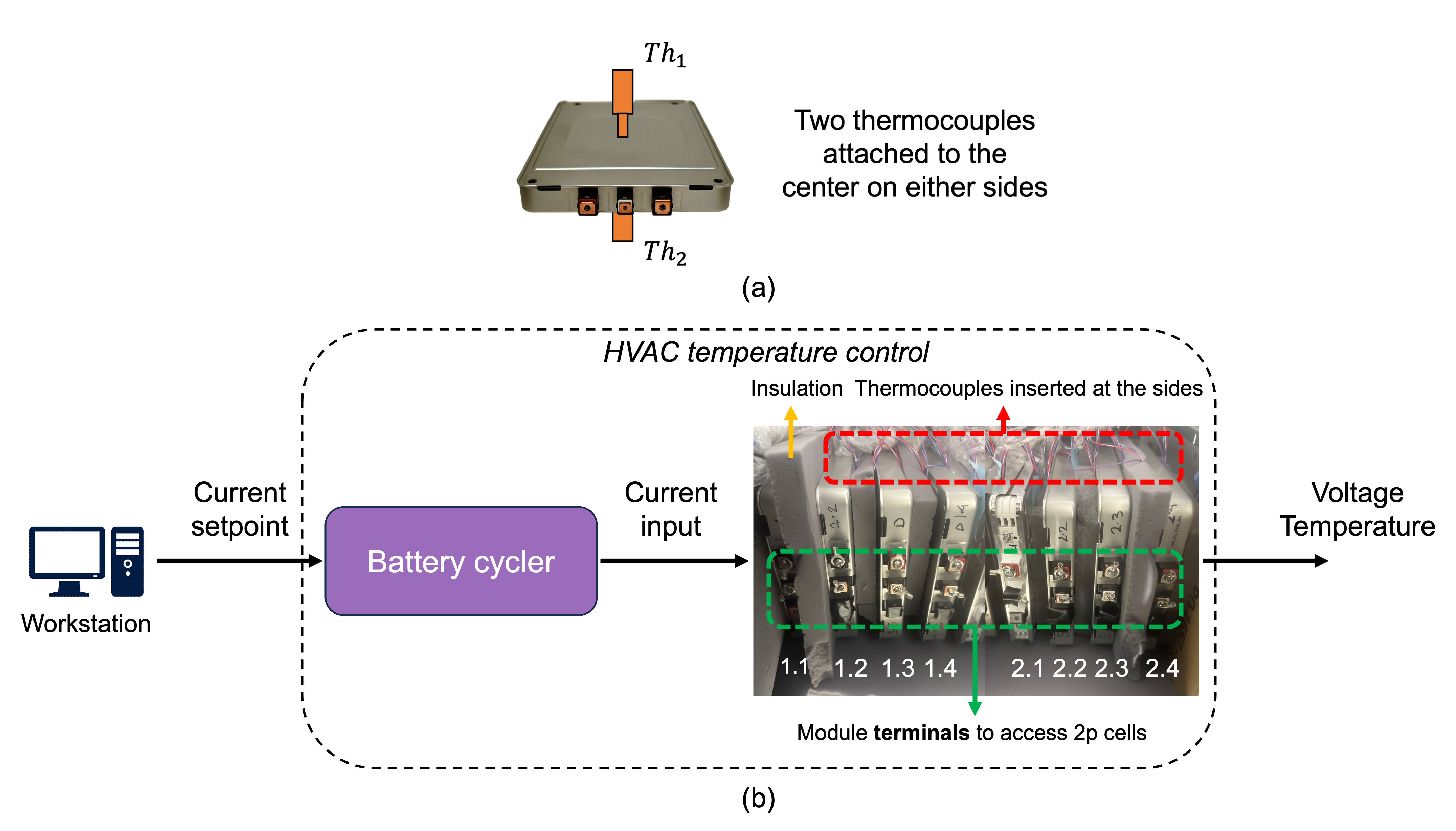
Figure 1: Experimental setup. (a) Schematic of the two thermocouples $Th_{1}$ and $Th_{2}$ attached on either sides of the module surface to measure the surface temperature. (b) Schematic of the experimental setup showing the battery cycler and eight modules. The modules have insulation between one another and the thermocouples can be going inserted into the sides of the modules. On the front, positive terminal is on the top, ground terminal in the middle, and negative terminal at the bottom. The workstation is used to set the current setpoint for the battery cycler, which inputs actual current into the modules, and voltage and temperature are measured at the output. The experimental setup is present inside an HVAC-controlled room located in Santa Clara, CA at Relyion Energy Inc HQs.

Numerous works exist that use either semi-empirical methods or physics-based models for SOH estimation [8]. The former performs well on simple, well-maintained laboratory conditions, but they are prone to accuracy loss when applied to on-the-field realistic conditions [8]; the latter is based on coupled-PDEs and provides a plethora of information about internal battery states. However, physics-based models are computationally intensive and a lot of parameters need to be identified [9]. For this work, we employ data-driven models that are capable of learning complex degradation trajectories from input data and the choice of the model can be adjusted based on the computational resources needed to run these models onboard. SOH estimation using data-driven models has used regression techniques such as Linear Regression [10], Support Vector Regression [11], Gaussian Process Regression [12]. Other works have also used neural networks [13, 14] that are widely regarded as universal function approximators. However, to achieve good performance on neural networks, a large dataset is required and a lot of hyperparameter tuning is needed.

While these data-driven techniques have proved useful, they are limited by the kind of training data that is used. Traditionally, the performance of these models tends to deteriorate if the incoming data is out-of-distribution (OOD) [15] meaning that it is statistically different from the kind of data that was used to train the model. Existing work around adaptive estimation utilizes periodic stream of health indicators by performing reference performance tests (RPTs) and using feedback to update the model [16, 17, 18, 19]. Evidently, this is infeasible for BMS₂ since SL batteries cannot be continuously disengaged once they are deployed [20]. Another popular approach adopted for this problem uses transfer learning in which a baseline model is trained using a neural network. Afterwards, the initial layers of the model are frozen while the final few layers are retrained on the target domain data [21, 22, 23, 24]. The limitation of transfer learning resides in the target domain used to re-train the model. In field operation, the uncertainty of the incoming data is high and it is difficult to ensure that the model performs consistently.

The health estimation of BMS₂ not only requires online functionality but also demands adaptability. This implies that the estimator model should dynamically adjust and evolve as it gathers more and more online measurements. In principal, it should enhance the model’s generalizability to various operating conditions and unforeseen SL batteries once they are deployed. Moreover, taking into account the auto-correlation of battery SOH aging as a time series [25], historical health data gains significance in the estimation of the current SOH. From a practical standpoint, as information is pushed in, it becomes essential for health estimator to guarantee the error to stay within specified bounds. Nonetheless, there is a dearth of literature providing mathematical assurances for these boundaries.

To overcome the uncertainty associated with SOH estimation algorithms trained offline, in this work, we introduce an adaptive SOH estimation method that combines clustering-based estimation with regression-based estimation. Since adaptive SOH estimation is based on the online stream of incoming data, it is pertinent to ensure that the model estimation remains bounded. To this end, the stability of the adaptive framework is theoretically provided via bounded-input bounded-output (BIBO) stability. We compare the results obtained from the adaptive framework with the results obtained from the offline model to show our model adaptation improves the estimation accuracy.
Notation: The following notation is used in the paper:

• Sequence $\{a_{n}\}_{n\leq N}\triangleq\{a_{1},a_{2},\cdots,a_{N}\}$ where $a_{n}$ represents the general item of the sequence $\{a_{n}\}$, and $N$ represents the length of the sequence. For ease of notation, if not specified, $\{a_{n}\}$ is equivalent to $\{a_{n}\}_{n\leq N}$.

• $\|\cdot\|_{2}$ represents the $\mathcal{L}^{2}$ norm. The $\mathcal{L}^{2}$ norm of a sequence $\{x_{n}\}=(x_{1},x_{2},\cdots,x_{N})$ is captured by the formula $\|\{x_{n}\}\|_{2}=\sqrt{\sum_{n=1}^{N}x_{n}^{2}}$.

• $\|\cdot\|$ represents the $\mathcal{L}^{\infty}$ norm. The $\mathcal{L}^{\infty}$ norm of a sequence $\{x_{n}\}=(x_{1},x_{2},\cdots,x_{N})$ is captured by the formula $\|\{x_{n}\}\|_{\infty}=\max_{n=1}^{N}\left|x_{n}\right|$.

• $\mathbb{R}^{+}=\{z\in\mathbb{R}\mathrel{\mathop{\mathchar 58\relax}}z>0\}$.

III Dataset

The dataset used in this work consists of eight retired pouch cells obtained from Nissan leaf EV battery packs with LMO/graphite chemistry. The nominal capacity (fresh cell) is 33.1 Ah and the voltage range is from 2.5 V to 4.2 V. The cells are arranged in modules where each module contains four pouch cells in a 2s2p configuration accessible via the three terminals outside the module. Based on the module design, a pair of terminals (must include the middle terminal) can be used to access 2p cells while positive and negative terminal together can be used to access the complete 2s2p configuration. In this work, we access only the 2p cells using the positive and middle terminals and refer to these 2p cells as a single cell for the remainder of this paper. Hence, the eight cells in the dataset are, in essence, eight 2p cells. Surface temperature of the cells is measured by a pair of thermocouples $Th_{1}$ and $Th_{2}$ attached to the side of all the modules. The complete experimental setup is shown in Fig. 1.

Since these are retired cells with an unknown usage history, it is important to characterize these cells to understand their existing SOH. Initially, an experimental campaign is designed which consists of three different reference performance tests (RPTs) and an aging profile repeated multiple times in between RPTs. The cycling profile is designed to mimic the load expected in a grid-storage application in a simplistic manner. The RPTs consists of C/20 capacity test, a Hybrid Pulse Power Characterization (HPPC) test, and a C/40 Open-circuit voltage (OCV). One important aspect of this experimental campaign is that, except for the OCV test performed between 2.5 and 4.2V, all the other tests are performed between 3V to 4V. This kind of voltage derating is well-suited for SL applications to guarantee safe operation by limiting the growth of solid electrolyte interphase (SEI) layer and thereby, reducing battery degradation [26]. The initial distribution of C/20 capacity of these cells is shown in Fig. 2. $Q_{init,ch,C/20}$ is the initial C/20 charge capacity and $Q_{init,dis,C/20}$ is the initial C/20 discharge capacity obtained from the charge and discharge portions of the C/20 test, respectively. A small difference between $Q_{init,ch,C/20}$ and $Q_{init,dis,C/20}$ indicates that these cells have high coulombic efficiency. Detailed information about the experimental campaign, including length of experimental campaign and design of testing protocols, is given in [27].

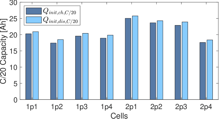
Figure 2: Initial distribution of C/20 capacity for all SL cells with a small difference between initial charge capacity $Q_{init,ch,C/20}$ and initial discharge capacity $Q_{init,dis,C/20}$. Cell 2.1 has the highest initial capacity while Cell 2.4 has the lowest initial capacity among all cells.

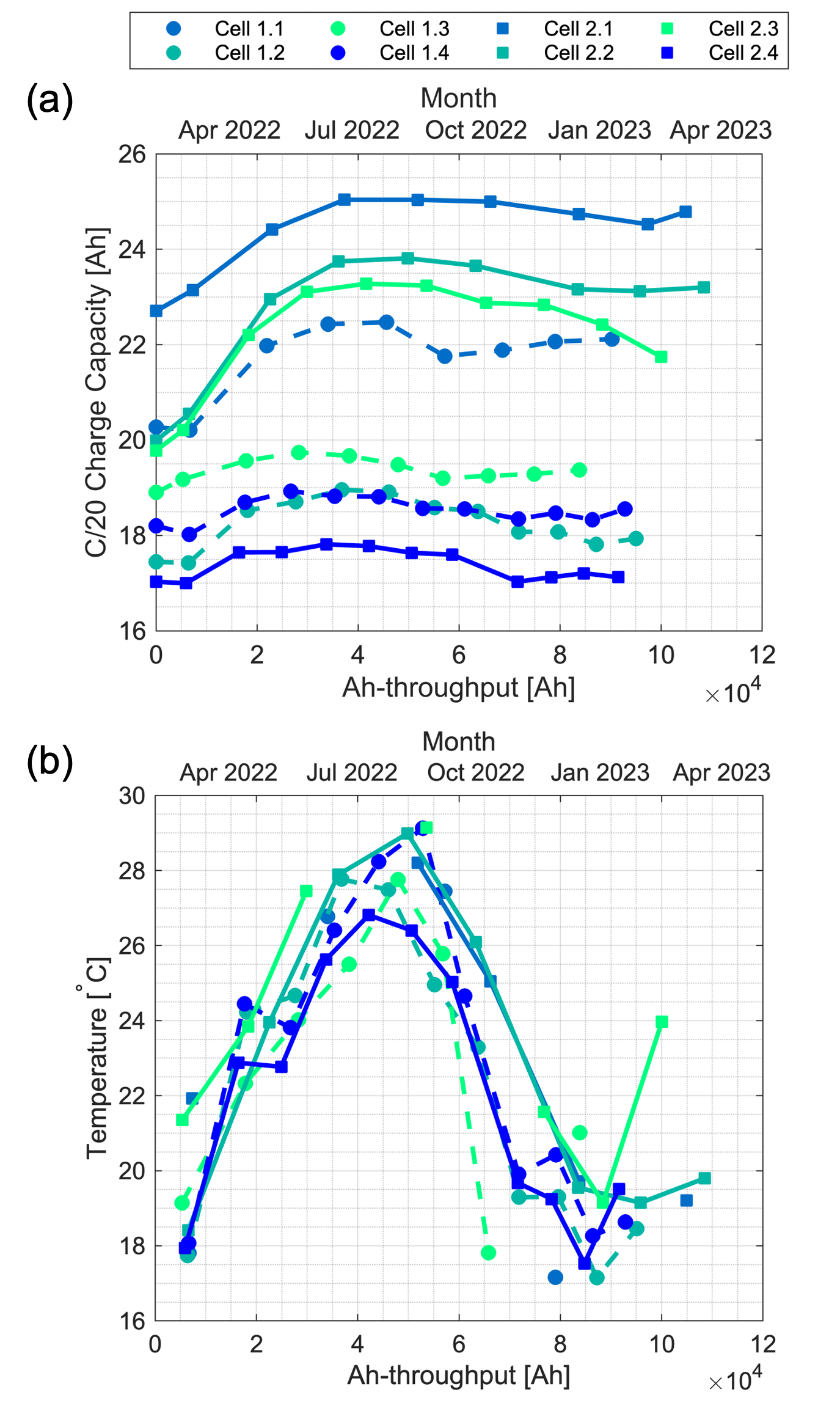
Figure 3: Capacity and temperature for the SL cells used in this work. (a) C/20 charge capacity as a function of Ah-throughput. (b) Temperature as a function of Ah-throughput (below) and months (above) with a parabolic shape reaching a maximum value during the months of August/September 2022 indicating the effect of seasonal variation of temperature on all the cells. Gaps in temperature lines represent missing data for those cells e.g., Cell 2.3.

For the pouch cells tested, the C/20 capacity trajectory is shown in Fig. 3(a). As opposed to conventional battery degradation profiles (linear, sub-linear, or super-linear) [28], these cells exhibit an increase in capacity with all cells reaching a maximum capacity point which is higher than their initial capacities. As outlined in detail in [27], this behavior is due to the varying temperature that the cells experience during the experimental campaign (see Fig. 3(b)). The dataset, being the first of its kind, highlights how cells can potentially behave when used in practical SL applications, especially in cases where the temperature cannot be controlled. Furthermore, the effect of voltage derating can be observed by the fact that cells, upon reaching the one-year mark from start of testing, still possess higher or equal capacity compared to their initial capacities.

IV Data-driven Model

The SOH for these SL batteries is the current C/20 capacity of these cells normalized by their initial C/20 capacity at the start of SL. For this work, an Elastic-net regression (ENR) model is selected which provides ease of training and adaptability as well as low computational requirements. The choice of data-driven model is dictated by the complexity of the data, computational resources, and the training time required to train these models. In our case, another factor that is taken into account is the ease of parameter adaptation when new data becomes available. Furthermore, since our dataset is small in terms of the number of cells, this model provides a suitable framework for the health estimation problem [27]. In ENR, the loss function used to train the model consists of a linear combination of $L_{1}$ (lasso) and $L_{2}$ (ridge) regularization terms. The following optimization problem is solved to train the model:

$$\hat{\beta}=\operatorname*{arg\,min}_{\beta_{0},\beta,\lambda}\,\,\|Y-X\beta-\beta_{0}\mathbf{1}_{n\times 1}\|_{2}+$$

$$\lambda\left(1-\alpha\right)\|\beta\|_{2}^{2}+\lambda\alpha\|\beta\|_{1}$$ (1)

where $Y\in\mathbb{R}^{n}$ represents the SOH indicators, $X\in\mathbb{R}^{n\times m}$ contains $m$ features each with $n$ observations, $\beta\in\mathbb{R}^{m}$ contains the regression coefficients, and $\beta_{0},\lambda,\alpha\in\mathbb{R}$ are the scaler intercept, the hyperparameter to adjust the influence of $L_{1}$ and $L_{2}$, and the regularization parameter, respectively.

Figure 4: ENR model with input features $X^{test}$ from the test set and an estimated scalar output $\hat{Q}^{test}_{ch,C/20}$ as a function of Ah-throughput.

IV-A Offline ENR

The output is chosen to be the C/20 charge capacity. It is noted that due to the high coulombic efficiency of the cells, the difference between charge and discharge capacity is minimal. Fig. 4 shows the flow of data through the offline ENR model where $X^{test}(Ah_{n})$ represents the input features of the test set at $Ah_{n}$ and $\hat{Q}^{test}_{ch,C/20}(Ah_{n})$ is the estimated C/20 charge capacity. More details about the input features are given in [27]. From a total of 8 cells, 6 cells are used for training and 2 cells are used for testing. The model is referred to as “offline” because the estimation results are based purely on the existing training data and no attempt is made to adapt the model to improve its estimation based on any new data. From a total of $n=8$ cells, the number of possible $r=2$ cell combinations comes out to be ${}_{8}C_{2}=28$ given by

$${}_{n}C_{r}=\frac{n!}{r!(n-r)!}$$ (2)

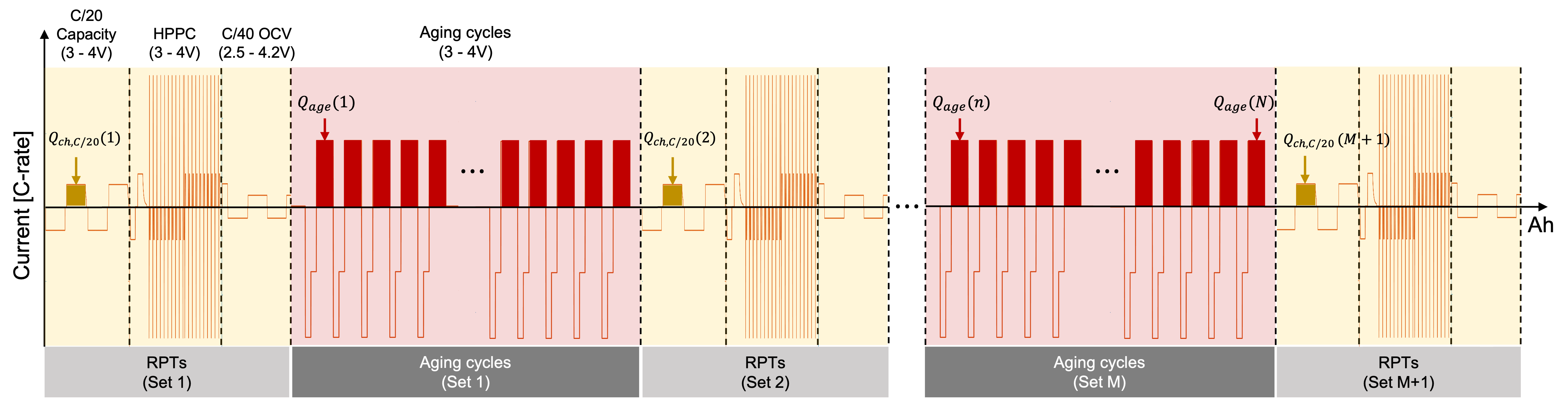
Figure 5: Design of experiments showing Reference performance tests (RPTs) and aging cycles. RPTs contain C/20 capacity test, HPPC test, and OCV test, which makes one set. For the complete campaign, $M$ sets of aging cycles are performed while $M+1$ sets of RPTs are performed. From C/20 capacity test, $Q_{ch,C/20}$ is obtained once for each RPT set and $Q_{age}$ is obtained from each cycle, which means $N>>M$ for the dataset. The limits of $Q_{ch,C/20}(i)$ are given by $t_{ch}^{C/20}(i)$ and $t_{dis}^{C/20}(i)$ where $i=1,2,...,M+1$, and the limits of $Q_{age}(j)$ are given by $t_{ch}^{age}(j)$ and $t_{dis}^{age}(j)$ where $j=1,2,...,n,...,N$.

The performance of the offline ENR model is quantified by the root-mean-squared-error (RMSE), root-mean-squared-percentage-error (RMSPE), and mean absolute error (MAE) which are given by:

$$\text{RMSE}=\sqrt{\frac{1}{M}\sum_{y\in Y,\;\hat{y}\in\hat{Y}}\left(\hat{y}-y\right)^{2}}\times 100\,\%$$ (3)

$$\text{RMSPE}=\sqrt{\frac{1}{M}\sum_{y\in Y,\;\hat{y}\in\hat{Y}}\left(\frac{\hat{y}-y}{y}\right)^{2}}\times 100\,\%$$ (4)

$$\text{MAPE}=\frac{1}{M}\sum_{y\in Y,\;\hat{y}\in\hat{Y}}\frac{\left|\hat{y}-y\right|}{y}\times 100\,\%$$ (5)

where $Y$ is the measured data, $\hat{Y}$ is the model estimation, and $M$ is the number of samples.

In Table I, the performance of offline ENR model for the different combination of the test sets is shown. The lowest test error is achieved by the test set (1.2, 2.1) with an RMSE of 0.28 Ah and an MAPE of 1%, and the estimation results are shown in Fig. 6(a). Apart from two cases, all the RMSE values are below 1 Ah which shows that the model has good performance. The worst performance is achieved on the test set (1.1, 2.3) with an RMSE of 1.495 Ah and an MAPE of 5.26%. This drop in performance is attributed to Cell 2.3 in which the input features exhibit uncharacteristic behaviors due to errors in data measurement. The absence of Cell 2.3 in the training set results in the poor performance of the model. This is also shown in Fig. 6(b) showing the worst case performance of the model with Cell 2.3 clearly having a larger error as compared to Cell 1.1.

TABLE I: Performance of offline ENR model

Test set	RMSE [Ah]	RMSPE [%]	MAPE [%]
(1.1, 1.2)	0.495699	2.451021	1.565399
(1.1, 1.3)	0.555976	2.769582	2.167772
(1.1, 1.4)	0.484275	2.394690	1.602038
(1.1, 2.1)	0.628837	2.920140	2.046725
(1.1, 2.2)	0.682332	3.193374	2.437554
(1.1, 2.3)	1.495901	6.595751	5.265551
(1.1, 2.4)	0.566506	2.915141	2.185236
(1.2, 1.3)	0.689619	3.713645	3.319282
(1.2, 1.4)	0.396715	2.147421	1.957864
(1.2, 2.1)	0.280542	1.218656	1.006326
(1.2, 2.2)	0.529458	2.538446	2.010231
(1.2, 2.3)	0.800931	3.533838	2.553109
(1.2, 2.4)	0.485609	2.734561	2.507264
(1.3, 1.4)	0.355872	1.892205	1.683591
(1.3, 2.1)	0.562813	2.580422	2.353598
(1.3, 2.2)	0.608824	2.832768	2.695224
(1.3, 2.3)	0.763585	2.400556	2.894587
(1.3, 2.4)	0.457407	2.533389	2.187910
(1.4, 2.1)	0.401952	1.827907	1.246798
(1.4, 2.2)	0.530269	2.527535	1.905807
(1.4, 2.3)	0.791817	3.497391	2.661257
(1.4, 2.4)	0.323652	1.802888	1.377056
(2.1, 2.2)	0.737153	3.225221	2.668015
(2.1, 2.3)	0.704329	3.105652	2.436052
(2.1, 2.4)	0.444313	2.148165	1.700114
(2.2, 2.3)	1.038041	4.536129	4.018927
(2.2, 2.4)	0.571021	3.012412	2.415986
(2.3, 2.4)	0.672987	3.190073	2.869701

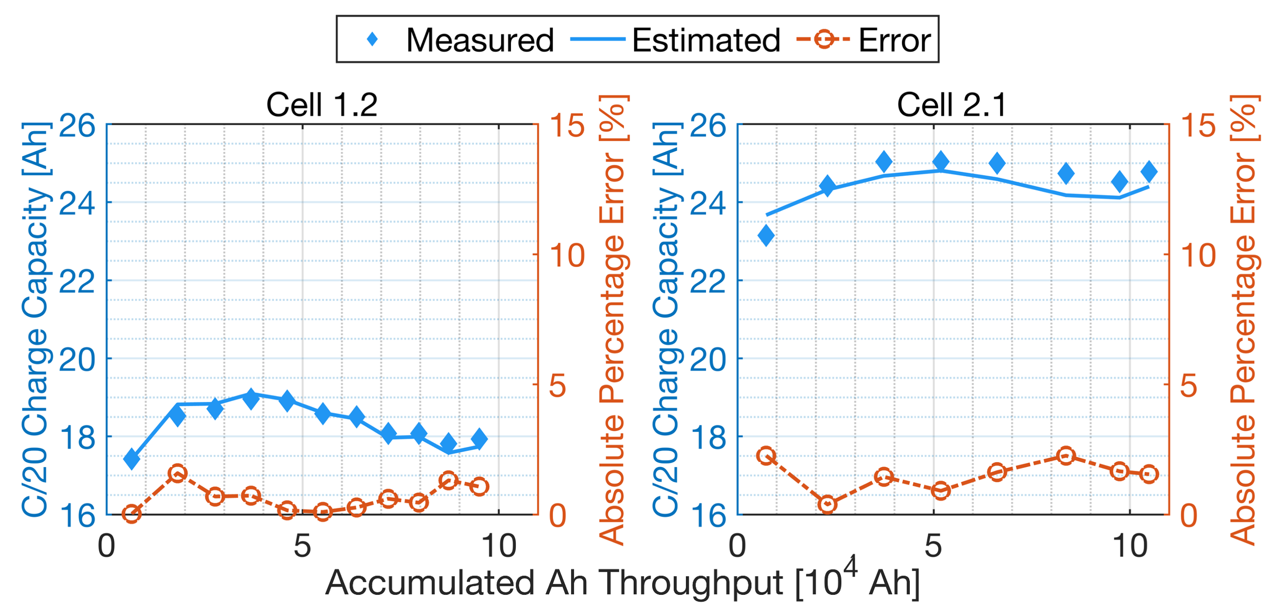
(a)

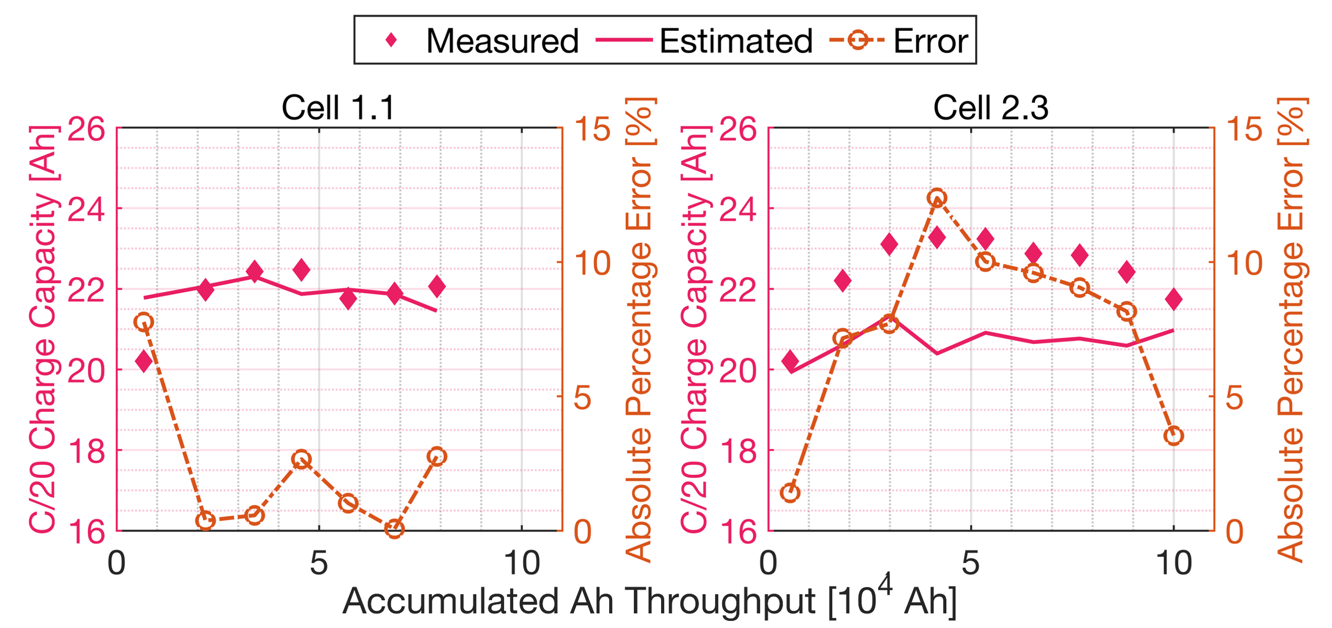
(b)

Figure 6: Offline ENR estimation results. (a) Estimation results for best performing test set (1.2, 2.1) which shows a good fit compared to the measured data with an absolute error percentage of less than or equal to 2% for all points. (b) Worst case estimation results for the test set (1.1, 2.3) as a result of inconsistent behavior in the input features of Cell 2.3 since it has a much larger error as compared to Cell 1.1 evident from the large percentage error of Cell 2.3.

V Adaptive Estimator

The health estimation of BMS₂ not only needs to be online but also adaptive, meaning that the estimator model should adapt as more online measurements are accumulated.

The aging-cycle charge throughput $Q_{age}$ is calculated as

$$Q_{age}(n)=\int_{t^{age}_{ch}(n)}^{t^{age}_{dis}(n)}I(t)\,dt,$$ (6)

where $Q_{age}(n)$, $t_{ch}^{age}(n)$, $t_{dis}^{age}(n)$, and $I(t)$ are shown in Fig. 5. The C/20 charge capacity $Q_{ch,C/20}$ is calculated as

$$Q_{ch,C/20}(n)=\int_{t^{C/20}_{ch}(n)}^{t^{C/20}_{dis}(n)}I(t)\,dt,$$ (7)

where $Q_{ch,C/20}(n)$, $t^{C/20}_{ch}(n)$, $t^{C/20}_{dis}(n)$, and $I(t)$ are shown in Fig. 5. The accumulated Ah throughput for the $n^{\text{th}}$ aging cycle $Ah_{n}^{age}$ is calculated as

$$Ah_{n}^{age}=\int_{0}^{t_{ch}^{age}}\Big{|}I(t)\Big{|}\,dt.$$ (8)

The accumulated Ah throughput for the $n^{\text{th}}$ C/20 charge-discharge cycle $Ah_{n}^{ch,C/20}$ is calculated as

$$Ah_{n}^{ch,C/20}=\int_{0}^{t_{ch}^{C/20}}\Big{|}I(t)\Big{|}\,dt.$$ (9)

Definition 1.

Given the monotonically increasing accumulated Ah-throughput sequence $\{Ah^{age}_{n}\}=\left(Ah^{age}_{1},Ah^{age}_{2},\cdots,Ah^{age}_{N}\right)$, $Ah^{age}_{i}\in\mathbb{R^{+}}$ and the aging-cycle charge throughput sequence $\{Q_{age}\}=\left(Q_{age}(1),Q_{age}(2),\cdots,Q_{age}(N)\right)$, $Q_{age}(n)\in\mathbb{R}^{+}$, then the aging-cycle charge throughput trajectory is a curve denoted by $Q_{age}(\{Ah^{age}_{n}\})$ or simply $Q_{age}$.

Definition 2.

Given the monotonically increasing accumulated Ah-throughput sequence $\{Ah_{n}\}=\left(0,Ah^{ch,c/20}_{2},\cdots,Ah^{ch,c/20}_{N}\right)$, $Ah^{ch,c/20}_{i}\in\mathbb{R^{+}}$ and the C/20 charge capacity sequence $\{Q_{ch,C/20}\}=\left(Q_{ch,C/20}(1),Q_{ch,C/20}(2),\cdots,Q_{ch,C/20}(N)\right)$, $Q_{ch,C/20}(n)\in\mathbb{R}^{+}$, the C/20 charge capacity trajectory is a curve denoted by $Q_{ch,C/20}(\{Ah^{ch,c/20}_{n}\})$ or simply $Q_{ch,C/20}$.

Remark: $Q_{ch,C/20}$ is calculated as shown in Fig. 5. For ease of notation, in the following derivations, the C/20 charge capacity sequence is simply denoted by $\{Q_{n}\}$ and $Q_{ch,C/20}$ is simply denoted by $Q$.

The normalized SOH indicator is the normalized C/20 charge capacity, calculated by

$$\bar{Q}(Ah_{n})=\frac{Q(Ah_{n})}{Q(0)},$$ (10)

where $Q(0)$ is the $C/20$ charge capacity of the cell measured at the beginning of the second life. For ease of notation, in the following derivations of this section, $Q(0)$ is simply denoted by $Q_{0}$.

Definition 3.

The $K$ cells in the training set are denoted by indices $1,\cdots,K$. Therefore, the C/20 charge capacity trajectories in the training set are $Q^{1},\cdots,Q^{K}$, denoted by $Q^{train}$. The aging cycle charge throughput trajectories in the training set are $Q^{1}_{age},\cdots,Q^{K}_{age}$, denoted by $Q^{train}_{age}$. Other than the aging cycle charge throughput trajectories, there are many other feature trajectories in the training set. We denote all feature trajectories in the training set by $X^{train}_{age}$.

Definition 4.

The one cell in the test set is denoted by index $z$. Therefore, the C/20 charge capacity trajectory in the test set is $Q^{z}$, denoted by $Q^{test}$. The aging cycle charge throughput trajectory in the test set is $Q^{z}_{age}$, denoted by $Q^{test}_{age}$. Other than the aging cycle charge throughput trajectories, there are many other feature trajectories in the test set. We denote all feature trajectories in the test set by $X^{test}_{age}$.

Remark: In this dataset, Cells 1.1, 1.2, 1.3, 2.1, 2.2, 2.3, 2.4 correspond to $k$ = 1, 2, 3, 4, 5, 6, 7, respectively. Cell 1.4 used for testing corresponds to $z$.

Definition 5.

The data-driven battery health estimator $\mathcal{E}_{H}$ is a type of data-driven estimator of the form:

$$\hat{Q}^{test} =f\left(X^{test}_{age},X^{train}_{age},Q^{train}\right),$$ (11)

where $f$ is a generic mapping function, $\hat{Q}^{test}$ represents the estimated C/20 charge capacity of the cell in the test set; $Q^{train}$ and $X^{train}_{age}$ can be found in Definition 3; $X^{test}_{age}$ can be found in Definition 4.

The estimation error $e_{n}$ is evaluated as

$$e =\hat{Q}^{test}-Q^{test},$$ (12)

where $Q^{test}$ can be found in Definition 4.

Stability is of practical importance for adaptive estimation laws as it ensures that the proposed estimation process does not result in divergence. This paper uses the notion of bounded-input, bounded-output (BIBO) stability as follows:

Definition 6.

A data-driven adaptive estimator $\mathcal{E}_{H}$ defined in Definition 5 is BIBO stable if for any bounded input signal with $\|X^{train}_{age}\|<\infty$, $\|X^{test}_{age}\|<\infty$, $\|Q^{train}\|<\infty$, $\|Q^{test}\|<\infty$, the error $e_{n}$ satisfies $\|e_{n}\|<\infty$.

V-A Clustering-based adaptive estimation

The clustering-based adaptive estimation algorithm aims to find the trajectory in the training set that is closest to the trajectory in the test set. The closeness metric is defined by the following distance function:

Definition 7.

The distance between two aging-cycle charge throughput trajectories $Q^{x}_{age}$ and $Q^{y}_{age}$ are

$$\text{dist}(Q^{x}_{age},Q^{y}_{age})=\sqrt{\sum_{i=1}^{n}\left(Q^{x}_{age}(Ah_{i})-Q^{y}_{age}(Ah_{i})\right)^{2}},$$

$$1\leq n\leq N.$$ (13)

Algorithm 1 Calculate Distance

function CalculateDistance($Q^{x}_{\text{age}}\left(Ah_{1},\cdots,Ah_{N}\right)$, $Q^{y}_{\text{age}}\left(Ah_{1},\cdots,Ah_{N}\right)$)

     $\text{distance}\leftarrow 0$ $\triangleright$ Initialize distance to zero

     for $i$ from $1$ to $n$ do

         $\text{diff}\leftarrow Q^{x}_{\text{age}}(Ah_{i})-Q^{y}_{\text{age}}(Ah_{i})$

         $\text{distance}\leftarrow\text{distance}+\text{diff}^{2}$

     end for

     $\text{distance}\leftarrow\sqrt{\text{distance}}$ $\triangleright$ Calculate the square root

     return distance $\triangleright$ Return the distance

end function

Remark: The pseudo-code to calculate the distance can be found in Algorithm 1. $\text{dist}(Q^{x}_{age},Q^{y}_{age})$ is non-negative and symmetric because of the properties of $\mathcal{L}^{2}$ norm. Compared to the nearest neighbor distance metric based on the latest measurements, this trajectory distance metric memorizes all historical differences between $Q^{x}_{age}$ and $Q^{y}_{age}$ and evaluates similarities based not only on instantaneous measurements but also on historical capacity measurements. Therefore, it is more robust in the presence of one-shot measurement noise. One shortcoming of this distance metric is that it requires more than one data point to make a definitive classification. However, in the long run, when the online BMS₂ has accumulated enough information, this additional data requirement can be easily met. This distance function can be easily generalized to measure the distance between other trajectories such as the C/20 charge capacity trajectory, etc.

Whenever a new sample of cell $z$ is collected, the classification is updated, giving the clustering index that cell $z$ is assumed to belong to:

Definition 8.

Classification index sequence for cell $z$ $\{S^{z}_{n}\}=\left(S^{z}_{1},S^{z}_{2},\cdots,S^{z}_{N}\right)$ is a discrete-time sequence defined by:

$$S^{z}_{n}= \underset{1\leq k\leq K}{\text{argmin}}\,\text{dist}\left(Q^{z}_{age}(\{Ah_{i}\}_{i\leq n}),Q^{k}_{age}(\{Ah_{i}\}_{i\leq n})\right),$$ (14)

where $Q^{z}_{age}$ and $Q^{k}_{age}$ are the aging-cycle charge trajectories of cell $z$ and $k$, respectively. The distance function $dist$ has been defined in Definition 7. An example of the cell classification is shown in Fig. 7. The pseudo-code to calculate the classification index sequence can be found in Algorithm 2.

Algorithm 2 Classification Index Sequence

function ClassificationIndexSequence($Q^{z}_{\text{age}}\left(Ah_{1},\cdots,Ah_{N}\right)$, $Q^{1}_{\text{age}}\left(Ah_{1},\cdots,Ah_{N}\right)$, $\cdots$, $Q^{K}_{\text{age}}\left(Ah_{1},\cdots,Ah_{N}\right)$)

     Initialize an empty sequence $S^{z}$

     for $n$ from $1$ to $N$ do

         $\text{minDist}\leftarrow\infty$ $\triangleright$ Initialize minimum distance to positive infinity

         $S_{n}^{z}\leftarrow 0$ $\triangleright$ Initialize the classification index for the current time step

         for $k$ from $1$ to $K$ do

              $\text{dist}\leftarrow$ CalculateDistance($Q^{z}_{\text{age}}\left(Ah_{1},Ah_{2},\cdots,Ah_{n}\right),Q^{k}_{\text{age}}\left(Ah_{1},Ah_{2},\cdots,Ah_{n}\right)$)

              if $\text{dist}<\text{minDist}$ then

                  $\text{minDist}\leftarrow\text{dist}$ $\triangleright$ Update minimum distance

                  $S_{n}^{z}\leftarrow k$ $\triangleright$ Update the classification index

              end if

         end for

         Append $S_{n}^{z}$ to $S^{z}$ $\triangleright$ Add the classification index to the sequence

     end for

     return $S^{z}$ $\triangleright$ Return the classification index sequence

end function

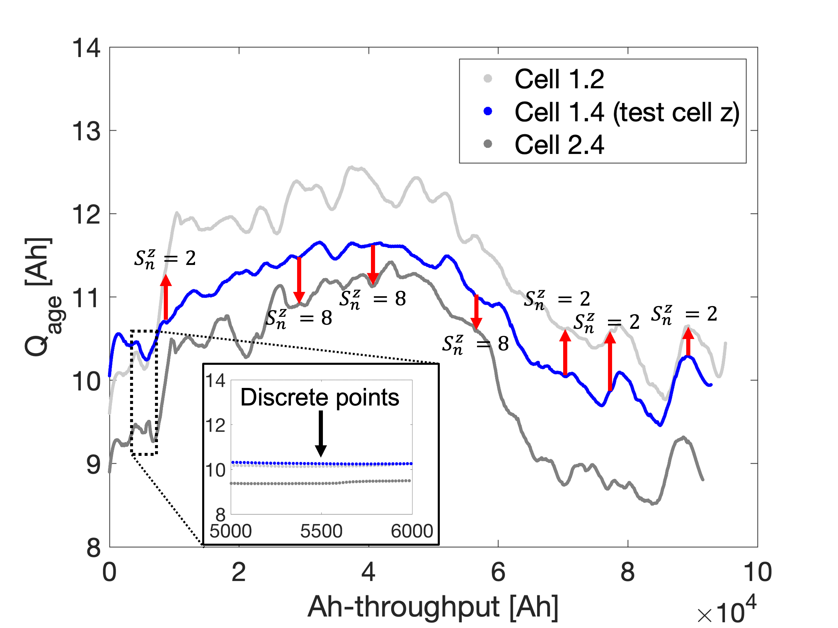
Figure 7: Example of cell classification defined in Definition 8 with Cell 1.4 as the test cell compared against Cell 1.2 ($S_{n}^{z}=2$) and Cell 2.4 ($S_{n}^{z}=8$). Red arrows points to the aging cycle charge trajectory with the minimum distance from $Q_{age}^{z}$ – where $z=1.4$ – at different Ah-throughputs. Zoomed plot shows that these are highly dense discrete points since $Q_{age}^{z}$ is extracted from every cycle.

Theorem 1.

Consider a data-driven estimator described in Definition 5. Let the battery cells 1 to cell $K$ be the training set and cell $z$ be the test set. If the model parameters are adapted, with the tunning parameters $\lambda_{k}$ according to

$$\lambda_{k}=\frac{\sum_{n=1}^{N}\leavevmode\resizebox{}{1.5pt}{$\chi$}(S^{z}_{n}=k)Ah_{n}}{\sum_{n=1}^{N}Ah_{n}},$$ (15)

where

$$\leavevmode\resizebox{}{1.5pt}{$\chi$}(S^{z}_{n}=k)=\begin{cases}1&\text{if}\,\,S^{z}_{n}=k,1\leq k\leq K\\ 0&\text{otherwise},\end{cases}$$ (16)

$I^{z}_{n}$ is defined in (14). Then the adaptive estimator, formulated as

$$\hat{Q}^{z}(Ah_{n}) =Q^{z}_{0}\hat{\bar{Q}}^{z}(Ah_{n}),$$ (17)

$$\hat{\bar{Q}}^{z}(Ah_{n}) =\sum_{k=1}^{K}\lambda_{k}\bar{Q}^{k}(Ah_{n}),$$ (18)

where $\hat{Q}^{z}$, the estimation target, represents the C/20 charge capacity of cell $z$, is BIBO stable.

Remark: The pseudo-code for the clustering-based adaptive estimation can be found in Algorithm 3. The tuning parameters $\lambda_{k}$ can be thought of as forgetting factors, assigning greater weight to the most recent classification result while retaining the memory of past classification outcomes to enhance robustness.

Algorithm 3 Clustering-Based Adaptive Estimator

$N$: Trajectory length or the number of data points on a trajectory

$K$: Number of cells in the training set

$S^{z}_{n}$: Array representing the classification index sequence

$Ah_{n}$: Array representing the accumulated $Ah$ throughput

$Q^{z}_{0}$: Initial SOH of cell $z$

Initialize an array for lambda values with size $K$: $\lambda=[0]*K$

Initialize an array for $\bar{Q}^{z}$ values with size $N$: $\bar{Q}^{z}=[0]*N$

Calculate the denominator for lambda:

$\text{denominator}=0$

for $n=1$ to $N$ do

     $\text{denominator}+=Ah_{n}[n]$

end for

Calculate lambda values for each training cell:

for $k=1$ to $K$ do

     $\text{numerator}=0$

     for $n=1$ to $N$ do

         if $S^{z}_{n}[n]=k$ then

              $\text{numerator}+=Ah_{n}[n]$

         end if

     end for

     $\lambda[k]$ = numerator/denominator

end for

Calculate $\bar{Q}^{z}$ for the cell in the test set:

for $n=1$ to $N$ do

     $\bar{Q}^{z}[n]=0$

     for $k=1$ to $K$ do

         $\bar{Q}^{z}[n]+=\lambda[k]\cdot\bar{Q}^{k}(Ah_{n}[n])$

     end for

end for

Calculate $Q^{z}$:

for $n=1$ to $N$ do

     $Q^{z}[n]=Q^{z}_{0}\cdot\bar{Q}^{z}[n]$

end for

The estimated SOH of the cell in test set is stored in the array $Q^{z}$

Proof.

From (15), $\lambda_{k}$ is designed to be positive. Moreover, $\lambda_{k}$ satisfies:

$$\sum_{k=1}^{K}\lambda_{k}=1,$$ (19)

This can be proved by:

$$\sum_{k=1}^{K}\lambda_{k} =\sum_{k=1}^{K}\frac{\sum_{n=1}^{N}\leavevmode\resizebox{}{1.5pt}{$\chi$}(S^{z}_{n}=k)Ah_{n}}{\sum_{n=1}^{N}Ah_{n}}$$ (20)

$$=\sum_{n=1}^{N}\frac{\sum_{k=1}^{K}\leavevmode\resizebox{}{1.5pt}{$\chi$}(S^{z}_{n}=k)Ah_{n}}{\sum_{n=1}^{N}Ah_{n}}$$ (21)

$$=\sum_{n=1}^{N}\frac{Ah_{n}}{\sum_{n=1}^{N}Ah_{n}}=1.$$ (22)

To prove the BIBO stability, from Definition 6, the $K$ SOH trajectories $\{Q_{n}^{1}\},\cdots,\{Q_{n}^{K}\}$ in the training set are bounded:

$$\|Q^{k}\|<\infty,\quad\quad\text{for}\;\;1\leq k\leq K.$$ (23)

From Definition 6, the SOH trajectory $\{Q^{z}_{n}\}$ in the test set is bounded:

$$\|Q^{z}\|<\infty.$$ (24)

The error trajectory between the estimated capacity and the true capacity follows:

$$\big{\|}\hat{Q}^{z}-Q^{z}\big{\|}\stackrel{{\scriptstyle(\ref{eqn:norm_q_z})}}{{=}} \Bigg{\|}Q_{0}^{z}\hat{\bar{Q}}^{z}-Q^{z}\Bigg{\|}$$ (25)

$$\stackrel{{\scriptstyle(\ref{eqn:norm_q_z_decomp})}}{{=}} \Bigg{\|}Q_{0}^{z}\sum_{k=1}^{K}\lambda_{k}\bar{Q}^{k}-Q^{z}\Bigg{\|}$$ (26)

$$\stackrel{{\scriptstyle(\ref{eqn:lambda_sum_property})}}{{=}} \Bigg{\|}Q_{0}^{z}\sum_{k=1}^{K}\lambda_{k}\bar{Q}^{k}-\sum_{k=1}^{K}\lambda_{k}Q^{z}\Bigg{\|}$$ (27)

$$\stackrel{{\scriptstyle(\ref{eqn:norm_q_ch})}}{{=}} \Bigg{\|}Q_{0}^{z}\sum_{k=1}^{K}\lambda_{k}\bar{Q}^{k}-Q_{0}^{z}\sum_{k=1}^{K}\lambda_{k}\bar{Q^{z}}\Bigg{\|}$$ (28)

$$= Q_{0}^{z}\Bigg{\|}\sum_{k=1}^{K}\lambda_{k}\left(\bar{Q}^{k}-\bar{Q}^{z}\right)\Bigg{\|}.$$ (29)

From (19) and (29)

$$\big{\|}\hat{Q}^{z}-Q^{z}\big{\|}\leq Q_{0}^{z}\underset{1\leq k\leq K}{\text{max}}\{\big{\|}\bar{Q}^{k}-\bar{Q}^{z}\big{\|}\}$$ (30)

$$\leq \underset{1\leq k\leq K}{\text{max}}\{\big{\|}Q^{k}\big{\|}\}+\|Q^{z}\|<\infty.$$ (31)

Therefore, the error trajectory is bounded. From Definition 6, the BIBO stability is guaranteed. ∎

This proof aims to demonstrate that the estimation error of the test cell’s SOH is bounded by a function of the SOH values of all the cells in the training set.

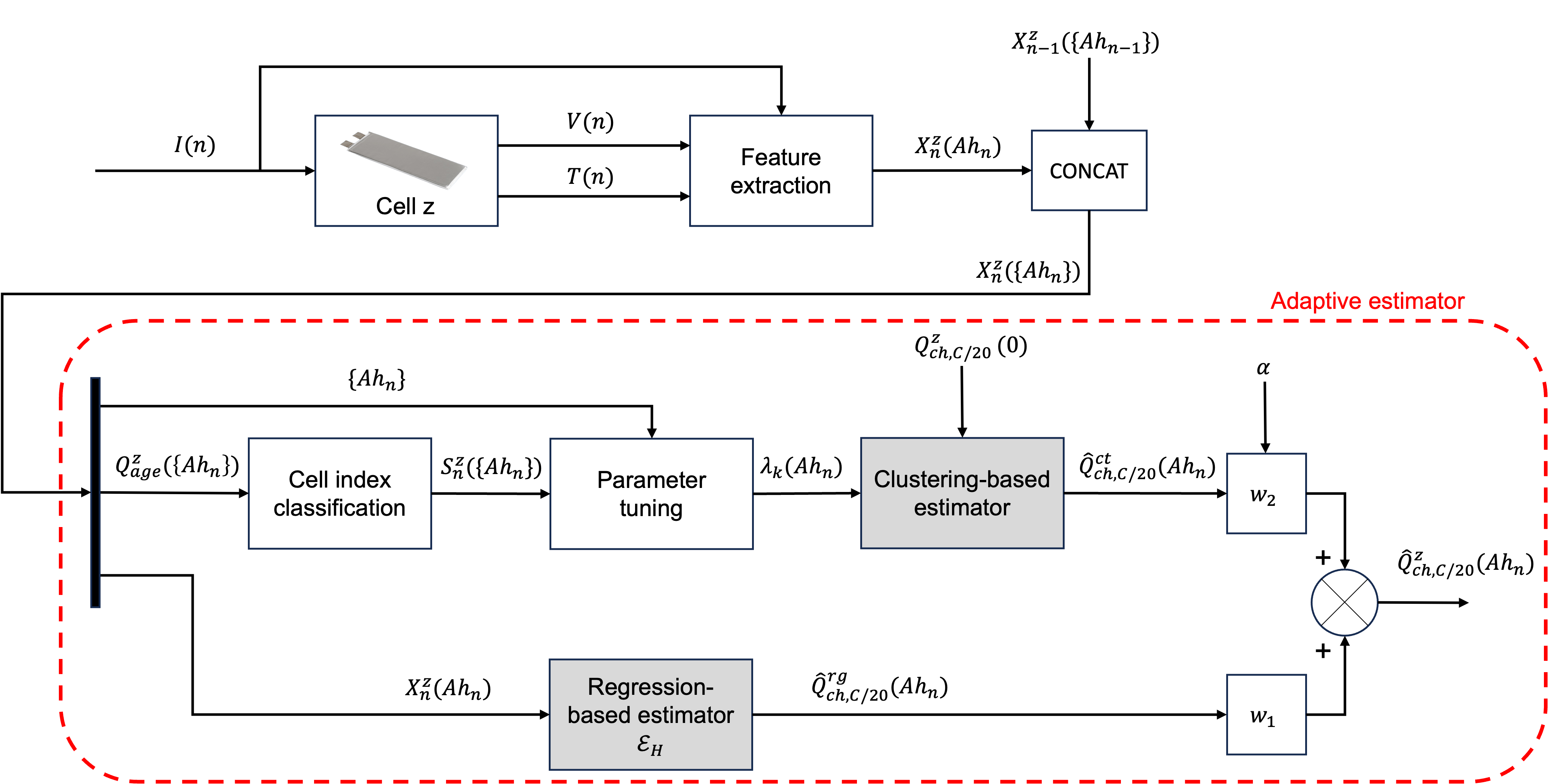
Figure 8: Block structure showing current $I(n)$, voltage $V(n)$, and cell surface temperature $T(n)$ used to extract features at time $n$. The extracted features are concatenated with features at time instant $n-1$ and this complete sequence of features is input to the adaptive estimator. Output $\hat{Q}_{ch,C/20}^{z}$ is obtained through a weighted sum of the output from clustering-based estimator and regression-based estimator (offline ENR model). Clustering-based estimator uses only the complete sequence of Ah-throughput $\{Ah_{n}\}$ and aging cycle charge trajectory $Q^{z}_{age}(\{Ah_{n}\})$ that is observed while all the signals from $X_{n}^{z}$ at the current time instance are used for the regression-based estimation.

V-B Adaptive Estimation by Combining the Clustering and Regression

The clustering-based method proposed in this study can exhibit a significant classification error when there is limited observation available for the cell under test. To address this limitation, we combinine the clustering-based estimation and the regression-based estimation.

Theorem 2.

Consider a data-driven estimator described in Definition 5. The adaptive weight parameters $w_{1},w_{2}\in\mathbb{R^{+}}$ follows

$$w_{2} =\begin{cases}\alpha Ah&\text{if }\alpha Ah<0.5\\ 0.5&\text{otherwise}\end{cases}$$ (32)

$$w_{1} =1-w_{2},$$ (33)

where $\alpha$ is a fixed constant. Then the adaptive estimator, formulated as

$$\hat{Q}^{z}(Ah_{n})=w_{1}\hat{Q}^{rg}(Ah_{n})+w_{2}\hat{Q}^{ct}(Ah_{n}),$$ (34)

is BIBO stable.

Remark 1: The adaptive estimation is obtained by summing the two estimation results with weights assigned to them. The weight parameters $w_{1}$ and $w_{2}$ allocate increasing importance to the online model as time progresses, while still preserving the influence of the offline model.

Remark 2: $\alpha$ can be interpreted as a learning-rate constant, measured in units of $Ah^{-1}$, with a range of values from $0$ to $+\infty$. It is recommended to initially set $\alpha$ to $\alpha=1/20Ah_{\text{max}}$ at the outset, where $Ah_{\text{max}}$ represents the largest Ah throughput that the batteries are expected to be cycled during its second life. Subsequently, $\alpha$ can be adjusted using the data in the training set. For example, the designer can gradually increase $\alpha$ until the point at which the validation error begins to rise. Sensitivity analysis of $\alpha$ for Cell 1.2, 1.4, and 2.3 is shown in Section V-B1.

Proof.

The error trajectory between the estimated capacity and the true capacity follows:

$$\|\hat{Q}^{z}-{Q}^{z}\|$$ (35)

$$\stackrel{{\scriptstyle(\ref{eqn:merge_est})}}{{=}} \Bigg{\|}\left(w_{1}\hat{Q}^{rg}+w_{2}\hat{Q}^{rg}\right)-(w_{1}+w_{2}){Q}^{z})\Bigg{\|}$$ (36)

$$= \big{\|}w_{1}(\hat{Q}^{rg}-{Q}^{z})+w_{2}(\hat{Q}^{ct}-{Q}^{z})\big{\|}$$ (37)

$$\leq w_{1}\big{\|}\hat{Q}^{rg}-Q^{z}\big{\|}+w_{2}\big{\|}\hat{Q}^{ct}-Q^{z}\big{\|}$$ (38)

From Theorem 1, the second term $w_{2}\|\hat{Q}^{ct}-Q^{z}\|$ in (38) is bounded. To prove the stability, from Definition 6, the feature trajectories in the training set are bounded:

$$\|X^{train}_{age}\|<\infty.$$ (39)

From (39) and (24), the first term in (38) is bounded by

$$\big{\|}\hat{Q}^{rg}-Q^{z}\big{\|}$$ (40)

$$= \big{\|}X^{train}_{age}\beta+\beta_{0}-Q^{z}\big{\|}$$ (41)

$$\leq \|X^{train}_{age}\|\|\beta\|+\|\beta_{0}\|+\|Q^{z}\|<\infty.$$ (42)

Therefore, the error trajectory is bounded and the BIBO stability is guaranteed. ∎

The complete flow of information for the adaptive estimator is shown in Fig. 8. In summary, the adaptive law used in the estimation process does not cause the estimation to diverge, and the worst-case error in health estimation can be bounded. The size of the error ball is determined by the errors of the offline model and adaptive model. Furthermore, the radius of the error ball can be further reduced by tunning the gains $w$ and $\lambda$.

V-B1 Sensitivity analysis of learning-rate constant $\alpha$

For the adaptive estimator given in Section V-B, $\alpha$ is used to adapt $w_{2}$ to control the contribution of $\hat{Q}^{ct}(Ah_{n})$ in the output. The range is given by $\alpha=[0,+\infty)$, which means it is important to choose a suitable value of $\alpha$ to ensure the best performance from the estimator. In this sensitivity analysis, three different ranges of $\alpha$ values are tested, and each range consists of five linearly spaced points, including the boundary values. These ranges are given by: 1) Range $r_{1}=[0,5\times 10^{-6}]$, 2) Range $r_{2}=[6\times 10^{-6},1]$, and 3) Range $r_{3}=[11,100]$ as shown in Fig. 9.

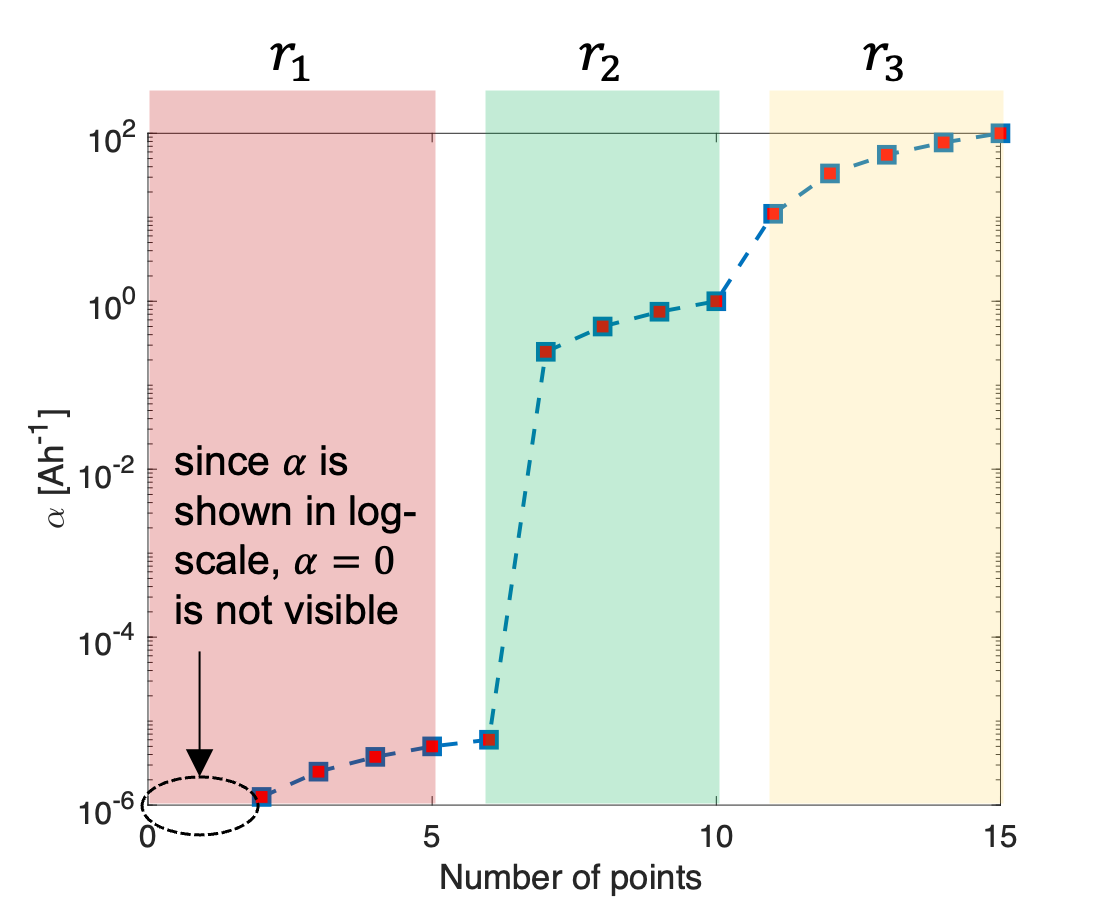
Figure 9: Range of $\alpha$ values used for sensitivity analysis shown on log-scale.

For sensitivity analysis, the RMSE error is observed for different $\alpha$ values and the results are compared to the current $\alpha$ value used in our results. Fig. 10 shows the sensitivity of $\alpha$ for cell 1.2. It can be seen that $\alpha_{current}$ – the current value of $\alpha$ – gives the lowest RMSE for the entire range of values. In fact, using values smaller or greater than $\alpha_{current}$ increases the RMSE value. Repeating the same analysis for cell 1.4 as shown in Fig. 11, we can see that $\alpha_{current}$ does not give the smallest RMSE; instead, the smallest RMSE is obtained at $\alpha=6\times 10^{-6}$. An extra set of linearly spaced 10 points between $[6\times 10^{-6},0.25]$ is analyzed and it can be seen that lowest RMSE is still obtained at the same value. It should be noted that $\alpha=5\times 10^{-6}$ is a close second in terms of lowest RMSE with a difference of less than $0.1\%$ for the lowest RMSE value.

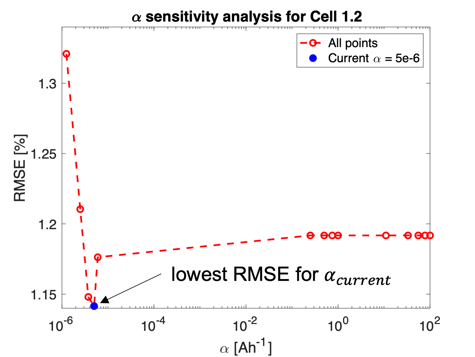
Figure 10: Sensitivity analysis of $\alpha$ for Cell 1.2 with $\alpha_{current}$ giving the lowest RMSE value

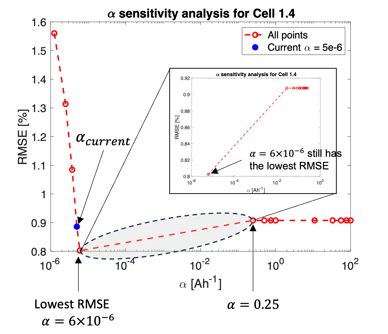
Figure 11: Sensitivity analysis of $\alpha$ for Cell 1.4 with $\alpha=6\times 10^{-6}>\alpha_{current}$ giving the lowest RMSE value

Finally, for Cell 2.3, the sensitivity analysis results are shown in Fig. 12. It can be seen that neither $\alpha=5\times 10^{-6}$ or $\alpha=6\times 10^{-6}$ give the lowest RMSE value. Instead, by analyzing 18 further points between $[6\times 10^{-6},0.25]$, it can be seen that the lowest RMSE is obtained for a range of values of $\alpha\geq 2.8\times 10^{-4}$. One thing to note here is that Cell 2.3 has the largest errors in the offline ENR model which means relativity larger contribution of the clustering-based estimator $\hat{Q}^{ct}(Ah_{n})$ is needed to improve the estimation of the model.

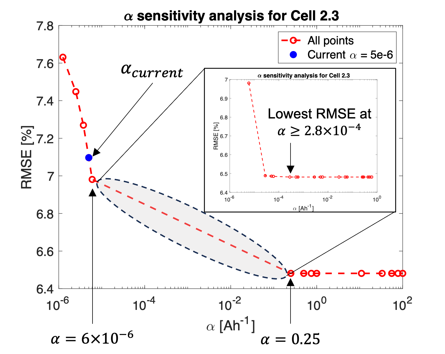
Figure 12: Sensitivity analysis of $\alpha$ for Cell 2.3 with $\alpha\geq 2.8\times 10^{-4}>\alpha_{current}$ giving the lowest RMSE values

VI Results and Discussion

The performance of the proposed online adaptive estimation algorithm is demonstrated in several case studies. In the first demonstration, we leave out Cell 1.4 for testing while training the model using the remaining seven cells. The C/20 charge capacity trajectories estimated by the ENR model, online adaptive model, and measured capacity are illustrated in Figs. 13(a), (b), and (c), respectively.

Initially, when the Ah throughput is lower, the weight $w_{1}$ is large, while the weight $w_{2}$ is small. The ENR-based estimate dominates the overall estimate. Therefore, the ENR model and adaptive model coincide at the same starting point, as demonstrated in Fig. 13(a). As Ah throughput increases to $Ah>2\times 10^{4}$ Ah, the classification index converges to the right cluster (cluster 8 / Cell 2.4), as depicted in Fig. 13(c). However, it is observed that after Ah throughput increases to $Ah>6.5\times 10^{4}$ Ah, the classification index is again perturbed to the wrong cluster (cluster 2 / Cell 1.2). Due to the weight adaptation law (15), the overall estimation output is only slightly impacted by the wrong classification.

Because the adaptive SOH estimator continuously processes the real-time influx of data, it yields reduced estimation errors. As displayed in Fig. 13(b), employing solely the ENR model yields a maximum absolute pointwise percentage error of 3 %, and a root mean squared pointwise percentage error of 1.8166 %. In contrast, by leveraging the online adaptive model that combines the ENR-based estimation and clustering-based estimation, the maximum pointwise percentage error decreases to 2 %, and the root mean squared pointwise percentage error decreases to 0.8610 %.

This example demonstrates the impacts of weight adaptation. Weight $w$ balances the contributions of the offline ENR model and the online clustering-based model. It avoids the important hazards that the online clustering-based model causes by under-informed classification in the beginning when little data is collected. Weight $\lambda$ balances the contributions of the current-step classification result and historical-steps classification results. These historical-steps classification results are memorized by summing their corresponding Ah throughput. This effectively decreases the high sensitivity of the online clustering-based estimation method to the current-step classification result.

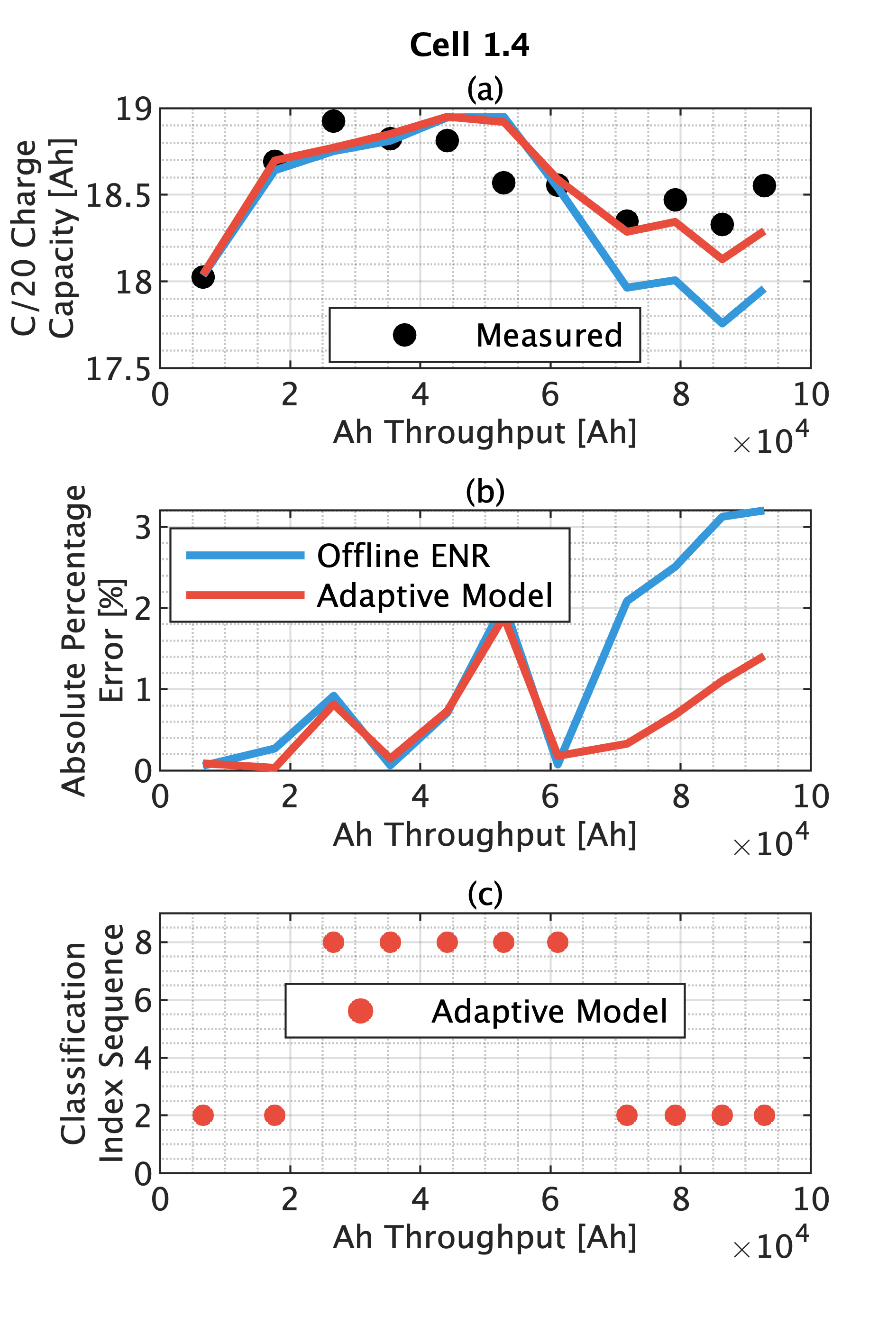
Figure 13: Performance evaluation of the online adaptive estimator for cell 1.4. (a) The C/20 charge capacity trajectories estimated from the offline Elastic-Net Regression (ENR) and online adaptive model are compared against the measured capacity. (b) The pointwise absolute capacity estimation percentage error of the offline ENR is compared against that of the online adaptive model. The Root Mean Square Error (RMSE) of the online adaptive model is 0.8610 %. (c) The classification index sequence, as defined in Definition 8, of the online adaptive estimator.

In the second demonstration shown in Fig. 14, the online adaptive estimation algorithm is tested on cell 2.3, in which the ENR has illustrated a poor performance. The clustering-based estimator starts to behave stable after Ah throughput $Ah>2\times 10^{4}\text{Ah}$. The classification results converge toward the cluster 1 (centered at cell 1.1), as depicted in Fig. 14(c). As the clustering model becomes more reliable, placing more weight on the clustering-based estimation enhances the overall estimation performance. The pointwise percentage RMSE improves to 7.2708 %, compared to the 7.8190 % by pure offline ENR method.

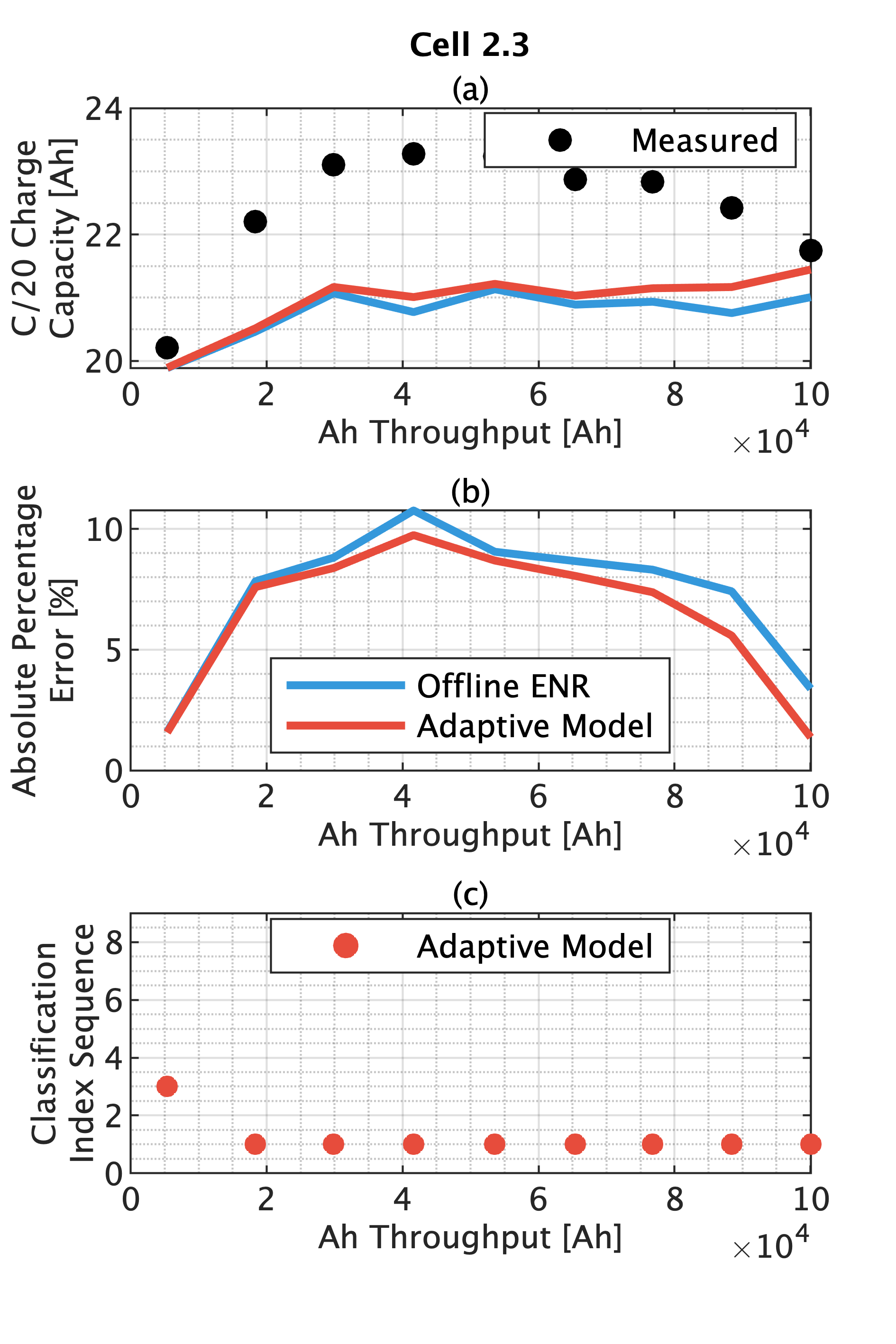
Figure 14: Performance evaluation of the online adaptive estimator for cell 1.4. (a) The C/20 charge capacity trajectories estimated from the offline Elastic-Net Regression (ENR) and online adaptive model are compared against the measured capacity. (b) The pointwise absolute capacity estimation percentage error of the offline ENR is compared against that of the online adaptive model. The Root Mean Square Error (RMSE) of the online adaptive model is 7.2708 %. (c) The classification index sequence, as defined in Definition 8, of the online adaptive estimator.

In the last demonstration shown in Fig. 15, the online adaptive estimation algorithm is tested on Cell 1.2, in which the ENR has already illustrated a good performance. As shown in Fig. 15, adding the online adaptive estimator can further reduce the pointwise percentage RMSE of capacity estimation from 1.4686 % to 1.2182 %.

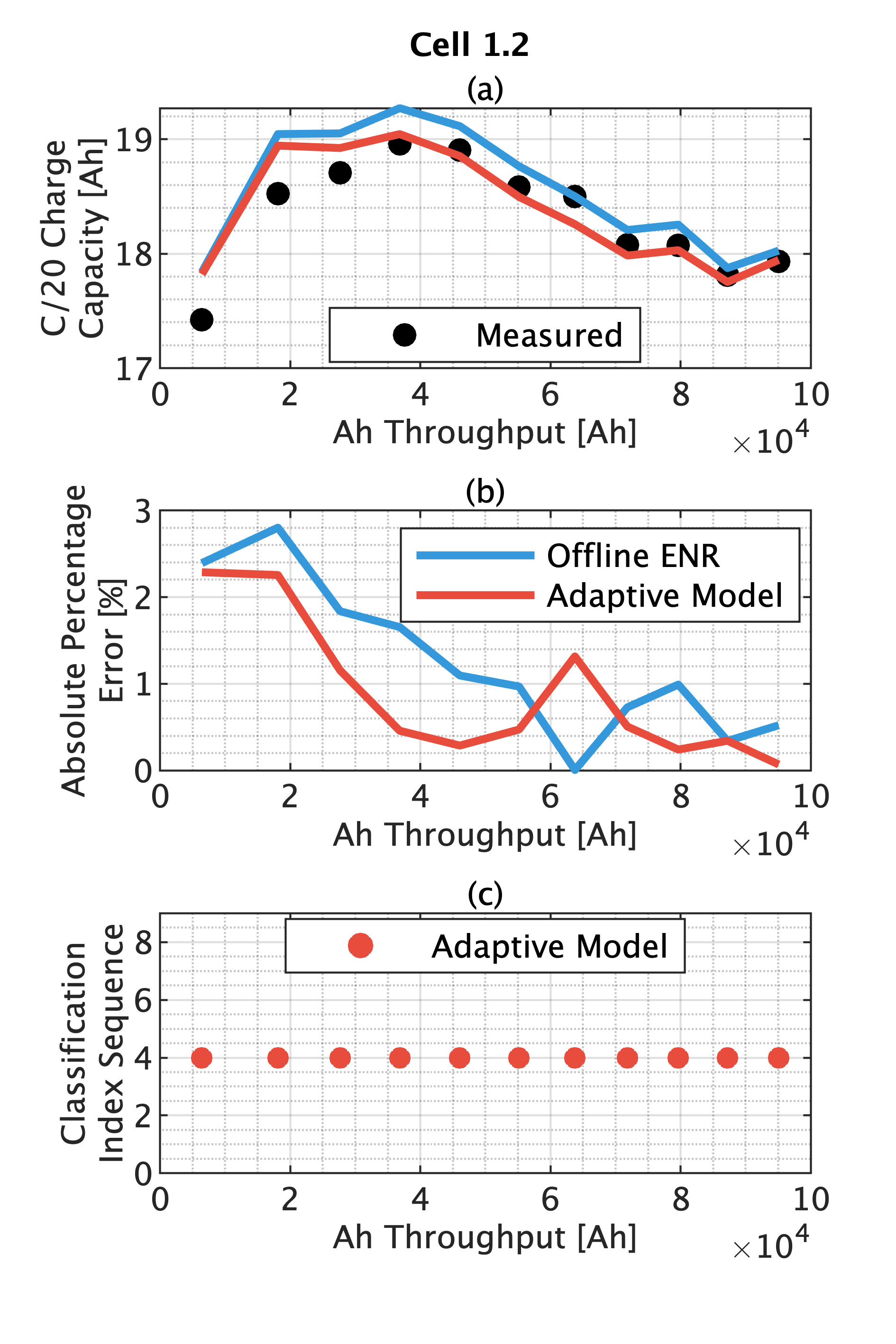
Figure 15: Performance evaluation of the online adaptive estimator for cell 1.4. (a) The C/20 charge capacity trajectories estimated from the offline Elastic-Net Regression (ENR) and online adaptive model are compared against the measured capacity. (b) The pointwise absolute capacity estimation percentage error of the offline ENR is compared against that of the online adaptive model. The Root Mean Square Error (RMSE) of the online adaptive model is 1.2182 %. (c) The classification index sequence, as defined in Definition 8, of the online adaptive estimator.

VII Conclusions

Due to its high flexibility and model agnosticism, data-driven health estimation has emerged as a valid and viable method for assessing the health of SL batteries. To enable the in-the-field operation of SL battery energy storage systems, we present an online adaptive health data-driven estimation method with guaranteed stability. The clustering-based estimation is combined together with the elastic-net regression. We have validated this method using a dataset of lab-aged second-life batteries retired from commercial EVs.

ACKNOWLEDGEMENTS

The authors would like to thank Surinder Singh and Ratnesh Sharma for collecting data described in [27] and StorageX Initiative within the Precourt Institute of Energy at the Stanford University for the financial support.

References

- [1] N. Lutsey, M. Grant, S. Wappelhorst, and H. Zhou, “Power play: How governments are spurring the electric vehicle industry.” ICCT Washington, DC, USA, 2018.
- [2] J. Eddy, A. Pfeiffer, and J. van de Staaij, “Recharging economies: The ev-battery manufacturing outlook for europe,” McKinsey & Company, 2019.
- [3] P. Pavlínek, “Transition of the automotive industry towards electric vehicle production in the east european integrated periphery,” Empirica, vol. 50, no. 1, pp. 35–73, 2023.
- [4] B. Jones, V. Nguyen-Tien, and R. J. Elliott, “The electric vehicle revolution: Critical material supply chains, trade and development,” The World Economy, vol. 46, no. 1, pp. 2–26, 2023.
- [5] Q. Dong, S. Liang, J. Li, H. C. Kim, W. Shen, and T. J. Wallington, “Cost, energy, and carbon footprint benefits of second-life electric vehicle battery use,” iScience, 2023.
- [6] J. Lu, R. Xiong, J. Tian, C. Wang, C.-W. Hsu, N.-T. Tsou, F. Sun, and J. Li, “Battery degradation prediction against uncertain future conditions with recurrent neural network enabled deep learning,” Energy Storage Materials, vol. 50, pp. 139–151, 2022.
- [7] A. Weng, E. Dufek, and A. Stefanopoulou, “Battery passports for promoting electric vehicle resale and repurposing,” Joule, pp. 837––842, 2023.
- [8] X. Hu, X. Deng, F. Wang, Z. Deng, X. Lin, R. Teodorescu, and M. G. Pecht, “A Review of Second-Life Lithium-Ion Batteries for Stationary Energy Storage Applications,” Proceedings of the IEEE, vol. 110, no. 6, pp. 735–753, jun 2022.
- [9] G. Pozzato, S. B. Lee, and S. Onori, “Modeling degradation of Lithium-ion batteries for second-life applications: preliminary results,” CCTA 2021 - 5th IEEE Conference on Control Technology and Applications, pp. 826–831, 2021.
- [10] Y. Jiang, J. Jiang, C. Zhang, W. Zhang, Y. Gao, and N. Li, “State of health estimation of second-life lifepo4 batteries for energy storage applications,” Journal of Cleaner Production, vol. 205, pp. 754–762, 2018. [Online]. Available: https://www.sciencedirect.com/science/article/pii/S0959652618328725
- [11] J. Wei, G. Dong, and Z. Chen, “Remaining useful life prediction and state of health diagnosis for lithium-ion batteries using particle filter and support vector regression,” IEEE Transactions on Industrial Electronics, vol. 65, no. 7, pp. 5634–5643, 2018.
- [12] A. Takahashi, A. Allam, and S. Onori, “Evaluating the feasibility of batteries for second-life applications using machine learning,” iScience, vol. 26, no. 4, p. 106547, 2023. [Online]. Available: https://doi.org/10.1016/j.isci.2023.106547
- [13] C. Zhang, J. Jiang, W. Zhang, Y. Wang, S. M. Sharkh, and R. Xiong, “A novel data-driven fast capacity estimation of spent electric vehicle lithium-ion batteries,” Energies, vol. 7, no. 12, pp. 8076–8094, 2014. [Online]. Available: https://www.mdpi.com/1996-1073/7/12/8076
- [14] A. Bhatt, W. Ongsakul, N. Madhu, and J. G. Singh, “Machine learning-based approach for useful capacity prediction of second-life batteries employing appropriate input selection,” International Journal of Energy Research, vol. 45, no. 15, pp. 21 023–21 049, dec 2021.
- [15] X. Li, Y. Dai, Y. Ge, J. Liu, Y. Shan, and L.-Y. Duan, “Uncertainty modeling for out-of-distribution generalization,” arXiv preprint arXiv:2202.03958, 2022.
- [16] Y. Zhang, T. Wik, J. Bergström, M. Pecht, and C. Zou, “A machine learning-based framework for online prediction of battery ageing trajectory and lifetime using histogram data,” Journal of Power Sources, vol. 526, p. 231110, 2022.
- [17] C. She, Y. Li, C. Zou, T. Wik, Z. Wang, and F. Sun, “Offline and online blended machine learning for lithium-ion battery health state estimation,” IEEE Transactions on Transportation Electrification, vol. 8, no. 2, pp. 1604–1618, 2021.
- [18] J. Zhou, D. Liu, Y. Peng, and X. Peng, “An optimized relevance vector machine with incremental learning strategy for lithium-ion battery remaining useful life estimation,” in 2013 IEEE International Instrumentation and Measurement Technology Conference (I2MTC). IEEE, 2013, pp. 561–565.
- [19] Y. Xing, E. W. Ma, K.-L. Tsui, and M. Pecht, “An ensemble model for predicting the remaining useful performance of lithium-ion batteries,” Microelectronics Reliability, vol. 53, no. 6, pp. 811–820, 2013. [Online]. Available: https://www.sciencedirect.com/science/article/pii/S0026271412005227
- [20] Y. Zhang, T. Wik, J. Bergström, M. Pecht, and C. Zou, “A machine learning-based framework for online prediction of battery ageing trajectory and lifetime using histogram data,” Journal of Power Sources, vol. 526, apr 2022.
- [21] K. Liu, Q. Peng, Y. Che, Y. Zheng, K. Li, R. Teodorescu, D. Widanage, and A. Barai, “Transfer learning for battery smarter state estimation and ageing prognostics: Recent progress, challenges, and prospects,” Advances in Applied Energy, p. 100117, 2022.
- [22] J. Lu, R. Xiong, J. Tian, C. Wang, and F. Sun, “Deep learning to estimate lithium-ion battery state of health without additional degradation experiments,” Nature Communications, vol. 14, no. 1, p. 2760, 2023.
- [23] F. Von Bülow and T. Meisen, “State of health forecasting of heterogeneous lithium-ion battery types and operation enabled by transfer learning,” in PHM Society European Conference, vol. 7, no. 1, 2022, pp. 490–508.
- [24] S. Zhang, H. Zhu, J. Wu, and Z. Chen, “Voltage relaxation-based state-of-health estimation of lithium-ion batteries using convolutional neural networks and transfer learning,” Journal of Energy Storage, vol. 73, p. 108579, 2023.
- [25] K. A. Severson, P. M. Attia, N. Jin, N. Perkins, B. Jiang, Z. Yang, M. H. Chen, M. Aykol, P. K. Herring, D. Fraggedakis et al., “Data-driven prediction of battery cycle life before capacity degradation,” Nature Energy, vol. 4, no. 5, pp. 383–391, 2019.
- [26] C. P. Aiken, E. R. Logan, A. Eldesoky, H. Hebecker, J. Oxner, J. Harlow, M. Metzger, and J. Dahn, “Li[\chNi_Mn_Co_] \ceO2 as a superior alternative to \ceLiFePO4 for long-lived low voltage li-ion cells,” Journal of The Electrochemical Society, vol. 169, no. 5, p. 050512, 2022.
- [27] X. Cui, M. A. Khan, G. Pozzato, R. Sharma, S. Singh, and S. Onori, “From exhausted to empowered: Experiments, data analysis, and health estimation for second-life batteries,” Cell Reports Physical Science (under review).
- [28] P. M. Attia, A. Bills, F. B. Planella, P. Dechent, G. Dos Reis, M. Dubarry, P. Gasper, R. Gilchrist, S. Greenbank, D. Howey et al., ““knees” in lithium-ion battery aging trajectories,” Journal of The Electrochemical Society, vol. 169, no. 6, p. 060517, 2022.