Analytical solutions for optimal photon absorption into inhomogeneous spin memories

Abstract

We investigate for optimal photon absorption a quantum electrodynamical model of an inhomogeneously-broadened spin ensemble coupled to a single-mode cavity. We consider a one-photon input pulse and obtain a simple one-parameter form for its optimal shape for absorption in the spin ensemble. Solutions to this problem are developed without using perturbation theory concerning the spin ensemble. Furthermore, we exploit the possibility of modulating the frequency and coupling rate of the resonator. We show some optimal scenarios and demonstrate the usefulness of our approach for the design of efficient quantum memories. In particular, we find the optimal cooperativity for different parameters and identify cases where absorption with a success probability larger than $99\%$ is achieved.

I Introduction

Information transport is fundamental to the scalability of both short and long-range quantum architectures. A chief candidate is the flying mode approach where information carriers are themselves quantum objects that must retain coherence over the intermediary channel. Applications of quantum transport range widely, including quantum communication Sangouard et al. (2011), remote sensing Schnabel et al. (2010), optical computation Kok et al. (2007); Slussarenko and Pryde (2019); Cohen and Mølmer (2018), error correction Kerckhoff et al. (2010); Martin et al. (2015), and cryptography Pirandola et al. (2020). For quantum computing purposes, flying modes are key to scalability, e.g. via traveling electrons Fujita et al. (2017); Li et al. (2018), ions Kaushal et al. (2020), atoms Bluvstein et al. (2022), or photons Roch et al. (2014); Reiserer et al. (2014); Brekenfeld et al. (2020) between static qubits. They enable larger spacings and better connectivity, and connection to storage qubits with longer lifetimes Grezes et al. (2014). In particular, we study here the situation where the quantum memory is composed of multiple inhomogeneously cavity-coupled and broadened matter qubits, as can be formed with spins Steger et al. (2012); Grezes et al. (2014); Ranjan et al. (2020); O’Sullivan et al. (2022), Rydberg atomsDistante et al. (2017); Motzoi and Mølmer (2018); Jiang et al. (2019), and ions Ortu et al. (2018). For this purpose, using ensembles of spins has several advantages, including greatly enhanced cavity-coupling and multi-mode random-access storage.

We examine the absorption of the flying photon by the spin ensemble. We analytically derive absorption equations and numerically optimize the external drive to minimize the time and maximize the efficiency. The efficient storage of a photon into a single atom has already been investigated both theoretically Trautmann and Alber (2016) and experimentally Brekenfeld et al. (2020). However, in the case of a spin ensemble, each spin is characterized by an individual dipole coupling and its Larmor frequency within an inhomogeneous line width. The mathematical description of a similar system was introduced almost three decades ago Garraway and Knight (1996); Garraway (1997), where the authors treated the spontaneous decay of an atomic system into a photonic band gap. Here, a single mode of the radiation field interacts with spins having Larmor frequencies in a band gap. This model is usually investigated under semi-classical approximations or by employing perturbation techniques Kurucz et al. (2011); Diniz et al. (2011); Julsgaard and Mølmer (2012); Afzelius et al. (2013); Julsgaard et al. (2013). These approaches focus on the Heisenberg picture, where expectation values of the system’s operators are calculated, and this leads to a system of infinitely many differential equations. Our focus lies on the Schrödinger picture, where the solution to the time evolution of the state becomes tractable due to the presence of a single excitation.

In this work, we have three aims: first, to present a minimal model with a spin ensemble and a cavity, which can describe the storage process of an incoming photon with tunable decay rate and detuning of the cavity; second, to non-perturbatively describe the time evolution of this model with arbitrary input waveforms and inhomogeneous broadening distributions, including Lorentzians and Gaussians; third, to probe the optimality of the storage with simple few-parameter pulses. In particular, we investigate both closed-form and numerically optimized solutions, both for sequential absorption of the photon into the cavity followed by the spin ensemble, or directly from the environment into the ensemble. Note that our method is general beyond quantum memories and largely applicable to the wide range of applications mentioned above.

The paper is organized as follows. In Sec. II, we set notation, introduce the Hamiltonian model describing the external modes of the radiation field, and derive the input-output theory for ensemble spins in Schrödinger picture. In Sec.  III, we derive the exact solution to the complete time evolution of the system. In Sec. IV, we analyze the two-step sequential excitation of the cavity and spin ensemble, which is made possible by the controllability of the cavity parameters, and find a globally optimal protocol. In Sec. V, we analyze a direct, single-step approach to the excitation of the spin ensemble. Further optimizations using both numerical and analytical approaches are presented. In Sec. VI, we summarize our conclusions. Details supporting the main text are collected in the Appendix.

II Input-output formalism in the Schrödinger picture

In this section, we develop the system model for the inhomogeneous spin-ensemble system coupled to a microwave cavity and fix the required notation. For this purpose, we review the input-output formalism, and in particular we re-derive it in the context of the Schrödinger picture, which is ideally suited to the situation of having a single photon in the input light field. This derivation can be contrasted with a similar input-output theory derivation in Motzoi and Mølmer (2018), where a homogeneous ensemble of Rydberg atoms is also considered in the Schrödinger picture.

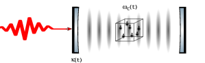
Let us consider a single cavity mode interacting with an external radiation field and an ensemble of $N$ spins as schematically depicted in Fig. 1. We assume that the dipole and rotating-wave approximations are valid for this setup. The $i$th spin system comprises a ground state level $|{0}\rangle_{i}$ and an excited level $|{1}\rangle_{i}$ of different parity and they are separated by an energy difference $\hbar\omega_{i}$. It is assumed that the frequency $\omega_{i}$ is inhomogeneously broadened around a central frequency $\omega_{s}$. The dipole coupling $g_{i}$ of each spin, which involves the transition dipole moment of the states and the normalized mode function of the single-mode radiation field in the cavity, is distributed also inhomogeneously. A microscopic model of the external radiation field allows us to describe the propagation of photons outside the cavity and photons can enter this cavity by transmission through a mirror. We also assume that the typical interaction times are small enough to neglect the spontaneous emission of photons from any excited state $|{1}\rangle_{i}$. Within these considerations, the evolution is described by the Hamiltonian

$$\hat{H}/\hbar = \omega_{c}\hat{a}^{\dagger}\hat{a}+\sum^{N}_{i=1}\frac{\omega_{i}}{2}\hat{\sigma}^{(i)}_{z}+\sum^{N}_{i=1}g_{i}\left(\hat{a}\hat{\sigma}^{(i)}_{+}+\hat{a}^{\dagger}\hat{\sigma}^{(i)}_{-}\right)$$ (1)

$$+ \sum_{j\in L}\Omega_{j}\hat{a}^{\dagger}_{j}\hat{a}_{j}+\sum_{j\in L}\left(\kappa_{j}\hat{a}^{\dagger}_{j}\hat{a}+\kappa^{*}_{j}\hat{a}^{\dagger}\hat{a}_{j}\right),$$

where $\hat{\sigma}^{(i)}_{z}=|{1}\rangle\langle{1}|_{i}-|{0}\rangle\langle{0}|_{i}$, $\hat{\sigma}^{(i)}_{+}=|{1}\rangle\langle{0}|_{i}$, and $\hat{\sigma}^{(i)}_{-}=|{0}\rangle\langle{1}|_{i}$. The annihilation and creation operators of the single-mode radiation field in the cavity with frequency $\omega_{c}$ are denoted by $\hat{a}$ and $\hat{a}^{\dagger}$. The external field is considered to have a set of modes, which is denoted by $L$, and $\hat{a}_{j}$ ($\hat{a}^{\dagger}_{j}$) is the annihilation (creation) operator of the $j$th mode with frequency $\Omega_{j}$. The coupling $\kappa_{j}$ gives the interaction strength between the single-mode of the cavity and the $j$th mode of the external field.

Figure 1: Schematic representation of the cavity QED scenario. The frequency $\omega_{c}$ and the decay rate $\kappa$ of the single-mode cavity field are tunable. An external driving field is applied to the spin ensemble via the cavity. The aim of the control problem is the optimal absorption of an incoming photon by the spin ensemble.

In order to describe the dynamics in the rotating frame of the central spin frequency $\omega_{s}$, we transform our system and get the following interaction picture Hamiltonian

$$\hat{H}_{\text{I}}/\hbar = \Delta_{cs}\hat{a}^{\dagger}\hat{a}+\sum^{N}_{i=1}\frac{\Delta_{i}}{2}\hat{\sigma}^{(i)}_{z}+\sum^{N}_{i=1}g_{i}\left(\hat{a}\hat{\sigma}^{(i)}_{+}+\hat{a}^{\dagger}\hat{\sigma}^{(i)}_{-}\right)$$ (2)

$$+ \sum_{j\in L}\delta_{j}\hat{a}^{\dagger}_{j}\hat{a}_{j}+\sum_{j\in L}\left(\kappa_{j}\hat{a}^{\dagger}_{j}\hat{a}+\kappa^{*}_{j}\hat{a}^{\dagger}\hat{a}_{j}\right),$$

where $\Delta_{cs}=\omega_{c}-\omega_{s}$, $\Delta_{i}=\omega_{i}-\omega_{s}$, and $\delta_{j}=\Omega_{j}-\omega_{s}$. It is easy to check that this interaction Hamiltonian commutes with the particle number operator

$$\hat{N}=\hat{a}^{\dagger}\hat{a}+\sum^{N}_{i=1}\hat{\sigma}^{(i)}_{+}\hat{\sigma}^{(i)}_{-}+\sum_{j\in L}\hat{a}^{\dagger}_{j}\hat{a}_{j},$$

and thus $\hat{N}$ is a conserved quantity. We assume only one excitation in the whole system, which yields that the form of the state vector

$$|{\Psi}\rangle = \sum^{N}_{i=1}\Psi^{(i)}_{s}|{0\dots\underbrace{1}_{i\text{th}\,\,\text{position}}\dots 0}\rangle_{s}|{0}\rangle_{c}|{0}\rangle_{E}$$ (3)

$$+ \sum_{j\in L}\Psi^{(j)}_{E}|{0}\rangle_{s}|{0}\rangle_{c}|{0\dots\underbrace{1}_{j\text{th}\,\,\text{position}}\dots 0}\rangle_{E}$$

$$+ \Psi_{c}|{0}\rangle_{s}|{1}\rangle_{c}|{0}\rangle_{E},$$

is preserved during the time evolution. Here $\Psi^{(i)}_{s}$, $\Psi^{(j)}_{E}$, and $\Psi_{c}$ denote the probability amplitudes to find an excitation in the $i$th spin, $j$th mode of the external field, and the mode of the cavity. Furthermore, we have used the following simplified notations: $|{0}\rangle_{s}=|{000\dots 0}\rangle_{s}$, i.e., all spin are in the ground state, and $|{0}\rangle_{E}=|{000\dots 0}\rangle_{E}$, i.e., there is no photon in the modes of the external field. The equation of motion yields

$$\dot{\Psi}^{(i)}_{s} = i(\Delta_{N}-\Delta_{i})\Psi^{(i)}_{s}-ig_{i}\Psi_{c},$$ (4)

$$\dot{\Psi}_{c} = -i(\Delta_{cs}-\Delta_{N})\Psi_{c}-i\sum^{N}_{i=1}g_{i}\Psi^{(i)}_{s}-i\sum_{j\in L}\kappa^{*}_{j}\Psi^{(j)}_{E},$$

$$\dot{\Psi}^{(j)}_{E} = -i(\delta_{j}-\Delta_{N})\Psi^{(j)}_{E}-i\kappa_{j}\Psi_{c},$$ (6)

with

$$\Delta_{N}=\sum^{N}_{i=1}\frac{\Delta_{i}}{2}.$$

The solution to these coupled equations is complicated due to the presence of finite but large and countable infinite summations. For the initial conditions we assume that initially the excitation is in the external field

$$\Psi^{(i)}_{s}(0)=0,\quad\Psi_{c}(0)=0,\quad\text{and}\quad\sum_{j\in L}|\Psi^{(j)}_{E}(0)|^{2}=1.$$ (7)

To get a system of differential equations that does not involve explicitly the external field, we first integrate (6),

$$\Psi^{(j)}_{E}(t) = \Psi^{(j)}_{E}(0)e^{-i(\delta_{j}-\Delta_{N})t}$$

$$- i\kappa_{j}\int^{t}_{0}e^{-i(\delta_{j}-\Delta_{N})(t-t^{\prime})}\Psi_{c}(t^{\prime})\,dt^{\prime}.$$

On substituting this expression into (LABEL:eq:c), we obtain

$$\dot{\Psi}_{c}=-i(\Delta_{cs}-\Delta_{N})\Psi_{c}-i\sum^{N}_{i=1}g_{i}\Psi^{(i)}_{s}-i\sum_{j\in L}\kappa^{*}_{j}\Psi^{(j)}_{E}(0)e^{-i(\delta_{j}-\Delta_{N})t}-\sum_{j\in L}|\kappa_{j}|^{2}\int^{t}_{0}e^{-i(\delta_{j}-\Delta_{N})(t-t^{\prime})}\Psi_{c}(t^{\prime})\,dt^{\prime}.$$ (9)

Assuming that the quantization volume $V$ is very large then the modes of the external field will be closely spaced in frequency. Therefore, we can replace the summation over the modes with an integral:

$$\sum_{j\in L}\to n_{p}\int_{V}d^{3}\mathbf{k}\,\rho_{E}(\mathbf{k}),$$ (10)

where $\rho_{E}(\mathbf{k})$ is the density of states and $\mathbf{k}$ the wave vector. The factor $n_{p}$ accounts for the possible polarization directions for each mode of the external field. In general, there are two polarization directions, but in certain cases, $n_{p}$ is equal to one Schleich (2001). Now, we apply the Weisskopf-Wigner approximation Weisskopf and Wigner (1930a, b) to get

$$\dot{\Psi}_{c} = -i(\Delta_{cs}-\Delta_{N})\Psi_{c}-i\sum^{N}_{i=1}g_{i}\Psi^{(i)}_{s}+f(t)-\frac{\kappa}{2}\Psi_{c},$$

where $\kappa$ is the decay rate of the cavity. It is usually assumed that the radiation in the external field is going to be centered about the single-mode cavity wave number $k_{c}=\omega_{c}/c$, where $c$ is the speed of light. In the limit of continuum modes of the external field, $|\kappa_{j}|^{2}$ in Eq. (9) is replaced by $|\kappa(\mathbf{k})|^{2}$, which has the dimensionality of $1/\mathrm{s}^{2}$ and is approximated as $|\kappa(k_{c}\mathbf{e}_{k})|^{2}$ with $\mathbf{e}_{k}=\mathbf{k}/|\mathbf{k}|$. The integration over time in Eq. (9) fixes the dimensionality of $\kappa$, i.e., the decay rate has frequency dimension. Furthermore, we have

$$f(t)=-in_{p}\int_{V}d^{3}\mathbf{k}\,\rho_{E}(\mathbf{k})\kappa^{*}(\mathbf{k})\Psi_{E}(\mathbf{k},0)e^{-i(c|\mathbf{k}|-\omega_{s}-\Delta_{N})t}.$$ (12)

The external drive $f(t)$ of the probability amplitude $\Psi_{c}$ depends on $\Psi^{(j)}_{E}(0)$, $\kappa_{j}$s, and all the frequencies introduced within this model. It is worth noting that the external field depends not only on $\Psi^{(j)}_{E}(0)$ but also on spatial coordinates via the orthonormal mode functions. These functions are solutions to the Helmholtz equation, fulfill the boundary conditions of the volume $V$, and satisfy the Coulomb gauge condition.

III Exact time-dependent solution

Given the equations above, we show how it can be formally solved for a given shape of the input field. To do so, we integrate (4),

$$\Psi^{(i)}_{s}=-ig_{i}\int^{t}_{0}e^{i(\Delta_{N}-\Delta_{i})(t-t^{\prime})}\Psi_{c}(t^{\prime})\,dt^{\prime},$$ (13)

and on substituting this expression into (LABEL:eq:ctwo) we obtain

$$\dot{\Psi}_{c} = -i(\Delta_{cs}-\Delta_{N})\Psi_{c}+f(t)-\frac{\kappa}{2}\Psi_{c}$$ (14)

$$- \sum^{N}_{i=1}g^{2}_{i}\int^{t}_{0}e^{i(\Delta_{N}-\Delta_{i})(t-t^{\prime})}\Psi_{c}(t^{\prime})\,dt^{\prime}.$$

It is worth noting that we have replaced many linear differential equations with one linear integro-differential equation. Next, we replace the summation over the spins with an integral by considering a joint distribution $p(\Delta,g)$ of $\Delta_{i}$ and $g_{i}$. Furthermore, we assume the distributions of $g_{i}$ and $\Delta_{i}$ to be uncorrelated, i.e., $p(\Delta,g)=p_{1}(\Delta)p_{2}(g)$.

In this paper, we use as our base case a Lorentzian-broadened spin ensemble

$$p_{1}(\Delta)=\frac{w}{2\pi}\frac{1}{\Delta^{2}+w^{2}/4},$$ (15)

where $w$ is the line width or broadening. Other distributions are discussed in section IV.3. Then, we have

$$\Delta_{N}=\sum^{N}_{i=1}\frac{\Delta_{i}}{2}\rightarrow\int^{\infty}_{-\infty}p_{1}(\Delta)\frac{\Delta}{2}\,d\Delta$$ (16)

and the Cauchy principal value of the integral is zero, because $p_{1}(\Delta)\Delta$ is an odd function. Thus, $\Delta_{N}=0$. In the case of the coupling strengths, we have

$$\sum^{N}_{i=1}g^{2}_{i}\rightarrow\int^{\infty}_{-\infty}p_{2}(g)g^{2}\,dg=g^{2}_{\text{ens}},$$ (17)

where $g_{\text{ens}}$ is the ensemble-coupling constant. The coupling-strength distribution function $p_{2}(g)$ is determined by experimental measurements. Finally, we use again the Cauchy principal value theorem to obtain

$$\sum^{N}_{i=1}g^{2}_{i}e^{i(\Delta_{N}-\Delta_{i})(t-t^{\prime})}\rightarrow\int^{\infty}_{-\infty}\,d\Delta\int^{\infty}_{-\infty}\,dgp_{1}(\Delta)p_{2}(g)g^{2}e^{-i\Delta(t-t^{\prime})}=g^{2}_{\text{ens}}e^{-w(t-t^{\prime})/2}.$$ (18)

Hence, Eq. (14) reads

$$\dot{\Psi}_{c}=-i\Delta_{cs}\Psi_{c}-g^{2}_{\text{ens}}\int^{t}_{0}e^{-w(t-t^{\prime})/2}\Psi_{c}(t^{\prime})\,dt^{\prime}+f(t)-\frac{\kappa}{2}\Psi_{c}.$$ (19)

Eq. (19) together with (4) and (6) yields a complete description of the system’s evolution. Our choice of the Cauchy-Lorentz distribution in (15) is motivated by the fact that the characteristic function of this probability distribution has a Laplace transform involving only one polynomial, which plays an essential role, when the inverse Laplace transformation is applied. There are other probability distributions Abramowitz and Stegun (editors), which fulfill this mathematical requirement, and if it is required, their convex combinations can be used to define an experimentally more suitable $p_{1}(\Delta)$. A counterexample is the Gaussian distribution because its characteristic function is also a Gaussian function and its Laplace transform involves the error function (see Appendix A).

Our aim in the subsequent sections is to describe the optimal storage of the incoming single photon in the spin ensemble. To this end, we use the tunability of $\omega_{c}$ and $\kappa$.

In the next sections, we will investigate the dynamics of the model of Sec. II to obtain those conditions, which allow the optimal storage of a photon in the spin ensemble. The population and phase decays of each spin are neglected due to their longer characteristic times than the absorption process and furthermore we assume that the cavity leakage occurs mainly through the mirror transmission. We will analyze two protocols: first, we will study a two-step protocol, where the photon is first brought into the cavity and then, in a second step, absorbed by the spin. The second protocol, instead, will study the transfer from the external field through the cavity to the spins in a single step, where we consider exponential and Gaussian pulse shapes as well as two analytical and numerical approaches to pulse-shape optimization.

IV Two-step ensemble absorption via intermediary cavity excitation

Figure 2: Two-step photon-absorption protocol. Left panel: Excitation probability of the spin ensemble as a function of the ensemble-coupling constant $g_{\text{ens}}$; see Eq. (35). Right panel: Semilogarithmic plot of the required time $\tau$ of the two-step protocol to reach the maximum excitation probability, where $\kappa_{\text{max}}/2\pi=1$ MHz; see Eq. (21). In the numerical evaluation of the excitation probability, we have considered $e^{-5}\approx 0$. The width of the inhomogeneous broadening is set to $w/2\pi=10$ MHz. The curves belong to different values of $\kappa_{\text{min}}$: $\kappa_{\text{min}}/2\pi=25$ kHz (blue), $\kappa_{\text{min}}/2\pi=250$ kHz (orange), and $\kappa_{\text{min}}/2\pi=1$ MHz (green).

The basic idea of the two-step protocol is to split the dynamical evolution into two parts: in the first step the tunable parameters are set to values that guarantee that the interaction between the spin ensemble and the single-mode cavity field is suppressed and the photon is perfectly stored in the cavity field; in the last step the interaction between the spin ensemble and the cavity field is turned on and now the photon in the cavity can be absorbed by the spins.

Provided that a fast modulation of $\omega_{c}$ and $\kappa$ compared to the time-evolution of system is possible, we define the two-step protocol as

$$\Delta_{cs}(t)=\begin{cases}\Delta_{cs},&t\in[0,t_{0}]\\ 0,&t\in(t_{0},\infty)\end{cases}$$ (20)

and

$$\kappa(t)=\begin{cases}\kappa_{\text{max}},&t\in[0,t_{0}]\\ \kappa_{\text{min}},&t\in(t_{0},\infty)\end{cases}.$$ (21)

In other words, we assume that the values of $\Delta_{cs}(t)$ and $\kappa(t)$ are constant during the two steps of the protocol and their values can be switched instantaneously between the first and the second step.

IV.1 Cavity excitation

To switch off interaction between the spins and the cavity field we require a condition on $\Delta_{cs}$. We obtain the general solution to Eq. (19) with the help of the Laplace transform and its inverse. Furthermore, we use the fact that the Laplace transform of a convolution is simply the product of the individual transforms Davies (1978). The solution reads

$$\Psi_{c}(t) = \int^{t}_{0}\,dt^{\prime}e^{-(2i\Delta_{cs}+\kappa+w)(t-t^{\prime})/4}\left\{\cosh\left[\varpi(t-t^{\prime})/4\right]\right.$$ (22)

$$- \left.\frac{2i\Delta_{cs}+\kappa-w}{\varpi}\sinh\left[\varpi(t-t^{\prime})/4\right]\right\}f(t^{\prime})$$

where

$$\varpi=\sqrt{(2i\Delta_{cs}+\kappa-w)^{2}-16g^{2}_{\text{ens}}}.$$ (23)

Moreover, if

$$\left|\frac{4g_{\text{ens}}}{2i\Delta_{cs}+\kappa-w}\right|\ll 1,$$ (24)

then $\varpi\approx 2i\Delta_{cs}+\kappa-w$ and (22) simplifies to

$$\Psi_{c}(t)=\int^{t}_{0}\,dt^{\prime}e^{-(i\Delta_{cs}+\kappa/2)(t-t^{\prime})}f(t^{\prime}),$$

which is the solution to

$$\dot{\Psi}_{c}=-i\Delta_{cs}\Psi_{c}+f(t)-\frac{\kappa}{2}\Psi_{c},$$ (25)

with switched-off spin interactions.

Now, provided that $\Delta_{cs}$ and $\kappa$ fulfill condition (24) for the experimentally fixed values of $g_{\text{ens}}$ and $w$, we consider the first step of the protocol for $t\in[0,t_{0}]$. Thus, we have the following situation

$$\Psi_{c}(t_{0})=1,\quad\text{and}\quad\sum_{j\in L}|\Psi^{(j)}_{E}(t_{0})|^{2}=0,$$ (26)

i.e., the cavity field has the excitation at $t=t_{0}$. In addition, we have

$$\Psi_{c}(0)=0,\quad\text{and}\quad\sum_{j\in L}|\Psi^{(j)}_{E}(0)|^{2}=1$$ (27)

and thus the unique solution to Eq. (25) is given by

$$\Psi_{c}(t)=e^{-\left(i\Delta_{cs}+\kappa/2\right)|t-t_{0}|}$$ (28)

with $\kappa t_{0}/2\gg 1$, i.e., $e^{-\kappa t_{0}/2}\approx 0$, and

$$f(t)=\left(2i\Delta_{cs}+\kappa\right)H(t_{0}-t)e^{\left(i\Delta_{cs}+\kappa/2\right)(t-t_{0})},$$ (29)

where $H(x)$ is the Heaviside function. This solution is valid for time $t\in[0,\infty)$, but we restrict it to the interval $[0,t_{0}]$ and this is nothing else than the application of the well-known time-reversal approach Cirac et al. (1997); Stobińska et al. (2009); Korotkov (2011); Wenner et al. (2014); Trautmann et al. (2014). Furthermore, for a given density of states, $\rho_{E}(\mathbf{k})$, Eq. (12) together with Eq. (29) determines the initial probability amplitudes $\Psi_{E}(\mathbf{k},0)$ of the external field. If the orthonormal mode functions of the external field are known then it is possible to obtain the characteristic shape of the incoming one-photon wave packet. If we consider that the value of $\kappa$ can be varied between $\kappa_{\text{min}}$ and $\kappa_{\text{max}}$ then, to have a fast evolution of the first step $\kappa$ ought to be equal to $\kappa_{\text{max}}$ for $t\in[0,t_{0}]$.

IV.2 Absorption into the ensemble

During the second step of the protocol we turn on the interaction between the single-mode cavity field and the spin ensemble, i.e., $\Delta_{cs}=0$ for $t\in(t_{0},\infty)$. As we have $\Psi_{c}(t_{0})=1$, we require $\kappa=\kappa_{\text{min}}$, i.e., the escape of the photon from the cavity is reduced.

In the second step of the protocol, we have $\sum_{j\in L}|\Psi^{(j)}_{E}(t_{0})|^{2}=0$ and Eqs. (4), (LABEL:eq:c), and (6) yield

$$\dot{\Psi}_{c}=-g^{2}_{\text{ens}}\int^{t}_{t_{0}}e^{-w(t-t^{\prime})/2}\Psi_{c}(t^{\prime})\,dt^{\prime}-\frac{\kappa_{\text{min}}}{2}\Psi_{c}.$$ (30)

The solution for $t>t_{0}$ is

$$\Psi_{c}(t) = e^{-(\kappa_{\text{min}}+w)(t-t_{0})/4}\left\{\cosh\left[\varpi^{\prime}(t-t_{0})/4\right]\right.$$ (31)

$$- \left.\frac{\kappa_{\text{min}}-w}{\varpi^{\prime}}\sinh\left[\varpi^{\prime}(t-t_{0})/4\right]\right\},$$

where

$$\varpi^{\prime}=\sqrt{-16g^{2}_{\text{ens}}+(\kappa_{\text{min}}-w)^{2}}.$$ (32)

It is worth noting that at this stage of the theory we have free parameters and thus $\varpi^{\prime}$ can also be an imaginary number, which yields oscillations in Eq. (31), i.e, both hyperbolic functions become trigonometric ones. Now, the solutions for $\Psi^{(i)}_{s}$, similarly to Eq. (13), reads

$$\Psi^{(i)}_{s}(t)=-ig_{i}\int^{t}_{t_{0}}e^{i(\Delta_{N}-\Delta_{i})(t-t^{\prime})}\Psi_{c}(t^{\prime})\,dt^{\prime},$$ (33)

and if we consider a long enough interaction time $t$ such that also the real part of the slowest decaying exponential vanishes, i.e., $\operatorname{Re}[\kappa_{\text{min}}+w-\varpi^{\prime}](t-t_{0})/4\gg 1$, then

$$\Psi^{(i)}_{s}(t)=$$ (34)

$$\frac{g_{i}e^{i(\Delta_{N}-\Delta_{i})(t-t_{0})}(4\Delta_{i}-4\Delta_{N}+2iw)}{(2\Delta_{i}-2\Delta_{N}+iw)(2\Delta_{i}-2\Delta_{N}+i\kappa_{\text{min}})-4g^{2}_{\text{ens}}}.$$

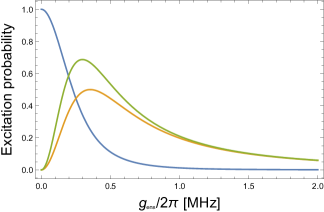
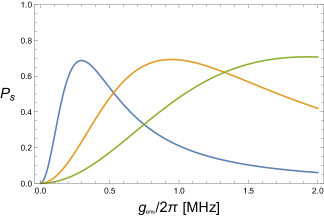
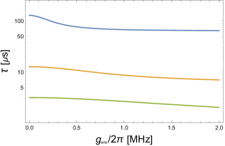
The excitation probability of the spin ensemble reads

$$P_{s}=\sum^{N}_{i=1}|\Psi^{(i)}_{s}(t)|^{2}=$$

$$=\int^{\infty}_{-\infty}\,d\Delta\int^{\infty}_{-\infty}\,dgp_{1}(\Delta)p_{2}(g)|\Psi_{s}(\Delta,g,t)|^{2}$$

$$=\frac{4g^{2}_{\text{ens}}w}{(\kappa_{\text{min}}+w)(4g^{2}_{\text{ens}}+\kappa_{\text{min}}w)},$$ (35)

where

$$\Psi_{s}(\Delta,g,t)=\frac{ge^{-i\Delta(t-t_{0})}(4\Delta+2iw)}{(2\Delta+iw)(2\Delta+i\kappa_{\text{min}})-4g^{2}_{\text{ens}}}.$$

The formula in (35) gives the maximum amount of excitation probability and can also be expressed as a function of the cooperativity $C=4g^{2}_{\text{ens}}/(\kappa_{\text{min}}w)$

$$P_{s}=\frac{C}{(1+C)(1+\kappa_{\text{min}}/w)},$$

which in the useful limiting case $w\gg\kappa_{\text{min}}$ yields $P_{s}=C/(1+C)$. In this limit, we want $C$ as high as possible. In this state the cavity is empty and the photon is found in the external field with $1-P_{s}$ probability. It is worth noting that (35) is equal to one, when $\kappa_{\text{min}}=0$, i.e., the photon cannot escape the cavity.

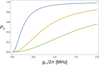
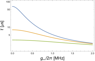
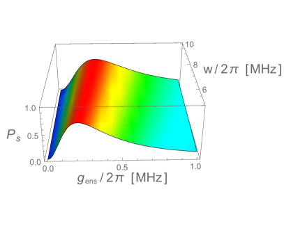
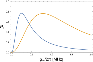
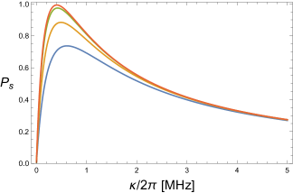
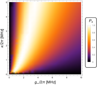
In Fig. 2 it is shown how the excitation probability of the spin ensemble in (35) changes for different values of $g_{\text{ens}}$ and $\kappa_{\text{min}}$. We have also plotted the required time to reach these values of the excitation probability. There is a tradeoff between getting high probabilities and reaching them as fast as possible, see for example the blue and the green curves in Fig. 2. We have argued earlier for a fast enough protocol to avoid population and phase decays of the spins and therefore the consistency of (35) has to be always examined for given experimental values of the parameters. In general, larger ensemble-coupling constants yield higher probabilities, while $\kappa_{\text{min}}$ and $w$ have destructive effects on the catch of the photon by the spin ensemble. According to Fig. 2, large values of $g_{\text{ens}}$ not only yield perfect absorption of the photon but also a fast protocol. Fig. 3 shows the dependence of the excitation probability $P_{s}$ on the width of the inhomogeneous broadening $w$; as the value of $w$ is decreasing $P_{s}$ is slightly increased. Inhomogeneous broadening of the spin ensemble is always an obstacle from the point of view of controllability, but here the two-step protocol has a reduced impact on the excitation storage.

Figure 3: Two-step protocol. Excitation probability of the spin ensemble as a function of the ensemble-coupling constant $g_{\text{ens}}$ and the width of the inhomogeneous broadening $w$; see Eq. (35). The decay rate of the cavity is set to $\kappa/2\pi=25$ kHz.

IV.3 Gaussian and other distributions of detunings

To demonstrate how the results from above can be generalized to arbitrary distributions of the inhomogeneous broadening of the spins, we first consider a Gaussian broadened spin ensemble

$$p_{1}(\Delta)=\frac{1}{\sqrt{2\pi}w}e^{-\Delta^{2}/(2w^{2})}.$$ (36)

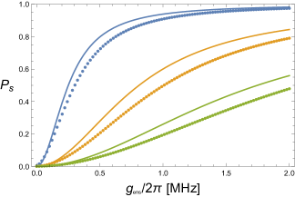
Based on the method described in Appendix A, we approximate this probability distribution with the sum of eight Lorentzian-shaped functions. These functions enable us to find numerically the poles required for the analytical evolution of the inverse Laplace transform. The results are presented in Fig. 4. The excitation probability of the Gaussian broadened spin ensemble is slightly smaller, but, in general, both distributions deliver the same features of photon absorption.

The same process can be repeated for other distributions of spins by matching the spectrum with what is empirically observed. In typical experiments, the distribution may have somewhat arbitrary broadening, including potentially multimodal distributions. For situations that differ significantly from Lorentzians or Gaussians, the approximation method here can still give closed form solutions to the temporal dynamics.

Figure 4: Two-step protocol with Lorentzian (solid) and Gaussian (dotted) broadened spin ensembles. Excitation probability of the spin ensemble as a function of the ensemble-coupling constant $g_{\text{ens}}$. All parameters and settings correspond to those of Fig. 2.

V One step, direct photon absorption

In this scenario, we investigate the possibility of direct absorption of the photon by the spin ensemble, i.e., the interaction between the single-mode cavity field and the spins is never turned off. Thus, the central spin frequency is equal for all times to the frequency of the single-mode field, which means that $\Delta_{cs}=0$. We first consider the one-step protocol as a special case of the two-step protocol. We then consider analytically derivable pulse shapes and finally at Gaussian pulses and optimal-control pulses. The optimized pulsed shapes will allow us to find also respective optimal values for the decay rate $\kappa$. Based on the model of Sec. II the main coupled differential equations are

$$\dot{\Psi}^{(i)}_{s} = i(\Delta_{N}-\Delta_{i})\Psi^{(i)}_{s}-ig_{i}\Psi_{c},$$

$$\dot{\Psi}_{c} = -g^{2}_{\text{ens}}\int^{t}_{0}e^{-w(t-t^{\prime})/2}\Psi_{c}(t^{\prime})\,dt^{\prime}+f(t)-\frac{\kappa}{2}\Psi_{c}.$$

If $\kappa$ is considered to be constant, then the solution for $\Psi^{(i)}_{s}$ reads

$$\Psi^{(i)}_{s}(t)=g_{i}\int^{t}_{0}\,dt^{\prime}f(t^{\prime})\left\{Ae^{-\frac{\kappa+w}{4}(t-t^{\prime})}\cosh\left[\frac{\varpi^{\prime}}{4}(t-t^{\prime})\right]\right.$$

$$+\left.Be^{-\frac{\kappa+w}{4}(t-t^{\prime})}\sinh\left[\frac{\varpi^{\prime}}{4}(t-t^{\prime})\right]-Ae^{i(\Delta_{N}-\Delta_{i})(t-t^{\prime})}\right\},$$

(37)

where

$$A = \frac{4\Delta_{N}-4\Delta_{i}-2iw}{(2\Delta_{i}-2\Delta_{N}+iw)(2\Delta_{i}-2\Delta_{N}+i\kappa)-4g^{2}_{\text{ens}}},$$

$$B = \frac{1}{\varpi^{\prime}}\frac{(4\Delta_{N}-4\Delta_{i}-2iw)(w-\kappa)+16ig^{2}_{\text{ens}}}{(2\Delta_{i}-2\Delta_{N}+iw)(2\Delta_{i}-2\Delta_{N}+i\kappa)-4g^{2}_{\text{ens}}}.$$

V.1 Exponential shape pulse

In this subsection, we demonstrate that the one-step and two-step protocols are markedly different. To understand the situation better we consider

$$f(t)=\kappa H(t_{0}-t)e^{\kappa(t-t_{0})/2},$$ (38)

which is the ideal solution for the two-step protocol with $\Delta_{cs}=0$, see Eq. (29). This choice guarantees that the single-mode cavity field is perfectly excited at $t=t_{0}$. Therefore, we have evaluated in this one-step protocol the excitation probability of the cavity field at $t=t_{0}$ and a lengthy calculation involving the integration over the detunings of the spin ensemble with the Lorentzian weight $p_{1}(\Delta)$ yields

$$|\Psi_{c}(t_{0})|^{2}=\frac{\kappa^{2}(\kappa+w)^{2}}{\left[2g^{2}_{\text{ens}}+\kappa(\kappa+w)\right]^{2}}.$$ (39)

Similarly, the excitation is in the spin ensemble with probability:

$$P_{s}(t_{0})=\sum^{N}_{i=1}|\Psi^{(i)}_{s}(t_{0})|^{2}=\frac{4g^{2}_{\text{ens}}\kappa(\kappa+w)}{\left[2g^{2}_{\text{ens}}+\kappa(\kappa+w)\right]^{2}}.$$ (40)

Both formulas are valid under the assumption $\kappa t_{0}/2\gg 1$ or $e^{-\kappa t_{0}/2}\approx 0$.

If we consider a long enough interaction time $t$ such that $\operatorname{Re}[\kappa+w-\varpi^{\prime}](t-t_{0})/4\gg 1$, then $\Psi_{c}(t)\approx 0$ and the excitation probability of the spin ensemble is

$$P_{s}=\sum^{N}_{i=1}|\Psi^{(i)}_{s}(t)|^{2}=\int^{\infty}_{-\infty}d\Delta\,p_{1}(\Delta)$$ (41)

$$\times\frac{16g^{2}_{\text{ens}}\kappa^{2}(4\Delta^{2}+w^{2})}{(4\Delta^{2}+\kappa^{2})\left[4\Delta^{2}(\kappa+w)^{2}+(4g^{2}_{\text{ens}}+\kappa w-4\Delta^{2})^{2}\right]}.$$

It is worth noting that the above integration can be analytically done, however it yields cumbersome formulas, which are not worth being presented.

Figure 5: One-step protocol with $f(t)$ in Eq. (38). Excitation probabilities of the spin ensemble and the single-mode cavity field as a function of the ensemble-coupling constant $g_{\text{ens}}$. The width of the inhomogeneous broadening is set to $w/2\pi=10$ MHz and $\kappa/2\pi=25$ kHz. The curves show different probabilities: the cavity field is excited at $t=t_{0}$, see Eq. (39) (blue); the spin ensemble absorbed the excitation at $t=t_{0}$, see Eq. (40) (orange); the spin ensemble absorbed the excitation after a longer interaction time, when the cavity is empty, see Eq. (41) (green).

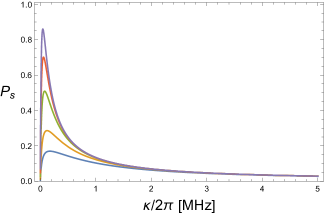
The choice of $f(t)$ or indirectly the choice of the initial conditions of the external field results in a surprising effect, a larger ensemble-coupling constant $g_{\text{ens}}$ does not necessarily imply better excitation probabilities $P_{s}$ of the spin ensemble and for very large values of $g_{\text{ens}}$ the probability of storing the excitation is reduced to zero. This limiting case for high values of $g_{\text{ens}}$ from (41) yields $P_{s}=\kappa w/g^{2}_{\text{ens}}+O(1/g^{3}_{\text{ens}})$. This is apparent from Fig. 5. The single-mode of the cavity can be perfectly excited at $g_{\text{ens}}=0$ and $P_{s}$ reaches its maximum after the cavity is empty and only for a given value of $g_{\text{ens}}$. This value is increased with the increase of $\kappa$. This repulsive character of the joint system of the cavity field and the spin ensemble is very different from the results obtained for the two-step protocol; see Fig. 2. For comparison, we show the results for the exponential pulse for the one-step protocol in Fig. 6. The one-step protocol performs better for low values of $g_{\text{ens}}$, but it requires longer times to reach better excitation probabilities of the spin ensemble. For shorter protocols, a larger $\kappa$ is needed, but then the maximum of the probability is shifted towards larger values of $g_{\text{ens}}$. Whether a faster protocol or better absorption of the incoming photon is preferred, depends on the experimental setup and the planned further control of the spin ensemble, e.g., the application of $\pi$ pulses to refocus the spin dephasing. A reduced value of the inhomogeneous broadening $w$ shifts the maximum of $P_{s}$ towards smaller values of $g_{\text{ens}}$; see Fig. 7. This is not surprising, because larger $w$s mean more far-detuned spin transitions, which limit the storage of the photon in the spin ensemble.

Figure 6: One-step protocol with $f(t)$ in Eq. (38). Top panel: Excitation probability of the spin ensemble as a function of the ensemble-coupling constant $g_{\text{ens}}$. Bottom panel: Semilogarithmic plot of the required time $\tau$ of the protocols to reach the maximum excitation probability. All parameters and settings correspond to those of Fig. 2, with as before the lines corresponding to $\kappa_{\text{min}}/2\pi=25$ kHz (blue), $\kappa_{\text{min}}/2\pi=250$ kHz (orange), and $\kappa_{\text{min}}/2\pi=1$ MHz (green).

Figure 7: One-step protocol with $f(t)$ in Eq. (38). Excitation probability of the spin ensemble as a function of the ensemble-coupling constant $g_{\text{ens}}$ and the width of the inhomogeneous broadening $w$; see Eq. (41). The decay rate of the cavity is set to $\kappa/2\pi=25$ kHz.

V.2 Analytically derivable pulse shape

As we have demonstrated, reusing the exponential pulse $f(t)$ derived for the two-step protocol is not a pracitical choice to store the excitation in the spin ensemble in one step. Therefore, in the subsequent discussion, we investigate further candidates, which lead to more optimal storage. First, we rewrite Eq. (37) as

$$\Psi^{(i)}_{s}(t)=g_{i}\int^{t}_{0}\,dt^{\prime}f(t^{\prime})h_{i}(t^{\prime},t),$$

where the integral kernel $h_{i}(t^{\prime},t)$ is implicitly defined via Eq. (37). The excitation probability of the spin ensemble at time $T$ reads

$$P_{s}=\sum^{N}_{i=1}|\Psi^{(i)}_{s}(T)|^{2}=\sum^{N}_{i=1}g^{2}_{i}\left|\int^{T}_{0}\,dt^{\prime}f(t^{\prime})h_{i}(t^{\prime},T)\right|^{2}$$

$$=g^{2}_{\text{ens}}\int^{\infty}_{-\infty}d\Delta\,p_{1}(\Delta)\left|\int^{T}_{0}\,dt^{\prime}f(t^{\prime})h(t^{\prime},T,\Delta)\right|^{2},$$ (42)

with

$$h(t^{\prime},T,\Delta)=A(\Delta)e^{-\frac{\kappa+w}{4}(T-t^{\prime})}\cosh\left[\frac{\varpi^{\prime}}{4}(T-t^{\prime})\right]$$

$$+B(\Delta)e^{-\frac{\kappa+w}{4}(T-t^{\prime})}\sinh\left[\frac{\varpi^{\prime}}{4}(T-t^{\prime})\right]-A(\Delta)e^{-i\Delta(T-t^{\prime})}$$

and

$$A(\Delta) = \frac{-4\Delta-2iw}{(2\Delta+iw)(2\Delta+i\kappa)-4g^{2}_{\text{ens}}},$$

$$B(\Delta) = \frac{1}{\varpi^{\prime}}\frac{(-4\Delta-2iw)(w-\kappa)+16ig^{2}_{\text{ens}}}{(2\Delta+iw)(2\Delta+i\kappa)-4g^{2}_{\text{ens}}}.$$

Figure 8: Optimized one-step protocol with $f(t)$ in Eq. (43). Top panel: Excitation probability of the spin ensemble as a function of the ensemble-coupling constant $g_{\text{ens}}$. The curves belong to different values of $\kappa$: $\kappa/2\pi=25$ kHz (blue) and $\kappa/2\pi=250$ kHz (orange). Bottom panel: The optimal $f(t)$ as a function of time, where $T=20\mu$s and $\kappa/2\pi=25$ kHz. The width of the inhomogeneous broadening is set to $w/2\pi=10$ MHz. In the numerical evaluation, we have considered that $e^{-5}\approx 0$.

We observe that $h(t^{\prime},T,\Delta)\in L^{2}\left([0,T]\right)$, i.e. $h$ is a square-integrable function on the interval $[0,T]$. The function space $L^{2}\left([0,T]\right)$ is a Hilbert space with the inner product Yosida (1995)

$$\langle f,h\rangle=\int^{T}_{0}\,dt^{\prime}f(t^{\prime})\overline{h}(t^{\prime}),$$

where $\overline{z}$ denotes the complex conjugate of a complex number $z$. In the case of this particular inner product, the Cauchy-Bunyakovsky-Schwarz inequality reads

$$\left|\int^{T}_{0}\,dt^{\prime}f(t^{\prime})\overline{h}(t^{\prime})\right|^{2}\leqslant\int^{T}_{0}\,dt^{\prime}|f(t^{\prime})|^{2}\int^{T}_{0}\,dt^{\prime}|h(t^{\prime})|^{2},\\$$

where the equality occurs if and only if one of $h(t^{\prime})$, $f(t^{\prime})$ is a scalar multiple of the other. However, in Eq. (42) we have a $\Delta$-dependent family of inner products of the form $\langle f,h(\Delta)\rangle$ and their squared absolute values are integrated over all $\Delta$ with the weight function $p_{1}(\Delta)$. Thus, the Cauchy-Bunyakovsky-Schwarz inequality can be applied for each value of $\Delta$, which results in a $\Delta$-dependent $f(t^{\prime})$, i.e., multiple optimal solutions and they depend on the detunings of the individual spins. Instead, we consider only one optimal solution at the maximum $\Delta=0$ of the weight function $p_{1}(\Delta)$ in (15) and arrive at

$$f(t)=\lambda\left\{a-ae^{-\frac{\kappa+w}{4}(T-t)}\cosh\left[\frac{\varpi^{\prime}}{4}(T-t)\right]\right.$$

$$+\left.be^{-\frac{\kappa+w}{4}(T-t)}\sinh\left[\frac{\varpi^{\prime}}{4}(T-t)\right]\right\},$$ (43)

where by absorbing the imaginary unit into $\lambda$ we get

$$a = \frac{2w}{w\kappa+4g^{2}_{\text{ens}}},$$

$$b = \frac{1}{\varpi^{\prime}}\frac{2w(w-\kappa)-16g^{2}_{\text{ens}}}{w\kappa+4g^{2}_{\text{ens}}}.$$

The parameter $\lambda$ is found from the normalization condition. In order to do so, we determine the normalization of Eq. (38), which reads

$$\int^{T}_{0}\,dt\,\left|\kappa H(t_{0}-t)e^{\kappa(t-t_{0})/2}\right|^{2}=\kappa,$$

where we have used $T\geqslant t_{0}$ and $e^{-\kappa t_{0}/2}\approx 0$. The physical meaning of this normalization is that the input field contains exactly one photon. A more detailed discussion of this constraint is presented in Appendix B. Now, we set the normalization of Eq. (43) to $\kappa$, i.e.,

$$\int^{T}_{0}\,dt|f(t)|^{2}=\kappa.$$ (44)

We consider again a long enough interaction time $T$ such that $\operatorname{Re}[\kappa+w-\varpi^{\prime}]T/4\gg 1$. In Fig. 8, we see the same behavior of the excitation probabilities, which we have observed in Fig. 5, i.e., there is a maximum only for a given value of the ensemble-coupling constant $g_{\text{ens}}$. However, the curves in Fig. 6 reach a maximum value of $0.7$, whereas now the excitation probability has a maximum larger than $0.75$. For the case of $\kappa/2\pi=25$ kHz, the optimal $f(t)$ is also displayed in Fig. 8. The required times to reach these excitation probabilities are the same as the ones depicted in Fig. 6. The role of the inhomogeneous broadening $w$ is the same as what we have observed for the previous $f(t)$ in Eq. (38); see again Fig. 7.

Figure 9: Excitation probability $P_{s}$ of the spin ensemble as a function of cavity decay rate $\kappa$ with with $g_{\text{ens}}/2\pi=1$ MHz (top panel) and $g_{\text{ens}}/2\pi=0.3$ MHz (middle panel). We set $\kappa_{g}$ in Eq. (45) as: $\kappa_{g}/2\pi=500$ kHz (blue); $\kappa_{g}/2\pi=250$ kHz (orange); $\kappa_{g}/2\pi=100$ kHz (green); $\kappa_{g}/2\pi=50$ kHz (red); and $\kappa_{g}/2\pi=25$ kHz (purple). Bottom panel: Density plot of $P_{s}$ as a function of $\kappa$ and $g_{\text{ens}}$ for $\kappa_{g}/2\pi=50$ kHz. The width of the inhomogeneous broadening is set for all figures to $w/2\pi=10$ MHz.

V.3 Gaussian pulse shape

(a) Gaussian pulse shapes

(b) Optimized pulse shapes

Figure 10: Excitation probability of the spin ensemble $P_{s}$ as a function of the cavity decay rate $\kappa$ and ensemble-coupling constant $g_{\text{ens}}$ for Gaussian (a) and optimized (b) pulse shapes. We consider for both figures $\omega/2\pi=10$ MHz and $T=20\mu$s. To highlight the higher values of $P_{s}$ for the optimized pulse shapes, we show in both plots a white dot at $g_{\text{ens}}/2\pi=350$ kHz and $\kappa=50$ kHz corresponding to a cooperativity of $C=0.98$ and observe an increase of $0.19$ in the value of excitation probability.

Finally, we investigate a widely used case when $f(t)$ is a Gaussian function, which can benefit from favourable bandwidth considerations Ranjan et al. (2020):

$$f(t)=\frac{\sqrt{\kappa\kappa_{g}}}{\pi^{\nicefrac{{1}}{{4}}}}e^{-\kappa^{2}_{g}(t-t_{0})^{2}/2},$$ (45)

where $\nicefrac{{1}}{{\kappa_{g}}}$ is the standard deviation of the pulse. If $t_{0}\gg\nicefrac{{1}}{{\kappa_{g}}}$, then it is immediate that $\int^{\infty}_{0}\,dt|f(t)|^{2}=\kappa$. We substitute (45) into Eq. (37) with both conditions $T>t_{0}$ and

$$\operatorname{Re}\left[\frac{\kappa+w\pm\varpi^{\prime}}{4}(T-t_{0})-\frac{\left(\kappa+w\pm\varpi^{\prime}\right)^{2}}{32\kappa^{2}_{g}}\right]\gg 1$$ (46)

being fulfilled. The latter condition is necessary for the approximation, where all $\Delta$-independent exponential terms are considered to be zero. Based on this, the excitation probability $P_{s}$ of the spin ensemble is obtained as before by replacing the summation over the spins with an integral involving the joint distribution $p_{1}(\Delta)p_{2}(g)$ and yields

$$P_{s}=\int^{\infty}_{-\infty}d\Delta\,p_{1}(\Delta)\frac{2\kappa\sqrt{\pi}}{\kappa_{g}}e^{-\frac{\Delta^{2}}{\kappa^{2}_{g}}}$$ (47)

$$\times\frac{4g^{2}_{\text{ens}}(4\Delta^{2}+w^{2})}{\left[4\Delta^{2}(\kappa+w)^{2}+(4g^{2}_{\text{ens}}+\kappa w-4\Delta^{2})^{2}\right]}.$$

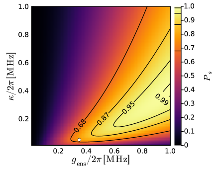
In the first step, we investigate the width of the Gaussian and find numerically that optimal scenarios occur when the bandwidth $\kappa_{g}$ is as small as possible, see Fig. 9. In this figure, it is also demonstrated that perfect excitations are achieved for different decay rates of the cavity as a function of the ensemble-coupling $g_{\text{ens}}$. The repulsive behavior of excitation probability $P_{s}$ as a function of $g_{\text{ens}}$ is similar to the previous cases of the one-step protocol. The duration of the process depends on the standard deviation of the pulse $\sigma_{g}=\nicefrac{{1}}{{\kappa_{g}}}$ and the condition in (46). First, $t_{0}>3\sigma_{g}$ and $T>6\sigma_{g}$ have to be valid such that the integration over time covers almost the whole pulse. In the case of $\nicefrac{{\kappa_{g}}}{{2}}\pi=50$ kHz, $\nicefrac{{\kappa}}{{2}}\pi=0.5$ MHz, $\nicefrac{{g_{\text{ens}}}}{{2}}\pi=1$MHz, and $\nicefrac{{w}}{{2\pi}}=10$ MHz, we obtain $T>161.8\mu$s provided that $e^{-5}\approx 0$. Thus, perfect excitation is possible at the expense of an increase in the duration of the protocol. This is much longer than the duration times obtained for the two-step protocol, see Fig. 2, where this set of parameters yields $T>3.28\mu$s. This raises the question of how can one obtain perfect excitation for considerably shorter times, which will be discussed in the subsequent section devoted to numerical analysis.

V.4 Optimal control - numerically optimized pulse shapes

We now turn our attention to the numerical optimization for pulse shapes $f(t)$, decay rate of the cavity $\kappa$, and pulse durations $T$ to overcome the limitations of the previous attempts. In order to optimize constrained pulse shapes $f(t)$ (see. Eq. (44)) with otherwise given parameters

$$f_{\text{opt}}=\underset{f}{\operatorname{argmax}}\,P_{s}\left(f,T,w,g_{\text{ens}},\kappa\right),$$ (48)

we expand $f(t)$ in a set of basis functions $f(t)=\sum_{j=0}^{2N_{b}}c_{j}f_{j}(t)$, where

$$f_{j}(t)=\begin{cases}\cos\left(\pi\frac{jt}{T}\right)&\text{for }0\leqslant j\leqslant N_{b},\\ \sin\left(\pi\frac{(j-N_{b})t}{T}\right)&\text{for }N_{b}<j\leqslant 2N_{b}.\end{cases}$$ (49)

We have $N_{b}+1$ cosine terms, with $f_{0}(t)=1$ being a constant term and $N_{b}$ sine terms. In some experimental setups Ranjan et al. (2022), $\kappa$ can be adjusted, so we extend our approach to also optimize $\kappa$

$$\kappa_{\text{opt}}=\underset{\kappa}{\operatorname{argmax}}\,P_{s}(f_{\text{opt}}(\kappa),T,w,g_{\text{ens}},\kappa).$$ (50)

Using the subsequent optimization of pulse shape $f(t)$ and $\kappa$, we can also determine the shortest pulse duration $T_{\text{min}}$ needed to achieve a target excitation probability $P_{s,\text{tar}}$. This is accomplished by identifying the root of the equation

$$\Delta P_{s,\text{tar}}(T)=P_{s,\text{tar}}-P_{s}(f_{\text{opt}}(\kappa),T,w,g_{\text{ens}},\kappa_{\text{opt}}),$$ (51)

where $\Delta P_{s,\text{tar}}(T)$ represents the deviation from the target excitation probability. The condition $\Delta P_{s,\text{tar}}(T_{\text{min}})=0$ is sufficient for finding the minimum duration since we investigate a regime where the absorption is increasing monotonically with $T$.

We combine analytical and numerical techniques to solve Eq. (42) restated for a set of basis functions, which allows us to solve the optimization problems in Eqs. (48 - 51). The technical details of both optimization and numerical integration are explained in Appendix C. The numerical approach was implemented using the Julia language Bezanson et al. (2017), our code is available atBernád .

Figure 11: Optimal and Gaussian pulse shape for $g_{\text{ens}}/2\pi=0.5$ MHz, $T=10\mu$s, $w/2\pi=10$ MHz and the optimized $\kappa/2\pi\approx 0.121$ MHz. For the Gaussian we set $\kappa_{g}=\nicefrac{{2\pi}}{{T}}$. We achieve an excitation probability of $P_{s}=0.88$ for the optimized and $0.78$ for the Gaussian pulse shapes.

Figure 12: Optimal cooperativity $C=4g_{\text{ens}}^{2}/(\kappa w)$ as a function of $g_{\text{ens}}$ and $T$ at $w/2\pi=10$ MHz.

(a) Time to reach target $P_{s,\text{tar}}$ for optimized pulse shapes.

(b) Speedup of optimized pulse shapes.

Figure 13: (a) Logarithm of the time required to reach a target $P_{s,\text{tar}}$ value as a function of $g_{\text{ens}}$ and (b) the corresponding speedup of optimized pulse shapes over Gaussians using $w/2\pi=10$ MHz and individually optimized $\kappa$ values.

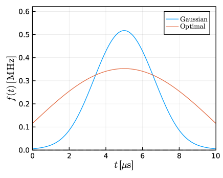
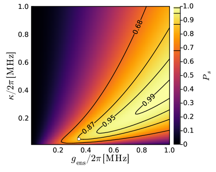
Results. In the previous section, we have demonstrated that the Gaussian pulse shapes under the condition of long pulse duration can achieve almost perfect excitation probabilities $P_{s}$. Now, we compare the bottom panel in Fig. 9 with the results of the optimized pulse shapes. In Fig. 10, it is demonstrated that our optimization approach yields a better performance. This time, instead of direct numerical integration, we first expand the Gaussian function into the first eleven basis functions, i.e., $N_{b}=5$ in Eq. (49). This is a sufficiently accurate approximation, granting a relative error smaller than $1\%$ (and in tests comparing $N_{b}=5$ to $N_{b}=10$ giving 4 significant digits) and allows us to reuse the methodology based on $\mathbf{c}$. An optimized pulse is presented in Fig. 11 and compared to its Gaussian counterpart of Eq. (45) with $\kappa=\kappa_{g}$. Initially, we run our optimizations with $N_{b}=5$. In doing so, we find for all optimizations, that optimal pulses depend only on the constant ($j=0$), the first cosine term ($j=1$), and the first sine term ($j=N_{b}+1$) in Eq. (49). Thus, we find an optimal pulse

$$f(t)=A\sin\left(\frac{\pi t}{T}+\phi\right),$$ (52)

where the variable $A$ is fixed by the normalization of Eq. (44), while $\phi$ is numerically determined. This has motivated a cut-off for the optimizations using only $N_{b}=1$, because increasing $N_{b}$ to five makes only an order of $~{}10^{-9}$ difference in $P_{s}$, comparable to our numerical integration error.

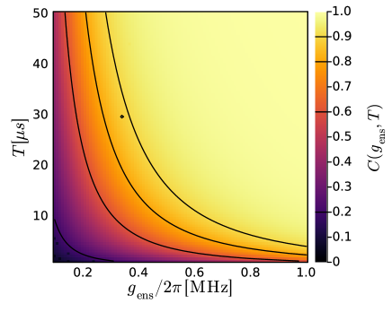
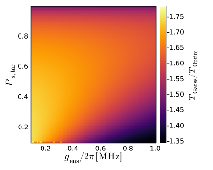
In Fig. 12, we show the optimal cooperativity $C=4g_{\text{ens}}^{2}/(\kappa w)$ as a function of $g_{\text{ens}}$ and $T$. This reproduces previous results of Ref. Afzelius et al. (2013) suggesting, that for large times $T$ and coupling strengths $g_{\text{ens}}$, the ideal cooperativity takes the value $1.0$. However, for current experimental setups Ranjan et al. (2022) $g_{\text{ens}}=350$ kHz and $T$ is at most $10\mu$s, which suggests that optimal excitation probability is achieved for values of $C$ between $0.6$ and $0.7$. It is worth noting that for given values of $g_{\text{ens}}$ and $T$ and optimized $\kappa$ the optimal excitation probability may not be equal to one. Finally, we focus on a different perspective: for optimized values of $\kappa$ and a target excitation probability, how does the pulse duration $T$ depend on given values of $g_{\text{ens}}$. Our findings in Fig. 13 demonstrate if $g_{\text{ens}}$ is not large enough then this can be only compensated by larger values of $T$. As higher is the target excitation probability, more demanding are the conditions for both $g_{\text{ens}}$ and $T$. We have also compared in Fig. 13 the required time for a Gaussian and an optimized pulse shape. We find an approximately $1.7$-fold speedup over the Gaussian pulses for the experimentally relevant regime with $\nicefrac{{g_{\text{ens}}}}{{2\pi}}\in[0.2,0.4]\,\text{MHz}$, and limited dependence on $P_{s}$. For the highest target values of $P_{s}$, the speedup decreases slightly, this might be an artifact due to limitations in the root finding precision for exceedingly long pulse durations $T$.

VI Summary and conclusions

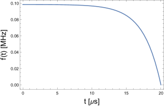
In the context of optimal photon storage in a spin-ensemble-based quantum memory, we have presented a minimal model capable of describing the physics of such a system. We have shown the analytical solutions of the time evolution and the required approximations. Based on these results we have proposed a two-step and several one-step protocols. By using parameters corresponding to current experiments, we have found several pros and cons of the proposed protocols. The two-step protocol can achieve almost perfect absorption of the photon, but this happens for large values of ensemble-coupling $g_{\text{ens}}$. The one-step protocols can achieve good absorption probabilities for lower values of $g_{\text{ens}}$ and in the case of Gaussian pulses with a broad temporal profile one can obtain perfect absorption. The maximum is reached for certain values of $\kappa$ and $g_{\text{ens}}$. Furthermore, the one-step protocols are characterized by a repulsive character, i.e., a too large ensemble-coupling prevents the photon from being absorbed. In general, as one would expect, we have observed that low values of the cavity decay and the line width of the inhomogeneous broadening $w$ improve the success of the protocols. Finally, numerical optimizations of the pulse shapes have resulted in shorter protocol times and higher absorption probabilities of the photon. This has also motivated a new pulse shape, a half-period sine pulse shifted upwards (Fig. 11), which can speed up absorption.

In conclusion, our theoretical search for optimal storage of a photon serves as a prerequisite for more advanced tasks, such as storing quantum states in a long-time memory or reobtaining the state by using the Hahn echo Hahn (1950). Optimal storage of quantum information brings promise also for applications such as entanglement purification in quantum repeaters or atomic clocks.

Appendix A Gaussian distribution of the broadened spin ensemble

In the main text, we have mainly considered a Cauchy-Lorentz distribution and now we show the details concerning a Gaussian probability distribution in Eq. (36). Then, we have

$$\Delta_{N}=\sum^{N}_{i=1}\frac{\Delta_{i}}{2}\rightarrow\int^{\infty}_{-\infty}p_{1}(\Delta)\frac{\Delta}{2}\,d\Delta=0$$ (53)

and

$$\sum^{N}_{i=1}e^{i(\Delta_{N}-\Delta_{i})(t-t^{\prime})}\rightarrow\int^{\infty}_{-\infty}\,p_{1}(\Delta)e^{-i\Delta(t-t^{\prime})}d\Delta$$

$$=e^{-w^{2}(t-t^{\prime})^{2}/2}.$$ (54)

Thus, Eq. (14) with $\Delta_{cs}=0$ reads

$$\dot{\Psi}_{c}=-g^{2}_{\text{ens}}\int^{t}_{0}e^{-w^{2}(t-t^{\prime})^{2}/2}\Psi_{c}(t^{\prime})\,dt^{\prime}+f(t)-\frac{\kappa}{2}\Psi_{c}.$$ (55)

A general solution to this equation can be obtained with the help of the Laplace transformation

$$\Psi_{c}(z)=\int^{\infty}_{0}\Psi_{c}(t)e^{-zt}\,dt.$$ (56)

We use the properties of the Laplace transform on Eq. (55) to obtain

$$-\Psi_{c}(0)+z\Psi_{c}(z) = -g^{2}_{\text{ens}}\frac{\sqrt{\frac{\pi}{2}}e^{\frac{z^{2}}{2w^{2}}}\operatorname{erfc}\left(\frac{z}{\sqrt{2}w}\right)}{w}\Psi_{c}(z)$$ (57)

$$+ f(z)-\frac{\kappa}{2}\Psi_{c}(z),$$

where $\operatorname{erfc}$ is the complementary error function. The solution is

$$\Psi_{c}(z)=\frac{\Psi_{c}(0)}{P(z)}+\frac{f(z)}{P(z)}$$ (58)

with

$$P(z)=z+\frac{\kappa}{2}+g^{2}_{\text{ens}}\frac{\sqrt{\frac{\pi}{2}}e^{\frac{z^{2}}{2w^{2}}}\operatorname{erfc}\left(\frac{z}{\sqrt{2}w}\right)}{w}.$$ (59)

To evaluate the inverse Laplace transform, one needs to solve $P(z)=0$, which is a transcendental equation and has only approximate numerical solutions. In fact, all of them have to be found to obtain the solution to Eq. (55). Instead of searching on the whole complex plane, one can approximate the Gaussian distribution in (36) as

$$p_{1}(\Delta)\approx\frac{1}{\sqrt{2\pi}w}\sum^{M_{1}}_{i=1}\frac{a_{i}}{b_{i}+\Delta^{2}},$$ (60)

where $a_{i},b_{i}\in\mathbb{R}$ and $b_{i}\geqslant 0$ for all $i$.

We implement the gradient descent method Boyd and Vandenberghe (2004) by using $M_{2}$ points to discretize $p_{1}(\Delta)$. At each point $\Delta_{j}$, we compute the squared distance between the actual function value and the estimated function value. Finally, we sum up all terms to obtain the cost function

$$C=\sum^{M_{2}}_{j=1}\left(p_{1}(\Delta_{j})-\frac{1}{\sqrt{2\pi}w}\sum^{M_{1}}_{i=1}\frac{a_{i}}{b_{i}+\Delta^{2}_{j}}\right)^{2}.$$ (61)

Now, we use the update equations:

$$a_{i}-\gamma\pdv{C}{a_{i}}\to a_{i}\quad\text{and}\quad b_{i}-\gamma\pdv{C}{b_{i}}\to b_{i},$$ (62)

where $\gamma$ is the learning rate. This approach leads to a different Laplace transformed equation:

$$-\Psi_{c}(0)+z\Psi_{c}(z) = -g^{2}_{\text{ens}}\sum^{M_{1}}_{i=1}\frac{a_{i}}{w}\sqrt{\frac{\pi}{2b_{i}}}\frac{1}{\sqrt{b_{i}}+z}\Psi_{c}(z)$$ (63)

$$+ f(z)-\frac{\kappa}{2}\Psi_{c}(z),$$

see Eq. (57) for a comparison. In place of (59), we have

$$P(z)=z+\frac{\kappa}{2}+g^{2}_{\text{ens}}\sum^{M_{1}}_{i=1}\frac{a_{i}}{w}\sqrt{\frac{\pi}{2b_{i}}}\frac{1}{\sqrt{b_{i}}+z}$$ (64)

and $P(z)=0$ results in a problem, where the roots of a $(M_{1}+1)$th degree polynomial have to be determined. Numerically, this is a simpler task than solving a transcendental equation, because we have to find exactly $(M_{1}+1)$ roots.

Appendix B Constraint on the pulse shapes in one-step protocols

The pulse shape $f(t)$ acts as an external drive and depends only on the properties of the external field and their couplings to the single-mode field inside the cavity (see Eq. (12)). The probability amplitude $\Psi_{c}$ of the single-mode in the cavity is governed by Hamiltonian dynamics, however, after the Weisskopf-Wigner approximation is subject to decay. In this approximated theory, the question is what are the properties of $f(t)$ such that $\Psi_{c}$ remains a probability amplitude? This issue is not related to the spin ensemble and its interaction with the single-mode field. Therefore, we start with the differential equations

$$\dot{\Psi}_{c} = -i\sum_{j\in L}\kappa^{*}_{j}\Psi^{(j)}_{E},$$ (65)

$$\dot{\Psi}^{(j)}_{E} = -i\delta_{j}\Psi^{(j)}_{E}-i\kappa_{j}\Psi_{c}.$$ (66)

For the initial conditions, similarly to the main text, we assume that the excitation is in the external field

$$\Psi_{c}(0)=0,\quad\text{and}\quad\sum_{j\in L}|\Psi^{(j)}_{E}(0)|^{2}=1.$$ (67)

We have already solved this for $\Psi_{c}(t)$ in Eq. (9), which reads now

$$\dot{\Psi}_{c}=-i\sum_{j\in L}\kappa^{*}_{j}\Psi^{(j)}_{E}(0)e^{-i\delta_{j}t}$$ (68)

$$-\sum_{j\in L}|\kappa_{j}|^{2}\int^{t}_{0}e^{-i\delta_{j}(t-t^{\prime})}\Psi_{c}(t^{\prime})\,dt^{\prime}.$$

Now, as it is explained at Eq. (10), we replace the summation over the modes with an integral to have

$$\sum_{j\in L}|\kappa_{j}|^{2}\int^{t}_{0}e^{-i\delta_{j}(t-t^{\prime})}\Psi_{c}(t^{\prime})\,dt^{\prime}$$

$$=\int^{\infty}_{-\infty}d\delta\,\tilde{\rho}_{E}(\delta)|\kappa(\delta)|^{2}\int^{t}_{0}e^{-i\delta(t-t^{\prime})}\Psi_{c}(t^{\prime})\,dt^{\prime},$$

where we have introduced the density of states $\rho_{E}(\delta)$ instead of $\rho_{E}(\mathbf{k})$. This step allows us to get quicker to the property of $f(t)$ than using the integration over $\mathbf{k}$.

In the next step, we assume

$$\tilde{\rho}_{E}(\delta)|\kappa(\delta)|^{2}\approx\frac{\kappa}{2\pi},$$ (70)

i.e., this quantity varies little as a function of $\delta$. The integral

$$\int^{\infty}_{-\infty}\,d\delta\,e^{-i\delta(t-t^{\prime})}=\lim_{\epsilon\to 0}\int^{\infty}_{0}\,d\delta\,e^{-i\delta(t-t^{\prime})-\epsilon\delta}$$

$$+\lim_{\epsilon\to 0}\int^{0}_{-\infty}\,d\delta\,e^{-i\delta(t-t^{\prime})+\epsilon\delta}=2\pi\delta(t-t^{\prime}),$$ (71)

where $\epsilon>0$ and $\delta(t)$ is the Dirac delta function. Here, we have used the following representation of the Dirac delta function:

$$\delta(t-t^{\prime})=\lim_{\epsilon\to 0}\frac{1}{\pi}\frac{\epsilon}{(t-t^{\prime})^{2}+\epsilon^{2}}$$ (72)

Then, (B) reads

$$\frac{\kappa}{2\pi}2\pi\int^{t}_{0}\delta(t-t^{\prime})\Psi_{c}(t^{\prime})\,dt^{\prime}=\frac{\kappa}{2}\Psi_{c}(t),$$ (73)

because the integration from $0$ to $t$ covers only half of the function in (72), which is symmetrical about the $t=t^{\prime}$ vertical line.

We shall now extend this approximation to the external drive $f(t)$. From the general solution to Eq. (66) we find

$$f(t) = -i\sum_{j\in L}\kappa^{*}_{j}\Psi^{(j)}_{E}(0)e^{-i\delta_{j}t}$$ (74)

$$= -i\int^{\infty}_{-\infty}d\delta\,\tilde{\rho}_{E}(\delta)\kappa^{*}(\delta)\Psi_{E}(\delta,0)e^{-i\delta t}.$$ (75)

Furthermore, we have

$$1 = \sum_{j\in L}|\Psi^{(j)}_{E}(0)|^{2}=\int^{\infty}_{-\infty}d\delta\,\tilde{\rho}_{E}(\delta)|\Psi_{E}(\delta,0)|^{2}$$ (76)

$$= \int^{\infty}_{-\infty}d\delta\,|\tilde{\Psi}_{E}(\delta,0)|^{2},$$

where we have absorbed the square root of the positive function $\tilde{\rho}_{E}(\delta)$ into $\Psi_{E}(\delta,0)$. We need to assume that $\kappa^{*}_{j}$ for all $j$ or $\kappa^{*}(\delta)$ are real to introduce in (75) the following relation

$$\sqrt{\tilde{\rho}_{E}(\delta)}\kappa(\delta)=\frac{\sqrt{\kappa}}{\sqrt{2\pi}}$$ (77)

based on (70). Hence,

$$f(t)=-i\sqrt{\kappa}\underbrace{\frac{1}{\sqrt{2\pi}}\int^{\infty}_{-\infty}d\delta\,\tilde{\Psi}_{E}(\delta,0)e^{-i\delta t}}_{=\tilde{\Psi}_{E}(t,0)},$$ (78)

where $\tilde{\Psi}_{E}(t,0)$ is the Fourier transform of $\tilde{\Psi}_{E}(\delta,0)$. Then, we have

$$\int^{\infty}_{-\infty}|f(t)|^{2}\,dt=\kappa\int^{\infty}_{-\infty}|\tilde{\Psi}_{E}(t,0)|^{2}\,dt.$$ (79)

Now, we use Eq. (76) and Plancherel’s theorem Yosida (1995), which shows that the Fourier transform map is an isometry with respect to the $L^{2}$ norm:

$$\int^{\infty}_{-\infty}|\tilde{\Psi}_{E}(t,0)|^{2}\,dt=\int^{\infty}_{-\infty}|\tilde{\Psi}_{E}(\delta,0)|^{2}\,d\delta=1.$$ (80)

It is immediate

$$\int^{\infty}_{-\infty}|f(t)|^{2}\,dt=\kappa.$$ (81)

Appendix C Optimization and Integration

As we have described in Sec. V.4, the basis functions are:

$$f_{j}(t)=\begin{cases}\cos\left(\pi\frac{jt}{T}\right)&\text{for }0\leqslant j\leqslant N_{b},\\ \sin\left(\pi\frac{(j-N_{b})t}{T}\right)&\text{for }N_{b}<j\leqslant 2N_{b}.\end{cases}$$ (82)

We define the coefficient vector $\mathbf{c}=(c_{0},c_{1},\dots,c_{N_{b}})^{\mathrm{T}}$ ($\mathrm{T}$ denotes the transposition). A computationally quicker approach to calculate values $P_{s}\left[f(t)\right]$ via Eq. (42) is to expand the equation in the basis functions and cache the respective integrals for each term. This avoids recomputing them throughout the optimization process. We have

$$P_{s} = g^{2}_{\text{ens}}\int^{\infty}_{-\infty}d\Delta\,p_{1}(\Delta)\left|\int^{T}_{0}\,dt^{\prime}f(t^{\prime})h(t^{\prime},T,\Delta)\right|^{2}$$ (83)

$$= \sum_{i,j=0}^{2N_{b}}c_{i}c_{j}^{*}\underbrace{\int^{\infty}_{-\infty}d\Delta\,p_{1}(\Delta)I_{i}(\Delta)I_{j}^{*}(\Delta)}_{=P_{ij}},$$

where we have used $I_{i}(\Delta)=\int^{T}_{0}\,dt^{\prime}f_{i}(t^{\prime})h(t^{\prime},T,\Delta)$ for the inner integral terms. In order to solve the inner integral from Eq. (42) for the $j^{\text{th}}$ basis function in (49), we define the terms $m(t,T)=e^{-\frac{\kappa+w}{4}(T-t^{\prime})}\cosh\left[\frac{\varpi^{\prime}}{4}(T-t^{\prime})\right]$ and $n(t,T)=e^{-\frac{\kappa+w}{4}(T-t^{\prime})}\sinh\left[\frac{\varpi^{\prime}}{4}(T-t^{\prime})\right]$, so that

$$I_{j}(\Delta) = \int^{T}_{0}\,dt^{\prime}f_{j}(t^{\prime})h(t^{\prime},T,\Delta)$$ (84)

$$= A(\Delta)\underbrace{\int^{T}_{0}\,dt^{\prime}f_{j}(t^{\prime})m(t^{\prime},T)}_{=M_{j}(T)}$$

$$+ B(\Delta)\underbrace{\int^{T}_{0}\,dt^{\prime}f_{j}(t^{\prime})n(t^{\prime},T)}_{=N_{j}(T)}$$

$$- A(\Delta)\underbrace{\int^{T}_{0}\,dt^{\prime}f_{j}(t^{\prime})e^{-i\Delta(T-t^{\prime})}}_{=D_{j}(T,\Delta)}.$$

Let us first solve the final integral in Eq. (84). We find for the sine and cosine basis functions with $0<j\leqslant 2N_{b}$

$$D_{j}(T,\Delta) = \int^{T}_{0}\,dt^{\prime}f_{j}(t^{\prime})e^{-i\Delta(T-t^{\prime})}$$ (85)

$$= \begin{cases}\int^{T}_{0}\,dt^{\prime}\sin\left(\pi\frac{jt}{T}\right)e^{-i\Delta(T-t^{\prime})}&\text{for }j\leqslant N_{b},\\ \int^{T}_{0}\,dt^{\prime}\cos\left(\pi\frac{jt}{T}\right)e^{-i\Delta(T-t^{\prime})}&\text{for }j>N_{b},\end{cases}$$

$$= \begin{cases}\frac{\pi Tj\left[\left(-1\right)^{j}-e^{-iT\Delta}\right]}{T^{2}\Delta^{2}-\pi^{2}j^{2}}&\text{for }j\leqslant N_{b},\\ \frac{i\Delta T^{2}\left[\left(-1\right)^{j}-e^{-iT\Delta}\right]}{T^{2}\Delta^{2}-\pi^{2}j^{2}}&\text{for }j>N_{b}.\end{cases}$$

It should be noted, that the divergences at $\Delta=\pm\frac{\pi j}{T}$ are resolvable via L’Hôpital’s rule, so that

$$D_{j}(T,\Delta=\pm\frac{\pi j}{T})=\begin{cases}\frac{i\pi j(-1)^{k}}{2\Delta}&\text{for }j=k\leqslant N_{b},\\ \frac{-T(-1)^{k}}{2}&\text{for }j-N_{b}=k>0.\end{cases}$$

We can expand the sine, cosine, hyperbolic sine and hyperbolic cosine terms in the remaining integrals $M_{j}(T)$ and $N_{j}(T)$ in (84) into exponentials, which we can integrate analytically. Every term will be of the form below, where we use $\pm$ for the sign of the exponentials of the hyperbolic sine and hyperbolic cosine terms and $\mp$ for the sign of the exponentials of the sine and cosine terms

$$E(\pm,\mp) = \int^{T}_{0}\,dt^{\prime}e^{-\frac{\kappa+w}{4}(T-t^{\prime})}e^{\pm\frac{\varpi^{\prime}}{4}(T-t^{\prime})}e^{\mp i\pi\frac{jt^{\prime}}{T}}$$

$$= \frac{1}{\frac{\pm\varpi^{\prime}-\kappa-w}{4}\mp i\frac{\pi j}{T}}\left[e^{\frac{\pm\varpi^{\prime}-\kappa-w}{4}T}-(-1)^{j}\right].$$

This allows us to represent all three integrals analytically. Lastly, we keep in mind, that $B(\Delta)N_{j}(T)$ contains a singularity at $\varpi^{\prime}=0$, that would make the numerical integration unstable. This singularity can be removed via L’Hôpital’s rule, but in practice it is avoided by not evaluating at $\varpi^{\prime}=0$ and furthermore, this occurs rarely due to the investigated parameter regions.

The $\Delta$ integration for $P_{ij}$ in (83) is performed numerically for all $i$ and $j$ using the adaptive Gauss-Kronrod quadrature in the Julia library QuadGK.jl Johnson (2013) with a relative precision of $10^{-10}$ and the default G7-K15 rule. We reduce the integral bounds at infinity to the finite $[-\Delta_{\text{max}},\Delta_{\text{max}}]$, with $\Delta_{\text{max}}=100$ MHz which guarantees at least 5 significant digits due to the integral arguments being at least of order $\mathcal{O}\left(\frac{1}{\Delta^{4}}\right)$. From the cached $P_{ij}$ we can then calculate $P_{s}$ for any pulse shape $f(t)$, via matrix-vector multiplication $P_{s}=\mathbf{c}^{\mathrm{T}}\hat{P}\mathbf{c}$, where $\hat{P}$ is the matrix with entries $P_{ij}$.

The coefficients are constrained due to Eq. (44) (see also Appendix B). We expand again the integral into the basis functions

$$\int^{T}_{0}\,dt^{\prime}|f(t^{\prime})|^{2} = \sum_{i,j=1}^{2N_{b}}c_{i}c_{j}\underbrace{\int_{0}^{T}dt^{\prime}f_{i}(t^{\prime})f_{j}(t^{\prime})}_{=F_{ij}}$$ (88)

$$= \mathbf{c}^{\mathrm{T}}\hat{F}\mathbf{c}\overset{!}{=}\kappa,$$

where the entries of the constraint matrix $\hat{F}$ are calculated analytically, which are given by

$$F_{j,j} = \begin{cases}T&\text{for }j=0,\\ \frac{T}{2}&\text{for }j\neq 0,\end{cases}$$ (89)

$$F_{j,N_{b}+k} = F_{N_{b}+k,j}=\begin{cases}2T\frac{1-(-1)^{k}}{\pi k}&\text{for }j=0<k,\\ 2Tj\frac{1-(-1)^{j+k}}{\pi(j^{2}-k^{2})}&\text{for }j\neq k>0,\\ 0&\text{for }j=k>0.\end{cases}$$

We normalize $\mathbf{c}$ before calculating $P_{s}$ to satisfy the constraint in (88) . In the optimization, we rescale any input coefficient vector $\mathbf{c}$, which violates the constraint, by the factor $\sqrt{\frac{\kappa}{\mathbf{c}^{\mathrm{T}}\hat{F}\mathbf{c}}}$.

Optimization procedure. Having reduced both the problem of finding the excitation probability $P_{s}$ and similarly the constraint calculation to matrix-vector multiplications of cached integrals $\hat{P}$, $\hat{F}$ and basis function coefficients in $\mathbf{c}$, we can now efficiently optimize the pulse shapes $f(t)$ for any given set of parameters $w$, $g_{\text{ens}}$ and $\kappa$. We restate the optimization function Eq. (48) for the optimization of the constrained basis function coefficients in $\mathbf{c}$ to

$$\mathbf{c}_{\text{opt}}=\underset{\mathbf{c}}{\operatorname{argmax}}\,P_{s}(\mathbf{c},T,w,g_{\text{ens}},\kappa).$$ (90)

We solve this for the optimal coefficients using the Broyden–Fletcher–Goldfarb–Shanno (BFGS) method Shanno (1970) via the implementation in the Julia library Optim.jl Mogensen and Riseth (2018), where we also use automatic (forward) differentiation in ForwardDiff.jl Revels et al. (2016).

In practice Ranjan et al. (2022), the parameter $\kappa$ can be changed, whereas $g_{\text{ens}}$ is given by the inherent dipole coupling strengths of the spins. To exploit this degree of freedom, we have also developed a method to find both the optimal $\kappa$ and optimal pulse shape $f(t)$ for a given set of parameters $g_{\text{ens}}$, $w$ and $T$. In principle, we could define both parameters as optimization variables, but since the QuadGK.jl library uses an adaptive integration approach that cannot be automatically differentiated, we opted for a nested optimization approach, constructed from an outer optimization, optimizing $\kappa$, and an inner optimization, optimizing $f(t)$ for every outer iteration for the current value of $\kappa$. Whereas the inner optimization for $\mathbf{c}_{\text{opt}}(\kappa)$ uses the aforementioned BFGS method and Eq. (90), the outer optimization uses the Newton’s root-finding method with finite differences, which is also implemented in Optim.jl. This yields

$$\kappa_{\text{opt}} = \underset{\kappa}{\operatorname{argmax}}\,P_{s}(\mathbf{c}_{\text{opt}}(\kappa),T,w,g_{\text{ens}},\kappa).$$ (91)

Finally, we determine the minimum pulse durations $T_{\text{min}}$ to achieve a target excitation probability $P_{s,\text{tar}}$. The excitation probability increases monotonically with $T$, so we can find the minimum duration via root-finding of Eq. (51). We employ Newton’s method for optimization of the Julia library Roots.jl Verzani (2020), where the gradient is calculated with finite differences.

References

- Sangouard et al. (2011) N. Sangouard, C. Simon, H. de Riedmatten, and N. Gisin, Rev. Mod. Phys. 83, 33 (2011).
- Schnabel et al. (2010) R. Schnabel, N. Mavalvala, D. E. McClelland, and P. K. Lam, Nature communications 1, 121 (2010).
- Kok et al. (2007) P. Kok, W. J. Munro, K. Nemoto, T. C. Ralph, J. P. Dowling, and G. J. Milburn, Reviews of modern physics 79, 135 (2007).
- Slussarenko and Pryde (2019) S. Slussarenko and G. J. Pryde, Applied Physics Reviews 6, 041303 (2019).
- Cohen and Mølmer (2018) I. Cohen and K. Mølmer, Physical Review A 98, 030302 (2018).
- Kerckhoff et al. (2010) J. Kerckhoff, H. I. Nurdin, D. S. Pavlichin, and H. Mabuchi, Physical Review Letters 105, 040502 (2010).
- Martin et al. (2015) L. Martin, F. Motzoi, H. Li, M. Sarovar, and K. B. Whaley, Physical Review A 92, 062321 (2015).
- Pirandola et al. (2020) S. Pirandola, U. L. Andersen, L. Banchi, M. Berta, D. Bunandar, R. Colbeck, D. Englund, T. Gehring, C. Lupo, C. Ottaviani, et al., Advances in optics and photonics 12, 1012 (2020).
- Fujita et al. (2017) T. Fujita, T. A. Baart, C. Reichl, W. Wegscheider, and L. M. K. Vandersypen, npj Quantum Information 3, 22 (2017).
- Li et al. (2018) R. Li, L. Petit, D. P. Franke, J. P. Dehollain, J. Helsen, M. Steudtner, N. K. Thomas, Z. R. Yoscovits, K. J. Singh, S. Wehner, et al., Science advances 4, eaar3960 (2018).
- Kaushal et al. (2020) V. Kaushal, B. Lekitsch, A. Stahl, J. Hilder, D. Pijn, C. Schmiegelow, A. Bermudez, M. Müller, F. Schmidt-Kaler, and U. Poschinger, AVS Quantum Science 2, 014101 (2020).
- Bluvstein et al. (2022) D. Bluvstein, H. Levine, G. Semeghini, T. T. Wang, S. Ebadi, M. Kalinowski, A. Keesling, N. Maskara, H. Pichler, M. Greiner, et al., Nature 604, 451 (2022).
- Roch et al. (2014) N. Roch, M. E. Schwartz, F. Motzoi, C. Macklin, R. Vijay, A. W. Eddins, A. N. Korotkov, K. B. Whaley, M. Sarovar, and I. Siddiqi, Physical review letters 112, 170501 (2014).
- Reiserer et al. (2014) A. Reiserer, N. Kalb, G. Rempe, and S. Ritter, Nature 508, 237 (2014).
- Brekenfeld et al. (2020) M. Brekenfeld, D. Niemietz, J. D. Christesen, and G. Rempe, Nat. Phys. 16, 647 (2020).
- Grezes et al. (2014) C. Grezes, B. Julsgaard, Y. Kubo, M. Stern, T. Umeda, J. Isoya, H. Sumiya, H. Abe, S. Onoda, T. Ohshima, et al., Physical Review X 4, 021049 (2014).
- Steger et al. (2012) M. Steger, K. Saeedi, M. L. W. Thewalt, J. J. L. Morton, H. Riemann, N. V. Abrosimov, P. Becker, and H.-J. Pohl, Science 336, 1280 (2012).
- Ranjan et al. (2020) V. Ranjan, J. O’Sullivan, E. Albertinale, B. Albanese, T. Chanelière, T. Schenkel, D. Vion, D. Esteve, E. Flurin, J. J. L. Morton, and P. Bertet, Phys. Rev. Lett. 125, 210505 (2020).
- O’Sullivan et al. (2022) J. O’Sullivan, O. W. Kennedy, K. Debnath, J. Alexander, C. W. Zollitsch, M. Šimėnas, A. Hashim, C. N. Thomas, S. Withington, I. Siddiqi, K. Mølmer, and J. J. L. Morton, Phys. Rev. X 12, 041014 (2022).
- Distante et al. (2017) E. Distante, P. Farrera, A. Padrón-Brito, D. Paredes-Barato, G. Heinze, and H. de Riedmatten, Nature Communications 8, 14072 (2017).
- Motzoi and Mølmer (2018) F. Motzoi and K. Mølmer, New Journal of Physics 20, 053029 (2018).
- Jiang et al. (2019) N. Jiang, Y.-F. Pu, W. Chang, C. Li, S. Zhang, and L.-M. Duan, npj Quantum Information 5, 28 (2019).
- Ortu et al. (2018) A. Ortu, A. Tiranov, S. Welinski, F. Fröwis, N. Gisin, A. Ferrier, P. Goldner, and M. Afzelius, Nature Materials 17, 671 (2018).
- Trautmann and Alber (2016) N. Trautmann and G. Alber, Phys. Rev. A 93, 053807 (2016).
- Garraway and Knight (1996) B. M. Garraway and P. L. Knight, Phys. Rev. A 54, 3592 (1996).
- Garraway (1997) B. M. Garraway, Phys. Rev. A 55, 2290 (1997).
- Kurucz et al. (2011) Z. Kurucz, J. H. Wesenberg, and K. Mølmer, Phys. Rev. A 83, 053852 (2011).
- Diniz et al. (2011) I. Diniz, S. Portolan, R. Ferreira, J. M. Gérard, P. Bertet, and A. Auffèves, Phys. Rev. A 84, 063810 (2011).
- Julsgaard and Mølmer (2012) B. Julsgaard and K. Mølmer, Phys. Rev. A 86, 063810 (2012).
- Afzelius et al. (2013) M. Afzelius, N. Sangouard, G. Johansson, M. U. Staudt, and C. M. Wilson, New J. Phys. 15, 065008 (2013).
- Julsgaard et al. (2013) B. Julsgaard, C. Grezes, P. Bertet, and K. Mølmer, Phys. Rev. Lett. 110, 250503 (2013).
- Schleich (2001) W. P. Schleich, Quantum Optics in Phase Space (Wiley-VCH, Weinheim, 2001).
- Weisskopf and Wigner (1930a) V. Weisskopf and E. Wigner, Z. Phys. 63, 54 (1930a).
- Weisskopf and Wigner (1930b) V. Weisskopf and E. Wigner, Z. Phys. 65, 18 (1930b).
- Abramowitz and Stegun (editors) M. Abramowitz and I. A. Stegun (editors), Handbook of Mathematical Functions (Dover, New York, 1965).
- Davies (1978) B. Davies, Integral Transforms and Their Applications (Springer-Verlag, New York, 1978).
- Cirac et al. (1997) J. I. Cirac, P. Zoller, H. J. Kimble, and H. Mabuchi, Phys. Rev. Lett. 78, 3221 (1997).
- Stobińska et al. (2009) M. Stobińska, G. Alber, and G. Leuchs, Europhys. Lett. 86, 14007 (2009).
- Korotkov (2011) A. N. Korotkov, Phys. Rev. B 84, 014510 (2011).
- Wenner et al. (2014) J. Wenner, Y. Yin, Y. Chen, R. Barends, B. Chiaro, E. Jeffrey, J. Kelly, A. Megrant, J. Y. Mutus, C. Neill, P. J. J. O’Malley, P. Roushan, D. Sank, A. Vainsencher, T. C. White, A. N. Korotkov, A. N. Cleland, and J. M. Martinis, Phys. Rev. Lett. 112, 210501 (2014).
- Trautmann et al. (2014) N. Trautmann, J. Z. Bernád, M. Sondermann, G. Alber, L. L. Sánchez-Soto, and G. Leuchs, Phys. Rev. A 90, 063814 (2014).
- Yosida (1995) K. Yosida, Functional Analysis (Springer-Verlag, Berlin, 1995).
- Ranjan et al. (2022) V. Ranjan, Y. Wen, A. K. V. Keyser, S. E. Kubatkin, A. V. Danilov, T. Lindström, P. Bertet, and S. E. de Graaf, Phys. Rev. Lett. 129, 180504 (2022).
- Bezanson et al. (2017) J. Bezanson, A. Edelman, S. Karpinski, and V. B. Shah, SIAM review 59, 65 (2017).
- (45) J. Z. Bernád, https://github.com/JzsBernad/OptcontrolAbsorption.
- Hahn (1950) E. L. Hahn, Phys. Rev. 80, 580 (1950).
- Boyd and Vandenberghe (2004) S. Boyd and L. Vandenberghe, Convex Optimization (Cambridge University Press, 2004).
- Johnson (2013) S. G. Johnson, “QuadGK.jl: Gauss–Kronrod integration in Julia,” https://github.com/JuliaMath/QuadGK.jl (2013).
- Shanno (1970) D. F. Shanno, Mathematics of Computation 24, 647 (1970).
- Mogensen and Riseth (2018) P. K. Mogensen and A. N. Riseth, Journal of Open Source Software 3, 615 (2018).
- Revels et al. (2016) J. Revels, M. Lubin, and T. Papamarkou, arXiv:1607.07892 [cs.MS] (2016).
- Verzani (2020) J. Verzani, “Roots.jl: Root finding functions for julia,” https://github.com/JuliaMath/Roots.jl (2020).