Entanglement inside a black hole before the Page time

Abstract

We investigate the evolution of entanglement within an open, strongly coupled system interacting with a heat bath as its environment, in the frameworks of both the doubly holographic model and the Sachdev-Ye-Kitaev (SYK) model. Generally, the entanglement within the system initially increases as a result of internal interactions; however, it eventually dissipates into the environment. In the doubly holographic setup, we consider an end-of-the-world brane in the bulk to represent an eternal black hole thermalized by holographic matters. The reflected entropy between the bipartition of a large black hole exhibits a ramp-plateau-slump behavior, where the plateau arises due to the phase transition of the entanglement wedge cross-section before the Page time. In quantum mechanics, we consider a double copy of the SYK-plus-bath system in a global thermofield double state, resembling an eternal black hole interacting with an environment. The Rényi mutual information within the double-copied SYK clusters exhibits a ramp-plateau-slope-stabilizing behavior. The dynamic behaviors of the entanglement quantities observed in these two models are attributable to the competition between the internal interaction of the system and the external interaction with the baths. Our study provides a fine-grained picture of the dynamics of entanglement inside black holes before their Page time.

1 Introduction

Understanding the nature of Hawking radiation in black hole physics requires us to consider the evaporation procedure from the quantum mechanical point of view, which is a formidable challenge due to the intricacy of the interaction between quantum fields and spacetime itself. This challenge leads to the renowned black hole information paradox, which asks whether black hole evaporation is a unitary process hawking1974black ; hawking1975particle ; hawking1976breakdown ; susskind1993stretched ; harlow2013quantum ; Almheiri:2012rt ; Maldacena:2013xja . The early work by Hawking suggests that the nearly thermal spectrum of Hawking radiation implies a continuous increase in the entanglement between the black hole and the radiation, such that the information would be unavoidably lost after the black hole has evaporated completely. However, from the perspective of unitary quantum physics, in particular, viewing the black hole and the radiation as a joint system described by quantum states which are governed by random evolution, the entanglement entropy of the radiation is expected to decrease at late stages, aligning with the dynamics depicted by the Page curve Page:1993wv ; Page:2004xp ; Page:2013dx .

Recently, the Gauge/Gravity duality offers a clear correspondence between black holes in AdS space and strongly coupled quantum systems, where unitarity could be implemented during evolution. Within this framework, significant progress has been made in revealing the entropy dynamics during black hole evaporation Penington:2019npb ; Almheiri:2019psf . This advancement can be ascribed to the fact that the generalized gravitational entropy can be geometrically described by extremizing the area of the minimal surface Lewkowycz:2013nqa ; Engelhardt:2014gca , allowing the entanglement attributed to Hawking radiation to be encapsulated by the quantum extremal surface (QES), as delineated by the island formula Almheiri:2019hni

$$S[\mathcal{R}]=\min_{\mathcal{I}}\left\{\mathop{\text{ext}}\limits_{\mathcal{I}}\left[\frac{\textbf{A}[\partial\mathcal{I}]}{4G_{N}}+S[\mathcal{R}\cup\mathcal{I}]\right]\right\},$$ (1)

with A the area, $\mathcal{R}$ and $\mathcal{I}$ the radiation and the islands, respectively. According to the island formula (1), the entanglement entropy of radiation can be computed, and it turns out that throughout the evolution it aligns with the Page curve Almheiri:2020cfm . See Alishahiha:2020qza ; Hashimoto:2020cas ; Anegawa:2020ezn ; Hartman:2020swn ; Chen:2020jvn ; Bhattacharya:2020uun ; Deng:2020ent ; Wang:2021woy ; He:2021mst ; Gautason:2020tmk ; Krishnan:2020oun ; Sybesma:2020fxg ; Chou:2021boq ; Hollowood:2021lsw ; Suzuki:2022xwv ; Suzuki:2022yru ; Bhattacharya:2021nqj ; Bhattacharya:2021dnd ; Caceres:2021fuw ; Bhattacharya:2021jrn ; Caceres:2020jcn ; Chen:2019iro ; Balasubramanian:2020hfs ; Anderson:2020vwi ; Balasubramanian:2021xcm ; Engelhardt:2022qts ; Chou:2023adi ; Jeong:2023lkc ; Ahn:2021chg ; Karch:2022rvr ; Uhlemann:2021nhu for further investigations and discussions on the island paradigm. This formula was initially introduced in a model featuring two-dimensional gravity coupled with two-dimensional CFT matter sectors Almheiri:2019hni .

In addition to black hole evaporation, the information paradox also manifests in the equilibrating process between an eternal black hole and its thermal radiation, maintained at the same temperature Almheiri:2019yqk ; Penington:2019kki . Despite the absence of energy exchange in the radiation exchange process, the entanglement between the black hole and the radiation does not grow indefinitely. Consequently, a similar Page curve is expected to emerge, indicating a turnover in entanglement entropy over time. Notably, the concept of the island remains relevant and applicable in these static geometries.

To compute the second term in the island formula (1) in a non-perturbative way, one can consider the radiation as a $2$-dimensional CFT Almheiri:2019yqk or a holographic CFT, which allows for a higher dimensional gravity dual, namely doubly holographic setup Almheiri:2019hni ; Chen:2019uhq ; Almheiri:2019psy , generalized from the holographic dual of boundary conformal field theory (BCFT) Takayanagi:2011zk ; Nozaki:2012qd ; Izumi:2022opi ; Erdmenger:2014xya ; Erdmenger:2015spo . In the doubly holographic setup, the black hole is modeled by a tensioned brane under Neumann boundary condition Chu:2018ntx ; Miao:2018qkc and the QES is translated into a standard Hubeny-Rangamani-Takayanagi (HRT) surface within the higher dimensional geometry. In this framework, realizing a dynamical Page curve requires a sufficient number of degrees of freedom (DOF) on the brane Ling:2020laa ; Chen:2020uac ; Geng:2020fxl ; Geng:2020qvw , and various methods for incorporating adequate DOF have been suggested Ling:2020laa . For further explorations of brane-world models in higher dimensions, refer to Krishnan:2020fer ; Geng:2020fxl ; Geng:2020qvw ; Chen:2020uac ; Chen:2020hmv ; Hernandez:2020nem ; Grimaldi:2022suv ; Miao:2020oey ; Akal:2020wfl ; Akal:2020twv ; Omidi:2021opl . In path integral formalism, islands arise due to the predominance of a specific saddle point, which serves to link different replicas and is called replica wormholes Penington:2019kki ; Almheiri:2019qdq ; Rozali:2019day ; Karlsson:2020uga . It becomes dominant when the black hole has been coupled to the radiation for a long time, which leads to the Page time.

From the boundary point of view, the above equilibrating process corresponds to the evolution of the system-plus-bath in a global thermofield-double (TFD) state. The interaction between the system and the bath leads to the production of entanglement entropy without energy exchange. However, due to the finite size effect of the system, the entanglement entropy ceases to grow and saturates to the thermal entropy after the final thermalization of the system in its environment. Microscopic models could be realized in the SYK clusters Kitaev:2015a ; Maldacena:2016remarks coupled to heat baths, where the baths could be taken as other SYK clusters Zhang:2019evaporation ; Penington:2019kki ; Almheiri:2019jqq ; Gu:2016oyy ; Gu:2017njx ; Jian:2020krd or Majorana chains Chen:2020wiq ; Liu:2022pan . In addition to the replica diagonal solution Gu:2017njx , a new replica wormhole solution emerges. This configuration demonstrates a robust correlation among distinct replicas, mediated by the intersecting interaction between different replicas of the systems and the baths. It becomes dominant after the Page time and leads to the saturation of entropy.

However, to completely understand the dynamic behavior of the entanglement in the whole system during evolution, the mere study of the entanglement between radiation and black holes is not enough. Instead, one needs to further consider the interior entanglement inside the black hole. It is well known that the environment renders the decoherence and disentanglement within a system PhysRevA.69.052105 ; PhysRevA.75.062312 ; kim2012protecting , where interactions between the system and environment can lead to a reduction of system purity and internal entanglement. Such effects are anticipated during the evolution of radiating black holes and SYK clusters coupled to baths. Nevertheless, the chaotic nature of black holes and the SYK model, which promotes rapid entanglement growth within the system, must also be taken into account. Consequently, the evolution of interior entanglement is likely a result of competing dynamics: the thermalization driven by interactions with the bath and the local thermalization stemmed from the internal interactions within the system.

We anticipate a common occurrence of competitive dynamics during the evolution of radiating black holes and strongly coupled open systems. The evolution of entanglement between separate black holes has been explored in previous studies Liu:2022pan ; Afrasiar:2022ebi ; Geng:2021iyq ; Geng:2021mic , as well as within the SYK model Wang:2023vkq . However, these scenarios lack direct strong interactions between distinct black holes or between two SYK clusters. Therefore, the type of competition in the literature is almost one-sided, primarily driven by the interaction of the system with its environment rather than interactions within the individual components of the system. Consequently, our study aims to further explore the entanglement properties within strongly coupled systems, by focusing on the interior of gravity or SYK systems. We will particularly focus on how internal interactions generate entanglement within the system, and how interactions with the environment (typically a heat bath) can disrupt this internal entanglement. This paper will analyze such competing dynamics in the following two strongly coupled systems: Firstly, we set up a finite-sized gravity system coupled to a heat bath, and calculate the interior entanglement within this gravity system. Secondly, we construct a combined SYK system by coupling a SYK cluster to a huge SYK bath, and in a similar vein, we focus on the interior entanglement within the SYK cluster. For simplicity, in the gravitational system, the interior entanglement will be measured by the holographic reflected entropy, while in the SYK system, it will be measured by the Rényi mutual information.

The structure of our paper is organized as follows: in Section 2, we explore a doubly holographic setup in $(3+1)$ dimensions, which corresponds to a black hole on the brane coupled to a heat bath at its boundary. We then compute the holographic reflected entropy via the entanglement wedge cross section (EWCS) and delineate the entanglement phase structure. In Section 3, we couple the SYK clusters to baths and calculate the second Rényi mutual information between the bi-partition of the SYK clusters. By numerically solving the Schwinger-Dyson equation, we find replica wormhole solutions and observe a growth-decay behavior for the second Rényi mutual information before the Page time. Conclusions and discussions are presented in Section 4.

2 The doubly holographic setup

Within the framework of double holography Almheiri:2019hni ; Chen:2020uac , we consider a $(d+1)$-dimensional AAdS spacetime, which is intersected by a $d$-dimensional end-of-the-world (EOW) brane, denoted as $\mathcal{B}$. This brane meets the conformal boundary $\bm{\partial}$ at an intersection of dimension $(d-1)$, which we denote by $\partial\mathcal{B}$ Almheiri:2019hni ; Chen:2020uac ; Almheiri:2019yqk ; Takayanagi:2011zk . This system can be equivalently described from three different points of view as follows. Firstly, we articulate the action of the gravity theory in $(d+1)$ dimensions as:

$$I= \frac{1}{16\pi G_{N}^{(d+1)}}\Bigg{[}\int d^{d+1}x\sqrt{-g}\left(R+\frac{d(d-1)}{L^{2}}\right)+2\int_{\bm{\partial}}d^{d}x\sqrt{-h_{\bm{\partial}}}K_{\bm{\partial}}$$

$$+2\left(\int_{\mathcal{B}}d^{d}x\sqrt{-h}\left(K-\alpha\right)-\int_{\bm{\partial}\mathcal{B}}d^{d-1}x\sqrt{-\Sigma}\,(\pi-\theta_{0})\right)\Bigg{]}.$$ (2)

In this formulation, the Newton constant in the bulk is represented by $G_{N}^{(d+1)}$, while the AdS radius is denoted by $L$. The terms $K_{\bm{\partial}}$ and $h_{\bm{\partial}}$ correspond to the extrinsic curvature and the induced metric of the conformal boundary $\bm{\partial}$, respectively. Meanwhile, $K$, $h$, and $\alpha$ denote the extrinsic curvature, the induced metric, and the tension component on the EOW brane $\mathcal{B}$. On the intersection $\partial\mathcal{B}$ between $\mathcal{B}$ and $\bm{\partial}$, the induced metric and the internal angle are expressed as $\Sigma$ and $\theta_{0}$, respectively. Moreover, one can also introduce a Dvali-Gabadadze-Porrati (DGP) component Randall:1999vf ; Dvali:2000hr into this gravitational action to tune the effective Newton constant on the brane.

From a wider lens, this viewpoint is often termed as the “bulk perspective”. There are also two alternative interpretations of this system from either the brane perspective or boundary perspective:

Brane perspective

The gravity of dimension $(d+1)$ in the bulk finds its dual in a semi-classical gravity on the brane $\mathcal{B}$, housing a CFT on both $\mathcal{B}$ and the heat bath $\bm{\partial}$ Gubser:1999vj .

Boundary perspective

The combined gravity and matter field on the brane can be mapped to a $(d-1)$-dimensional conformal defect system on $\partial\mathcal{B}$ Almheiri:2019hni . Within this frame of reference, the entire construction is encapsulated by the BCFT Takayanagi:2011zk ; Chen:2020uac .

The primary framework discussed in this section is expounded from the bulk perspective. To facilitate dynamical gravity on the brane, we set Neumann boundary conditions on the EOW brane (also refer to Miao:2017gyt ; Chu:2017aab ; Miao:2018qkc for diverse perspectives). These conditions are articulated as:

$$K_{ij}-Kh_{ij}+\alpha h_{ij}=0,$$ (3)

with $h_{ij}$ denoting the induced metric on the brane $\mathcal{B}$.

2.1 The background

However, the backreaction of the brane $\mathcal{B}$ to the bulk spacetime leads to a complicated bulk metric, which cannot be expressed analytically. For simplicity, in this paper, we consider the case with the vanishing of brane tension, i.e. $\alpha=0$.

The AAdS spacetime with a brane is considered to be the TFD state at inverse temperature $\beta$, which leads to a compactification along imaginary time $\tau$, namely $\tau\sim\tau+\beta$. From the brane perspective, this combined system is dual to an equilibrium system, where a two-sided black hole exchanges Hawking modes with heat baths. Here we consider a compactification along $y$ direction, namely $y\sim y+l$. Due to the compactification along $\tau$ and $y$ directions, we expect two solutions in bulk: the black hole solution and the thermal gas solution. As we will determine the phase below, the black hole solution becomes dominant when $\beta<l$, and the thermal gas solution becomes dominant when $\beta>l$.

The black hole solution renders a standard Schwarzschild-AdS metric as:

$$ds^{2}= \frac{1}{z^{2}}\left[-f(z)dt^{2}+\frac{dz^{2}}{f(z)}+dx^{2}+dy^{2}\right],$$ (4)

$$f(z)= 1-\left(\frac{z}{z_{h}}\right)^{3},$$

where $\tau=it$, $0\leq y<l$ and $z_{h}=3\beta/4\pi$. To be consistent with the tension-vanishing condition, the positions of the conformal boundary and the EOW brane are respectively denoted as:

$$\partial:\quad z=0\qquad\text{and}\qquad\mathcal{B}:\quad x=0\quad(\text{or equivalently}\;\theta_{0}=\pi/2).$$ (5)

The spatial slide of the black hole solution is shown in Fig. 1.

Figure 1: The spatial slices of the $(3+1)$-dimensional AAdS spacetime with the EOW brane depicted in brown. (a): The ambient geometry when the system is in the black hole phase. (b): The ambient geometry when the system is in the thermal gas phase.

It is noteworthy that $z=z_{h}$ delineates the locus of the event horizon, which gives the Hawking temperature of the boundary combined system:

$$\frac{1}{\beta}=T_{h}=\frac{3}{4\pi z_{h}}.$$ (6)

To determine the phase, we will calculate the on-shell action via the free energy. The renormalized action in $4$-dimensions can be expressed as PhysRevD.15.2752 ; Bianchi:2001kw ; Elvang:2016tzz

$$8\pi G_{N}^{(4)}I_{\text{ren}}= \frac{1}{2}\int d^{4}x\sqrt{-g}\left(R+6\right)+\int_{\bm{\partial}}d^{3}x\sqrt{-h_{\bm{\partial}}}K_{\bm{\partial}}+\int_{\bm{\partial}}d^{3}x\sqrt{-h_{\bm{\partial}}}(R_{\bm{\partial}}+4)$$

$$+\textbf{brane terms}.$$ (7)

where we have set $L=1$ and $R_{\bm{\partial}}$ is the Ricci scalar associated with the induced metric $h_{\bm{\partial}}$ on the boundary. The dual Brown-York tensor for the boundary field theory can be obtained as

$$\left\langle T_{ij}\right\rangle=-2\lim_{z\rightarrow 0}\frac{1}{z\sqrt{h_{\bm{\partial}}}}\frac{\delta I_{\text{ren}}}{\delta(h_{\bm{\partial}})^{ij}}=\frac{1}{8\pi G_{N}^{(4)}}\lim_{z\rightarrow 0}\frac{1}{z}\left[G[h_{\bm{\partial}}]_{ij}-(K_{\bm{\partial}})_{ij}-\left(2-K_{\bm{\partial}}\right)(h_{\bm{\partial}})_{ij}\right],$$ (8)

with $G[h_{\bm{\partial}}]_{ij}$ being the Einstein tensor associated with $h_{\bm{\partial}}$. With these expansions in hand, the free energy and the thermal entropy of the combined system can be expressed by

$$\mathcal{F}=E-T_{h}S_{h},\quad S_{h}:=A_{h}/4G_{N}^{(4)}$$ (9)

with $E:=\int T_{00}dxdy$ the total energy of the combined system and $A_{h}$ the area of the event horizon. The black hole solution (4) has the Euclidean on-shell action

$$I_{\text{BH}}=\beta\mathcal{F}_{\text{BH}}=-\frac{4\pi^{2}}{27G_{N}^{(4)}}\frac{l}{\beta^{2}}L_{x},$$ (10)

where $L_{x}$ is the regularized length in $x$ direction.

The thermal gas solution can be obtained via the double Wick rotation of (4) as

$$ds^{2}= \frac{1}{z^{2}}\left[h(z)dy^{2}+\frac{dz^{2}}{h(z)}+dx^{2}-dt^{2}\right],$$ (11)

$$h(z)= 1-\left(\frac{z}{z_{0}}\right)^{3},$$

with the periodicity $y\sim y+l$ and $\tau\sim\tau+\beta$ and without a horizon. Here $z_{0}=3l/4\pi$ and $S_{h}=0$. The spatial slide is shown in Fig. 1. From the same holographic renormalization (8) and (9), The thermal gas solution (11) has the Euclidean on-shell action

$$I_{\text{TG}}=\beta\mathcal{F}_{\text{TG}}=-\frac{4\pi^{2}}{27G_{N}^{(4)}}\frac{\beta}{l^{2}}L_{x}.$$ (12)

Comparing (10) with (12), we have

$$I_{\text{BH}}-I_{\text{TG}}=-\frac{4\pi^{2}}{27G_{N}^{(4)}}\left(\frac{l}{\beta^{2}}-\frac{\beta}{l^{2}}\right)L_{x}.$$ (13)

Therefore, for $T_{h}l>1$, the system is in the black hole phase; while for $T_{h}l<1$, the system is in the thermal gas phase. The entanglement proprieties are trivially static when the system is in the black hole phase. So we only focus on the entanglement properties when the system is in the black hole phase, and in the next subsection, we introduce the measure of entanglement to describe the entanglement structure and dynamics of the black hole interior.

Figure 2: The HRT surfaces anchor at $x=x^{*}$ on the conformal boundary that separates the black hole system ($0\leq x\leq x^{*}$) and the radiation system ($x^{*}<x$). (a): The connected surface penetrates the event horizon. (b): The disconnected surface ends on the EOW brane.

2.2 Entanglement

We first study the entanglement between the black hole and the radiation and then shift to understanding the reflected entropy inside the black hole during evolution.

2.2.1 The entanglement entropy of the radiation

From the brane perspective, we bipartition the whole system into black hole part $\mathcal{BH}$ and the radiation $\mathcal{R}$. Specifically, we refer to the region within $0\leq x\leq x^{*}$ as the black hole system $\mathcal{BH}$ Ling:2020laa , while the remaining bath within $x>x^{*}$ as the radiation system $\mathcal{R}$, i.e.

$$\begin{split}\mathcal{BH}=&\left\{(z,x,y)|z=0,0\leq x\leq x^{*},0\leq y<l\right\},\\ \mathcal{R}=&\left\{(z,x,y)|z=0,x>x^{*},0\leq y<l\right\}.\end{split}$$ (14)

For a fixed $l$, the larger $x^{*}$ is, the more degrees of freedom there are within the black hole. Intuitively, we will call a black hole containing more(less) degrees of freedom a larger(smaller) black hole.

The entanglement between the black hole and radiation will be calculated by the HRT formula in a doubly holographic setup. In light of the Island rule, the entanglement entropy of the radiation system $\mathcal{R}$ is determined by a quantum extremal surface. This can be dual to a $(d+1)$-dimensional HRT surface, given as Almheiri:2019psy ; Chen:2020uac ; Chen:2020hmv ; Hernandez:2020nem

$$S[\mathcal{R}]=\frac{1}{4G_{N}^{(d+1)}}\min_{\mathcal{I}}\left\{\mathop{\text{ext}}\limits_{\mathcal{I}}\left[\textbf{A}(\gamma_{\mathcal{I}\cup\mathcal{R}})\right]\right\},$$ (15)

where $\gamma_{\mathcal{I}\cup\mathcal{R}}$ represents the HRT surface that shares its boundary with $\mathcal{I}\cup\mathcal{R}$. Within the framework of double holography, two distinct candidates emerge, each characterized by the HRT surface illustrated in Fig. 2. One is the connected surface presenting an HRT surface $\gamma_{T}$ anchored to both the left and right baths, and the island $\mathcal{I}$ is absent – Fig. 2; the other is the disconnected surface presenting a surface $\gamma_{I}$ anchored on the EOW brane $\mathcal{B}$ with a nontrivial island $\mathcal{I}$ on the brane. The presence of island $\mathcal{I}$ ensures that the von Neumann entropy (15) remains finite after the Page time Almheiri:2019yqk – Fig. 2.

On the one hand, when the entanglement entropy of the black hole system is described by a disconnected surface, it typically reaches a saturation point given by

$$S[\mathcal{R}]=\frac{1}{4G_{N}^{(4)}}\textbf{A}_{\text{dis}}:=\frac{2l}{4G_{N}^{(4)}}\int_{\epsilon}^{z_{s}}\frac{dz}{z^{2}}\sqrt{\frac{1}{f(z)}+y^{\prime}(z)^{2}},$$ (16)

with $y(z)$ representing the parameterization of the disconnected surface and $z_{s}$ being the turning point in $z$ direction. On the other hand, in cases where the entanglement entropy of the black hole system is represented by a connected surface, it increases over time, initially expressed at $t=0$ as

$$S[\mathcal{R}]\Bigg{|}_{t=0}=\frac{1}{4G_{N}^{(4)}}\textbf{A}_{\text{con}}:=\frac{2l}{4G_{N}^{(4)}}\int_{\epsilon}^{z_{h}}\frac{dz}{z^{2}}\sqrt{\frac{1}{f(z)}}.$$ (17)

Based on these formulae, (15) can be expressed as

$$S[\mathcal{R}]=\frac{1}{4G_{N}^{(4)}}\min\left\{\textbf{A}_{\text{dis}},\textbf{A}_{\text{con}}\right\}.$$ (18)

Figure 3: The EWCS between the black hole bipartition $\mathcal{BH}_{1}$ and $\mathcal{BH}_{2}$. (a): $\mathcal{BH}_{1}$($\mathcal{BH}_{2}$) is in the first trivial entanglement phase Ph-T₁. (b): $\mathcal{BH}_{1}$($\mathcal{BH}_{2}$) is in the second trivial entanglement phase Ph-T₂. (c): $\mathcal{BH}_{1}$($\mathcal{BH}_{2}$) is in the island entanglement phase Ph-I.

2.2.2 The reflected entropy of the bipartite black hole

To study the entanglement inside the black hole, We further partition the black hole into two subsystems as

$$\begin{split}\mathcal{BH}_{1}=&\left\{(z,x,y)|z=0,0\leq x\leq x^{*},0\leq y<l/2\right\},\\ \mathcal{BH}_{2}=&\left\{(z,x,y)|z=0,0\leq x\leq x^{*},l/2\leq y<l\right\}.\end{split}$$ (19)

To quantify the mixed-state entanglement in the interior of the black hole, we turn to the reflected entropy Dutta:2019gen ; Engelhardt:2022qts , which is proposed to be measured by the area of the quantum entanglement wedge cross section (Q-EWCS).

Beyond the quantum extremal surface, we can introduce the Q-EWCS to delineate the contributions of quantum fields within the entanglement wedge. This can be further dual to the classical EWCS in a one-dimensional higher spacetime in the doubly holographic setup Ling:2021vxe ; Liu:2023ggg . The EWCS between $\mathcal{BH}_{1}$ and $\mathcal{BH}_{2}$ is defined as the minimal codimensional-two cross-section in the entanglement wedge, which can be articulated as:

$$S^{R}[\mathcal{BH}_{1}:\mathcal{BH}_{2}]=\frac{2}{4G_{N}^{(d+1)}}\textbf{A}(E[\mathcal{BH}_{1}:\mathcal{BH}_{2}]),$$ (20)

where $E[\mathcal{BH}_{1}:\mathcal{BH}_{2}]$ stands for the EWCS dividing the entanglement wedge of $\mathcal{BH}_{1}$ and $\mathcal{BH}_{2}$. Notably, it is characterized by having a minimal area and is bounded by the HRT surface and EOW brane.

When the HRT surface of the black hole system is dominated by the connected surface, there exist two possible phases for $E[\mathcal{BH}_{1}:\mathcal{BH}_{2}]$. The first phase we call Ph-T₁, is a co-dimension two surface, which pierces the event horizon and ends on the opposite conformal boundary as depicted in Fig. 3. As this surface evolves temporally, the correlation between $\mathcal{BH}_{1}$ and $\mathcal{BH}_{2}$ correspondingly increases, which can be initially given at $t=0$ by

$$S^{R}[\mathcal{BH}_{1}:\mathcal{BH}_{2}]\Bigg{|}_{t=0}=\frac{4x^{*}}{4G_{N}^{(4)}}\int_{\epsilon}^{z_{h}}\frac{dz}{z^{2}}\sqrt{\frac{1}{f(z)}}.$$ (21)

Alternatively, the second phase that we call Ph-T₂, is a co-dimension-two surface that terminates on the same side of the conformal boundary, as illustrated in Fig. 3. The corresponding reflected entropy can be expressed as

$$S^{R}[\mathcal{BH}_{1}:\mathcal{BH}_{2}]=\frac{4x^{*}}{4G_{N}^{(4)}}\int_{\epsilon}^{z_{s}}\frac{dz}{z^{2}}\sqrt{\frac{1}{f(z)}+y^{\prime}(z)^{2}},$$ (22)

where $y(z)$ represents the parameterization of the Ph-T₂, and $z_{s}$ is the turning point in $z$ direction. When the HRT surface of the black hole system is described by the disconnected surface, we turn to the island phase (Ph-I), where the $E[\mathcal{BH}_{1}:\mathcal{BH}_{2}]$ remains static, reflecting the invariance of the correlation between $\mathcal{BH}_{1}$ and $\mathcal{BH}_{2}$ – Fig. 3. The corresponding reflected entropy is

$$S^{R}[\mathcal{BH}_{1}:\mathcal{BH}_{2}]=\frac{4}{4G_{N}^{(4)}}\int_{\epsilon}^{z_{s}}\frac{dz}{z^{2}}\sqrt{\frac{1}{f(z)}}x(z).$$ (23)

In the next subsection, we will initially explore the structure of entanglement phases inherent to the system, facilitating a more lucid understanding of the entanglement between the bipartition. Subsequently, we will illustrate the dynamical evolution of the reflected entropy for different ranges of parameters, shedding light on how the degrees of freedom inherent to black holes influence entanglement.

2.3 Numerical results

Investigating the dynamical evolution of entropy in doubly holographic models is typically challenging, mainly due to the complexity of solving the backreaction of the brane on the ambient geometry, which limits data accessibility inside the event horizon during evolution Ling:2020laa . To circumvent these difficulties, in the current work, we adopt the probe limit approach, similar to Ling:2020laa . In such scenarios, the EOW branes $\bm{pl}_{i}$ do not exert backreaction on the ambient geometry, allowing the examination of time-dependent entanglement properties. Subsequent subsections will first present calculations for specific cases of reflected entropy evolution, followed by a detailed analysis of the entanglement phase diagram.

2.3.1 The growth of the entanglement entropy

When the entanglement entropy in a black hole system is characterized by the connected surface, it usually grows with time and can be written in the Eddington-Finkelstein coordinates $\{v,z,x,y\}$ as

$$S[\mathcal{R}]=\frac{l}{4G_{N}^{(4)}}\int\frac{d\lambda}{z(\lambda)^{2}}\sqrt{-v^{\prime}(\lambda)\left[f(z(\lambda))v^{\prime}(\lambda)+2z^{\prime}(\lambda)\right]},$$ (24)

with $\lambda$ being the intrinsic parameter of the connected surface (24) and

$$v=t-\int\frac{dz}{f(z)}.$$

Since the integrand in (24) does not depend explicitly on $v$, one can derive a conserved quantity as

$$C=\frac{f(z)v^{\prime}+z^{\prime}}{z^{2}\sqrt{-v^{\prime}\left[f(z)v^{\prime}+2z^{\prime}\right]}}.$$ (25)

It is also noticed that the integral shown in (24) is invariant under the reparametrization. Hence, the integrand can be chosen freely as

$$\sqrt{-v^{\prime}\left[f(z)v^{\prime}+2z^{\prime}\right]}=z^{2}.$$ (26)

Substituting (25) and (26) into (24), we have

$$\frac{d}{dt}S[\mathcal{R}] =\frac{2l}{4G_{N}^{(4)}}\frac{\sqrt{-f(z_{max})}}{z_{max}^{2}},$$ (27)

$$t =\int_{0}^{z_{max}}dz\frac{Cz^{2}}{f(z)\sqrt{f(z)+C^{2}z^{4}}}.$$ (28)

Here $z_{max}$ is the turning point of the connected surface and the relation between $z_{max}$ and the conserved quantity $C$ is given by

$$f(z_{max})+C^{2}z_{max}^{4}=0.$$ (29)

At late times, the connected surface tends to surround a special extremal slice at $z=z_{M}$, as shown in Hartman:2013qma . Define

$$F(z):=\frac{\sqrt{-f(z)}}{z^{2}},$$ (30)

we find that $C^{2}=F(z_{max})^{2}$ keeps growing until meeting the extremum at $z_{max}=z_{M}$, where we have

$$F^{\prime}(z_{M})=-2z_{M}^{-3}\sqrt{-f\left(z_{M}\right)}-\frac{z_{M}^{-2}f^{\prime}\left(z_{M}\right)}{2\sqrt{-f\left(z_{M}\right)}}=0.$$ (31)

By solving (31), we finally obtain the evolution of the entropy as

$$\lim_{t\rightarrow\infty}\frac{d}{dt}S[\mathcal{R}]=\frac{2l}{4G_{N}^{(4)}}F(z_{M})=\frac{l}{4G_{N}^{(4)}}\frac{\sqrt{3}}{\sqrt[3]{2}}T_{h}^{2}.$$ (32)

2.3.2 The growth of the reflected entropy

When $\mathcal{BH}_{1}$ and $\mathcal{BH}_{2}$ are in Ph-T₁, the reflected entropy can be described by the EWCS $E[\mathcal{BH}_{1}:\mathcal{BH}_{2}]$ penetrating the horizon as

$$S^{R}[\mathcal{BH}_{1}:\mathcal{BH}_{2}]=\frac{2x^{*}}{4G_{N}^{(4)}}\int\frac{d\lambda}{z(\lambda)^{2}}\sqrt{-v^{\prime}(\lambda)\left[f(z(\lambda))v^{\prime}(\lambda)+2z^{\prime}(\lambda)\right]},$$ (33)

with the Lagrangian being calculated in the Eddington-Finkelstein coordinates and the growth rate during the evolution can be similarly measured by

$$\frac{d}{dt}S^{R}[\mathcal{BH}_{1}:\mathcal{BH}_{2}] =\frac{4x^{*}}{4G_{N}^{(4)}}\frac{\sqrt{-f(z_{max})}}{z_{max}^{2}},$$ (34)

$$t =\int_{0}^{z_{max}}dz\frac{Cz^{2}}{f(z)\sqrt{f(z)+C^{2}z^{4}}}.$$ (35)

2.3.3 The dynamical phase structure of the entanglement

This subsection delves into the reflected entropy of the black hole bipartition during its evolution. For numerical convenience, we set the UV cutoff near the conformal boundary at $z=\epsilon=1/100$. The analysis utilizes dimensionless parameters $\{x^{*}/y^{*},t/y^{*},T_{h}y^{*},\epsilon/y^{*}\}$,where $y^{*}=l/4$.

Figure 4: (a): The entanglement entropy of the radiation system at $t=0$. For cold and small black holes, the HRT surface tends to be described by the disconnected surface, while for hot and large black holes, the HRT surface tends to be described by the connected surface. (b): The reflected entropy of the black hole bipartition at $t=0$. For cold and small black holes, $\mathcal{BH}_{1}$($\mathcal{BH}_{2}$) tends to stay in the first trivial entanglement phase, while for hot and large black holes, the black hole bipartition tends to stay in the island entanglement phase. We have set $4G_{N}^{(4)}=1$.

Firstly, we observe that the initial phase diagram of the reflected entropy of the black hole bipartition largely depends on the configuration of the HRT surface of the corresponding black hole system $\mathcal{BH}$. Initially, the entanglement entropy of $\mathcal{BH}$ is shown in Fig. 4. In general, larger and hotter black holes are more likely to have their entanglement entropy with the radiation represented by a connected surface that grows over time. In contrast, for smaller, cooler black holes, the entanglement entropy typically remains static, described by a disconnected surface. Importantly, the transition from connected to disconnected surfaces also characterizes the phase transition for the reflected entropy, as the EWCS is confined by the RT surface.

Specifically, for a hotter black hole, the EWCS tends to stay in the $T_{1}$ phase (Ph-T₁), while for a cooler black hole, the EWCS tends to stay in the $I$ phase (Ph-I). The reason is obvious from the viewpoint of gravity. For a hotter black hole, the event horizon is closer to the conformal boundary. Its influence on the EWCS is twofold: the area of the EWCS in Ph-T₁ is compressed by the location of the horizon, while the area of the EWCS in Ph-T₂ becomes larger due to the volume law entanglement.

Next, we observe that the dynamical evolution and the possible transition of the reflected entropy of the black hole bipartition depend on the dynamical behavior of the entanglement entropy as well. We show that the phase transition of the EWCS occurs during the evolution when the RT surface is initially the connected surface – Fig. 4. Fig. 4 illustrates the entanglement phase diagram of the EWCS at the beginning of evolution $t=0$. Subsequently, this diagram will generally evolve over time. Specifying the dimensionless temperature as $T_{h}y^{*}=0.408$, the corresponding dynamical phase structure during the evolution is shown in Fig. 5. Different entanglement phases are undergone by the black hole bipartition during the dynamical evolution – Fig. 5, which depend on different ratios $x^{*}/y^{*}$ of the bipartition. The black dots separate the diagram into PH-T₁, PH-T₂ and PH-I phases. For a smaller black hole, the entanglement within its interior saturates from the beginning. In comparison, for a larger black hole, the bipartition possibly undergoes several entanglement phase transitions during the evolution. Specifically, to describe the characteristics of different evolution patterns, we subtract the initial value of the reflected entropy

$$\Delta S^{R}[\mathcal{BH}_{1}:\mathcal{BH}_{2}]:=S^{R}[\mathcal{BH}_{1}:\mathcal{BH}_{2}]-S^{R}[\mathcal{BH}_{1}:\mathcal{BH}_{2}]|_{t=0}.$$ (36)

By virtue of this quantity, we may extract two typical evolution patterns as follows.

Figure 5: The different evolutionary patterns with the dimensionless temperature $T_{h}y^{*}=0.408$. (a): For large black holes, the bipartition undergoes PH-T₁, PH-T₂ and finally PH-I to reach equilibrium. For moderate-sized black holes, the bipartition undergoes only PH-T₁ and PH-I to reach equilibrium. For small black holes, the bipartition remains in PH-I and reaches equilibrium from the beginning. (b): For large black holes with $x^{*}/y^{*}=0.400$, the reflected entropy undergoes a plateau era during the evolution. (c): For moderate-sized black holes with $x^{*}/y^{*}=0.315$, there is no plateau era during the evolution.

• Type I: the evolution with plateau
  During the evolution, larger black holes typically experience two entanglement phase transitions, as shown in Fig. 5.

  At the initial stage, the black hole bipartition is situated in PH-T₁, a phase where entanglement between the black hole bipartition intensifies owing to the internal interactions of the black hole system. As time progresses to $t/y^{*}=t_{1}$, the reflected entropy $S^{R}[\mathcal{BH}_{1}:\mathcal{BH}_{2}]$ achieves saturation, signaling the first phase transition from PH-T₁ to PH-T₂. During the course of $t_{1}<t/y^{*}<t_{2}$, there is a leakage of interior entanglement into the environment, triggered by the interactions between the black hole system and the radiation. Finally, by $t/y^{*}=t_{2}$, the entanglement entropy for the entire system corresponds to the disconnected surface, and hence the entanglement of the entire system achieves equilibrium. This leads to the second phase transition from PH-T₂ to PH-I.

• Type II: the evolution without plateau
  For moderate-sized black holes, the reflected entropy of the black hole bipartition typically exhibits a single phase transition during their evolution, as depicted in Fig. 5. Initially, the system is in Ph-T. During this entanglement phase, $\mathcal{BH}_{1}$ and $\mathcal{BH}_{2}$ exchange Hawking modes, leading to an increase in the reflected entropy $S^{R}[\mathcal{BH}_{1}:\mathcal{BH}_{2}]$. At $t/y^{*}=t_{1}$, the system undergoes its sole phase transition, directly moving from Ph-T₁ to Ph-I. Similarly, at this timescale, the entanglement of the entire gravity system reaches equilibrium.

Figure 6: The pattern diagram during the evolution of reflected entropy. For hot and large black holes beyond the yellow curve, the black hole bipartition undergoes the Type-I evolution. For black holes in the moderate size and temperature, which are in the middle of the yellow and blue curves, the black hole bipartition undergoes the Type-II evolution. For cold and small black holes below the blue curve, the reflected entropy of the black hole bipartition remains static from the beginning.

The distinct evolution patterns described above can be summarized in Fig. 6. Intuitively, these patterns are classified based on the size and Hawking temperature of the black holes. For small and cold black holes, both internal and black hole-radiation entanglements reach saturation early in their evolution. In contrast, hot and large black holes typically undergo two entanglement phase transitions. Meanwhile, black holes with moderate temperatures and sizes experience a single entanglement phase transition during their evolution.

At the end of this section, we briefly comment on the effect of the radiation $\mathcal{R}$ on the entanglement inside the black hole $\mathcal{BH}$. To explore the dynamics in isolation from the radiation, one can conceptually decouple the black hole from the radiation by placing another EOW brane at $x=x^{*}$. We will consider a large enough $x^{*}$ such that the EOW branes located at $x=0$ and $x=x^{*}$ are disconnected in order to allow the entanglement to grow. Intriguingly, after this decoupling from the radiation, the entanglement wedge of the black hole $\mathcal{BH}$ remains the same as observed in the coupled scenarios, except that the island phase as well as the Page time cease to exist. Consequently, the reflected entropy measured by the area of the EWCS between the bipartition $\mathcal{BH}_{1}:\mathcal{BH}_{2}$ grows as fast as it does in the coupled scenarios. This phenomenon suggests that the early thermalization driven by the radiation does not significantly influence the entanglement inside the black hole.

3 The SYK cluster coupled to a bath

In this section we turn to study the evolution of entanglement inside the SYK cluster coupled to a bath. The approaches we consider here are generalized from Zhang:2019evaporation ; Gu:2017njx ; Gu:2016oyy ; Penington:2019kki ; Almheiri:2019jqq ; Su:2020quk . We expect the interior entanglement will grow initially and decay to a low value after the Page time of the whole SYK cluster, similar to the tendency in gravity.

3.1 Hamiltonian

We consider a SYK cluster $\psi_{j}$ with $j=1,2,\cdots,N$ coupled to a huge SYK bath $\phi_{j^{\prime}}$ with $j^{\prime}=1,2,\cdots,M$. The Majorana fermions $\left\{\psi_{j},\phi_{j^{\prime}}\right\}$ obey the anti-commutation relation $\left\{\psi_{j},\psi_{k}\right\}=\left\{\phi_{j},\phi_{k}\right\}=\delta_{jk}$. The Hamiltonian of the whole system is

$$H=i^{q/2}\sum_{I_{q}}^{N}J_{I_{q}}\Psi_{I_{q}}+i^{p/2}\sum_{I_{p}^{\prime}}^{M}K_{I_{p}^{\prime}}\Phi_{I_{p}^{\prime}}+i^{(n+m)/2}\sum_{I_{s}}^{N}\sum_{I_{r}^{\prime}}^{M}V_{I_{s}I_{r}^{\prime}}\Psi_{I_{s}}\Phi_{I_{r}^{\prime}},$$ (37)

where we use the shorthand $I_{q}=j_{1}j_{2}\cdots j_{q}$, $I_{p}^{\prime}=j_{1}^{\prime}j_{2}^{\prime}\cdots j_{p}^{\prime}$, $\Psi_{I_{q}}=\psi_{j_{1}}\psi_{j_{2}}\cdots\psi_{j_{q}}$, $\Phi_{I_{p}^{\prime}}=\phi_{j_{1}^{\prime}}\phi_{j_{2}^{\prime}}\cdots\phi_{j_{p}^{\prime}},\sum_{I_{q}}^{N}=\sum_{1\leq j_{1}<j_{2}<\cdots<j_{q}\leq N}$, and numbers $q,p,s+r$ are positive and even. The disorder couplings $\left\{J_{I_{q}},K_{I^{\prime}_{q}},V_{I_{s}I^{\prime}_{r}}\right\}$ have zero mean values and finite variances

$$\left\langle J_{I_{q}}^{2}\right\rangle=2^{q-1}\frac{(q-1)!}{N^{q-1}}J^{2},\quad\left\langle K_{I_{p}^{\prime}}^{2}\right\rangle=2^{p-1}\frac{(p-1)!}{N^{p-1}}K^{2},\quad\left\langle V_{I_{s}I_{r}^{\prime}}^{2}\right\rangle=2^{s+r-1}\frac{(s-1)!r!}{N^{s-1}M^{r}}V^{2}.$$ (38)

We will work on the effective action with bi-local fields. We identify

$$G_{\psi}(\tau_{1},\tau_{2})=\frac{1}{N}\sum_{j=1}^{N}\psi_{j}(\tau_{1})\psi_{j}(\tau_{2}),\quad G_{\phi}(\tau_{1},\tau_{2})=\frac{1}{M}\sum_{j=1}^{M}\phi_{j}(\tau_{1})\phi_{j}(\tau_{2}),$$ (39)

by introducing the Legendre multipliers $\left\{\Sigma_{\psi}(\tau_{1},\tau_{2}),\,\Sigma_{\phi}(\tau_{1},\tau_{2})\right\}$ in the path integral. Integrating out the disorder and Majorana fermions, we obtain the effective action for the bi-local fields in the replica diagonal part

$$\mathcal{S}= \leavevmode\nobreak\ \mathcal{S}_{\psi}+\mathcal{S}_{\phi}+\mathcal{S}_{i},$$ (40)

$$-\mathcal{S}_{\psi}= \leavevmode\nobreak\ N\frac{1}{2}\log\det(\partial-\Sigma_{\psi})+N\int_{0}^{\beta}d\tau_{1}d\tau_{2}\left[-\frac{1}{2}\Sigma_{\psi}(\tau_{1},\tau_{2})G_{\psi}(\tau_{1},\tau_{2})+\frac{J^{2}}{4q}(2G_{\psi}(\tau_{1},\tau_{2}))^{q}\right],$$

$$-\mathcal{S}_{\phi}= \leavevmode\nobreak\ M\frac{1}{2}\log\det(\partial-\Sigma_{\phi})+M\int_{0}^{\beta}d\tau_{1}d\tau_{2}\left[-\frac{1}{2}\Sigma_{\phi}(\tau_{1},\tau_{2})G_{\phi}(\tau_{1},\tau_{2})+\frac{K^{2}}{4p}(2G_{\phi}(\tau_{1},\tau_{2}))^{p}\right],$$

$$-\mathcal{S}_{i}= \leavevmode\nobreak\ N\frac{V^{2}}{4s}\int_{0}^{\beta}d\tau_{1}d\tau_{2}(2G_{\psi}(\tau_{1},\tau_{2}))^{s}(2G_{\phi}(\tau_{1},\tau_{2}))^{r}.$$

We will consider the bi-partition $A:B$ of the SYK cluster $\psi_{j}$, whose correlation are

$$G_{A}(\tau_{1},\tau_{2})=\frac{1}{N_{A}}\sum_{j=1}^{N_{A}}\psi_{j}(\tau_{1})\psi_{j}(\tau_{2}),\quad G_{B}(\tau_{1},\tau_{2})=\frac{1}{N_{B}}\sum_{j=N_{A}+1}^{N_{B}-N_{A}}\psi_{j}(\tau_{1})\psi_{j}(\tau_{2})$$ (41)

with $N=N_{A}+N_{B}$. Then the $-\mathcal{S}_{\psi}$ becomes

$$\begin{split}-\mathcal{S}_{\psi}=&\frac{N_{A}}{2}\log\det(\partial-\Sigma_{A})+\frac{N_{B}}{2}\log\det(\partial-\Sigma_{B})\\ &\leavevmode\nobreak\ +\iint\left[-\frac{N_{A}}{2}\Sigma_{A}G_{A}-\frac{N_{B}}{2}\Sigma_{B}G_{B}+N\frac{J^{2}}{4q}(2G_{\psi})^{q}\right],\end{split}$$ (42)

where $G_{\psi}=\frac{N_{A}}{N}G_{A}+\frac{N_{B}}{N}G_{B}$. Here and after, we use the abbreviation $\iint=\int_{0}^{\beta}d\tau_{1}d\tau_{2}$ and omit the time dependence $(\tau_{1},\tau_{2})$ in $G$’s and $\Sigma$’s.

3.2 Rényi mutual information

To proceed, we set the initial state to be a thermofield double (TFD) state by doubling the Hilbert space to $\mathcal{H}_{L}\otimes\mathcal{H}_{R}$. Explicitly, we consider a double-copy of the composite system $\mathcal{H}_{L}\otimes\mathcal{H}_{R}$ and define the maximally entangled state by

$$(\psi_{j}^{L}+i\psi_{j}^{R})\left|0\right\rangle=(\phi_{j}^{L}+i\phi_{j}^{R})\left|0\right\rangle=0,\ \forall j$$ (43)

and the TFD state is prepared by $\left|\beta\right\rangle=\frac{1}{\sqrt{Z}_{\beta}}e^{-\beta H_{L}/2}\left|0\right\rangle$. We can evolve the state $\left|\beta\right\rangle$ along time $t$ with the Hamiltonian $\mathcal{L}=H\otimes 1$ and reach a state $\left|\beta+it\right\rangle=e^{it\mathcal{L}}\left|\beta\right\rangle$.

We will calculate the $n$-th Rényi mutual information between the subsystem $A=A_{L}\cup A_{R}$ and $B=B_{L}\cup B_{R}$, which contain the $n$-th Rényi entropies of $A$, $B$ and $A\cup B$ defined via replica trick

$$S_{n}(\mathcal{R})=\frac{\log\mathrm{Tr}\rho(\mathcal{R})^{n}}{1-n}=\frac{\log Z_{n}(\mathcal{R})-n\log Z_{1}}{1-n}=\frac{\mathcal{S}_{n}(\mathcal{R})-n\mathcal{S}_{1}}{n-1},\quad\mathcal{R}=A,\ B,\ A\cup B$$ (44)

where $\rho(\mathcal{R})=\mathrm{Tr}_{\bar{\mathcal{R}}}\left|\beta+it\right\rangle\left\langle\beta+it\right|$ is the reduced density matrix of the region $\mathcal{R}$. We have considered the large $N,M$ limit (with their ratio fixed) at the last step and $\mathcal{S}_{n}(\mathcal{R})$ is the $n$ replica on-shell action with twist boundary condition on region $\mathcal{R}$. To calculate the replica partition function $Z_{n}(\mathcal{R})$, we replicate the Majorana as $\psi_{j}^{a},\phi_{j}^{b}$ with replica indexes $a,b=1,2,\cdots,n$. On replicated bi-local fields are

$$G_{A}^{ab}(\tau_{1},\tau_{2})= \frac{1}{N_{A}}\sum_{j=1}^{N_{A}}\psi_{j}^{a}(\tau_{1})\psi_{j}^{b}(\tau_{2}),$$

$$G_{B}^{ab}(\tau_{1},\tau_{2})= \frac{1}{N_{B}}\sum_{j=N_{A}+1}^{N_{B}-N_{A}}\psi_{j}^{a}(\tau_{1})\psi_{j}^{b}(\tau_{2}),$$ (45)

$$G_{\phi}^{ab}(\phi_{1},\phi_{2})= \frac{1}{M}\sum_{j=1}^{M}\phi_{j}^{a}(\tau_{1})\phi_{j}^{b}(\tau_{2}).$$

The replica actions are

$$\mathcal{S}_{n}= \mathcal{S}_{\psi,n}+\mathcal{S}_{\phi,n}+\mathcal{S}_{i,n},$$ (46)

$$-\mathcal{S}_{\psi,n}= N\frac{1}{2}\log\det(\partial-\Sigma_{\psi}^{ab})+N\iint\sum_{ab}\left[-\frac{1}{2}\Sigma_{\psi}^{ab}G_{\psi}^{ab}+\frac{J^{2}}{4q}(2G_{\psi}^{ab})^{q}\right],$$

$$-\mathcal{S}_{\phi,n}= M\frac{1}{2}\log\det(\partial-\Sigma_{\phi}^{ab})+M\iint\sum_{ab}\left[-\frac{1}{2}\Sigma_{\phi}^{ab}G_{\phi}^{ab}+\frac{K^{2}}{4p}(2G_{\phi}^{ab})^{p}\right],$$

$$-\mathcal{S}_{i,n}= N\iint\sum_{ab}\frac{V^{2}}{4s}(2G_{\psi}^{ab})^{s}(2G_{\phi}^{ab})^{r}.$$

We impose the twist boundary conditions

$$\psi_{j}^{a}(\tau_{*}^{-})=\psi_{j}^{a+1}(\tau_{*}^{+}),\quad\psi_{j}^{a}(0^{+})=\psi_{j}^{a+1}(0^{-}),\quad$$ (47)

where $\psi_{j}^{n+1}=\psi_{j}^{1}$, for the $\psi_{j}^{a}$ with index $j$ depending on the entanglement regions

$$\begin{split}S_{n}(A):\ &\quad 1\leq j\leq N_{A},\\ S_{n}(B):\ &\quad N_{A}+1\leq j\leq N,\\ S_{n}(A\cup B):\ &\quad 1\leq j\leq N.\end{split}$$ (48)

We will consider the analytic continuation from $\tau_{*}$ to $\beta+it$. Also, we should apply the ordinary anti-periodic boundary condition for each fermion loop, which depends on the twist boundary conditions.

Without the interactions, namely $J=K=V=0$, the untwist solution, and the twist solution are respectively given by

$$G_{0}^{ab}(\tau_{1},\tau_{2})=\frac{1}{2}{\rm sgn}(\tau_{1}-\tau_{2})\delta_{ab},\quad G_{0}^{ab,T}(\tau_{1},\tau_{2})=G_{0}^{a-\theta_{*}(\tau_{1}),b-\theta_{*}(\tau_{2})}(\tau_{1},\tau_{2}),$$ (49)

where $\theta_{*}(\tau)=\Theta(\tau-\tau_{*})\Theta(\beta-\tau_{*}-\tau)$ and $\Theta(\tau)$ is the step function. They are free propagators subjected to the boundary conditions. We will use them to define the untwist and twist differential operators.

For numerical convenience, we can equivalently work in the time domain $(0,n\beta)$ and identify $\psi_{j}(\tau+a\beta)=\psi_{j}^{a}(\tau)$. To take the twist boundary condition into account, we introduce two undetermined differential operators $X,Y$ for subsystems $A$ and $B$ respectively, and rewrite the replicated action as

$$-\mathcal{S}[X,Y]= -\mathcal{S}_{\phi}-\mathcal{S}_{i}+\frac{N_{A}}{2}\log\det(X-\Sigma_{A})+\frac{N_{B}}{2}\log\det(Y-\Sigma_{B})$$ (50)

$$+\iint_{C}\left[-\frac{N_{A}}{2}\Sigma_{A}G_{A}-\frac{N_{B}}{2}\Sigma_{B}G_{B}+N\frac{J^{2}}{4q}f(\tau_{1})f(\tau_{2})(2G_{\psi})^{q}\right],$$

where the integral $\iint_{C}=\int_{C}d\tau_{1}d\tau_{2}$ goes along the contour $C=C_{T}\cup C_{+}\cup C_{-}$ with thermal contour $C_{T}=\cup_{a=1}^{n}((a-1)\beta^{+},a\beta^{-})$, forward contour $C_{+}=\cup_{a=1}^{n}(a\beta^{-},a\beta+it)$ and backward contour $C_{-}=\cup_{a=1}^{n}(a\beta+it,a\beta^{+})$. The entire contour $C$ for $n=2$ with a twist on subsystem $A$ is illustrated in the left panel of Fig. 7. To take into account the direction of time, we have inserted functions $f(\tau_{1})f(\tau_{2})$ into the interaction terms in $\mathcal{S}_{\psi},\,\mathcal{S}_{\phi},\mathcal{S}_{i}$ where $f(\tau)=1,i,-i$ for $\tau\in C_{T},C_{+},C_{-}$ respectively. The differential operators $X,Y$ will take the value of either $G_{0}^{-1}$ or $(G_{0}^{T})^{-1}$ with propagators $G_{0}(\tau_{1}+a\beta,\tau_{2}+b\beta)=G_{0}^{ab}(\tau_{1},\tau_{2}),\,G_{0}^{T}(\tau_{1}+a\beta,\tau_{2}+b\beta)=G_{0}^{ab,T}(\tau_{1},\tau_{2})$ defined in (49).

In the large $N,M$ limit, the Schwinger-Dyson (SD) equation reads

$$\begin{split}&G_{A}^{-1}=X-\Sigma_{A},\quad G_{B}^{-1}=Y-\Sigma_{B},\quad G_{\phi}^{-1}=G_{0}^{-1}-\Sigma_{\phi},\\ &\Sigma_{A}=\Sigma_{B}=f(\tau_{1})f(\tau_{2})\left[J^{2}(2G_{\psi})^{q-1}+V^{2}(2G_{\psi})^{n-1}(2G_{\phi})^{m}\right],\\ &\Sigma_{\phi}=f(\tau_{1})f(\tau_{2})\left[K^{2}(2G_{\phi})^{p-1}+\frac{rN}{sM}V^{2}(2G_{\psi})^{s}(2G_{\phi})^{r-1}\right].\end{split}$$ (51)

Using the solution of the SD equation with given differential operators $X,Y$, we can write the on-shell action as

$$\mathcal{S}[X,Y]= \leavevmode\nobreak\ -\frac{N_{A}}{2}\log\det(G_{A}^{-1})-\frac{N_{B}}{2}\log\det(G_{B}^{-1})-\frac{M}{2}\log\det(G_{\phi}^{-1})$$

$$\leavevmode\nobreak\ +\iint_{C}f(\tau_{1})f(\tau_{2})\Big{[}N\left(1-\frac{1}{q}\right)\frac{J^{2}}{4}(2G_{\psi})^{q}+M\left(1-\frac{1}{p}\right)\frac{K^{2}}{4}(2G_{\phi})^{p}$$ (52)

$$\leavevmode\nobreak\ +N\left(1+\frac{r}{s}-\frac{1}{s}\right)\frac{V^{2}}{4}(2G_{\psi})^{s}(2G_{\phi})^{r}\Big{]}.$$

Finally, the Rényi entropies and mutual information are given by

$$\begin{split}(n-1)S_{n}(A)=&\leavevmode\nobreak\ \mathcal{S}[(G_{0}^{T})^{-1},G_{0}^{-1}]-\mathcal{S}_{0},\\ (n-1)S_{n}(B)=&\leavevmode\nobreak\ \mathcal{S}[G_{0}^{-1},(G_{0}^{T})^{-1}]-\mathcal{S}_{0},\\ (n-1)S_{n}(A\cup B)=&\leavevmode\nobreak\ \mathcal{S}[(G_{0}^{T})^{-1},(G_{0}^{T})^{-1}]-\mathcal{S}_{0},\\ (n-1)I_{n}(A:B)=&\leavevmode\nobreak\ \mathcal{S}[(G_{0}^{T})^{-1},G_{0}^{-1}]+\mathcal{S}[G_{0}^{-1},(G_{0}^{T})^{-1}]-\mathcal{S}[(G_{0}^{T})^{-1},(G_{0}^{T})^{-1}]-\mathcal{S}_{0},\end{split}$$ (53)

where $\mathcal{S}_{0}=\mathcal{S}[G_{0}^{-1},G_{0}^{-1}]$.

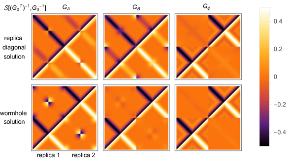
Figure 7: Contours and solutions for second-replicated action $\mathcal{S}[(G_{0}^{T})^{-1},G_{0}^{-1}]$. The arrows in the contours denote the time direction and the dashed lines denote the interactions. The parameters for the solutions are $J=K=1,\,V=0.5,\,q=4,\,p=2,\,s=r=1,\,N/M=0.1,\,N_{A}/N=0.75,\,\beta=0$, and $t=2$.

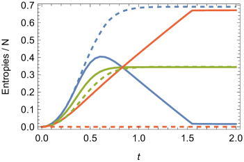
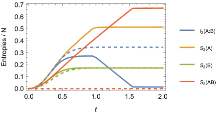
Figure 8: Renyi mutual information $I_{2}(A:B)$ and Renyi entropies $S_{2}(A),\ S_{2}(B),\ S_{2}(AB)$ in the SYK cluster coupled to bath. The parameters are $J=K=1$, (solid) $V=0.5$ or (dashed) $V=0$, $q=4,\,p=2,\,s=r=1,\,N/M=0.1,\,\beta=0$, and (left) $N_{A}/N=0.5$ or (right) $N_{A}/N=0.75$.

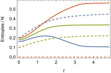
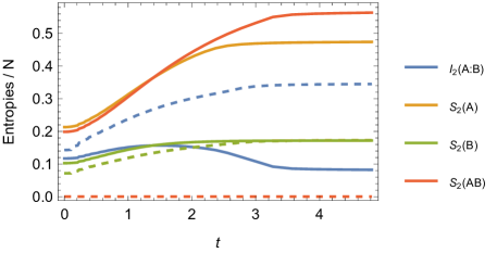
Figure 9: Renyi mutual information $I_{2}(A:B)$ and Renyi entropies $S_{2}(A),\ S_{2}(B),\ S_{2}(AB)$ in the SYK cluster coupled to bath. The parameters are the same as that in Fig. 9, except $\beta=2$.

We will numerically solve the SD equation for the $n=2$ replica. At the late time, there are two solutions in the replica action, including one replica diagonal solution and one wormhole solution, similar to Penington:2019kki . In Fig. 7, we show the contours and two solutions for action $\mathcal{S}[(G_{0}^{T})^{-1},G_{0}^{-1}]$ at the late time. From these two solutions, we should choose the one that results in a smaller value of the on-shell action. Finally, substituting the on-shell actions into (53) for different time $t$, we obtain the time evolution of Rényi entropy and Rényi mutual information, as shown in Figs. 8 and 9. We mainly focus on the case of $N_{B}\leq N_{A}\ll M$, $q=4,\,p=2,\,s=r=1$ and $V\lesssim J\sim K$. So the SYK cluster itself is chaotic and the bath itself is integrable. In general, the entropy and mutual information undergo through four stages:

1. All orders of Rényi entropy and the mutual information increase due to the interactions.

2. The entropy $S_{2}(B)$ is saturated. The growth of $S_{2}(A),S_{2}(AB)$ slightly slows down. The mutual information $I_{2}(A:B)$ stops growing.

3. The entropy $S_{2}(A)$ is saturated. The growth of $S_{2}(AB)$ slightly slows down. The mutual information $I_{2}(A:B)$ decays.

4. The entropy $S_{2}(AB)$ is saturated. The mutual information $I_{2}(A:B)$ reaches a plateau.

Notice that both the initial value and the final value of the mutual information $I_{2}(A:B)$ are zero for $\beta=0$ and finite for $\beta>0$. The evolution of the mutual information $I_{2}(A:B)$, indicates the entangling between $A$ and $B$ due to the $J$ interaction and disentangling due to the thermalization from the bath via the $V$ interaction.

To study the effect of baths on the internal entanglement of the SYK clusters, we compare the evolution of mutual information and entropies with and without the interaction between the SYK clusters and the baths in Figs. 8 and 9. As expected, $S_{2}(A:B)=0$ always and $S_{2}(A),\,S_{2}(B),\,I_{2}(A:B)$ grow and then become saturated. We can compare the case of $V\neq 0$ and $V=0$ to see the impact of baths.

When $\beta=0$, we observe that the entropies $S_{2}(A)$ and $S_{2}(B)$ in the $V\neq 0$ case grow faster than that in the $V=0$ case before their saturation. The enhancement of the growth rate is a natural consequence of the additional thermalization from baths. While the mutual information in the $V\neq 0$ case grows at the same rate as that in the $V=0$ case before the saturation of either $S_{2}(A)$ or $S_{2}(B)$. It implies that the thermalization due to the baths hardly affects the entanglement between $A$ and $B$ until one of their entropies becomes saturated.

When $\beta>0$, all the growth of $S_{2}(A),\,S_{2}(B),\,I_{2}(A:B)$ are affected by the bath. Their growth rates in the $V=0$ case are different from those in the $V\neq 0$ case. The reason is that the baths already affect the preparation of the initial state. In other words, the TFD state is given by the combined Hamiltonian (37) including the interaction term with the baths. It is different from the initial state at $\beta=0$, which is a maximally entangled state and is independent of the Hamiltonian.

4 Conclusion and outlook

In this paper, we have investigated the dynamic process of interior entanglement of two strongly coupled systems, including the gravity and SYK systems. The first model we have proposed is a doubly holographic model in $(3+1)$-dimensions, where the CFT matter sectors are dual to a $4$-dimensional bulk and the black hole is modeled by an EOW brane in the bulk. In the zero tension limit, the bulk geometry can be described by the standard SAdS metric with Neumann boundary conditions on the branes. By introducing a circular compactification in the $y$ direction, we have obtained a finite-sized black hole system from the boundary perspective. In this scenario, we have constructed the EWCS to quantify the reflected entropy between the black hole bipartition $\mathcal{BH}_{1}$ and $\mathcal{BH}_{2}$. Generally, the reflected entropy increases at early times due to the internal interactions of the black hole system. While at late times, these interior entanglements seep into the environment, since the interactions between the black hole system and the radiation drive the system to the final equilibrium. Moreover, we have extracted two universal patterns of evolution: For large black holes, a plateau emerges during the evolution of the reflected entropy, before the final equilibrium at a lower value. For moderate-sized black holes, no plateau emerges during the evolution, and the reflected entropy directly declines from the maximum to the final equilibrium value.

Our second model introduces a joint system comprising a SYK cluster, denoted as $\psi_{j}$, coupled to a large SYK bath, $\phi_{j}$. Specifically, the DOF in both SYK clusters and the bath are defined by the number of fermions they contain, expressed as $N=N_{A}+N_{B}$ and $M$, with $A$ and $B$ representing the bi-partition of the SYK clusters. In the large $N$ limit, this system is analyzed by numerically solving the SD equations. We have computed the second Rényi entropies and mutual information using the replica trick in this joint model. Our study covers different-sized bi-partitions of the SYK cluster, with $N_{A}\leq N_{B}$. Generally, we observe an initial increase in the mutual information of the bi-partition due to the internal interactions within the SYK cluster. At late times, the entanglement entropies of the subsystems saturate, while the entanglement between the SYK cluster and the bath continues to evolve. Consequently, the interior entanglement gradually leaks into the bath, eventually stabilizing at a relatively low equilibrium level.

For the first model, the zero tension condition is usually imposed in literature to circumvent the backreaction of the brane to the ambient geometry in the investigation of the dynamical evolution Ling:2020laa ; Liu:2022pan . Therefore, an intriguing area for future research lies in examining the dynamics within a backreacted spacetime. This challenge could potentially be addressed by employing the ingoing Eddington coordinates within the Einstein-DeTurck formulation Figueras:2012rb . It is important to note that in such a framework, the Einstein equations are transformed into a mixed elliptic-hyperbolic system, raising issues related to the local uniqueness of solutions Dias:2015nua . Aside from stationary scenarios, another promising avenue involves extending the numerical setup to non-equilibrium cases Janik:2017ykj ; Chen:2019uhq ; Chen:2022cwi ; Chen:2022tfy ; Zhang:2021etr ; Zhang:2022cmu ; Chen:2022vag ; Chen:2023eru , expanding the scope and applicability of the study to more dynamic and complex systems.

In both the gravity and SYK models, we have notice a pronounced difference between the evolution patterns of the reflected entropy and the mutual information. For any holographic state, there often exists a substantial gap of order $N^{2}$ between these two measures, known as the Markov gap Hayden:2021gno . This gap is commonly associated with the fidelity of a specific Markov recovery problem and has been a topic of extensive exploration in the context of double holography Lu:2022cgq ; Afrasiar:2022fid ; Afrasiar:2023jrj ; Basak:2023bnc . By comparing the plateau of the reflected entropy and the slope of the mutual information, we anticipate a noticeable enhancement of the Markov gap at late times but before the Page time. The reason for this enhancement deserves investigation in future studies.

Finally, in the model of SYK clusters coupled to baths, we can approximate the dynamics of the SYK clusters using the Lindblad master equation in the Born-Markov approximation Kawabata:2022osw ; Kulkarni:2021gtt ; Garcia-Garcia:2022adg . This approximation is expected to be valid under the conditions $N\ll M$ and $V\ll J\ll K$. The slope-stabilizing behavior observed in the mutual information here is akin to the slope-stabilizing behavior observed in the purity in the Lindbladian SYK Wang:2021woy , although in our case, the bipartite systems $A$ and $B$ are entangled due to their interactions during time evolution, rather than being initially configured to be in a TFD state. It would still be interesting to apply a large $q$ analysis as well as a quantum trajectories analysis in our model.

References

- (1) S.W. Hawking, Black hole explosions?, Nature 248 (1974) 30.
- (2) S.W. Hawking, Particle creation by black holes, in Euclidean quantum gravity, pp. 167–188, World Scientific (1975).
- (3) S.W. Hawking, Breakdown of predictability in gravitational collapse, Physical Review D 14 (1976) 2460.
- (4) L. Susskind, L. Thorlacius and J. Uglum, The stretched horizon and black hole complementarity, Physical Review D 48 (1993) 3743.
- (5) D. Harlow and P. Hayden, Quantum computation vs. firewalls, Journal of High Energy Physics 2013 (2013) 1.
- (6) A. Almheiri, D. Marolf, J. Polchinski and J. Sully, Black Holes: Complementarity or Firewalls?, JHEP 02 (2013) 062 [1207.3123].
- (7) J. Maldacena and L. Susskind, Cool horizons for entangled black holes, Fortsch. Phys. 61 (2013) 781 [1306.0533].
- (8) D.N. Page, Information in black hole radiation, Phys. Rev. Lett. 71 (1993) 3743 [hep-th/9306083].
- (9) D.N. Page, Hawking radiation and black hole thermodynamics, New J. Phys. 7 (2005) 203 [hep-th/0409024].
- (10) D.N. Page, Time Dependence of Hawking Radiation Entropy, JCAP 09 (2013) 028 [1301.4995].
- (11) G. Penington, Entanglement Wedge Reconstruction and the Information Paradox, 1905.08255.
- (12) A. Almheiri, N. Engelhardt, D. Marolf and H. Maxfield, The entropy of bulk quantum fields and the entanglement wedge of an evaporating black hole, JHEP 12 (2019) 063 [1905.08762].
- (13) A. Lewkowycz and J. Maldacena, Generalized gravitational entropy, JHEP 08 (2013) 090 [1304.4926].
- (14) N. Engelhardt and A.C. Wall, Quantum Extremal Surfaces: Holographic Entanglement Entropy beyond the Classical Regime, JHEP 01 (2015) 073 [1408.3203].
- (15) A. Almheiri, R. Mahajan, J. Maldacena and Y. Zhao, The Page curve of Hawking radiation from semiclassical geometry, JHEP 03 (2020) 149 [1908.10996].
- (16) A. Almheiri, T. Hartman, J. Maldacena, E. Shaghoulian and A. Tajdini, The entropy of Hawking radiation, Rev. Mod. Phys. 93 (2021) 035002 [2006.06872].
- (17) M. Alishahiha, A. Faraji Astaneh and A. Naseh, Island in the presence of higher derivative terms, JHEP 02 (2021) 035 [2005.08715].
- (18) K. Hashimoto, N. Iizuka and Y. Matsuo, Islands in Schwarzschild black holes, JHEP 06 (2020) 085 [2004.05863].
- (19) T. Anegawa and N. Iizuka, Notes on islands in asymptotically flat 2d dilaton black holes, JHEP 07 (2020) 036 [2004.01601].
- (20) T. Hartman, E. Shaghoulian and A. Strominger, Islands in Asymptotically Flat 2D Gravity, JHEP 07 (2020) 022 [2004.13857].
- (21) H.Z. Chen, Z. Fisher, J. Hernandez, R.C. Myers and S.-M. Ruan, Evaporating Black Holes Coupled to a Thermal Bath, JHEP 01 (2021) 065 [2007.11658].
- (22) A. Bhattacharya, A. Chanda, S. Maulik, C. Northe and S. Roy, Topological shadows and complexity of islands in multiboundary wormholes, JHEP 02 (2021) 152 [2010.04134].
- (23) F. Deng, J. Chu and Y. Zhou, Defect extremal surface as the holographic counterpart of Island formula, JHEP 03 (2021) 008 [2012.07612].
- (24) X. Wang, R. Li and J. Wang, Islands and Page curves of Reissner-Nordström black holes, JHEP 04 (2021) 103 [2101.06867].
- (25) S. He, Y. Sun, L. Zhao and Y.-X. Zhang, The universality of islands outside the horizon, JHEP 05 (2022) 047 [2110.07598].
- (26) F.F. Gautason, L. Schneiderbauer, W. Sybesma and L. Thorlacius, Page Curve for an Evaporating Black Hole, JHEP 05 (2020) 091 [2004.00598].
- (27) C. Krishnan, V. Patil and J. Pereira, Page Curve and the Information Paradox in Flat Space, 2005.02993.
- (28) W. Sybesma, Pure de Sitter space and the island moving back in time, Class. Quant. Grav. 38 (2021) 145012 [2008.07994].
- (29) C.-J. Chou, H.B. Lao and Y. Yang, Page curve of effective Hawking radiation, Phys. Rev. D 106 (2022) 066008 [2111.14551].
- (30) T.J. Hollowood, S.P. Kumar, A. Legramandi and N. Talwar, Grey-body factors, irreversibility and multiple island saddles, JHEP 03 (2022) 110 [2111.02248].
- (31) K. Suzuki and T. Takayanagi, BCFT and Islands in two dimensions, JHEP 06 (2022) 095 [2202.08462].
- (32) Y.-k. Suzuki and S. Terashima, On the dynamics in the AdS/BCFT correspondence, JHEP 09 (2022) 103 [2205.10600].
- (33) A. Bhattacharya, A. Bhattacharyya, P. Nandy and A.K. Patra, Bath deformations, islands, and holographic complexity, Phys. Rev. D 105 (2022) 066019 [2112.06967].
- (34) A. Bhattacharya, A. Bhattacharyya, P. Nandy and A.K. Patra, Partial islands and subregion complexity in geometric secret-sharing model, JHEP 12 (2021) 091 [2109.07842].
- (35) E. Caceres, A. Kundu, A.K. Patra and S. Shashi, Page curves and bath deformations, SciPost Phys. Core 5 (2022) 033 [2107.00022].
- (36) A. Bhattacharya, A. Bhattacharyya, P. Nandy and A.K. Patra, Islands and complexity of eternal black hole and radiation subsystems for a doubly holographic model, JHEP 05 (2021) 135 [2103.15852].
- (37) E. Caceres, A. Kundu, A.K. Patra and S. Shashi, Warped information and entanglement islands in AdS/WCFT, JHEP 07 (2021) 004 [2012.05425].
- (38) Y. Chen, Pulling Out the Island with Modular Flow, JHEP 03 (2020) 033 [1912.02210].
- (39) V. Balasubramanian, A. Kar, O. Parrikar, G. Sárosi and T. Ugajin, Geometric secret sharing in a model of Hawking radiation, JHEP 01 (2021) 177 [2003.05448].
- (40) L. Anderson, O. Parrikar and R.M. Soni, Islands with gravitating baths: towards ER = EPR, JHEP 21 (2020) 226 [2103.14746].
- (41) V. Balasubramanian, B. Craps, M. Khramtsov and E. Shaghoulian, Submerging islands through thermalization, JHEP 10 (2021) 048 [2107.14746].
- (42) N. Engelhardt and r. Folkestad, Canonical purification of evaporating black holes, Phys. Rev. D 105 (2022) 086010 [2201.08395].
- (43) C.-J. Chou, H.B. Lao and Y. Yang, Page Curve of AdS-Vaidya Model for Evaporating Black Holes, 2306.16744.
- (44) H.-S. Jeong, K.-Y. Kim and Y.-W. Sun, Entanglement entropy analysis of dyonic black holes using doubly holographic theory, Phys. Rev. D 108 (2023) 126016 [2305.18122].
- (45) B. Ahn, S.-E. Bak, H.-S. Jeong, K.-Y. Kim and Y.-W. Sun, Islands in charged linear dilaton black holes, Phys. Rev. D 105 (2022) 046012 [2107.07444].
- (46) A. Karch, H. Sun and C.F. Uhlemann, Double holography in string theory, JHEP 10 (2022) 012 [2206.11292].
- (47) C.F. Uhlemann, Islands and Page curves in 4d from Type IIB, JHEP 08 (2021) 104 [2105.00008].
- (48) A. Almheiri, R. Mahajan and J. Maldacena, Islands outside the horizon, arXiv:1910.11077 (2019) .
- (49) G. Penington, S.H. Shenker, D. Stanford and Z. Yang, Replica wormholes and the black hole interior, JHEP 03 (2022) 205 [1911.11977].
- (50) H.Z. Chen, Z. Fisher, J. Hernandez, R.C. Myers and S.-M. Ruan, Information Flow in Black Hole Evaporation, JHEP 03 (2020) 152 [1911.03402].
- (51) A. Almheiri, R. Mahajan and J.E. Santos, Entanglement islands in higher dimensions, SciPost Phys. 9 (2020) 001 [1911.09666].
- (52) T. Takayanagi, Holographic Dual of BCFT, Phys. Rev. Lett. 107 (2011) 101602 [1105.5165].
- (53) M. Nozaki, T. Takayanagi and T. Ugajin, Central Charges for BCFTs and Holography, JHEP 06 (2012) 066 [1205.1573].
- (54) K. Izumi, T. Shiromizu, K. Suzuki, T. Takayanagi and N. Tanahashi, Brane dynamics of holographic BCFTs, JHEP 10 (2022) 050 [2205.15500].
- (55) J. Erdmenger, M. Flory and M.-N. Newrzella, Bending branes for DCFT in two dimensions, JHEP 01 (2015) 058 [1410.7811].
- (56) J. Erdmenger, M. Flory, C. Hoyos, M.-N. Newrzella and J.M.S. Wu, Entanglement Entropy in a Holographic Kondo Model, Fortsch. Phys. 64 (2016) 109 [1511.03666].
- (57) C.-S. Chu and R.-X. Miao, Anomalous Transport in Holographic Boundary Conformal Field Theories, JHEP 07 (2018) 005 [1804.01648].
- (58) R.-X. Miao, Holographic BCFT with Dirichlet Boundary Condition, JHEP 02 (2019) 025 [1806.10777].
- (59) Y. Ling, Y. Liu and Z.-Y. Xian, Island in Charged Black Holes, JHEP 03 (2021) 251 [2010.00037].
- (60) H.Z. Chen, R.C. Myers, D. Neuenfeld, I.A. Reyes and J. Sandor, Quantum Extremal Islands Made Easy, Part I: Entanglement on the Brane, JHEP 10 (2020) 166 [2006.04851].
- (61) H. Geng, A. Karch, C. Perez-Pardavila, S. Raju, L. Randall, M. Riojas et al., Information Transfer with a Gravitating Bath, SciPost Phys. 10 (2021) 103 [2012.04671].
- (62) H. Geng and A. Karch, Massive islands, JHEP 09 (2020) 121 [2006.02438].
- (63) C. Krishnan, Critical Islands, JHEP 01 (2021) 179 [2007.06551].
- (64) H.Z. Chen, R.C. Myers, D. Neuenfeld, I.A. Reyes and J. Sandor, Quantum Extremal Islands Made Easy, Part II: Black Holes on the Brane, JHEP 12 (2020) 025 [2010.00018].
- (65) J. Hernandez, R.C. Myers and S.-M. Ruan, Quantum extremal islands made easy. Part III. Complexity on the brane, JHEP 02 (2021) 173 [2010.16398].
- (66) G. Grimaldi, J. Hernandez and R.C. Myers, Quantum extremal islands made easy. Part IV. Massive black holes on the brane, JHEP 03 (2022) 136 [2202.00679].
- (67) R.-X. Miao, An Exact Construction of Codimension two Holography, JHEP 01 (2021) 150 [2009.06263].
- (68) I. Akal, Y. Kusuki, T. Takayanagi and Z. Wei, Codimension two holography for wedges, Phys. Rev. D 102 (2020) 126007 [2007.06800].
- (69) I. Akal, Y. Kusuki, N. Shiba, T. Takayanagi and Z. Wei, Entanglement Entropy in a Holographic Moving Mirror and the Page Curve, Phys. Rev. Lett. 126 (2021) 061604 [2011.12005].
- (70) F. Omidi, Entropy of Hawking radiation for two-sided hyperscaling violating black branes, JHEP 04 (2022) 022 [2112.05890].
- (71) A. Almheiri, T. Hartman, J. Maldacena, E. Shaghoulian and A. Tajdini, Replica Wormholes and the Entropy of Hawking Radiation, JHEP 05 (2020) 013 [1911.12333].
- (72) M. Rozali, J. Sully, M. Van Raamsdonk, C. Waddell and D. Wakeham, Information radiation in BCFT models of black holes, JHEP 05 (2020) 004 [1910.12836].
- (73) A. Karlsson, Replica wormhole and island incompatibility with monogamy of entanglement, 2007.10523.
- (74) A. Kitaev, “A simple model of quantum holography.” http://online.kitp.ucsb.edu/online/entangled15/kitaev/ http://online.kitp.ucsb.edu/online/entangled15/kitaev2/, 2015.
- (75) J. Maldacena and D. Stanford, Remarks on the sachdev-ye-kitaev model, Phys. Rev. D 94 (2016) 106002 [1604.07818].
- (76) P. Zhang, Evaporation dynamics of the sachdev-ye-kitaev model, Phys. Rev. B 100 (2019) 245104.
- (77) A. Almheiri, A. Milekhin and B. Swingle, Universal Constraints on Energy Flow and SYK Thermalization, 1912.04912.
- (78) Y. Gu, X.-L. Qi and D. Stanford, Local criticality, diffusion and chaos in generalized Sachdev-Ye-Kitaev models, JHEP 05 (2017) 125 [1609.07832].
- (79) Y. Gu, A. Lucas and X.-L. Qi, Spread of entanglement in a Sachdev-Ye-Kitaev chain, JHEP 09 (2017) 120 [1708.00871].
- (80) S.-K. Jian and B. Swingle, Note on entropy dynamics in the Brownian SYK model, JHEP 03 (2021) 042 [2011.08158].
- (81) Y. Chen, X.-L. Qi and P. Zhang, Replica wormhole and information retrieval in the SYK model coupled to Majorana chains, JHEP 06 (2020) 121 [2003.13147].
- (82) Y. Liu, Z.-Y. Xian, C. Peng and Y. Ling, Black holes entangled by radiation, JHEP 09 (2022) 179 [2205.14596].
- (83) P.J. Dodd and J.J. Halliwell, Disentanglement and decoherence by open system dynamics, Phys. Rev. A 69 (2004) 052105.
- (84) Z. Sun, X. Wang and C.P. Sun, Disentanglement in a quantum-critical environment, Phys. Rev. A 75 (2007) 062312.
- (85) Y.-S. Kim, J.-C. Lee, O. Kwon and Y.-H. Kim, Protecting entanglement from decoherence using weak measurement and quantum measurement reversal, Nature Physics 8 (2012) 117.
- (86) M. Afrasiar, J. Kumar Basak, A. Chandra and G. Sengupta, Islands for Entanglement Negativity in Communicating Black Holes, arXiv:2205.07903 (2022) .
- (87) H. Geng, S. Lüst, R.K. Mishra and D. Wakeham, Holographic BCFTs and Communicating Black Holes, jhep 08 (2021) 003 [2104.07039].
- (88) H. Geng, A. Karch, C. Perez-Pardavila, S. Raju, L. Randall, M. Riojas et al., Entanglement phase structure of a holographic BCFT in a black hole background, JHEP 05 (2022) 153 [2112.09132].
- (89) H. Wang, C. Liu, P. Zhang and A.M. García-García, Entanglement Transition and Replica Wormhole in the Dissipative Sachdev-Ye-Kitaev Model, 2306.12571.
- (90) L. Randall and R. Sundrum, An Alternative to compactification, Phys. Rev. Lett. 83 (1999) 4690 [hep-th/9906064].
- (91) G. Dvali, G. Gabadadze and M. Porrati, 4-D gravity on a brane in 5-D Minkowski space, Phys. Lett. B 485 (2000) 208 [hep-th/0005016].
- (92) S.S. Gubser, AdS / CFT and gravity, Phys. Rev. D 63 (2001) 084017 [hep-th/9912001].
- (93) R.-X. Miao, C.-S. Chu and W.-Z. Guo, New proposal for a holographic boundary conformal field theory, Phys. Rev. D 96 (2017) 046005 [1701.04275].
- (94) C.-S. Chu, R.-X. Miao and W.-Z. Guo, On New Proposal for Holographic BCFT, JHEP 04 (2017) 089 [1701.07202].
- (95) G.W. Gibbons and S.W. Hawking, Action integrals and partition functions in quantum gravity, Phys. Rev. D 15 (1977) 2752.
- (96) M. Bianchi, D.Z. Freedman and K. Skenderis, Holographic renormalization, Nucl. Phys. B 631 (2002) 159 [hep-th/0112119].
- (97) H. Elvang and M. Hadjiantonis, A Practical Approach to the Hamilton-Jacobi Formulation of Holographic Renormalization, JHEP 06 (2016) 046 [1603.04485].
- (98) S. Dutta and T. Faulkner, A canonical purification for the entanglement wedge cross-section, JHEP 03 (2021) 178 [1905.00577].
- (99) Y. Ling, P. Liu, Y. Liu, C. Niu, Z.-Y. Xian and C.-Y. Zhang, Reflected entropy in double holography, JHEP 02 (2022) 037 [2109.09243].
- (100) Y. Liu, Q. Chen, Y. Ling, C. Peng, Y. Tian and Z.-Y. Xian, Entanglement of defect subregions in double holography, 2312.08025.
- (101) T. Hartman and J. Maldacena, Time Evolution of Entanglement Entropy from Black Hole Interiors, JHEP 05 (2013) 014 [1303.1080].
- (102) K. Su, P. Zhang and H. Zhai, Page curve from non-Markovianity, JHEP 21 (2020) 156 [2101.11238].
- (103) P. Figueras and T. Wiseman, Stationary holographic plasma quenches and numerical methods for non-Killing horizons, Phys. Rev. Lett. 110 (2013) 171602 [1212.4498].
- (104) O.J. Dias, J.E. Santos and B. Way, Numerical Methods for Finding Stationary Gravitational Solutions, Class. Quant. Grav. 33 (2016) 133001 [1510.02804].
- (105) R.A. Janik, J. Jankowski and H. Soltanpanahi, Real-Time dynamics and phase separation in a holographic first order phase transition, Phys. Rev. Lett. 119 (2017) 261601 [1704.05387].
- (106) Q. Chen, Y. Liu, Y. Tian, B. Wang, C.-Y. Zhang and H. Zhang, Critical dynamics in holographic first-order phase transition, JHEP 01 (2023) 056 [2209.12789].
- (107) Q. Chen, Y. Liu, Y. Tian, X. Wu and H. Zhang, Quench Dynamics in Holographic First-Order Phase Transition, 2211.11291.
- (108) C.-Y. Zhang, P. Liu, Y. Liu, C. Niu and B. Wang, Dynamical charged black hole spontaneous scalarization in anti–de Sitter spacetimes, Phys. Rev. D 104 (2021) 084089 [2103.13599].
- (109) C.-Y. Zhang, Q. Chen, Y. Liu, W.-K. Luo, Y. Tian and B. Wang, Dynamical transitions in scalarization and descalarization through black hole accretion, Phys. Rev. D 106 (2022) L061501 [2204.09260].
- (110) Q. Chen, Z. Ning, Y. Tian, B. Wang and C.-Y. Zhang, Descalarization by quenching charged hairy black hole in asymptotically AdS spacetime, JHEP 01 (2023) 062 [2210.14539].
- (111) Q. Chen, Z. Ning, Y. Tian, B. Wang and C.-Y. Zhang, Nonlinear dynamics of hot, cold and bald Einstein-Maxwell-scalar black holes in AdS spacetime, 2307.03060.
- (112) P. Hayden, O. Parrikar and J. Sorce, The Markov gap for geometric reflected entropy, JHEP 10 (2021) 047 [2107.00009].
- (113) Y. Lu and J. Lin, The Markov gap in the presence of islands, JHEP 03 (2023) 043 [2211.06886].
- (114) M. Afrasiar, J.K. Basak, A. Chandra and G. Sengupta, Reflected entropy for communicating black holes. Part I. Karch-Randall braneworlds, JHEP 02 (2023) 203 [2211.13246].
- (115) M. Afrasiar, J.K. Basak, A. Chandra and G. Sengupta, Reflected Entropy for Communicating Black Holes II: Planck Braneworlds, 2302.12810.
- (116) J.K. Basak, D. Basu, V. Malvimat, H. Parihar and G. Sengupta, Holographic Reflected Entropy and Islands in Interface CFTs, 2312.12512.
- (117) K. Kawabata, A. Kulkarni, J. Li, T. Numasawa and S. Ryu, Dynamical quantum phase transitions in Sachdev-Ye-Kitaev Lindbladians, Phys. Rev. B 108 (2023) 075110 [2210.04093].
- (118) A. Kulkarni, T. Numasawa and S. Ryu, Lindbladian dynamics of the Sachdev-Ye-Kitaev model, Phys. Rev. B 106 (2022) 075138 [2112.13489].
- (119) A.M. García-García, L. Sá, J.J.M. Verbaarschot and J.P. Zheng, Keldysh wormholes and anomalous relaxation in the dissipative Sachdev-Ye-Kitaev model, Phys. Rev. D 107 (2023) 106006 [2210.01695].