Neutral electronic excitations and derivative discontinuities: An extended $N$-centered ensemble density functional theory perspective

Abstract

This work merges two different types of many-electron ensembles, namely the Theophilou–Gross–Oliveira–Kohn ensembles of ground and neutrally-excited states, and the more recent $N$-centered ensembles of neutral and charged ground states. On that basis, an in-principle exact and general, so-called extended $N$-centered, ensemble density-functional theory of charged and neutral electronic excitations is derived. We revisit in this context the concept of density-functional derivative discontinuity for neutral excitations, without ever invoking nor using the asymptotic behavior of the ensemble electronic density. The present mathematical construction fully relies on the weight dependence of the ensemble Hartree-exchange-correlation density-functional energy, which makes the theory applicable to lattice models and opens new perspectives for the description of gaps in mesoscopic systems.

I Introduction

Kohn–Sham density-functional theory (KS-DFT) Kohn and Sham (1965) is prominently used nowadays to obtain approximate but reliable ground-state electronic energies around the equilibrium geometries of large systems with up to thousands of electrons. To go beyond ground-state properties, time-dependent extensions have been proposed, such as linear response time-dependent DFT (TD-DFT), where the first-order KS response function and the Hartree-exchange-correlation (Hxc) density-functional kernel allow for the extraction of excited-state energies Casida and Huix-Rotllant (2012), or real-time (or propagation) TD-DFT that relies on the numerical propagation of the electronic equations-of-motion and is not limited in principle to perturbations falling into the linear regime Runge and Gross (1984). Alternatively, and popularized in condensed matter physics, the more involved many-body perturbation theory Onida et al. (2002); Martin et al. (2016) within $GW$ Hedin (1965); Golze et al. (2019); Marie et al. (2023) together with the Bethe–Salpeter equation, which relies on the two-particle (frequency-dependent) Green’s function, can be used Strinati (1988); Sottile et al. (2007); Blase et al. (2020). All the aforementioned methods are computationally more demanding than KS-DFT. Even more problematic, linear response TD-DFT does not generally give an accurate description of charge transfer excitations Fuks and Maitra (2014), and multiple excitations are even absent from the spectra Maitra et al. (2004), when the popular semi-local adiabatic approximation is employed Casida and Huix-Rotllant (2012); Lacombe and Maitra (2023).

During the last decade, increasing attention has been paid to time-independent ensemble extensions of DFT (ensemble DFT) Pastorczak et al. (2013); Pastorczak and Pernal (2014); Franck and Fromager (2014); Yang et al. (2014); Pribram-Jones et al. (2014); Filatov (2015); Senjean et al. (2015); Deur et al. (2017); Yang et al. (2017); Gould and Pittalis (2017); Gould et al. (2018); Deur et al. (2018); Gould and Pittalis (2019); Fromager (2020); Gould et al. (2020); Gould (2020); Loos and Fromager (2020); Gould and Kronik (2021); Gould and Pittalis (2023); Gould et al. (2023, 2022, 2021); Cernatic et al. (2022), from which in-principle exact excitation energies can be inferred with the same computational cost as regular (ground-state) KS-DFT. Such an extension was originally proposed by Theophilou Theophilou (1979, 1987), Gross, Oliveira, and Kohn Gross et al. (1988a) for neutral excitation energies (i.e., difference of energy between states of a system with $N$ electrons) and is referred to as TGOK-DFT, following the name of the authors. The use of TGOK ensembles in other settings than DFT, both for the description of electronic and bosonic low-lying excited states, has also become increasingly appealing Schilling and Pittalis (2021); Liebert et al. (2022); Benavides-Riveros et al. (2022); Liebert and Schilling (2023a, b).

Quite recently, the concept of $N$-centered ensemble Senjean and Fromager (2018, 2020) has been introduced by analogy with TGOK-DFT to evaluate, in principle exactly, charged excitation energies (i.e., excitation energies between ground states corresponding to different electron numbers). Importantly, $N$-centered ensemble DFT shed a new light on the concept of density-functional derivative discontinuity for charged excitations, which emerged from the seminal work of Perdew, Parr, Levy, and Balduz (PPLB) in the context of DFT for fractional particle number Perdew et al. (1982); Perdew and Levy (1983). Within the formulation of PPLB, it is in principle sufficient to extend the domain of definition of the Hxc density functional to fractional electron numbers in order to account for derivative discontinuities. However, it has been argued that invoking a fractional number of electrons is maybe not the correct route to pursue Baerends et al. (2013); Baerends (2017, 2018, 2022, 2020). This debate aligns with the approach taken in $N$-centered ensemble DFT, where the derivative discontinuity is alternatively described through weight derivatives of the ensemble density-functional Hxc energy at fixed ensemble density. Such derivatives are well defined in the $N$-centered formalism since, by construction, the ensemble density always integrates to the fixed and central (integer) number of electrons $N$, hence the name of the theory. Extensive discussions about the equivalence between weight derivatives and derivative discontinuities for ground states can be found in Ref. Cernatic et al. (2022).

While a regular (so-called left in Ref. Senjean and Fromager, 2020) $N$-centered ensemble consists of $(N-1)$- and $N$-electron ground states, we propose in the present work to incorporate neutrally-excited (i.e., $N$-electron excited) states into the ensemble, thus allowing, for example, to decompose neutral excitation processes into separate ionization ones, as originally suggested by Levy Levy (1995). Even though we do not exploit in this work the following possibility, the formalism is flexible enough to include anionic states. The resulting hybrid TGOK/$N$-centered ensemble formalism, that we refer to as extended $N$-centered, lays the foundations of a unified and general ensemble density functional theory of charged and neutral electronic excitations. Most importantly, as shown in the following, this formalism sheds a different light on the concept of derivative discontinuity for neutral excitations Levy (1995); Yang et al. (2014); Gould et al. (2022), which is much less discussed in the literature than for charged excitations.

The paper is organized as follows. After motivating in Sec. II the decomposition of a neutral excitation process into two ionization processes, and reviewing briefly TGOK-DFT in Sec. III, we introduce the extended $N$-centered ensemble density-functional formalism in Sec. IV. On that basis, the concept of derivative discontinuity in the context of neutral excitation processes is revisited in Sec. V. The theory is then applied to the two-electron Hubbard dimer, as a proof of concept. The exact derivations and numerical tests are presented in Sec. VI. Conclusions and outlook are finally given in Sec. VII.

II Problematic: On the exactification of Kohn–Sham orbital energies

The occupied and virtual orbital energies $\left\{\varepsilon_{i}\right\}_{i=1,2,\ldots}$ generated from a regular $N$-electron ground-state KS-DFT calculation can be used to compute total ground- and excited-state $N$-electron KS energies,

$$\mathcal{E}^{N}_{\nu}=\sum_{i}n_{\nu}^{i}\varepsilon_{i},$$ (1)

where $n_{\nu}^{i}\in\left\{0,1,2\right\}$ denotes the integer occupation of the $i$th KS orbital in the $\nu$th KS state ($\nu\geq 0$) and $\sum_{i}n^{i}_{\nu}=N$. It is well-known that when it comes to describing neutral excitation processes, the bare KS excitation energies and the true interacting ones $\left\{\omega_{\nu}\right\}_{\nu>0}$ do not match:

$$\omega_{\nu}\equiv E^{N}_{\nu}-E^{N}_{0}\neq\mathcal{E}^{N}_{\nu}-\mathcal{E}^{N}_{0}.$$ (2)

In the context of linear response TD-DFT, these two quantities are connected through the Hxc kernel, i.e., the density-functional derivative of the (time-dependent) Hxc potential. We focus in the following on in-principle-exact time-independent density-functional approaches to neutral electronic excitations and, more specifically, to ensemble ones. At this point we should stress that, unlike in charged processes, any constant shift in the Hxc potential and therefore in the orbital energies,

$$\varepsilon_{i}\rightarrow\varepsilon_{i}+c,$$ (3)

leaves neutral KS excitation energies unchanged:

$$\mathcal{E}_{\nu}^{N}-\mathcal{E}^{N}_{0}\rightarrow\left(\mathcal{E}^{N}_{\nu}+Nc\right)-\left(\mathcal{E}^{N}_{0}+Nc\right)=\mathcal{E}^{N}_{\nu}-\mathcal{E}^{N}_{0}.$$ (4)

From this standpoint, it seems impossible to exactify the KS orbital energies in the description of neutrally excited states. Nevertheless, as recalled in Sec. III, it is possible to describe exactly the deviation of the physical excitation energy from the KS one by means of an ensemble-weight-dependent Hxc density functional.

In the present work, we follow a connected but slightly different path by achieving such a description through an exactification of the KS orbital energies for specific excitations. Based on the observation made in Eq. (4) and the seminal work of Levy Levy (1995), the key idea consists in evaluating a neutral excitation energy via two different charged processes, namely the ionization of the ground ($\nu=0$) and the targeted excited ($\nu>0$) $N$-electron states, i.e.,

$$E^{N}_{\nu}-E^{N}_{0}=I^{N}_{0}-I^{N}_{\nu},$$ (5)

where

$$\left\{I^{N}_{\nu}=E^{N-1}_{0}-E^{N}_{\nu}\right\}_{\nu\geq 0}$$ (6)

will be referred to as ground- and excited-state ionization potentials (IPs).

Turning to the KS system, for each ionization process, a specific shift can be applied to the Hxc potential (which is unique up to a constant, as long as the number of electrons is fixed to the integer $N$) in order to enforce the KS IPs to match the true interacting ones, i.e.,

$$\begin{split}\varepsilon_{i}&\rightarrow\varepsilon_{i}+c_{1}=\overline{\varepsilon}_{i},\\ \mathcal{E}^{N-1}_{0}-\mathcal{E}^{N}_{0}&\rightarrow\mathcal{E}^{N-1}_{0}-\mathcal{E}^{N}_{0}-c_{1}\overset{!}{=}I^{N}_{0},\end{split}$$ (7)

and

$$\begin{split}\varepsilon_{i}&\rightarrow\varepsilon_{i}+c_{2}=\tilde{\varepsilon}_{i},\\ \mathcal{E}^{N-1}_{0}-\mathcal{E}^{N}_{\nu}&\rightarrow\mathcal{E}^{N-1}_{0}-\mathcal{E}^{N}_{\nu}-c_{2}\overset{!}{=}I^{N}_{\nu}.\end{split}$$ (8)

If, for example, the excited state of interest $\nu$ is described by a single-electron excitation (one hole, one particle) from the highest occupied molecular orbital (HOMO) $i=N$ to a virtual one $i=N+\nu$, then we automatically obtain from Eqs. (5), (7), and (8) what we consider as the exactification of the KS orbital energies for neutral excitations, i.e.,

$$E^{N}_{\nu}-E^{N}_{0}=\tilde{\varepsilon}_{N+\nu}-\overline{\varepsilon}_{N}.$$ (9)

The question that is addressed in the rest of this work is how such a construction can be derived, in principle exactly, from a unified and general ensemble density-functional formalism in which both charged and neutral excitation processes can be described simultaneously.

III Brief review of regular TGOK ensemble DFT

TGOK-DFT is a time-independent ensemble extension of standard ground-state DFT to neutral excited states where the ground-state energy is replaced by the so-called ensemble energy, which is a convex combination of ($N$-electron) ground- and excited-state energies,

$$E^{\bm{\xi}}\overset{\rm TGOK}{:=}\left(1-\sum_{\nu>0}\xi^{N}_{\nu}\right)E_{0}^{N}+\sum_{\nu>0}\xi^{N}_{\nu}E^{N}_{\nu},$$ (10)

where

$$\bm{\xi}\overset{\rm TGOK}{\equiv}\left\{\xi^{N}_{\nu}\right\}_{\nu>0}$$ (11)

is the collection of positive and independent ensemble weight values that are assigned to the ordered-in-energy $N$-electron excited states $\left\{\Psi_{\nu}^{N}\right\}_{\nu>0}$, i.e.,

$$E_{\nu}^{N}=\matrixelement{\Psi_{\nu}^{N}}{\hat{H}}{\Psi_{\nu}^{N}}<E_{\nu+1}^{N}.$$ (12)

The electronic Hamiltonian operator $\hat{H}$ of the system under study reads

$$\hat{H}=\hat{T}+\hat{W}_{\rm ee}+\hat{V}_{\rm ext},$$ (13)

where $\hat{T}$ describes the kinetic energy, $\hat{W}_{\rm ee}$ is the two-electron repulsion operator, $\hat{V}_{\rm ext}=\int d\mathbf{r}\,v_{\rm ext}(\mathbf{r})\hat{n}(\mathbf{r})$ is the external local potential operator, and $\hat{n}(\mathbf{r})$ denotes the density operator at position $\mathbf{r}$. Note that the weight $\xi_{0}^{N}$ assigned to the ground-state energy $E_{0}^{N}$ in Eq. (10) is such that the collection of weights (including the ground-state one) is normalized:

$$\xi_{0}^{N}+\sum_{\nu>0}\xi^{N}_{\nu}\overset{\rm{TGOK}}{=}1.$$ (14)

This constraint, where $\xi_{0}^{N}$ is an affine function of the independent excited-state ensemble weights Deur and Fromager (2019), ensures that the total number of electrons is preserved when deviating from the ground-state $\bm{\xi}=0$ limit of the theory, i.e.,

$$\int d\mathbf{r}\,n^{\bm{\xi}}(\mathbf{r})=N,\quad\forall\bm{\xi},$$ (15)

where

$$n^{\bm{\xi}}(\mathbf{r})\overset{\rm TGOK}{:=}\left(1-\sum_{\nu>0}\xi^{N}_{\nu}\right)n_{\Psi_{0}^{N}}({\mathbf{r}})+\sum_{\nu>0}\xi^{N}_{\nu}n_{\Psi_{\nu}^{N}}({\mathbf{r}})$$ (16)

is the ensemble density, $\left\{n_{\Psi_{\nu}^{N}}({\mathbf{r}})\right\}_{\nu\geq 0}$ being the individual $N$-electron ground- and excited-state densities. In the following, we use the more compact notation,

$$n^{\bm{\xi}}(\mathbf{r})=\Tr[\hat{\Gamma}^{\bm{\xi}}\hat{n}(\mathbf{r})],$$ (17)

where

$$\hat{\Gamma}^{\bm{\xi}}\overset{\rm TGOK}{=}\quantity(1-\sum_{\nu>0}\xi_{\nu}^{N})\outerproduct*{{\Psi}_{0}^{N}}{{\Psi}_{0}^{N}}+\sum_{\nu>0}\xi_{\nu}^{N}\outerproduct*{{\Psi}^{N}_{\nu}}{{\Psi}^{N}_{\nu}}$$ (18)

is the ensemble density matrix operator and $\Tr$ denotes the trace. Note that we have assumed, for simplicity, that both ground and excited states are not degenerate but the formalism can be extended straightforwardly to ensembles of multiplets Gross et al. (1988a).

The TGOK ensemble energy, as defined in Eqs. (10) and (12), can be determined variationally, i.e.,

$$E^{\bm{\xi}}=\min_{\hat{\gamma}^{\bm{\xi}}}\Tr[\hat{\gamma}^{\bm{\xi}}\hat{H}]=\Tr\left[\hat{\Gamma}^{\bm{\xi}}\hat{H}\right],$$ (19)

where $\hat{\gamma}^{\bm{\xi}}$ is a trial ensemble density matrix operator, provided that the ensemble weights are collected in decreasing order Gross et al. (1988b):

$$\xi^{N}_{\nu}\geq\xi^{N}_{\nu+1},\quad\nu\geq 0.$$ (20)

On that basis, an ensemble KS-DFT of neutral excited states can be derived Gross et al. (1988a), where the ensemble Hxc density functional is defined exactly, as follows

$$\begin{split}E_{\rm Hxc}^{\bm{\xi}}[n]&=\min_{\hat{\gamma}^{\bm{\xi}}\rightarrow n}\Tr[\hat{\gamma}^{\bm{\xi}}\left(\hat{T}+\hat{W}_{\rm ee}\right)]-\min_{\hat{\gamma}^{\bm{\xi}}\rightarrow n}\Tr[\hat{\gamma}^{\bm{\xi}}\hat{T}]\\ &:=F^{\bm{\xi}}[n]-T^{\bm{\xi}}_{\rm s}[n],\end{split}$$ (21)

where $F^{\bm{\xi}}[n]$ (and its noninteracting analogue $T^{\bm{\xi}}_{\rm s}[n]$) is simply the extension to ensembles (with given fixed ensemble weight values $\bm{\xi}$) of the Levy–Lieb functional Levy (1979); Lieb (1983). The density constraint used in both minimizations reads $n_{\hat{\gamma}^{\bm{\xi}}}(\mathbf{r})=\Tr[\hat{\gamma}^{\bm{\xi}}\hat{n}(\mathbf{r})]=n(\mathbf{r})$.

Note that the ensemble Hxc functional is both a functional of the density $n$ and a function of the ensemble weights $\bm{\xi}$. The reason is that, unlike in ground-state DFT of open electronic systems, where the ensemble weight is deduced from the fractional number of electrons, a TGOK ensemble cannot be identified solely from its density. Indeed, a density $n$ that integrates to a given integer number $N$ of electrons may be both pure-ground-state and ensemble $v$-representable at the same time [see Eq. (37) in Ref. Teale et al., 2022 and the discussion that follows]. Without additional information about the ensemble (namely the ensemble weight values), the functional would not “know” if it has to compute the Hxc energy of a pure ground state ($\bm{\xi}=0$) or that of an ensemble ($\bm{\xi}>0$).

Finally, like in ground-state KS-DFT, the ensemble density-functional Hxc energy can be decomposed into (weight-dependent) Hx and correlation contributions, which respectively read

$$E_{\rm Hx}^{\bm{\xi}}[n] =\Tr[\hat{\gamma}_{\rm KS}^{\bm{\xi}}[n]\hat{W}_{\rm ee}],$$ (22a)

$$E_{\rm c}^{\bm{\xi}}[n] =E_{\rm Hxc}^{\bm{\xi}}[n]-E_{\rm Hx}^{\bm{\xi}}[n],$$ (22b)

where $\hat{\gamma}_{\rm KS}^{\bm{\xi}}[n]=\operatorname*{arg\,min}_{\hat{\gamma}^{\bm{\xi}}\rightarrow n}\Tr[\hat{\gamma}^{\bm{\xi}}\hat{T}]$ is the density-functional noninteracting KS ensemble density matrix operator. Note that the separation into Hartree and exchange contributions of the ensemble Hx functional is not trivial nor unique Gidopoulos et al. (2002); Pastorczak and Pernal (2014); Gould et al. (2020); Gould and Kronik (2021); Cernatic et al. (2022), unlike in regular ground-state DFT. This point will be discussed a bit further after Eq. (58).

In the context of TGOK-DFT, the variational ensemble energy expression of Eq. (19) can be recast into a minimization over noninteracting ensemble density matrix operators

$$E^{\bm{\xi}}=\min_{\hat{\gamma}^{\bm{\xi}}}\left\{\Tr[\hat{\gamma}^{\bm{\xi}}\left(\hat{T}+\hat{V}_{\rm ext}\right)]+E_{\rm Hxc}^{\bm{\xi}}[n_{\hat{\gamma}^{\bm{\xi}}}]\right\},$$ (23)

where the (weight-dependent Cernatic et al. (2022)) minimizing KS wave functions $\left\{\Phi^{\bm{\xi}}_{\nu}\right\}_{\nu\geq 0}$ fulfill the following self-consistent noninteracting Schrödinger equation

$$\left[\hat{T}+\hat{V}_{\rm ext}+\int d\mathbf{r}\,v^{\bm{\xi}}_{\rm Hxc}(\mathbf{r})\hat{n}(\mathbf{r})\right]\ket{\Phi^{\bm{\xi}}_{\nu}}=\mathcal{E}^{\bm{\xi}}_{\nu}\ket{\Phi^{\bm{\xi}}_{\nu}},$$ (24)

$v^{\bm{\xi}}_{\rm Hxc}(\mathbf{r})=\left.\delta E_{\rm Hxc}^{\bm{\xi}}[n]/\delta n(\mathbf{r})\right|_{n=n^{\bm{\xi}}}$ being the weight-dependent Hxc potential. Equivalently, the orbitals from which the KS ensemble is constructed fulfill the following ensemble KS equations

$$\left[-\dfrac{\nabla_{\mathbf{r}}^{2}}{2}+v_{\rm ext}(\mathbf{r})+v^{\bm{\xi}}_{\rm Hxc}(\mathbf{r})\right]\varphi^{\bm{\xi}}_{i}(\mathbf{r})=\varepsilon^{\bm{\xi}}_{i}\varphi^{\bm{\xi}}_{i}(\mathbf{r}).$$ (25)

The latter differ from regular (ground-state) KS equations by i) the weight dependence of the Hxc potential, and ii) the fact that the KS orbitals, which reproduce the exact ensemble density $n^{\bm{\xi}}(\mathbf{r})$, are fractionally occupied, i.e.,

$$n^{\bm{\xi}}(\mathbf{r})=\sum_{\nu\geq 0}\xi_{\nu}n_{\Phi^{\bm{\xi}}_{\nu}}(\mathbf{r})=\sum_{i}\left(\sum_{\nu\geq 0}\xi_{\nu}n^{i}_{\nu}\right)\absolutevalue{\varphi^{\bm{\xi}}_{i}(\mathbf{r})}^{2},$$ (26)

where $n_{\nu}^{i}$ is the occupation of the KS orbital $\varphi^{\bm{\xi}}_{i}$ in the KS analog $\Phi^{\bm{\xi}}_{\nu}$ of the pure state $\nu$. Note that the (weight-dependent) total KS energies simply read

$$\mathcal{E}^{\bm{\xi}}_{\nu}=\sum_{i}n_{\nu}^{i}\varepsilon^{\bm{\xi}}_{i}.$$ (27)

Turning to the problematic raised in Sec. II, we should first recall that the exact deviation of the true interacting excitation energies from the KS ones is given by the derivative with respect to the ensemble weights (at fixed ensemble density) of the ensemble Hxc density-functional energy Gross et al. (1988a); Deur and Fromager (2019):

$$E^{N}_{\nu}-E^{N}_{0}-\left(\mathcal{E}^{\bm{\xi}}_{\nu}-\mathcal{E}^{\bm{\xi}}_{0}\right)=\left.\dfrac{\partial E_{\rm Hxc}^{\bm{\xi}}[n]}{\partial\xi^{N}_{\nu}}\right|_{n=n^{\bm{\xi}}}.$$ (28)

Therefore, within regular TGOK-DFT, the exactification of the ensemble KS orbital energies occurs only when the above ensemble weight derivative vanishes, which may happen for very specific (a priori unknown) weight values Yang et al. (2014); Deur et al. (2017). In other words, such an exactification cannot, in general, be achieved, unless we introduce intermediate ionization processes, as suggested in Sec. II. The main challenge in this case lies in the design of a unified ensemble density-functional formalism where both neutral and charged excitations can be described. A solution to this problem is proposed in Sec. IV.

IV Extended $N$-centered ensemble DFT

Senjean and Fromager Senjean and Fromager (2018) introduced some years ago the so-called $N$-centered ensemble DFT formalism where the fundamental gap of $N$-electron ground states is described with the exact same mathematical language as in TGOK-DFT. The approach also allows for a separate description of ionization and affinity processes Senjean and Fromager (2018, 2020); Hodgson et al. (2021); Cernatic et al. (2022), which is essential in the present context. The close resemblance of $N$-centered ensemble DFT with TGOK-DFT is exploited in the following in order to provide an in-principle exact ensemble density-functional description of ionized excited states. The resulting ensemble formalism, where neutral excited states are incorporated into a regular (ground-state) $N$-centered ensemble, will be referred to as extended $N$-centered ensemble formalism.

IV.1 Combining TGOK with $N$-centered ensembles

By analogy with regular $N$-centered ensemble DFT, where the ensemble weights assigned to the $(N-1)$- and $(N+1)$-electron ground states are allowed to vary independently Senjean and Fromager (2018), we propose to combine TGOK and $N$-centered ($N$c) ensembles as follows,

$$\hat{\Gamma}^{\bm{\xi}}\overset{{\rm TGOK}+N{\rm c}}{=}\quantity(1-\sum_{\nu>0}\dfrac{N_{\nu}}{N}\xi_{\nu})\outerproduct*{{\Psi}_{0}}{{\Psi}_{0}}+\sum_{\nu>0}\xi_{\nu}\outerproduct*{{\Psi}_{\nu}}{{\Psi}_{\nu}},$$ (29)

where $\Psi_{0}\equiv{\Psi}_{0}^{N}$ is the reference $N$-electron ground state to which all possible excitation processes (neutral and charged, including multiple-electron excitations) can be applied. In other words, the integer number of electrons $N_{\nu}=\int d\mathbf{r}\,n_{\Psi_{\nu}}(\mathbf{r})$ that is described by the excited-state wave function $\Psi_{\nu}$ ($\nu>0$) is not necessarily equal to the (integer) number of electrons in the ground state,

$$N_{0}=N,$$ (30)

that is referred to as the central number of electrons. However, by construction, the ensemble density still integrates to $N$, like in TGOK-DFT [see Eqs. (15) and (17)].

As further discussed in Sec. V, the fact that the net number of electrons in the ensemble does not vary with the ensemble weights, unlike in the traditional PPLB-DFT of fractional electron numbers Perdew et al. (1982), plays a central role in the exact description of derivative discontinuities in terms of ensemble weight derivatives Hodgson et al. (2021); Cernatic et al. (2022). More precisely, the key feature of $N$-centered ensemble DFT is the fact that ensemble weights can vary while holding the ensemble density fixed Senjean and Fromager (2018). In PPLB-DFT, the Hxc functional has no weight dependence (i.e., it is solely a functional of the density) simply because the ensemble weight is itself a functional of the density Cernatic et al. (2022) which can be defined, for example, as the deviation of the (fractional) electron number from its floor value. Hence, in PPLB-DFT, any variation in weight automatically induces a change in density.

Turning back to the extended $N$-centered ensemble of Eq. (29), we point out that the ensemble weights assigned to the ground and excited states are positive,

$$\xi_{0} =1-\sum_{\nu>0}\dfrac{N_{\nu}}{N}\xi_{\nu}\geq 0,$$ (31a)

$$\xi_{\nu} \geq 0,\quad\forall\nu>0,$$ (31b)

and, most importantly, unlike in conventional TGOK or PPLB ensembles, they do not sum up to 1, in general:

$$\sum_{\nu\geq 0}\xi_{\nu}=1+\sum_{\nu>0}\dfrac{\left(N-N_{\nu}\right)}{N}\xi_{\nu}.$$ (32)

In addition, within each subensemble containing all the states with the same number $N\pm p$ ($p=0,1,2,\ldots,N$) of electrons, we impose the following weight ordering constraints [see Eq. (20)],

$$\xi_{\nu}\overset{N_{\nu}=N_{\nu+1}=N\pm p}{\geq}\xi_{\nu+1},$$ (33)

in order to be able to exploit, if necessary, the TGOK variational principle within each $(N\pm p)$-electron sector of the Fock space. This simply ensures that the fully extended $N$-centered ensemble of interest can be determined variationally, thus allowing for an in-principle-exact density-functional description of its energy. Note that, in the present work, the constraint of Eq. (33) will be used only for $N$-electron states (i.e., $p=0$) while the $(N-1)$ sector will be reduced to ground states. The $(N+1)$ sector will not be used. These choices are motivated by the problem raised in Sec. II and are by no means a limitation of the present ensemble formalism, which is very general.

Let us finally turn to the extended $N$-centered ensemble energy,

$$E^{\bm{\xi}}\overset{{\rm TGOK}+N{\rm c}}{=}\quantity(1-\sum_{\nu>0}\dfrac{N_{\nu}}{N}\xi_{\nu})E_{0}+\sum_{\nu>0}\xi_{\nu}E_{\nu},$$ (34)

where $E_{0}=E_{0}^{N}$ is the reference $N$-electron ground-state energy and $E_{\nu}$ is an $N_{\nu}$-electron eigenvalue of the electronic Hamiltonian, i.e.,

$$\hat{H}\ket{\Psi_{\nu}}=E_{\nu}\ket{\Psi_{\nu}},\quad\nu\geq 0,$$ (35)

with $N_{\nu}\in\left\{N,N\pm 1,N\pm 2,\ldots\right\}$. Like in TGOK-DFT Deur and Fromager (2019), the linearity of the ensemble energy in the ensemble weights,

$$\bm{\xi}\overset{{\rm TGOK}+N{\rm c}}{\equiv}\left\{\xi_{\nu}\right\}_{\nu>0},$$ (36)

allows for a straightforward extraction of individual energy levels (and, therefore, of the excitation energies) through first-order differentiations. Indeed, since both ground-state ($\nu=0$) [see Eq. (30)] and excited-state ($\nu>0$) energies can be expressed as follows,

$$E_{\nu}\underset{\nu\geq 0}{=}\dfrac{N_{\nu}}{N}E_{0}+\sum_{\lambda>0}\delta_{\lambda\nu}\left(E_{\lambda}-\dfrac{N_{\lambda}}{N}E_{0}\right),$$ (37)

where, according to Eq. (34),

$$\dfrac{\partial E^{\bm{\xi}}}{\partial\xi_{\lambda}}=E_{\lambda}-\dfrac{N_{\lambda}}{N}E_{0},$$ (38)

and

$$E_{0}=E^{\bm{\xi}}-\sum_{\lambda>0}\xi_{\lambda}\dfrac{\partial E^{\bm{\xi}}}{\partial\xi_{\lambda}},$$ (39)

we immediately obtain the following compact expression in terms of the ensemble energy (and its first-order derivatives),

$$E_{\nu}\underset{\nu\geq 0}{=}\dfrac{N_{\nu}}{N}E^{\bm{\xi}}+\sum_{\lambda>0}\quantity(\delta_{\lambda\nu}-\dfrac{N_{\nu}}{N}\xi_{\lambda})\dfrac{\partial E^{\bm{\xi}}}{\partial\xi_{\lambda}}.$$ (40)

Note that Eq. (40) generalizes expressions that have been derived previously and separately in regular TGOK Deur and Fromager (2019) (for neutral excited states) and $N$-centered Senjean and Fromager (2018); Cernatic et al. (2022) (for charged excited states) ensemble theories. As shown in the following section, once a KS density-functional description of the extended $N$-centered ensemble energy $E^{\bm{\xi}}$ is established, it becomes possible to relate formally any charged or neutral KS excitation energy to the true physical one.

IV.2 Density-functionalization of the approach

According to both regular (ground-state) Rayleigh–Ritz and TGOK Theophilou (1979); Gross et al. (1988b) variational principles, the extended $N$-centered ensemble energy of Eq. (34) can be determined variationally, thus allowing for its in-principle-exact ensemble density-functional description. The exact same formalism as in TGOK-DFT can actually be used [see Eqs. (23)–(27)]. The only difference is that we are now allowed to consider occupations in the KS wave functions [see Eq. (27)] that do not necessarily sum up to $N$:

$$\sum_{i}n_{\nu}^{i}=N_{\nu}.$$ (41)

By rewriting the ensemble energy as follows [see Eqs. (23), (24), and (26)]

$$E^{\bm{\xi}}=\sum_{\nu\geq 0}\xi_{\nu}\mathcal{E}^{\bm{\xi}}_{\nu}+E_{\rm Hxc}^{\bm{\xi}}[n^{\bm{\xi}}]-\int d\mathbf{r}\,v_{\rm Hxc}^{\bm{\xi}}(\mathbf{r})n^{\bm{\xi}}(\mathbf{r}),$$ (42)

and applying the Hellmann-Feynman theorem to its variational expression in Eq. (23), which leads to

$$\dfrac{\partial E^{\bm{\xi}}}{\partial\xi_{\lambda}}=\mathcal{E}^{\bm{\xi}}_{\lambda}-\dfrac{N_{\lambda}}{N}\mathcal{E}^{\bm{\xi}}_{0}+\left.\dfrac{\partial E_{\rm Hxc}^{\bm{\xi}}[n]}{\partial\xi_{\lambda}}\right|_{n=n^{\bm{\xi}}},$$ (43)

we deduce from Eq. (40) the following exact expression for any individual energy level included into the ensemble

$$\begin{split}E_{\nu}\underset{\nu\geq 0}{=}\mathcal{E}^{\bm{\xi}}_{\nu}&+\dfrac{N_{\nu}}{N}\left(E_{\rm Hxc}^{\bm{\xi}}[n^{\bm{\xi}}]-\int d\mathbf{r}\,v_{\rm Hxc}^{\bm{\xi}}(\mathbf{r})n^{\bm{\xi}}(\mathbf{r})\right)\\ &+\sum_{\lambda>0}\quantity(\delta_{\lambda\nu}-\dfrac{N_{\nu}}{N}\xi_{\lambda})\left.\dfrac{\partial E_{\rm Hxc}^{\bm{\xi}}[n]}{\partial\xi_{\lambda}}\right|_{n=n^{\bm{\xi}}},\end{split}$$ (44)

where, in the second term on the right-hand side, we recognize the analog for ensembles of the Levy–Zahariev shift in potential Levy and Zahariev (2014); Deur and Fromager (2019); Senjean and Fromager (2018). At this point we should make an important observation that will be exploited later on, namely that the above expression is invariant under constant shifts in the ensemble Hxc potential, $v_{\rm Hxc}^{\bm{\xi}}(\mathbf{r})\rightarrow v_{\rm Hxc}^{\bm{\xi}}(\mathbf{r})+c$, since [see Eqs. (15), (27), and (41)]

$$\mathcal{E}^{\bm{\xi}}_{\nu}-\dfrac{N_{\nu}}{N}\int d\mathbf{r}\,v_{\rm Hxc}^{\bm{\xi}}(\mathbf{r})n^{\bm{\xi}}(\mathbf{r})\\ =\left(\mathcal{E}^{\bm{\xi}}_{\nu}+N_{\nu}c\right)-\dfrac{N_{\nu}}{N}\int d\mathbf{r}\,\left(v_{\rm Hxc}^{\bm{\xi}}(\mathbf{r})+c\right)n^{\bm{\xi}}(\mathbf{r}),$$ (45)

even though the ensemble may contain states that describe different numbers of electrons. This major difference between (extended or not) $N$-centered ensemble DFT and the conventional DFT for fractional electron numbers originates from the fact that, in the former theory, the number of electrons is artificially held constant and equal to the integer $N$ [see Eq. (15)].

We finally conclude from Eq. (44) that the energy associated to any (charged or neutral) excitation $\nu\rightarrow\kappa$ can be expressed exactly in terms of its KS analog as follows

$$\begin{split}&E_{\kappa}-E_{\nu}=\mathcal{E}^{\bm{\xi}}_{\kappa}-\mathcal{E}^{\bm{\xi}}_{\nu}\\ &+\dfrac{\left(N_{\kappa}-N_{\nu}\right)}{N}\left(E_{\rm Hxc}^{\bm{\xi}}[n^{\bm{\xi}}]-\int d\mathbf{r}\,v_{\rm Hxc}^{\bm{\xi}}(\mathbf{r})n^{\bm{\xi}}(\mathbf{r})\right)\\ &+\sum_{\lambda>0}\quantity(\delta_{\lambda\kappa}-\delta_{\lambda\nu}-\dfrac{\left(N_{\kappa}-N_{\nu}\right)}{N}\xi_{\lambda})\left.\dfrac{\partial E_{\rm Hxc}^{\bm{\xi}}[n]}{\partial\xi_{\lambda}}\right|_{n=n^{\bm{\xi}}}.\end{split}$$ (46)

Equation (46) is our first key result. It generalizes the neutral excitation energy expression of TGOK-DFT Gross et al. (1988a); Deur and Fromager (2019) that was recalled in Eq. (28).

V Revisiting density-functional derivative discontinuities induced by neutral excitations

In order to achieve an exactification of the KS orbital energies along the lines of Sec. II, we apply the general formalism of Sec. IV to a particular type of extended $N$-centered ensemble which includes only the neutrally-excited $N$-electron states, with weights $\left\{\xi_{\lambda}^{N}\right\}_{\lambda>0}$, and the ionized $(N-1)$-electron ground state, with weight $\xi_{-}:=\xi^{N-1}_{0}$. Therefore, in this special case, the collection of ensemble weights reduces to

$$\bm{\xi}\equiv\left(\left\{\xi^{N}_{\lambda}\right\}_{\lambda>0},\xi_{-}\right).$$ (47)

According to Eqs. (6) and (46), where $\kappa$ now refers to the ionized ground state and $\nu$ to the ground or excited $N$-electron state of interest, the exact ground- and excited-state IPs read

$$\begin{split}I^{N}_{\nu}\underset{\nu\geq 0}{=}-\varepsilon^{\bm{\xi}}_{N+\nu}&-\dfrac{1}{N}\left(E_{\rm Hxc}^{\bm{\xi}}[n^{\bm{\xi}}]-\int d\mathbf{r}\,v_{\rm Hxc}^{\bm{\xi}}(\mathbf{r})n^{\bm{\xi}}(\mathbf{r})\right)\\ &+\left(1+\dfrac{\xi_{-}}{N}\right)\left.\dfrac{\partial E_{\rm Hxc}^{\bm{\xi}}[n]}{\partial\xi_{-}}\right|_{n=n^{\bm{\xi}}}\\ &+\sum_{\lambda>0}\quantity(\dfrac{\xi^{N}_{\lambda}}{N}-\delta_{\lambda\nu})\left.\dfrac{\partial E_{\rm Hxc}^{\bm{\xi}}[n]}{\partial\xi^{N}_{\lambda}}\right|_{n=n^{\bm{\xi}}},\end{split}$$ (48)

where, for simplicity and clarity, we assumed that, in the KS ensemble, the state $\nu>0$ of interest is described by a single-electron excitation from the HOMO to the $\text{HOMO}+\nu$, i.e., its energy reads as follows in terms of the KS orbital energies, $\mathcal{E}^{\bm{\xi}}_{\nu}=\sum^{N-1}_{i=1}\varepsilon^{\bm{\xi}}_{i}+\varepsilon^{\bm{\xi}}_{N+\nu}$, the HOMO energy being $\varepsilon^{\bm{\xi}}_{N}$.

The description of double excitations Sagredo and Burke (2018); Gould et al. (2021); Marut et al. (2020) within the present formalism, as well as how excitations in the true interacting system are connected to those occurring in the noninteracting KS ensemble, will be presented in a separate work. Still, it is important to stress that, whatever the nature of the neutral excitation $\nu>0$ under study, Eq. (46), from which excited-state IPs can be evaluated, remains exact. The possible mixture of single and double (or even higher) excitations in the true interacting states, which may not appear explicitly in the KS states, will be recovered, energy-wise, via the ensemble Hxc functional and its weight derivatives [see the second and third lines of Eq. (46)].

As pointed out previously [see Eq. (45)], the IP expression of Eq. (48) is invariant under any constant shift in the ensemble Hxc potential. Therefore, we can always adjust the latter potential in order to exactify Koopmans’ theorem for a given ground or excited $N$-electron state $\nu$ and a given choice of ensemble weight values $\bm{\xi}$:

$$\begin{split}I^{N}_{\nu}&=-\varepsilon^{\bm{\xi}}_{N+\nu}\\ &\Updownarrow\\ \int d\mathbf{r}\,v_{\rm Hxc}^{\bm{\xi}}(\mathbf{r})n^{\bm{\xi}}(\mathbf{r})&=E_{\rm Hxc}^{\bm{\xi}}[n^{\bm{\xi}}]\\ &-\left(N+\xi_{-}\right)\left.\dfrac{\partial E_{\rm Hxc}^{\bm{\xi}}[n]}{\partial\xi_{-}}\right|_{n=n^{\bm{\xi}}}\\ &+\sum_{\lambda>0}\quantity(N\delta_{\lambda\nu}-\xi^{N}_{\lambda})\left.\dfrac{\partial E_{\rm Hxc}^{\bm{\xi}}[n]}{\partial\xi^{N}_{\lambda}}\right|_{n=n^{\bm{\xi}}}.\end{split}$$ (49)

Equation (49), which is the second key result of this work, uniquely defines (not up to a constant anymore) the Hxc potential. Interestingly, unlike in traditional DFT approaches to electronic excitations Gould et al. (2019), this alternative and explicit adjustment procedure of the Hxc potential does not rely on the asymptotic behavior of the density (see Refs. Hodgson et al., 2021; Cernatic et al., 2022 for a comparison of the two formalisms in the ground state), which means that it is not only applicable to ab initio molecular systems but it should also be transferable to finite-size lattice models or extended systems, in principle.

Finally, in order to revisit the concept of derivative discontinuity within the present ensemble density-functional formalism, let us have a closer look at the ionization of both the ground $N$-electron state (first scenario) and a specific $\nu$th neutral excited state (second scenario), separately. For that purpose, we should first realize that, in order to reach the latter state $\nu$ variationally, we only need to include into the ensemble the neutral states that are lower in energy than $\nu$, i.e., we can set to zero the ensemble weights $\xi^{N}_{\lambda}$ corresponding to $\lambda>\nu$. In this case, the collection of ensemble weights further reduces to

$$\bm{\xi}\equiv\left(\bm{\xi}^{N}_{\nu},0,0,\ldots,0,\xi_{-}\right),$$ (50)

where (note the bold font)

$$\bm{\xi}^{N}_{\nu}\equiv\left(\xi^{N}_{1},\xi^{N}_{2},\ldots,\xi^{N}_{\nu}\right)$$ (51)

is a shorthand notation for the $\nu$ non-zero and monotonically decreasing (TGOK) ensemble weights. In the first scenario, we adjust the Hxc potential such that Koopmans’ theorem is fulfilled for the ground state ($\nu=0$). As neutral excited states are not involved at all in this case, the ensemble can be reduced to a regular $N$-centered ensemble Senjean and Fromager (2018) where the TGOK ensemble weights are strictly set to zero:

$$\bm{\xi}_{1}\equiv\left(\bm{\xi}^{N}_{\nu}={\bm{0}},0,0,\ldots,0,\xi_{-}>0\right).$$ (52)

On the other hand, in the second scenario (ionization of the $\nu$th excited state), assigning an infinitesimal weight to the ionized ground state, in addition to strictly positive and monotonically decreasing weights in $\bm{\xi}^{N}_{\nu}$, is sufficient, i.e.,

$$\bm{\xi}_{2}\equiv\left(\bm{\xi}^{N}_{\nu}>0,0,0,\ldots,0,\xi_{-}\rightarrow 0^{+}\right),$$ (53)

so that the ensemble weight derivative $\partial E_{\rm Hxc}^{\bm{\xi}}[n]/\partial\xi_{-}$ in Eq. (49) can still be evaluated, like in the first scenario. As a consequence of Eq. (49), we finally reach from Eq. (5), and without ever invoking fractional electron numbers nor referring to the asymptotic behavior of the ensemble density, the desired exactification of the KS orbital energies,

$$E^{N}_{\nu}-E_{0}^{N}=\varepsilon^{\bm{\xi}_{2}}_{N+\nu}-\varepsilon^{\bm{\xi}_{1}}_{N},$$ (54)

with a clear and explicit construction of the corresponding Hxc potentials.

Equation (54) generalizes Levy’s exact formula for the optical gap Levy (1995). It also offers a different perspective on its more recent extension to higher neutral single-electron excitations Gould et al. (2022). Most importantly, the first and second scenarios have a connection point which is reached when $\xi_{-}\rightarrow 0^{+}$ and $\bm{\xi}^{N}_{\nu}\rightarrow{\bm{0}}^{+}$, respectively, and which corresponds to the regular $N$-electron ground-state formulation of DFT (the density equals $n_{\Psi^{N}_{0}}$ in this case). If we use the shorthand notation

$$\bm{\xi}^{N}_{\nu}\underset{\rm notation}{\equiv}\left(\bm{\xi}^{N}_{\nu},0,0,\ldots,0,\xi_{-}\rightarrow 0^{+}\right),$$ (55)

then equating, at this connection point, the Hxc potentials associated with these two scenarios via Eq. (49) leads to our third key result:

$$E^{N}_{\nu}-E_{0}^{N}=\varepsilon^{\bm{\xi}^{N}_{\nu}\rightarrow{\bm{0}}^{+}}_{N+\nu}-\varepsilon^{\bm{\xi}^{N}_{\nu}={\bm{0}}}_{N},$$ (56)

where

$$\begin{split}&\int\dfrac{d\mathbf{r}}{N}\left(v_{\rm Hxc}^{\bm{\xi}^{N}_{\nu}\rightarrow{\bm{0}}^{+}}(\mathbf{r})-v_{\rm Hxc}^{\bm{\xi}^{N}_{\nu}={\bm{0}}}(\mathbf{r})\right)n_{\Psi_{0}^{N}}(\mathbf{r})\\ &=\left.\dfrac{\partial E_{\rm Hxc}^{\bm{\xi}^{N}_{\nu}}[n_{\Psi_{0}^{N}}]}{\partial\xi^{N}_{\nu}}\right|_{\bm{\xi}^{N}_{\nu}=0}.\end{split}$$ (57)

If we use the following decomposition of the ensemble Hxc energy in terms of the regular weight-independent Hartree functional and the weight-dependent xc functional,

$$E_{\rm Hxc}^{\bm{\xi}}[n]=E_{\rm H}[n]+E_{\rm xc}^{\bm{\xi}}[n],$$ (58)

which is formally convenient but problematic in practice, because of the ghost interaction errors it may induce Gidopoulos et al. (2002); Cernatic et al. (2022), then all Hartree terms can be removed from Eq. (57). Thus we recover, from a completely different ($N$-centered) ensemble perspective, a feature that was originally highlighted by Levy Levy (1995), namely that the exactification of neutral KS excitation energies is conditioned by the appearance of a derivative discontinuity in the xc potential, once the excitation of interest has been incorporated into the ensemble. Moreover, that derivative discontinuity matches the ensemble weight derivative of the xc energy, as readily seen from Eq. (57).

Eq. (56) echoes Eq. (1) of Ref. Gould et al., 2022 taken in the so-called “$w\rightarrow 0^{+}$” limit, which is the foundation of perturbative ensemble DFT [pEDFT] Gould et al. (2022). It explains how exact neutral excitation energies can be evaluated from extended $N$-centered ensemble limits towards regular $N$-electron ground-state DFT. From a practical point of view, Eq. (56) offers an alternative approach, in the evaluation of gaps, to the still challenging design of weight-dependent density-functional approximations Loos and Fromager (2020). While the latter would in principle allow for a straightforward evaluation of the former from a single ensemble DFT calculation (see Eq. (28) and Ref. Deur and Fromager, 2019), two different limits towards regular DFT need to be considered instead. In both of them, the $N$-centered ensemble weight $\xi_{-}$ infinitesimally deviates from zero. Revisiting pEDFT in the present context deserves further attention. This is left for future work.

VI Application to the Hubbard dimer

The present section is a proof of concept, illustrating how derivative discontinuities emerge for neutral electronic excitations in the context of extended $N$-centered (e$N$-centered) ensemble DFT. For this purpose, the e$N$-centered ensemble formalism is applied to both symmetric and asymmetric Hubbard dimer models Carrascal et al. (2015).

VI.1 Key features of the model

The Hubbard dimer has become in recent years a model of choice for assessing density-functional approximations in various contexts but also for exploring new concepts Carrascal et al. (2015); Li et al. (2018); Deur et al. (2018); Sagredo and Burke (2018); Carrascal et al. (2018); Smith et al. (2016); Deur and Fromager (2019); Cernatic et al. (2022); Giarrusso and Loos (2023); Ullrich (2018); Scott et al. (2023); Sobrino et al. (2023); Liebert et al. (2023). In the (second-quantized) Hamiltonian $\hat{\mathcal{H}}=\hat{\mathcal{T}}+\hat{\mathcal{U}}+\hat{V}_{\rm ext}$ of the Hubbard dimer model, the kinetic energy, electron repulsion, and local (external) potential operators are simplified as follows,

$$\hat{\mathcal{T}} =-t\sum_{\sigma=\uparrow,\downarrow}(\hat{c}^{\dagger}_{0\sigma}\hat{c}_{1\sigma}+\hat{c}^{\dagger}_{1\sigma}\hat{c}_{0\sigma}),$$ (59a)

$$\hat{\mathcal{U}} =U\sum_{i=0}^{1}\hat{n}_{i\uparrow}\hat{n}_{i\downarrow},$$ (59b)

$$\hat{V}_{\rm ext} =\frac{\Delta v_{\rm ext}}{2}(\hat{n}_{1}-\hat{n}_{0}),$$ (59c)

where $i\in\quantity{0,1}$ labels the two atomic sites, $\hat{n}_{i\sigma}=\hat{c}^{\dagger}_{i\sigma}\hat{c}_{i\sigma}$ is the spin-site occupation operator, and $\hat{n}_{i}=\sum_{\sigma=\uparrow,\downarrow}\hat{n}_{i\sigma}$ plays the role of the density operator. While the difference in external potential $\Delta v_{\rm ext}$ controls the asymmetry of the model, the ratio $U/t$ of the on-site electronic repulsion parameter $U$ to the hopping parameter $t$ can be used to tune electron correlation effects in the model. In the following, the central number of electrons in the e$N$-centered ensemble is set to $N=2$. With this choice, the ensemble electronic density $\left\{n_{i}=\langle\hat{n}_{i}\rangle\right\}_{i=0,1}$ reduces to a single variable $n$ with site occupations equal to $n_{0}=n$ and $n_{1}=2-n$ [see Eq. (15)]. Note that $n=1$ in the symmetric dimer.

As for the construction of the e$N$-centered ensemble, we consider the singlet $N$-electron ground state, which also determines the choice for the ($N-1$)-electron ground state, that is, the one-electron ground state of the noninteracting ($U=0$) Hamiltonian. We also include into the ensemble the lowest singlet $N$-electron (neutral) excited state which, in the noninteracting limit, is described by a single electron (HOMO to LUMO) excitation. The collection $\bm{\xi}\equiv(\xi,\xi_{-})$ of e$N$-centered ensemble weights consists of the weight $\xi$ assigned to the neutral (two-electron) excited state and the weight $\xi_{-}$ that is assigned to the one-electron ground state. Note that the ensemble weight constraints of Eqs. (31) and (33) read as $0\leq\xi\leq\frac{1}{2}-({\xi_{-}}/{4})$ and $0\leq\xi_{-}\leq 2$, respectively. Note also that, for a given choice of $\bm{\xi}$, we can arbitrarily shift the external potential (or the KS potential) introduced in Eq. (59) by a constant, i.e.

$$\pm\dfrac{\Delta v}{2}\rightarrow\pm\dfrac{\Delta v}{2}-\mu,$$ (60)

without modifying the e$N$-centered ensemble under study. As further discussed in the following, the adjustment of the latter constant in the KS potential will be essential for satisfying exact Koopmans’ theorems and, consequently, observing Hxc derivative discontinuities.

A key feature of the model is that all individual energy levels have exact analytical expressions in terms of $t$, $U$, and $\Delta v_{\rm ext}$  Carrascal et al. (2015); Deur et al. (2017); Senjean and Fromager (2018); Cernatic et al. (2022), thus allowing for the evaluation (to any arbitrary numerical accuracy) of ensemble density-functional Hxc energies. More precisely, the e$N$-centered ensemble noninteracting kinetic energy and the ensemble exact Hartree-exchange (simply denoted EEXX) functionals have the following exact closed-form expressions:

$$T_{\rm s}^{\bm{\xi}}(n) =-2t\sqrt{(1-\xi)^{2}-(1-n)^{2}}$$ (61a)

$$E_{\rm Hx}^{\bm{\xi}}(n) =\frac{U}{2}\left[1+\xi-\frac{\xi_{-}}{2}+\left(1-3\xi-\frac{\xi_{-}}{2}\right)\left(\dfrac{1-n}{1-\xi}\right)^{2}\right].$$ (61b)

Note that EEXX will refer later on to the following EEXX-only approximation,

$$E_{\rm Hxc}^{\bm{\xi}}(n)\overset{\rm EEXX}{\approx}E_{\rm Hx}^{\bm{\xi}}(n).$$ (62)

The missing ensemble density-functional correlation energy $E_{\rm c}^{\bm{\xi}}(n)=F^{\bm{\xi}}(n)-T_{\rm s}^{\bm{\xi}}(n)-E_{\rm Hx}^{\bm{\xi}}(n)$ [see Eq. (21)] can be evaluated from the e$N$-centered ensemble extension $F^{\bm{\xi}}(n)$ of Lieb’s functional Lieb (1983); Deur et al. (2017); Senjean and Fromager (2018). The detailed computation of the exact ensemble Hxc density functional and its ensemble weight derivatives is discussed in further detail in Appendix A.

VI.2 Observation of derivative discontinuities

Let us first summarize the key findings of Appendix A. For a given choice of $U$, $t$, and $\Delta v_{\rm ext}$, as well as given ensemble weight values $\bm{\xi}$, the ensemble Hxc potential difference (between sites 1 and 0) can be expressed exactly as follows,

$$\Delta v_{\rm Hxc}^{\bm{\xi}}=\Delta v_{\rm KS}^{\bm{\xi}}(n^{\bm{\xi}})-\Delta v_{\rm ext},$$ (63)

where the ensemble density-functional KS potential difference (see Appendix A and Ref. Deur et al., 2017),

$$\Delta v_{\rm KS}^{\bm{\xi}}(n)=\dfrac{\partial T_{\rm s}^{\bm{\xi}}(n)}{\partial n}=\dfrac{2t(n-1)}{\sqrt{(1-\xi)^{2}-(1-n)^{2}}},$$ (64)

is a continuous function of both the density $n$ (in the range $\xi\leq n\leq 2-\xi$) and the ensemble weight $\xi$ assigned to the neutral excited state, and $n^{\bm{\xi}}$ denotes the true interacting ensemble density (on site 0). The ensemble Hxc potential on site $i$ can be expressed as follows [see Eq. (60)],

$$v_{{\rm Hxc},i}^{\bm{\xi}}=(-1)^{i-1}\dfrac{\Delta v_{\rm Hxc}^{\bm{\xi}}}{2}-\mu^{\bm{\xi}}_{\rm Hxc},\quad i=0,1,$$ (65)

where the uniform shift $\mu^{\bm{\xi}}_{\rm Hxc}$ is determined, for a given ionization process, from Eq. (49).

We now turn to the results and their discussion. All the calculations, exact and approximate, have been carried out with $t=1/2$. For convenience, EEXX results have been generated without density-driven errors. In other words, exact interacting ensemble densities have been employed in conjunction with Eq. (63). Therefore, the EEXX approximation has been used only when evaluating $\mu^{\bm{\xi}}_{\rm Hxc}$ through the neglect of the ensemble correlation density functional and its weight derivatives in Eq. (49).

Figure 1 shows the variation of the ensemble Hxc potential on site 1 with respect to the ensemble weights for two separate physical processes (see Appendix A.2.1 for the detailed derivation of the potential in both cases). The first one (red curve in Fig. 1) corresponds to the ionization of the two-electron ground state ($0\leq\xi_{-}\leq 2$ and $\xi=0$ in this case). In the second process (blue curve in Fig. 1), the neutral excitation is included into the ensemble ($0<\xi\leq 1/2$) where the ionized ground state contributes infinitesimally. In other words, ensemble weight derivatives are evaluated for $\xi_{-}=0$ in this case. As readily seen from Fig. 1, the exact Hxc potential, constructed according to Eq. (49), does exhibit a discontinuity when switching from one process to the other, whether the dimer is symmetric or not. As expected from Eqs. (28) and (57), this Hxc derivative discontinuity, which reduces to a xc derivative discontinuity if the regular weight-independent Hartree functional is employed, equals

$$\begin{split}\Delta_{\rm Hxc}^{0}&:=v_{\rm Hxc,1}^{(\xi\rightarrow 0^{+},0^{+})}-v_{\rm Hxc,1}^{(\xi=0,0^{+})}\\ &=v_{\rm Hxc,0}^{(\xi\rightarrow 0^{+},0^{+})}-v_{\rm Hxc,0}^{(\xi=0,0^{+})}\\ &=\left.\dfrac{\partial E_{\rm Hxc}^{(\xi,0)}(n_{\Psi_{0}^{N}})}{\partial\xi}\right|_{\xi=0},\end{split}$$ (66)

and corresponds to the deviation of the regular KS gap from its exact interacting optical counterpart.

As readily seen from Eqs. (63)–(65), the derivative discontinuity is solely induced by the readjustment of the constant shift in the Hxc potential when moving from the ionization of the ground state to the neutral excitation process, i.e.,

$$\Delta_{\rm Hxc}^{0}=\mu_{\rm Hxc}^{(\xi=0,0^{+})}-\mu_{\rm Hxc}^{(\xi\rightarrow 0^{+},0^{+})}.$$ (67)

This appears clearly in the symmetric dimer, for which $n^{\bm{\xi}}=1$, thus leading to $\Delta v_{\rm Hxc}^{\bm{\xi}}=\Delta v_{\rm ext}=0$ and, therefore, $v_{{\rm Hxc},i}^{\bm{\xi}}=-\mu^{\bm{\xi}}_{\rm Hxc}$. In this special case, the e$N$-centered ensemble Hx and correlation energies read [see Eqs. (61b) and (117)]

$$\left.E^{\bm{\xi}}_{\rm Hx}(n)\right|_{n=1} =\dfrac{U}{2}\left(1+\xi-\dfrac{\xi_{-}}{2}\right),$$ (68a)

$$\left.E^{\bm{\xi}}_{\rm c}(n)\right|_{n=1} =\left(1-\xi-\dfrac{\xi_{-}}{2}\right)E_{\rm c},$$ (68b)

respectively, where $E_{\rm c}=2t-\frac{1}{2}\sqrt{U^{2}+16t^{2}}$ is the regular ground-state correlation energy of the symmetric two-electron Hubbard dimer. Consequently, for the ionization of the excited state, the Hx and correlation contributions to the right-hand side of Eq. (57) can be simplified as follows (we recall that $N=2$),

$$E^{\bm{\xi}}_{\rm Hx}(n)-(N+\xi_{-})\dfrac{\partial E^{\bm{\xi}}_{\rm Hx}(n)}{\partial\xi_{-}}+(N-\xi)\dfrac{\partial E^{\bm{\xi}}_{\rm Hx}(n)}{\partial\xi} \overset{n=1}{=}2U,$$ (69a)

$$E^{\bm{\xi}}_{\rm c}(n)-(N+\xi_{-})\dfrac{\partial E^{\bm{\xi}}_{\rm c}(n)}{\partial\xi_{-}}+(N-\xi)\dfrac{\partial E^{\bm{\xi}}_{\rm c}(n)}{\partial\xi} \overset{n=1}{=}0,$$ (69b)

respectively. If, instead, we consider the ionization of the two-electron ground state, we obtain

$$\left[E^{\bm{\xi}}_{\rm Hx}(n)-(N+\xi_{-})\dfrac{\partial E^{\bm{\xi}}_{\rm Hx}(n)}{\partial\xi_{-}}\right]_{\xi=0} \overset{n=1}{=}U$$ (70a)

$$\left[E^{\bm{\xi}}_{\rm c}(n)-(N+\xi_{-})\dfrac{\partial E^{\bm{\xi}}_{\rm c}(n)}{\partial\xi_{-}}\right]_{\xi=0} \overset{n=1}{=}2E_{\rm c},$$ (70b)

respectively. As a result, we deduce the following weight-independent Hxc potential expressions (with the same value on both sites) for each excitation process (see Appendix A.2.2), $v_{\rm Hxc}^{(0,\xi_{-})}=(U+4t-\sqrt{U^{2}+16t^{2}})/2$ with $\xi_{-}>0$ and $v_{\rm Hxc}^{(\xi,0^{+})}=U$ with $\xi>0$, respectively. Thus we recover the derivative discontinuity expression of Ref. Deur et al., 2017, i.e., $\Delta_{\rm Hxc}^{0}=(U-4t+\sqrt{U^{2}+16t^{2}})/2$. As the ratio $\Delta v_{\rm ext}/U$ (and, therefore, the asymmetry of the model) increases for a fixed $U$ value, the derivative discontinuity decreases (see the central and bottom panels of Fig.1), as expected for a system where electron correlation becomes weaker.

Turning finally to the EEXX-only approximation, we obtain for the symmetric dimer the exact ensemble Hxc potential associated to the neutral excitation, $v_{\rm Hx}^{(\xi,0^{+})}=v_{\rm Hxc}^{(\xi,0^{+})}=U$, as a consequence of Eq. (69b). However, EEXX overestimates the $N$-centered ensemble Hxc potential associated to the ionization of the two-electron ground state, giving $v_{\rm Hx}^{(0,\xi_{-})}=U/2$, so that the Hx contribution to the derivative discontinuity is $\Delta_{\rm Hx}^{0}=U/2$. These results are in perfect agreement with the top panel of Fig. 1. In the asymmetric case, EEXX is still able to model (approximately) the derivative discontinuity, because the EEXX functional is ensemble weight-dependent. When comparing the EEXX-only and exact Hxc ensemble potentials that describe the neutral excitation, in the particular case where $U=\Delta v_{\rm ext}=1$ (see the solid and dotted blue lines in the central panel of Fig. 1), it becomes clear that electron correlation can drastically change the variation in the TGOK ensemble weight $\xi$ of the Hxc potential. In this specific correlation regime, the Hx potential decreases drastically as $\xi$ approaches $1/2$, unlike the full Hxc potential. This feature originates from the Hx contribution to Koopmans’ theorem [see Eq. (49)], from which the Hx potential is uniquely defined. This contribution reads as in the left-hand side of Eq. (69a) and can be simplified as follows, according to Eq. (61b),

$$\begin{split}&E^{\bm{\xi}}_{\rm Hx}(n)-(N+\xi_{-})\dfrac{\partial E^{\bm{\xi}}_{\rm Hx}(n)}{\partial\xi_{-}}+(N-\xi)\dfrac{\partial E^{\bm{\xi}}_{\rm Hx}(n)}{\partial\xi}\\ &\overset{\bm{\xi}=(\xi,0)}{=}U\left[2+\dfrac{\xi(1-n)^{2}(3\xi-5)}{(1-\xi)^{3}}\right]=:\mathcal{D}^{\xi}_{\rm Hx}(n).\end{split}$$ (71)

By expressing the Hx potential (on site 1) as follows, according to Eqs. (63) and (65),

$$v^{\xi}_{{\rm Hx}}:=v^{(\xi,0^{+})}_{{\rm Hx},1}=\dfrac{1}{2}\left(\Delta v_{\rm KS}^{\xi}(n^{\xi})-\Delta v_{\rm ext}\right)-\mu^{\xi}_{{\rm Hx}},$$ (72)

where, according to Koopmans’ theorem of Eq. (49) and the notation introduced in Eq. (71),

$$\left(\Delta v_{\rm KS}^{\xi}(n^{\xi})-\Delta v_{\rm ext}\right)\left(1-n^{\xi}\right)-2\mu^{\xi}_{{\rm Hx}}=\mathcal{D}^{\xi}_{\rm Hx}(n^{\xi}),$$ (73)

we obtain the final expression:

$$v^{\xi}_{{\rm Hx}}=\dfrac{n^{\xi}}{2}\left(\Delta v_{\rm KS}^{\xi}(n^{\xi})-\Delta v_{\rm ext}\right)+\dfrac{\mathcal{D}^{\xi}_{\rm Hx}(n^{\xi})}{2}.$$ (74)

When $U=\Delta v_{\rm ext}=1$, the ensemble density varies weakly with $\xi$ in the range $1.4\leq n^{\xi}\leq 1.5$ Deur et al. (2017), so that the contribution $\mathcal{D}^{\xi}_{\rm Hx}(n^{\xi})$ to the Hx potential varies essentially as $\xi(3\xi-5)/(1-\xi)^{3}$, which decreases with $\xi$ over the range $0\leq\xi\leq 1/2$, in agreement with the middle panel of Fig. 1. On the other hand, in the more pronounced $\Delta v_{\rm ext}/U=5$ asymmetric regime (see the bottom panel of Fig. 1), the ensemble density varies as $n^{\xi}\approx 2-\xi$ Deur et al. (2017). Consequently, the prefactor $(1-n^{\xi})^{2}\approx(1-\xi)^{2}$ in the second term of $\mathcal{D}^{\xi}_{\rm Hx}(n^{\xi})$ [see Eq. (71)] does now contribute to the weight dependence of the Hx potential, thus leading to a variation as $\xi(3\xi-5)/(1-\xi)$ and, therefore, a substantially different behavior (still decreasing though) when approaching $\xi=1/2$. The increase of the Hx potential observed in the vicinity of $\xi=1/2$ (see the bottom panel of Fig. 1) can be related to the KS and external potentials as well as to the variation in $\xi$ of the ensemble density [see Eqs. (64) and (74)]. Indeed, in the limit $\Delta v_{\rm ext}/(2t)=\Delta v_{\rm ext}/U\rightarrow+\infty$, which is taken in order to better understand the strongly asymmetric $\Delta v_{\rm ext}/U=5$ regime depicted in the bottom panel of Fig. 1, the ensemble density is essentially a noninteracting one,

$$n^{\xi}\approx 1+\frac{(1-\xi)\Delta v_{\rm ext}}{\sqrt{(\Delta v_{\rm ext})^{2}+4t^{2}}}\approx 2-\xi-\dfrac{2(1-\xi)t^{2}}{(\Delta v_{\rm ext})^{2}},$$ (75)

which can, in this form, be introduced into the KS density-functional expression of Eq. (64), thus leading to the Hx potential contribution

$$\dfrac{n^{\xi}}{2}\left(\Delta v_{\rm KS}^{\xi}(n^{\xi})-\Delta v_{\rm ext}\right)\approx-\dfrac{t^{2}}{\Delta v_{\rm ext}}(2-\xi),$$ (76)

which increases with $\xi$.

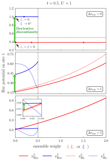
Figure 1: Exact Hxc and EEXX-only (Hx) potentials on site 1 of the Hubbard dimer plotted as functions of the ensemble weights [$\xi_{-}$ for the ionization (in red) of the two-electron ground state and $\xi$ for the neutral excitation process (in blue)] for $U=2t=1$ and various external potential values. The derivative discontinuity that occurs when switching from one excitation process to the other is highlighted in green. The vertical black line at $\xi=1/2$ (dotted) indicates the TGOK equiesemble.

VI.3 Connection with regular ground-state DFT

In order to establish a clearer connection with conventional $N$-electron ground-state DFT (i.e., the $\bm{\xi}={\bf 0}$ limit of the theory), we adopt in this section a different perspective by using the general and exact IP expressions of Eq. (48), where the ensemble Hxc potential is defined up to a constant. Unlike in Sec. V, and the previous section, we do not impose any constraint on the latter constant. According to Eq. (48) [see also Eqs. (98) and (99)], the IPs of the $N$-electron ($N=2$ here) ground and first neutral singlet excited states can be expressed as follows when $\bm{\xi}={\bf 0}$,

$$I_{0}^{N} =-\tilde{\varepsilon}_{\rm H}+\left.\dfrac{\partial E_{\rm Hxc}^{\xi_{-}}[n_{\Psi_{0}^{N}}]}{\partial\xi_{-}}\right|_{\xi_{-}=0},$$ (77a)

$$I_{1}^{N} =-\tilde{\varepsilon}_{\rm L}+\left.\dfrac{\partial E_{\rm Hxc}^{\bm{\xi}}[n_{\Psi_{0}^{N}}]}{\partial\xi_{-}}\right|_{\xi_{-}=0}-\left.\dfrac{\partial E_{\rm Hxc}^{\bm{\xi}}[n_{\Psi_{0}^{N}}]}{\partial\xi}\right|_{\xi=0},$$ (77b)

respectively, in terms of the regular (defined up to a constant) KS HOMO and LUMO energies ${\varepsilon}_{i}$ to which we have applied the Levy–Zahariev (LZ) density-functional shift in potential Levy and Zahariev (2014)

$$C[n]=\dfrac{E_{\rm Hxc}[n]-\int d\mathbf{r}\,v_{\rm Hxc}(\mathbf{r})n(\mathbf{r})}{N},$$ (78)

where $E_{\rm Hxc}[n]$ and $v_{\rm Hxc}(\mathbf{r})$ are the regular Hxc functional and potential, respectively:

$${\varepsilon}_{i}\rightarrow\tilde{\varepsilon}_{i}={\varepsilon}_{i}+C[n_{\Psi_{0}^{N}}].$$ (79)

The nice feature of LZ-shifted orbital energies is that they are invariant under constant shifts in the Hxc potential. In the present two-electron Hubbard dimer model [see Eqs. (64), (87), and (89)], the unshifted KS energies are $\varepsilon_{\rm H}=-\varepsilon_{\rm L}\equiv\varepsilon_{\rm H}(\Delta v_{\rm KS}^{\bm{\xi}={\bf 0}}(n_{\Psi_{0}^{N}}))$ and

$$C(n)=\dfrac{1}{2}[E_{\rm Hxc}(n)-(1-n)\Delta v_{\rm Hxc}(n)].$$ (80)

The top panel of Fig. 2 shows the variations in $U$ of the ground-state and first excited-state IPs at the exact and approximate EEXX levels of calculation in the asymmetric $\Delta v_{\rm ext}/t=2$ case. The trends of the ground-state IP in Fig. 2 are qualitatively the same as in Fig. 4 of Ref. Senjean and Fromager, 2018 (where $\Delta v_{\rm ext}/t=5$). As long as electron correlation is weak or moderately strong ($U/t\leq 2$), EEXX performs very well. In the stronger correlation regime, the relatively good performance of EEXX in the description of the excited-state IP was expected since, as readily seen from the following energy expressions Deur et al. (2017),

$$\dfrac{E_{0}^{N}}{U} =\dfrac{4}{\quantity(\frac{\Delta v_{\rm ext}}{U})^{2}-1}\left(\dfrac{t}{U}\right)^{2}+\mathcal{O}\left[\left(\dfrac{t}{U}\right)^{3}\right],$$ (81a)

$$\dfrac{E_{1}^{N}}{U} =1-\dfrac{\Delta v_{\rm ext}}{U}+\dfrac{2}{1-\frac{\Delta v_{\rm ext}}{U}}\left(\dfrac{t}{U}\right)^{2}+\mathcal{O}\left[\left(\dfrac{t}{U}\right)^{3}\right],$$ (81b)

for $U\gg\Delta v_{\rm ext}\gg t$, the first (singlet) excited state has essentially no correlation energy. This is not the case for the ground state, which explains the poor performance of EEXX in the description of the ground-state IP when electron correlation is strong.

For completeness (the following analysis has already been done for the ground-state IP in Ref. Senjean and Fromager, 2018), the decomposition into LZ-shifted KS LUMO energy and ensemble Hxc weight derivatives of the excited-state IP [see Eq. (77b)] is plotted as a function of the interaction strength $U$ in the bottom panel of Fig. 2. As $U$ increases, the Hxc ensemble weight derivatives dominate while the LZ-shifted LUMO energy essentially tends to the hopping parameter $t$, which is the expected result for a perfectly symmetric dimer. Indeed, the ground-state density approaches the value $n=1$ when $U/\Delta v_{\rm ext}$ becomes large Deur et al. (2017, 2018). Note that, at the EEXX level of approximation, the LZ-shifted LUMO energy is overestimated while the (absolute value of the) total weight derivatives contribution is underestimated, so that the errors mostly cancel out when evaluating the total excited-state IP (see the top panel of Fig. 2). Let us stress that, in the present case, being able to model the weight dependence of the ensemble density-functional exchange energy is essential.

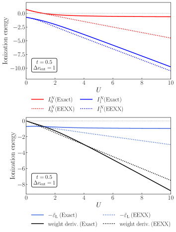
Figure 2: Top: Variation of ground-state (red) and excited-state (blue) IPs with the on-site repulsion $U$ in the asymmetric two-electron Hubbard dimer ($N=2$ and $\Delta v_{\rm ext}/t=2$). EEXX-only results (dotted lines) are shown for analysis purposes. Bottom: Decomposition of the excited-state IP into LZ-shifted KS LUMO energy and ensemble weight derivatives contributions [see Eq. (77b)].

For analysis purposes, we finally consider deviations from regular ground-state DFT that are more than infinitesimal by increasing the weight assigned to the ionized ground state ($\xi_{-}>0$) while remaining infinitesimally close to the ground-state limit (i.e., $\xi\rightarrow 0^{+}$) for the description of the excited state. The impact on the evaluation of both ground- and excited-state IPs, as well as the optical gap, is shown in Fig. 3. In the symmetric case (top panels), $I_{0}^{N}=-t-\frac{1}{2}(U-\sqrt{U^{2}+16t^{2}})$, which gives the lower value $I_{0}^{N}\approx t-\frac{U}{2}$ (i.e., $I_{0}^{N}\approx 0$ in Fig. 3, since $U=2t$) within the EEXX-only approximation, where the correlation energy of the two-electron ground state is missing. Since the exact excited-state IP $I^{N}_{1}=-t-U$ is recovered at the EEXX level in this case, the underestimation of the optical gap is solely due to the missing correlation in the ground state.

Turning on asymmetry ($\Delta v_{\rm ext}=1$) while remaining in the same moderately correlated regime ($U=2t$) introduces curvature in $\xi_{-}$ for both ground- and excited-state approximate EEXX IPs (see the middle left panel of Fig. 3). Note that, in the present case ($U=\Delta v_{\rm ext}=2t=1$), a perfect – and probably fortuitous – compensation of errors on both IPs occurs when computing the EEXX optical gap for the specific weight value of $\xi_{-}\approx 1.3$. In the stronger correlation regime ($U=5$), the curvature of EEXX IPs is further enhanced and perfect error cancellation does not occur anymore (see the bottom panels of Fig. 3). Unlike in the exact theory, the EEXX density-functional corrections to the bare weight-dependent KS IPs [see Eq. (48)] do not lead to weight-independent physical IPs. Nevertheless, as shown analytically in Appendix B, the EEXX functional succeeds in reversing, through its weight dependence, the variations in $\xi_{-}$ of both ground- and first excited-state KS IPs, thus avoiding a further underestimation of the excited-state IP as $\xi_{-}$ increases (see the bottom left panel of Fig. 3). As expected in such a strongly correlated regime, a sensible optical gap can only be obtained by retrieving the weight-dependent ensemble correlation energy, which is completely neglected at the EEXX level of approximation (see the bottom right panel of Fig. 3).

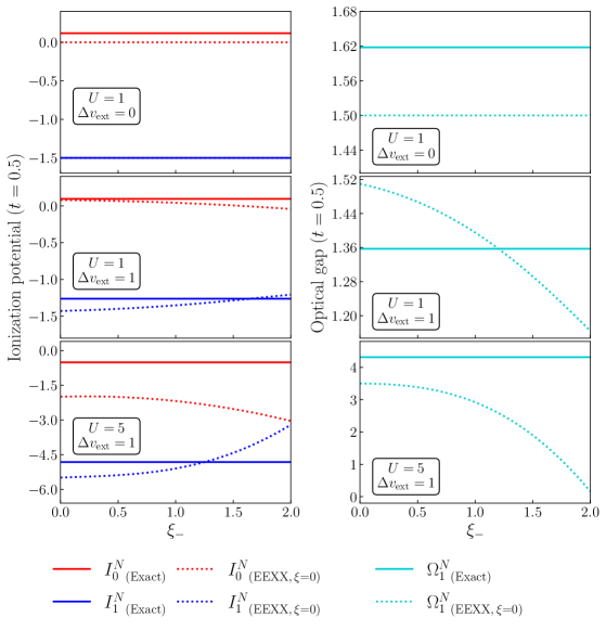
Figure 3: Left panels: Exact and EEXX-only IPs for the ground state (red curves) and the excited state (blue curves) plotted as functions of the ionization ensemble weight $\xi_{-}$ in the limit $\xi=0$ for the symmetric (top), and two asymmetric (middle, bottom) Hubbard dimers. Right panels: Exact and EEXX-only optical gaps plotted as the difference between the two IPs for the same three Hubbard dimers.

VII Conclusions and outlook

A unified ensemble DFT, where TGOK-DFT Theophilou (1979); Gross et al. (1988a) and the more recent $N$-centered ensemble DFT Senjean and Fromager (2018, 2020) have been merged — thus allowing for an in-principle exact density-functional description of both charged and neutral excitation processes from a single theory — has been derived [see the general excitation energy expression of Eq. (46)]. It is referred to as extended $N$-centered ensemble DFT. Unlike conventional DFT, in extended $N$-centered ensemble DFT, the number of electrons is artificially held constant and equal to the integer (so-called central) number of electrons $N$ of the reference ground state, even when the ensemble under study contains charged excited states in addition to neutral ones, hence the name of the theory. Therefore, and most importantly, the Hxc potential is always defined up to a constant shift within the present formalism.

The concept of derivative discontinuity for neutral excitations, which is much less discussed in the literature Levy (1995); Yang et al. (2014); Gould et al. (2022) than for charged excitations, has been revisited in this context. When adjusting, for each ground and excited $N$-electron states separately, the constant shift in the Hxc potential, such that each of them satisfies an exact ionization Koopmans’ theorem [see Eq. (49)], a jump (the so-called derivative discontinuity) is indeed observed when switching from the ground to the excited state of interest [see Eq. (57)].

Unlike in previous works, the asymptotic behavior of the density is never invoked nor used in the mathematical construction of the derivative discontinuities. It fully relies, instead, on the weight dependence of the extended $N$-centered ensemble Hxc density-functional energy. This allows for a straightforward application of the theory to lattice models (the Hubbard dimer in the present work). It may also open new perspectives in the description of gaps in mesoscopic systems Nazarov (2021). In principle, the present density-functional formalism is general enough to describe excitonic effects (through the inclusion of anionic states into the ensemble), as well as the challenging multiple-electron neutral excitation processes.

Finally, efforts should now be put into the design of weight-dependent density-functional approximations, which is essential for turning the theory into a reliable computational method. The (in-principle orbital-dependent) ensemble exact-exchange functional that we studied within the Hubbard dimer model nicely incorporates weight dependencies but it obviously needs a proper (weight-dependent) correlation counterpart whose construction is far from trivial Loos and Fromager (2020); Gould and Pittalis (2019); Fromager (2020). Exploring further the extension of ensemble DFT to the time-dependent linear response regime Gould et al. (2020), for example, could be a source of inspiration for this task. Work in these directions is currently in progress.

Appendix A Technical details about the application of e$N$-centered ensemble DFT on the Hubbard dimer

A.1 Ensemble functionals

In the following appendix, the exact and EEXX-approximate density functionals of the Hubbard dimer are systematically derived for the e$N$-centered ensemble in Sec. VI.

A.1.1 Exact functionals

We first consider the universal e$N$-centered ensemble density functional of the interacting system. As stated in Sec. VI.1, the central number of electrons was set to ${N=2}$. For this particular choice, all individual $N$- and $(N-1)$-electron energies of the Hubbard dimer have analytical expressions, which are available in, for example, Refs. Deur et al., 2017; Senjean and Fromager, 2018.

The e$N$-centered ensemble energy reads as

$$\begin{split}E^{\bm{\xi}}(\Delta v_{\rm ext})&=\left(1-\dfrac{\xi_{-}}{2}-\xi\right)E_{0}^{N}(\Delta v_{\rm ext})\\ &+\xi_{-}E_{0}^{N-1}(\Delta v_{\rm ext})+\xi E_{1}^{N}(\Delta v_{\rm ext}),\end{split}$$ (82)

where the dependence of individual energies on $t$ and $U$ has been omitted for clarity, which will also be the case for other expressions dependent on $t$ and $U$. The corresponding ensemble density reads as

$$\begin{split}n^{\bm{\xi}}:=n^{\bm{\xi}}(\Delta v_{\rm ext})&=\left(1-\dfrac{\xi_{-}}{2}-\xi\right)n_{\Psi_{0}^{N}}(\Delta v_{\rm ext})\\ &+\xi_{-}n_{\Psi_{0}^{N-1}}(\Delta v_{\rm ext})+\xi n_{\Psi_{1}^{N}}(\Delta v_{\rm ext}),\end{split}$$ (83)

where individual $N$- and $(N-1)$-electron densities can be straightforwardly obtained from first-order derivatives of individual energies with respect to the external potential. If we introduce the counting operator $\hat{N}=\sum_{i=0}^{1}\hat{n}_{i}$, it follows from Eq. (59c) and the Hellmann-Feynman theorem that

$$\begin{split}\dfrac{\partial E_{I}^{M}(\Delta v_{\rm ext})}{\partial\Delta v_{\rm ext}}&=\left\langle\Psi_{I}^{M}\right|\dfrac{\partial\hat{H}(\Delta v_{\rm ext})}{\partial\Delta v_{\rm ext}}\left|\Psi_{I}^{M}\right\rangle\\ &=\left\langle\Psi_{I}^{M}\right|\dfrac{1}{2}(\hat{N}-2\hat{n}_{0})\left|\Psi_{I}^{M}\right\rangle\\ &=\dfrac{M}{2}-n_{\Psi_{I}^{M}}(\Delta v_{\rm ext}),\end{split}$$ (84)

where $M=N-1$ or $N$, and $I=0$ or $1$.

In the practical calculations reported in Sec. VI, we rely on the Legendre-Fenchel transform definition of the universal e$N$-centered ensemble density functional, which can be obtained by analogy with TGOK-DFT Deur et al. (2017) and $N$-centered eDFT Senjean and Fromager (2018),

$$F^{\bm{\xi}}(n)=\sup_{\Delta v}\biggl{\{}E^{\bm{\xi}}(\Delta v)+\Delta v(n-1)\biggr{\}}.$$ (85)

In the above equation, the maximizing potential $\Delta v^{\bm{\xi}}(n)$ is equal to the derivative of $F^{\bm{\xi}}(n)$ with respect to the density,

$$\dfrac{\partial F^{\bm{\xi}}(n)}{\partial n}=\Delta v^{\bm{\xi}}(n).$$ (86)

Despite lacking a closed-form expression as a function of the density, the value of $F^{\bm{\xi}}(n)$ can still be computed to arbitrary accuracy for any given density from Eq. (85) via Lieb maximization. However, for the exact ensemble density $n^{\bm{\xi}}$ which is used in all calculations in Sec. VI, the maximizing potential is simply equal to the external potential, $\Delta v^{\bm{\xi}}(n^{\bm{\xi}})=\Delta v_{\rm ext}$, and $F^{\bm{\xi}}(n^{\bm{\xi}})=E^{\bm{\xi}}(\Delta v_{\rm ext})+\Delta v_{\rm ext}[n^{\bm{\xi}}(\Delta v_{\rm ext})-1]$ is an analytical function of $\Delta v_{\rm ext}$.

Next, we consider the noninteracting (KS) system which reproduces the e$N$-centered ensemble density of the interacting system. From the KS Hamiltonian

$$\hat{H}^{\rm KS}(\Delta v)=\hat{\mathcal{T}}+\frac{\Delta v}{2}(\hat{n}_{1}-\hat{n}_{0}),$$ (87)

we obtain the e$N$-centered ensemble energy as

$$\begin{split}\mathcal{E}_{\rm KS}^{\bm{\xi}}(\Delta v)&=\left(1-\xi-\frac{\xi_{-}}{2}\right)\mathcal{E}_{0}^{N}(\Delta v)\\ &+{\xi_{-}}\mathcal{E}_{0}^{N-1}(\Delta v)+\xi\mathcal{E}_{1}^{N}(\Delta v),\end{split}$$ (88)

with the $N$- and ($N-1$)-electron ground-state energies, and the $N$-electron excited state energy written as $\mathcal{E}_{0}^{N}(\Delta v)=2\varepsilon_{\rm H}(\Delta v)$, $\mathcal{E}_{0}^{N-1}(\Delta v)=\varepsilon_{\rm H}(\Delta v)$, and $\mathcal{E}_{1}^{N}(\Delta v)=0$, respectively, where

$$\varepsilon_{\rm H}(\Delta v)=-\sqrt{t^{2}+\dfrac{\Delta v^{2}}{4}}.$$ (89)

Similarly to the universal functional in Eq. (85), the noninteracting kinetic energy $T^{\bm{\xi}}_{\rm s}(n)$ can be written as a Legendre-Fenchel transform, which reads

$$T^{\bm{\xi}}_{\rm s}(n)=\sup_{\Delta v}\biggl{\{}2(1-\xi)\varepsilon_{\rm H}(\Delta v)-\Delta v(1-n)\biggr{\}}.$$ (90)

Since Eq. (90) is explicitly independent of the ensemble weight for the ($N-1$)-electron ground state $\xi_{-}$, it follows that the maximizing KS potential corresponding to the noninteracting e$N$-centered ensemble is the same one as in TGOK-DFT Deur et al. (2017). Hence, it can be expressed as follows,

$$\Delta v^{{\rm KS},\bm{\xi}}(n)\equiv\Delta v^{{\rm KS},\xi}(n)=\dfrac{2t(n-1)}{\sqrt{(1-\xi)^{2}-(1-n)^{2}}},$$ (91)

which implies that a given density $n$ is noninteracting e$N$-centered ensemble $v$-representable iff $\absolutevalue{n-1}\leq 1-\xi$. By plugging Eq. (91) into Eq. (90), we obtain the expression for the noninteracting kinetic energy functional, $T_{\rm s}^{\bm{\xi}}(n)$, as given in Eq. (61a).

Finally, the ensemble weight derivatives of Hxc functional $E_{\rm Hxc}^{\bm{\xi}}(n)=F^{\bm{\xi}}(n)-T_{\rm s}^{\bm{\xi}}(n)$, which are key ingredients for obtaining exact expressions for the IPs and the optical gap, are obtained as follows,

$$\begin{split}\dfrac{\partial E_{\rm Hxc}^{\bm{\xi}}(n)}{\partial\xi}&=E_{1}^{N}(\Delta v^{\bm{\xi}}(n))-E_{0}^{N}(\Delta v^{\bm{\xi}}(n))\\ &-\dfrac{2t(1-\xi)}{\sqrt{(1-\xi)^{2}-(1-n)^{2}}},\end{split}$$ (92)

and

$$\dfrac{\partial E_{\rm Hxc}^{\bm{\xi}}(n)}{\partial\xi_{-}}=E_{0}^{N-1}(\Delta v^{\bm{\xi}}(n))-\dfrac{E_{0}^{N}(\Delta v^{\bm{\xi}}(n))}{2}.$$ (93)

A.1.2 EEXX functional

The e$N$-centered ensemble exact (Hartree) exchange (EEXX) functional can be obtained from the formal expression of the Hx energy:

$$E_{\rm Hx}^{\bm{\xi}}(n)=U\left.\dfrac{\partial F^{\bm{\xi}}(n)}{\partial U}\right|_{U=0},$$ (94)

where we have, according to Eq. (85),

$$\begin{split}\left.\dfrac{\partial F^{\bm{\xi}}(n)}{\partial U}\right|_{U=0}&=\left(1-\dfrac{\xi_{-}}{2}-\xi\right)\left.\dfrac{\partial E_{0}^{N}(\Delta v)}{\partial U}\right|_{U=0,\Delta v=\Delta v_{\rm KS}^{\bm{\xi}}(n)}\\ &+\left.\xi\dfrac{\partial E_{1}^{N}(\Delta v)}{\partial U}\right|_{U=0,\Delta v=\Delta v_{\rm KS}^{\bm{\xi}}(n)},\end{split}$$ (95)

and, according to Eqs. (89) and (91), and Eq. (A7) in Deur et al. (2017),

$$\left.\dfrac{\partial E_{I}^{N}(\Delta v)}{\partial U}\right|_{U=0,\Delta v=\Delta v_{\rm KS}^{\bm{\xi}}(n)}\\ =\dfrac{I+1}{2}\left[1+\left(1-2I\right)\left(\dfrac{1-n}{1-\xi}\right)^{2}\right],$$ (96)

for $I=0$ or $1$. Finally, inserting Eq. (96) into Eq. (94) gives, after some rearrangements of various terms, the following expression for Hx energy of Eq. (61b)

$$E_{\rm Hx}^{\bm{\xi}}(n)=\dfrac{U}{2}\left[1+\xi-\dfrac{\xi_{-}}{2}+\left(1-3\xi-\dfrac{\xi_{-}}{2}\right)\left(\dfrac{1-n}{1-\xi}\right)^{2}\right].$$ (97)

A.2 Derivative discontinuity in the Hubbard dimer from the e$N$-centered ensemble perspective

A.2.1 General expressions

Within the formalism of extended $N$-centered ensembles, the derivative discontinuity can be shown to appear even in the Hubbard dimer. Starting from Eq. (48), we derive expressions for the IPs of the ground and the first excited state,

$$\begin{split}E^{N-1}_{0}-E^{N}_{0}=&-\varepsilon^{\bm{\xi}}_{\rm H}\\ &-\dfrac{1}{2}\left(E_{\rm Hxc}^{\bm{\xi}}(n^{\bm{\xi}})-\sum_{i=0}^{1}v_{{\rm Hxc},i}^{\bm{\xi}}n^{\bm{\xi}}_{i}\right)\\ &+\left(1+\dfrac{\xi_{-}}{2}\right)\left.\dfrac{\partial E_{\rm Hxc}^{\bm{\xi}}(n)}{\partial\xi_{-}}\right|_{n=n^{\bm{\xi}}}\\ &+\dfrac{\xi}{2}\left.\dfrac{\partial E_{\rm Hxc}^{\bm{\xi}}(n)}{\partial\xi}\right|_{n=n^{\bm{\xi}}},\end{split}$$ (98)

and

$$\begin{split}E^{N-1}_{0}-E^{N}_{1}=&-\varepsilon^{\bm{\xi}}_{\rm L}\\ &-\dfrac{1}{2}\left(E_{\rm Hxc}^{\bm{\xi}}(n^{\bm{\xi}})-\sum_{i=0}^{1}v_{{\rm Hxc},i}^{\bm{\xi}}n^{\bm{\xi}}_{i}\right)\\ &+\left(1+\dfrac{\xi_{-}}{2}\right)\left.\dfrac{\partial E_{\rm Hxc}^{\bm{\xi}}(n)}{\partial\xi_{-}}\right|_{n=n^{\bm{\xi}}}\\ &+\left(\dfrac{\xi}{2}-1\right)\left.\dfrac{\partial E_{\rm Hxc}^{\bm{\xi}}(n)}{\partial\xi}\right|_{n=n^{\bm{\xi}}},\end{split}$$ (99)

where the integral $\int d\mathbf{r}v_{\rm Hxc}^{\bm{\xi}}(\mathbf{r})n^{\bm{\xi}}(\mathbf{r})$ has been replaced by a summation over lattice sites. For the purpose of displaying the derivative discontinuity, the KS Hamiltonian of the Hubbard dimer is written with the KS potential determined up to a constant as follows,

$$\hat{H}^{{\rm KS},\bm{\xi}}=\hat{\mathcal{T}}+v^{{\rm KS},\bm{\xi}}_{1}\hat{n}_{1}+v^{{\rm KS},\bm{\xi}}_{0}\hat{n}_{0},$$ (100)

where

$$v^{{\rm KS},\bm{\xi}}_{i} =\frac{(-1)^{i-1}}{2}\Delta v^{{\rm KS},\bm{\xi}}-\mu^{\bm{\xi}}_{\rm Hxc},$$ (101a)

$$\Delta v^{{\rm KS},\bm{\xi}} =\left.\partial T^{\bm{\xi}}_{\rm s}(n)/\partial n\right|_{n=n^{\bm{\xi}}}\equiv\Delta v_{\rm ext}+\Delta v^{\bm{\xi}}_{\rm Hxc},$$ (101b)

and $n^{\bm{\xi}}$ is the exact e$N$-centered ensemble occupation of site 0. The total Hxc potential on site $i$ reads

$$v^{\bm{\xi}}_{{\rm Hxc},i}=\frac{(-1)^{i-1}}{2}\Delta v^{\bm{\xi}}_{\rm Hxc}-\mu^{\bm{\xi}}_{\rm Hxc}.$$ (102)

The constant shift, $-\mu^{\bm{\xi}}_{\rm Hxc}$, is determined to fulfill the constraint for exactification of Koopmans’ theorem in Eq. (49).

In order to derive the derivative discontinuity, we consider two specific ensembles. The first ensemble is the regular $N$-centered ensemble, where the ensemble weights take the values of $\xi=0$ and $0\leq\xi_{-}\leq 2$, describing the ionization process from the two-electron ground state, with the IP ${I_{0}^{N}=E_{0}^{N-1}-E_{0}^{N}}$. To fulfill Koopman’s theorem for the ground-state IP, we set all the terms on the right-hand sides of Eq. (98) to zero, except the HOMO energy. This gives the following constraint for the Hxc potential in the Hubbard dimer,

$$\sum_{i=0}^{1}v_{{\rm Hxc},i}^{(0,\xi_{-})}n^{\xi_{-}}_{i}=E^{\xi_{-}}_{\rm Hxc}(n^{\xi_{-}})-\left(2+\xi_{-}\right)\left.\dfrac{\partial E_{\rm Hxc}^{\xi_{-}}(n)}{\partial\xi_{-}}\right|_{n=n^{\xi_{-}}},$$ (103)

where $n^{\xi_{-}}=n^{(0,\xi_{-})}$ and $E_{\rm Hxc}^{\xi_{-}}=E_{\rm Hxc}^{(0,\xi_{-})}$. By inserting Eq. (102) into the above equation, and solving for $-\mu^{(0,\xi_{-})}_{\rm Hxc}$, we get

$$\begin{split}-\mu_{\rm Hxc}^{(0,\xi_{-})}&=\frac{1}{2}\left(\Delta v_{\rm Hxc}^{\xi_{-}}[n^{\xi_{-}}-1]+E_{\rm Hxc}^{\xi_{-}}(n^{\xi_{-}})\right)\\ &-\dfrac{2+\xi_{-}}{2}\left.\dfrac{\partial E_{\rm xc}^{\xi_{-}}(n)}{\partial\xi_{-}}\right|_{n=n^{\xi_{-}}},\end{split}$$ (104)

where, according to Eqs. (63) and (64), $\Delta v_{\rm Hxc}^{\xi_{-}}=\Delta v_{\rm Hxc}^{(0,\xi_{-})}(n^{\xi_{-}})=\Delta v_{\rm Hxc}^{(0,0)}(n^{\xi_{-}})$.

The second ensemble is the extended $N$-centered ensemble from Sec. VI, with the full weight range for the neutral excitation ($0<\xi\leq 1/2$), and the infinitesimal limit for the ionization from the two-electron ground state, i.e. $\xi_{-}\rightarrow 0^{+}$. The latter weight limit is imposed so that Koopmans’ theorem for the excited-state IP $I_{1}^{N}=E_{0}^{N-1}-E_{1}^{N}$ can still be fulfilled. By setting all the terms on the right-hand side of Eq. (99) to zero, except the LUMO energy, we get

$$\begin{split}\sum_{i=0}^{1}v_{{\rm Hxc},i}^{(\xi,0^{+})}n^{\xi}_{i}&=E_{\rm Hxc}^{\xi}(n^{\xi})+(2-\xi)\left.\dfrac{\partial E_{\rm xc}^{\xi}(n)}{\partial\xi}\right|_{n=n^{\xi}}\\ &-2\left.\dfrac{\partial E_{\rm xc}^{(\xi,\xi_{-})}(n^{\xi})}{\partial\xi_{-}}\right|_{\xi_{-}=0},\end{split}$$ (105)

where $n^{\xi}=n^{(\xi,0)}$ and $E_{\rm Hxc}^{\xi}=E_{\rm Hxc}^{(\xi,0)}$. After inserting Eq. (102) into the above equation, and solving for $-\mu^{(\xi,0^{+})}_{\rm Hxc}$, we get

$$\begin{split}-\mu_{\rm Hxc}^{(\xi,0^{+})}&=\frac{1}{2}\left(\Delta v_{\rm Hxc}^{\xi}[n^{\xi}-1]+E_{\rm Hxc}^{\xi}(n^{\xi})\right)\\ &+\dfrac{2-\xi}{2}\left.\dfrac{\partial E_{\rm xc}^{\xi}(n)}{\partial\xi}\right|_{n=n^{\xi}}-\left.\dfrac{\partial E_{\rm xc}^{(\xi,\xi_{-})}(n)}{\partial\xi_{-}}\right|_{\xi_{-}=0},\end{split}$$ (106)

where $\Delta v_{\rm Hxc}^{\xi}=\Delta v_{\rm Hxc}^{(\xi,0)}(n^{\xi})$. Considering now Eq. (104), the limit $\xi_{-}\rightarrow 0^{+}$ determines the value of the constant Hxc shift for the two-electron ground state,

$$\begin{split}-\mu_{\rm Hxc}^{(\xi=0,0^{+})}&=\dfrac{1}{2}\left(\Delta v_{\rm Hxc}[n_{\Psi_{0}^{N}}-1]+E_{\rm Hxc}(n_{\Psi_{0}^{N}})\right)\\ &-\left.\dfrac{\partial E_{\rm xc}^{\xi_{-}}(n_{\Psi_{0}^{N}})}{\partial\xi_{-}}\right|_{\xi_{-}=0}.\end{split}$$ (107)

In the case of Eq. (106), the limit $\xi\rightarrow 0^{+}$ returns the value of the Hxc shift for the TGOK ensemble with an infinitesimal amount of neutral excitation from the two-electron ground state.

$$\begin{split}-\mu_{\rm Hxc}^{(\xi\rightarrow 0^{+},0^{+})}&=\dfrac{1}{2}\left(\Delta v_{\rm Hxc}[n_{\Psi_{0}^{N}}-1]+E_{\rm Hxc}(n_{\Psi_{0}^{N}})\right)\\ &+\left.\dfrac{\partial E_{\rm xc}^{\xi}(n_{\Psi_{0}^{N}})}{\partial\xi}\right|_{\xi=0}-\left.\dfrac{\partial E_{\rm xc}^{\xi_{-}}(n_{\Psi_{0}^{N}})}{\partial\xi_{-}}\right|_{\xi_{-}=0}\end{split}$$ (108)

By subtracting Eq. (107) from Eq. (108) and using Eq. (102), we obtain the following expression for the derivative discontinuity,

$$\begin{split}v_{{\rm Hxc},1}^{(\xi\rightarrow 0^{+},0^{+})}-v_{{\rm Hxc},1}^{(\xi=0,0^{+})}&=\mu_{\rm Hxc}^{(\xi=0,0^{+})}-\mu_{\rm Hxc}^{(\xi\rightarrow 0^{+},0^{+})}\\ &=\left.\dfrac{\partial E_{\rm xc}^{\xi}(n_{\Psi_{0}^{N}})}{\partial\xi}\right|_{\xi=0}.\end{split}$$ (109)

This is an exact result for the derivative discontinuity in the Hubbard dimer, which is shown in Fig. 1.

A.2.2 Symmetric Hubbard dimer

In the symmetric dimer, the Hxc potential and the derivative discontinuity have closed-form expressions. Starting from the formulae for individual $N$- and $(N-1)$-electron energies, ${E_{0}^{N}(\Delta v_{\rm ext}=0)=\tfrac{1}{2}(U-\sqrt{U^{2}+16t^{2}})}$, ${E_{1}^{N}(\Delta v_{\rm ext}=0)=U}$ and ${E_{0}^{N-1}(\Delta v_{\rm ext}=0)=-t}$, the universal and the noninteracting kinetic energy e$N$-centered ensemble density functionals are derived as follows,

$$\begin{split}F^{\bm{\xi}}(n=1)&=E^{\bm{\xi}}(\Delta v_{\rm ext}=0)\\ &=\left(1-\dfrac{\xi_{-}}{2}-\xi\right)\dfrac{U-\sqrt{U^{2}+16t^{2}}}{2}\\ &-\xi_{-}t+\xi U,\\ \end{split}$$ (110)

and

$$T_{\rm s}^{\bm{\xi}}(n=1)=-2t(1-\xi),$$ (111)

while the EEXX functional reads

$$E_{\rm Hx}^{\bm{\xi}}(n=1)=\dfrac{U}{2}\left(1-\frac{\xi_{-}}{2}+\xi\right).$$ (112)

For the regular $N$-centered ensemble ($\xi=0$ and ${0\leq\xi_{-}\leq 2}$), the Hxc functional reads

$$E_{\rm Hxc}^{\xi_{-}}(n=1)=\left(1-\dfrac{\xi_{-}}{2}\right)\dfrac{U-\sqrt{U^{2}+16t^{2}}}{2}-\xi_{-}t+2t,$$ (113)

which can also be expressed as

$$E_{\rm Hxc}^{\xi_{-}}(n=1)=-(2-\xi_{-})\dfrac{\partial E_{\rm Hxc}^{\xi_{-}}(n=1)}{\partial\xi_{-}}.$$ (114)

Inserting the above expression into Eq. (104), and taking into account that $\Delta v_{\rm Hxc}^{\xi_{-}}=0$, we obtain from Eq. (102) that

$$\begin{split}v_{{\rm Hxc},1}^{(0,\xi_{-})}&=-2\dfrac{\partial E_{\rm Hxc}^{\xi_{-}}(n=1)}{\partial\xi_{-}}\\ &=\frac{U+4t-\sqrt{U^{2}+16t^{2}}}{2}.\end{split}$$ (115)

Using the EEXX functional [see Eq. (112))] instead of the exact Hxc functional clearly gives the wrong result,

$$v_{{\rm Hx},1}^{(0,\xi_{-})}=U/2.$$ (116)

Upon inclusion of the neutral excitation into the ensemble ($0<\xi\leq 1/2$), we observe that the EEXX-only and the exact Hxc ensemble potentials coincide in the symmetric dimer. To demonstrate this, we first isolate the e$N$-centered ensemble correlation functional from Eqs. (110), (111) and (112):

$$\begin{split}E_{\rm c}^{\bm{\xi}}(n=1)&=F^{\bm{\xi}}(n=1)-T_{\rm s}^{\bm{\xi}}(n=1)-E_{\rm Hx}^{\bm{\xi}}(n=1)\\ &=\left(1-\dfrac{\xi_{-}}{2}-\xi\right)\dfrac{4t-\sqrt{U^{2}+16t^{2}}}{2},\end{split}$$ (117)

which can also be expressed as

$$\begin{split}E_{\rm c}^{\bm{\xi}}(n=1)=&-(2-\xi)\dfrac{\partial E_{\rm c}^{\bm{\xi}}(n=1)}{\partial\xi}\\ &+(2+\xi_{-})\dfrac{\partial E_{\rm c}^{\bm{\xi}}(n=1)}{\partial\xi_{-}}.\end{split}$$ (118)

In the particular case when $\xi_{-}\rightarrow 0^{+}$, we have

$$\begin{split}E_{\rm c}^{\xi}(n=1)=&-(2-\xi)\dfrac{\partial E_{\rm c}^{\xi}(n=1)}{\partial\xi}\\ &+\left.2\dfrac{\partial E_{\rm c}^{(\xi_{-},\xi)}(n=1)}{\partial\xi_{-}}\right|_{\xi_{-}=0}.\end{split}$$ (119)

By inserting the above expression into Eq. (106), we can see that the correlation part in the $E_{\rm Hxc}^{\bm{\xi}}(n=1)$ functional is canceled out by its weight derivatives, which implies that only exchange terms contribute to $v_{\rm Hxc}^{(\xi,0^{+})}$, giving the following result:

$$\begin{split}v_{{\rm Hxc},1}^{(\xi,0^{+})}&\equiv v_{{\rm Hx},1}^{(\xi,0^{+})}\\ &=\dfrac{1}{2}\left(\dfrac{U}{2}+2\dfrac{\partial E_{\rm Hx}^{\xi}(n=1)}{\partial\xi}\right)-\left.\dfrac{\partial E_{\rm Hx}^{\bm{\xi}}(n=1)}{\partial\xi-}\right|_{\xi_{-}=0}\\ &=U.\end{split}$$ (120)

Hence, according to Eqs. (115) and (120), the exact derivative discontinuity in the symmetric dimer reads

$$v_{{\rm Hxc},1}^{(\xi\rightarrow 0^{+},0^{+})}-v_{{\rm Hxc},1}^{(\xi=0,0^{+})}=\dfrac{U-4t+\sqrt{U^{2}+16t^{2}}}{2},$$ (121)

while the EEXX-only approximation, obtained from Eqs. (116) and (120), reads

$$v_{{\rm Hx},1}^{(\xi\rightarrow 0^{+},0^{+})}-v_{{\rm Hx},1}^{(\xi=0,0^{+})}=\dfrac{U}{2},$$ (122)

which is always lower than the exact derivative discontinuity.

Appendix B EEXX approximation applied to the Hubbard dimer with $U\gg\Delta v_{\rm ext}=2t=1$

In the strongly correlated regime $U\gg\Delta v_{\rm ext}=2t=1$, the ground-state density is very close to 1 Deur et al. (2017), while the one-electron ground-state density $n_{\Psi^{N-1}_{0}}$ (we recall that the central number of electrons is $N=2$ in the present model) fulfills, according to Eqs. (84) and (89),

$$\begin{split}\dfrac{\partial\varepsilon_{\rm H}(\Delta v_{\rm ext})}{\partial\Delta v_{\rm ext}}&=-\dfrac{\Delta v_{\rm ext}}{4\sqrt{t^{2}+(\Delta v^{2}_{\rm ext}/4)}}\\ &=\dfrac{1}{2}\quantity(1-2n_{\Psi^{N-1}_{0}}),\end{split}$$ (123)

or, equivalently, $n_{\Psi^{N-1}_{0}}=\frac{1}{2}(1+\frac{1}{\sqrt{2}})$, thus leading to the following expression for the ensemble density under study

$$\begin{split}n^{\xi_{-}}&=n^{(\xi=0,\xi_{-})}\\ &={\left(1-\frac{\xi_{-}}{2}\right)\times 1+\xi_{-}\times\frac{1}{2}\left(1+\frac{1}{\sqrt{2}}\right)}\\ &=1+\dfrac{\xi_{-}}{2\sqrt{2}}.\end{split}$$ (124)

As a result, the ensemble KS potential varies with $\xi_{-}$ as follows [see Eq. (64)],

$$\Delta v^{\xi_{-}}_{\rm KS}=\dfrac{2t\left(n^{\xi_{-}}-1\right)}{\sqrt{1-\left(n^{\xi_{-}}-1\right)^{2}}}=\dfrac{\xi_{-}}{\sqrt{8-\xi_{-}^{2}}},$$ (125)

and the KS HOMO/LUMO energies read

$$-\varepsilon_{\rm H}^{\xi_{-}}=\varepsilon_{\rm L}^{\xi_{-}}=\sqrt{t^{2}+\frac{\left(\Delta v^{\xi_{-}}_{\rm KS}\right)^{2}}{4}}=\dfrac{\sqrt{2}}{\sqrt{8-\xi_{-}^{2}}}.$$ (126)

Therefore, the bare KS ground-state (excited-state) IP increases (decreases) with the ensemble weight $\xi_{-}$, unlike the approximate interacting EEXX one (see the bottom left panel of Fig. 3).

In order to identify the origin of the latter trend we need to consider the decomposition of both IPs as given in Eq. (48). The Hxc potential term, which contributes to both IPs, reads

$$\begin{split}\dfrac{\Delta v^{\xi_{-}}_{\rm Hxc}}{2N}\left(2-2n^{\xi_{-}}\right)&=-\dfrac{\xi_{-}\left(\Delta v^{\xi_{-}}_{\rm KS}-\Delta v_{\rm ext}\right)}{4\sqrt{2}}\\ &=\dfrac{1}{4\sqrt{2}}\left(-\dfrac{\xi_{-}^{2}}{\sqrt{8-\xi_{-}^{2}}}+\xi_{-}\right),\end{split}$$ (127)

since $N=2$. Note that, as we approach the $\xi_{-}=2$ limit, the above contribution decreases with $\xi_{-}$. Therefore, the weight dependence of the approximate EEXX excited-state IP originates from the remaining ensemble Hx energy term and its weight derivatives. The contribution that is common to both ground- and excited-state IPs reads

$$I^{\xi_{-}}_{0,\rm Hx}=\left[-\dfrac{E^{\xi_{-}}_{\rm Hx}(n)}{N}+\left(1+\dfrac{\xi_{-}}{N}\right)\dfrac{\partial E^{\xi_{-}}_{\rm Hx}(n)}{\partial\xi_{-}}\right]_{n=n^{\xi_{-}}},$$ (128)

where [see Eq. (61b)]

$$E^{\xi_{-}}_{\rm Hx}(n)=\dfrac{U}{2}\left(1-\dfrac{\xi_{-}}{2}\right)\left[1+(n-1)^{2}\right],$$ (129)

thus leading to

$$I^{\xi_{-}}_{0,\rm Hx}=-\dfrac{U}{2}\left[1+(n^{\xi_{-}}-1)^{2}\right]=-\dfrac{U}{2}\left(1+\dfrac{\xi^{2}_{-}}{8}\right).$$ (130)

The above contribution is therefore responsible for the net decrease of the EEXX ground-state IP as the ensemble weight $\xi_{-}$ increases.

Turning to the excited-state IP, we need to consider the following additional contribution [see Eq. (48)]:

$$\begin{split}-\Delta_{\rm Hx}^{\xi_{-}}&=-\left.\dfrac{\partial E^{(\xi,\xi_{-})}_{\rm Hx}(n)}{\partial\xi}\right|_{\xi=0,n=n^{\xi_{-}}}\\ &=-\dfrac{U}{2}\left[1-(n^{\xi_{-}}-1)^{2}\left(1+\xi_{-}\right)\right]\\ &=-\dfrac{U}{2}\left[1-\dfrac{\xi_{-}^{2}\left(1+\xi_{-}\right)}{8}\right],\end{split}$$ (131)

which, when it is added to the remaining Hx contribution of Eq. (130), gives the total Hx term

$$I^{\xi_{-}}_{0,\rm Hx}-\Delta_{\rm Hx}^{\xi_{-}}=-\dfrac{U}{2}\left(2-\dfrac{\xi_{-}^{3}}{8}\right).$$ (132)

The above contribution is therefore responsible for the net increase with $\xi_{-}$ of the EEXX excited-state IP.

In summary, at the EEXX level of approximation and in the considered $U\gg\Delta v_{\rm ext}=2t=1$ regime, the ground- and first excited-state IPs read

$$I^{N}_{0}\approx\dfrac{1}{4\sqrt{2}}\left(\xi_{-}+\sqrt{8-\xi_{-}^{2}}\right)-\dfrac{U}{2}\left(1+\dfrac{\xi^{2}_{-}}{8}\right),$$ (133a)

$$I^{N}_{1}\approx\dfrac{1}{4\sqrt{2}}\left(\xi_{-}-\dfrac{8+\xi_{-}^{2}}{\sqrt{8-\xi_{-}^{2}}}\right)-\dfrac{U}{2}\left(2-\dfrac{\xi_{-}^{3}}{8}\right),$$ (133b)

respectively, thus leading to the following expression for the optical gap

$$\begin{split}I_{0}^{N}-I^{N}_{1}&\approx\dfrac{2\sqrt{2}}{\sqrt{8-\xi_{-}^{2}}}+\dfrac{U}{2}\left[1-\dfrac{\xi_{-}^{2}(1+\xi_{-})}{8}\right].\end{split}$$ (134)

As a result, we obtain in the limiting $\xi_{-}=0$ and $\xi_{-}=2$ cases the following expressions,

$$I^{N}_{0} \overset{\xi_{-}=0}{\approx}\dfrac{1}{2}-\dfrac{U}{2},$$ (135a)

$$I^{N}_{1} \overset{\xi_{-}=0}{\approx}-\dfrac{1}{2}+U,$$ (135b)

$$I^{N}_{0}-I^{N}_{1} \overset{\xi_{-}=0}{\approx}1+\frac{U}{2},$$ (135c)

and

$$I^{N}_{0} \overset{\xi_{-}=2}{\approx}\dfrac{1}{\sqrt{2}}-\frac{3U}{4},$$ (136a)

$$I^{N}_{1} \overset{\xi_{-}=2}{\approx}-\dfrac{1}{\sqrt{2}}-\frac{U}{2},$$ (136b)

$$I^{N}_{0}-I^{N}_{1} \overset{\xi_{-}=2}{\approx}\sqrt{2}-\frac{U}{4},$$ (136c)

respectively, which are in very good agreement with the values obtained numerically for $U=5$ (see the bottom panels of Fig. 3). Note that, in the latter case, the EEXX optical gap equals $\sqrt{2}-\frac{5}{4}\approx 0.16$ when $\xi_{-}=2$, which confirms the dramatic underestimation of the optical gap that is observed in the bottom right panel of Fig. 3 as $\xi_{-}$ increases.

References

- Kohn and Sham (1965) W. Kohn and L. Sham, Phys. Rev. 140, A1133 (1965).
- Casida and Huix-Rotllant (2012) M. Casida and M. Huix-Rotllant, Annu. Rev. Phys. Chem. 63, 287 (2012).
- Runge and Gross (1984) E. Runge and E. K. Gross, Phys. Rev. Lett. 52, 997 (1984).
- Onida et al. (2002) G. Onida, L. Reining, and A. Rubio, Rev. Mod. Phys. 74, 601 (2002).
- Martin et al. (2016) R. M. Martin, L. Reining, and D. M. Ceperley, Interacting Electrons: Theory and Computational Approaches (Cambridge University Press, 2016).
- Hedin (1965) L. Hedin, Phys. Rev. 139, A796 (1965).
- Golze et al. (2019) D. Golze, M. Dvorak, and P. Rinke, Front. Chem. 7, 377 (2019).
- Marie et al. (2023) A. Marie, A. Ammar, and P.-F. Loos, “The Approximation: A Quantum Chemistry Perspective,” (2023), arXiv:2311.05351 [physics.chem-ph] .
- Strinati (1988) G. Strinati, Riv. Nuovo Cimento 11, 1 (1988).
- Sottile et al. (2007) F. Sottile, M. Marsili, V. Olevano, and L. Reining, Phys. Rev. B 76, 161103 (2007).
- Blase et al. (2020) X. Blase, I. Duchemin, D. Jacquemin, and P.-F. Loos, J. Phys. Chem. Lett. 11, 7371 (2020).
- Fuks and Maitra (2014) J. I. Fuks and N. T. Maitra, Phys. Chem. Chem. Phys. 16, 14504 (2014).
- Maitra et al. (2004) N. T. Maitra, F. Zhang, R. J. Cave, and K. Burke, J. Chem. Phys. 120, 5932 (2004).
- Lacombe and Maitra (2023) L. Lacombe and N. Maitra, npj Comput Mater 9, 124 (2023).
- Pastorczak et al. (2013) E. Pastorczak, N. I. Gidopoulos, and K. Pernal, Phys. Rev. A 87, 062501 (2013).
- Pastorczak and Pernal (2014) E. Pastorczak and K. Pernal, J. Chem. Phys. 140, 18A514 (2014).
- Franck and Fromager (2014) O. Franck and E. Fromager, Mol. Phys. 112, 1684 (2014).
- Yang et al. (2014) Z.-h. Yang, J. R. Trail, A. Pribram-Jones, K. Burke, R. J. Needs, and C. A. Ullrich, Phys. Rev. A 90, 042501 (2014).
- Pribram-Jones et al. (2014) A. Pribram-Jones, Z. hui Yang, J. R.Trail, K. Burke, R. J.Needs, and C. A.Ullrich, J. Chem. Phys. 140, 18A541 (2014).
- Filatov (2015) M. Filatov, WIREs Comput. Mol. Sci. 5, 146 (2015).
- Senjean et al. (2015) B. Senjean, S. Knecht, H. J. Aa. Jensen, and E. Fromager, Phys. Rev. A 92, 012518 (2015).
- Deur et al. (2017) K. Deur, L. Mazouin, and E. Fromager, Phys. Rev. B 95, 035120 (2017).
- Yang et al. (2017) Z.-h. Yang, A. Pribram-Jones, K. Burke, and C. A. Ullrich, Phys. Rev. Lett. 119, 033003 (2017).
- Gould and Pittalis (2017) T. Gould and S. Pittalis, Phys. Rev. Lett. 119, 243001 (2017).
- Gould et al. (2018) T. Gould, L. Kronik, and S. Pittalis, J. Chem. Phys. 148, 174101 (2018).
- Deur et al. (2018) K. Deur, L. Mazouin, B. Senjean, and E. Fromager, Eur. Phys. J. B 91, 162 (2018).
- Gould and Pittalis (2019) T. Gould and S. Pittalis, Phys. Rev. Lett. 123, 016401 (2019).
- Fromager (2020) E. Fromager, Phys. Rev. Lett. 124, 243001 (2020).
- Gould et al. (2020) T. Gould, G. Stefanucci, and S. Pittalis, Phys. Rev. Lett. 125, 233001 (2020).
- Gould (2020) T. Gould, J. Phys. Chem. Lett. 11, 9907 (2020).
- Loos and Fromager (2020) P.-F. Loos and E. Fromager, J. Chem. Phys. 152, 214101 (2020).
- Gould and Kronik (2021) T. Gould and L. Kronik, J. Chem. Phys. 154, 094125 (2021).
- Gould and Pittalis (2023) T. Gould and S. Pittalis, “Local density approximation for excited states,” (2023), arXiv:2306.04023 [physics.chem-ph] .
- Gould et al. (2023) T. Gould, D. P. Kooi, P. Gori-Giorgi, and S. Pittalis, Phys. Rev. Lett. 130, 106401 (2023).
- Gould et al. (2022) T. Gould, Z. Hashimi, L. Kronik, and S. G. Dale, J. Phys. Chem. Lett. 13, 2452 (2022).
- Gould et al. (2021) T. Gould, L. Kronik, and S. Pittalis, Phys. Rev. A 104, 022803 (2021).
- Cernatic et al. (2022) F. Cernatic, B. Senjean, V. Robert, and E. Fromager, Top Curr Chem (Z) 380, 4 (2022).
- Theophilou (1979) A. K. Theophilou, J. Phys. C: Solid State Phys. 12, 5419 (1979).
- Theophilou (1987) A. K. Theophilou, “The single particle density in physics and chemistry,” (Academic Press, 1987) pp. 210–212.
- Gross et al. (1988a) E. K. U. Gross, L. N. Oliveira, and W. Kohn, Phys. Rev. A 37, 2809 (1988a).
- Schilling and Pittalis (2021) C. Schilling and S. Pittalis, Phys. Rev. Lett. 127, 023001 (2021).
- Liebert et al. (2022) J. Liebert, F. Castillo, J.-P. Labbé, and C. Schilling, J. Chem. Theory Comput. 18, 124 (2022).
- Benavides-Riveros et al. (2022) C. L. Benavides-Riveros, L. Chen, C. Schilling, S. Mantilla, and S. Pittalis, Phys. Rev. Lett. 129, 066401 (2022).
- Liebert and Schilling (2023a) J. Liebert and C. Schilling, New J. Phys. 25, 013009 (2023a).
- Liebert and Schilling (2023b) J. Liebert and C. Schilling, SciPost Phys. 14, 120 (2023b).
- Senjean and Fromager (2018) B. Senjean and E. Fromager, Phys. Rev. A 98, 022513 (2018).
- Senjean and Fromager (2020) B. Senjean and E. Fromager, Int. J. Quantum Chem. 120, e26190 (2020).
- Perdew et al. (1982) J. P. Perdew, R. G. Parr, M. Levy, and J. L. Balduz Jr, Phys. Rev. Lett. 49, 1691 (1982).
- Perdew and Levy (1983) J. P. Perdew and M. Levy, Phys. Rev. Lett. 51, 1884 (1983).
- Baerends et al. (2013) E. J. Baerends, O. V. Gritsenko, and R. Van Meer, Phys. Chem. Chem. Phys. 15, 16408 (2013).
- Baerends (2017) E. J. Baerends, Phys. Chem. Chem. Phys. 19, 15639 (2017).
- Baerends (2018) E. J. Baerends, J. Chem. Phys. 149, 054105 (2018).
- Baerends (2022) E. J. Baerends, Phys. Chem. Chem. Phys. 24, 12745 (2022).
- Baerends (2020) E. J. Baerends, Mol. Phys. 118, e1612955 (2020).
- Levy (1995) M. Levy, Phys. Rev. A 52, R4313 (1995).
- Deur and Fromager (2019) K. Deur and E. Fromager, J. Chem. Phys. 150, 094106 (2019).
- Gross et al. (1988b) E. K. U. Gross, L. N. Oliveira, and W. Kohn, Phys. Rev. A 37, 2805 (1988b).
- Levy (1979) M. Levy, Proc. Natl. Acad. Sci. 76, 6062 (1979).
- Lieb (1983) E. H. Lieb, Int. J. Quantum Chem. 24, 243 (1983).
- Teale et al. (2022) A. M. Teale, T. Helgaker, A. Savin, C. Adamo, B. Aradi, A. V. Arbuznikov, P. W. Ayers, E. J. Baerends, V. Barone, P. Calaminici, E. Cancès, E. A. Carter, P. K. Chattaraj, H. Chermette, I. Ciofini, T. D. Crawford, F. De Proft, J. F. Dobson, C. Draxl, T. Frauenheim, E. Fromager, P. Fuentealba, L. Gagliardi, G. Galli, J. Gao, P. Geerlings, N. Gidopoulos, P. M. W. Gill, P. Gori-Giorgi, A. Görling, T. Gould, S. Grimme, O. Gritsenko, H. J. A. Jensen, E. R. Johnson, R. O. Jones, M. Kaupp, A. M. Köster, L. Kronik, A. I. Krylov, S. Kvaal, A. Laestadius, M. Levy, M. Lewin, S. Liu, P.-F. Loos, N. T. Maitra, F. Neese, J. P. Perdew, K. Pernal, P. Pernot, P. Piecuch, E. Rebolini, L. Reining, P. Romaniello, A. Ruzsinszky, D. R. Salahub, M. Scheffler, P. Schwerdtfeger, V. N. Staroverov, J. Sun, E. Tellgren, D. J. Tozer, S. B. Trickey, C. A. Ullrich, A. Vela, G. Vignale, T. A. Wesolowski, X. Xu, and W. Yang, Phys. Chem. Chem. Phys. 24, 28700 (2022).
- Gidopoulos et al. (2002) N. I. Gidopoulos, P. G. Papaconstantinou, and E. K. U. Gross, Phys. Rev. Lett. 88, 033003 (2002).
- Hodgson et al. (2021) M. J. P. Hodgson, J. Wetherell, and E. Fromager, Phys. Rev. A 103, 012806 (2021).
- Levy and Zahariev (2014) M. Levy and F. Zahariev, Phys. Rev. Lett. 113, 113002 (2014).
- Sagredo and Burke (2018) F. Sagredo and K. Burke, J. Chem. Phys. 149, 134103 (2018).
- Marut et al. (2020) C. Marut, B. Senjean, E. Fromager, and P.-F. Loos, Faraday Discuss. 224, 402 (2020).
- Gould et al. (2019) T. Gould, S. Pittalis, J. Toulouse, E. Kraisler, and L. Kronik, Phys. Chem. Chem. Phys. 21, 19805 (2019).
- Carrascal et al. (2015) D. J. Carrascal, J. Ferrer, J. C. Smith, and K. Burke, J. Phys. Condens. Matter 27, 393001 (2015).
- Li et al. (2018) C. Li, R. Requist, and E. K. U. Gross, J. Chem. Phys. 148, 084110 (2018).
- Carrascal et al. (2018) D. J. Carrascal, J. Ferrer, N. Maitra, and K. Burke, Eur. Phys. J. B 91, 142 (2018).
- Smith et al. (2016) J. C. Smith, A. Pribram-Jones, and K. Burke, Phys. Rev. B 93, 245131 (2016).
- Giarrusso and Loos (2023) S. Giarrusso and P.-F. Loos, J. Phys. Chem. Lett. 14, 8780 (2023).
- Ullrich (2018) C. A. Ullrich, Phys. Rev. B 98, 035140 (2018).
- Scott et al. (2023) T. R. Scott, J. Kozlowski, S. Crisostomo, A. Pribram-Jones, and K. Burke, “Exact conditions for ensemble density functional theory,” (2023), arXiv:2307.00187 [cond-mat.str-el] .
- Sobrino et al. (2023) N. Sobrino, D. Jacob, and S. Kurth, J. Chem. Phys. 159, 154110 (2023).
- Liebert et al. (2023) J. Liebert, A. Y. Chaou, and C. Schilling, J. Chem. Phys. 158, 214108 (2023).
- Nazarov (2021) V. U. Nazarov, J. Chem. Phys. 155, 194105 (2021).