Production of para-true muonium in linearly polarized photon fusions

Abstract

True muonium (TM)—the bound state of $\mu^{+}\mu^{-}$, has not been discovered yet. It was demonstrated that searching TM via $\gamma\gamma$ fusions in heavy ion collisions is feasible due to the enhancement of the atom number. We study the production of the para-true muonium (pTM) in the collisions of linearly polarized photons in the experiments of ultra-peripheral nuclear collisions, calculate the production rate as well as the transverse spectrum of pTM, and explore the discovery potential in nuclear experiments. Our results show that there is a significant correlation between the linearly polarized photon distribution and the transverse momentum distribution of pTM. The optimal kinematic region of the generated pTM is identified, which can provide a theoretical guide to the detection of pTM in experiments.

The $\mu^{+}\mu^{-}$ bound state, referred to as true muonium (TM), is a short-lived, exotic atom-like particle composed of a muon and its antiparticle, the antimuon. It is a purely Quantum Electrodynamics (QED) bound state. The lightest QED atom, the positronium ($e^{+}e^{-}$ bound state), had been observed more than 75 years ago Deutsch:1951zza and studied extensively. Even the so-called muonium ($\mu e$ bound state) Hughes:1960zz , $\pi\mu$ atom Coombes:1976hi , and the dipositronium Cassidy:2007 ($(e^{+}e^{-})(e^{+}e^{-})$ molecule) have been discovered and studied more, while the TM has not yet been observed since its possible had been discussed Marshak:1947zz soon after the clarification of the leptonic nature of the muon Lattes:1947mw ; Lattes:1947mx ; Lattes:1947my in the middle of the last century. The investigation of TM can contribute to our broader understanding of the Standard Model of particle physics and may offer clues to the existence of physics beyond this well-established framework Jaeckel:2010xx ; Tucker-Smith:2010wdq ; Kopp:2014tsa ; Agrawal:2021dbo .

Muons are heavy, unstable relatives of electrons, with a mass approximately 207 times that of an electron. Due to the short lifetime of muons and their antimatter counterparts, TM exists only fleetingly Bilenkii:1969 ; Hughes:1971 ; Malenfant:1987tm ; Jentschura:1998vkm , making it challenging to study and observe directly. The muon’s relatively short lifetime, on the order of microseconds ParticleDataGroup:2022pth , restricts the timescale for the formation and stability of TM. Many sophisticated experimental techniques have been employed to detect and study these ephemeral particles, often relying on high-energy accelerators and advanced detection methods. It was proposed to detect the TM in the physical processes at high energy experimental apparatus, such as $\pi^{-}p\to(\mu^{+}\mu^{-})n$ Bilenkii:1969 , $\gamma Z\to(\mu^{+}\mu^{-})Z$ Bilenkii:1969 ; Francener:2021wzx , $eZ\to e(\mu^{+}\mu^{-})Z$ Arteaga-Romero:2000mwd ; Krachkov:2017afm ; Banburski:2012tk , $Z_{1}Z_{2}\to Z_{1}Z_{2}(\mu^{+}\mu^{-})$ Ginzburg:1998df ; Chen:2012ci ; Yu:2013uka ; Azevedo:2019hqp ; Yu:2022hdt ; Francener:2021wzx (where $Z$ indicates a heavy nucleus), $\mu^{+}\mu^{-}$ collisions Hughes:1971 , $\eta\to(\mu^{+}\mu^{-})\gamma$ Nemenov:1972 ; CidVidal:2019qub , $e^{+}e^{-}$ collisions Moffat:1975uw ; Brodsky:2009gx ; Gargiulo:2023tci , $K_{L}\to(\mu^{+}\mu^{-})\gamma$ Ji:2017lyh , etc. Among these processes, the $e^{+}e^{-}\to(\mu^{+}\mu^{-})$ and $\gamma(\mu^{+}\mu^{-})$ is of particular interest because there is no hadron involved and thus is a pure QED process. It was demonstrated in Ref. Brodsky:2009gx that the TM could be discovered at electron-positron colliders, if the $\mu^{+}\mu^{-}$ resonances above the threshold are also taken into account, because the states with high principal quantum numbers cannot be distinguished from the resonances just above the threshold due to the beam energy spread, which production rates are enhanced by the Sommerfeld-Schwinger-Sakharov factor Sommerfeld:1939 . Based on this, it was proposed to search for TM with Fool’s Intersection Storage Rings ($e^{+}e^{-}\to(\mu^{+}\mu^{-})$) discussed by Bjorken Bjorken:1976mk in which the electron and positron beams are arranged to merge at a small angle in order to give rise to a strong boost for the produced TM, and to search for the para-TM (pTM) and ortho-TM (oTM) using the initial and final radiation technology ($e^{+}e^{-}\to\gamma(\mu^{+}\mu^{-})$) on BESIII and Belle-II experiments Harris:2008tx ; Belle-II:2010dht .

Another promising process is the heavy ion collisions. If the heavy ions collide with impact parameter larger than the twice of the radius of the nuclei, i.e., the ultra-peripheral collisions (UPC), the strong interaction does not get involved, ensuring $\gamma\gamma$ fusion in UPC a QED dominant process Baltz:2007kq . The electro-magnetic field strength is scaled with the atom number $Z$. Hence comparing with electron-positron collisions, the production rate is enhanced by a factor $Z^{4}$ in $\gamma\gamma$ fusions in UPC. For example, in lead-lead collisions the rate will be enhanced by $82^{4}\sim 4.5\times 10^{7}$. This makes the study of rare processes possible in heavy-ion collisions. As a consequence, the light-by-light scattering, predicted by quantum theory but forbidden by classical electrodynamics, was observed in $\mathrm{Pb}+\mathrm{Pb}(\gamma\gamma)\to\mathrm{Pb}^{*}+\mathrm{Pb}^{*}+\gamma\gamma$ process by ATLAS ATLAS:2017fur .

One the theory side, the calculation can be carried out with the equivalent photon approximation where the virtual photons are regarded as quasi-real photons, which is also known as the Weizsäcker–Williams method Fermi:1924tc ; vonWeizsacker:1934nji ; Williams:1935dka . The quasi-photons, radiated from the relativistic nuclei, can be either unpolarized and linearly polarized. The linearly polarized photon distribution is correlated with the transverse momentum and the azimuthal distribution of the produced particles. It was proposed that the linearly polarized photon distribution can be extracted from the azimuthal-asymmetries of the lepton pair production in UPCs, see, e.g., Ref Li:2019yzy . The $\cos 4\phi$ asymmetry has been measured by STAR collaboration STAR:2019wlg .

The transverse momentum distribution provides useful information for experimental research. Although the total production rate of pTM in UPCs has been studied by previous works, however, the transverse momentum distribution of pTM has never been extensively explored, especially in the small transverse momentum region. Moreover, the effect of the linearly polarized photon is never explored. In this work, We will calculate the transverse momentum dependent differential cross-sections and study the effect of linearly polarized photons on the transverse momentum distribution of the pTM.

The pTM—the ${}^{1}S_{0}$ bound state of $\mu^{-}\mu^{+}$, can be produced by $\gamma\gamma$ fusion, which is shown in Fig. 1.

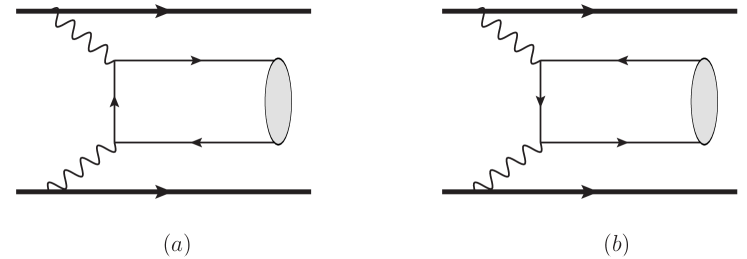
Figure 1: Production of para-true muonium via $\gamma\gamma$ fusion in heavy ion collisions.

When the virtuality of photon is small, one can utilize the equivalence photon approximation to calculate the differential cross section. In this work, we take the transverse momentum distribution of pTM into account. If the transverse momentum of pTM in the final state is small, the differential cross section takes the form

$$d\sigma= \frac{1}{2s}\frac{d^{3}\boldsymbol{q}}{(2\pi)^{3}2q^{0}}\int dx_{a}dx_{b}d^{2}\boldsymbol{p}_{aT}d^{2}\boldsymbol{p}_{bT}$$

$$(2\pi)^{4}\delta^{4}(p_{a}+p_{b}-q)\Gamma^{\mu\nu}_{A}(x_{a},\boldsymbol{p}_{aT})\Gamma^{\rho\sigma}_{B}(x_{b},\boldsymbol{p}_{bT})$$

$$\times H_{\mu\rho;\nu\sigma}(p_{a},p_{b};q),$$ (1)

where $\sqrt{s}$ is the collision energy per nucleus pair in the center-of-mass frame. $H$ is the partonic scattering amplitude of $\gamma\gamma\to\rm{pTM}$ times its complex conjugate, and $\Gamma_{A,B}$ is the photon correlation matrix of the nuclei $A$ and $B$, respectively, defined as the Fourier transform of the correlator of electromagnetic tensor as

$$\Gamma^{\mu\nu}(x,\boldsymbol{k}_{T})$$

$$= \int\frac{dz^{-}dz_{T}^{2}}{x^{2}P^{+}(2\pi)^{3}}e^{ik\cdot z}\langle P|F^{+\mu}(0)F^{+\nu}(z)|P\rangle|_{z^{+}=0}$$

$$= -\frac{1}{2x}g_{T}^{\mu\nu}f_{1}^{\gamma}(x,\boldsymbol{k}_{T}^{2})+\frac{1}{x}\left(\frac{1}{2}g^{\mu\nu}_{\perp}+\frac{k_{T}^{\mu}k_{T}^{\nu}}{\boldsymbol{k}_{T}^{2}}\right)h_{1}^{\perp\gamma}(x,\boldsymbol{k}_{T}^{2}),$$ (2)

where $g_{T}^{\mu\nu}=g^{\mu\nu}-n^{\mu}\bar{n}^{\nu}-n^{\nu}\bar{n}^{\mu}$ is the transverse metric and the light-cone vectors are $n=\frac{1}{\sqrt{2}}(1,0,0,-1)$ and $\bar{n}=\frac{1}{\sqrt{2}}(1,0,0,1)$. The transverse part of a vector $a$ is then expressed as $a_{T}^{\mu}=g_{T}^{\mu\nu}a_{\nu}$. $F^{\mu\nu}=\partial^{\mu}A^{\nu}-\partial^{\nu}A^{\mu}$ is the electromagnetic tensor, and $z=z^{-}\bar{n}+z_{T}$. Distinguished from the gluon case, there is no Wilson line. $f_{1}^{\gamma}$ is the unpolarized photon distribution function, while $h_{1}^{\perp\gamma}$ is the distribution of linearly polarized photons. The effect of $h_{1}^{\perp\gamma}$ has not be considered in the previous research of TM production. In general case, $h_{1}^{\perp\gamma}$ is independent of $f_{1}^{\gamma}$ but there is an upper bound $|h_{1}^{\perp\gamma}|\leq f_{1}^{\gamma}$. However, when the photons carry very small longitudinal momenta $k^{+}$, nearly all the photons are linearly polarized, in this case one has $h_{1}^{\perp\gamma}(x,\boldsymbol{k}_{T})\simeq f_{1}^{\gamma}(x,\boldsymbol{k}_{T})$ Li:2019yzy . This relation will be utilized in the numerical discussions.

The partonic scattering differential cross section of $\gamma\gamma\to\rm{pTM}$ can be expressed as

$$H_{\mu\rho;\nu\sigma}(p_{a},p_{b};q)=M_{\mu\rho}(p_{a},p_{b};q)M^{*}_{\nu\sigma}(p_{a},p_{b};q),$$ (3)

where $M_{\mu\rho}$ is the amplitude of $\gamma\gamma\to\rm{pTM}$. It can be calculated as

$$iM^{\mu\rho}= \sqrt{\frac{1}{4\pi}}R(0)\sqrt{\frac{1}{8m^{3}}}\operatorname{Tr}\bigg{\{}\bigg{(}\frac{\not{q}}{2}-m\bigg{)}\gamma_{5}\bigg{(}\frac{\not{q}}{2}+m\bigg{)}$$

$$~{}~{}~{}~{}\times\bigg{[}(-ie\gamma^{\mu})\frac{i}{\frac{\not{q}}{2}-\not{p}_{a}-m}(-ie\gamma^{\rho})$$

$$~{}~{}~{}~{}+(-ie\gamma^{\rho})\frac{i}{\frac{\not{q}}{2}-\not{p}_{b}-m}(-ie\gamma^{\mu})\bigg{]}\bigg{\}},$$ (4)

where $m$ is the mass of muon, $R(0)$ is radial wave function of pTM at the origin. The mass of pTM is approximated by $2m$. Simplify the expression, the amplitude becomes

$$iM^{\mu\rho}= -\sqrt{\frac{1}{4\pi}}R(0)\frac{2\sqrt{2}e^{2}}{\sqrt{m}}\epsilon_{T}^{\mu\rho},$$ (5)

where we have made the approximation $p_{a}\sim x_{a}P_{A}^{+}n$ and $p_{b}\sim x_{b}P_{B}^{-}\bar{n}$ in the partonic amplitude. The transverse Levi-Civita tensor is $\epsilon_{T}^{\mu\rho}=\epsilon^{\mu\rho\nu\sigma}n_{\nu}\bar{n}_{\sigma}$. Then the differential cross section becomes,

$$\frac{d\sigma}{dydq_{T}^{2}}=\frac{2\pi^{2}}{s}\alpha^{5}\zeta(3)\int d^{2}\boldsymbol{p}_{aT}d^{2}\boldsymbol{p}_{bT}\delta^{2}(\boldsymbol{p}_{aT}+\boldsymbol{p}_{bT}-\boldsymbol{q}_{T})$$

$$~{}~{}~{}~{}~{}~{}\times\bigg{[}f_{1}^{\gamma}(x_{a},\boldsymbol{p}_{aT}^{2})f_{1}^{\gamma}(x_{b},\boldsymbol{p}_{bT}^{2})$$

$$~{}~{}~{}~{}~{}~{}-h_{1}^{\perp\gamma}(x_{a},\boldsymbol{p}_{aT}^{2})h_{1}^{\perp\gamma}(x_{b},\boldsymbol{p}_{bT}^{2})\bigg{(}\frac{2\boldsymbol{p}_{aT}\cdot\boldsymbol{p}_{bT}^{2}}{\boldsymbol{p}_{aT}^{2}\boldsymbol{p}_{bT}^{2}}-1\bigg{)}\bigg{]},$$ (6)

where $\alpha=1/137$ is the fine structure constant, $x_{a,b}=\frac{2m}{\sqrt{s}}e^{\pm y}$, and $y$ is the rapidity of pTM. A very similar formula for ${}^{1}S_{0}$ quarkonium production has been derived before, which is expressed in terms of the gluon distributions Boer:2012bt ; Ma:2012hh . When deriving the above results we have adopted $R(0)^{2}=\frac{\alpha^{3}m^{3}}{2n^{3}}$ with $n$ being the principal quantum number; summing over $n$ leads to a factor $\zeta(3)$. It is interesting to note that the formula doesn’t depend on the muon mass $m$ at first glance because all the $m$ dependence is through the variables $x_{a,b}=\frac{2m}{\sqrt{s}}e^{\pm y}$. Integrating over $q_{T}$, one can find that the term associated with $h_{1}^{\perp\gamma}h_{1}^{\perp\gamma}$ disappears and get

$$\frac{d\sigma}{dy}=\frac{2\pi^{2}}{s}\alpha^{5}\zeta(3)$$

$$~{}~{}~{}~{}~{}~{}\times\int d^{2}\boldsymbol{p}_{aT}d^{2}\boldsymbol{p}_{bT}f_{1}^{\gamma}(x_{a},\boldsymbol{p}_{aT}^{2})f_{1}^{\gamma}(x_{b},\boldsymbol{p}_{bT}^{2}),$$ (7)

so the linearly polarized photon distribution will not modify the $q_{T}$ integrated cross-section, as well as the total cross section. However, the linearly polarized photon will modify the transverse momentum distribution of the pTM, as we shall demonstrate below. The total cross section can be derived by integrating out $y$,

$$\sigma=\frac{2\pi^{2}}{s}\alpha^{5}\zeta(3)\int dyf_{1}^{\gamma}\left(\frac{2m}{\sqrt{s}}e^{y}\right)f_{1}^{\gamma}\left(\frac{2m}{\sqrt{s}}e^{-y}\right),$$ (8)

where $f_{1}^{\gamma}(x_{i})=\int d^{2}p_{iT}f_{1}^{\gamma}(x_{i},\boldsymbol{p}_{iT}^{2})$ are the integrated photon distributions.

According to the Weizsäcker-Williams method, the unpolarized photon distribution for a nucleus is

$$xf_{1}^{\gamma}(x,\boldsymbol{p}_{T}^{2})=\frac{Z^{2}\alpha}{\pi^{2}}\frac{\boldsymbol{p}_{T}^{2}}{(\boldsymbol{p}_{T}^{2}+x^{2}M_{p}^{2})^{2}}F^{2}(\boldsymbol{p}_{T}^{2}+x^{2}M_{p}^{2}),$$ (9)

where $M_{p}$ is the proton mass, $Z$ is the atom number and $F$ is the electric form factor of the nucleus. The form factor is often parameterized using the Woods-Saxon distribution Woods:1954zz

$$F(|\vec{p}|)=\int d^{3}re^{i\vec{p}\cdot\vec{r}}\frac{\rho^{0}}{1+e^{\frac{r-R_{\mathrm{WS}}}{d}}},$$ (10)

where $\rho_{0}$ is the normalization factor, $R_{\mathrm{WS}}$ is the radius and $d$ is the skin depth. The exact analytical expression of the form factor $F$ can be derived by doing the Fourier integral. The result reads

$$F(|\vec{p}|)=\frac{4\pi d\rho_{0}}{|\vec{p}|}\bigg{[}\pi\operatorname{csch}(\pi d|\vec{p}|)$$

$$\times\bigg{(}\pi d\sin(R_{\mathrm{WS}}|\vec{p}|)\coth(\pi d|\vec{p}|)-R_{\mathrm{WS}}\cos(R_{\mathrm{WS}}|\vec{p}|)\bigg{)}$$

$$~{}~{}~{}~{}~{}~{}~{}~{}~{}~{}-d\operatorname{Im}\Phi(-e^{-\frac{R_{\mathrm{WS}}}{d}},2,-id|\vec{p}|)\bigg{]},$$ (11)

where $\Phi(z,s,a)\equiv\sum_{n=0}^{\infty}\frac{z^{n}}{(n+a)^{s}}$ is the Hurwitz-Lerch transcendent. The last line in the above expression is extremely tiny because of the exponential, thus one can neglect it and get an approximation of the Woods-Saxon distribution,

$$F(|\vec{p}|)\simeq\frac{4\pi^{2}d\rho_{0}}{|\vec{p}|}\operatorname{csch}(\pi d|\vec{p}|)$$

$$\times \bigg{(}\pi d\coth(\pi d|\vec{p}|)\sin(R_{\mathrm{WS}}|\vec{p}|)-R_{\mathrm{WS}}\cos(R_{\mathrm{WS}}|\vec{p}|)\bigg{)},$$ (12)

and the normalization factor $\rho_{0}$ is evaluated as

$$\rho_{0}=\frac{3}{4\pi}\frac{1}{R_{\mathrm{WS}}(d^{2}\pi^{2}+R_{\mathrm{WS}}^{2})}.$$ (13)

Numerical result shows that Eq. (12) is a very good approximation of Eq. (10), and we will adopt it for further convenience in most of the numerical calculations. We note that the same expression has been derived in Ref. Sengul:2015ira . Another commonly used form factor in literature is the one from the STARlight Monte-Carlo (MC) generator Klein:1999qj ; Klein:2016yzr ,

$$F(|\vec{p}|)= \frac{4\pi\rho^{0}}{A|\vec{p}|^{3}}\bigg{[}\sin(R_{A}|\vec{p}|)-R_{A}|\vec{p}|\cos(R_{A}|\vec{p}|)\bigg{]}$$

$$\times\frac{1}{1+a^{2}\vec{p}^{2}},$$ (14)

where $R_{A}=1.1A^{1/3}$ fm, $A$ is the mass number of nuclei and $a=0.7$ fm. The normalization factor $\rho^{0}=\frac{3}{4\pi}\frac{A}{R_{A}^{3}}$ is the nuclear density. It is also a good approximation of the Woods-Saxon distribution. In Fig. 2, we plot the Woods-Saxon distribution, the form factor in Eq. (12), and the STARlight form factor of Pb, where $R_{\mathrm{WS}}=6.62$ fm, and $d=0.546$ fm.

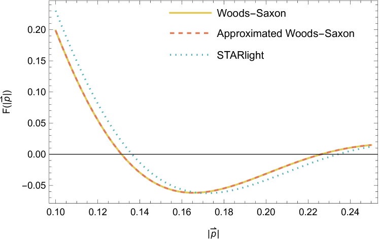
Figure 2: The Woods-Saxon form factor, the form factor adopted by this work, and the form factor in STARlight MC generator of Pb, where $R_{\mathrm{WS}}=6.62$ fm, and $d=0.546$ fm. Too see the differences between the form factors more clearly, we “zoom in” by plotting in a particular region.

The comparison of the total cross sections computed from the two form factors will also be presented later.

Based on the above results, we present the numerical analysis herein, for the Au Au collisions at RHIC and Pb Pb collisions at LHC. The nucleus radii are $R_{\mathrm{WS}}=6.38$ fm for ${}^{197}\mathrm{Au}$ and $R_{\mathrm{WS}}=6.62$ fm for ${}^{207}\mathrm{Pb}$, while the corresponding skin depths are $d=0.535$ fm for ${}^{197}\mathrm{Au}$ and $d=0.546$ fm for ${}^{207}\mathrm{Pb}$ DeVries:1987atn . As discussed earlier, one has $h_{1}^{\perp\gamma}(x,\boldsymbol{k}_{T})\simeq f_{1}(x,\boldsymbol{k}_{T})$, i.e., all photons are linearly polarized. The case that photons are partially polarized will be discussed later.

To delve into the differential cross section dependence on $\sqrt{s}$, we fix $y=0$. The resulting plot illustrates the differential cross section versus transverse momentum $q_{T}$ of pTM. We consider three distinct center-of-mass energies: $\sqrt{s}=100$, $200$, and $300$ GeV of Au Au collisions, which are around the RHIC collision energy $\sqrt{s}=200$ GeV per nucleus pair. The graphical representation is depicted in Fig. 3. Integrating over the rapidity $y$ one can have the $y$-integrated differential cross section $d\sigma/dq_{T}^{2}$, which is shown in Fig. 4. One can find that the differential cross section increases with the rising of $\sqrt{s}$, which is because that the photon density increases when $x$ goes smaller.

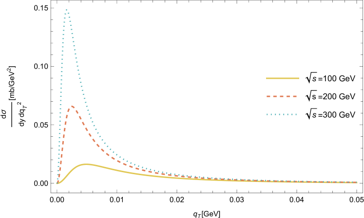
Figure 3: The differential cross section as a function of the pTM transverse momentum $q_{T}$ in Au Au collisions. We take the nucleus collision energy $\sqrt{s}=100,200,300$ GeV that are near the RHIC energy. The differential cross section exhibits an increase with the rising values of $\sqrt{s}$.

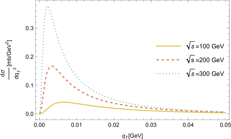
Figure 4: The $y$-integrated differential cross section as a function of $q_{T}$ with $\sqrt{s}=100,200,300$ GeV in Au Au collisions, where $y$ is the rapidity of pTM.

To see how the produced pTM is distributed with its rapidity, we integrate over $q_{T}$ and get the $q_{T}$-integrated differential cross section $d\sigma/dy$ as a function of the rapidity of pTM, which is presented in Fig. 5 for Au Au collisions and Fig. 6 for the Pb Pb collisions. Once more, we let $\sqrt{s}=100,200,300$ GeV for Au Au mode, and take $\sqrt{s}=2.76,5.02$ TeV for Pb Pb mode which corresponds to the center-of-mass energy per nucleus pair at the LHC. One can find that the rapidity of pTM at the RHIC is around $|y|\lesssim 5$, while $|y|\lesssim 8$ at the LHC.

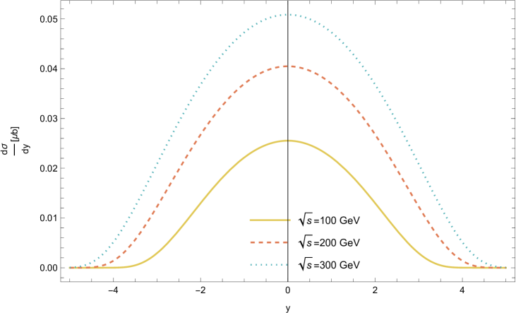
Figure 5: The $q_{T}$ integrated differential cross section $d\sigma/dy$ as a function of $y$ in Au Au collisions, where $\sqrt{s}=100,200,300$ GeV.

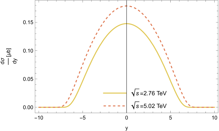
Figure 6: The $q_{T}$ integrated differential cross section $d\sigma/dy$ as a function of $y$ in Pb Pb collisions, where $\sqrt{s}=2.76$ and $5.02$ TeV.

To see how the polarization of photon affects the production of pTM, we introduce the degree of polarization $r$, which is defined as the ratio of the linearly polarized and unpolarized photon distributions, i.e., $r\equiv{h_{1}^{\perp\gamma}(x,\boldsymbol{k}_{T})}/{f_{1}^{\gamma}(x,\boldsymbol{k}_{T})}$. $r$ is generally a function, but for the sake of simplicity, we assume $r$ is a number and present the differential cross sections with $r=0,1/2,1$ in Fig. 7. When $r=0$, there is no linearly polarized photon; while for $r=1$, all of the photons are linearly polarized. One can find that the linearly polarized photons strongly effect the transverse momentum dependence in the small $q_{T}$ region, while for larger $q_{T}$ the differential cross section is not affected. It is interesting to figure out that, the differential cross section for fully linearly polarized photons decreases to zero when $q_{T}\to 0$, and the differential cross section approaches the maximum value around several MeV. It may provide a guide for searching the pTM in future experiments.

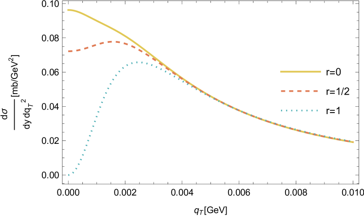
Figure 7: The differential cross section computed with $r=0$, $r=1/2$ and $r=1$, in Au Au collisions, where $r$ is the degree of photon polarization.

Integrating out $y$ and $q_{T}$ leads to the total cross section. We plot the total cross sections as the functions of $\sqrt{s}$ for both Au Au and Pb Pb collisions, which is shown in Fig. 8. Again, one can conclude that the total cross section increases when $\sqrt{s}$ increases. We list the total cross sections in Table 1. The cross sections of pTM production reported in Ginzburg:1998df are 0.15 $\mu$b for gold-gold mode at RHIC, and 1.35 $\mu$b for lead-lead collisions at LHC. Our results in Table 1 are larger, but in agreement with their results in magnitude. As a co-product of this analysis, the cross sections for the production of para-positronium (pPM) and para-true tauonium (pTT) are also presented in Table 1.

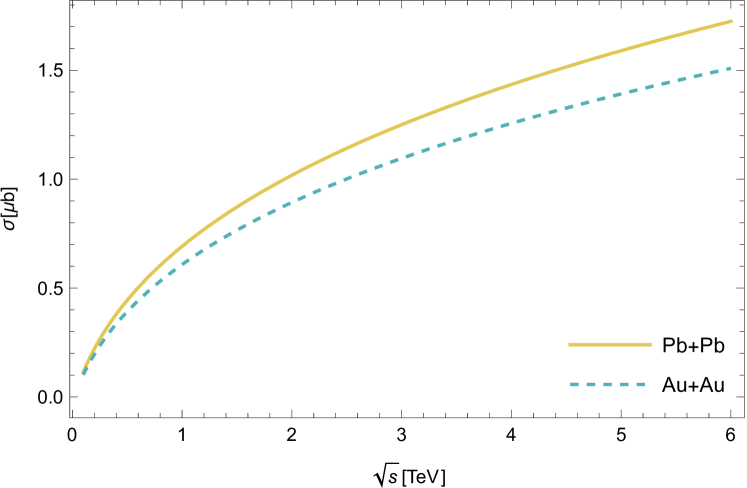
Figure 8: The total cross sections of pTM production in Au Au and Pb Pb collisions.

$\sqrt{s}$ (TeV)	0.2 (Au Au)	2.76 (Pb Pb)	5.02 (Pb Pb)
pTM cross section ($\mu$b)	0.20	1.20	1.59
pPM cross section ($\mu$b)	$1.36\times 10^{5}$	$5.85\times 10^{5}$	$4.01\times 10^{6}$
pTT cross section ($\mu$b)	$9.68\times 10^{-6}$	$6.55\times 10^{-4}$	$1.08\times 10^{-3}$

Table 1: The total cross sections of pTM production in two gamma fusion in Au Au and Pb Pb collisions. In the second row we list the cross sections of para-positronium production; while in the third row we list the cross sections for para-true tauonium.

In Figure 9, we explore the effects of different choices of nuclei form factors on the total cross sections. It indicates that the result calculated with the form factor in Eq. (12) matches well with one with the form factor adopted by STARlight, especially when $\sqrt{s}$ is not too large; when $\sqrt{s}$ is large, there may be visible differences between the two cross sections.

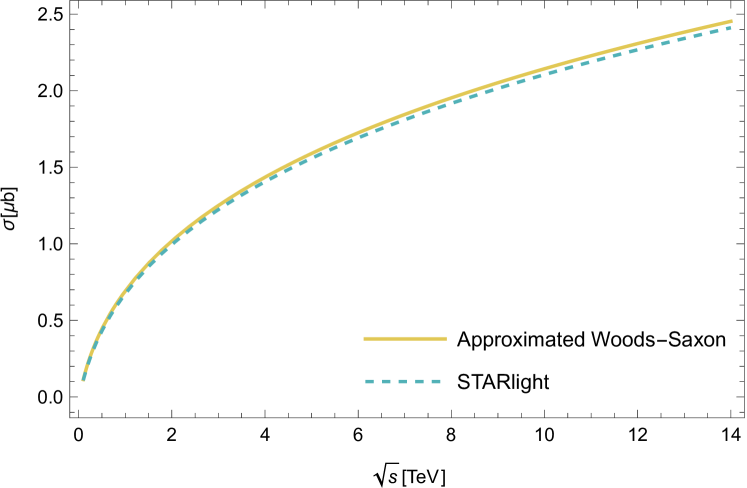
Figure 9: The total cross section of pTM production in Pb Pb collisions, computed with the form factor in Eq. 12 and the one from STARlight MC generator.

It is also intriguing to explore the average transverse momentum of pTM. We define the average transverse momentum as

$$\langle q_{T}\rangle\equiv\frac{\int dydq_{T}^{2}q_{T}\frac{d\sigma}{dydq_{T}^{2}}}{\int dydq_{T}^{2}\frac{d\sigma}{dydq_{T}^{2}}}.$$ (15)

With the differential cross sections calculated above, one can compute the numerical results of $\langle q_{T}\rangle$, which is plotted in Fig. 10. We take the Au Au collisions as an example. At the RHIC energy $\sqrt{s}=200$ GeV, $\langle q_{T}\rangle\simeq 1.4$ MeV. One can find that the average transverse momentum decreases when $\sqrt{s}$ increases. We plot $\langle q_{T}\rangle$ for both $r=0$ and $r=1$ cases, and find that the two curves coincides. Therefore, although the linearly polarized photons modify the shape of $q_{T}$ distribution, the average value $\langle q_{T}\rangle$ is not affected by the polarization.

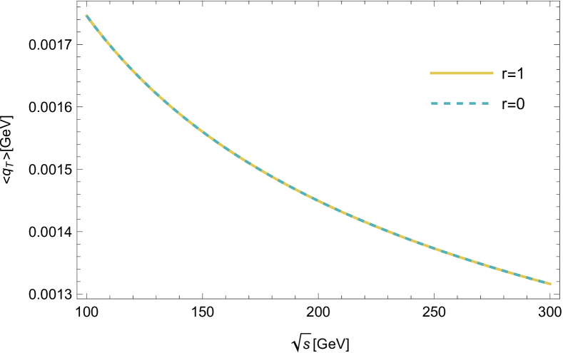
Figure 10: The average transverse momentum $\langle q_{T}\rangle$ as the function of $\sqrt{s}$ in Au Au collisions, computed in the case of $r=1$ and $r=0$, where $r$ is the degree of polarization.

To summarize, we study the para-true muonium production with photon-photon fusions in ultra-peripheral heavy ion collisions. The transverse distribution of para-true muonium is taken into explored, and to archive this purpose after taking the linearly polarized photon distribution into account. Our results indicate that the differential cross section of para-true muonium production in the small $q_{T}$ region is affected by the linearly polarized photons in nuclei significantly, and exhibits a maximum when $q_{T}$ is around several to 10 MeV at RHIC and LHC. The total cross section is also computed, indicating that significantly considerable amounts of para-true muonium should be produced. Our work can also be extend to the ortho-true muonium production in the UPC.

References

- (1) M. Deutsch, Phys. Rev. 82, 455-456 (1951) doi:10.1103/PhysRev.82.455
- (2) V. W. Hughes, D. W. McColm, K. Ziock and R. Prepost, Phys. Rev. Lett. 5, 63-65 (1960) doi:10.1103/PhysRevLett.5.63
- (3) R. Coombes, R. Flexer, A. Hall, R. Kennelly, J. Kirkby, R. Piccioni, D. Porat, M. Schwartz, R. Spitzer and J. Toraskar, et al. Phys. Rev. Lett. 37, 249-252 (1976) doi:10.1103/PhysRevLett.37.249
- (4) D. B. Cassidy, A. P. Mills, Nature 449, 195 C197 (2007).
- (5) R. E. Marshak and H. A. Bethe, Phys. Rev. 72, 506-509 (1947) doi:10.1103/PhysRev.72.506
- (6) C. M. G. Lattes, H. Muirhead, G. P. S. Occhialini and C. F. Powell, Nature 159, 694-697 (1947) doi:10.1038/159694a0
- (7) C. M. G. Lattes, G. P. S. Occhialini and C. F. Powell, Nature 160, 453-456 (1947) doi:10.1038/160453a0
- (8) C. M. G. Lattes, G. P. S. Occhialini and C. F. Powell, Nature 160, 486-492 (1947) doi:10.1038/160486a0
- (9) D. Tucker-Smith and I. Yavin, Phys. Rev. D 83, 101702 (2011) doi:10.1103/PhysRevD.83.101702 [arXiv:1011.4922 [hep-ph]].
- (10) J. Jaeckel and S. Roy, Phys. Rev. D 82, 125020 (2010) doi:10.1103/PhysRevD.82.125020 [arXiv:1008.3536 [hep-ph]].
- (11) J. Kopp, L. Michaels and J. Smirnov, JCAP 04, 022 (2014) doi:10.1088/1475-7516/2014/04/022 [arXiv:1401.6457 [hep-ph]].
- (12) P. Agrawal, M. Bauer, J. Beacham, A. Berlin, A. Boyarsky, S. Cebrian, X. Cid-Vidal, D. d’Enterria, A. De Roeck and M. Drewes, et al. Eur. Phys. J. C 81, no.11, 1015 (2021) doi:10.1140/epjc/s10052-021-09703-7 [arXiv:2102.12143 [hep-ph]].
- (13) S. Bilenikii, N. van Hieu, L. Nemenov, and F. Tkebuchava, Sov. J. Nucl. Phys. 10, 469 (1969).
- (14) V. W. Hughes and B. Maglic, Bull. Am. Phys. Soc. 16, 65 (1971).
- (15) J. Malenfant, Phys. Rev. D 36, 863-877 (1987) doi:10.1103/PhysRevD.36.863
- (16) U. D. Jentschura, V. G. Ivanov, G. Soff and S. G. Karshenboim, Phys. Lett. B 424, 397-404 (1998) doi:10.1016/S0370-2693(98)00206-8 [arXiv:hep-ph/9706401 [hep-ph]].
- (17) R. L. Workman et al. [Particle Data Group], PTEP 2022, 083C01 (2022) doi:10.1093/ptep/ptac097
- (18) R. Francener, V. P. Goncalves and B. D. Moreira, Eur. Phys. J. A 58, no.2, 35 (2022) doi:10.1140/epja/s10050-022-00689-8 [arXiv:2110.03466 [hep-ph]].
- (19) N. Arteaga-Romero, C. Carimalo and V. G. Serbo, Phys. Rev. A 62, 032501 (2000) doi:10.1103/PhysRevA.62.032501 [arXiv:hep-ph/0001278 [hep-ph]].
- (20) P. A. Krachkov and A. I. Milstein, Nucl. Phys. A 971, 71-82 (2018) doi:10.1016/j.nuclphysa.2018.01.013 [arXiv:1712.09770 [hep-ph]].
- (21) A. Banburski and P. Schuster, Phys. Rev. D 86, 093007 (2012) doi:10.1103/PhysRevD.86.093007 [arXiv:1206.3961 [hep-ph]].
- (22) I. F. Ginzburg, U. D. Jentschura, S. G. Karshenboim, F. Krauss, V. G. Serbo and G. Soff, Phys. Rev. C 58, 3565-3573 (1998) doi:10.1103/PhysRevC.58.3565 [arXiv:hep-ph/9805375 [hep-ph]].
- (23) Y. Chen and P. Zhuang, [arXiv:1204.4389 [hep-ph]].
- (24) G. M. Yu and Y. D. Li, Chin. Phys. Lett. 30, 011201 (2013) doi:10.1088/0256-307X/30/1/011201
- (25) C. Azevedo, V. P. Gonçalves and B. D. Moreira, Phys. Rev. C 101, no.2, 024914 (2020) doi:10.1103/PhysRevC.101.024914 [arXiv:1911.10861 [hep-ph]].
- (26) G. Yu, Z. Zhao, Y. Cai, Q. Gao, Q. Hu and H. Yang, [arXiv:2209.11439 [hep-ph]].
- (27) R. Francener, V. P. Goncalves and B. D. Moreira, Eur. Phys. J. A 58, no.2, 35 (2022) doi:10.1140/epja/s10050-022-00689-8 [arXiv:2110.03466 [hep-ph]].
- (28) L. Nemenov, Yad. Fiz. 15, 1047 (1972) [Sov. J. Nucl. Phys. 15, 582 (1972)]; G. A. Kozlov, Yad. Fiz. 48, 265 (1988) [Sov. J. Nucl. Phys. 48, 167 (1988)].
- (29) X. Cid Vidal, P. Ilten, J. Plews, B. Shuve and Y. Soreq, Phys. Rev. D 100, no.5, 053003 (2019) doi:10.1103/PhysRevD.100.053003 [arXiv:1904.08458 [hep-ph]].
- (30) J. W. Moffat, Phys. Rev. Lett. 35, 1605 (1975) doi:10.1103/PhysRevLett.35.1605
- (31) S. J. Brodsky and R. F. Lebed, Phys. Rev. Lett. 102, 213401 (2009) doi:10.1103/PhysRevLett.102.213401 [arXiv:0904.2225 [hep-ph]].
- (32) R. Gargiulo, E. Di Meco, D. Paesani, S. Palmisano, E. Diociaiuti and I. Sarra, [arXiv:2309.11683 [hep-ph]].
- (33) Y. Ji and H. Lamm, Phys. Rev. D 98, no.5, 053008 (2018) doi:10.1103/PhysRevD.98.053008 [arXiv:1706.04986 [hep-ph]].
- (34) A. Sommerfeld, Atombau und Spektrallinien (Vieweg, Braunschweig, 1939), Vol. II; A. D. Sakharov, Sov. Phys. JETP 18, 631 (1948); J. Schwinger, Particles, Sources, and Fields (Perseus, New York, 1998), Vol. 2.
- (35) J. D. Bjorken, Lect. Notes Phys. 56, 93 (1976) SLAC-PUB-1756.
- (36) F. A. Harris [BES], Int. J. Mod. Phys. A 24, 377-384 (2009) doi:10.1142/S0217751X09043705 [arXiv:0808.3163 [physics.ins-det]].
- (37) T. Abe et al. [Belle-II], [arXiv:1011.0352 [physics.ins-det]].
- (38) A. J. Baltz, G. Baur, D. d’Enterria, L. Frankfurt, F. Gelis, V. Guzey, K. Hencken, Y. Kharlov, M. Klasen and S. R. Klein, et al. Phys. Rept. 458, 1-171 (2008) doi:10.1016/j.physrep.2007.12.001 [arXiv:0706.3356 [nucl-ex]].
- (39) M. Aaboud et al. [ATLAS], Nature Phys. 13, no.9, 852-858 (2017) doi:10.1038/nphys4208 [arXiv:1702.01625 [hep-ex]].
- (40) E. Fermi, Z. Phys. 29, 315-327 (1924) doi:10.1007/BF03184853
- (41) C. F. von Weizsacker, Z. Phys. 88, 612-625 (1934) doi:10.1007/BF01333110
- (42) E. J. Williams, Kong. Dan. Vid. Sel. Mat. Fys. Med. 13N4, no.4, 1-50 (1935)
- (43) C. Li, J. Zhou and Y. J. Zhou, Phys. Lett. B 795, 576-580 (2019) doi:10.1016/j.physletb.2019.07.005 [arXiv:1903.10084 [hep-ph]].
- (44) J. Adam et al. [STAR], Phys. Rev. Lett. 127, no.5, 052302 (2021) doi:10.1103/PhysRevLett.127.052302 [arXiv:1910.12400 [nucl-ex]].
- (45) D. Boer and C. Pisano, Phys. Rev. D 86, 094007 (2012) doi:10.1103/PhysRevD.86.094007 [arXiv:1208.3642 [hep-ph]].
- (46) J. P. Ma, J. X. Wang and S. Zhao, Phys. Rev. D 88, no.1, 014027 (2013) doi:10.1103/PhysRevD.88.014027 [arXiv:1211.7144 [hep-ph]].
- (47) R. D. Woods and D. S. Saxon, Phys. Rev. 95, 577-578 (1954) doi:10.1103/PhysRev.95.577
- (48) M. Y. Şengül, M. C. Güçlü, Ö. Mercan and N. G. Karakuş, Eur. Phys. J. C 76, no.8, 428 (2016) doi:10.1140/epjc/s10052-016-4269-4 [arXiv:1508.07051 [hep-ph]].
- (49) S. Klein and J. Nystrand, Phys. Rev. C 60, 014903 (1999) doi:10.1103/PhysRevC.60.014903 [arXiv:hep-ph/9902259 [hep-ph]].
- (50) S. R. Klein, J. Nystrand, J. Seger, Y. Gorbunov and J. Butterworth, Comput. Phys. Commun. 212, 258-268 (2017) doi:10.1016/j.cpc.2016.10.016 [arXiv:1607.03838 [hep-ph]].
- (51) H. De Vries, C. W. De Jager and C. De Vries, Atom. Data Nucl. Data Tabl. 36, 495-536 (1987) doi:10.1016/0092-640X(87)90013-1