Solving the Scattering Problem for Open Wave-Guides, III:
Radiation Conditions and Uniqueness

Abstract

This paper continues the analysis of the scattering problem for a network of open wave-guides started in [7, 8]. In this part we present explicit, physically motivated radiation conditions that ensure uniqueness of the solution to the scattering problem. These conditions stem from a 2000 paper of Vasy on 3-body Schrödinger operators, see [21]; we also discuss closely related conditions from a 1994 paper of Isozaki  [11]. Vasy’s paper also proves the existence of the limiting absorption resolvents, and that the limiting solutions satisfy the radiation conditions. The statements of these results require a calculus of pseudodifferential operators, called the 3-body scattering calculus, which is briefly introduced here. We show that the solutions to the model problem obtained in [7] satisfy these radiation conditions, which makes it possible to prove uniqueness, and therefore existence, for the system of Fredholm integral equations introduced in that paper.

1 Introduction

Many opto-electronic and photonic devices are modeled as open wave-guides. In such devices there are channels defined by spatial variations in the electrical permittivity, but the channels are unclad, so the electromagnetic waves are not confined to the channel. Such physical systems are described by Maxwell’s equations with spatially dependent permittivity. In this paper we consider a simpler scalar model, wherein the permittivity $\epsilon(x)$ is a positive real-valued function, constant outside the set $\Omega=\bigcup_{\alpha\in\mathcal{A}}T_{\alpha}\cup\Omega_{0}.$ Here $\Omega_{0}$ is a compact set, and each $T_{\alpha}$ is a ‘tube’ unbounded in one direction. Fix a set of points $\{v_{\alpha}:\>\alpha\in\mathcal{A}\}$ on the unit sphere $S^{d-1}$, for some positive constants, $d_{\alpha},R_{\alpha}$, let

$$T_{\alpha}=\{x:\>|P_{\alpha}(x)|<d_{\alpha},\,\langle x,v_{\alpha}\rangle>R_{\alpha}\}.$$ (1)

Here

$$P_{\alpha}(x)=x-\langle x,v_{\alpha}\rangle v_{\alpha}$$ (2)

is the projection onto the hyperplane $\{w:\langle w,v_{\alpha}\rangle=0\}$. We assume here that $\epsilon\in\mathcal{C}^{\infty}(\mathbb{R}^{d}),$ and for each $\alpha\in\mathcal{A}$, $\epsilon\upharpoonright_{T_{\alpha}}$ depends only on $P_{\alpha}(x)$ for $\langle x,v_{\alpha}\rangle>R^{\prime}_{\alpha}>R_{\alpha}$, see Figure 2.

To focus on the key ideas, assume that $\epsilon=\epsilon_{1}\in\mathbb{R}^{+}$ outside of $\Omega$. We consider the time harmonic case, with time dependence $e^{-ift},$ and thus seek solutions to

$$(\Delta+q(x)+k^{2})u=0,$$ (3)

where

$$q(x)=(\epsilon(x)-\epsilon_{1})f^{2}\text{ and }k^{2}=\epsilon_{1}f^{2}.$$ (4)

In time–independent scattering theory, one imagines that there is an ‘incoming’ field $u^{\operatorname{in}}(x),$ which is either a wave-guide mode (see Section 3) for one of the channels, or a free-space wave packet (see Section 6 of [7]). We then look for an ‘outgoing’ solution to

$$(\Delta+q(x)+k^{2})u^{\operatorname{out}}=-(\Delta+q(x)+k^{2})u^{\operatorname{in}},$$ (5)

so that $u^{\operatorname{tot}}=u^{\operatorname{in}}+u^{\operatorname{out}}$ represents the total field that results from the incoming field scattering off of the wave-guide structure.

There are many papers in the Applied Math and Physics literature that consider such problems; see [1, 2, 3, 4] in the Applied Math literature, and [16, 12] and the references therein for the Mathematical Physics literature. What these various papers do not provide, however, are rigorous, physically motivated definitions of the concepts ‘incoming’ and ‘outgoing’ for the full $d$-dimensional problem. They also do not prove a uniqueness result for this scattering problem, which is a central component of a complete theory. The fact that the potential $q(x)$ does not vanish at infinity is what makes this challenging, and not covered by the more standard ‘two-body’ scattering literature. In particular, the classical Sommerfeld radiation conditions must be reformulated to give new and tractable criteria for uniqueness in this setting. To the best of our knowledge, none of the approaches in the literature for solving this problem are amenable to a numerical realization, which provides an accurate representation of the radiation field outside of the channels.

This latter issue is addressed in [7, 8] for the simple model problem of two semi-infinite rectangular channels in $\mathbb{R}^{2}$ that meet along a common perpendicular line, with a piecewise constant potential, see Figure 1. These papers reformulate the scattering problem as a transmission problem, which is solved using an integral equation approach. This representation also yields precise asymptotics for the solutions. In the present paper we present radiation conditions that imply uniqueness and are satisfied by the ‘limiting absorption solutions.’ We assume here, to conform with earlier literature, that the potential is smooth. The integral equation method from [7, 8] can easily be adapted to handle smooth potentials; on the other hand, by a modification of the techniques used here, such as those in [17], it should be possible to extend the results of this paper to the piecewise constant case.

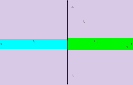
Figure 1: Two dielectric channels in $\mathbb{R}^{2}$ meeting along a straight interface.

In fact, radiation conditions for similar multi-channel scattering problems were treated in the mathematical physics literature as far back as the mid-1990’s. In [11] H. Isozaki provided a solution to this problem in the setting of $N$-body Schrödinger potentials. The assumptions he makes on the potential exclude the ones considered here. Nonetheless his results apply to open wave-guides as shown by a different analysis of the problem due to Vasy, culminating in the paper [21]. Vasy uses the tools of geometric microlocal analysis, significantly refining a method introduced by Melrose in [13] to study scattering theory for potentials with sufficient decay. The key new idea proposed by Melrose is that the oscillations ‘at infinity’ and decay of solutions to $(\Delta+q(x)+k^{2})u=f\in\mathcal{S}(\mathbb{R}^{d})$ can be encoded in a geometric notion called the scattering wave-front set. He shows that this set is strongly constrained by the asymptotic behavior of the operator itself. Vasy’s work generalizes this approach considerably, incorporating potentials that do not decay along certain (possibly higher dimensional) channels.

The principal goal of the present paper is to present the Isozaki/Vasy radiation conditions in a form usable for open wave-guides. Since the channels are concentrated along rays (rather than higher dimensional subspaces), many details in [11, 13, 21] simplify. The work of Melrose and Vasy also gives a precise explanation for the nature of the radiation conditions, and explains why Isozaki’s conditions suffice. We give a brief accounting of their work, but refer to those papers for the detailed technical arguments. We also apply these conditions to the solutions obtained in [7, 8], thus showing that they are indeed outgoing and agree with the limiting absorption solutions, whose existence is demonstrated in [21].

One important aspect of all of this is that radiation conditions are essentially local at infinity. The following language makes this precise. Denote by $\overline{\mathbb{R}^{d}}$ the radial compactification of $\mathbb{R}^{d},$ which adds a boundary point for each direction. Altogether we add a unit sphere $S^{d-1}$ consisting of all such asymptotic directions, and thus $\overline{\mathbb{R}^{d}}$ is diffeomorphic to the closed unit ball. It is convenient to start with polar coordinates, $r=|x|\geq 0$, $\omega=x/|x|\in S^{d-1}.$ Setting $\rho=1/r$ gives coordinates, $(\rho,\omega),$ near $\partial\overline{\mathbb{R}^{d}}$ with

$$\partial\overline{\mathbb{R}^{d}}=\{\rho=0,\,\omega\in S^{d-1}\}.$$ (6)

The points $\mathcal{C}=\{v_{\alpha}:\>\alpha\in\mathcal{A}\}\subset\partial\overline{\mathbb{R}^{d}},$ corresponding to the directions of the channels, are called the channel ends, and the complement $\mathcal{C}^{c}=S^{d-1}\setminus\mathcal{C}$ is called the free boundary. We localize a function near a point $\omega_{0}\in\partial\overline{\mathbb{R}^{d}}$ by multiplying by a cut-off function $\Psi\in\mathcal{C}^{\infty}(\overline{\mathbb{R}^{d}})$ which equals $1$ near $\omega_{0}$ and which vanishes outside a small neighborhood of that point. For example, we can use smooth, ‘conical cut-offs’

$$\Psi_{\omega_{0},\delta}(x)=\begin{cases}&1\text{ for }\left|\frac{x}{|x|}-\omega\right|<\delta,|x|>C+1,\\ &\phantom{=}\\ &0\text{ for }\left|\frac{x}{|x|}-\omega\right|>2\delta,|x|<C,\end{cases}$$ (7)

for any $C>0$; the parameter $\delta>0$ measures the aperture of the conical neighborhood.

Isozaki defines the notion of incoming and outgoing solutions using a certain class of admissible operators $\mathcal{R}_{\pm}(\epsilon)$: a solution $u$ is incoming ($+$), resp. outgoing ($-$), near $\omega_{0},$ if there there exist $P_{\pm}\in\mathcal{R}_{\pm}(\epsilon)$ and numbers $\delta,\delta^{\prime}>0$ such that for some $\eta>0$,

$$\rho^{\frac{1}{2}-\eta}\Psi_{\omega_{0},\delta^{\prime}}P_{\pm}[\Psi_{\omega_{0},\delta}u]\in L^{2}(\mathbb{R}^{d}).$$ (8)

Notice that $\rho^{\frac{1}{2}-\eta}f\in L^{2}$ means that (at least on average) $f$ decays faster than $r^{\frac{1-d}{2}}$. The operators in $\mathcal{R}_{\pm}(\epsilon)$ are essentially pseudodifferential operators, which we describe below. Somewhat mysteriously, they do not depend, in an essential way, on the background wave number, $k^{2}.$ The Melrose/Vasy theory provides an explanation for this fact. In the sequel, the operation

$$u\longmapsto\mathcal{F}(\Psi_{\omega_{0},\delta}u)$$ (9)

is often referred to as a conical Fourier transform.

It is clear from Isozaki’s treatment that the radiation conditions reflect the singularities of the conic Fourier transforms of the solution $u,$ that is $\mathcal{F}[\Psi_{\omega,\delta}u](\xi).$ This connection is made explicit in the classical setting of potentials vanishing at infinity in [13] and leads directly to what Melrose calls the scattering wave-front set, as mentioned above. Vasy [21] extends this notion to a class of non-compactly supported potentials that includes open wave-guide potentials. Isozaki’s admissible operators are subsumed in a larger and more flexible class of pseudodifferential operators, which constitute the 3-body scattering calculus. The ensuing microlocal treatment explains many aspects of the radiation conditions in terms of propagation phenomena similar to those that arise in solutions of hyperbolic equations. Vasy also proves that a solution to $(\Delta+q+k^{2})u=f\in\mathcal{S}(\mathbb{R}^{d}),$ which is either incoming or outgoing, in this extended sense, is unique. This is used to show the existence of the limiting absorption resolvents $(\Delta+q+k^{2}\pm i0)^{-1}=\lim_{\sigma\to 0^{+}}(\Delta+q+k^{2}\pm i\sigma)^{-1}$, which produce these unique incoming ($-$) and outgoing ($+$) solutions.

We remark here that both Isozaki and Vasy work in a setting that includes more general $N$-body potentials in Euclidean space. One key new feature, when $N>3$, is that the channels (which are concentrated along subspaces and not just lines) may intersect at infinity; this does not occur when $N=3$. Our geometric assumptions about channels ensure that this does not happen, and for this reason we may employ tools adapted to the setting of 3-body potentials. In the $N$-body Schrödinger equation literature the channels are at least 2 dimensional and so they meet $\partial\overline{\mathbb{R}^{d}}$ in a positive dimensional set. This precludes the use of conic localization near the ends of the channels, which is a significant simplification in the wave-guide case.

We begin in Section 2 by recalling the classically understood behavior of solutions to $(\Delta+q(x)+k^{2})u\in\mathcal{S}$ where the potential $q(x)$ decays at infinity. In Section 3 we give a more detailed description of the wave-guide models we consider here, as well as the definition of wave-guide modes. In Section 4 we consider the two versions of the radiation conditions for the open wave-guide problem. Isozaki’s condition requires less background to explain, but to present Vasy’s conditions, we must describe both Melrose’s scattering calculus and Vasy’s 3-body scattering calculus. In Section 5 we prove that the solutions obtained in [7, 8] are outgoing in the sense of Isozaki/Vasy. These calculations illustrate our assertion that Vasy’s conditions are more flexible and easier to check in specific examples. We finally prove the missing uniqueness theorem for the Fredholm integral equations of second kind introduced in [7], which thereby completes the proof of the existence of solutions to the transmission problem.

Additional results are given in two appendices. In the first we show, by direct computation, that a classically outgoing solution satisfies Isozaki’s form of the radiation condition. In the second we show that the channel-to-channel scattering coefficients are well defined for an open wave-guide.

Acknowledgments

The authors wish to thank Andras Vasy for very helpful conversations at various stages in the exploration of this problem, and for his careful reading and comments on an earlier version of this paper.

2 Channel-free scattering

Before turning to the main topic of interest here, we briefly review some classical facts about scattering in Euclidean backgrounds. We consider both the ‘free’ case, i.e. for the Helmholtz equation $(\Delta+k^{2})u=0$ in $\mathbb{R}^{d}$, and then a few generalizations to the equation $(\Delta+q(x)+k^{2})u=0$ where $q(x)$ is a smooth, short range potential, i.e. vanishing at infinity at least as fast as $|x|^{-1-\epsilon}$ for some $\epsilon>0$. All of this material is classical and well-known.

Consider first the space of solutions to $(\Delta+k^{2})u=0$ in all of Euclidean space. There are two key building blocks for all other solutions: the first is the class of plane wave solutions:

$$u_{k,\omega_{0}}(x)=e^{ikx\cdot\omega_{0}}$$

where $\omega_{0}\in S^{d-1}$ is fixed. While these seem quite simple, they are actually singular in one respect, as we explain below, in that they they do not decay at infinity. There is another basic set of solutions; in $\mathbb{R}^{2}$ these are the functions

$$Z_{\ell}(kr)e^{\pm i\ell\phi},\quad k,\ell\in\mathbb{N}_{0},$$

with $Z_{\ell}$ any Bessel function of order $\ell.$

These have analogues in dimensions $d>2,$ where the factors $e^{\pm i\ell\phi}$ are replaced by spherical harmonics: For any solution to $\Delta_{S^{d-1}}Y=-\lambda^{2}Y,$ there are solutions to the Helmholtz equation of the form $r^{\frac{2-d}{2}}Z_{\nu}(kr)Y(\omega)$. Here $Z_{\nu}(r)$ is any Bessel function of order $\nu={\pm\sqrt{\lambda^{2}+\left(\frac{d-2}{2}\right)^{2}}}.$ As the eigenvalues on $S^{d-1}$ are $\lambda^{2}=\ell(d-2+\ell)$, $\ell\in\mathbb{N}_{0}$, the degrees $\nu_{\ell}=\pm\left(\ell+\frac{d-2}{2}\right)$. Using standard asymptotics of Bessel functions, we have that the globally smooth solutions satisfy

$$v_{k,\ell}^{\pm}(r,\phi)\overset{d}{=}J_{\ell}(kr)e^{\pm i\ell\phi}\sim\frac{e^{\pm i\ell\phi}}{\sqrt{r}}(a_{0}^{+}e^{ikr}+a_{0}^{-}e^{-ikr})$$

for some constants $a_{0}^{\pm}.$

There appears to be a stark difference between these two classes of solutions: the $u_{k,\omega_{0}}$ are bounded but do not decay, and they oscillate, but with ‘radial frequency’ reaching a maximum only in the directions $\pm\omega_{0}$. By contrast, the $v_{k,\ell}^{\pm}$ decay slowly but at a fixed rate, and oscillate uniformly in the radial direction at frequencies $\pm k.$ These solutions are closely related, by virtue of the classical formula

$$J_{\ell}(kr)=\int_{S^{1}}\left[A_{\ell}^{+}(\omega)e^{ik\omega\cdot x}+A_{\ell}^{-}(\omega)e^{-ik\omega\cdot x}\right]\,dV_{\omega},$$

for certain smooth functions $A_{\ell}^{\pm}(\omega)$ on the circle. This formula is basically equivalent to the classical integral definition of the $J$-Bessel function:

$$J_{\ell}(r)=\frac{i^{-\ell}}{\pi}\int_{0}^{\pi}e^{ir\cos\phi}\cos(\ell\phi)\,d\phi.$$

These smooth, decaying solutions are simply averages over all directions of the plane wave solutions, with suitably chosen amplitudes.

Motivated by these two examples, we quote a result about general solutions to $(\Delta+k^{2})u=0$ in any external region $|x|\geq R$. Namely, any such solution admits an asymptotic expansion of the form

$$u(x)\sim r^{\frac{1-d}{2}}\left[e^{ikr}\sum_{j=0}^{\infty}a_{j}^{+}(\omega)r^{-j}+e^{-ikr}\sum_{j=0}^{\infty}a_{j}^{-}(\omega)r^{-j}\right].$$ (10)

The meaning of this asymptotic expansion is unexpectedly subtle in that the coefficients $a_{j}^{\pm}(\omega)$ are, in general, only distributions on the sphere. Thus to make sense of this, we must average, i.e., integrate against a smooth test function in $\omega$. Thus the actual meaning of (10) is that if $\chi(\omega)\in\mathcal{C}^{\infty}(S^{d-1})$ is arbitrary, then

$$\begin{split}&\int_{S^{d-1}}u(r\omega)\chi(\omega)\,dV_{\omega}\\ &\qquad\qquad\sim r^{\frac{1-d}{2}}\left[e^{ikr}\sum_{j=0}^{\infty}\langle a_{j}^{+},\chi\rangle r^{-j}+e^{-ikr}\sum_{j=0}^{\infty}\langle a_{j}^{-},\chi\rangle r^{-j}\right].\end{split}$$ (11)

As a function of the radial variable $r$ alone, this is an asymptotic expansion, in the traditional sense, for a function of one variable. The existence of such expansions, when the leading coefficients are smooth functions on $S^{d-1},$ is sketched in [14, Section 1.3] using stationary phase. The existence of a leading distributional term in general is also noted there; the complete distributional expansion can be obtained by an iterative argument using the Mellin transform in the radial variable.

The functions $v_{k,\ell}$ satisfy these asymptotic conditions in the usual strong sense since the amplitude functions $a^{\pm}_{0}e^{\pm il\phi}$ are smooth. The plane wave solutions admit an expansion of this form, albeit with distributional coefficients. Writing $x=r\omega$, we have

$$e^{ikr\omega\cdot\omega_{0}}\sim c_{d}r^{\frac{1-d}{2}}[e^{ikr-i\pi/4}\delta_{\omega_{0}}(\omega)+e^{-ikr+i\pi/4}\delta_{-\omega_{0}}(\omega)].$$

To see that this holds, we apply stationary phase to get that, for any $N>0,$

$$\int_{S^{d-1}}e^{ikr\omega\cdot\omega_{0}}\chi(\omega)\,dV_{\omega}=\\ c_{d}r^{\frac{1-d}{2}}[e^{ikr-i\pi/4}\chi(\omega_{0})+e^{-ikr+i\pi/4}\chi(-\omega_{0})]+O(r^{-N}),$$ (12)

as $r\to\infty.$

Definition 1.

A formal solution $u$ to $(\Delta+k^{2})u=f$, where $f\in\mathcal{S}(\mathbb{R}^{d})$ and $u$ is a priori only assumed to be polynomially bounded (i.e., in the dual Schwartz space, $\mathcal{S}^{\prime}(\mathbb{R}^{d})$) is called outgoing if, in (10), all of the coefficients $a_{j}^{-}(\omega)$ vanish identically. In other words, a solution is said to satisfy the outgoing condition if

$$u(r\omega)\sim r^{\frac{1-d}{2}}e^{ikr}\sum_{j=0}^{\infty}r^{-j}a_{j}^{+}(\omega).$$

It is a non-trivial fact, proved in [13], that if $u$ is outgoing (and $f$ is Schwartz), then all of the coefficients $a_{j}^{+}(\omega)$ are $\mathcal{C}^{\infty}$. Granting this, then an integration by parts leads to the conclusion that if $f\equiv 0$ and $u$ is outgoing, then $u\equiv 0$. In other words, there are no non-trivial globally defined outgoing solutions. There is an analogous notion that a solution is called incoming if all of the ‘positive’ coefficients, $\{a_{j}^{+}(\omega)\},$ in its expansion vanish. Everything that we say here about outgoing solutions has a direct analogue for incoming solutions.

The explicit solutions $v_{k,\ell}$ we wrote down earlier are neither incoming nor outgoing, since both coefficients $a_{0}^{\pm}$ are non-vanishing. However, there is another solution of the Bessel equation called the Hankel function of the first kind, denoted $H_{\nu}^{(1)}$, so that $w_{k,d}(r\omega)=r^{\frac{2-d}{2}}H_{(d-2)/2}^{(1)}(kr)$ is an outgoing solution to the Helmholtz equation in $\mathbb{R}^{d}\setminus\{0\}.$ It has a singularity at $r=0$, which is in agreement with the fact that there are no globally defined outgoing solutions. This solution is used to define the outgoing fundamental solution for $(\Delta+k^{2}).$

The classical Sommerfeld condition provides a criterion to check whether a solution $u$ is outgoing without the need for an asymptotic expansion. Observe that even in the ‘best’ case where all $a_{j}^{\pm}$ are smooth, the leading terms $e^{\pm ikr}r^{(1-d)/2}$ do not lie in $L^{2}(\mathbb{R}^{d})$. However, applying the operator $\partial_{r}-ik$ to $u$ reduces the order of growth of one of these terms:

$$\left(\partial_{r}-ik\right)e^{ikr}r^{\frac{1-d}{2}}=\left(\frac{1-d}{2}\right)e^{ikr}r^{-\frac{1+d}{2}},$$

which does lie in $L^{2}(\mathbb{R}^{d})$. On the other hand, applying $\partial_{r}-ik$ to $e^{-ikr}r^{(1-d)/2}$ does not yield better decay. As the coefficients $a_{j}^{\pm}$, $j>0$, all depend linearly on $a_{0}^{\pm}$, it follows that

$$\mbox{The solution}\ u\ \mbox{is outgoing if}\ \left(\partial_{r}-ik\right)u\in L^{2}(\mathbb{R}^{d}).$$ (13)

In fact the weaker conditions

$$r^{\delta-\frac{1}{2}}(\partial_{r}-ik)u(r\omega)\in L^{2}(\mathbb{R}^{d})\text{ for a }\delta>0$$ (14)

suffice to conclude that a solution is outgoing.

Note that given any $f\in\mathcal{S}$, there exists a unique outgoing solution $u$ to $(\Delta+k^{2})u=f$. This solution is obtained by convolving with the outgoing resolvent:

$$u=\int_{\mathbb{R}^{d}}R_{k^{2}+i0}(x,\tilde{x})f(\tilde{x})\,dV_{\tilde{x}}.$$

The operator $R_{k^{2}+i0}$ is the outgoing resolvent, whose integral kernel is the radial function

$$R_{k^{2}+i0}(x,\tilde{x})=C_{d}\frac{H^{(1)}_{\frac{d-2}{2}}(k|x-\tilde{x}|)}{|x-\tilde{x}|^{\frac{d-2}{2}}}.$$ (15)

Everything we have said here has an analogue for the general Schrödinger operators

$$(H+k^{2})u:=(\Delta+q(x)+k^{2})u,$$

where $q$ is sufficiently regular and decays sufficiently rapidly at infinity. A solution to $(H+k^{2})u=f\in\mathcal{S}(\mathbb{R}^{d})$ is outgoing if it satisfies (14). We no longer have explicit solutions, but one can still prove the existence of an outgoing resolvent $R(k^{2}+i0)$, as well as the existence of expansions for solutions to $(H+k^{2})u=f$. The existence of the outgoing resolvent is called the limiting absorption principle: If $\sigma>0,$ then the resolvent operators $R(k^{2}\pm i\sigma)=(H+k^{2}\pm i\sigma)^{-1}$ are well defined as bounded operators on $L^{2}(\mathbb{R}^{d}),$ which, in fact map $\mathcal{S}(\mathbb{R}^{d})$ to itself. The limiting absorption principle states that,

$$R(k^{2}\pm i0)=\lim_{\sigma\to 0^{+}}R(k^{2}\pm i\sigma)$$ (16)

exist as bounded maps from $r^{-(\delta+\frac{1}{2})}L^{2}(\mathbb{R}^{d})$ to $r^{\delta+\frac{1}{2}}L^{2}(\mathbb{R}^{d}),$ for any $\delta>0.$ Moreover, if $w\in\mathcal{S}(\mathbb{R}^{d}),$ then

$$u_{\pm}=R(k^{2}\pm i0)w$$ (17)

is the unique outgoing ($+$), resp. incoming ($-$) solution to

$$(\Delta+q+k^{2})u_{\pm}=w.$$ (18)

These extensions are covered in [13] and [19].

3 Open Wave-Guides and Wave-Guide Modes

The main goal of this paper is to provide physically motivated, radiation conditions that imply uniqueness for open wave-guides. We first describe the mathematical model we use for an open wave-guide in $\mathbb{R}^{d}:$ imagine a collection of dielectric, non-conducting, non-magnetic, ‘pipes,’ which interact in a compact region of space, and are asymptotic to disjoint straight lines as they head off to infinity, see Figure 2. Within the pipes the permittivity is spatially dependent, whereas in the exterior region it assumes a constant positive real value. We work in the time-harmonic setting, with solutions of the form $e^{-ift}u(x)$ for an $f>0.$ If $\epsilon_{1}$ denotes the permittivity outside of the dielectric network, then $k^{2}=\epsilon_{1}f^{2}$ is the ‘free space’ wave number.

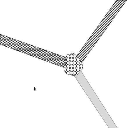
Figure 2: Three dielectric channels meeting in a compact interaction zone, $D.$

We next describe the channel regions. As in the introduction, fix a finite set of asymptotic directions $\mathcal{C}=\{v_{\alpha}:\>\alpha\in\mathcal{A}\}\subset\partial\overline{\mathbb{R}^{d}}\simeq S^{d-1}$, and for each $\alpha$, denote by $P_{\alpha}$ the orthogonal projection onto the orthocomplement of $v_{\alpha}$. Following standard conventions in $N$-body scattering theory, we write

$$x_{\alpha}=\langle x,v_{\alpha}\rangle,\ \ \mbox{and}\ \ \ x^{\alpha}=P_{\alpha}x=x-x_{\alpha}v_{\alpha}.$$ (19)

Finally, let $\epsilon_{\alpha}\in\mathcal{C}^{\infty}_{c}(\operatorname{Im}P_{\alpha})$ be a real valued function that describes the variation of permittivity within the channel for $\langle x,v_{\alpha}\rangle$ sufficiently large. At frequency $f$ we set $q_{\alpha}=f^{2}(\epsilon_{\alpha}-\epsilon_{1})$; this represents the deviation from the free space wave-number within that channel. In the central region where the channels intersect, we let $q_{0}=f^{2}(\epsilon_{0}-\epsilon_{1})\in\mathcal{C}^{\infty}_{c}(\mathbb{R}^{d})$ denote the potential which describes their interactions. Finally, choose $\psi_{+}\in\mathcal{C}^{\infty}(\mathbb{R}),$ vanishing for $t<1,$ and equals to $1$ for $t>2$. In terms of this data, the model for the open wave-guide network at frequency $f$ is given by the time-independent Schrödinger operator

$$H+k^{2}=(\Delta+q+k^{2}),$$ (20)

where

$$q(x)=q_{0}(x)+\sum_{\alpha\in\mathcal{A}}q_{\alpha}(x^{\alpha})\psi_{+}(r_{\alpha}x_{\alpha}),$$ (21)

for fixed positive constants $r_{\alpha}$. The support of $q(x)$ outside a large compact set lies in a bounded neighborhood of the collection of rays $\{rv_{\alpha}:\>r\gg 0,\,\alpha\in\mathcal{A}\}.$ These meet $\partial\overline{\mathbb{R}^{d}}=S^{d-1}$ at the points

$$\mathcal{C}=\{v_{\alpha}:\>\alpha\in\mathcal{A}\}.$$

We call these points the ‘channel ends.’ From the perspective of $N$-body Schrödinger operators, this is called the 3-body case because the channel ends are disjoint.

For simplicity we have assumed that the wave number within a wave-guide is independent of $x_{\alpha}$ when $x_{\alpha}\gg 0$, but it is not difficult to adapt the methods and results below to allow $\epsilon_{\alpha}$ to decay at some sufficiently high rate to an $x_{\alpha}$-independent function of $x^{\alpha}$ as $x_{\alpha}\to\infty$.

Writing $\Delta_{x^{\alpha}}$ for the Laplace operator in the range of $P_{\alpha}$, then for any $\alpha$,

$$\Delta=\partial_{x_{\alpha}}^{2}+\Delta_{\alpha},$$ (22)

and hence sufficiently far out along the $\alpha^{\mathrm{th}}$ channel,

$$H=\partial_{x_{\alpha}}^{2}+H_{\alpha},\quad\mbox{where}\qquad H_{\alpha}=\Delta_{\alpha}+q_{\alpha}(x^{\alpha}).$$ (23)

The $\{H_{\alpha}\}$ are called the subsystem Hamiltonians.

Our interest is in formal solutions, i.e., tempered distributions $u$ satisfying $(H+k^{2})u\in\mathcal{S}(\mathbb{R}^{d})$. By classical ellipticity, any formal solution is in $\mathcal{C}^{\infty}(\mathbb{R}^{d})$ and of polynomial growth at infinity. As a first step toward describing the possible asymptotics of formal solutions as $|x|\to\infty$, we introduce special solutions associated to each subsystem. If $q_{\alpha}\not\equiv 0,$ then there may be a finite set of $E\in\mathbb{R}\setminus\{0\},$ such that the space of solutions to

$$H_{\alpha}u(x^{\alpha})=E^{2}u(x^{\alpha})$$ (24)

is non-trivial. Any such solution necessarily belongs to $\mathcal{S}(\mathbb{R}^{d-1}).$ At the risk of proliferation of subscripts, let $0<E_{\alpha,1}^{2}<\ldots<E_{\alpha,N_{\alpha}^{\prime}}^{2}$ be the list of values for which this eigenspace is nontrivial, and for each $E_{\alpha,\ell}$, let $\{u_{\alpha,j,\ell}:\ j=1,\ldots,N_{\alpha,\ell}^{\prime\prime}\}$ be a fixed orthonormal basis for this eigenspace. We then have that

$$(\partial_{x_{\alpha}}^{2}+\Delta_{x^{\alpha}}+q_{\alpha}(x^{\alpha})+k^{2})[e^{\pm ix_{\alpha}\sqrt{E^{2}_{\alpha,\ell}+k^{2}}}u_{\alpha,j,\ell}(x^{\alpha})]=0.$$ (25)

The functions in (25) are called wave-guide modes; they do not decay as $x_{\alpha}\to\infty,$ but are strongly localized within the $\alpha$th channel. With respect to the time dependent factor $e^{-ift},\,f>0,$ it is then reasonable (and consistent) to call the solution with exponential factor $e^{ix_{\alpha}\sqrt{E^{2}_{\alpha,\ell}+k^{2}}}$ outgoing, and the solution with $e^{-ix_{\alpha}\sqrt{E^{2}_{\alpha,j}+k^{2}}}$ incoming.

We can construct global formal solutions out of these wave-guide modes. Indeed, suppose that $u_{\alpha}$ is a wave-guide mode for the channel $\mathcal{C}_{\alpha}$. Choose a smooth cutoff function, $\chi_{\alpha},$ which equals $1$ in a small conical neighborhood centered on the ray $\{rv_{\alpha}:\>r\gg R\},$ which vanishes outside a slightly larger conical neighborhood around this axis and in a large ball $B_{R}(0)$. With these choices we see that

$$(H+k^{2})u=f,\text{ where }u=\chi_{\alpha}(x_{\alpha},x^{\alpha})e^{\pm ix_{\alpha}\sqrt{E^{2}_{\alpha,\ell}+k^{2}}}u_{\alpha}(x^{\alpha}).$$

From the exponential decay of $u_{\alpha}$ as $|x^{\alpha}|\to\infty$, we see that $f$ is rapidly decaying along any ray $rv$ where $v\neq v_{\alpha},$ and $f\equiv 0$ within a conic neighborhood of $v_{\alpha},$ hence $f\in\mathcal{S}(\mathbb{R}^{d}).$

4 Radiation Conditions for Open Wave-Guides

As noted earlier, the classical Sommerfeld radiation conditions are local on $\partial\overline{\mathbb{R}^{d}}$: namely, in the absence of channels, $u$ is outgoing in a neighborhood of $\omega_{0}\in S^{d-1}$ if for any sufficiently small $\delta,\eta>0,$

$$|(\partial_{r}-ik)u(r\omega)|\leq\frac{C}{r^{\frac{d-1}{2}+\eta}}\text{ uniformly for }|\omega-\omega_{0}|\leq\delta.$$ (26)

In fact, the same condition can be used in the presence of channels so long as $\omega_{0}\not\in\mathcal{C}$. In other words, new radiation conditions only obtain near the ends of the channels. As we shall see, these extended radiation conditions are microlocal in the sense that they require localization in both spatial and frequency variables.

The first successful proposal for radiation conditions for $N$-body Schrödinger operators was given by Isozaki [11]. His approach captures the essential ingredients and allows one to prove the key uniqueness theorem, but is somewhat unwieldy and can be difficult to employ. It also does not elucidate the fundamental mechanisms that make this the correct generalization of the Sommerfeld conditions. A more geometric and flexible approach was later set forth by Vasy [21], building on and generalizing the geometric approach pioneered by Melrose [13]. The assumptions on the potentials used by Isozaki exclude the problem considered in the present paper, but those of Vasy do cover the case we are considering. In particular [21, condition (11.11)] allows for potentials of the form  (21). In light of this fact, we do not actually use any technical results from Isozaki’s papers, but rather adapt the form of the radiation condition given in his paper. It’s justification relies on Vasy’s results.

Isozaki’s approach uses more elementary tools from microlocal analysis and is fairly simple to state, but only applies to operators on Euclidean space and is overall less flexible. Vasy’s approach is based on Melrose’s scattering calculus of pseudodifferential operators and the key idea of the scattering wave-front set, which he extends to a more sophisticated and intricate $3$-body scattering calculus with its attendant $3$-body scattering wave-front set. This can all be carried out for asymptotically Euclidean (or conical) spaces, though we only consider the Euclidean case here.

We first describe Isozaki’s radiation condition, and then introduce the scattering and $3$-body scattering calculi, which allow us to then present the Melrose/Vasy formulation.

4.1 Isozaki’s Radiation Conditions

In the wave-guide case the channels are 1-dimensional and meet $\partial\overline{\mathbb{R}^{d}}$ at a finite set of points. Because of this we are able to first localize to arbitrarily small conic neighborhoods of points on $\partial\overline{\mathbb{R}^{d}}$ when checking to see if a formal solution is outgoing. This considerably simplifies the needed computations. In Isozaki’s work the channels (which are called collision planes) are at least 2-dimensional, and so meet $\partial\overline{\mathbb{R}^{d}}$ in a positive dimensional set; conic localization is therefore not possible near the channel ends.

We now introduce the class of spatial and frequency localizations that play a role in Isozaki’s framework.

Definition 2.

A conic neighborhood of $v\in\partial\overline{\mathbb{R}^{d}}$ is a subset of $\overline{\mathbb{R}^{d}}$ of the form

$$\left\{x:\left|\frac{x}{|x|}-v\right|<\delta,\langle x,v\rangle>R\right\},$$ (27)

with $0<\delta<1,$ and $R>0.$

Choose functions $\varphi_{\delta}\in\mathcal{C}^{\infty}_{c}(\mathbb{R})$ and $\psi_{R}\in\mathcal{C}^{\infty}(\mathbb{R})$ with $\psi_{R}^{\prime}\geq 0$ such that

$$\varphi_{\delta}(t)=\begin{cases}&1\text{ for }|t|<\delta,\\ &0\text{ for }|t|>2\delta,\end{cases}\qquad\psi_{R}(t)=\begin{cases}&0\text{ for }t<R,\\ &1\text{ for }t>R+1,\end{cases}$$

and define the conic cutoff

$$\Psi_{v,\delta,R}(x)=\varphi_{\delta}\left(\left|\frac{x}{|x|}-v\right|\right)\psi_{R}(\langle x,v\rangle).$$ (28)

This has support in a conic neighborhood of $v$.

Definition 3.

Fixing $v\in\partial\overline{\mathbb{R}^{d}}$, $\delta,R>0$ and $u\in\mathcal{S}^{\prime}(\mathbb{R}^{d})$, we say that the tempered distribution $\mathcal{F}[\Psi_{v,\delta,R}u]$ is a conic Fourier transform of $u$.

The distribution $\Psi_{v,\delta,R}u$ is supported in the half space $\{x_{\alpha}>R\},$ and of polynomial growth, hence for any $\sigma<0,$ the integral

$$U_{v_{\alpha},\delta,R,\sigma}(\xi)=\int_{\mathbb{R}^{d}}\Psi_{v_{\alpha},\delta,R}(x)u(x)e^{-i\langle x,\xi\rangle+\sigma x_{\alpha}}\,dx$$ (29)

is absolutely convergent. Its limit

$$U_{v_{\alpha},\delta,R}=\lim_{\sigma\to 0^{-}}U_{v_{\alpha},\delta,R,\sigma}$$

is well defined as a tempered distribution and equals $\mathcal{F}\left[\Psi_{v_{\alpha},\delta,R}u\right].$ It is not difficult to see that $U_{v_{\alpha},\delta,R}(\xi)$ is rapidly decreasing as $|\xi|\to\infty,$ though it may not be smooth, or even locally represented by a function. For an example see (94)–(97).

Isozaki’s condition requires one further choice, namely a monotone decreasing smooth function $\chi_{-,\epsilon}$ which equals $1$ for $t<\epsilon$ and vanishes for $t>2\epsilon$. We then say that a solution $u$ is outgoing in a neighborhood of $v_{\alpha}$ if there exist $\eta,\epsilon,\delta,\delta^{\prime},R,R^{\prime}>0$ such that, with $\omega=x/|x|,$

$$\Psi_{v_{\alpha},\delta^{\prime},R^{\prime}}(x)\mathcal{F}^{-1}\left[\chi_{-,\epsilon}(\omega\cdot\xi)U_{v_{\alpha},\delta,R}(\xi)\right](x)\in r^{\frac{1}{2}-\eta}L^{2}(\mathbb{R}^{d}).$$ (30)

This somewhat formidable formula masks a fairly simple idea: namely, we compute the conic Fourier transform of $u$ around $v_{\alpha}$, and smoothly cut off the resulting distribution to a half-space where $\omega\cdot\xi<2\epsilon,$ and then compute the Fourier inverse. The solution is outgoing if this new function lies in $r^{\frac{1}{2}-\eta}L^{2}$ for $\omega$ in a conic neighborhood of $v_{\alpha}.$ This $L^{2}$ threshold is based on the fact that $r^{(1-n)/2}$ just fails to lie in $r^{\frac{1}{2}}L^{2}$, so a function which decays at any rate faster than $r^{(1-n)/2}$ lies not only in $r^{\frac{1}{2}}L^{2}$, but in $r^{\frac{1}{2}-\eta}L^{2}$ for some sufficiently small $\eta>0$.

Observe that this condition can also be applied at any point $v\in\partial\overline{\mathbb{R}^{d}}\setminus\{v_{\alpha}\}.$ At such a point $u$ has an asymptotic expansion as in Definition 1, hence there exist $\delta,R>0$ so that $\Psi_{v,\delta,R}(x)u(x)$ has such an expansion. Elementary calculations then show that $U_{v,\delta,R}(\xi)$ is singular only in a small neighborhood of $kv\in\mathbb{R}^{d}$; we carry this calculation out in Appendix A. Choosing $\epsilon>0,$ small enough, and $\omega$ sufficiently close to $v,$ we can arrange that $\chi_{-,\epsilon}(\omega\cdot\xi)U_{v,\delta,R}(\xi)\in\mathcal{S}(\mathbb{R}^{d}).$ From these observations, (30) follows directly.

We can state Isozaki’s outgoing radiation condition as follows:

Definition 4 (Isozaki’s radiation condition).

Let $u\in\mathcal{S}^{\prime}(\mathbb{R}^{d})$ be a formal solution to $(H+k^{2})u\in\mathcal{S}(\mathbb{R}^{d}).$ It is defined to be outgoing if, for every $v\in\partial\overline{\mathbb{R}^{d}}$, there are positive constants $\epsilon,\delta,\delta^{\prime},R,R^{\prime},$ so that

$$r^{l}\Psi_{v,\delta^{\prime},R^{\prime}}(x)\mathcal{F}^{-1}\left[\chi_{-,\epsilon}(\omega\cdot\xi)U_{v,\delta,R}(\xi)\right](x)\in L^{2}(\mathbb{R}^{d})$$ (31)

holds for an $l>-\frac{1}{2}.$

Remark 1.

A solution is incoming if it satisfies these conditions, with $\chi_{-,\epsilon}$ replaced by $\chi_{+,\epsilon}(t):=\chi_{-,\epsilon}(-t).$

Remark 2.

The condition in (31) is open in $v,$ hence as $\partial\overline{\mathbb{R}^{d}}$ is compact, it only needs to be checked at a finite number of points $\{v_{j}\}$ for which the the interiors of the conic supports of $\{\Psi_{v_{j},\delta_{j},R_{j}}\}$ cover the boundary.

As we see below, this is essentially a special case of Vasy’s condition and therefore applies to open wave-guides. As in the classical case, the radiation conditions have many consequences. Vasy shows in [20] that a formal solution which is either incoming or outgoing automatically has an asymptotic expansion

$$u_{\pm}(r\omega)\sim\frac{e^{\pm ikr}}{r^{\frac{d-1}{2}}}\sum_{j=0}^{\infty}\frac{a^{\pm}_{j}(\omega)}{r^{j}},$$ (32)

with smooth coefficients $\{a^{\pm}_{j}\}\subset\mathcal{C}^{\infty}(S^{d-1}\setminus\{v_{\alpha}\}).$ Building on earlier work of Froese and Herbst, Isozaki, Melrose, et al. he proves an analogue of the Rellich uniqueness theorem, see [18].

Theorem 1 ([21], Proposition 17.8).

If $u\in\mathcal{S}^{\prime}(\mathbb{R}^{d})$ is a solution to $(H+k^{2})u=0$ that is outgoing (incoming), then $u\equiv 0.$

In Theorem 18.3 of [21] Vasy also proves that limits

$$R(k^{2}\pm i0)=\lim_{\sigma\to 0^{+}}(H+k^{2}\pm i\sigma)^{-1},$$

exist as bounded operators

$$R(k^{2}\pm i0):H^{0,\delta+\frac{1}{2}}(\mathbb{R}^{d})\to H^{0,-\delta-\frac{1}{2}}(\mathbb{R}^{d}),$$

for any $\delta>0.$ We call $R(k^{2}\pm i0)$ the limiting absorption resolvents. Coupled with the uniqueness theorem above, we obtain the fundamental existence theorem.

Theorem 2 ([21], Theorem 18.3).

If $w\in\mathcal{S}(\mathbb{R}^{d}),$ then the limiting absorption solution $u_{+}=R(k^{2}+i0)w$ (resp. $u_{-}=R(k^{2}-i0)w$) is the unique outgoing (resp. incoming) solution to

$$(H+k^{2})u_{\pm}=w.$$ (33)

The material in Section 4.2 is rather technical, and assumes some familiarity with the concepts of microlocal analysis on $\mathbb{R}^{d}.$ A reader can skip to Section 5 without much loss of continuity.

4.2 Vasy’s Radiation Conditions

Isozaki’s radiation conditions specify classes of operators $\mathcal{R}_{\pm}(\epsilon)$ (see (31)), depending on some set of parameters, so that a solution to $(H+k^{2})u\in\mathcal{S}$ is outgoing (incoming) if, for every point $v\in\partial\overline{\mathbb{R}^{d}},$ there is an operator $P_{v}\in\mathcal{R}_{-}(\epsilon),$ (resp. $P_{v}\in\mathcal{R}_{+}(\epsilon)$ ), ‘supported at $v,$’ such that $P_{v}u$ decays faster than $r^{(1-d)/2}$ near $v.$ What is notable, and somewhat mysterious, about these classes of operators is that they do not depend explicitly on the free-space wave number $k^{2}.$ The work of Melrose and Vasy explains why the conditions introduced by Isozaki provide an adequate definition for outgoing and incoming solutions. See Remark 3.

Vasy considerably enlarges the class of allowable operators, and this broader class leads to more refined results. To state Vasy’s radiation conditions we must describe the 3-body scattering calculus, as defined in [21], which is a refinement of Melrose’s [13] scattering calculus. We do not describe these calculi in full detail, but give enough specifics so that the radiation conditions can be accurately stated.

4.2.1 Scattering Calculus

The first step is to define the class of scattering differential operators. These are operators which are naturally defined on any compact manifold with boundary. We are primarily concerned with the case of operators on the radial compactification, $\overline{\mathbb{R}^{d}}$, of $\mathbb{R}^{d},$ which we identify with the closed unit ball. This class of differential operators contains all constant coefficient operators on $\mathbb{R}^{d},$ among them the Laplacian and Helmholtz operators. As well as the Hamiltonians $H=\Delta_{\mathbb{R}^{d}}+q(x)$ for $q$ a smooth potential, which decays sufficiently rapidly in all directions.

Consider the radial compactification of Euclidean space. Near the boundary, which is the ‘sphere at infinity’ $\partial\overline{\mathbb{R}^{d}}$, one may use ‘inverted’ polar coordinates $\rho=1/|x|,$ and $\omega=x/|x|,$ which we refer to, in the sequel, as polar coordinates. Near any $\omega_{0}\in\partial\overline{\mathbb{R}^{d}},$ there is a subset $\mathcal{J}_{\omega_{0}}\subset\{1,\dots,d\},$ with $d-1$ elements so that

$$\partial_{x_{k}}=a_{0k}(\rho,\omega)\rho^{2}\partial_{\rho}+\sum_{j\in\mathcal{J}_{\omega_{0}}}a_{jk}(\rho,\omega)\rho\partial_{\omega_{j}}\text{ for }k\in\{1,\dots,d\},$$ (34)

where the coefficients $\{a_{jk}\}$ are smooth in a neighborhood, $U_{\omega_{0}},$ of $\omega_{0}\in\partial\overline{\mathbb{R}^{d}},$ including at $\rho=0$. The vector field $\rho^{2}\partial_{\rho}$ has unit length with respect to the Euclidean metric on $\mathbb{R}^{d},$ and in this coordinate neighborhood, the vector fields $\{\rho\partial_{\omega_{j}}:\>j\in\mathcal{J}_{\omega_{0}}\}$ have norms bounded above and below by positive constants. A vector field $X$ on $\overline{\mathbb{R}^{d}}$ belongs to $\mathcal{V}_{\operatorname{sc}}(\overline{\mathbb{R}^{d}}),$ the space of scattering vector fields, if every point $\omega_{0}\in\partial\overline{\mathbb{R}^{d}}$ has a neighborhood $U_{\omega_{0}}\subset\overline{\mathbb{R}^{d}}$ so that

$$X\upharpoonright_{U_{\omega_{0}}}=-\alpha_{0}(\rho,\omega)\rho^{2}\partial_{\rho}+\sum_{j\in\mathcal{J}_{\omega_{0}}}\alpha_{j}(\rho,\omega)\rho\partial_{\omega_{j}},$$ (35)

for some smooth functions $\{\alpha_{j}\}\subset\mathcal{C}^{\infty}(U_{\omega_{0}}).$

The duals of these scattering vector fields constitute the space of scattering $1$-forms; the duals to the specific vector fields above are $\left\{\frac{d\rho}{\rho^{2}},\frac{d\omega_{j}}{\rho}:\>j\in\mathcal{J}_{\omega_{0}}\right\}$. These are a local spanning set of sections of a new bundle over the compactified space, $T^{*}_{\operatorname{sc}}\overline{\mathbb{R}^{d}},$ called the scattering cotangent bundle. This bundle agrees with $T^{*}\mathbb{R}^{d}$ over $\operatorname{int}\overline{\mathbb{R}^{d}}$; with

$$x=\frac{\omega}{\rho}\Longrightarrow\xi\cdot dx=-\frac{\xi\cdot\omega\,d\rho}{\rho^{2}}+\frac{\xi\cdot d\omega}{\rho}.$$ (36)

Carrying this a bit further, note that $|\omega|=1$ implies $\omega\cdot d\omega=0,$ hence we can use the projections

$$\tau=\xi\cdot\omega,\,\mu=\xi-(\xi\cdot\omega)\omega,$$ (37)

to define fiber coordinates on $T^{*}_{\operatorname{sc},\omega}\overline{\mathbb{R}^{d}}$ for any $\omega\in U_{\omega_{0}}.$ A smooth section, $\vartheta$ of $T^{*}_{\operatorname{sc}}\overline{\mathbb{R}^{d}}$ over $U_{\omega_{0}}$ can be written uniquely as

$$\vartheta=\tau(\rho,\omega)\frac{d\rho}{\rho^{2}}+\sum_{j\in\mathcal{J}_{\omega_{0}}}\mu_{j}(\rho,\theta)\frac{d\omega_{j}}{\rho},$$ (38)

where $\{\tau,\mu_{j}\}\subset\mathcal{C}^{\infty}(U_{\omega_{0}}).$

We associate to the scattering vector field in (35) its classical symbol

$$\frac{1}{i}\sigma_{1}(X)(\rho,\omega;\tau,\mu)=\alpha_{0}(\rho,\omega)\tau+\sum_{j\in\mathcal{J}_{\omega_{0}}}\alpha_{j}(\rho,\omega)\mu_{j},$$ (39)

which is a homogeneous polynomial of degree 1 on the fibers of $T^{*}_{\operatorname{sc}}\overline{\mathbb{R}^{d}}.$ This appears to depend heavily on the coordinate choices, but can be shown to be a coordinate-invariant concept. Over the boundary this vector field has a normal symbol

$$\frac{1}{i}\widehat{N}_{0}(X)(\omega;\tau,\mu)=\alpha_{0}(0,\omega)\tau+\sum_{j\in\mathcal{J}_{\omega_{0}}}\alpha_{j}(0,\omega)\mu_{j}.$$ (40)

We point out that the radial vector field $\partial_{r}=-\rho^{2}\partial_{\rho}$ has normal symbol is $i\tau.$

Now define $\operatorname{Diff}^{m}(\overline{\mathbb{R}^{d}}),$ the space of scattering differential operators of order $m,$ as consisting of those operators that can be expressed as polynomials of order at most $m$ in vector fields $V\in\mathcal{V}_{\operatorname{sc}}(\overline{\mathbb{R}^{d}})$ with coefficients in $\mathcal{C}^{\infty}(\overline{\mathbb{R}^{d}}),$ with the convention that $\operatorname{Diff}^{0}_{\operatorname{sc}}(\overline{\mathbb{R}^{d}})=\mathcal{C}^{\infty}(\overline{\mathbb{R}^{d}}).$ Just as we have defined two symbol maps for any $V\in\mathcal{V}_{\operatorname{sc}}(\overline{\mathbb{R}^{d}})$, the same is true for any $P\in\operatorname{Diff}^{m}_{\operatorname{sc}}(\overline{\mathbb{R}^{d}})$. The classical symbol is the usual homogeneous polynomial of degree $m$ on the fibers of $T^{*}\mathbb{R}^{d}$ determined solely by the top order, degree $m$, part of $P$. As shown above, this extends smoothly to a function on $T^{*}_{\operatorname{sc}}\overline{\mathbb{R}^{d}}$ which remains a homogeneous polynomial on the fibers of the scattering cotangent bundle.

The additional normal symbol, $\widehat{N}_{0}(P),$ is a smooth function on $T^{*}_{\operatorname{sc}}\overline{\mathbb{R}^{d}}\upharpoonright_{\partial\overline{\mathbb{R}^{d}}}$. It is obtained by replacing $\rho^{2}\partial_{\rho}$ with $-i\tau$ and $\rho\partial_{\omega_{j}}$ with $i\mu_{j}$ and evaluating the coefficients $a_{j}(\rho,\omega)$ at $\rho=0.$ This is a polynomial of degree $m,$ not generally homogeneous, on the fibers of $T^{*}_{\operatorname{sc}}\overline{\mathbb{R}^{d}}\upharpoonright_{\partial\overline{\mathbb{R}^{d}}}.$ To define this in a more invariant fashion, choose local coordinates $(\rho,y)$ near any $p\in\partial\overline{\mathbb{R}^{d}},$ so that the boundary is $\{\rho=0\},$ and $p=(0,0).$ Now choose any smooth function $f$ defined near $p$ and a cutoff $\psi\in\mathcal{C}^{\infty}(\overline{\mathbb{R}^{d}}),$ also supported near $p$ with $\psi(p)=1.$ The limit

$$\widehat{N}_{0}(P)(p;\tau,\mu)=\lim_{\rho\to 0^{+}}e^{-\frac{if(\rho,0)}{\rho}}P[e^{\frac{if(\rho^{\prime},y^{\prime})}{\rho^{\prime}}}\psi](\rho,0),$$ (41)

is well defined and determined entirely by $\tau=f(0,0)$ and $\mu=d_{y}f(0,0).$ The two symbols of $P$ are consistent in the sense that the degree $m$ part of $\widehat{N}_{0}(P)$ equals $\sigma_{m}(P)\upharpoonright_{\partial\overline{\mathbb{R}^{d}}}.$

As a specific example, $P=\Delta+k^{2}$ has

$$\sigma_{2}(P)=-(\tau^{2}+|\mu|^{2})\text{ and }\widehat{N}_{0}(P)=k^{2}-(\tau^{2}+|\mu|^{2}).$$ (42)

Note that $\sigma_{2}(P)$ is nonvanishing, i.e., elliptic, but the normal symbol vanishes on the set

$$\Sigma_{k^{2}}=\{(0,\omega;\tau,\mu):\>k^{2}=(\tau^{2}+|\mu|^{2})\}\subset T^{*}_{\operatorname{sc}}\overline{\mathbb{R}^{d}}\upharpoonright_{\partial\overline{\mathbb{R}^{d}}}.$$

This is called the scattering characteristic variety of $\Delta+k^{2}.$ The phenomena of scattering theory largely take place on this set.

Melrose’s next step is to quantize $\operatorname{Diff}^{*}_{\operatorname{sc}}(\overline{\mathbb{R}^{d}})$ to a ‘bi-filtered’ algebra of scattering pseudodifferential operators, $\Psi^{m,l}_{\operatorname{sc}}(\overline{\mathbb{R}^{d}})$. The symbols, $a(x,\xi),$ of operators in $\Psi^{0,0}_{\operatorname{sc}}(\overline{\mathbb{R}^{d}})$ are elements of $\mathcal{C}^{\infty}(\overline{\mathbb{R}^{d}}\times\overline{\mathbb{R}^{d}}),$ i.e., smooth functions on $\mathbb{R}^{d}\times\mathbb{R}^{d}$ which extend smoothly (and hence are bounded, along with all derivatives) on this compactification. This implies the symbolic estimates

$$|\partial_{x}^{\alpha}\partial_{\xi}^{\beta}a(x,\xi)|\leq\frac{C_{\alpha\beta}}{(1+|x|)^{|\alpha}(1+|\xi|)^{\beta}},\text{ for all }\alpha,\beta.$$ (43)

We identify $\overline{\mathbb{R}^{d}}\times\overline{\mathbb{R}^{d}}$ with the fiberwise compactification of $T^{*}_{\operatorname{sc}}\overline{\mathbb{R}^{d}}.$ An operator $A\in\Psi^{0,0}_{\operatorname{sc}}(\overline{\mathbb{R}^{d}})$ acts on $f\in\mathcal{S}(\mathbb{R}^{d})$ by the usual (left quantization) formula

$$Af(x)=\frac{1}{(2\pi)^{d}}\int_{\mathbb{R}^{d}}a(x,\xi)e^{ix\cdot\xi}\hat{f}(\xi)d\xi.$$ (44)

If $r_{\xi}=\sqrt{1+|\xi|^{2}}$ and $r_{x}=\sqrt{1+|x|^{2}},$ then an operator $A\in\Psi^{m,l}_{\operatorname{sc}}(\overline{\mathbb{R}^{d}})$ is one that can be represented as in (44) with $a\in r_{\xi}^{m}r_{x}^{-l}\mathcal{C}^{\infty}(\overline{\mathbb{R}^{d}}\times\overline{\mathbb{R}^{d}}).$ Clearly $\operatorname{Diff}^{m}_{\operatorname{sc}}(\overline{\mathbb{R}^{d}})\subset\Psi^{m,0}_{\operatorname{sc}}(\overline{\mathbb{R}^{d}}).$ We define the symbol $\sigma_{m}(A)$ for any such operator $A,$ by extending from $\mathbb{R}^{d},$ as a homogeneous function of degree $m$ on the fibers of $T^{*}_{\operatorname{sc}}\overline{\mathbb{R}^{d}}$. Similarly, $\widehat{N}_{l}(A)$ is defined by restricting $r_{x}^{l}a(x,\xi)$ to $\partial\overline{\mathbb{R}^{d}}.$ It is also possible to define this normal symbol by oscillatory testing: with $p,(\rho,y),f$ and $\psi$ as in (41), one has

$$\widehat{N}_{l}(A)(p;\tau,\mu)=\lim_{\rho\to 0^{+}}\rho^{-l}e^{-\frac{if(\rho,0)}{\rho}}A[e^{\frac{if(\rho^{\prime},y^{\prime})}{\rho^{\prime}}}\psi](\rho,0).$$ (45)

A simple but important observation is that if both $\sigma_{m}(A)=0$ and $\widehat{N}_{l}(A)=0,$ then $A\in\Psi_{\operatorname{sc}}^{m-1,l+1}(\overline{\mathbb{R}^{d}}).$

Define the Sobolev spaces for integral $p\geq 0,$ and all $q\in\mathbb{R}$ by

$$H^{p,q}(\mathbb{R}^{d})=\{u\in\mathcal{S}^{\prime}(\mathbb{R}^{d}):\>\partial_{x}^{\alpha}u\in r_{x}^{-q}L^{2}(\mathbb{R}^{d})\text{ for all }\alpha\text{ with }|\alpha|\leq p\}.$$ (46)

We can extend the definition to all $p>0$ by interpolation, and to $p<0,$ by duality: $[H^{p,q}(\mathbb{R}^{d})]^{\prime}\simeq H^{-p,-q}(\mathbb{R}^{d}).$ Almost by construction, any $A\in\Psi^{m,l}_{\operatorname{sc}}(\overline{\mathbb{R}^{d}})$ defines a bounded map

$$A:H^{p,q}(\mathbb{R}^{d})\to H^{p-m,q+l}(\mathbb{R}^{d}),\text{ for any }p,q\in\mathbb{R}.$$ (47)

Furthermore, the Fourier transform on tempered distributions restricts to an isomorphism

$$\mathcal{F}:H^{p,q}(\mathbb{R}^{d})\longrightarrow H^{q,p}(\mathbb{R}^{d}).$$ (48)

There is a complete analogue of the familiar symbol calculus in this space of pseudodifferential operators. An operator $A\in\Psi^{m,l}_{\operatorname{sc}}(\overline{\mathbb{R}^{d}})$ is elliptic if both symbols $\sigma_{m}(A)$ and $\widehat{N}_{l}(A)$ are non-vanishing. In this case one can follow the usual steps of the elliptic parametrix construction to obtain an operator $B\in\Psi^{-m,-l}_{\operatorname{sc}}(\overline{\mathbb{R}^{d}})$ so that

$$AB-\operatorname{Id},BA-\operatorname{Id}\in\Psi^{-\infty,\infty}_{\operatorname{sc}}(\overline{\mathbb{R}^{d}}).$$ (49)

Note that if $Q\in\Psi^{-\infty,\infty}_{\operatorname{sc}}(\overline{\mathbb{R}^{d}})$, then its Schwartz kernel lies in $\mathcal{S}(\mathbb{R}^{d}\times\mathbb{R}^{d}).$ More generally, an operator $A\in\Psi^{m,l}_{\operatorname{sc}}(\overline{\mathbb{R}^{d}})$ is microlocally elliptic at $(\tau,\mu)\in T^{*}_{\operatorname{sc}\,p}\overline{\mathbb{R}^{d}},$ for $p\in\partial\overline{\mathbb{R}^{d}}$ if

$$\widehat{N}_{l}(A)(p;\tau,\mu)\neq 0,$$

and for such an operator one can construct a microlocal parametrix in a conic neighborhood around $(p;\tau,\mu)$.

Using this calculus of operators we can extend the notion of wave-front set. Traditionally, the wave-front set measures the microlocal regularity of a distribution. By contrast, the scattering wave-front set measures the space and frequency localized decay along $\partial\overline{\mathbb{R}^{d}}.$

4.2.2 Classical Wave-front Set

Before defining the scattering wave-front set, we quickly review the standard definition of wave-front sets, starting with the even simpler notion of singular support. For any tempered distribution $u\in\mathcal{S}^{\prime}(\mathbb{R}^{d}),$ a point $x_{0}\notin\operatorname{singsupp}(u)$ if there is a cutoff function $\psi\in\mathcal{C}^{\infty}_{c}(\mathbb{R}^{d})$ with $\psi\equiv 1$ near $x_{0},$ such that $\psi u\in\mathcal{C}^{\infty}_{c}(\mathbb{R}^{d}).$

If $x_{0}\in\operatorname{singsupp}(u),$ then $\mathcal{F}(\psi u)$ is not rapidly decreasing. We can then assess its behavior in different co-directions. The set of co-directions based at a point $x_{0}$ is identified with the fiber of the co-sphere bundle, $S^{*}_{x_{0}}\mathbb{R}^{d}$, and so the wave-front set, $\operatorname{WF}(u)$, is a subset of the co-sphere bundle. Note that $\mathcal{F}(\psi u)\in\mathcal{C}^{\infty}(\mathbb{R}^{d}).$ We say that a co-direction $(x_{0},\xi_{0})\in S^{*}_{x_{0}}\mathbb{R}^{d}$ is not in $\operatorname{WF}(u)$ if there exists a function $\varphi\in\mathcal{C}^{\infty}(\mathbb{R}^{d}),$ which is homogeneous of degree 0 outside $B_{1}(0),$ and equals 1 in a conic neighborhood of the ray $\{r\xi_{0}:r\gg 0\},$ for which $\varphi(\xi)\mathcal{F}(\psi u)(\xi)\in\mathcal{S}(\mathbb{R}^{d}).$ Thus $\operatorname{WF}(u)$ consists of co-directions $(x_{0},\xi_{0})$ along which the localized Fourier transform of $u$ is not rapidly decreasing. This is evidently a closed set, as its complement is open.

Observe that the composition

$$A_{x_{0},\xi_{0}}:u\mapsto\mathcal{F}^{-1}[\varphi(\xi)\mathcal{F}(\psi u)(\xi)]$$ (50)

is a (classical) pseudodifferential operator of order $0$, with (right) principal symbol

$$\sigma_{0}(A_{x_{0},\xi_{0}})=\varphi(\xi)\psi(x^{\prime}).$$

This symbol is elliptic in the co-direction $(x_{0},\xi_{0})$. We thus obtain an alternate definition for the wave-front set:

Definition 5.

A point $(x_{0},\xi_{0})\notin\operatorname{WF}(u)$ if there exists a (classical) pseudodifferential operator $A\in\Psi^{0}(\mathbb{R}^{d}),$ with $\sigma_{0}(A)(x_{0},\xi_{0})\neq 0,$ and $\psi\in\mathcal{C}^{\infty}_{c}(\mathbb{R}^{d})$ with $\psi(x_{0})=1,$ such that $A[\psi u]\in\mathcal{S}(\mathbb{R}^{d}).$

We can refine this further and quantify the rate of growth of the localized Fourier transform in directions belonging to $\operatorname{WF}(u).$ For any $l\in\mathbb{R}$, a co-direction $(x_{0},\xi_{0})\notin\operatorname{WF}^{l}(u)$ if $A_{x_{0},\xi_{0}}u\in H^{l}(\mathbb{R}^{d}).$ Hence if $(x_{0},\xi_{0})\in\operatorname{WF}^{l}(u),$ then, for any operator $A\in\Psi^{0}$ with $\sigma_{0}(A)(x_{0};\xi_{0})\neq 0,$ we have $A[\psi u]\notin H^{l}(\mathbb{R}^{d}).$ Each of these sets is closed, and $\operatorname{WF}^{l^{\prime}}(u)\subset\operatorname{WF}^{l}(u)$ for any $l>l^{\prime}$. Furthermore,

$$\operatorname{WF}(u)=\bigcup_{l\in\mathbb{R}}\operatorname{WF}^{l}(u).$$ (51)

4.2.3 Scattering Wave-front Set

In our setting, $u$ is a formal solution of $(H+k^{2})u=0$, that is $u\in\mathcal{S}^{\prime}(\mathbb{R}^{d}),$ and $(H+k^{2})u\in\mathcal{S}(\mathbb{R}^{d}).$ Classical ellipticity implies that $u\in\mathcal{C}^{\infty}(\mathbb{R}^{d})\cap\mathcal{S}^{\prime}(\mathbb{R}^{d})$ and therefore $\operatorname{WF}(u)=\emptyset.$ To simplify the exposition, we assume this in the sequel. The ‘singularities’ of interest are something different, namely we are interested in the directions in $\mathbb{R}^{d}$ along which $u$ does not decay rapidly. As a simple example, the exponential function $e^{ikx\cdot\omega_{0}}$ is a smooth solution to $(\Delta+k^{2})u=0,$ but it does not decay at infinity. The scattering wave-front set provides a means to quantify this failure to decay.

Proceeding as before, we first define the simpler notion of scattering singular support. A point $\omega_{0}\in\partial\overline{\mathbb{R}^{d}}$ is not in the scattering singular support of $u,$ $\operatorname{sc-singsupp}(u),$ if there is a smooth function $\varphi,$ as above, supported in a conic neighborhood of $\omega_{0}$ with $\varphi(\omega_{0})=1,$ such that $\varphi u\in\mathcal{S}(\mathbb{R}^{d}).$ We can use the richer structure of $\Psi^{0,0}_{\operatorname{sc}}(\overline{\mathbb{R}^{d}})$ to further localize the bad behavior in frequency as well as spatially along $\partial\overline{\mathbb{R}^{d}}.$

Definition 6.

A point $(\omega_{0};\tau_{0},\mu_{0})\in T^{*}_{\operatorname{sc}}\overline{\mathbb{R}^{d}}\upharpoonright_{\partial\overline{\mathbb{R}^{d}}}$ is not in $\operatorname{WF}_{\operatorname{sc}}(u)$ if there is an operator $A\in\Psi^{0,0}_{\operatorname{sc}}(\overline{\mathbb{R}^{d}})$ such that

$$\widehat{N}_{0}(A)(\omega_{0};\tau_{0},\mu_{0})\neq 0,$$ (52)

and $A[\varphi u]\in\mathcal{S}(\mathbb{R}^{d}).$ Here $\varphi$ is smooth, supported near to $\omega_{0},$ with $\varphi(\omega_{0})=1.$

If $u$ satisfies $(H+k^{2})u=f\in\mathcal{S},$ then $u\in H^{m,l}(\mathbb{R}^{d})$ for all $m\in\mathbb{R},$ and therefore $\mathcal{F}(u)\in H^{l,m}(\mathbb{R}^{d})$ for all $m\in\mathbb{R}$ as well; hence $\mathcal{F}(u)$ is rapidly decreasing. The scattering wave-front set characterizes the singularities of $\mathcal{F}(\varphi u)(\xi).$

A simple choice of operator $A\in\Psi^{0,0}_{\operatorname{sc}}(\overline{\mathbb{R}^{d}})$ which satisfies (52) is defined by

$$Au(z)=\int\varphi^{\prime}(z)\psi_{0}(\omega\cdot\xi)\psi_{1}(\xi-(\xi\cdot\omega)\omega)\widehat{\varphi u}(\xi)e^{iz\cdot\xi}d\xi,$$ (53)

where $z=r\omega;$ $\operatorname{supp}\varphi^{\prime}\subset\!\subset\operatorname{supp}\varphi\subset B_{1}(0)^{c},$ and $\psi_{0}\in\mathcal{C}^{\infty}_{c}(\mathbb{R}),\psi_{1}\in\mathcal{C}^{\infty}_{c}(\mathbb{R}^{d}),$ with $\lim_{r\to\infty}\varphi^{\prime}(r\omega_{0})=1,$ $\psi_{0}(\tau_{0})=1$ and $\psi_{1}(\mu_{0})=1.$ This operator has normal symbol

$$\widehat{N}_{0}(A)(z;\tau,\mu)=\varphi^{\prime}(z)\psi_{0}(\tau)\psi_{1}(\mu).$$ (54)

As before, there is a quantitative refinement.

Definition 7.

Given $m,l\in\mathbb{R},$ and $u\in\mathcal{C}^{\infty}(\mathbb{R}^{d})\cap\mathcal{S}^{\prime}(\mathbb{R}^{d}),$ a point $(\omega_{0};\tau_{0},\mu_{0})\in T^{*}_{\operatorname{sc}}\overline{\mathbb{R}^{d}}\upharpoonright_{\partial\overline{\mathbb{R}^{d}}}$ is not in $\operatorname{WF}^{m,l}_{\operatorname{sc}}(u)$ if there is an operator $A\in\Psi^{0,0}_{\operatorname{sc}}(\overline{\mathbb{R}^{d}})$ such that

$$\widehat{N}_{0}(A)(\omega_{0};\tau_{0},\mu_{0})\neq 0,$$ (55)

and $A[\varphi u]\in H^{m,l}(\mathbb{R}^{d}),$ where $\varphi\in\mathcal{C}^{\infty}(\overline{\mathbb{R}^{d}}),$ with $\varphi(\omega_{0})=1.$

Melrose introduces the scattering wave-front set in [13], and uses it define radiation conditions and analyze other properties of solutions to $(\Delta+q_{0}(x)+k^{2})u\in\mathcal{S}(\mathbb{R}^{d}),$ where $q_{0}$ vanishes sufficiently rapidly at $\partial\overline{\mathbb{R}^{d}}.$ Central to this analysis is the observation that $\widehat{N}_{0}(\Delta+q_{0}(x)+k^{2})=k^{2}-\tau^{2}-|\mu|^{2}_{h}$ and therefore $\operatorname{WF}_{\operatorname{sc}}(u)$ lies in the scattering characteristic variety

$$\Sigma_{k^{2}}=\{(\omega;\tau,\mu):\>\tau^{2}+|\mu|_{h}^{2}=k^{2}\}\subset T^{*}_{\operatorname{sc}}\overline{\mathbb{R}^{d}}\upharpoonright_{\partial\overline{\mathbb{R}^{d}}}.$$ (56)

The $\operatorname{WF}_{\operatorname{sc}}(u)$ is also invariant under the flow defined on $T^{*}_{\operatorname{sc}}\overline{\mathbb{R}^{d}}\upharpoonright_{\partial\overline{\mathbb{R}^{d}}}$ by the rescaled Hamiltonian vector field defined by $\sigma_{2}(\Delta)$

$${}^{\operatorname{sc}}H_{g}=2\tau\mu\cdot\partial_{\mu}-2|\mu|_{h}^{2}\partial_{\tau}+H_{h}.$$ (57)

Here $H_{h}$ is the Hamiltonian vector field of $h(\omega,\mu),$ the induced metric on $T^{*}\partial\overline{\mathbb{R}^{d}}.$ This vector field is tangent to $\Sigma_{k^{2}}$ and vanishes on the two distinguished submanifolds

$$R^{\pm}_{k^{2}}=\{(\omega;\tau,\mu):\>\tau=\pm k,\mu=0\}\subset\Sigma_{k^{2}},$$ (58)

which are called the radial sets. A trajectory of ${}^{\operatorname{sc}}H_{g}$ not contained in $R^{+}_{k}\cup R^{-}_{k}$ is asymptotic to a point on $R^{+}_{k}$ as $t\to\infty,$ and to the antipodal point on $R^{-}_{k}$ as $t\to-\infty.$

Melrose establishes the following properties of $\operatorname{WF}_{\operatorname{sc}}(u):$

1. If $(\Delta+q_{0}+k^{2})u\in\mathcal{S}(\mathbb{R}^{d}),$ then $\operatorname{WF}_{\operatorname{sc}}(u)$ is a union of complete trajectories of ${}^{\operatorname{sc}}H_{g}.$ If for some $l<-\frac{1}{2},$ $\operatorname{WF}^{m,l}_{\operatorname{sc}}(u)\cap R^{\pm}_{k^{2}}\neq\emptyset,$ then this intersection must consist of limit points of trajectories of ${}^{\operatorname{sc}}H_{g}$ contained in

   $$\operatorname{WF}^{m,l}_{\operatorname{sc}}(u)\cap[\Sigma_{k^{2}}\setminus R^{+}_{k^{2}}\cup R^{-}_{k^{2}}].$$

2. It is possible for $\operatorname{WF}^{m,-\frac{1}{2}}_{\operatorname{sc}}(u)$ to lie entirely in $R^{+}_{k^{2}}\cup R^{-}_{k^{2}}.$

3. If for some $l>-\frac{1}{2},$ $\operatorname{WF}_{\operatorname{sc}}^{m,l}(u)\cap R^{\pm}_{k^{2}}=\emptyset,$ then $\operatorname{WF}_{\operatorname{sc}}(u)\cap R^{\pm}_{k^{2}}=\emptyset.$

4. Finally, if $(\Delta+q_{0}+k^{2})u=0$ and $\operatorname{WF}_{\operatorname{sc}}^{m,-\frac{1}{2}}(u)$ is contained in one of $R^{+}_{k^{2}},$ or $R^{-}_{k^{2}},$ then $u\equiv 0.$ This is an analogue, and generalization, of Rellich’s uniqueness theorem.

Observe that the operators $\partial_{r}\pm ik$ are elements of $\Psi^{1,0}_{\operatorname{sc}}(\overline{\mathbb{R}^{d}})$ with

$$\widehat{N}(\partial_{r}\pm ik)=i(\tau\pm k)$$ (59)

The classic Sommerfeld radiation condition states that

$$(\partial_{r}\pm ik)u=O\left(\frac{1}{r^{\frac{d-1}{2}+\delta}}\right)$$ (60)

for some $\delta>0$. This implies that $\operatorname{WF}_{\operatorname{sc}}^{m,l}(u)\cap R^{\pm}_{k^{2}}=\emptyset$ for $l>-\frac{1}{2}+\eta,$ for any $\eta<\delta,$ and hence, by 3. above, $\operatorname{WF}_{\operatorname{sc}}(u)\cap R^{\pm}_{k^{2}}=\emptyset.$ Thus we see that a solution is outgoing if, for any $l>-\frac{1}{2},$

$$\operatorname{WF}_{\operatorname{sc}}^{m,l}(u)\cap R^{-}_{k^{2}}=\emptyset\Longrightarrow\operatorname{WF}_{\operatorname{sc}}(u)\subset R^{+}_{k^{2}}.$$ (61)

This is the precise relationship between the classical Sommerfeld radiation condition and the scattering wave-front set.

We close this discussion with an example.

Example 1.

Let us compute the scattering wave-front set of the basic solution $u_{k,\omega}(x)=e^{ik\omega_{0}\cdot x}$ on $\mathbb{R}^{2}$, where $\omega_{0}=(\cos\phi,\sin\phi)\in S^{1}.$ As noted above $\operatorname{WF}_{\operatorname{sc}}(u_{k,\omega_{0}})\subset\Sigma_{k^{2}}.$ We observe that

$$(\omega_{0}\cdot\nabla-ik)u_{k,\omega_{0}}=0.$$ (62)

The operator $\omega_{0}\cdot\nabla$ lies in $\Psi^{1,0}_{\operatorname{sc}}(\overline{\mathbb{R}^{d}})$ and has

$$\widehat{N}_{0}(\omega_{0}\cdot\nabla)(\theta;\tau,\mu)=i(\tau\cos(\theta-\phi)-\mu\sin(\theta-\phi)).$$ (63)

The solution to $\widehat{N}_{0}(\omega_{0}\cdot\nabla)-ik=0$ is the set

$$\begin{split}\Sigma_{\omega_{0}}&=\{(\theta;k(\cos(\theta-\phi),-\sin(\theta-\phi))\\ &+l(\sin(\theta-\phi),\cos(\theta-\phi)):\>\theta\in[0,2\pi),l\in\mathbb{R}\}.\end{split}$$ (64)

From microlocal ellipticity it follows that

$$\begin{split}\operatorname{WF}_{\operatorname{sc}}(u_{k,\omega_{0}})\subset&\Sigma_{k^{2}}\cap\Sigma_{\omega_{0}}\\ &=\{(\theta;k(\cos(\theta-\phi),-\sin(\theta-\phi)):\>\theta\in[0,2\pi)\},\end{split}$$ (65)

which consists of two antipodal radial points $(\phi;k,0),(\phi+\pi;-k,0),$ and the pair of trajectories of ${}^{\operatorname{sc}}H_{g}$ joining them. Note that the singularities of $e^{ik\omega_{0}\cdot x}$ over $\phi$ and $\phi+\pi$ are too strong, according to 1. above, to allow $\operatorname{WF}_{\operatorname{sc}}(u_{k,\omega_{0}})$ to be contained in the radial set, which shows that $\operatorname{WF}_{\operatorname{sc}}(u_{k,\omega_{0}})=\Sigma_{k^{2}}\cap\Sigma_{\omega_{0}}.$

4.2.4 3-Body Scattering Calculus

In order to extend the results above to cover the case when the potential $q$ has channels, Vasy observes that the scattering calculus suffices to define radiation conditions away from the channel ends, but that the analysis near to $\mathcal{C}$ requires the more intricate 3-body scattering calculus.

The first step in the construction of the 3-body scattering calculus is to pass from the radial compactification of $\mathbb{R}^{d}$ to a larger compactification where the endpoints of the channels

$$\mathcal{C}=\{v_{\alpha}:\>\alpha\in\mathcal{A}\}\subset\partial\overline{\mathbb{R}^{d}}$$

are blown up. For each $\alpha\in\mathcal{A},$ choose linear coordinates $(x_{\alpha},x^{\alpha})$ as in (19). For simplicity assume that $v_{\alpha}=(1,0)$ so that $x_{\alpha}=x_{1}$ and the remaining directions are denoted $x^{\prime}$. With $(\rho,\omega)$ the corresponding polar coordinates, the channel end $v_{\alpha}$ is $\{(\rho,\omega):\>\rho=0,\omega_{1}=1,\omega^{\prime}=0\}.$ We use $\rho$ and $\omega^{\prime}$ as coordinates near this point.

To blow up this point we use the polar coordinates centered on $v_{\alpha}:$

$$s=\sqrt{\rho^{2}+|\omega^{\prime}|^{2}},\quad(\zeta_{1},\zeta^{\prime})=\frac{(\rho,\omega^{\prime})}{s},$$ (66)

in terms of which the new front face, $\operatorname{ff}_{\alpha},$ i.e., the new boundary component obtained by the blowup, is $\{s=0\}$. The lift of $\partial\overline{\mathbb{R}^{d}}\setminus\{v_{\alpha}\}$ is $\{\zeta_{1}=0\}.$ Near the interior of $\operatorname{ff}_{\alpha}$ it is often simpler to use the coordinates $(1/x_{1},x^{\prime})$ in lieu of $(s,\zeta)$.

Following Vasy, we blow up each channel end in this way and denote the new front face boundary components by $\operatorname{ff}=\cup_{\alpha\in\mathcal{A}}\operatorname{ff}_{\alpha},$ and the closure of the lift of $\partial\overline{\mathbb{R}^{d}}\setminus\mathcal{C}$ by $\operatorname{mf}.$ We call this new blown-up space the wave-guide compactification of $\mathbb{R}^{d},$ and denote it by $\overline{\mathbb{R}^{d}}_{\operatorname{WG}}.$ It is equipped with a blowdown map

$$\beta:\overline{\mathbb{R}^{d}}_{\operatorname{WG}}\longrightarrow\overline{\mathbb{R}^{d}}.$$ (67)

A two-dimensional example appears in Figure 3.

Figure 3: Schematic illustration of the wave-guide compactification of $\mathbb{R}^{2},$ where $\mathcal{C}=\{(\pm 1,0)\}.$ Coordinates are shown near the intersection $\operatorname{mf}\cap\operatorname{ff}_{(1,0)}.$ The red curves are level sets of $s$ and the blue curves are level sets of $\zeta_{1}.$ As indicated, in this coordinate neighborhood, $\operatorname{ff}_{(1,0)}=\{s=0\},$ and $\operatorname{mf}=\{\zeta_{1}=0\}.$

The set of smooth functions on $\overline{\mathbb{R}^{d}}_{\operatorname{WG}}$ is strictly larger than the space of lifts of elements of $\mathcal{C}^{\infty}(\overline{\mathbb{R}^{d}}):$ indeed, if $f$ is smooth on $\overline{\mathbb{R}^{d}},$ then its lift $\beta^{*}(f)$ is constant on each $\operatorname{ff}_{\alpha}.$ The potential $q$ in (21) does not extend to be smooth on $\overline{\mathbb{R}^{d}}$, but it is easy to check that $\beta^{*}(q)$ does extend to a smooth function on $\overline{\mathbb{R}^{d}}_{\operatorname{WG}}.$ This is a key motivation for this blow-up. Note also that $\beta^{*}(q_{\alpha})\upharpoonright_{\operatorname{ff}_{\gamma}}=0$ if $\gamma\neq\alpha$.

Write $\operatorname{Diff}^{0}_{3\operatorname{sc}}(\overline{\mathbb{R}^{d}}_{\operatorname{WG}})=\mathcal{C}^{\infty}(\overline{\mathbb{R}^{d}}_{\operatorname{WG}}).$ A 3-body scattering vector field is vector field that can be written locally in the form (35), but with coefficients belonging to $\mathcal{C}^{\infty}(\overline{\mathbb{R}^{d}}_{\operatorname{WG}}).$ We denote this space of vector fields by $\mathcal{V}_{3\operatorname{sc}}(\overline{\mathbb{R}^{d}}_{\operatorname{WG}})$. An operator $P$ is said to lie in $\operatorname{Diff}^{m}_{3\operatorname{sc}}(\overline{\mathbb{R}^{d}}_{\operatorname{WG}})$ if it can be written locally as a polynomial of degree $m$ in elements of $\mathcal{V}_{3\operatorname{sc}}.$ Note that $H=\Delta+q\in\operatorname{Diff}^{2}_{3\operatorname{sc}}(\overline{\mathbb{R}^{d}}_{\operatorname{WG}}).$

We now define the symbols for elements of $\operatorname{Diff}^{m}_{3\operatorname{sc}}(\overline{\mathbb{R}^{d}}_{\operatorname{WG}}).$ Both the classical symbol $\sigma_{m}(P)$ and, for $p\in\operatorname{mf},$ the normal symbol $\widehat{N}_{0}(P)(p)$, are defined as before for $\operatorname{Diff}^{m}_{\operatorname{sc}}.$ This part of the normal symbol is a function on $T^{*}_{\operatorname{sc}}\overline{\mathbb{R}^{d}}\upharpoonright_{\partial\overline{\mathbb{R}^{d}}\setminus\operatorname{ff}}.$ What remains is to extend the definition of the normal symbol to the front faces.

For any $v_{\alpha}\in\mathcal{C}$, there are coordinates $(\rho,y)$ so that $\partial\overline{\mathbb{R}^{d}}=\{\rho=0\}$ and $v_{\alpha}$ is the point $(0,0).$ The variables

$$s=\rho,\quad Y=\frac{y}{\rho},$$ (68)

are coordinates near the interior of the front face $\operatorname{ff}_{\alpha}.$ In these blow-up coordinates, the vector fields generating $\mathcal{V}_{\operatorname{sc}}(\overline{\mathbb{R}^{d}})$ become

$$\rho^{2}\partial_{\rho}\rightsquigarrow s^{2}\partial_{s}-sY\cdot\partial_{Y},\quad\rho\partial_{y_{j}}\rightsquigarrow\partial_{Y_{j}}.$$ (69)

An element $X\in\mathcal{V}_{3\operatorname{sc}}(\overline{\mathbb{R}^{d}}_{\operatorname{WG}})$ has the form

$$X=a_{0}(s,Y)s^{2}\partial_{s}+\sum_{j=1}^{d-1}a_{j}(s,Y)\partial_{Y_{j}}\text{ with }a_{j}\in\mathcal{C}^{\infty}(\overline{\mathbb{R}^{d}}_{\operatorname{WG}}).$$ (70)

Restricted to $\operatorname{ff}_{\alpha}$, this becomes $X_{\operatorname{ff}_{\alpha}}=\sum_{j=1}^{d-1}a_{j}(0,Y)\partial_{Y_{j}},$ which is a vector field tangent to $\operatorname{ff}_{\alpha}.$ This is part of the normal symbol along $\operatorname{ff}_{\alpha}.$ Using the coordinates $(s,\zeta^{\prime}),$ near $\operatorname{ff}_{\alpha}\cap\operatorname{mf},$ we see that it belongs to $\mathcal{V}_{\operatorname{sc}}(\operatorname{ff}_{\alpha}).$

If $X,Y\in\mathcal{V}_{3\operatorname{sc}}(\overline{\mathbb{R}^{d}}_{\operatorname{WG}}),$ then $[X,Y]\in\mathcal{V}_{3\operatorname{sc}}(\overline{\mathbb{R}^{d}}_{\operatorname{WG}})$ and

$$[X,Y]_{\operatorname{ff}_{\alpha}}=\sum_{j,k}[a_{j}(0,Y)\partial_{Y_{j}}b_{k}(0,Y)-b_{j}(0,Y)\partial_{Y_{j}}a_{k}(0,Y)]\partial_{Y_{k}}.$$ (71)

does not vanish on $\operatorname{ff}_{\alpha}.$ We make special note of this important property of the normal symbol on a front face: it takes values in a non-commutative algebra, and the normal symbol of a commutator does not vanish to one higher order along $\operatorname{ff}_{\alpha}$, as is the case for the normal symbol along $\operatorname{mf}.$ The normal symbol on $\operatorname{ff}_{\alpha}$ of an element of $\mathcal{V}_{3\operatorname{sc}}(\overline{\mathbb{R}^{d}}_{\operatorname{WG}})$ is a vector field on $\operatorname{ff}_{\alpha},$ which usually is not constant. In fact, the normal symbol on $\operatorname{ff}_{\alpha}$ should be understood as a global operator acting on $\mathcal{S}(\operatorname{ff}_{\alpha}).$

The restriction, $X_{\operatorname{ff}_{\alpha}},$ does not contain any information about the coefficient $a_{0}(0,Y).$ To recover this information we use oscillatory testing by considering a function $f\in\mathcal{C}^{\infty}(\overline{\mathbb{R}^{d}}),$ with $f(0,0)=\tau,\,\partial_{y}f(0,0)=\xi.$ Computing in these coordinates, we see that

$$[e^{-i\frac{f}{s}}Xe^{i\frac{f}{s}}]\psi\upharpoonright_{s=0}=e^{-i\xi\cdot Y}\left[X_{\operatorname{ff}_{\alpha}}-i\tau a_{0}(0,Y)\right]e^{i\xi\cdot Y}\psi(0,Y),$$ (72)

where $\psi\in\mathcal{C}^{\infty}(\overline{\mathbb{R}^{d}}_{\operatorname{WG}}).$ There is evidently no loss of information if we assume that $\xi=0.$ We define the normal symbol on $\operatorname{ff}_{\alpha}$ to be this family of operators, $\widehat{N}_{\operatorname{ff}_{\alpha},0}(X)(\tau)\in\Psi_{\operatorname{sc}}^{1,0}(\operatorname{ff}_{\alpha}),$ depending only the $\tau$-variable. This definition can be extended to $\operatorname{Diff}^{m}_{3\operatorname{sc}}(\overline{\mathbb{R}^{d}}_{\operatorname{WG}})$ using the fact that the symbol is multiplicative,

$$\widehat{N}_{\operatorname{ff}_{\alpha},0}(X\cdot Y)(\tau)=\widehat{N}_{\operatorname{ff}_{\alpha},0}(X)(\tau)\cdot\widehat{N}_{\operatorname{ff}_{\alpha},0}(Y)(\tau).$$

For example, in terms of these projective coordinates, $\widehat{N}_{0}(\partial_{x_{1}})(\tau)=i\tau,$ and

$$\widehat{N}_{\operatorname{ff}_{\alpha},0}(H+k^{2})(\tau)=\Delta_{Y}+q_{\alpha}(Y)+k^{2}-\tau^{2}.$$ (73)

In [21] Vasy introduces a bi-graded algebra of pseudodifferential operators, $\Psi^{m,l}_{3\operatorname{sc}}(\overline{\mathbb{R}^{d}}_{\operatorname{WG}}),$ which quantizes $\operatorname{Diff}^{*}_{3\operatorname{sc}}(\overline{\mathbb{R}^{d}}_{\operatorname{WG}})$. An operator $A\in\Psi^{m,l}_{3\operatorname{sc}}(\overline{\mathbb{R}^{d}}_{\operatorname{WG}})$ has both a classical symbol, $\sigma_{m}(A),$ and a normal symbol $\widehat{N}_{l}(A).$ The normal symbol agrees with the previous definition over $\operatorname{int}\operatorname{mf}$ and is a function on the fibers of $T^{*}_{\operatorname{sc}}\overline{\mathbb{R}^{d}}\upharpoonright_{\partial\overline{\mathbb{R}^{d}}\setminus\operatorname{ff}}.$ Over a front face $\operatorname{ff}_{\alpha}$, the normal symbol $\widehat{N}_{l}(A)(\tau)$ is a function of $\tau$ and takes values in $\Psi^{m,0}_{\operatorname{sc}}(\operatorname{ff}_{\alpha}).$ ‘Nonvanishing’ of the symbol at $\tau_{0}$ is to be interpreted as meaning that the operator $\widehat{N}_{l}(A)(\tau_{0})$ acting on $L^{2}(\operatorname{ff}_{\alpha})$ is invertible. In this case the inverse belongs to $\Psi^{-m,0}_{\operatorname{sc}}(\operatorname{ff}_{\alpha}).$

We now extend the definition of wave-front set to the front face.

Definition 8.

A point $\tau_{0}$ is not in $\operatorname{WF}^{m,l}_{3\operatorname{sc},\operatorname{ff}_{\alpha}}(u),$ if there is an operator $A\in\Psi_{3\operatorname{sc}}^{0,0},$ with $\widehat{N}_{0}(A)(v_{\alpha};\tau_{0})$ invertible and

$$Au\in H^{m,l}(\mathbb{R}^{d}).$$ (74)

The normal symbol of $H+k^{2}$ over $\operatorname{mf}$ is $\widehat{N}_{\operatorname{mf},0}(H+k^{2})=k^{2}-(\tau^{2}+|\mu|^{2});$ the characteristic variety over $\operatorname{mf}$ is the closure, in $\partial(\overline{\mathbb{R}^{d}}_{\operatorname{WG}}),$ of

$$\Sigma_{k^{2},\operatorname{mf}}=\{(\omega;\tau,\mu):\>\omega\notin\beta^{-1}(\mathcal{C});\,\tau^{2}+|\mu|^{2}=k^{2}\}.$$ (75)

The normal symbol of $H+k^{2}$ over $\operatorname{ff}_{\alpha}$ equals

$$\widehat{N}_{\operatorname{ff}_{\alpha},0}(H+k^{2})(\tau)=\Delta_{\operatorname{ff}_{\alpha}}+q_{\alpha}(Y)+k^{2}-\tau^{2},$$ (76)

where $\Delta_{\operatorname{ff}_{\alpha}}$ is the Laplacian with respect to the Euclidean metric defined in $\mathbb{R}^{d-1}.$ This allows us to extend the characteristic variety over the front faces. On $\operatorname{ff}_{\alpha}$ it is the set of $\tau\in\mathbb{R}$ for which $\widehat{N}_{\operatorname{ff}_{\alpha},0}(H+k^{2})(\tau)$ is not invertible.

It is well known that $\widehat{N}_{\operatorname{ff}_{\alpha},0}(H+k^{2})(\tau)$ is invertible except where $|\tau|\leq k$ or $\tau\in\left\{\pm\sqrt{k^{2}+E^{2}_{\alpha,j}}:\>j=1,\dots,N^{\prime}_{\alpha}\right\}.$ Proposition 11.2 in [21] states that the characteristic variety of $H+k^{2}$ over $\operatorname{ff}_{\alpha}$ is the union of the two sets:

$$\Sigma_{k^{2},\operatorname{ff}_{\alpha}}^{\pm}=\left\{0\leq\pm\tau\leq k;\,\tau=\pm\sqrt{k^{2}+E^{2}_{\alpha,j}}:\;j=1,\dots,N_{\alpha}\right\}.$$ (77)

As shown in [21], if $(H+k^{2})u\in\mathcal{S},$ then $\operatorname{WF}_{3\operatorname{sc}}(u)\upharpoonright_{\operatorname{ff}_{\alpha}}$ is contained in the union of the these two sets.

The fact that the two sets $\Sigma_{k^{2},\operatorname{ff}_{\alpha}}^{\pm}$ meet where $\tau=0$ might seem to make it difficult to separate incoming from outgoing solutions. For formal solutions, $u\in\mathcal{S}^{\prime}(\mathbb{R}^{d})$ with $(H+k^{2})u\in\mathcal{S},$ which satisfy the standard radiation conditions away from the channels ends, this difficulty disappears. In Proposition 14.1 of [21] Vasy refines the propagation results of Melrose to show that if a point $(v_{\alpha};\tau),$ with $|\tau|<k$ belongs to $\operatorname{WF}_{3\operatorname{sc}}(u),$ then it must be the limit point of trajectories of ${}^{\operatorname{sc}}H_{g}$ contained in $\operatorname{WF}_{3\operatorname{sc},\operatorname{mf}}(u).$ If $\operatorname{WF}_{3\operatorname{sc},\operatorname{mf}}(u)\subset R^{+}_{k^{2}}\cup R^{-}_{k^{2}}\upharpoonright_{\operatorname{mf}},$ then this is impossible, as there is no propagation from the radial sets. The radial sets over the front faces $\{\operatorname{ff}_{\alpha}:\>\alpha\in\mathcal{A}\}$ are

$$R^{\pm}_{k^{2},\operatorname{ff}_{\alpha}}=\left\{\pm\tau=k;\,\tau=\pm\sqrt{k^{2}+E^{2}_{\alpha,j}}:\;j=1,\dots,N_{\alpha}\right\}.$$ (78)

Sufficiently weak singularities do not propagate from these sets.

Remark 3.

This contains the explanation for the adequacy of Isozaki’s conditions: the radial sets lie in disjoint half spaces defined by $\{\tau<0\},$ and $\{\tau>0\},$ where $\tau=x\cdot\xi/|x|.$ If there were points in $\operatorname{WF}_{3\operatorname{sc}}(u)$ not in the radial set, then the propagation results proved in [13, 21] imply that a non-trivial, complete (broken) trajectory of ${}^{\operatorname{sc}}H_{g}$ would also have to belong to $\operatorname{WF}_{3\operatorname{sc}}(u).$ No such trajectory is contained in a half space $\{\tau<0\},$ or $\{\tau>0\}.$ Hence the only way that $\operatorname{WF}_{3\operatorname{sc}}(u)$ can be contained in such a half space is if it is contained in a radial set.

The definition of $\operatorname{WF}_{3\operatorname{sc}}(u)$ is microlocal (as is already true for $\operatorname{WF}_{\operatorname{sc}}(u))$. In fact, a formal solution to $(H+k^{2})u\in\mathcal{S}$ is outgoing over $\operatorname{int}\operatorname{mf}$ if it satisfies the condition in (61) restricted to points lying over $\operatorname{int}\operatorname{mf}.$ For a point $(\omega_{0},\xi_{0})\in[R^{+}_{k^{2}}]^{c},$ with $\omega_{0}\in\operatorname{int}\operatorname{mf},$ this means that there is an operator $A\in\Psi^{*,0}_{\operatorname{sc}}(\overline{\mathbb{R}^{d}})$ for which $\widehat{N}_{0}(A)$ is supported in $\operatorname{int}\operatorname{mf},$ and $\widehat{N}_{0}(A)(\omega_{0};\xi_{0})\neq 0$ so that, for some $l>-\frac{1}{2},$ and $\varphi\in\mathcal{C}^{\infty}(\overline{\mathbb{R}^{d}})$ with $\varphi(\omega_{0})=1,$ we have

$$A(\varphi u)\in H^{*,l}(\mathbb{R}^{d}).$$ (79)

Thus only the points lying above the channel ends need to be considered.

Definition 9 (Vasy’s Radiation Condition).

A formal solution $u\in\mathcal{S}^{\prime}$ of $(H+k^{2})u\in\mathcal{S}$ is outgoing if it is outgoing over $\operatorname{int}\operatorname{mf}$ and, for every $v_{\alpha}\in\mathcal{C}$ and $\tau_{0}\in\Sigma_{k^{2},\operatorname{ff}_{\alpha}}^{-}$, there is an operator $A\in\Psi^{0,0}_{3\operatorname{sc}}$ with $\widehat{N}_{0}(A)(v_{\alpha};\tau_{0})$ invertible such that, for some $l>-\frac{1}{2},$

$$Au\in H^{m,l}(\mathbb{R}^{d}).$$ (80)

Remark 4.

Since formal solutions belong to $H^{m,l},$ for all $m\in\mathbb{R},$ we can use operators $A\in\Psi^{m,0}_{3\operatorname{sc}}(\overline{\mathbb{R}^{d}}_{\operatorname{WG}})$ with $\widehat{N}_{0}(A)(v_{\alpha};\tau_{0})$ invertible, for any $m\in\mathbb{R}.$ The symbol of the operator $\widehat{N}_{0}(A)(v_{\alpha};\tau_{0})\in\Psi^{0,0}_{\operatorname{sc}}(\operatorname{ff}_{\alpha})$ extends continuously to $\partial\operatorname{ff}_{\alpha};$ the invertibility of this normal operator implies that $\widehat{N}_{0}(A)(\omega;\tau,\mu)$ is non-vanishing for $\omega\in\partial\operatorname{ff}_{\alpha},$ with $|\tau-\tau_{0}|,$ and $|\mu|$ sufficiently small.

Remark 5.

The operators, $A_{{\pm}},$ appearing in Isozaki’s radiation conditions have (classical) “triple-symbols”

$$a_{{\pm}}(x,\xi,x^{\prime})=\varphi^{\prime}(x)\chi_{\pm}\left(\frac{x\cdot\xi}{|x|}\right)\varphi(x^{\prime}),$$ (81)

where $\chi_{\pm}(t)$ vanishes for $\mp t>2\epsilon$ and equals $1$ for $\mp t<\epsilon$. If $\varphi^{\prime}(x)=\varphi(x)=1$ for $x$ near $v_{\alpha},$ then

$$\widehat{N}_{\operatorname{ff}_{\alpha},0}(A_{\pm})(\tau)=\chi_{\pm}(\tau).$$ (82)

Observe that these operators do not belong to $\Psi^{0,0}_{\operatorname{sc}}(\overline{\mathbb{R}^{d}}),$ (or $\Psi^{0,0}_{3\operatorname{sc}}(\overline{\mathbb{R}^{d}}_{WG})$) because $x$-derivatives lead to increased growth in $\xi$. Following Isozaki, we observe that for any $n>0$, the operator with symbol

$$\frac{\chi_{\pm}\left(\omega\cdot\xi\right)\varphi(x)}{(1+|\xi|^{2})^{n}},$$ (83)

where $\omega=x/|x|,$ satisfies a finite number of the symbolic estimates for an operator in $\Psi^{0,0}_{\operatorname{sc}}(\overline{\mathbb{R}^{d}}),$ see (43). For $0\leq|\alpha|,|\beta|\leq n,$

$$\left|\partial_{x}^{\alpha}\partial_{\xi}^{\beta}\left[\frac{\chi_{\pm}\left(\omega\cdot\xi\right)\varphi(x)}{(1+|\xi|^{2})^{n}}\right]\right|\leq\frac{C_{\alpha\beta}}{(1+|x|)^{|\alpha|}(1+|\xi|^{2})^{n}}.$$ (84)

As observed by Vasy, since $u\in H^{m,l}$ for any $m$, and hence $\widehat{\varphi u}\in H^{l,m}$, we can rewrite

$$A_{\pm}u(x)=\varphi^{\prime}(x)\mathcal{F}^{-1}\left[\frac{\chi_{\pm}\left(\frac{x}{|x|}\cdot\xi\right)}{(1+|\xi|^{2})^{n}}\cdot(1+|\xi|^{2})^{n}\widehat{\varphi u}(\xi)\right].$$ (85)

By choosing $n$ large, the symbol in (83) can be made to satisfy as many symbolic estimates as required. It is in this sense that Isozaki’s operator classes $\mathcal{R}_{\pm}(\epsilon)$ belong to $\Psi^{0,0}_{\operatorname{sc}}(\overline{\mathbb{R}^{d}}),$ and are a subset of the operators used by Vasy.

Remark 6.

Vasy’s radiation condition is very much like Isozaki’s except that we can test to see if a formal solution is outgoing with operators $A\in\Psi^{m,0}_{3\operatorname{sc}}(\overline{\mathbb{R}^{d}}_{WG}).$ This is a much larger and more flexible class than $\mathcal{R}_{\pm}(\epsilon).$ An interesting example of a differential operator, useful for this purpose, which belongs to $\Psi^{1,0}_{3\operatorname{sc}}(\overline{\mathbb{R}^{d}}_{WG})\setminus\Psi^{1,0}_{\operatorname{sc}}(\overline{\mathbb{R}^{d}})$ is given in (108). Once we know that $\operatorname{WF}_{3\operatorname{sc}}(u)\upharpoonright_{\operatorname{int}\operatorname{mf}}\subset[R^{+}_{k^{2}}\cup R^{-}_{k^{2}}]_{\operatorname{int}\operatorname{mf}},$ then it suffices to use operators like $A_{-}$ defined by (81), where

$$\chi_{-}(t)=\begin{cases}&0\text{ for }t\notin[-\sqrt{k^{2}+E_{\alpha,N_{\alpha}^{2}}}-2\epsilon,-k+2\epsilon]\\ &1\text{ for }t\in[-\sqrt{k^{2}+E_{\alpha,N_{\alpha}^{2}}}-\epsilon,-k+\epsilon].\end{cases}$$ (86)

While these operators still do not belong to $\Psi^{*,*}_{3\operatorname{sc}}(\overline{\mathbb{R}^{d}}_{\operatorname{WG}}),$ Vasy explains in Chapter 13 of [21] how they can be treated as if they are.

As noted earlier, Vasy shows [21, Theorem 18.3] that the limiting absorption resolvents exist as maps

$$R(k^{2}\pm i0)=\lim_{\sigma\to 0^{+}}R(k^{2}\pm i\sigma):H^{0,\frac{1}{2}+\delta}\longrightarrow H^{0,-\frac{1}{2}-\delta}$$

for any $\delta>0.$ Moreover for any $f\in\mathcal{S},$

$$\operatorname{WF}_{3\operatorname{sc},\operatorname{mf}}[R(k^{2}\pm i0)f]\subset R^{\pm}_{k^{2}}\upharpoonright_{\operatorname{mf}}\text{ and }\operatorname{WF}_{3\operatorname{sc},\operatorname{ff}_{\alpha}}[R(k^{2}\pm i0)f]\subset R^{\pm}_{k^{2},\operatorname{ff}_{\alpha}}.$$ (87)

Remark 7.

Note that the signs of $i0$ are switched relative to those used in [21] since we work with $H=\Delta+q$ rather than $H=-\Delta+q.$

5 The Integral Equation Solutions to the $2d$–Model Problem

In this section we show that the solutions to the 2d-model problems defined in [7] and analyzed in [8] satisfy the outgoing radiation conditions for an open wave-guide, as described in Section 4. We make extensive use here of the notation, definitions, and results from [7] and [8], where it is assumed that there are two channels, both co-linear with the $x_{1}$ axis. In these papers, the potential $q(x)$ is assumed to be piecewise constant, equal to a ‘left’ potential $q_{l}(x_{2})$ when $x_{1}<0,$ and a ‘right’ potential $q_{r}(x_{2})$ when $x_{1}>0$, with a jump discontinuity contained in a finite interval, $\{0\}\times[-d,d],$ of the line $x_{1}=0.$ See Figure 1. In this paper we need to assume that $q_{l}$ and $q_{r}$ are both smooth, though there is still a jump discontinuity along an interval of the $x_{2}$-axis.

The arguments in [7, 8], readily extend to handle such ‘piecewise smooth’ potentials, although the formulas become slightly less explicit, and the results of Section 4 herein are unaffected by the presence of a compactly supported jump discontinuity in the potential. It is very likely that the radiation conditions and uniqueness results extend to piecewise constant, or even more singular potentials. The microlocal proofs would need to be replaced by something similar to that used in the classical $N$-body scattering literature, where singular potentials are routinely considered, see [17].

We assume that $v\equiv 0$ is the only bounded solution, on $\mathbb{R},$ of either of the two equations $(\partial_{x_{2}}^{2}+q_{l,r}(x_{2}))v(x_{2})=0.$ That is, there is no threshold at $k=0.$ This technical hypothesis is needed to be able to obtain representations for the limiting absorption resolvents $(\Delta+q_{l,r}+k^{2}+i0)^{-1}$ as contour integrals, which are used extensively in [7] and [8]. The radiation conditions can be phrased in terms of conically localized Fourier transforms, as in Isozaki [11], or using the characterization of the 3-body scattering wave-front set, as in [21]. We make use of both formulations in our computations.

The problem considered in [7, 8] starts with left and right incoming fields, $u^{\operatorname{in}}_{l,r},$ which satisfy $(\Delta+k^{2}+q_{l,r}(x_{2}))u^{\operatorname{in}}_{l,r}=0,$ where $\pm x_{1}\geq 0.$ We then find solutions to $(\Delta+k^{2}+q_{l,r}(x_{2}))u^{l,r}=0,$ where $\pm x_{1}\geq 0,$ which satisfy

$$\begin{split}u^{r}(0^{+},x_{2})-u^{l}(0^{-},x_{2})&=u^{\operatorname{in}}_{l}(0^{+},x_{2})-u^{\operatorname{in}}_{r}(0^{-},x_{2})=g(x_{2})\\ \partial_{x_{1}}u^{r}(0^{+},x_{2})-\partial_{x_{1}}u^{l}(0^{-},x_{2})&=\partial_{x_{1}}u^{\operatorname{in}}_{l}(0^{+},x_{2})-\partial_{x_{1}}u^{\operatorname{in}}_{r}(0^{-},x_{2})=h(x_{2}).\end{split}$$ (88)

These solutions are represented in the appropriate half planes by

$$u^{l,r}(x_{1},x_{2})=[u^{l,r}_{0}-u^{l,r}_{1}+u^{l,r}_{c0}-u^{l,r}_{c1}+u^{l,r}_{g}](x_{1},x_{2})\text{ where }\pm x_{1}\geq 0.$$ (89)

Here $u^{l,r}_{0}-u^{l,r}_{1}=\mathcal{S}_{k}\tau-\mathcal{D}_{k}\sigma$ are the contributions of the ‘free space’ Green’s functions, $u^{l,r}_{c0}-u^{l,r}_{c1}=\mathcal{W}^{l,r}\tau-\mathcal{W}^{l,r\,^{\prime}}\sigma,$ are the contributions of the correction terms needed to obtain the kernels for $(\Delta+q_{l,r}+k^{2}+i0)^{-1},$ and $u^{l,r}_{g}$ are the wave-guide modes. The function

$$u^{\operatorname{tot}}=\begin{cases}&u^{l}(x_{1},x_{2})+u^{\operatorname{in}}_{l}(x_{1},x_{2})\text{ where }x_{1}\leq 0,\\ &u^{r}(x_{1},x_{2})+u^{\operatorname{in}}_{r}(x_{1},x_{2})\text{ where }x_{1}\geq 0\end{cases}$$ (90)

is a weak solution to $(\Delta+q(x_{1},x_{2})+k^{2})u^{\operatorname{tot}}=0,$ where

$$q(x_{1},x_{2})=\chi_{(-\infty,0]}(x_{1})q_{l}(x_{2})+\chi_{[0,\infty)}(x_{1})q_{r}(x_{2}).$$ (91)

It has, at worst, a jump discontinuity in the $\partial_{x_{1}}^{2}$-derivative along finite interval of the $x_{2}$-axis.

We now show that the various parts of $u^{l}$ and $u^{r}$ are outgoing. We begin with the wave-guide modes, i.e., a solution of the form $u(x_{1},x_{2})=e^{i\xi^{\circ}x_{1}}v(x_{2}),$ to either the left or right equations

$$(\Delta+q_{l,r}(x_{2})+k^{2})u=0.$$ (92)

Here $\xi^{\circ}=\pm\sqrt{k^{2}+E^{2}}$, where $(\partial_{x_{2}}^{2}+q_{l,r}(x_{2}))v(x_{2})=E^{2}v(x_{2})$. Below we show that, if $\xi^{\circ}>0,$ then this solution is outgoing to the right, while if $\xi^{\circ}<0$, then it is outgoing to the left. Since $v(x_{2})$ is smooth and exponentially decaying, a conical Fourier transform localized to any non–horizontal ray is Schwartz. Hence the scattering wave front set of $u$ can lie only over the points $(\pm 1,0)\in\partial\overline{\mathbb{R}^{2}}.$ Denote the front faces of the corresponding blowups by $-\leftrightarrow\operatorname{ff}_{l}$ and $+\leftrightarrow\operatorname{ff}_{r}$.

In Vasy’s approach, the normal symbol of the operator $\partial_{x_{1}}-i\xi^{\circ}\in\Psi^{1,0}_{3\operatorname{sc}}$ on $\operatorname{ff}_{r}$ is $i(\tau-\xi^{\circ})$ and on $\operatorname{ff}_{l}$ it is $-i(\tau+\xi^{\circ})$. These symbols vanish on $\operatorname{ff}$ at the points $\{(1,0;\xi^{\circ}),(-1,0;-\xi^{\circ})\}$. Since $(\partial_{x_{1}}-i\xi^{\circ})u=0,$ it follows from (77) that

$$\operatorname{WF}_{3\operatorname{sc}}(u)\subset\{(-1,0;-\xi^{\circ}),(1,0;\xi^{\circ})\}.$$ (93)

Hence, if $\xi^{\circ}>0,$ then $u$ is outgoing as $x_{1}\to\infty$ and incoming as $x_{1}\to-\infty,$ and vice-versa if $\xi^{\circ}<0.$

Applying Isozaki’s formulation takes a bit more work. We carry out the analysis as $x_{1}\to\infty$. Choose $\psi_{+}\in\mathcal{C}^{\infty}(\mathbb{R})$ monotone with $\psi_{+}(x)=0$ for $x\leq-1$ and $\psi_{+}(x)=1$ for $x\geq 1$, and assume that $\psi^{\prime}$ is even. The Fourier transform of $\psi_{+}(x_{1})u(x_{1},x_{2})$ is well defined as a distribution, with an analytic continuation to the lower half plane. Indeed, the Fourier integral is absolutely convergent when $\sigma<0$ and equals

$$\begin{split}\widehat{\psi_{+}u}(\xi_{1}+i\sigma,\xi_{2})&=\int_{\mathbb{R}^{2}}\psi_{+}(x_{1})e^{[i(\xi^{\circ}-\xi_{1})+\sigma]x_{1}}v(x_{2})e^{-i\xi_{2}x_{2}}\,dx_{1}dx_{2}\\ &=\widehat{\psi_{+}}(\xi_{1}-\xi^{\circ}+i\sigma)\hat{v}(\xi_{2}).\end{split}$$ (94)

This in turn converges distributionally as $\sigma\to 0^{-}$ to $\widehat{\psi_{+}}(\xi_{1}-\xi^{\circ})\hat{v}(\xi_{2})$.

It is useful to have a more explicit description of the singularity of $\widehat{\psi_{+}}$. Returning to its regularized form, with $\sigma<0$, we integrate by parts to write

$$\begin{split}\widehat{\psi_{+}}(\xi_{1}+i\sigma)&=\int_{-\infty}^{\infty}\psi_{+}(x_{1})e^{(\sigma-i\xi_{1})x_{1}}\,dx_{1}\\ &=-\int_{-\infty}^{\infty}\frac{\psi^{\prime}_{+}(x_{1})e^{(\sigma-i\xi_{1})x_{1}}}{i(\xi_{1}-i\sigma)}\,dx_{1}=-\frac{\widehat{\psi^{\prime}_{+}}(\xi_{1}+i\sigma)}{i(\xi_{1}-i\sigma)}.\end{split}$$ (95)

Since $\psi_{+}^{\prime}(x_{1})$ is compactly supported and even, $\widehat{\psi^{\prime}_{+}}(\xi)\in\mathcal{S}(\mathbb{R})$ is real-valued and also even, with $\widehat{\psi^{\prime}_{+}}(0)=1.$ Thus if $\varphi\in\mathcal{C}^{\infty}_{c}(-2\delta,2\delta)$ is even, with $\varphi(t)=1$ for $|t|<\delta,$ then

$$\widehat{\psi_{+}u}(\xi_{1}+i\sigma,\xi_{2})+\frac{\widehat{\psi^{\prime}_{+}}(\xi_{1}+i\sigma)\varphi(\xi_{1})}{i(\xi_{1}-i\sigma)}\in\mathcal{S}(\mathbb{R}),$$ (96)

and its rapid decrease is uniform as $\sigma\to 0^{-}$. As distributions,

$$\lim_{\sigma\to 0^{-}}\frac{\widehat{\psi^{\prime}_{+}}(\xi_{1}+i\sigma)\varphi(\xi_{1})}{i(\xi_{1}-i\sigma)}=-i\pi\delta(\xi_{1})+\operatorname{PV}\frac{\widehat{\psi_{+}^{\prime}}(\xi_{1})\varphi(\xi_{1})}{\xi_{1}}.$$ (97)

To apply Isozaki’s condition, fix any monotone function $\chi_{-}\in\mathcal{C}^{\infty}(\mathbb{R})$ which vanishes for $t>2\epsilon$ and equals $1$ for $t<\epsilon$, where $0<\epsilon\ll\xi^{\circ}$. Now suppose that $x$ lies in a small cone $C_{\nu}=\{|x_{2}|\leq\nu\,x_{1}\}$ (or equivalently, $\{|\omega_{2}|\leq\nu\omega_{1}\}$ where $\omega=x/|x|$). Then $\chi_{-}(\omega\cdot\xi)$ is supported in a union of half-planes $\omega\cdot\xi\leq 2\epsilon$ which is a translate by $(2\epsilon,0)$ of the conic sector dual to $C_{\nu}$. This intersects the line $\{\xi_{1}=\xi^{\circ}\}$, hence it is not obvious that the function

$$Au(x)=\int\chi_{-}(\omega\cdot\xi)\widehat{\psi_{+}u}(\xi)e^{ix\cdot\xi}\,d\xi$$ (98)

is rapidly decaying for $x\in C_{\nu}$.

Reinserting the translation in $\xi_{1}$ by $\xi^{\circ}$, the $\delta$-function contribution from (97) is

$$-i\pi e^{ix_{1}\xi^{\circ}}\int\chi_{-}\left(\omega_{1}\xi^{\circ}+\omega_{2}\xi_{2}\right)\hat{v}(\xi_{2})e^{ix_{2}\xi_{2}}\,d\xi_{2}.$$ (99)

The condition $\omega\in C_{\nu}$ implies that $\omega_{1}>1/\sqrt{1+\nu^{2}}.$ Having fixed $\nu$, now choose $\epsilon$ so that $2\epsilon<\xi^{\circ}/\sqrt{1+\nu^{2}}$. If $\omega_{2}>0$ (the case $\omega_{2}<0$ is handled similarly), then the integrand is supported in the region $S_{\omega}=\{\xi_{2}:\xi_{2}<(2\epsilon-\omega_{1}\xi^{\circ})/\omega_{2}\}$. As $\omega_{2}\neq 0$, we can integrate by parts $N$ times, for any $N>0$, and see that (99) equals

$$\frac{1}{(-ix_{2})^{N}}e^{ix_{1}\xi^{\circ}}\int_{S_{\omega}}\partial_{\xi_{2}}^{N}\left[\chi_{-}\left(\omega_{1}\xi^{\circ}+\omega_{2}\xi_{2}\right)\hat{v}(\xi_{2})\right]e^{ix_{2}\xi_{2}}\,d\xi_{2}.$$ (100)

As $x_{2}=r\omega_{2},$ this, in turn, is bounded in absolute value by

$$\begin{split}C_{M,N}r^{-N}\omega_{2}^{-N}&\int_{-\infty}^{(2\epsilon-\xi^{\circ}\omega_{1})/\omega_{2}}(1+|\xi_{2}|)^{-M}\,d\xi_{2}\\ &\leq C_{M,N}^{\prime}r^{-N}\omega_{2}^{M+1-N}\frac{1}{(\xi^{\circ}\omega_{1}-2\epsilon)^{M+1}}\end{split}$$ (101)

for any $M\geq 0$. Since $1/(\xi^{\circ}\omega_{1}-2\epsilon)$ is fixed, and bounded away from $0$ if $|\omega_{2}|<\nu;$ choosing $M=2N,$ we see that this term is $O((\omega_{2}/r)^{N})$ as $r\to\infty.$

To estimate the contribution of the principal value term, set $\tau=\xi_{1}-\xi^{\circ}$, so $|\tau|<2\delta$ in the support of $\varphi$. Then we must examine

$$\begin{split}Bu(x)&=e^{i\xi^{\circ}x_{1}}\int\hat{v}(\xi_{2})e^{ix_{2}\xi_{2}}\\ &\left[\operatorname{PV}\int\limits_{-2\delta}^{2\delta}\frac{\chi_{-}\left(\omega_{1}\xi^{\circ}+\omega_{1}\tau+\omega_{2}\xi_{2}\right)\widehat{\psi_{+}^{\prime}}(\tau)\varphi(\tau)e^{ix_{1}\tau}}{\tau}\,d\tau\right]d\xi_{2},\end{split}$$ (102)

We can now argue much as before: the term in square brackets is a distributional pairing

$$\big{\langle}\operatorname{PV}\frac{1}{\tau},\chi_{-}(\omega_{1}\xi^{\circ}+\omega_{1}\tau+\omega_{2}\xi_{2})\widehat{\psi_{+}}(\tau)\varphi(\tau)e^{ix_{1}\tau}\big{\rangle}.$$

The function on the right of this pairing is smooth in $\tau$, uniformly supported in $[-2\delta,2\delta]$, and uniformly bounded as a function of $\xi_{2}$. Hence the pairing itself is smooth and uniformly bounded in $\xi_{2}$. Finally, then, the integral in $\xi_{2}$ in (102) is the inverse Fourier transform of a Schwartz function, hence it too is Schwartz, as claimed. This completes the proof that a wave-guide mode satisfies Isozaki’s form of the outgoing condition.

As noted, the solutions constructed in [7, 8] also have continuous spectral contributions, which are denoted by $u_{0}^{l,r},u_{1}^{l,r},u_{c0}^{l,r},u_{c1}^{l,r}.$ We must show that these too satisfy the outgoing conditions. The estimates quoted below are all from [8], and hold for $j=0,1$. First,

$$(\partial_{r}-ik)u_{j}^{l,r}(r\eta)=O(r^{-\frac{3}{2}})\ \mbox{in the half-planes}\ \pm\eta_{1}>0,$$ (103)

uniformly as $\eta_{2}\to\pm 1.$ Hence the $u_{j}^{l,r}$ are outgoing in the classical sense everywhere, including within the channels. Thus away from $\eta_{1}=0,$ the ellipticity of $\partial_{r}-ik$ gives that

$$\operatorname{WF}_{\operatorname{sc}}(u_{j}^{l,r})\upharpoonright_{\{\eta_{1}\neq 0\}}\subset R^{+}_{k^{2},\operatorname{mf}}\cup\{\tau=k\}_{\operatorname{ff}}.$$ (104)

We return to the behavior above $\eta_{1}=0$ below.

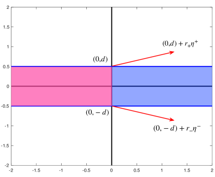
Figure 4: Polar coordinates, $r_{\pm}\eta^{\pm},$ adapted to the locations of the channels.

We now use polar coordinates $r_{\pm}=\sqrt{x_{1}^{2}+(x_{2}\mp d)^{2}}$, adapted to the channel, which is assumed to lie in the set $\{(x_{1},x_{2}):\>-d\leq x_{2}\leq d\},$ see Figure 4. In terms of these coordinates there are outgoing estimates

$$(\partial_{r_{\pm}}-ik)u_{cj}^{l,r}(r_{\pm}\eta^{\pm}\pm(0,d))=O(r_{\pm}^{-\frac{3}{2}})$$ (105)

for $0<\pm\eta^{\pm}_{2}<1$; these are uniform when $\pm\eta^{\pm}_{1}\to 1^{-}$ and $\pm\eta^{\pm}_{1}\to 0^{+}$. Moreover, when $x_{2}$ is bounded,

$$(\pm\partial_{x_{1}}-ik)u_{cj}^{l,r}(x_{1},x_{2})=O(x_{1}^{-\frac{3}{2}}).$$ (106)

Choose a monotone function $\psi_{+}\in\mathcal{C}^{\infty}(\mathbb{R})$ with $\psi_{+}=0$ for $x_{2}<d+1$ and $1$ for $x_{2}>d+2$, and set

$$\psi_{0}(x_{2})=1-(\psi_{+}(x_{2})+\psi_{+}(-x_{2})).$$ (107)

The operators

$$D_{\pm}=\psi_{+}(x_{2})\partial_{r_{+}}\pm\psi_{0}(x_{2})\partial_{x_{1}}+\psi_{+}(-x_{2})\partial_{r_{-}}\in\Psi_{3\operatorname{sc}}^{1,0}(\overline{\mathbb{R}^{2}_{\pm}}_{\operatorname{WG}}),$$ (108)

and have normal symbols $i\tau.$ From the estimates above it follows that

$$(D_{\pm}-ik)u^{l,r}_{cj}(r\eta)=O(r^{-\frac{3}{2}})\text{ for }j=0,1.$$ (109)

Using Vasy’s description of the wave-front set, this implies

$$WF_{3\operatorname{sc}}(u_{cj}^{l,r})\upharpoonright_{\boldsymbol{R}^{2}_{\pm}}\subset R^{+}_{k^{2},\operatorname{mf}}\cup\{\tau=k\}_{\operatorname{ff}}\cap\{\pm x_{1}>0\},$$ (110)

as required. To verify the outgoing conditions for these terms in the sense of Isozaki, we refer to Appendix A. There we compute the conic Fourier transform of the leading term in the asymptotic expansion of a classically outgoing solution and show that it satisfies Isozaki’s outgoing condition. The higher order terms of the expansion belong to $L^{2}(\mathbb{R}^{2})$ and hence also satisfy Isozaki’s condition.

It remains then to discuss the wave-front set over the points where $\eta_{1}=0.$ As a brief preview of the argument, the key point, proved in [21], is that the scattering wave-front sets of formal solutions have a certain regularity which is obtained from a propagation of singularities theorem. This regularity shows that there cannot be any ‘isolated’ parts of this wave-front set over $\eta_{1}=0$. This is further explained in the proof of Theorem 3.

The foregoing analysis leads to the expected uniqueness result for the integral equations introduced in [7] for the solution of the transmission problem in (88). As noted above, the solutions to the transmission problem are expressed as

$$u^{l,r}=-\mathcal{E}^{l,r\,^{\prime}}\sigma+\mathcal{E}^{l,r}\tau,$$ (111)

where

$$\mathcal{E}^{l,r}\tau=\mathcal{S}_{k}\tau+\mathcal{W}^{l,r}\tau,\text{ and }\mathcal{E}^{l,r\,^{\prime}}\sigma=\mathcal{D}_{k}\sigma+\mathcal{W}^{l,r\,^{\prime}}\sigma.$$ (112)

The integral equations along $\{x_{1}=0\}$ then take the form

$$\left(\begin{matrix}\operatorname{Id}&D\\ C&\operatorname{Id}\end{matrix}\right)\left(\begin{matrix}\sigma\\ \tau\end{matrix}\right)=\left(\begin{matrix}g\\ h\end{matrix}\right).$$ (113)

We refer to Section 5 of [7] for further details. Using the uniqueness of the outgoing solution we can finally complete the analysis of this system of equations.

Theorem 3.

For any $0<\alpha<\frac{1}{2},$ and $(g,h)\in\mathcal{C}_{\alpha}(\mathbb{R})\oplus\mathcal{C}_{\alpha+\frac{1}{2}}(\mathbb{R})$ the equation in (113) has a unique solution $(\sigma,\tau)\in\mathcal{C}_{\alpha}(\mathbb{R})\oplus\mathcal{C}_{\alpha+\frac{1}{2}}(\mathbb{R}).$

Remark 8.

The proof is quite similar to the proof of Theorem 3.41 in [5].

Proof.

In [7] it is shown that the equations in (113) are Fredholm integral equations of second kind on the spaces $\mathcal{C}_{\alpha}(\mathbb{R})\oplus\mathcal{C}_{\alpha+\frac{1}{2}}(\mathbb{R}),$ for any $0<\alpha<\frac{1}{2}.$ It therefore suffices to show that the null-space is trivial. Let $(\sigma,\tau)$ satisfy (113) with $(g,h)=(0,0).$ In this circumstance Theorem 1 of [8] shows that $\sigma$ and $\tau$ have asymptotic expansions as $\pm x_{2}\to\infty,$

$$\begin{split}&\sigma(x_{2})=\frac{e^{ik|x_{2}|}}{|x_{2}|^{\frac{1}{2}}}\sum_{l=0}^{N}\frac{a^{\pm}_{l}}{|x_{2}|^{l}}+O\left(|x_{2}|^{-N-\frac{3}{2}}\right),\\ &\tau(x_{2})=\frac{e^{ik|x_{2}|}}{|x_{2}|^{\frac{3}{2}}}\sum_{l=0}^{N}\frac{b^{\pm}_{l}}{|x_{2}|^{l}}+O\left(|x_{2}|^{-N-\frac{5}{2}}\right),\end{split}$$ (114)

for any $N>0.$ The existence of these expansions then implies that the solutions $u^{l,r}$ satisfy the outgoing estimates in Theorems 2 and 3 of [8]. Given the homogeneous transmission condition, the function

$$u^{\operatorname{tot}}(x_{1},x_{2})=\begin{cases}u^{l}(x_{1},x_{2})\text{ for }x_{1}\leq 0,\\ u^{r}(x_{1},x_{2})\text{ for }x_{1}\geq 0\end{cases}$$ (115)

defines a weak solution to $(\Delta+q(x_{1},x_{2})+k^{2})u^{\operatorname{tot}}=0,$ smooth away from $\{x_{1}=0,|x_{2}|<d\}$.

The analysis above shows that $\operatorname{WF}_{3\operatorname{sc}}(u^{\operatorname{tot}})\upharpoonright_{\{\eta_{1}\neq 0\}}\subset R^{+}_{k^{2},\operatorname{mf}}\cup\{\tau=k\}_{\operatorname{ff}}.$ Melrose’s propagation results exclude the possibility of a non-trivial intersection with $\Sigma_{k^{2},\operatorname{mf}}\setminus R^{-}_{k^{2},\operatorname{mf}}\cup R^{+}_{k^{2},\operatorname{mf}},$ but, a priori, it is possible that $\operatorname{WF}_{3\operatorname{sc}}(u^{\operatorname{tot}})$ over $\eta_{1}=0$ intersects $R^{-}_{k^{2},\operatorname{mf}}$ non-trivially. Note that $q(x)=0$ in conic neighborhoods of $\{\eta_{2}=\pm 1\}$ and therefore Proposition 2.8 of [20] shows that $u^{\operatorname{tot}}$ has asymptotic expansions, in neighborhoods of $\eta_{2}=\pm 1,$ of the form

$$u^{\operatorname{tot}}(r\eta)\sim\frac{e^{ikr}}{r^{\frac{1}{2}}}\sum_{j=0}^{\infty}\frac{a_{j}^{+}(\eta)}{r^{j}}+\frac{e^{-ikr}}{r^{\frac{1}{2}}}\sum_{j=0}^{\infty}\frac{a_{j}^{-}(\eta)}{r^{j}},$$ (116)

with $a^{\pm}_{j}(\eta)$ smooth functions of $\eta.$ Since all terms $a^{-}_{j}(\eta)=0,$ for $\eta_{2}\neq\pm 1,$ the $e^{-ikr}$-term is absent, and $u^{\operatorname{tot}}$ is everywhere outgoing and therefore $u^{\operatorname{tot}}\equiv 0.$

To show that the data must be zero we interchange the roles of left and right defining

$$\begin{split}v^{r}(x_{1},x_{2})&=-\mathcal{E}^{l\,^{\prime}}\sigma(x_{1},x_{2})+\mathcal{E}^{l}\tau(x_{1},x_{2})\text{ for }x_{1}\geq 0,\\ v^{l}(x_{1},x_{2})&=\mathcal{E}^{r\,^{\prime}}\sigma(x_{1},x_{2})-\mathcal{E}^{r}\tau(x_{1},x_{2})\text{ for }x_{1}\leq 0.\end{split}$$ (117)

Note the sign change in the definition of $v^{l}.$ As the functions

$$\mathcal{W}^{l,r}f(x_{1},x_{2}),\mathcal{W}^{l,r\,^{\prime}}f(x_{1},x_{2}),\partial_{x_{1}}\mathcal{W}^{l,r\,^{\prime}}f(x_{1},x_{2})$$

are continuous across $x_{1}=0,$ it is elementary to show, using the classical jump relations for $\mathcal{S}_{k}$ and $\mathcal{D}_{k},$ that

$$v^{r}(0,x_{2})=v^{l}(0,x_{2})=-\sigma(x_{2})\text{ and }\partial_{x_{1}}v^{r}(0,x_{2})=\partial_{x_{1}}v^{l}(0,x_{2})=\tau(x_{2}).$$ (118)

The analysis used to show that $u^{\operatorname{tot}}$ is outgoing applies equally well to

$$v^{\operatorname{tot}}(x_{1},x_{2})=\begin{cases}v^{l}(x_{1},x_{2})\text{ for }x_{1}\leq 0,\\ v^{r}(x_{1},x_{2})\text{ for }x_{1}\geq 0,\end{cases}$$ (119)

which also satisfies homogeneous jump conditions. This function is therefore an outgoing solution to

$$(\Delta+q(-x_{1},x_{2})+k^{2})v^{\operatorname{tot}}=0,$$ (120)

which must also vanish. From (118) it follows that $\sigma=\tau=0.$ ∎

We can use a similar argument to show that the solution $u^{\operatorname{tot}}$ defined in (90), for certain of incoming data, agrees with the limiting absorption solution. The simplest case is when $u^{\operatorname{in}}_{r}=0$ and

$$u^{\operatorname{in}}_{l}(x_{1},x_{2})=\sum_{j=0}^{N_{l}}c_{l}v_{l}(x_{2})e^{ix_{1}\sqrt{k^{2}+E_{l,j}^{2}}},$$ (121)

is a sum of incoming wave-guide modes from the left. In this case the integral equations in (113) are solvable and the solutions $(\sigma,\tau)$ have asymptotic expansions like those in (114). The functions $u^{l,r}$ defined in (89), which are solutions to $(\Delta+q_{l,r}+k^{2})u^{l,r},$ are outgoing in their respective half spaces.

To use the limiting absorption principle, we choose a function $\varphi\in\mathcal{C}^{\infty}(\mathbb{R}^{2}),$ supported in $x_{1}<0,$ which equals 1 in a conic neighborhood $(-\infty,-1)\times\{0\}.$ With $w=(\Delta+k^{2}+q_{l})[\varphi u^{\operatorname{in}}_{l}]\in\mathcal{S}(\mathbb{R}^{2}),$ we let

$$u^{\operatorname{out}}=-(\Delta+k^{2}+q+i0^{+})^{-1}w$$ (122)

be the unique outgoing solution, and set $u_{\operatorname{LAP}}=u^{\operatorname{out}}+\varphi u^{\operatorname{in}}_{l}.$ It is clear that

$$(\Delta+k^{2}+q)(u_{\operatorname{LAP}}-u^{\operatorname{tot}})=0,$$ (123)

and $u_{\operatorname{LAP}}-u^{\operatorname{tot}}$ is outgoing everywhere, except possibly over $\{\eta_{2}=\pm 1\}.$ The argument used in the proof of Theorem 3 applies to show that, in fact, this difference is everywhere outgoing, and therefore $u_{\operatorname{LAP}}\equiv u^{\operatorname{tot}}.$

A similar argument applies with data defined by an incoming wave packet, as described in Section 6 of Part I. As the description of this data would require a lengthy discussion, we leave this case to the interested reader. Generally speaking, the solutions found using the integral equations in (90) are outgoing provided the data $(g,h)$ is itself outgoing. This means that it has a finite order asymptotic expansion, like (60) or (61) in [8], which implies that the sources $(\sigma,\tau)$ also have such expansions. While we have not given the details, finite order expansions suffice because we only need to know that (80) or, equivalently, (31) holds for an $l>-\frac{1}{2}.$

6 Conclusion

This paper concludes our introduction of mathematical foundations for the problem of scattering scalar waves from open wave-guides. We have shown that this problem has physically motived, practically verifiable radiation conditions, which imply uniqueness, and that the limiting absorption principle holds as well. In [7, 8] we have presented an effective method to solve a particular model wave-guide problem, which is in the process of being implemented numerically.

There are obviously many directions for further developments in this field. An important applied problem is the development of more flexible numerical methods that apply to more complex geometries in 2 and 3 dimensions. Once numerically implemented, the method presented in [7, 8] can serve as a ‘gold standard’ for new methods that may be more difficult to rigorously analyze. We also hope to establish the existence of complete asymptotic expansions for outgoing solutions, which are valid in neighborhoods of the channel ends.

Another important direction is the study of the full scattering operator defined by the wave guide problem. While its general properties can be obtained using the geometric microlocal methods of Melrose and Vasy, it will be necessary in applications to develop more explicit methods to estimate the relative sizes of the different components of the scattering operator, i.e., to measure how much radiation escapes in the channels vs. in the free regions. This could be quite useful for the practical design of ‘optimal’ wave-guide networks. In Appendix B we show that the channel-to-channel scattering coefficients are well defined.

The methods introduced here readily generalize to study the open wave guide problem for Maxwell’s equations. On the free boundary, the scattering wave-front set readily generalizes to this setting, as does the notion of polarization of the principal singularities, see [6]. The classical Silver-Müller radiation conditions are easily understood in this language. It seems quite likely that channels can again be accommodated, though the details have not yet been worked out.

Appendix A Appendix: Conic Fourier Transform of a Classically Outgoing Solution

In this appendix we carry out a relatively elementary but lengthy computation showing that the leading term in the asymptotic expansion of a classically outgoing solution in two dimensions satisfies Isozaki’s radiation condition. In [11, Lemma 1.4] Isozaki proves this abstractly. The corresponding fact is also straightforward in Vasy’s formulation using the observation that $\operatorname{WF}_{3\operatorname{sc}}(v)\subset\Sigma_{k^{2}}\cap\{\tau=k\}=R^{+}_{k^{2}}.$

This leading term takes the form $v(r,\theta)=a(\theta)e^{ikr}/\sqrt{r},$ where $a\in\mathcal{C}^{\infty}(\partial\overline{\mathbb{R}^{2}})$. We compute its conic Fourier transform around any ray $r\zeta(\theta_{0})$, $r>0$, where we let

$$\zeta(\theta)=(\cos\theta,\sin\theta).$$

For simplicity of notation we may as well assume that $\theta_{0}=0$, which we do below.

Multiply $v$ by smooth localizing functions $\psi_{+}(r)$ and $\varphi(\theta)$; here $\psi_{+}(r)$ vanishes for $r<1$ and equals $1$ for $r>2$, and $\varphi$ is supported in $(-\delta,\delta)$ with $\varphi(\theta)=1$ when $|\theta|<\delta/2.$ The integral defining the conic Fourier transform converges if we replace $k$ by $k+i\sigma$, $\sigma>0$, to get

$$\hat{v}_{\sigma}(\xi)=\int\frac{a(\theta)\psi_{+}(r)\varphi(\theta)e^{i(kr-y\cdot\xi)}e^{-r\sigma}}{\sqrt{r}}\,rdrd\theta.$$ (124)

Our goal is to compute the distributional limit $\hat{v}=\lim_{\sigma\to 0^{+}}\hat{v}_{\sigma}.$ We show below that $\hat{v}$ is rapidly decreasing along with all its derivatives as $|\xi|\to\infty$, and that it is smooth outside any fixed ball $B_{\nu}(k,0)$, $\nu>0$, provided $\delta$ is chosen sufficiently small. Denoting by $\chi_{-}$ the same function as in (98), these facts show that, with $\epsilon$ and $\delta$ chosen small enough,

$$Av(x)=\int\chi_{-}\left(\frac{x}{|x|}\cdot\xi\right)\hat{v}(\xi)e^{ix\cdot\xi}\,d\xi$$ (125)

decreases rapidly for $x$ in a cone $C_{\delta^{\prime}}=\{r\zeta(\theta):\>|\theta|<\delta^{\prime},\ r>0\}$. This is Isozaki’s outgoing radiation condition.

To prove this we set $x=r\zeta(\theta)$ and $\xi=\rho\zeta(\phi)$, so that

$$\hat{v}_{\sigma}(\xi)=\int_{-\delta}^{\delta}\int_{1}^{\infty}a(\theta)\psi_{+}(r)\varphi(\theta)e^{ir(k-\rho\cos(\theta-\phi))}e^{-r\sigma}\sqrt{r}\,drd\theta.$$ (126)

Using $\partial_{\theta}e^{-ir\rho\cos(\theta-\phi)}=ir\rho\sin(\theta-\phi)e^{-ir\rho\cos(\theta-\phi)}$, we can integrate by parts in $\theta$ as often as we like to obtain

$$\begin{split}\hat{v}_{\sigma}(\rho,\phi)=\int_{1}^{\infty}\int_{-\delta}^{\delta}&\left(\partial_{\theta}\frac{-1}{ir\rho\sin(\theta-\phi)}\right)^{N}(a(\theta)\varphi(\theta))\\ &e^{ir(k-\rho\cos(\theta-\phi))}\psi_{+}(r)e^{-r\sigma}\sqrt{r}\,d\theta\,dr.\end{split}$$ (127)

Now let $\sigma\to 0^{+}$ to conclude that $\hat{v}(\rho,\phi)$ is rapidly decreasing and smooth in the double cone

$$V_{\delta}=\{(\rho,\phi):\>|\phi|>2\delta\ \mbox{and}\ |\phi-\pi|>2\delta,\ \rho\neq 0\}.$$

Next, since

$$\partial_{r}e^{ir(k-\rho\cos(\theta-\phi)+i\sigma)}=i(k-\rho\cos(\theta-\phi)+i\sigma)e^{ir(k-\rho\cos(\theta-\phi)+i\sigma)},$$

we can integrate by parts in $r$ as often as we like when $\rho<k$ to get

$$\begin{split}\hat{v}_{\sigma}(\rho,\phi)&=\int_{-\delta}^{\delta}\int_{1}^{\infty}(a(\theta)\varphi(\theta))e^{ir(k-\rho\cos(\theta-\phi))}e^{-r\sigma}\\ &\left[\frac{-1}{i(k-\rho\cos(\theta-\phi)+i\sigma)}\,\partial_{r}\right]^{N}(\psi_{+}(r)\sqrt{r})\,drd\theta.\end{split}$$ (128)

The resulting integrand is bounded independently of $\sigma\geq 0$ by $C_{N}r^{\frac{1}{2}-N}$, thus we can let $\sigma\to 0^{+}$ and again conclude that $\hat{v}(\rho,\phi)\in\mathcal{C}^{\infty}$ when $\rho<k$.

Next, if $|\phi-\pi|<2\delta$, then $\cos(\theta-\phi)<\cos(3\delta-\pi)$, and this is strictly negative when $\delta\ll 1$, so we can again integrate by parts in $r$ to conclude that $\hat{v}(\rho,\phi)$ is smooth and rapidly decreasing in the cone $\{|\phi-\pi|\leq 2\delta\}.$ Finally, when $|\phi|\leq 2\delta,$ then $\rho\cos(\theta-\phi)>\rho\cos(3\delta).$ If $\rho>\frac{k}{\cos(3\delta)},$ then a final integration by parts shows that $v(\rho,\phi)$ is smooth and rapidly decreasing in the set $\{|\phi|\leq 2\delta,\rho>\frac{k}{\cos(3\delta)}\}.$

Combining all these estimates, we conclude that for any $\nu>0,$ there exists a $\delta>0$ so that $\hat{v}\in\mathcal{C}^{\infty}(\mathbb{R}^{2}\setminus B_{\nu}(k,0)),$ and is rapidly decreasing with all derivatives as $\rho\to\infty.$

Now consider $Av(x)$ as in (125), where $x\in C_{\delta^{\prime}}=\{r\zeta(\theta):\>|\theta|<\delta^{\prime},r>0\}$ for some appropriate $\delta^{\prime}>0.$ The integrand is supported in $\{\xi:\omega\cdot\xi<2\epsilon\}.$ Thus by choosing $\nu\ll k,$ and $\epsilon<\nu,$ we can then choose $\delta^{\prime}>0$ so that when $x\in C_{\delta^{\prime}},$ the integrand in $Av(x)$ is a smooth, rapidly decreasing function of $\xi$ with support a fixed positive distance from $B_{\nu}(k,0).$ Thus $Av(x)$ is also rapidly decreasing as $|x|\to\infty$, so $v$ satisfies Isozaki’s outgoing condition.

Referring back to the notation of Section 5, these calculations suffice to handle the terms arising from $u_{0}^{l,r},u_{1}^{l,r}$ and $u_{c0}^{l,r},u_{c1}^{l,r}$ away from the ends of the channels. Similar, though more complicated, calculations handle the contributions involving $u_{c0}^{l,r},u_{c1}^{l,r}$ in neighborhoods of the channels. We leave these estimates to the interested reader.

Appendix B Channel-to-Channel Scattering Coefficients

A fundamental question of scattering theory for open wave-guides is to understand how an incoming wave-guide mode is scattered by the network of wave-guides into a sum of outgoing wave-guide modes and radiation. Here we consider the wave-guide mode portion of the scattered field. To formulate this question mathematically, we now construct the appropriate class of solutions using the various tools we have been discussing. For each $\alpha\in\mathcal{A},$ choose a conic cutoff function $\varphi_{\alpha}$ which equals $1$ in the exterior of a large ball $B_{2R}(0)$ intersected with a conic region around $v_{\alpha}$ and which has support outside $B_{R}(0)$ and conic neighborhoods of all the other $v_{\beta}$. Thus $q(x)=q_{\alpha}(x^{\alpha})$ in $\operatorname{supp}\varphi_{\alpha}.$

Now consider an incoming wave-guide mode associated to this channel and localized to this neighborhood; applying the operator to it yields a rapidly vanishing function

$$f_{\alpha,j}=(\Delta+q+k^{2})\left[\varphi_{\alpha}(x)e^{-ix_{\alpha}\sqrt{E^{2}_{\alpha,j}+k^{2}}}u_{\alpha,j}(x^{\alpha})\right]\in\mathcal{S}(\mathbb{R}^{d}).$$ (129)

We now apply the outgoing resolvent to obtain the outgoing solution, $v^{+}_{\alpha,j},$ to

$$(\Delta+q+k^{2})v^{+}_{\alpha,j}=f_{\alpha,j}.$$ (130)

The difference $w_{\alpha,j}=e^{-ix_{\alpha}\sqrt{E^{2}_{\alpha,j}+k^{2}}}u_{\alpha,j}(x^{\alpha})-v^{+}_{\alpha,j}$ is then a generalized eigenfunction:

$$(\Delta+q+k^{2})w_{\alpha,j}=0.$$ (131)

It has an incoming component along the $v_{\alpha}$ channel and a superposition of outgoing components in all of the channels, along with outgoing radiation.

We seek a formula for the outgoing guided-mode contributions. We can isolate the component corresponding to any wave-guide mode $u_{\beta,l}(x^{\beta})$ with energy $E^{2}_{\beta,l}$ by taking the inner product localized along that channel. This gives a function

$$s_{\alpha,j;\beta,l}(x_{\beta})=\int_{\mathbb{R}^{d-1}}\varphi_{\beta}(x_{\beta},x^{\beta})v^{+}_{\alpha,j}(x_{\beta},x^{\beta})\overline{u_{\beta,l}(x^{\beta})}dx^{\beta}$$ (132)

which vanishes by construction when $x_{\beta}<R.$ Below we show below that it satisfies

$$s_{\alpha,j;\beta,l}(x_{\beta})=S_{\alpha,j;\beta,l}e^{ix_{\beta}\sqrt{E_{\beta,l}^{2}+k^{2}}}+\sigma(x_{\beta}),\qquad\sigma\in\mathcal{S}(\mathbb{R}).$$ (133)

We can thus define the scattering coefficient $S_{\alpha,j;\beta,l}$ between the incoming mode $(\alpha,j)$ and outgoing mode $(\beta,l)$ by

$$S_{\alpha,j;\beta,l}=\lim_{x_{\beta}\to\infty}e^{-ix_{\beta}\sqrt{E_{\beta,l}^{2}+k^{2}}}s_{\alpha,j;\beta,l}(x_{\beta}).$$ (134)

We must verify (133) and show that this limit is independent of all choices made in its definition.

The independence of choice of cut-offs is easily established. If $\{\varphi_{\alpha}^{\prime}:\>\alpha\in\mathcal{A}\}$ is another collection of conic cutoff functions, with corresponding outgoing solutions $v_{\alpha,j}^{+^{\prime}}$ and projections $\{s_{\alpha,j;\beta,l}^{\prime}(x_{\beta})\}$ as in (133), then the difference $(v_{\alpha,j}^{+}-v_{\alpha,j}^{+^{\prime}})$ is the unique outgoing solution to

$$(\Delta+q+k^{2})v=(\Delta+q+k^{2})\left[(\varphi_{\alpha}-\varphi_{\alpha}^{\prime})e^{-ix_{\alpha}\sqrt{E^{2}_{\alpha,j}+k^{2}}}u_{\alpha,j}(x^{\alpha})\right].$$ (135)

The difference on the right is rapidly decreasing, hence a fortiori outgoing. Thus by uniqueness of outgoing solutions, we see that

$$(v_{\alpha,j}^{+}-v_{\alpha,j}^{+^{\prime}})=\left[(\varphi_{\alpha}-\varphi_{\alpha}^{\prime})e^{-ix_{\alpha}\sqrt{E^{2}_{\alpha,j}+k^{2}}}u_{\alpha,j}(x^{\alpha})\right],$$ (136)

hence

$$s_{\alpha,j;\beta,l}(x_{\beta})-s_{\alpha,j;\beta,l}^{\prime}(x_{\beta})\in\mathcal{S}(\mathbb{R}),$$ (137)

so the coefficients $\{S_{\alpha,j;\beta,l}\}$ are well defined.

We next establish (133). Using $(\Delta_{\beta}+q_{\beta}(x^{\beta}))u_{\beta,l}=E_{\beta,l}^{2}u_{\beta,l}$, we write

$$\begin{split}s_{\alpha,j;\beta,l}(x_{\beta})=&\\ \frac{1}{E_{\beta,l}^{2}}&\int\varphi_{\beta}(x_{\beta},x^{\beta})v^{+}_{\alpha,j}(x_{\beta},x^{\beta})\overline{(\Delta_{\beta}+q_{\beta}(x^{\beta}))u_{\beta,l}(x^{\beta})}dx^{\beta}.\end{split}$$ (138)

The function $\varphi_{\beta}(x_{\beta},x^{\beta})v_{\alpha,j}(x_{\beta},x^{\beta})$ is smooth with bounded derivatives, and $u_{\beta,l}(x^{\beta})$ decays exponentially, so we can integrate by parts to obtain:

$$s_{\alpha,j;\beta,l}(x_{\beta})=\frac{1}{E_{\beta,l}^{2}}\int(\Delta_{\beta}+q_{\beta}(x^{\beta}))\left[\varphi_{\beta}(x_{\beta},x^{\beta})v^{+}_{\alpha,j}(x_{\beta},x^{\beta})\right]\overline{u_{\beta,l}(x^{\beta})}dx^{\beta}.$$ (139)

Using (130), we see that

$$s_{\alpha,j;\beta,l}(x_{\beta})=-\frac{1}{E_{\beta,l}^{2}}(\partial_{x_{\beta}}^{2}+k^{2})\int\varphi_{\beta}v^{+}_{\alpha,j}\overline{u_{\beta,l}(x^{\beta})}dx^{\beta}+\\ \frac{1}{E_{\beta,l}^{2}}\int\Bigg{[}\varphi_{\beta}f_{\alpha,j}+\Delta\varphi_{\beta}v^{+}_{\alpha,j}+2\nabla\varphi_{\beta}\cdot\nabla v^{+}_{\alpha,j}-\varphi_{\beta}(q-q_{\beta})v^{+}_{\alpha,j}\Bigg{]}\overline{u_{\beta,l}(x^{\beta})}dx^{\beta}.$$ (140)

From this and the support properties of the $q_{\alpha}$ and conic cut-offs $\varphi_{\alpha}$, it follows that

$$(\partial_{x_{\beta}}^{2}+k^{2}+E_{\beta,l}^{2})s_{\alpha,j;\beta,l}=g\in\mathcal{S}(\mathbb{R}).$$ (141)

A standard analysis of this one-dimensional problem shows that there are constants $a,b,$ and smooth functions $h_{0},h_{1}$ supported in the positive half-line with $h_{0}(t)=1$ for sufficiently large $t$ and $h_{1}$ Schwartz class, such that

$$s_{\alpha,j;\beta,l}(x_{\beta})=h_{0}(x_{\beta})\left[ae^{ix_{\beta}\sqrt{E_{\beta,l}^{2}+k^{2}}}+be^{-ix_{\beta}\sqrt{E_{\beta,l}^{2}+k^{2}}}\right]+h_{1}(x_{\beta}).$$ (142)

To establish (133), it remains to show that $b=0.$ For any integrable function $m(x^{\beta})$, denote by $\widetilde{m}(\xi^{\beta})$ its $(d-1)$-dimensional Fourier transform. Since $u_{\beta,l}\in\mathcal{S}(\mathbb{R}^{d-1})$ we can apply the Plancherel formula to rewrite

$$s_{\alpha,j;\beta,l}(x_{\beta})=\frac{1}{(2\pi)^{d-1}}\int_{\mathbb{R}^{d-1}}\widetilde{\varphi_{\beta}v^{+}_{\alpha,j}}(x_{\beta},\xi^{\beta})\overline{\widetilde{u}_{\beta,l}(\xi^{\beta})}d\xi^{\beta}.$$ (143)

Taking the Fourier tranform in $x_{\beta}$ now gives

$$\begin{split}\frac{1}{(2\pi)^{d-1}}\int_{\mathbb{R}^{d-1}}&\widehat{\varphi_{\beta}v^{+}_{\alpha,j}}(\xi_{\beta},\xi^{\beta})\overline{\widetilde{u}_{\beta,l}(\xi^{\beta})}d\xi^{\beta}=\\ &a\mathcal{F}(h_{0}e^{ix_{\beta}\sqrt{E_{\beta,l}^{2}+k^{2}}})+b\mathcal{F}(h_{0}e^{-ix_{\beta}\sqrt{E_{\beta,l}^{2}+k^{2}}})+\hat{h}_{1}(\xi_{\beta}).\end{split}$$ (144)

It follows that there are non-zero constants $c_{0},c_{1}$ and a function $h_{2}\in\mathcal{S}(\mathbb{R})$ so that

$$\mathcal{F}(h_{0}e^{-ix_{\beta}\sqrt{E_{\beta,l}^{2}+k^{2}}})=\\ c_{0}\delta\left(\xi_{\beta}+\sqrt{E_{\beta,l}^{2}+k^{2}}\right)+c_{1}\operatorname{PV}\frac{\widehat{h_{0}^{\prime}}(\xi_{\beta})}{\xi_{\beta}+\sqrt{E_{\beta,l}^{2}+k^{2}}}+h_{2}(\xi_{\beta}),$$ (145)

Using the outgoing condition we see that if $\varphi_{\beta}$ has sufficiently small conic support, then

$$\frac{1}{(2\pi)^{d-1}}\int_{\mathbb{R}}\int_{\mathbb{R}^{d-1}}\widehat{\varphi_{\beta}v^{+}_{\alpha,j}}(\xi_{\beta},\xi^{\beta})\chi_{-}(\xi_{\beta})\overline{\widetilde{u}_{\beta,l}(\xi^{\beta})}e^{ix_{\beta}\xi_{\beta}}d\xi^{\beta}d\xi_{\beta}$$ (146)

is rapidly decreasing as $x_{\beta}\to\infty.$ This is because $\chi_{-}(\omega\cdot\xi)\overline{\widetilde{u}_{\beta,l}(\xi^{\beta})}$ belongs to Isozaki’s symbol class $\mathcal{R}_{-}(\epsilon),$ and $(x_{\beta},0)\cdot\xi=x_{\beta}\xi_{\beta}.$ By (145), this is only possible if $b=0.$

This completes the proof that the incoming-to-outgoing wave-guide mode scattering coefficients, $\{S_{\alpha,j;\beta,l}:\>\alpha,\beta\in\mathcal{A}\},$ are well-defined. These coefficients depend on the choice of origin for $\mathbb{R}^{d}$ as well as the choice of orthonormal basis for the incoming and outgoing wave-guide modes. Translating the origin by $x_{0},$ has the effect of replacing $S_{\alpha,j;\beta,l}$ by

$$e^{i\left[x_{0}\cdot v_{\alpha}\sqrt{E_{\alpha,j}^{2}+k^{2}}-x_{0}\cdot v_{\beta}\sqrt{E_{\beta,l}^{2}+k^{2}}\right]}S_{\alpha,j;\beta,l},$$ (147)

which is conjugation by a diagonal unitary matrix. It remains a very interesting problem to give effective estimates for these coefficients, and to bound the portion of the energy of the incoming signal that is dissipated in radiation.

The ‘full’ scattering operator involves both radiation and wave-guide modes. In [21] the free-to-free part of the scattering operator is described in considerable detail. In [10] various other parts of the scattering operator are described for the $N$-body Schrödinger case. However, it is an interesting and important challenge to assemble all of this into a more coherent and complete study of the full scattering operator for open wave-guides

References

- [1] A.-S. Bonnet-Bendhia, B. Goursaud, and C. Hazard, Mathematical analysis of the junction of two acoustic open waveguides, SIAM J. Appl. Math., 71 (2011), pp. 2048–2071.
- [2] A.-S. Bonnet-Bendhia and A. Tillequin, A limiting absorption principle for scattering problems with unbounded obstacles, Math. Methods Appl. Sci., 24 (2001), pp. 1089–1111.
- [3] S. Chandler-Wilde, P. Monk, and M. Thomas, The mathematics of scattering by unbounded, rough, inhomogeneous layers, J. Comput. Appl. Math., 204 (2007), pp. 549–559.
- [4] S. Chandler-Wilde and B. Zhang, Electromagnetic scattering by an inhomogeneous conducting or dielectric layer on a perfectly conducting plate, R. Soc. Lond. Proc. Ser. A Math. Phys. Eng. Sci., 454 (1998), pp. 519–542.
- [5] D. Colton and R. Kress, Integral Equation Methods in Scattering Theory, Krieger Publishing Co., Malabar, Florida, reprint ed., 1992.
- [6] N. Dencker, On the Propagation of Polarization Sets for Systems of Real Principal Type, J.F.A., 46 (1982), pp. 351–372.
- [7] C.L. Epstein, Solving the Scattering Problem for Open Wave-guides, I: Fundamental Solutions and Integral Equations, arXiv:2302.04353 [math-ph], 2023.
- [8] C.L. Epstein, Solving the Scattering Problem for Open Wave-guides, II: Outgoing Estimates, arXiv:2310.05816 [math-ph], 2023.
- [9] C. Gérard, H. Isozaki, and E. Skibsteb, Commutator algebra and resolvent estimates, Spectral and Scattering Theory and Related Topics, Adv. Stud. Pure Math. 23, Academic Press, Boston, 1994.
- [10] H. Isozaki, Structure of S-Matrices for Three Body Schrödinger Operators, Comm. Math. Phys., 146 (1992), p. 241-258.
- [11] H. Isozaki, A generalization of the radiation condition of Sommerfeld for -body Schrödinger operators, Duke Math. Jour., 74 (1994), p. 557–584.
- [12] E.M. Kartchevski, A.I. Nosich, and G.W. Hanson, Mathematical analysis of the generalized natural modes of an inhomogeneous optical fiber SIAM Journal on Applied Mathematics, 65(6), (2005) p. 2033-2048.
- [13] R.B. Melrose, Spectral and Scattering Theory for the Laplacian on Asymptotically Euclidean Spaces in Spectral and Scattering Theory, Ed. M. Ikawa, (1994), CRC Press, 46 p. 85-130.
- [14] R.B. Melrose, Geometric Scattering Theory, Cambridge Univ. Press, Cambridge, 1995.
- [15] R.B. Melrose and M. Zworski, Scattering metrics and geodesic flow at infinity, Invent Math. 124 (1996), p. 389-436.
- [16] A.I. Nosich, Radiation conditions, limiting absorption principle, and general relations in open waveguide scattering, Journal of Electromagnetic Waves and Applications, 8, (1994), p. 329–353.
- [17] P. Perry, I.M. Sigal, and B. Simon, Spectral analysis of N-body Schrödinger operators, Ann. of Math. (2) 114 (1981), p. 519-567.
- [18] F. Rellich, Über das asymptotische Verhalten der Lösungen von in unendlichen Gebieten, Jahr. d. D.M.V., 53(1943), p. 57-64.
- [19] M.E. Taylor, Partial Differential Equations, II, Springer-Verlag, New York, 1996.
- [20] A. Vasy, Asymptotic Behavior of Generalized Eigenfunctions in -Body Scattering, J.F.A. 148 (1997), p. 170-184.
- [21] A. Vasy, Propagation of singularities in three-body scattering, Astèrisque, 262(2000), 158 pp.