Experimental bounds on linear-friction dissipative collapse models from levitated optomechanics

Abstract

Collapse models constitute an alternative to quantum mechanics that solve the well-know quantum measurement problem. In this framework, a novel approach to include dissipation in collapse models has been recently proposed, and awaits experimental validation. Our work establishes experimental bounds on the so-constructed linear-friction dissipative Diósi-Penrose (dDP) and Continuous Spontaneous localisation (dCSL) models by exploiting experiments in the field of levitated optomechanics. Our results in the dDP case exclude collapse temperatures below $10^{-13}$ K and $6\times 10^{-12}$ K respectively for values of the localisation length smaller than $10^{-6}$ m and $10^{-8}$ m. In the dCSL case the entire parameter space is excluded for values of the temperature lower than $6\times 10^{-9}$ K.

I Introduction

Models of spontaneous wavefunction collapse, or simply collapse models Bassi and Ghirardi (2003); Bassi et al. (2013); Carlesso et al. (2022), represent a well established paradigm in the realm of quantum foundations, and constitute a strong figure of merit for the study of the macroscopic limits of quantum mechanics. The key idea of collapse models is that quantum mechanics must be modified to explain the quantum-to-classical transition at macroscopic scales. Thus, they add suitably constructed phenomenological terms to the standard Schrödinger equation. Their action can be seen as that of a noise field that leads to the collapse of the wavefunction. Depending on the specific collapse model, the origin of such a field can be either of unknown origin or be related to the gravitational field.

The two most studied collapse models are the Diósi-Penrose (DP) model Diosi (1987); Penrose (1996) and the Continuous Spontaneous Localisation (CSL) model Pearle (1989); Ghirardi et al. (1990). The latter is parametrised by a collapse rate $\lambda$ and a localisation length $r_{\text{\tiny C}}$. Conversely, the former model, which is related to gravity, is characterised only by a localisation length $R_{0}$ as the collapse rate is fixed by the gravitation constant $G$. Since the predictions of these models deviate from those of standard quantum mechanics, such models can be tested, and experimental bounds can be derived on the values of their free parameters Bilardello et al. (2016); Vinante et al. (2016); Carlesso et al. (2016); Adler et al. (2019); Vinante et al. (2017); Helou et al. (2017); Vinante et al. (2020a); Zheng et al. (2020); Pontin et al. (2020); Donadi et al. (2021a, b); Arnquist et al. (2022). An acknowledged challenge within collapse models is the energy divergence due to the collapse mechanism. To address this concern, dissipative extensions of collapse models were proposed as a solution Smirne and Bassi (2015); Bahrami et al. (2014), implying the existence of a fundamental and universal damping mechanism which can be probed by mechanical systems with very low dissipation Nobakht et al. (2018); Pontin et al. (2020); Vinante et al. (2019).

Recently, a new approach to the introduction of dissipation in collapse model has been proposed Di Bartolomeo et al. (2023). The latter is based on a different mechanism with respect to that previously proposed, namely the linear-friction of the current of the many-body system. Such an approach has not been tested yet. The present work falls within this context.

We derive the first experimental bounds on linear-friction dissipative DP (dDP) and CSL (dCSL) models from levitated optomechanics characterised by ultralow damping Pontin et al. (2020); Vinante et al. (2019); Dania et al. (2023). In particular, for the dDP model, values of the temperature $T_{\beta}$ of the collapse field lower than $10^{-13}$ K and $6\times 10^{-12}$ K are excluded respectively for values of the localisation length smaller than $10^{-6}$ m and $10^{-8}$ m. On the other hand, for the dCSL model, the entire parameter space is excluded for $T_{\beta}$ lower than $6\times 10^{-9}$ K. Finally, we compare the approach recently proposed in Di Bartolomeo et al. (2023) with those previously suggested in Smirne and Bassi (2015); Bahrami et al. (2014), and conclude that they can be in principle experimentally distinguished.

II The model

Here, we briefly present the universal dissipative mechanism for collapse models of many-body systems, which was introduced in Ref. Di Bartolomeo et al. (2023). We start from the following master equation

$$\frac{\operatorname{d}\!}{\operatorname{d}\!t}\hat{\rho}_{t}=-\frac{i}{\hbar}[\hat{H},\hat{\rho}_{t}]+\mathcal{D}\hat{\rho}_{t},$$ (1)

where $\hat{H}$ is the Hamiltonian of the system and

$$\mathcal{D}\hat{\rho}_{t} =\frac{1}{\hbar^{2}}\int\operatorname{d}\!^{3}x\int\operatorname{d}\!^{3}y\,D(\textbf{x}-\textbf{y})\left(\hat{L}(\textbf{x})\hat{\rho}_{t}\hat{L}^{\dagger}(\textbf{y})-\frac{1}{2}\{\hat{L}^{\dagger}(\textbf{x})\hat{L}(\textbf{y}),\hat{\rho}_{t}\}\right).$$ (2)

The dissipation is introduced in the model by considering the following Lindblad operator $\hat{L}(\textbf{x})$

$$\hat{L}(\textbf{x})=\mathrm{\hat{\mu}}(\textbf{x})-i\frac{\hbar\beta}{4}\nabla_{\textbf{x}}{\mathrm{\hat{\textbf{J}}}}(\textbf{x}),$$ (3)

where $\beta$ is a free parameter driving the dissipation mechanism. A similar method has been considered for a gravity-related model in Di Bartolomeo et al. (2021). When $\beta$ is set to zero, one obtains the standard (non-dissipative) collapse master equation. The mass density $\mathrm{\hat{\mu}}(\textbf{x})$ and the current ${\mathrm{\hat{\textbf{J}}}}(\textbf{x})$ in the second-quantization framework respectively read as

$$\mathrm{\hat{\mu}}(\textbf{x})=m\hat{\psi}^{\dagger}(\textbf{x})\hat{\psi}(\textbf{x}),$$ (4a)

$${\mathrm{\hat{\textbf{J}}}}(\textbf{x})=-i\frac{\hbar}{2}\left(\hat{\psi}^{\dagger}(\textbf{x})\nabla_{\textbf{x}}\hat{\psi}(\textbf{x})-\nabla_{\textbf{x}}\hat{\psi}^{\dagger}(\textbf{x})\hat{\psi}(\textbf{x})\right),$$ (4b)

with $\hat{\psi}(\textbf{x})$ being the (fermionic) annihilation field operator. In the following sections we will work in the first-quantization. Thus, for a system of $N$ point-like particles of mass $m$, the mass density and the current can be expressed as

$$\mathrm{\hat{\mu}}(\textbf{x})=m\sum_{j=1}^{N}\delta(\textbf{x}-\hat{\textbf{x}}_{j}),\quad{\mathrm{\hat{\textbf{J}}}}(\textbf{x})=\frac{1}{2}\sum_{j=1}^{N}\Bigl{\{}\hat{\textbf{p}}_{j},\delta(\textbf{x}-\hat{\textbf{x}}_{j})\Bigr{\}},$$ (5)

where $\hat{\textbf{x}}_{j}$ and $\hat{\textbf{p}}_{j}$ are respectively the position and momentum operator of the j-th particle.

The form of the kernel $D(\textbf{x}-\textbf{y})=(2\pi)^{-3}\int{\operatorname{d}\!^{3}k}\,D_{\textbf{k}}e^{i\textbf{k}(\textbf{x}-\textbf{y})}$ in Eq. (2) depends on the specific collapse model. Here we consider the dissipative Diósi-Penrose (dDP) Diosi (1987); Penrose (1996) and the dissipative Continuous Spontaneous localisation (dCSL) Pearle (1989); Ghirardi et al. (1990) models, which correspond respectively to

$$D_{\textbf{k}}=\exp(-\sigma^{2}k^{2})\times\begin{cases}\hbar^{2}\gamma&(\text{CSL}),\\ 4\pi\hbar G/k^{2}&(\text{DP}),\end{cases}$$ (6)

where $k=|\textbf{k}|$. Here, the $k^{-2}$ term in the second expression comes from the Fourier transform of the Newtonian potential $V(\textbf{x}-\textbf{y})=-G/|\textbf{x}-\textbf{y}|$. In the DP model the decoherence rate is set by the Newton constant $G$ and $\sigma=R_{0}$ is a free parameter representing the spatial cut-off due to the regularization procedure. The CSL model can be described in terms of two free parameters being $\gamma=(\sqrt{4\pi}\sigma)^{3}\lambda/m_{0}^{2}$ and $\sigma=r_{\text{\tiny C}}$, which are respectively the collapse rate and localisation length of the model ($m_{0}$ is a reference mass chosen as that of a nucleon).

III Dissipative dynamics of the center of mass of a $N$-particle system

We compute the dynamics of the center of mass of a rigid system made of $N$ particles. For convenience, we rewrite Eq. (2) in the Fourier representation

$$\mathcal{D}\hat{\rho}_{t}=\frac{1}{\hbar^{2}}\int\frac{\operatorname{d}\!^{3}k}{(2\pi)^{3}}D_{\textbf{k}}\left(\hat{L}_{\textbf{k}}\hat{\rho}_{t}\hat{L}_{\textbf{k}}^{\dagger}-\frac{1}{2}\{\hat{L}_{\textbf{k}}^{\dagger}\hat{L}_{\textbf{k}},\hat{\rho}_{t}\}\right),$$ (7)

where now the Lindblad operators become

$$\hat{L}_{\textbf{k}}=\mathrm{\hat{\mu}}_{\textbf{k}}+\frac{\hbar\beta}{4}\textbf{k}{\mathrm{\hat{\textbf{J}}}}_{\textbf{k}},$$ (8)

and the Fourier representation of the mass density and of the current is

$$\mathrm{\hat{\mu}}_{\textbf{k}}=m\sum_{j=1}^{N}e^{i\textbf{k}\hat{\textbf{x}}_{j}},\quad{\mathrm{\hat{\textbf{J}}}}_{\textbf{k}}=\frac{1}{2}\sum_{j=1}^{N}\left\{\hat{\textbf{p}}_{k},e^{i\textbf{k}\hat{\textbf{x}}_{j}}\right\}.$$ (9)

In general the position and momentum operators in Eq. (9) can be written as

$$\hat{\textbf{x}}_{j}=\hat{\textbf{x}}+\textbf{x}_{j}^{(0)}+\Delta\hat{\textbf{x}}_{j},\quad\hat{\textbf{p}}_{j}=\frac{m}{M}\hat{\textbf{p}}+\textbf{p}_{j}^{(0)}+\Delta\hat{\textbf{p}}_{j},$$ (10)

where $\hat{\textbf{x}}$ and $\hat{\textbf{p}}$ are the position and momentum operators of the center of mass, $\textbf{x}_{j}^{(0)}$ and $\textbf{p}_{j}^{(0)}$ are the classical equilibrium position and momentum of the $j$-th particle with respect to the center of mass, and $\Delta\hat{\textbf{x}}_{j}$ and $\Delta\hat{\textbf{p}}_{j}$ are the relative fluctuations, and $M$ is the total mass of the system. Under the assumption of a rigid body, the relative fluctuations are negligible, namely $\Delta\hat{\textbf{x}}_{j}=\Delta\hat{\textbf{p}}_{j}=0$. By substituting Eq. (10) into Eq. (9) and by assuming that the spread of the wavefunction of the center of mass is much smaller than $\sigma$, we can Taylor expand the mass density and the current for small fluctuations of $\hat{\textbf{x}}$, finding

$$\hat{\mu}_{\textbf{k}}\simeq\mu_{\textbf{k}}+i\textbf{k}\mu_{\textbf{k}}\hat{\textbf{x}},$$ (11a)

$${\mathrm{\hat{\textbf{J}}}}_{\textbf{k}}\simeq\textbf{J}_{\textbf{k}}+\frac{\mu_{\textbf{k}}}{M}\hat{\textbf{p}}+i\textbf{k}\textbf{J}_{\textbf{k}}\hat{\textbf{x}}+\frac{i\textbf{k}}{2M}\mu_{\textbf{k}}\{\hat{\textbf{p}},\hat{\textbf{x}}\},$$ (11b)

where $\mu_{\textbf{k}}=m\sum_{j=0}^{N}e^{i\textbf{k}\textbf{x}^{(0)}_{j}}$ and $\textbf{J}_{\textbf{k}}=\sum_{j=0}^{N}\textbf{p}_{j}^{(0)}e^{i\textbf{k}\textbf{x}_{j}^{(0)}}$ are respectively the classical mass density and current of the system in the Fourier representation. We notice that for a rigid body $\textbf{p}_{j}^{(0)}=0$ thus $\textbf{J}_{\textbf{k}}=0$.

For the sake of simplicity, we reduce the problem in one dimension, namely $\hat{\textbf{x}}=(\hat{x},0,0)$ and $\hat{\textbf{p}}=(\hat{p},0,0)$. Moreover, by assuming small k (i.e., $|\textbf{k}|\ll 1/\sigma$) we neglect all the terms of order higher than $O(\textbf{k}^{2})$ and substitute the latter expressions for the mass density and the current in Eq. (7). In such a way, we obtain the following master equation for the motion of the center of mass in the linear limit

$$\frac{\operatorname{d}\!}{\operatorname{d}\!t}\hat{\rho}_{cm}=-\frac{i}{\hbar}[\hat{H},\hat{\rho}_{cm}]+\eta\left(\hat{L}\hat{\rho}_{cm}\hat{L}^{\dagger}-\frac{1}{2}\{\hat{L}^{\dagger}\hat{L},\hat{\rho}_{cm}\}\right),$$ (12)

where $\hat{L}=\hat{x}+i\alpha\hat{p}$ with $\alpha={\Gamma}/{2\eta\hbar}$ and where

$$\Gamma=\frac{\hbar^{2}\beta\eta}{2M},\quad\eta=\frac{1}{\hbar^{2}}\int\frac{\operatorname{d}\!^{3}k}{(2\pi)^{3}}k_{x}^{2}D_{\textbf{k}}|\mu_{\textbf{k}}|^{2},$$ (13)

are respectively the dissipation and the diffusion rates with $\textbf{k}=(k_{x},k_{y},k_{z})$. For the purpose of this work, we can consider the case of a system being a continuous and homogeneous sphere of radius $r$. For such a case, we have

$$\mu(\textbf{x})=\frac{3M}{4\pi r^{3}}\theta(r-|\textbf{x}|),$$ (14)

where $\theta$ is the Heaviside function. Then, $\eta$ takes the following form

$$\eta_{\text{DP}}= \frac{GM^{2}R_{0}}{\hbar\sqrt{\pi}r^{6}}\left[-3r^{2}+2R_{0}^{2}+e^{-(r^{2}/R_{0}^{2})}(r^{2}-2R_{0}^{2})+\sqrt{\pi}r^{3}\operatorname{erf}(r/R_{0})\right],$$ (15)

for the dDP model and

$$\eta_{\text{CSL}}=\lambda\frac{3e^{-(r^{2}/r_{\text{\tiny C}}^{2})}M^{2}r_{\text{\tiny C}}^{2}}{m_{0}^{2}r^{6}}\left[r^{2}+2r_{\text{\tiny C}}^{2}+e^{r^{2}/r_{\text{\tiny C}}^{2}}(r^{2}-2r_{\text{\tiny C}}^{2})\right],$$ (16)

for the dCSL model.

IV Application to Langevin equations of a mechanical oscillator

In the present section, we explore the dissipative dynamics of the center of mass of a one-dimensional mechanical oscillator in order to set experimental bounds on dDP and dCSL free parameters. To include the effects of dissipation in the Langevin equations for the mechanical oscillator Mancini and Tombesi (1994), we use the following unitary stochastic unravelling Gardiner and Zoller (2004); Nobakht et al. (2018) of Eq. (12)

$$\operatorname{d}\!\ket{\psi_{t}}=\left[-\frac{i}{\hbar}\hat{H}\operatorname{d}\!t+\hat{L}\operatorname{d}\!\hat{B}^{\dagger}_{t}-\hat{L}^{\dagger}\operatorname{d}\!\hat{B}_{t}-\frac{\eta}{2}\hat{L^{\dagger}}\hat{L}\operatorname{d}\!t\right]\ket{\psi_{t}},$$ (17)

where $\hat{B}_{t}$ is called quantum noise and is equipped with the following statistical features: $\mathbb{E}[\operatorname{d}\!\hat{B}_{t}]=0$, $\mathbb{E}[\operatorname{d}\!\hat{B}_{t}\operatorname{d}\!\hat{B}^{\dagger}_{t}]=\eta\operatorname{d}\!t$ and $\mathbb{E}[\operatorname{d}\!\hat{B}^{\dagger}_{t}\operatorname{d}\!\hat{B}^{\dagger}_{t}]=\mathbb{E}[\operatorname{d}\!\hat{B}_{t}\operatorname{d}\!\hat{B}_{t}]=\mathbb{E}[\operatorname{d}\!\hat{B}^{\dagger}_{t}\operatorname{d}\!\hat{B}_{t}]=0$. From Eq. (17), one can build the Langevin equation for a generic operator $\hat{O}$ via

$$\frac{\operatorname{d}\!}{\operatorname{d}\!t}\hat{O} =\frac{i}{\hbar}[\hat{H},\hat{O}]+\eta\left(\hat{L}^{\dagger}\hat{O}\hat{L}-\frac{1}{2}\{\hat{L}^{\dagger}\hat{L},\hat{O}\}\right)+\hat{b}_{t}^{\dagger}[\hat{O},\hat{L}]+\hat{b}_{t}[\hat{L}^{\dagger},\hat{O}],$$ (18)

where $\hat{b}_{t}=\operatorname{d}\!\mathrm{\hat{B}}_{t}/\operatorname{d}\!t$.

Finally, by using Eq. (18) with $\hat{O}=\hat{x},\hat{p}$ and $\hat{H}=\hat{p}^{2}/2M+M\omega_{0}\hat{x}^{2}/2$, we find the following modified Langevin equations for a one-dimensional mechanical oscillator of mass $M$ and frequency $\omega_{0}$

$$\frac{\operatorname{d}\!\hat{x}}{\operatorname{d}\!t} =\frac{\hat{p}}{M}-\frac{\Gamma}{2}\hat{x}-\hbar\alpha\hat{w}_{x},$$ (19a)

$$\frac{\operatorname{d}\!\hat{p}}{\operatorname{d}\!t} =-M\omega_{0}^{2}\hat{x}-\Bigl{(}\frac{\Gamma}{2}+\gamma_{m}\Bigr{)}\hat{p}+\xi-\hbar\hat{w}_{p},$$ (19b)

where $\hat{x}$ is the position operator for the center of mass of the oscillator, $\hat{p}$ is the corresponding momentum. The parameter $\gamma_{m}$ is the dissipation rate due to the environment and $\xi$ his stochastic effect. We define the noises $\hat{w}_{x}=\hat{b}_{t}^{\dagger}+\hat{b}_{t}$ and $\hat{w}_{p}=i(\hat{b}_{t}^{\dagger}-\hat{b}_{t})$. We notice that the addition of a collapse-induced dissipative mechanism has changed both the equation for the position and for the momentum. Notably, this raptures the proportionality between the velocity $\operatorname{d}\!\hat{x}/\operatorname{d}\!t$ and the momentum $\hat{p}$. However, from the experimental perspective, the relevant quantity to consider is the second derivative of the position operator, which reads

$$\frac{\operatorname{d}\!^{2}\hat{x}}{\operatorname{d}\!t^{2}}=-\Omega_{0}^{2}\hat{x}-(\Gamma+\gamma_{m})\frac{\operatorname{d}\!\hat{x}}{\operatorname{d}\!t}+\mathcal{\hat{N}},$$ (20)

where $\Omega_{0}^{2}=\omega_{0}^{2}+\frac{\Gamma}{2}(\frac{\Gamma}{2}+\gamma_{m})$ and $\mathcal{\hat{N}}=-(\frac{\Gamma}{2}+\gamma_{m})\hbar\alpha\hat{w}_{x}+\frac{\xi}{M}-\frac{\hbar\hat{w}_{p}}{M}-\hbar\alpha\frac{\operatorname{d}\!\hat{w}_{x}}{\operatorname{d}\!t}$. Thus, we have that $\Gamma+\gamma_{m}$ is the total dissipation rate of the center of mass. This means that the effect of the inclusion of collapse-induced dissipation is to change the total dissipation rate of the mechanical oscillator by a quantity $\Gamma$.

Following the same procedure as that presented in Nobakht et al. (2018), one can derive the corresponding steady-state density noise spectrum Gardiner and Zoller (2004); Paternostro et al. (2006). By starting from Eq. (20), one obtains

$$S(\omega)\!=\!\frac{\frac{\hbar\omega\gamma_{m}}{M}\coth(\frac{\hbar\omega}{2k_{\text{\tiny B}}T})+\eta\left[\frac{\Gamma^{2}(2\gamma_{m}+\Gamma)^{2}}{16\eta^{2}}+\frac{\Gamma^{2}\omega^{2}}{4\eta^{2}}+\frac{\hbar^{2}}{M^{2}}\right]}{\left(\omega_{0}^{2}+\frac{\Gamma}{2}\left(\frac{\Gamma}{2}+\gamma_{m}\right)-\omega^{2}\right)^{2}+\omega^{2}(\Gamma+\gamma_{m})^{2}},$$ (21)

where the first term quantifies for the environmental effects, while the second accounts for the collapse-induced ones. Fundamentally, the Lorentzian profile of $S(\omega)$ has a width half-height being equal to $\Gamma+\gamma_{m}$.

V Experimental bounds

Now we are able to set experimental bounds on dDP and dCSL free parameters. We focus on levitated optomechanics, which provides promising platforms for testing fundamental physics and quantum mechanics Millen et al. (2020); Gonzalez-Ballestero et al. (2021); Moore and Geraci (2021). In particular, experiments with low dissipation are of our interest. Indeed, owning the fact that the total dissipation rate in Eq. (20) is $\Gamma+\gamma_{m}$, we know that experimentally measured dissipative rate $\gamma_{\text{exp}}$ will provide an estimation of the upper bound for $\Gamma$. Such an estimation is conservative since the value of $\gamma_{m}$ is fully neglected. Then, by using the expression for $\Gamma$ in Eq. (13) and defining $T_{\beta}=1/k_{\text{\tiny B}}\beta$ as the temperature of the collapse field, we find

$$\gamma_{\text{exp}}\geq\Gamma=\frac{\hbar^{2}\eta}{2M}\frac{1}{k_{\text{\tiny B}}T_{\beta}},$$ (22)

where $k_{\text{B}}$ is the Boltzmann constant. Since for the dDP model, $\eta_{\text{DP}}$ in Eq. (15) is a function of $R_{0}$ only, we can bound the possible values of $T_{\beta}$ as a function of $R_{0}$. Conversely, for the dCSL model $\eta_{\text{CSL}}$ in Eq. (16) is a function of two free parameters ($\lambda$ and $r_{\text{\tiny C}}$). Thus, we study how the bounds on $\lambda$ with respect to $r_{\text{\tiny C}}$ change when varying the values of $T_{\beta}$. Specifically, one has

$$T_{\beta}\geq\frac{\hbar^{2}\eta_{\text{DP}}}{2Mk_{\text{B}}\gamma_{\text{exp}}},\quad\lambda\leq\frac{2Mk_{\text{B}}T_{\beta}\gamma_{\text{exp}}}{\hbar^{2}\bar{\eta}_{\text{CSL}}},$$ (23)

where $\bar{\eta}_{\text{CSL}}=\eta_{\text{CSL}}/\lambda$. To be quantitative, we use the experimental data from three recent experiments in levitated optomechanics, which are those of Pontin et al. Pontin et al. (2020), Vinante et al. Vinante et al. (2020b) and Dania et al. Dania et al. (2023). The first and last experiment use linear Paul traps to levitate a silica nanoparticles of mass and linewidth respectively being $M=9.6\times 10^{-17}$ kg, $\gamma_{\text{exp}}=2\pi\times 48$ $\mu$Hz and $M=4.3\times 10^{-17}$ kg, $\gamma_{\text{exp}}=2\pi\times 80$ nHz. Conversely, Vinante uses a lavitated micromagnet of mass $M=6.1\times 10^{-10}$ kg from which one infers a linewidth $\gamma_{\text{exp}}=2\pi\times 9$ $\mu$Hz at zero pressure. The experiments of Pontin and Vinante were already used to set bounds on an earlier dissipative version of the DP and CSL model, while that of Dania has not yet been exploited for collapse model testing. We show the experimental bounds on the dDP and dCSL respectively in Fig. 1 and Fig. 2. Here, the blue, orange and green shaded areas correspond to the excluded values of the collapse parameters by the experiments of Pontin et al., Vinante et al. and Dania et al.

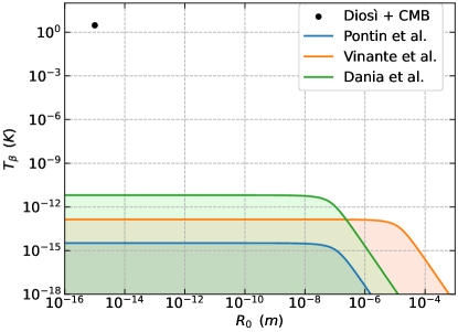
Figure 1: Experimental bounds for the dDP model. Blue, orange and green shaded areas represent the excluded values of the collapse parameters, respectively, from the experiments of Pontin et al., Vinante et al. and Dania et al.. The black point represents the proposal by Diósi of $R_{0}=10^{-15}$ m and $T_{\beta}\sim 3$ K being the CMB temperature.

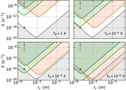
Figure 2: Experimental bounds for the dCSL model. Blue, orange and green shaded areas represent the excluded values of the collapse parameters, respectively, from the experiments of Pontin et al., Vinante et al. and Dania et al.. Each panel considers different values of $T_{\beta}$, left-to-right, top-to-bottom, these are 1 K, $10^{-4}$ K, $10^{-6}$ K and $10^{-9}$ K. The grey area is excluded for theoretical reasons Toroš et al. (2017). The grey bar is the Adler proposal of the CSL parameters Adler (2007) and the black point is the GRW proposal Ghirardi et al. (1986).

In Fig. 1 we show the excluded values of $T_{\beta}$ for the dDP model when varying $R_{0}$. For comparison, we also report (black dot) the values of Diósi proposal of $R_{0}=10^{-15}$ m matched with $T_{\beta}\sim 3$ K being the temperature of the cosmic microwave background (CMB). This choice is based on the hypothesis of a cosmological origin of the collapse mechanism, and thus one would expect a value of $T_{\beta}$ of this order of magnitude. We notice that below $T_{\beta}\sim 10^{-13}$ K and $T_{\beta}\sim 6\times 10^{-12}$ K all the values of $R_{0}$ respectively smaller than $10^{-6}$ m and $10^{-8}$ m are excluded, this includes the mesoscopic regime where one would expect a collapse.

In Fig. 2 we show the bounds on the dCSL parameters $\lambda$ and $r_{\text{\tiny C}}$ for four values of $T_{\beta}=1$ K, $10^{-3}$ K, $10^{-5}$ K and $10^{-7}$ K. The gray region is excluded theoretically as it would not guarantee an effective collapse of macroscopic quantum superpositions Toroš et al. (2017). The grey bar, which is the Adler proposal Adler (2007) for the CSL parameters, is excluded for each value of $T_{\beta}$ reported, while the GRW proposal Ghirardi et al. (1986) is excluded for $T_{\beta}=10^{-5}$ K and below. We notice that all the parameter space is excluded for temperatures lower than $6\times 10^{-9}$ K .

VI Comparison with the previous dissipative model

Here we compare the linear friction (LF) dissipative model, introduced in Ref. Di Bartolomeo et al. (2023) and shown in Eq. (1), with the previously proposed dissipative collapse models Smirne and Bassi (2015); Bahrami et al. (2014). The latter have a mathematical structure similar to the collisional dynamics of a test particle interacting with a low-density gas in the weak coupling regime Vacchini (2000). Thus, for simplicity, we refer to these as collisional dynamics (CD) models. For such a comparison, we compute the asymptotic temperature of the center of mass of the mechanical oscillator, which in both frameworks can be derived from their respective master equations. Indeed, given an arbitrary operator $\hat{O}$, one can compute the evolution of its expectation value as $\frac{\operatorname{d}\!}{\operatorname{d}\!t}\braket{\hat{O}}_{t}=\operatorname{Tr}(\hat{O}\frac{\operatorname{d}\!}{\operatorname{d}\!t}\hat{\rho}_{cm})$. The equation with $\hat{O}=\hat{H}$ is not in a closed form, however we can write the system of three differential equations for $\hat{O}=\hat{V}$, $\hat{K}$ and $\{\hat{x},\hat{p}\}$, where $\hat{K}=\hat{p}^{2}/2M$ and $\hat{V}=M\omega_{0}^{2}\hat{x}^{2}/2$. Under the assumption of a reaching a stable condition at the thermal equilibrium, we can set all the derivatives to zero and find the asymptotic values of $\braket{\hat{K}}_{\infty}$ and $\braket{\hat{V}}_{\infty}$, from which we obtain $\braket{\hat{H}}_{\infty}=\braket{\hat{K}}_{\infty}+\braket{\hat{V}}_{\infty}$. Then, we define the temperature of the system by exploiting the equipartition theorem for single harmonic oscillator $\braket{\hat{H}}_{\infty}=k_{\text{\tiny B}}T$.

In the LF framework, we have

$$\frac{\operatorname{d}\!\braket{\hat{V}}_{t}}{\operatorname{d}\!t} =-\Gamma\braket{\hat{V}}_{t}+\frac{\omega_{0}^{2}}{2}\braket{\{\hat{x},\hat{p}\}}_{t}+\frac{\Gamma^{2}M\omega_{0}^{2}}{8\eta},$$ (24)

$$\frac{\operatorname{d}\!\braket{\hat{K}}_{t}}{\operatorname{d}\!t} =-\Gamma\braket{\hat{K}}_{t}-\frac{\omega_{0}^{2}}{2}\braket{\{\hat{x},\hat{p}\}}_{t}+\frac{\hbar^{2}\eta}{2M},$$

$$\frac{\operatorname{d}\!\braket{\{\hat{x},\hat{p}\}}_{t}}{\operatorname{d}\!t} =-\Gamma\braket{\{\hat{x},\hat{p}\}}_{t}+4\braket{\hat{K}}_{t}-4\braket{\hat{V}}_{t},$$

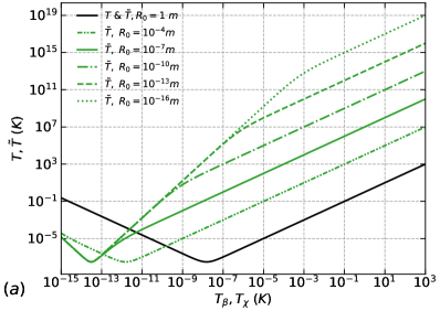
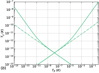
Figure 3: Comparison between the linear friction dDP and the collisional dynamics dDP models. In panel (a) the solid black curve represents the asymptotic temperature $T$ of the LF-dDP model as a function of the dissipation parameter $T_{\beta}$, while the green curves show the asymptotic temperature $\tilde{T}$ of the CD-dDP model as a function of the dissipation parameter $T_{\chi}$ for different values of $R_{0}$. For $R_{0}=1$ m, $T$ and $\tilde{T}$ coincide in the black curve. Panel (b) shows the contour plot of the function $T(T_{\beta})-\tilde{T}(T_{\chi})=0$ where the solid green line is for $R_{0}=10^{-7}$ m and the dash dotted green line is for $R_{0}=10^{-10}$ m.

which correspond to

$$T=T_{\beta}+\frac{\hbar^{2}\omega_{0}^{2}}{16k_{\text{\tiny B}}^{2}T_{\beta}},$$ (25)

both for the dDP and the dCSL model. We notice that Eq. (25) does not depend on the free parameters of the model except for the dissipation parameter $\beta=(k_{\text{\tiny B}}T_{\beta})^{-1}$. When $T_{\beta}$ is high, the asymptotic temperature $T$ coincides with the collapse temperature $T_{\beta}$. Indeed, in the limit of $T_{\beta}\to\infty$ ($\beta\to 0$, i.e. $\Gamma\to 0$), the last term of the first expression in Eq. (24) can be neglected and the only important collapse term is the last one in the second expression. In such a way one recovers the predictions of the standard collapse model without dissipation, for which one has $T=\infty$. Also in the limit of $T_{\beta}\to 0$, the asymptotic temperature $T$ goes to infinity. Indeed, in such a limit, is the last term in the second expression of Eq. (24) that can be neglected, and the last term in the first expression becomes the relevant one. The latter leads to an infinite increase to the mean potential energy, and thus to $\braket{\hat{H}}_{\infty}=\infty$.

In the CD framework, one has

$$\frac{\operatorname{d}\!\braket{\hat{V}}_{t}}{\operatorname{d}\!t} =\frac{\omega_{0}^{2}}{2}\braket{\{\hat{x},\hat{p}\}}_{t}+\frac{\tilde{\Gamma}^{2}M\omega_{0}^{2}}{8\tilde{\eta}},$$ (26)

$$\frac{\operatorname{d}\!\braket{\hat{K}}_{t}}{\operatorname{d}\!t} =-2\tilde{\Gamma}\braket{\hat{K}}_{t}-\frac{\omega_{0}^{2}}{2}\braket{\{\hat{x},\hat{p}\}}_{t}+\frac{\hbar^{2}\tilde{\eta}}{2M},$$

$$\frac{\operatorname{d}\!\braket{\{\hat{x},\hat{p}\}}_{t}}{\operatorname{d}\!t} =-\tilde{\Gamma}\braket{\{\hat{x},\hat{p}\}}_{t}+4\braket{\hat{K}}_{t}-4\braket{\hat{V}}_{t},$$

whose corresponding asymptotic temperature reads

$$\tilde{T}=\frac{\tilde{\Gamma}M\omega_{0}^{2}}{8\tilde{\eta}k_{\text{\tiny B}}}+\frac{\hbar^{2}\tilde{\eta}}{2M\tilde{\Gamma}k_{\text{\tiny B}}}+\frac{\tilde{\Gamma}^{3}M}{16\tilde{\eta}k_{\text{\tiny B}}}.$$ (27)

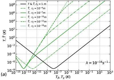
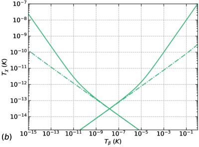
Figure 4: Comparison between the linear friction dCSL and the collisional dynamics dCSL models. In panel (a) the solid black curve represents the asymptotic temperature $T$ of the LF-dCSL model as a function of the dissipation parameter $T_{\beta}$, while the green curves show the asymptotic temperature $\tilde{T}$ of the CD-dCSL model as a function of the dissipation parameter $T_{\chi}$ for different values of $r_{\text{\tiny C}}$. For $r_{\text{\tiny C}}=1$ m, $T$ and $\tilde{T}$ coincide in the black curve. Panel (b) shows the contour plot of the function $T(T_{\beta})-\tilde{T}(T_{\chi})=0$ where the solid green line is for $r_{\text{\tiny C}}=10^{-7}$ m and the dash dotted green line is for $r_{\text{\tiny C}}=10^{-10}$ m. We fix $\lambda=10^{-16}$ s^-1.

The latter depends on two parameters $\tilde{\eta}$ and $\tilde{\Gamma}$ that play the role, respectively, of $\eta$ and $\Gamma$ in the LF framework Nobakht et al. (2018). To be specific, we have $\tilde{\Gamma}=4\tilde{\eta}\sigma^{2}\chi(1+\chi)m_{0}/M$ with $\sigma=R_{0}$ or $r_{\text{\tiny C}}$ and where $\chi=\hbar^{2}/8m_{0}\sigma k_{\text{\tiny B}}T_{\chi}$ is the dissipation parameter of the CD model and $T_{\chi}$ is the associated temperature of the collapse field (analogous to $T_{\beta}$ in the LF framework). The coefficient $\tilde{\eta}$ takes the following form

$$\tilde{\eta}_{\text{DP}}=\sqrt{\pi}\operatorname{erf}\left(\frac{r}{\tilde{R}_{0}}\right)+\frac{GM^{2}R_{0}}{\sqrt{\pi}r^{3}}\Biggl{[}\frac{R_{1}}{r}\left(e^{-\frac{r^{2}}{R_{1}^{2}}}-3\right)+2\frac{R_{1}^{3}}{r^{3}}\left(1-e^{-\frac{r^{2}}{R_{1}^{2}}}\right)\Biggr{]},$$ (28)

for the CD-dDP model with $R_{1}=R_{0}(1+\chi)$, and

$$\tilde{\eta}_{\text{CSL}}=\frac{3\lambda M^{2}r_{\text{\tiny C}}^{3}}{R_{\text{\tiny C}}m_{0}^{2}r^{4}}\Biggl{[}1-2\left(\frac{R_{\text{\tiny C}}}{r}\right)^{2}+e^{-\frac{r^{2}}{R_{\text{\tiny C}}^{2}}}\left(1+2\frac{R_{\text{\tiny C}}^{2}}{r^{2}}\right)\Biggr{]},$$ (29)

for the CD-dCSL model with $R_{\text{\tiny C}}=r_{\text{\tiny C}}(1+\chi)$. Notably, in the CD framework, $\tilde{T}$ depends on all the free parameters of the CD model. In the limit $T_{\chi}\to\infty$ ($\chi\to 0$), one recovers the standard collapse model with $\tilde{T}=\infty$. In the opposite limit, for $T_{\chi}\to 0$ (i.e. $\tilde{\Gamma}\to\infty$), the last term of the first expression of Eq. (26) is the relevant one, while the last of the second expression can be neglected. Then, following the same reasoning as in the LF framework, one has $\tilde{T}=\infty$.

In Fig. 3 we compare LF-dDP and CD-dDP models, where the experimental values considered are the mass and the radius of the nano-particle from Dania et al. Dania et al. (2023). In panel (a) we show in black the plot of $T$ as a function of $T_{\beta}$ and in green the plots of $\tilde{T}$ as a function of $T_{\chi}$ for various values of $R_{0}$. We notice that $T$ and $\tilde{T}$ coincide for $R_{0}=1$ m. As $R_{0}$ decreases, the difference between $T$ and $\tilde{T}$ increases.

More interestingly if we assume that both the models reach the same asymptotic temperature, namely $T=\tilde{T}$, then we can link the two dissipation parameters $T_{\beta}$ and $T_{\chi}$ and display how they are related. Thus, in panel (b) of Fig. 3 we show the plot of the function $T(T_{\beta})-\tilde{T}(T_{\chi})=0$. The solid green line is for $R_{0}=10^{-7}$ m and the dash dotted one for $R_{0}=10^{-10}$ m. In general the relation between $T_{\beta}$ and $T_{\chi}$ is non-linear and it does not lead to a one-to-one relation. However, in some regimes, we have a linear behaviour and we can compare the two collapse temperatures $T_{\beta}$ and $T_{\chi}$ directly. For example $T_{\beta}=1$ K corresponds to $T_{\chi}=10^{-7}$ K for $R_{0}=10^{-7}$ m (solid line) and to $T_{\chi}\sim 10^{-10}$ K for $R_{0}=10^{-10}$ m (dashed line).

We show the same analysis for LF-dCSL and CD-dCSL models in Fig. 4 where we used the same colouring and dashing as in Fig. 3, and where we set $\lambda=10^{-16}$ s^-1 corresponding to the GRW point at $r_{\text{\tiny C}}=10^{-7}$ m. We notice that the LF-dCSL and CD-dCSL models lead two different predictions. This is exemplified by the GRW point, which in the CD-dCSL model is excluded for collapse temperatures $T_{\chi}$ below $10^{-9}$ K (see Ref. Vinante et al. (2020b)). On the other hand, focusing on the top right branch of the solid line in Fig. 4b, the value of $T_{\chi}=10^{-9}$ K corresponds to $T_{\beta}=10^{-2}$ K for which the GRW point is not excluded [cf. Fig. 2]. This means that the two frameworks, LF and CD, can be in principle discriminates experimentally. A similar example can be showcased in the comparison of the LF-dDP and CD-dDP models. Notably, the relation between $T_{\chi}$ and $T_{\beta}$ for the dDP and dCSL models show the same behaviour [cf. Fig. 3b and Fig. 4b].

VII Conclusions and Outlook

A new mechanism to introduce dissipation in collapse models has been recently proposed. Conversely to a previously proposed one, this mechanism is based on the a friction being linear in the current in a many-body system. This approach, which has not yet been tested, opens a promising avenue for new investigations in the collapse models framework. We focus on establishing the first experimental bounds for linear-friction dissipative DP (dDP) and CSL (dCSL) models, using data from levitated optomechanical experiments. The results reveal significant exclusions of the parameter space, with collapse temperatures below $T_{\beta}\sim 10^{-13}$ K and $T_{\beta}\sim 6\times 10^{-12}$ K for dDP model and all parameter space for dCSL model is excluded for temperatures below $T_{\beta}\sim 6\times 10^{-9}$ K. Finally, we compare the linear friction dissipative models with those previously introduced, which we refer to as collisional dynamics dissipative models. We find the relations between the respective collapse temperature under the assumption that the collapse process leads the system to thermalisation. We conclude that they can in principle be discriminated experimentally.

References

• Bassi and Ghirardi (2003) A. Bassi and G. Ghirardi, Physics Reports 379, 257 (2003).
• Bassi et al. (2013) A. Bassi, K. Lochan, S. Satin, T. P. Singh, and H. Ulbricht, Reviews of Modern Physics 85, 471 (2013).
• Carlesso et al. (2022) M. Carlesso, S. Donadi, L. Ferialdi, M. Paternostro, H. Ulbricht, and A. Bassi, Nature Physics 18, 243 (2022).
• Diosi (1987) L. Diosi, Physics Letters A 120, 377 (1987).
• Penrose (1996) R. Penrose, General relativity and gravitation 28, 581 (1996).
• Pearle (1989) P. Pearle, Physical Review A 39, 2277 (1989).
• Ghirardi et al. (1990) G. C. Ghirardi, P. Pearle, and A. Rimini, Physical Review A 42, 78 (1990).
• Bilardello et al. (2016) M. Bilardello, S. Donadi, A. Vinante, and A. Bassi, Physica A 462, 764 (2016).
• Vinante et al. (2016) A. Vinante, M. Bahrami, A. Bassi, O. Usenko, G. Wijts, and T. Oosterkamp, Physical review letters 116, 090402 (2016).
• Carlesso et al. (2016) M. Carlesso, A. Bassi, P. Falferi, and A. Vinante, Phys. Rev. D 94, 124036 (2016).
• Adler et al. (2019) S. L. Adler, A. Bassi, M. Carlesso, and A. Vinante, Phys. Rev. D 99, 103001 (2019).
• Vinante et al. (2017) A. Vinante, R. Mezzena, P. Falferi, M. Carlesso, and A. Bassi, Physical review letters 119, 110401 (2017).
• Helou et al. (2017) B. Helou, B. Slagmolen, D. E. McClelland, and Y. Chen, Physical Review D 95, 084054 (2017).
• Vinante et al. (2020a) A. Vinante, M. Carlesso, A. Bassi, A. Chiasera, S. Varas, P. Falferi, B. Margesin, R. Mezzena, and H. Ulbricht, Phys. Rev. Lett. 125, 100404 (2020a).
• Zheng et al. (2020) D. Zheng, Y. Leng, X. Kong, R. Li, Z. Wang, X. Luo, J. Zhao, C.-K. Duan, P. Huang, J. Du, M. Carlesso, and A. Bassi, Phys. Rev. Res. 2, 013057 (2020).
• Pontin et al. (2020) A. Pontin, N. P. Bullier, M. Toroš, and P. F. Barker, Phys. Rev. Res. 2, 023349 (2020).
• Donadi et al. (2021a) S. Donadi, K. Piscicchia, R. Del Grande, C. Curceanu, M. Laubenstein, and A. Bassi, The European Physical Journal C 81, 1 (2021a).
• Donadi et al. (2021b) S. Donadi, K. Piscicchia, C. Curceanu, L. Diósi, M. Laubenstein, and A. Bassi, Nature Physics 17, 74 (2021b).
• Arnquist et al. (2022) I. J. Arnquist et al. (Majorana Collaboration), Phys. Rev. Lett. 129, 080401 (2022).
• Smirne and Bassi (2015) A. Smirne and A. Bassi, Scientific reports 5, 1 (2015).
• Bahrami et al. (2014) M. Bahrami, A. Smirne, and A. Bassi, Physical Review A 90, 062105 (2014).
• Nobakht et al. (2018) J. Nobakht, M. Carlesso, S. Donadi, M. Paternostro, and A. Bassi, Physical Review A 98, 042109 (2018).
• Vinante et al. (2019) A. Vinante, A. Pontin, M. Rashid, M. Toroš, P. Barker, and H. Ulbricht, Physical Review A 100, 012119 (2019).
• Di Bartolomeo et al. (2023) G. Di Bartolomeo, M. Carlesso, K. Piscicchia, C. Curceanu, M. Derakhshani, and L. Diósi, Phys. Rev. A 108, 012202 (2023).
• Dania et al. (2023) L. Dania, D. S. Bykov, F. Goschin, M. Teller, and T. E. Northup, arXiv preprint arXiv:2304.02408  (2023).
• Di Bartolomeo et al. (2021) G. Di Bartolomeo, M. Carlesso, and A. Bassi, Phys. Rev. D 104, 104027 (2021).
• Mancini and Tombesi (1994) S. Mancini and P. Tombesi, Physical Review A 49, 4055 (1994).
• Gardiner and Zoller (2004) C. Gardiner and P. Zoller, Quantum Noise (Springer-Verlag Berlin, 2004).
• Paternostro et al. (2006) M. Paternostro, S. Gigan, M. S. Kim, F. Blaser, H. Böhm, and M. Aspelmeyer, New Journal of Physics 8, 107 (2006).
• Millen et al. (2020) J. Millen, T. S. Monteiro, R. Pettit, and A. N. Vamivakas, Reports on Progress in Physics 83, 026401 (2020).
• Gonzalez-Ballestero et al. (2021) C. Gonzalez-Ballestero, M. Aspelmeyer, L. Novotny, R. Quidant, and O. Romero-Isart, Science 374, eabg3027 (2021).
• Moore and Geraci (2021) D. C. Moore and A. A. Geraci, Quantum Science and Technology 6, 014008 (2021).
• Vinante et al. (2020b) A. Vinante, G. Gasbarri, C. Timberlake, M. Toroš, and H. Ulbricht, Physical Review Research 2, 043229 (2020b).
• Toroš et al. (2017) M. Toroš, G. Gasbarri, and A. Bassi, Physics Letters A 381, 3921 (2017).
• Adler (2007) S. L. Adler, Journal of Physics A: Mathematical and Theoretical 40, 2935 (2007).
• Ghirardi et al. (1986) G. C. Ghirardi, A. Rimini, and T. Weber, Physical review D 34, 470 (1986).
• Vacchini (2000) B. Vacchini, Physical Review Letters 84, 1374 (2000).