Distributed Data-driven Unknown-input Observers

Abstract

Unknown inputs related to, e.g., sensor aging, modeling errors, or device bias, represent a major concern in wireless sensor networks, as they degrade the state estimation performance. To improve the performance, unknown-input observers (UIOs) have been proposed. Most of the results available to design UIOs are based on explicit system models, which can be difficult or impossible to obtain in real-world applications. Data-driven techniques, on the other hand, have become a viable alternative for the design and analysis of unknown systems using only data. In this context, a novel data-driven distributed unknown-input observer (D-DUIO) for an unknown linear system is developed, which leverages solely some data collected offline, without any prior knowledge of the system matrices. In the paper, first, the design of a DUIO is investigated by resorting to a traditional model-based approach. By resorting to a Lyapunov equation, it is proved that under some conditions, the state estimates at all nodes of the DUIO achieve consensus and collectively converge to the state of the system. Moving to a data-driven approach, it is shown that the input/output/state trajectories of the system are compatible with the equations of a D-DUIO, and this allows, under suitable assumptions, to express the matrices of a possible DUIO in terms of the matrices of pre-collected data. Then, necessary and sufficient conditions for the existence of the proposed D-DUIO are given. Finally, the efficacy of the D-DUIO is illustrated by means of numerical examples.

I Introduction

In dynamical control systems, state estimation plays a vital role, and a multitude of well-established tools have been developed, including the celebrated Kalman filter and Luenberger observer [1, 2, 3]. Many efforts have focused on the design and performance analysis of centralized state estimators, which compute the system state in a centralized manner by collecting, transmitting, and fusing all sensor measurements [4]. However, in networked control systems, cyber-physical systems, and the internet of things, the system of interest may be too large or exhibit a too complex connection structure for centralized state estimation schemes to be effective, given the limited communication bandwidth, computing resources, and time budget.

Distributed state estimation (DSE) approaches have gained attention thanks to recent advances in micro-computing devices and telecommunication technologies. These methods perform local estimation of the system state based on locally available sensor measurements, plus additional information received from neighboring agents or subsystems. DSE has a wide range of real-world applications, including power system monitoring, cooperative tracking and localization, and smart transportation; see, e.g., [4, 5, 6] and references therein. Several DSE methods have been developed, such as consensus Kalman-based filtering [4, 7, 8, 9], Luenberger-like consensus estimation [10], and distributed moving-horizon estimation [11], to name a few.

One of the most popular DSE methods is the distributed Kalman filtering (DKF) algorithm, which was pioneered by [4]. A Kalman consensus filtering approach (KCF) was proposed in [12] to reduce the disagreement of state estimates between different nodes. Its formal derivation, stability, and performance analysis were studied in [13]. An information-weighting mechanism was introduced into KCF in [14] to deal with the inaccurate estimation performance caused by naive nodes. A networked measurement model consisting of both direct and indirect target state measurements was employed to derive locally optimal state estimates, based on the information-weighted KCF in [15].

However, practical concerns about the deployment of DSE methods exist. For instance, unknown inputs caused by sensor aging, modeling errors, calibration bias, and/or external disturbances/attacks can lead to severe deterioration in estimation performance [16, 17]. Among different tools to tackle the estimation problem in the presence of unknown inputs, unknown-input observers (UIOs) have attracted recurring attention due to their geometric decoupling capabilities [18, 19]. A distributed dynamic estimator was designed to simultaneously estimate the state and the unknown input in [20]. A distributed UIO (DUIO) was first implemented in [21], to estimate the internal states of the nonlinear subsystems using local measurement outputs. A finite-frequency $H_{\infty}$-UIO, considering information exchanges between neighbors in a multi-agent system setting, was studied for distributed fault estimation in [22]. More recently, a distributed UIO was developed in [23] by resorting to a consensus strategy, in which the global system state is estimated consistently by each local observer with limited information about the input and output.

It is worth noting that all of the previous results about DUIOs were derived assuming that the original system models were known. However, obtaining accurate system models for interconnected cyber-physical systems from first-principles or through system identification methods is becoming increasingly difficult or even impossible. To address this challenge, data-driven control methods have gained attention in the big data era, aiming to design controllers directly from data without relying on intermediate system identification procedures, as described in [24, 25]. Recent efforts leveraging Willems et al.’s fundamental lemma [26] have addressed data-driven state feedback control [27, 28], data-driven predictive control [29, 30], data-driven event-triggered and consensus control [31, 32, 33]. However, data-driven state estimation has received only partial attention up to now. In [34], a robust data-driven moving horizon estimation scheme was developed using offline input/output/state data. The work [35] investigated the data-driven UIO problem for unknown linear systems, with the goal of estimating the state even in the presence of unknown disturbances. This work was recently extended in [36], where weaker conditions for the problem solution were provided, together with a complete analysis of the equivalence between the model-based and the data-driven approaches to the problem solution. Nevertheless, all these studies have only considered centralized systems, and to the best of our knowledge, no results for data-driven DSE have been reported.

This paper aims to fill this gap by developing a distributed data-driven UIO scheme for unknown linear systems subject to unknown inputs and disturbances.

In real-world applications, communication channels in sensor networks are subject to multipath, fading, and dropout. Such limitations may ultimately lead to poor state estimation performance at a node. To compensate for this, cooperative state estimation methods are used for real-time state estimation. The key of cooperative state estimation is to reduce the disagreement between local state estimators. Consensus protocols have proven to be effective tools for disagreement reduction and are widely used for distributed computing over sensor networks [12] and [13]. Inspired by [12] and [23], we propose a D-DUIO framework with a consensus strategy to enhance the estimation performance. Specifically, we introduce a novel data-driven distributed UIO (D-DUIO) designed using offline input/output/state data without performing any system identification. The D-DUIO allows the estimation of the unknown global system state through local information exchanges between neighboring nodes, even when no node has access to the complete input information. It is shown that, under mild conditions, the local state estimates obtained by the nodes reach consensus and converge to the true state of the unknown system.

In summary, the contributions of this work are the following:

• By resorting to a standard model-based approach, we establish necessary and sufficient conditions for the proposed DUIO to provide a state estimate that asymptotically converges to the true state of the system.

• We develop a data-driven counterpart of the same DUIO, based on the DUIO in [23] and the data-driven UIO in [35].

• We prove that, under mild assumptions, the data-driven DUIO estimates the system state with an error that asymptotically converges to zero. In addition, we also show that the conditions obtained in the data-driven framework actually coincide with the ones provided by the standard model-based approach.

The rest of the paper is organized as follows. In Section II, the preliminaries and the problem formulation are introduced. Section III describes the structure of the proposed DUIO and discusses its existence, as well as the estimation error convergence, using a model-based approach. In Section IV the same analysis is carried out in a data-driven framework. A numerical example is provided in Section V, and concluding remarks are drawn in Section VI.

For convenience, we introduce some notation. The sets of real numbers, nonnegative real numbers and nonnegative integers are denoted by $\mathbb{R},{\mathbb{R}}_{+},$ and $\mathbb{Z}_{+}$, respectively. The identity matrix, zero matrix and all-one vector are denoted by $I$, $\mathbf{0}$ and ${\mathbb{1}}$, respectively, the dimensions being clear from the context. The pseudo-inverse of a matrix $Q$ is denoted by $Q^{\dagger}$. We use $\ker(Q)$ to represent the kernel space of $Q$ and ${\rm range}(Q)$ to represent its column space. The spectrum of a square matrix $Q$ is denoted by $\sigma(Q)$ and is the set of all its eigenvalues. For a symmetric matrix $Q$, we use $\bar{\lambda}(Q)(\underline{\lambda}(Q))$ and $\lambda_{2}(Q)$ to denote the largest (smallest) and the second smallest eigenvalues of $Q$, respectively. Given a symmetric matrix $Q$, $Q>{\bf 0}$ ($Q\geq{\bf 0}$) means that $Q$ is positive definite (semidefinite). Analogous symbols are used to denote that $Q$ is negative definite (semidefinite).
The Kronecker product is denoted by $\otimes$. Given matrices $M_{i},i\in\{1,2,\dots,p\}$, the block-diagonal matrix whose $i$th diagonal block is the matrix $M_{i}$ is denoted by ${\rm diag}(M_{i})$. Given a sequence of matrices with the same number of columns (in particular, vectors) $\{M(k)\}_{k=0}^{N-1}$, we denote by ${\rm col}(\{M(k)\}_{k=0}^{N-1})$ the matrix obtained by column concatenation of the matrices $M(k)$. The Hankel matrix of depth $L\in\mathbb{Z}_{+}$ associated with the vector sequence $\{f(k)\}_{k=0}^{N-1}$ (in the following denoted by $f$, for the sake of brevity) is

$${\mathcal{H}}_{L}(f):=\left[\begin{matrix}f(0)&f(1)&\cdots&f(N-L)\\ f(1)&f(2)&\cdots&f(N-L+1)\\ \vdots&\vdots&\ddots&\vdots\\ f(L-1)&f(L)&\cdots&f(N-1)\\ \end{matrix}\right].$$

The definition of persistency of excitation (see [26, Section 3]) is given below.

Definition 1 (Persistency of excitation).

A sequence $f=\{f(k)\}_{k=0}^{N-1}$ is persistently exciting of order $L$, if ${\mathcal{H}}_{L}(f)$ has full row rank.

II Preliminaries and Problem Formulation

Consider the following discrete-time linear system

$$x(k+1)=Ax(k)+Bu(k)+Ed(k)$$ (1)

where $k\in{\mathbb{Z}}_{+}$, $x(k)\in\mathbb{R}^{n_{x}}$ is the state, $u(k)\in\mathbb{R}^{n_{u}}$ is the control input, $d(k)\in\mathbb{R}^{n_{d}}$ is the unknown process disturbance, $A\in\mathbb{R}^{n_{x}\times n_{x}}$, $B\in\mathbb{R}^{n_{x}\times n_{u}}$, and $E\in\mathbb{R}^{n_{x}\times n_{d}}$.

A wireless sensor network comprising $M$ homogeneous sensor nodes is deployed to monitor the state of system (1). At each time instant, each node of the network provides an output signal, which is a noisy measurement of a linear function of the system state, given by

$$y_{i}(k)=C_{i}x(k)+D_{i}v_{i}(k),\quad\forall i\in\mathcal{M}:=\{1,2,\ldots,M\},$$ (2)

where $y_{i}(k)\in\mathbb{R}^{n_{y_{i}}}$ and $v_{i}(k)\in\mathbb{R}^{n_{v_{i}}}$ denote the measured output and unknown measurement noise, respectively, $C_{i}\in\mathbb{R}^{n_{y_{i}}\times n_{x}}$ and $D_{i}\in\mathbb{R}^{n_{y_{i}}\times n_{v_{i}}}$. Moreover, we assume that each sensor node has access only to a subset of the input entries, and hence for every $i\in\mathcal{M}$, we can split the entries of the control input $u(k)$ into two parts: the measurable part $u_{i}(k)$ and the unknown part $u_{i}^{u}(k)$. Consequently, we can always express $Bu(k)$ as:

$$Bu(k)=B^{m}_{i}u_{i}(k)+B^{u}_{i}u_{i}^{u}(k),$$ (3)

where $u_{i}(k)\in{\mathbb{R}}^{n_{m_{i}}}$, $B^{m}_{i}\in{\mathbb{R}}^{n_{x}\times n_{m_{i}}}$, $u_{i}^{u}(k)\in{\mathbb{R}}^{n_{p_{i}}}$, $B^{u}_{i}\in{\mathbb{R}}^{n_{x}\times n_{p_{i}}}$. Since $d(k)$ is also unknown for each node, the overall unknown input at node $i$ and the associated system matrix can be represented as

$$w_{i}(k) :=\big{[}(u_{i}^{u}(k))^{\top}\ d^{\top}(k)\big{]}^{\top},$$ (4a)

$$B_{i}^{p} :=[B^{u}_{i}\ E].$$ (4b)

Consequently, for every $i\in\mathcal{M}$, the system dynamics, from the perspective of the $i$th sensor node, is given by:

$$x(k+1)=Ax(k)+B_{i}^{m}u_{i}(k)+B_{i}^{p}w_{i}(k).$$ (5)

In the following, we will denote by ${\mathcal{T}}_{i}$ the system described by the pair of equations (1)–(2) or, equivalently, by the pair (5)–(2).

Throughout this paper, we make the following assumptions on the systems ${\mathcal{T}}_{i},i\in{\mathcal{M}}$.

Assumption 1 (Unknown system model).

For each $i\in\mathcal{M}$, the matrices $(A,B,E,C_{i},D_{i})$ of the system ${\mathcal{T}}_{i}$ are unknown, but it is known which input signals are measurable, namely which entries of $u$ constitute $u_{i}$.

Assumption 2 (Detectability).

For every $i\in{\mathcal{M}}$, the pair $(C_{i},A)$ is detectable.

In industrial processes, it is not always feasible or safe to measure real-time states and transmit them to remote sensors. However, offline experiments can be conducted to gather state data. Such data are sent to the sensors to design state observers that will subsequently operate online. In line with recent studies [30, 37, 31, 35, 33], we assume that input/output/state data can be locally and independently collected at each node of system ${\mathcal{T}}_{i}$ through equations (1)–(2) using different sensors. We make the following assumption on data acquisition.

Assumption 3 (Offline and online data acquisition).

During the offline phase, input/output/state data $\bar{u}_{i}:={\rm col}(\{\bar{u}_{i}(k)\}_{k=0}^{N-1})$, $\bar{y}_{i}:={\rm col}(\{\bar{y}_{i}(k)\}_{k=0}^{N-1})$ and $\bar{x}_{i}:={\rm col}(\{\bar{x}_{i}(k)\}_{k=0}^{N-1})$ are collected locally by each system ${\mathcal{T}}_{i}$ described as in (1)–(2), possibly corresponding to different initial states and inputs. During online operations, only the measurable inputs $u_{i}(k)$ and outputs $y_{i}(k),i\in{\mathcal{M}},$ are available.

Under Assumption 3, we define for every $i\in{\mathcal{M}}$ Hankel matrices of depth $L=2$ as follows: $U_{i}:={\mathcal{H}}_{2}(\bar{u}_{i})\in{\mathbb{R}}^{2{n_{m_{i}}}\times(N-1)}$, $Y_{i}:={\mathcal{H}}_{2}(\bar{y}_{i})\in{\mathbb{R}}^{2{n_{y_{i}}}\times(N-1)}$, and $X_{i}:={\mathcal{H}}_{2}(\bar{x}_{i})\in{\mathbb{R}}^{2{n_{x}}\times(N-1)}$. We partition the rows of each such matrix into a past and a future block of equal sizes, denoted by $p$ and $f$, respectively:

$$U_{i}=\begin{bmatrix}U_{i}(p)\\ U_{i}(f)\end{bmatrix},\ Y_{i}=\begin{bmatrix}Y_{i}(p)\\ Y_{i}(f)\end{bmatrix},\ X_{i}=\begin{bmatrix}X_{i}(p)\\ X_{i}(f)\end{bmatrix}.$$ (6)

In addition, we introduce the notation $\bar{w}_{i}:={\rm col}(\{\bar{w}_{i}(k)\}_{k=0}^{N-1})$ and $\bar{v}_{i}:={\rm col}(\{\bar{v}_{i}(k)\}_{k=0}^{N-1})$ to represent the unknown input and the measurement noise sequences, respectively, during the offline data collection process. The corresponding Hankel matrices are

$$W_{i}:={\mathcal{H}}_{2}(\bar{w}_{i})=\begin{bmatrix}W_{i}(p)\\ W_{i}(f)\end{bmatrix},V_{i}:={\mathcal{H}}_{2}(\bar{v}_{i})=\begin{bmatrix}V_{i}(p)\\ V_{i}(f)\end{bmatrix}$$

where $W_{i}\in{\mathbb{R}}^{2({n_{p_{i}}+n_{d}})\times(N-1)}$ and $V_{i}\in{\mathbb{R}}^{2{n_{v_{i}}}\times(N-1)}$.

We make the following assumption on the pre-collected data.

Assumption 4 (Rank of pre-collected data).

For each $i\in\mathcal{M}$, it holds that

$${\rm rank}\!\left(\begin{bmatrix}U_{i}(p)\\ W_{i}(p)\\ X_{i}(p)\\ V_{i}\\ \end{bmatrix}\right)=n_{m_{i}}+n_{p_{i}}+n_{d}+n_{x}+2n_{v_{i}}.$$

Remark 1.

As it will be proved in the following, Assumption 4 ensures that any input/output/state trajectory of system ${\mathcal{T}}_{i}$ can be represented as a linear combination of the columns of $[U_{i}^{\top}(p)\ X_{i}^{\top}\ Y_{i}^{\top}]^{\top}$. This implies that $[U_{i}^{\top}(p)\ X_{i}^{\top}\ Y_{i}^{\top}]^{\top}$ encodes full information about the dynamics of the system. If the pair $(A,B)$ is controllable then, according to Willem’s Fundamental Lemma [26], this assumption is fulfilled when $\{[u_{i}^{\top}(k)\ w_{i}^{\top}(k)\ v_{i}^{\top}(k)]^{\top}\}_{k=0}^{N-1}$ is persistently exciting of order $n_{x}+2$. So, Assumption 4 is not overly conservative (see [30, 35, 33]).

The sensor network is represented by a graph $\mathcal{G}=(\mathcal{M},\mathcal{E},\mathcal{A})$, where $\mathcal{M}=\{1,2,\dots,M\}$ is the set of sensor nodes, $\mathcal{E}\subseteq\mathcal{M}\times\mathcal{M}$ is the set of communication links, through which nodes can exchange information, and $\mathcal{A}=[a_{ij}]\in\mathbb{R}_{+}^{M\times M}$ is the nonnegative weighted adjacency matrix where $a_{ij}=1$ if $(j,i)\in\mathcal{E}$, and $a_{ij}=0$ otherwise. The degree matrix of $\mathcal{G}$ is $\mathcal{D}={\rm diag}(r_{i})\in\mathbb{R}^{M\times M}$, where $r_{i}=\sum_{j=1}^{M}a_{ij}$, for every $i\in\mathcal{M}$. The Laplacian matrix associated with the network is $\mathcal{L}=\mathcal{D}-\mathcal{A}$.

Assumption 5 (Communication network).

The graph $\mathcal{G}$ is undirected and connected.

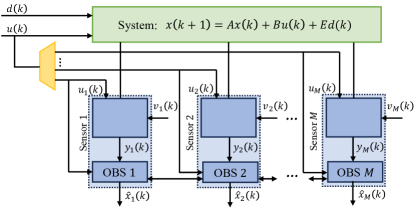
Figure 1: Scheme of the proposed distributed sensor network.

A distributed sensor network is represented in Fig. 1, to illustrate the proposed architecture.

In the proposed set-up and under the previous assumptions, we provide a first qualitative statement of the estimation problem we address in the paper.

Problem 1.

Given the unknown systems ${\mathcal{T}}_{i}$, $i\in\mathcal{M}$, subject to unknown inputs and disturbances, and satisfying Assumptions 1—5, design a distributed state estimation scheme whose description is based on the collected offline data, such that the state estimates provided by the observers across all nodes achieve consensus and the common state estimate converges to the real state value.

III Distributed Model-based State Estimation

If all the system matrices $(A,B,E,C_{i},D_{i})$, $i\in{\mathcal{M}},$ are known (which amounts to saying that only Assumptions 2 and 5 are preserved), the DUIO problem can be solved by means of a model-based approach that we briefly review here, similarly to what has been done for instance in [23] (see Remark 2 for a comparison).

In the model-based DUIO, neighboring nodes can exchange local state estimates to generate a consensus estimate of the system state $x$ using a recursive algorithm. Specifically, the $i$th sensor node generates the state estimate at time $k$, $\hat{x}_{i}(k)$, through the observer equations:

$${\rm DUIO}\!\left\{\begin{array}[]{l}\begin{aligned} z_{i}(k+1)&=E_{i}z_{i}(k)+F_{i}u_{i}(k)+L_{i}y_{i}(k)\\ &\quad+\chi P_{i}^{-1}\sum\limits_{j=1}^{M}a_{ij}[\hat{x}_{j}(k)-\hat{x}_{i}(k)]\\ \hat{x}_{i}(k)&=z_{i}(k)+H_{i}y_{i}(k)\end{aligned}\end{array}\right.$$ (7)

where $z_{i}(k)\in\mathbb{R}^{n_{x}}$ is the state of the $i$th DUIO, $\hat{x}_{i}(k)$ is the estimate of system (1) state provided by node $i$, $E_{i}\in\mathbb{R}^{n_{x}\times n_{x}}$, $F_{i}\in\mathbb{R}^{n_{x}\times n_{m_{i}}}$, $L_{i},H_{i}\in\mathbb{R}^{n_{x}\times n_{y_{i}}}$, $P_{i}\in\mathbb{R}^{n_{x}\times n_{x}}$ is a positive definite matrix, and $\chi$ a parameter to be designed. Finally, the $a_{ij}$’s are the (known) entries of the adjacency matrix $\mathcal{A}\in{\mathbb{R}}_{+}^{M\times M}$. Note that the consensus term is meant to improve accuracy (see, e.g., [12, Algorithm 2]).

Upon introducing the estimation error $e_{i}(k):=x(k)-\hat{x}_{i}(k)$ of node $i$, similarly to [18, Sections 2–3] and [23, Section 4], one deduces that the $i$th estimation error dynamics is

$$\!\!e_{i}(k+1)=x(k+1)-\hat{x}_{i}(k+1)$$ (8)

$$= \!\!x(k+1)-z_{i}(k+1)-H_{i}y_{i}(k+1)$$

$$= \!\!x(k+1)-E_{i}z_{i}(k)-F_{i}u_{i}(k)-L_{i}y_{i}(k)$$

$$\!\!-\chi P_{i}^{-1}\sum\limits_{j=1}^{M}a_{ij}[\hat{x}_{j}(k)-\hat{x}_{i}(k)]-H_{i}y_{i}(k+1)$$

$$= \!\!x(k+1)-E_{i}\hat{x}_{i}(k)+E_{i}H_{i}(C_{i}x(k)+D_{i}v_{i}(k))$$

$$\!\!-F_{i}u_{i}(k)-L_{i}(C_{i}x(k)+D_{i}v_{i}(k))$$

$$\!\!-\chi P_{i}^{-1}\sum\limits_{j=1}^{M}a_{ij}[\hat{x}_{j}(k)-\hat{x}_{i}(k)]-H_{i}C_{i}x(k+1)$$

$$\!\!-H_{i}D_{i}v_{i}(k+1)$$

$$= \!\!E_{i}e_{i}(k)+(I-H_{i}C_{i})(Ax(k)+B_{i}^{m}u_{i}(k)+B_{i}^{p}w_{i}(k))$$

$$\!\!-[E_{i}(I-H_{i}C_{i})+L_{i}C_{i}]x(k)+(E_{i}H_{i}-L_{i})D_{i}v_{i}(k)$$

$$\!\!-\chi P_{i}^{-1}\sum\limits_{j=1}^{M}a_{ij}[\hat{x}_{j}(k)-\hat{x}_{i}(k)]-H_{i}D_{i}v_{i}(k+1)$$

$$= \!\!E_{i}e_{i}(k)+[(I-H_{i}C_{i})A-E_{i}(I-H_{i}C_{i})-L_{i}C_{i}]x(k)$$

$$\!\!+\ [(I-H_{i}C_{i})B_{i}^{m}-F_{i}]u_{i}(k)+(I-H_{i}C_{i})B_{i}^{p}w_{i}(k)$$

$$\!\!-\ [(L_{i}-E_{i}H_{i})D_{i}]v_{i}(k)-\ H_{i}D_{i}v_{i}(k+1)$$

$$\!\!-\chi P_{i}^{-1}\sum\limits_{j=1}^{M}a_{ij}[e_{i}(k)-e_{j}(k)].$$

Upon defining the global estimation error by concatenation as $e_{G}(k):=\big{[}e^{\top}_{1}(k)\ \cdots\ e^{\top}_{i}(k)\ \cdots\ e^{\top}_{M}(k)\big{]}^{\top}$, one can rewrite (8) compactly as follows

$$\!\!\!\!e_{G}(k+1)=\big{[}{\rm diag}(E_{i})-\chi{\rm diag}(P_{i}^{-1})(\mathcal{L}\otimes I)\big{]}e_{G}(k)$$

$$\!\!\!+\big{[}{\rm diag}(I-H_{i}C_{i}){\rm diag}(B_{i}^{m})-{\rm diag}(F_{i})\big{]}u_{G}(k)$$

$$\!\!\!+\big{[}{\rm diag}(I-H_{i}C_{i})(I\otimes A)-{\rm diag}(E_{i})\times$$

$$\!\!\!\ \ \ {\rm diag}(I-H_{i}C_{i})-{\rm diag}(L_{i}){\rm diag}(C_{i})\big{]}x_{G}(k)$$

$$\!\!\!+\ {\rm diag}(I-H_{i}C_{i}){\rm diag}(B_{i}^{p})w_{G}(k)$$

$$\!\!\!-\big{[}{\rm diag}(L_{i})-{\rm diag}(E_{i}){\rm diag}(H_{i})\big{]}{\rm diag}(D_{i})v_{G}(k)$$

$$\!\!\!-\ {\rm diag}(H_{i}){\rm diag}(D_{i})v_{G}(k+1)$$ (9)

where $z_{G}(k)$, $w_{G}(k)$, $y_{G}(k)$, $u_{G}(k)$ and $v_{G}(k+1)$ are defined analogously to $e_{G}(k)$. Clearly, if the following conditions are satisfied

$${\rm diag}(F_{i})={\rm diag}(I-H_{i}C_{i}){\rm diag}(B_{i}^{m}),$$ (10a)

$${\rm diag}(I-H_{i}C_{i}){\rm diag}(B_{i}^{p})={\bf 0},$$ (10b)

$${\rm diag}(E_{i})={\rm diag}(I-H_{i}C_{i})(I\otimes A)$$

$$\qquad\qquad-[{\rm diag}(L_{i})-{\rm diag}(E_{i}){\rm diag}(H_{i})]{\rm diag}(C_{i}),$$ (10c)

$$[{\rm diag}(L_{i})-{\rm diag}(E_{i}){\rm diag}(H_{i})]{\rm diag}(D_{i})={\bf 0},$$ (10d)

$${\rm diag}(H_{i}){\rm diag}(D_{i})={\bf 0},$$ (10e)

equation (9) becomes

$$e_{G}(k+1)=[{\rm diag}(E_{i})-\chi{\rm diag}(P_{i}^{-1})(\mathcal{L}\otimes I)]e_{G}(k).\\$$

To guarantee that the conditions in (10) are feasible, we state the following result, whose proof is standard and hence omitted.

Lemma 1 (Solvability).

Equations (10a)–(10e) are simultaneously solvable if and only if for every $i\in{\mathcal{M}}$, we can find matrices $H_{i}\in\mathbb{R}^{n_{x}\times n_{y_{i}}}$ and $M_{i}\in\mathbb{R}^{n_{x}\times n_{y_{i}}}$ such that

$$H_{i}[\ C_{i}B_{i}^{p}\ \vline\ D_{i}\ ] = [\ B_{i}^{p}\ \vline\ {\bf 0}\ ]$$ (11)

$$M_{i}D_{i} = {\bf 0}.$$ (12)

Conditions (10a)–(10e) ensure that the estimation error dynamics is described by an autonomous system and hence is decoupled by the original system dynamics and, in particular, by the process noises and measurement disturbances. In order to ensure that the estimation error asymptotically converges to zero, we need to also impose that ${\rm diag}(E_{i})-\chi{\rm diag}(P_{i}^{-1})(\mathcal{L}\otimes I)$ is Schur stable.

By following a reasoning similar to the one adopted in [23, Theorem 1], it is possible to show that if the conditions in Lemma 1 are satisfied and $M_{i}$ is such that ${\rm diag}(E_{i})={\rm diag}(I-H_{i}C_{i})(I\otimes A)-{\rm diag}(M_{i}){\rm diag}(C_{i})$ is Schur stable, then suitable choices of the positive definite matrices $P_{i}=P_{i}^{\top},i\in{\mathcal{M}},$ and of the parameter $\chi>0$ (the same for every $i\in{\mathcal{M}}$) ensure that ${\rm diag}(E_{i})-\chi{\rm diag}(P_{i}^{-1})(\mathcal{L}\otimes I)$ is Schur stable, in turn. To explicitly prove this, it is convenient to define the set of all DUIOs in a compact way as follows

$${\text{DUIO${}_{G}$}}\!\left\{\begin{array}[]{l}\begin{aligned} z_{G}(k+1)&=E_{G}z_{G}(k)+F_{G}u_{G}(k)+L_{G}y_{G}(k)\\ &\quad-\chi P_{G}^{-1}(\mathcal{L}\otimes I)\hat{x}_{G}(k)\\ \hat{x}_{G}(k)&=z_{G}(k)+H_{G}y_{G}(k),\end{aligned}\end{array}\right.$$ (13)

where $E_{G}:={\rm diag}(E_{i})$, $F_{G}:={\rm diag}(F_{i})$, $L_{G}:={\rm diag}(L_{i})$, $H_{G}:={\rm diag}(H_{i})$ and $P_{G}^{-1}:={\rm diag}(P_{i}^{-1})$; $z_{G}(k):=\big{[}z^{\top}_{1}(k)\ \cdots\ z^{\top}_{i}(k)\ \cdots\ z^{\top}_{M}(k)\big{]}^{\top}$ and $u_{G}(k),~{}y_{G}(k),~{}\hat{x}_{G}(k)$ are defined in an analogous way.

Assuming that $E_{G}$ is Schur stable, we now want to find suitable choices of the positive definite matrix $P_{G}:={\rm diag}(P_{i})$ and of the parameter $\chi>0$ for which the matrix $E_{G}-\chi P_{G}^{-1}(\mathcal{L}\otimes I)$ is Schur stable, in turn.

Proposition 1 (Schur stability of $E_{G}-\chi P_{G}^{-1}(\mathcal{L}\otimes I)$).

Suppose that $E_{G}$ is Schur stable, and let $P_{G}>{\bf 0}$ and $\alpha>0$ be such that

$$E_{G}^{\top}P_{G}E_{G}-P_{G}=-\alpha I.$$ (14)

Then $E_{G}-\chi P_{G}^{-1}(\mathcal{L}\otimes I)$ is Schur stable for every gain $\chi$ satisfying

$$0<\chi \leq\frac{1}{2}\frac{\underline{\lambda}(P_{G})}{\bar{\lambda}({\mathcal{L}})}\left(\sqrt{(\lambda^{*})^{2}+4\frac{\alpha}{\underline{\lambda}(P_{G})}}-\lambda^{*}\right)$$

where $\lambda^{*}:=\max\{|\lambda|:\lambda\in\sigma(E_{G}+E_{G}^{\top})\}$, and $\mathcal{L}=\mathcal{L}^{\top}$ is the Laplacian matrix of graph $\mathcal{G}$, supposed connected by Assumption 5.

Proof.

From Lyapunov stability theory for linear systems we know that a matrix $S$ is Schur stable if and only if for any positive definite matrix $Q$, there exists a unique positive definite solution $P$ to the discrete Lyapunov equation

$$S^{\top}PS-P=-Q.$$

Therefore, since $E_{G}$ is Schur stable, by assumption, for every choice of $\alpha>0$ there exists $P_{G}>{\bf 0}$ such that (14) holds. At this point, if we define

$$\tilde{E}:=E_{G}-\chi P_{G}^{-1}(\mathcal{L}\otimes I),$$

and we prove that

$$\tilde{E}^{\top}P_{G}\tilde{E}-P_{G}<{\bf 0},$$ (15)

then $\tilde{E}$ is Schur stable. We get that

$$\Delta := \tilde{E}^{\top}P_{G}\tilde{E}-P_{G}$$ (16)

$$= -\alpha I-\chi(\mathcal{L}\otimes I)E_{G}-\chi E_{G}^{\top}(\mathcal{L}\otimes I)$$

$$+\chi^{2}(\mathcal{L}\otimes I)P_{G}^{-1}(\mathcal{L}\otimes I)<{\bf 0}.$$

Let $T\in\mathbb{R}^{M\times M}$ be an orthonormal matrix such that

$$T^{\top}\mathcal{L}T=\begin{bmatrix}0&&&\\ &\lambda_{2}&&\\ &&\ddots&\\ &&&\lambda_{M}\end{bmatrix}\triangleq\Lambda,$$

where $0<\lambda_{2}\leq\dots\leq\lambda_{M}$. Note that $\lambda_{2}>0$, as a result of Assumption 5. It holds that

$$\Delta<{\bf 0}\quad\Leftrightarrow\quad(T^{\top}\otimes I)\Delta(T\otimes I)<{\bf 0}.$$ (17)

On the other hand,

$$(T^{\top}\otimes I)\Delta (T\otimes I)=-\alpha I-\chi[(\Lambda\otimes I)(T\otimes I)E_{G}(T^{\top}\otimes I)$$

$$\quad-\chi(T^{\top}\otimes I)E_{G}^{\top}(T\otimes I)(\Lambda\otimes I)]$$

$$\quad+\chi^{2}(\Lambda\otimes I)(T^{\top}\otimes I)P_{G}^{-1}(T\otimes I)(\Lambda\otimes I)$$

$$=-\alpha I-\chi[(\Lambda\otimes I)\hat{E}_{G}+\hat{E}_{G}^{\top}(\Lambda\otimes I)]$$

$$\quad+\chi^{2}(\Lambda\otimes I)\hat{P}_{G}^{-1}(\Lambda\otimes I),\!\!$$ (18)

where $\hat{E}_{G}=(T^{\top}\otimes I)E_{G}(T\otimes I)$ and $\hat{P}_{G}^{-1}=(T^{\top}\otimes I)P_{G}^{-1}(T\otimes I)$.
It is easy to notice that we make the matrix in (18) positive definite, by imposing that condition independently on each diagonal block. For the first diagonal block, that coincides with $-\alpha I$, it is trivially satisfied. For the other blocks, namely $\forall i\in\mathcal{M}\setminus\{1\}$, it must hold

$$\alpha I+\chi\lambda_{i}(\hat{E}_{i}+\hat{E}_{i}^{\top})-\chi^{2}\lambda_{i}^{2}\hat{P}_{i}^{-1}>{\bf 0},$$ (19)

where $\hat{E}_{i}=T^{\top}E_{i}T$ and $\hat{P}_{i}^{-1}=T^{\top}P_{i}^{-1}T$. By making use of elementary properties of symmetric matrices, we have

$$\alpha I+\chi\lambda_{i}(\hat{E}_{i}+\hat{E}_{i}^{\top})-\chi^{2}\lambda_{i}^{2}\hat{P}_{i}^{-1}$$

$$\geq \left(\alpha-\chi\lambda_{i}\lambda^{*}-\chi^{2}\frac{\lambda_{i}^{2}}{\underline{\lambda}(P_{G})}\right)I$$

$$\geq \left(\alpha-\chi\bar{\lambda}({\mathcal{L}})\lambda^{*}-\chi^{2}\frac{\bar{\lambda}({\mathcal{L}})^{2}}{\underline{\lambda}(P_{G})}\right)I.$$

Therefore, by imposing

$$0<\chi \leq\frac{1}{2}\frac{\underline{\lambda}(P_{G})}{\bar{\lambda}({\mathcal{L}})}\left(\sqrt{(\lambda^{*})^{2}+4\frac{\alpha}{\underline{\lambda}(P_{G})}}-\lambda^{*}\right),$$

the inequality in (19) is satisfied for every $i\in\mathcal{M}$. ∎

To conclude, we have shown the following result.

Theorem 1 (Existence of DUIO).

Under Assumptions 2 and 5, there exists a DUIO described as in (7) if and only if for every $i\in{\mathcal{M}}$ we can find matrices $H_{i}\in\mathbb{R}^{n_{x}\times n_{y_{i}}}$ and $M_{i}\in\mathbb{R}^{n_{x}\times n_{y_{i}}}$ such that (11) and (12) hold and $E_{i}=(I-H_{i}C_{i})A-M_{i}C_{i}\in\mathbb{R}^{n_{x}\times n_{x}}$ is Schur stable.

Remark 2 (Comparison with [23]).

It is worthwhile noticing that the solution to the DUIO problem proposed here differs from the one provided in [23]. First of all, in [23] the analysis is carried out in continuous-time. Moreover, we adopt a more general description of the system that accounts also for the presence of measurement noise. Finally, the terms involved in the expression of the estimation error dynamics are functions of different variables. Specifically, we have chosen to consider as exogenous variables $x(k)$, $u_{i}(k)$, $w_{i}(k)$, $v_{i}(k)$ and $v_{i}(k+1)$; instead, in [23], the authors consider $z_{i}(t)$, $u_{i}(t)$, $w_{i}(t)$ and $y_{i}(t)$. This discrepancy leads to decoupling conditions that are slightly different.

IV Distributed Data-driven State Estimation

When the system matrices in (2) are unknown, the method for designing the model-based DUIO described in the previous section cannot be applied anymore. Hence, to solve Problem 1, we explore the possibility of designing a DUIO based on input/output/state data. In the rest of the paper we will focus on this revised version of Problem 1.

Problem 2.

Given the unknown systems ${\mathcal{T}}_{i}$, $i\in\mathcal{M}$, subject to unknown inputs and disturbances, and satisfying Assumptions 1–5, design a distributed state estimation scheme described as in (13), whose matrices are derived from the offline data, such that the state estimates provided by the observers across all nodes achieve consensus and the common state estimate converges to the real state value.

To address Problem 2, we build upon the data-driven UIO for a single agent proposed in [35, Section II] and develop its distributed version for unknown linear systems, also accounting for the measurement noise that affects the sensors. The main ideas behind the DUIO proposed in [35] are substantially two. First of all, a DUIO for a single sensor ${\mathcal{T}}_{i}$, described as in (7), includes among its input/output trajectories all the (control) input/output/state trajectories of system ${\mathcal{T}}_{i}$ (see [35, Remark 3]). Secondly, if the noisy historical data are sufficiently rich to capture the dynamics of the (control) input/output/state trajectories of system ${\mathcal{T}}_{i}$, then they can be used to design the matrices of the DUIO. We will follow a similar path and first derive (see Theorem 2) conditions that ensure that noisy historical data allow to identify the online trajectories of ${\mathcal{T}}_{i}$. Subsequently, in Theorem 3, we discuss the existence of a data-driven DUIO, namely a DUIO described as in (13), whose matrices are obtained from the historical data.

IV-A Consistency of Offline and Online Trajectories

Inspired by [35, Lemma 1], in the following theorem we establish the consistency of offline and online trajectories affected by unknown inputs and noise. We first recall the concept of data compatibility [35, Definition 5], which determines whether the noisy historical data $(\bar{u}_{i},\bar{y}_{i},\bar{x}_{i})$ are sufficiently representative of system ${\mathcal{T}}_{i}$ trajectories.

Definition 2 (Data compatibility).

An input/output/state trajectory $(\{u_{i}(k)\}_{k\in{\mathbb{Z}}_{+}},\{y_{i}(k)\}_{k\in{\mathbb{Z}}_{+}},\{x(k)\}_{k\in{\mathbb{Z}}_{+}})$ is compatible with the noisy historical data $(\bar{u}_{i},\bar{y}_{i},\bar{x}_{i})$ if the following condition holds

$$\left[\begin{matrix}u_{i}(k)\\ y_{i}(k)\\ x(k)\\ y_{i}(k+1)\\ x(k+1)\\ \end{matrix}\right]\!\in\!{\rm range}\!\left(\left[\begin{matrix}U_{i}(p)\\ Y_{i}(p)\\ X_{i}(p)\\ Y_{i}(f)\\ X_{i}(f)\\ \end{matrix}\right]\right),\forall k\in{\mathbb{Z}}_{+},$$ (20)

where $U_{i}(p)$, $Y_{i}(p)$, $X_{i}(p)$, $Y_{i}(f)$, and $X_{i}(f)$ are defined in (6). The set of trajectories compatible with the noisy historical data $(\bar{u}_{i},\bar{y}_{i},\bar{x}_{i})$ is defined as

$$T(\bar{u}_{i},\bar{y}_{i},\bar{x}_{i}) :=\big{\{}\big{(}\{u_{i}(k)\}_{k\in{\mathbb{Z}}_{+}},\{y_{i}(k)\}_{k\in{\mathbb{Z}}_{+}},$$

$$\quad\quad\quad\quad\quad\{x(k)\}_{k\in{\mathbb{Z}}_{+}}\big{)}\ \big{|}\ \eqref{eq.range}\ \text{holds}\big{\}}.$$ (21)

The set of input/output/state trajectories $(\{u_{i}(k)\}_{k\in{\mathbb{Z}}_{+}},$ $\{y_{i}(k)\}_{k\in{\mathbb{Z}}_{+}},\{x(k)\}_{k\in{\mathbb{Z}}_{+}})$ compatible with the equations of system ${\mathcal{T}}_{i}$ is defined as follows

$$T_{{\mathcal{T}}_{i}} :=\big{\{}\big{(}\{u_{i}(k)\}_{k\in{\mathbb{Z}}_{+}},\{y_{i}(k)\}_{k\in{\mathbb{Z}}_{+}},\{x(k)\}_{k\in{\mathbb{Z}}_{+}}\big{)}\big{|}$$

$$\exists\{w_{i}(k)\}_{k\in{\mathbb{Z}}_{+}}~{}\text{and}\ \{v_{i}(k)\}_{k\in{\mathbb{Z}}_{+}}\ \text{such that}$$

$$\big{(}\{u_{i}(k)\}_{k\in{\mathbb{Z}}_{+}},\{y_{i}(k)\}_{k\in{\mathbb{Z}}_{+}},\{x(k)\}_{k\in{\mathbb{Z}}_{+}},$$

$$\{w_{i}(k)\}_{k\in{\mathbb{Z}}_{+}},\{v_{i}(k)\}_{k\in{\mathbb{Z}}_{+}}\big{)}\ \text{satisfies}\ \eqref{eq.systemi}\text{-}\eqref{eq.output}\big{\}}.$$ (22)

Theorem 2 (Consistency of offline and online trajectories).

Under Assumptions 1–5, for every $i\in\mathcal{M}$, the set of trajectories compatible with the noisy historical data $(\bar{u}_{i},\bar{y}_{i},\bar{x}_{i})$ coincides with the set of trajectories of the system ${\mathcal{T}}_{i}$, i.e., $T(\bar{u}_{i},\bar{y}_{i},\bar{x}_{i})=T_{{\mathcal{T}}_{i}}$.

Proof.

The proof extends the proof of Lemma 1 in [35], but accounts for the presence of measurement noise in the output equation, and hence is provided for the sake of completeness.

We preliminarily derive two results. First, we provide a characterization of all trajectories in ${\mathcal{T}}_{i}$. Then, based on it, we provide a relationship involving the noisy historical data matrices.
For any input/output/state trajectory of ${\mathcal{T}}_{i}$, described in the vectorized form $[u^{\top}_{i}(k)\ y^{\top}_{i}(k)\ x^{\top}(k)\ y^{\top}_{i}(k+1)\ x^{\top}(k+1)]^{\top}$, there exists a permutation matrix $\Phi$ such that

$$\Phi\begin{bmatrix}u_{i}(k)\\ y_{i}(k)\\ x(k)\\ y_{i}(k+1)\\ x(k+1)\\ \end{bmatrix}=\begin{bmatrix}u_{i}(k)\\ y_{i}[k,k+1]\\ x[k,k+1]\\ \end{bmatrix},$$ (23)

where we used the general notation $v[k,k+1]:=\begin{bmatrix}v(k)\cr v(k+1)\end{bmatrix}$. It follows from (5)–(2) that the right hand side of (23) can be expressed as

$$\begin{bmatrix}u_{i}(k)\\ y_{i}[k,k+1]\\ x[k,k+1]\\ \end{bmatrix}=\Theta_{i}\begin{bmatrix}u_{i}(k)\\ w_{i}(k)\\ x(k)\\ v_{i}[k,k+1]\\ \end{bmatrix},$$ (24)

where

$$\Theta_{i}:=\begin{bmatrix}I&\mathbf{0}&\mathbf{0}&\mathbf{0}&\mathbf{0}\\ \mathbf{0}&\mathbf{0}&C_{i}&D_{i}&\mathbf{0}\\ C_{i}B_{i}^{m}&C_{i}B_{i}^{p}&C_{i}A&\mathbf{0}&D_{i}\\ \mathbf{0}&\mathbf{0}&I&\mathbf{0}&\mathbf{0}\\ B_{i}^{m}&B_{i}^{p}&A&\mathbf{0}&\mathbf{0}\\ \end{bmatrix}.$$

Substituting (23) into (24), an equivalent condition guaranteeing that an input/output/state trajectory belongs to $T_{{\mathcal{T}}_{i}}$ can be expressed as

$$\begin{bmatrix}u_{i}(k)\\ y_{i}(k)\\ x(k)\\ y_{i}(k+1)\\ x(k+1)\\ \end{bmatrix}=\Phi^{-1}{\Theta_{i}}\!\begin{bmatrix}u_{i}(k)\\ w_{i}(k)\\ x(k)\\ v_{i}[k,k+1]\\ \end{bmatrix}.$$ (25)

Indeed, given any sequence $\{[u_{i}^{\top}(k)\ w_{i}^{\top}(k)\ v_{i}^{\top}(k)]^{\top}\}_{k\in{\mathbb{Z}}_{+}}$ and any initial state $x(0)$, the sequence $(\{u_{i}(k)\}_{k\in{\mathbb{Z}}_{+}},\{y_{i}(k)\}_{k\in{\mathbb{Z}}_{+}},\{x(k)\}_{k\in{\mathbb{Z}}_{+}})$, obtained by iteratively solving (25) for $k\in{\mathbb{Z}}_{+}$, is a trajectory of ${\mathcal{T}}_{i}$. Conversely, every sequence $(\{u_{i}(k)\}_{k\in{\mathbb{Z}}_{+}},\{y_{i}(k)\}_{k\in{\mathbb{Z}}_{+}},\{x(k)\}_{k\in{\mathbb{Z}}_{+}})$ obtained by iteratively solving (25) for $k\in{\mathbb{Z}}_{+}$ is a trajectory of ${\mathcal{T}}_{i}$, corresponding to some sequence $\{[u_{i}^{\top}(k)\ w_{i}^{\top}(k)\ v_{i}^{\top}(k)]^{\top}\}_{k\in{\mathbb{Z}}_{+}}$ and some initial state $x(0)$. On the other hand, the noisy historical data $(\bar{u}_{i},\bar{y}_{i},\bar{x}_{i})$ collected by node $i$ are generated by ${\mathcal{T}}_{i}$ and hence satisfy

$$\begin{bmatrix}U_{i}(p)\\ Y_{i}(p)\\ X_{i}(p)\\ Y_{i}(f)\\ X_{i}(f)\\ \end{bmatrix}=\Phi^{-1}{\Theta_{i}}\!\begin{bmatrix}U_{i}(p)\\ W_{i}(p)\\ X_{i}(p)\\ V_{i}\\ \end{bmatrix}.$$ (26)

We are now in a position to prove the theorem statement. As the system is linear, for every vector $g_{i}(k+1)\in{\mathbb{R}}^{N-1}$ we have

$$\!\!\!\begin{bmatrix}u_{i}(k)\\ y_{i}(k)\\ x(k)\\ y_{i}(k+1)\\ x(k+1)\\ \end{bmatrix}=\begin{bmatrix}U_{i}(p)\\ Y_{i}(p)\\ X_{i}(p)\\ Y_{i}(f)\\ X_{i}(f)\\ \end{bmatrix}g_{i}(k+1)$$

$$\quad=\Phi^{-1}{\Theta_{i}}\!\begin{bmatrix}U_{i}(p)\\ W_{i}(p)\\ X_{i}(p)\\ V_{i}\\ \end{bmatrix}g_{i}(k+1)=\Phi^{-1}{\Theta_{i}}\!\begin{bmatrix}u_{i}(k)\\ w_{i}(k)\\ x(k)\\ v_{i}[k,k+1]\\ \end{bmatrix}.$$

This proves that $T(\bar{u}_{i},\bar{y}_{i},\bar{x}_{i})\subseteq T_{{\mathcal{T}}_{i}}$.

To prove that $T_{{\mathcal{T}}_{i}}\subseteq T(\bar{u}_{i},\bar{y}_{i},\bar{x}_{i})$, we first recall from Assumption 4 that matrix

$$\begin{bmatrix}U_{i}(p)\\ W_{i}(p)\\ X_{i}(p)\\ V_{i}\\ \end{bmatrix}$$

has full row rank. Therefore there exists a vector $g_{i}(k+1)\in{\mathbb{R}}^{N-1}$ such that

$$\begin{bmatrix}u_{i}(k)\\ w_{i}(k)\\ x(k)\\ v_{i}[k,k+1]\\ \end{bmatrix} =\begin{bmatrix}U_{i}(p)\\ W_{i}(p)\\ X_{i}(p)\\ V_{i}\\ \end{bmatrix}g_{i}(k+1).$$

On the other hand, being a trajectory of $T_{{\mathcal{T}}_{i}}$, it also satisfies (25). By making use of (26), then, we deduce that for every $k\in{\mathbb{Z}}_{+}$,

$$\begin{bmatrix}u_{i}(k)\\ y_{i}(k)\\ x(k)\\ y_{i}(k+1)\\ x(k+1)\\ \end{bmatrix}=\begin{bmatrix}U_{i}(p)\\ Y_{i}(p)\\ X_{i}(p)\\ Y_{i}(f)\\ X_{i}(f)\\ \end{bmatrix}g_{i}(k+1),$$ (27)

and hence $T_{{\mathcal{T}}_{i}}\subseteq T(\bar{u}_{i},\bar{y}_{i},\bar{x}_{i})$, which completes the proof. ∎

IV-B Existence of D-DUIO

As explained in [35, Remark 3], if a UIO for ${\mathcal{T}}_{i}$ exists, described as in (7), then all the input/output/state trajectories of system ${\mathcal{T}}_{i}$ must be compatible with the trajectories of the UIO. Moreover, Theorem 2 states that any trajectory of system ${\mathcal{T}}_{i}$ can be represented as a linear combination of the noisy historical input/output/state data $(\bar{u}_{i},\bar{y}_{i},\bar{x}_{i})$. Hence, if a D-DUIO exists, all the trajectories compatible with the noisy historical data must be also compatible with the D-DUIO. Inspired by [35, Lemma 2], in Theorem 3 we derive conditions that guarantee the existence of a D-DUIO .

Before proceeding, we introduce the matrix $\Sigma_{i}:=([U_{i}^{\top}(p)\ Y_{i}^{\top}(p)\ X_{i}^{\top}(p)$ $Y_{i}^{\top}(f)]^{\top})^{\dagger}$ and we block-partition it as follows:

$$\Sigma_{i}=[\Sigma_{U_{i}(p)}\ \Sigma_{Y_{i}(p)}\ \Sigma_{X_{i}(p)}\ \Sigma_{Y_{i}(f)}],$$

where the four blocks have $n_{m_{i}}$, $n_{y_{i}}$, $n_{x}$ and $n_{y_{i}}$ columns, respectively.

By making use of the noisy historical data, we define the following matrices for every $i\in{\mathcal{M}}$:

$$E_{i}=X_{i}(f)\Sigma_{X_{i}(p)}$$ (28a)

$$F_{i}=X_{i}(f)\Sigma_{U_{i}(p)}$$ (28b)

$$L_{i}=X_{i}(f)\big{[}\Sigma_{Y_{i}(p)}+\Sigma_{X_{i}(p)}X_{i}(f)\Sigma_{Y_{i}(f)}\big{]}$$ (28c)

$$H_{i}=X_{i}(f)\Sigma_{Y_{i}(f)},$$ (28d)

and their aggregated forms

$$E_{G}={\rm diag}(X_{i}(f)\Sigma_{X_{i}(p)})$$ (29a)

$$F_{G}={\rm diag}(X_{i}(f)\Sigma_{U_{i}(p)})$$ (29b)

$$L_{G}={\rm diag}\big{(}X_{i}(f)\big{[}\Sigma_{Y_{i}(p)}+\Sigma_{X_{i}(p)}X_{i}(f)\Sigma_{Y_{i}(f)}\big{]}\big{)}$$ (29c)

$$H_{G}={\rm diag}(X_{i}(f)\Sigma_{Y_{i}(f)}).$$ (29d)

We are now ready to prove our main result.

Theorem 3 (Existence of D-DUIO).

Under Assumptions 1–5, there exists a D-DUIO (13) described by the matrices in (29) if and only if the matrix $E_{G}$ in (29a) is Schur stable and the following condition holds for every $i\in{\mathcal{M}}$:

$$\ker\!\left(\left[\begin{matrix}U_{i}(p)\\ Y_{i}(p)\\ X_{i}(p)\\ Y_{i}(f)\\ \end{matrix}\right]\right)\subseteq\ker\!\big{(}X_{i}(f)\big{)}.$$ (30)

Proof.

(If)   We first observe that if the matrix $E_{G}$ is Schur stable, then (see Proposition 1) we can always find positive definite matrices $P_{i}=P_{i}^{\top},i\in{\mathcal{M}}$, and a positive parameter $\chi$ such that $E_{G}-\chi P_{G}^{-1}(\mathcal{L}\otimes I)={\rm diag}(E_{i})-\chi{\rm diag}(P_{i}^{-1})(\mathcal{L}\otimes I)$ is Schur stable, in turn. We set

$$x_{G}(k) :=\left[\begin{matrix}x^{\top}(k)\ \cdots\ x^{\top}(k)\ \cdots\ x^{\top}(k)\\ \end{matrix}\right]^{\top}={\mathbb{1}}_{M}\otimes x(k).$$

Also, we let

$${u}_{G}(k) :=\begin{bmatrix}u_{1}^{\top}(k)\ \cdots\ u_{i}^{\top}(k)\ \cdots\ u_{M}^{\top}(k)\\ \end{bmatrix}^{\top},$$

$${y}_{G}(k) :=\begin{bmatrix}y_{1}^{\top}(k)\ \cdots\ y_{i}^{\top}(k)\ \cdots\ y_{M}^{\top}(k)\\ \end{bmatrix}^{\top},$$

denote the vectors obtained by piling up the input and the output vectors of all sensors in ${\mathcal{G}}$, respectively.

We need to prove that:
(a) Every trajectory $(\{u_{G}(k)\}_{k\in{\mathbb{Z}}_{+}},\{y_{G}(k)\}_{k\in{\mathbb{Z}}_{+}},$ $\{x_{G}(k)\}_{k\in{\mathbb{Z}}_{+}})$ generated by the family of sensors ${\mathcal{T}}_{i},i\in{\mathcal{M}},$ is compatible with the DUIO (13) corresponding to the given selection of the matrices $E_{G},F_{G},L_{G}$ and $P_{G}^{-1}$ and the parameter $\chi$.
(b) If $(\{u_{G}(k)\}_{k\in{\mathbb{Z}}_{+}},\{y_{G}(k)\}_{k\in{\mathbb{Z}}_{+}},\{\hat{x}_{G}(k)\}_{k\in{\mathbb{Z}}_{+}})$ is any other trajectory generated by the D-DUIO corresponding to the pair $(\{u_{G}(k)\}_{k\in{\mathbb{Z}}_{+}},\{y_{G}(k)\}_{k\in{\mathbb{Z}}_{+}})$, then the estimation error $e_{G}$ obeys the following dynamics

$$e_{G}(k+1)=(E_{G}-\chi P_{G}^{-1}(\mathcal{L}\otimes I))e_{G}(k),$$

where $E_{G}-\chi P_{G}^{-1}(\mathcal{L}\otimes I)$ is Schur stable, as already highlighted at the beginning of the proof.

(a) By Theorem 2, we know that $T_{{\mathcal{T}}_{i}}=T(\bar{u}_{i},\bar{y}_{i},\bar{x}_{i})$ for every $i\in{\mathcal{M}}$. Therefore, a sequence $(\{u_{i}(k)\}_{k\in{\mathbb{Z}}_{+}},$ $\{y_{i}(k)\}_{k\in{\mathbb{Z}}_{+}},\{x(k)\}_{k\in{\mathbb{Z}}_{+}})$ is a trajectory of $T_{{\mathcal{T}}_{i}}$ if and only if it satisfies (27) for every $k\in{\mathbb{Z}}_{+}$.
Now we solve equation (27) for $g_{i}(k+1)$ without considering the last row block, namely

$$\begin{bmatrix}u_{i}(k)\\ y_{i}(k)\\ x(k)\\ y_{i}(k+1)\\ \end{bmatrix}=\begin{bmatrix}U_{i}(p)\\ Y_{i}(p)\\ X_{i}(p)\\ Y_{i}(f)\\ \end{bmatrix}g_{i}(k+1),$$ (31)

whose generic solution is expressed as

$$g_{i}(k+1)=\Sigma_{i}\!\left[u_{i}^{\top}(k)\ y_{i}^{\top}(k)\ x^{\top}(k)\ y_{i}^{\top}(k+1)\right]^{\top}+\Omega_{i},$$ (32)

where $\Omega_{i}\in{\mathbb{R}}^{N-1}$ belongs to $\ker([U_{i}^{\top}(p)\ Y_{i}^{\top}(p)\$ $X_{i}^{\top}(p)\ Y_{i}^{\top}(f)]^{\top})$.
Exploiting the kernels inclusion in (30), we can uniquely determine $x(k+1)$ as

$$x(k+1) =X_{i}(f)g_{i}(k+1)$$

$$=X_{i}(f)\Sigma_{i}\!\left[u_{i}^{\top}(k)\ y_{i}^{\top}(k)\ x^{\top}(k)\ y_{i}^{\top}(k+1)\right]^{\top}.$$

Upon defining $g_{G}(k+1)$ as

$$g_{G}(k+1):=\left[\begin{matrix}g_{1}^{\top}(k+1)\ \cdots\ g_{i}^{\top}(k+1)\ \cdots\ g_{M}^{\top}(k+1)\\ \end{matrix}\right]^{\top}$$

and keeping into account the expressions of the D-DUIO matrices in (29), we obtain

$$x_{G}(k+1) =E_{G}x_{G}(k)+F_{G}u_{G}(k)+(L_{G}-E_{G}H_{G})y_{G}(k)$$

$$+H_{G}y_{G}(k+1).$$ (33)

We observe that since all blocks in $x_{G}(k)$ are identical, i.e., $x_{G}(k)=\mathbb{1}_{M}\otimes x(k)$, $x_{G}(k)$ belongs to the kernel of the Laplacian $\mathcal{L}$, therefore we can substitute (33) with the following equation

$$x_{G}(k+1) =F_{G}u_{G}(k)+H_{G}y_{G}(k+1)+(L_{G}-E_{G}H_{G})$$

$$\times y_{G}(k)+(E_{G}-\chi P_{G}^{-1}(\mathcal{L}\otimes I))x_{G}(k).$$ (34)

Upon defining

$$z_{G}(k+1) :=F_{G}u_{G}(k)+(L_{G}-E_{G}H_{G})y_{G}(k)$$

$$+(E_{G}-\chi P_{G}^{-1}(\mathcal{L}\otimes I))x_{G}(k)$$ (35)

we have that

$$x_{G}(k+1)=z_{G}(k+1)+H_{G}y_{G}(k+1),$$ (36)

and hence (34) is equivalent to

$$\left\{\begin{array}[]{l}\begin{aligned} z_{G}(k+1)&=E_{G}z_{G}(k)+F_{G}u_{G}(k)+L_{G}y_{G}(k)\\ &\quad-\chi P_{G}^{-1}(\mathcal{L}\otimes I)x_{G}(k)\\ x_{G}(k)&=z_{G}(k)+H_{G}y_{G}(k),\end{aligned}\end{array}\right.$$

which is exactly the description of the DUIO in (13).
Therefore, by replacing $x_{G}(k)$ with $\hat{x}_{G}(k)$ and setting matrices $E_{G},F_{G},L_{G}$ and $H_{G}$ as in (29), we have shown that the trajectories of the $M$ sensors are compatible with the data-driven version of the DUIO in (13), whose matrices are given in (29).

(b) Now it remains to show that if $(\{u_{G}(k)\}_{k\in{\mathbb{Z}}_{+}},\{y_{G}(k)\}_{k\in{\mathbb{Z}}_{+}},\{\hat{x}_{G}(k)\}_{k\in{\mathbb{Z}}_{+}})$ is any trajectory generated by the D-DUIO corresponding to the pair $(\{u_{G}(k)\}_{k\in{\mathbb{Z}}_{+}},\{y_{G}(k)\}_{k\in{\mathbb{Z}}_{+}})$, then the estimation error $e_{G}(k)$ converges to zero asymptotically.
The previous reasoning allows us to conclude that the trajectory $(\{u_{G}(k)\}_{k\in{\mathbb{Z}}_{+}},\{y_{G}(k)\}_{k\in{\mathbb{Z}}_{+}},\{x_{G}(k)\}_{k\in{\mathbb{Z}}_{+}})$ of the sensors network whose $i$th sensor equations are described by ${\mathcal{T}}_{i}$ can also be generated by the D-DUIO in (13), provided that we impose as initial condition $z_{G}(0)=x_{G}(0)-H_{G}y_{G}(0)$. Indeed, in this case the output of the observer coincides with the true state we want to estimate, i.e., $x_{G}(k)$. Any other trajectory of the D-DUIO in (13) corresponding to the same pair $(\{u_{G}(k)\}_{k\in{\mathbb{Z}}_{+}},\{y_{G}(k)\}_{k\in{\mathbb{Z}}_{+}})$ can be generated by the observer by setting a different initial condition $z_{G}(0)$. The output of the system is now $\hat{x}_{G}(k)$. The state estimation error is the difference between the outputs of the DUIO corresponding to these two different initializations and obeys the following equation

$$e_{G}(k+1)\!\!\! = \!\!\!x_{G}(k+1)-\hat{x}_{G}(k+1)$$

$$= \!\!\!E_{G}(x_{G}(k)-H_{G}y_{G}(k))-\chi P_{G}^{-1}(\mathcal{L}\otimes I)x_{G}(k)$$

$$+ \!\!\!F_{G}u_{G}(k)+L_{G}y_{G}(k)+H_{G}y_{G}(k+1)$$

$$- \!\!\![E_{G}(\hat{x}_{G}(k)-H_{G}y_{G}(k))-\chi P_{G}^{-1}(\mathcal{L}\otimes I)\hat{x}_{G}(k)$$

$$+ \!\!\!F_{G}u_{G}(k)+L_{G}y_{G}(k)+H_{G}y_{G}(k+1)]$$

$$= \!\!\!(E_{G}-\chi P_{G}^{-1}(\mathcal{L}\otimes I))e_{G}(k).$$

Therefore, $e_{G}(k)$ follows an autonomous asymptotically stable dynamics since the matrix $E_{G}-\chi P_{G}^{-1}(\mathcal{L}\otimes I)$ is Schur stable, thanks to the hypothesis on $E_{G}$, and thus converges to zero.

(Only if) Assume, now, that there exists a D-DUIO with matrices given in (29). Define

$$X_{G}(p) :=\left[X_{1}^{\top}(p)\ \cdots\ X_{i}^{\top}(p)\ \cdots\ X_{M}^{\top}(p)\right]^{\top}$$

$$X_{G}(f) :=\left[X_{1}^{\top}(f)\ \cdots\ X_{i}^{\top}(f)\ \cdots\ X_{M}^{\top}(f)\right]^{\top}.$$

The matrices $U_{G}(p),Y_{G}(p)$, and $Y_{G}(f)$ are defined analogously. Since any D-DUIO described as in (13) is compatible with the input/output/state trajectories generated by the $M$ sensors, by this meaning that all input/output/state trajectories generated by the $M$ sensors are trajectories of the D-DUIO, then also the noisy historical data are in turn compatible with the equations of the D-DUIO (13). This means that there exist state trajectories $\bar{z}_{i}:={\rm col}(\{\bar{z}_{i}(k)\}_{k\in{\mathbb{Z}}_{+}}),i\in{\mathcal{M}},$ of the D-DUIO compatible with such historical data. So, if we set

$$Z_{i}:={\mathcal{H}}_{2}(\bar{z}_{i})=[Z_{i}^{\top}(p)\ Z_{i}^{\top}(f)]^{\top},i\in{\mathcal{M}},$$

and then define $Z_{G}(p)$ and $Z_{G}(f)$ analogously to what we did for $X_{G}(p)$ and $X_{G}(f)$, we can write what follows:

$$Z_{G}(f) =E_{G}Z_{G}(p)+F_{G}U_{G}(p)+L_{G}Y_{G}(p)$$

$$\quad-\chi P_{G}^{-1}(\mathcal{L}\otimes I)X_{G}(p)$$ (37a)

$$X_{G}(p) =Z_{G}(p)+H_{G}Y_{G}(p)$$ (37b)

$$X_{G}(f) =Z_{G}(f)+H_{G}Y_{G}(f).$$ (37c)

Substituting (37a) and (37b) into (37c) yields

$$X_{G}(f) =E_{G}\big{[}X_{G}(p)-H_{G}Y_{G}(p)\big{]}+F_{G}U_{G}(p)+L_{G}Y_{G}(p)$$

$$\quad-\chi P_{G}^{-1}(\mathcal{L}\otimes I)X_{G}(p)+H_{G}Y_{G}(f)$$

which can be further re-expressed as

$$X_{G}(f) =\big{[}F_{G}\ \ L_{G}-E_{G}H_{G}\ \ E_{G}-\chi P_{G}^{-1}(\mathcal{L}\otimes I)\ \ H_{G}\big{]}$$

$$\quad\times\left[\begin{matrix}U_{G}^{\top}(p)\ Y_{G}^{\top}(p)\ X_{G}^{\top}(p)\ Y_{G}^{\top}(f)\\ \end{matrix}\right]^{\top}.$$ (38)

It follows from (38) that (30) holds. Clearly, if the D-DUIO is described by the matrices in (29), then $E_{G}$ is necessarily Schur stable, which completes the proof. ∎

Remark 3 (Equivalence between (10) and (30)).

It is possible to show that the conditions implicitly obtained from Assumptions 1–5 and hypotheses of Theorem 3 are actually equivalent to the conditions derived in in the model-based approach (10). Indeed, omitting the consensus term that played no role in determining the conditions that relate the DUIO matrices in (7) with the matrices involved in the description of the $i$th sensor, ${\mathcal{T}}_{i}$, we have

$$Z_{i}(f) = E_{i}Z_{i}(p)+F_{i}U_{i}(p)+L_{i}Y_{i}(p)$$

$$= X_{i}(f)\Sigma_{X_{i}(p)}Z_{i}(p)+X_{i}(f)\Sigma_{U_{i}(p)}U_{i}(p)$$

$$+X_{i}(f)\big{[}\Sigma_{Y_{i}(p)}+\Sigma_{X_{i}(p)}X_{i}(f)\Sigma_{Y_{i}(f)}\big{]}Y_{i}(p)$$

$$X_{i}(p) = Z_{i}(p)+H_{i}Y_{i}(p)$$

$$= Z_{i}(p)+X_{i}(f)\Sigma_{Y_{i}(f)}Y_{i}(p)$$

and hence we can express $X_{i}(f)$ as

$$\!\!\!\!X_{i}(f)=Z_{i}(f)+H_{i}Y_{i}(f)$$ (39)

$$= \!\!\!\!\begin{bmatrix}F_{i}\!\!\!&\vline&\!\!\!L_{i}-E_{i}H_{i}\!\!\!&\vline&\!\!\!E_{i}\!\!\!&\vline&\!\!\!H_{i}\end{bmatrix}\begin{bmatrix}U_{i}(p)\\ Y_{i}(p)\\ X_{i}(p)\\ Y_{i}(f)\end{bmatrix}$$

$$= \!\!\!\!\left[\begin{matrix}F_{i}+H_{i}C_{i}B_{i}^{m}\!\!\!&\vline&\!\!\!H_{i}C_{i}B_{i}^{p}\!\!\!&\vline&\!\!\!E_{i}+(L_{i}-E_{i}H_{i})C_{i}+H_{i}C_{i}A\!\!\!&\vline&\!\!\!\end{matrix}\right.$$

$$\!\!\!\!\left.\begin{matrix}\!\!\!&\vline&\!\!\!(L_{i}-E_{i}H_{i})D_{i}\!\!\!&\vline&\!\!\!H_{i}D_{i}\end{matrix}\right]\begin{bmatrix}U_{i}(p)\\ W_{i}(p)\\ X_{i}(p)\\ V_{i}(p)\\ V_{i}(f)\end{bmatrix}.\!\!\!\!$$

At the same time, $X_{i}(f)$ must also satisfy the equations of the sensor ${\mathcal{T}}_{i}$ and thus can be expressed as

$$X_{i}(f) = AX_{i}(p)+B_{i}^{m}U_{i}(p)+B_{i}^{p}W_{i}(p)$$ (40)

$$= \begin{bmatrix}B_{i}^{m}\!\!\!&\vline&\!\!\!B_{i}^{p}\!\!\!&\vline&\!\!\!A\!\!\!&\vline&\!\!\!{\bf 0}\!\!\!&\vline&\!\!\!{\bf 0}\ \\ \end{bmatrix}\begin{bmatrix}U_{i}(p)\\ W_{i}(p)\\ X_{i}(p)\\ V_{i}(p)\\ V_{i}(f)\end{bmatrix}.$$

Moreover, thanks to Assumption 4, the matrix $\begin{bmatrix}U_{i}^{\top}(p)&W_{i}^{\top}(p)&X_{i}^{\top}(p)&V_{i}^{\top}(p)&V_{i}^{\top}(f)\end{bmatrix}^{\top}$ is of full row rank. Therefore, by equating block-wise the two expressions of $X_{i}(f)$ in (39) and (40), we can uniquely identify the matrix that multiplies $\begin{bmatrix}U_{i}^{\top}(p)&W_{i}^{\top}(p)&X_{i}^{\top}(p)&V_{i}^{\top}(p)&V_{i}^{\top}(f)\end{bmatrix}^{\top}$ on the left, obtaining the following conditions:

$$F_{i}+H_{i}C_{i}B_{i}^{m}=B_{i}^{m}$$

$$H_{i}C_{i}B_{i}^{p}=B_{i}^{p}$$

$$E_{i}+(L_{i}-E_{i}H_{i})C_{i}+H_{i}C_{i}A=A$$

$$(L_{i}-E_{i}H_{i})D_{i}={\bf 0}$$

$$H_{i}D_{i}={\bf 0},$$

which rewritten in a compact form are exactly the conditions in (10).

According to Theorem 3, the proposed D-DUIO for every $i\in\mathcal{M}$ and $k\in\mathbb{Z}_{+}$ is given by

$$\hat{x}_{i}(k+1) =X_{i}(f)\Sigma_{i}\big{[}u_{i}^{\top}(k)\ y_{i}^{\top}(k)\ \hat{x}_{i}^{\top}(k)\ y_{i}^{\top}(k+1)\big{]}^{\top}$$

$$\quad+\chi P_{i}^{-1}\sum\limits_{j=1}^{M}a_{ij}\big{[}\hat{x}_{j}(k)-\hat{x}_{i}(k)\big{]}.$$ (41)

This D-DUIO state estimator only requires locally pre-collected data and real-time neighboring estimates, received via direct communication, without the need for the knowledge of the system matrices. This approach differs from existing indirect data-driven distributed state estimators such as the one proposed in [38, Sections IV–V], which involves two steps: first, performing system identification, and then estimating the system state.

Remark 4 (Comparison with [35]).

It is worth pointing out that there are several notable differences between the results in [35] and Theorems 2 and 3 in this work. Firstly, our results are tailored for distributed scenarios and employ a consensus strategy to enhance the accuracy of real-time online estimation in Theorem 3. Moreover, our results take into account both process and measurement noise, unlike the setting considered in [35]. In addition, our D-DUIO design differs from that of [35] in that we do not need $u_{i}(k+1)$ or $U_{i}(f)$ data in the expression of the D-DUIO, and this is a favourable property for implementing a state feedback controller, as discussed in [39, 40, 41].

V Simulation Results

This section presents an investigation of several DSE methods applied to an unknown linear system, observed by a sensor network. The performance of the proposed D-DUIO method is compared to that of two model-based DSE methods, including the DUIO in [23] and the distributed information-weighted Kalman consensus filtering approach with unknown inputs (UI-IKCF) proposed in [15]. A numerical example is analyzed to demonstrate the effectiveness of the D-DUIO.

V-A Performance of D-DUIO

Consider a target system represented by (1)–(2) and a wireless sensor network consisting of $M=5$ nodes. The undirected and connected communication graph $\mathcal{G}$ (cf. Assumption 5) is shown in Fig. 2. The system matrices are given by

$$A=\left[\begin{matrix}0.8&0&0.2&0\\ 0.3&0.5&0&0\\ 0&0&0.5&0.7\\ 0&0.2&0&0.5\\ \end{matrix}\right],B^{m}_{i}=\left[\begin{matrix}0&1&0&0\\ 0&0&0&0\\ 0&0&0.2&0\\ 0&0&0&0.2\\ \end{matrix}\right],$$ (42)

$$E=\left[\begin{matrix}0.3&0&0&0\\ 0&0.3&0&0\\ 0&0&0.3&0\\ 0&0&0&0\\ \end{matrix}\right],A_{u}=\left[\begin{matrix}0.5&0&0&0\\ 0&0.5&0&0\\ 0&0&0&0.5\\ 0&0&0.5&0\\ \end{matrix}\right],$$

$$B^{u}_{1}=\left[\begin{matrix}1\ \ 0\ \ 1\ \ 0\end{matrix}\right]^{\top},\quad\quad\quad\quad~{}~{}B^{u}_{2}=\left[\begin{matrix}0.5\ \ 0\ \ 0.5\ \ 0\end{matrix}\right]^{\top},$$

$$B^{u}_{3}=\left[\begin{matrix}0.33\ \ 0\ \ 0.33\ \ 0\end{matrix}\right]^{\top},~{}~{}~{}B^{u}_{4}=\left[\begin{matrix}0.25\ \ 0\ \ 0.25\ \ 0\end{matrix}\right]^{\top},$$

$$B^{u}_{5}=\left[\begin{matrix}0.2\ \ 0\ \ 0.2\ \ 0\end{matrix}\right]^{\top}$$

with unknown inputs $u_{i}^{u}(k)=(0.2\times i)\cos(0.2k+2)$ and process noise $d(k)$ randomly generated from $[-1,1]$. We assume that the known inputs are generated by the autonomous system $u_{i}(k+1)=A_{u}u_{i}(k)$, with initial condition $u_{i}(0)$ whose entries are randomly generated in $[-1,1]$. The outputs of the target system are observed using five nodes whose matrices are given respectively by

$$C_{1}=\left[\begin{matrix}1&0&0&0\\ 0&0&0&1\\ 0&1&0&0\\ 0&0&3&0\\ \end{matrix}\right],D_{1}=\left[\begin{matrix}0&1&0&0\\ 0&1&0&0\\ 0&1&0&0\\ 0&0&0&0\\ \end{matrix}\right],$$

$$C_{2}=\left[\begin{matrix}0&0&1&0\\ 0&1&0&0\\ 0&0&0&0\\ 1&0&0&1\\ \end{matrix}\right],D_{2}=\left[\begin{matrix}0&0&1&0\\ 0&0&1&0\\ 0&0&1&0\\ 0&0&1&0\\ \end{matrix}\right],$$

$$C_{3}=\left[\begin{matrix}1&0&0&1\\ 0&1&0&0\\ 0&0&1&0\\ 0&0&0&0\\ \end{matrix}\right],D_{3}=\left[\begin{matrix}0&0&0&0\\ 0&0&0&1\\ 0&0&0&1\\ 0&0&0&1\\ \end{matrix}\right],$$ (43)

$$C_{4}=\left[\begin{matrix}1&0&0&0\\ 0&0&0&0\\ 0&0&1&1\\ 0&1&0&0\\ \end{matrix}\right],D_{4}=\left[\begin{matrix}0&0&0&0\\ 0&1&0&1\\ 0&0&0&0\\ 0&0&0&0\\ \end{matrix}\right],$$

$$C_{5}=\left[\begin{matrix}1&0&0&0\\ 0&1&0&0\\ 0&0&0&1\\ 0&0&1&0\\ \end{matrix}\right],D_{5}=\left[\begin{matrix}0&0&0&1\\ 0&0&0&1\\ 0&0&0&1\\ 0&0&0&1\\ \end{matrix}\right].$$

Each entry of the unknown measurement noise $v_{i}(k)$ is generated uniformly at random from $[-1,1]$, too.

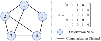
Figure 2: The sensor network topology.

The noisy historical input/output/state trajectories at each node are collected from the linear system (42)–(V-A) with a random initial state. We consider a trajectory length of $N=20$. Moreover, following Theorem 3, $\chi$ is set to $0.1$.

We present the estimation performance of the D-DUIO in Fig. 3, which shows the state estimates obtained over a simulation horizon of $25$ time steps. The plots indicate that all nodes achieve consensus on state estimates with fast convergence rates. Moreover, the state estimation errors shown in Fig. 4 converge to $0$ asymptotically. This demonstrates that inaccurate estimation arising from unknown input and noises can be cancelled by the proposed D-DUIO.

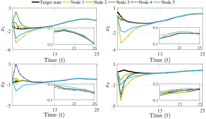
Figure 3: The estimation performance of D-DUIO.

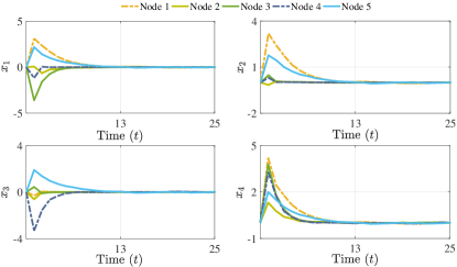
Figure 4: The estimation error of D-DUIO.

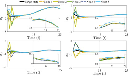
Figure 5: The estimation performance of DUIO [23].

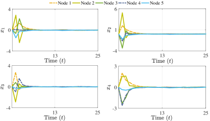
Figure 6: The estimation error of DUIO [23].

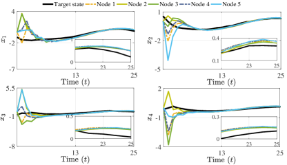
Figure 7: The estimation performance of UI–IKCF [15].

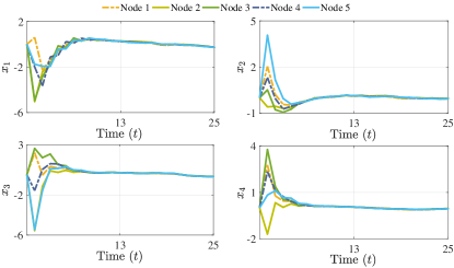
Figure 8: The estimation error of UI–IKCF [15].

V-B Comparison with Model-based DSE Methods

The proposed model-free D-DUIO as well as two model-based DSE methods, namely DUIO [23] and UI-IKCF [15] approaches, are numerically compared in this section.

The special settings for UI-IKCF are given by $S=E[d(k)d^{\top}(k)]=I$, $\Omega_{i}=E[v_{i}(k)v_{i}^{\top}(k)]=I$, and design parameter $\gamma_{i}=2$. For the DUIO, the matrices $E_{i}$, $F_{i}$, $L_{i}$, $H_{i}$, and $P_{i}$ are obtained by solving equations (10) and (15), computed using the CVX toolbox [42]. Parameter $\chi$ is set to $0.5$.

Figures 5–6 and 7–8 show the simulation results of the methods DUIO and UI-IKCF, respectively. Figures 5–6 confirm that the DUIO can guarantee the estimated states of all nodes converge to the target states asymptotically, based on the knowledge of the system model. Figures 7–8 illustrate that UI-IKCF exhibits inferior performance than the other two methods. Due to the measurement noises, the estimation errors of UI-IKCF are only uniformly ultimately bounded rather than converge to $0$. Compared with the DSE methods acting on an exact model, the proposed data-driven method outperforms UI-IKCF and achieves a performance very similar to the one of the DUIO. This indicates the superiority of D-DUIO, since no system model information is required during implementation.

To further discuss the performance of the three methods, the evaluation metric mean-squared error (MSE) is employed from a deterministic viewpoint [15]. We conduct $100$ independent Monte Carlo experiments. For one experiment, the MSE of each node over the time interval $[1,T]$ is defined by ${\rm MSE}_{i}^{1}=(1/T)\sum_{k=1}^{T}[x(k)-\hat{x}_{i}(k)]^{2}$, where $x(k)$ is the true state of the target system, and $\hat{x}_{i}(k)$ is the estimated state of node $i$. The MSE by all estimators becomes ${\rm MSE^{1}}=(1/M)\sum_{i=1}^{M}{\rm MSE}_{i}^{1}$. By $100$ independent experiments, the MSE becomes ${\rm MSE}=(1/100)\sum_{t=1}^{100}{\rm MSE}^{t}$.

Table I presents the MSEs of DUIO, D-DUIO, and UI-IKCF. The proposed D-DUIO method shows a $39.4\%$ reduction in MSE compared to UI-IKCF. The difference between the MSE of D-DUIO and DUIO is $17.8\%$, implying that the DUIO based on the exact model has faster convergence rate than the D-DUIO. Compared to the other two model-based methods, the effectiveness of the proposed D-DUIO is demonstrated.

TABLE I: The MSE of three methods

Method	MSE
Model-based DUIO [23]	0.2427
Data-driven DUIO	0.3433
(D-DUIO) (This paper)
UI-IKCF	0.5622

VI Conclusions

In this paper, we investigated the problem of designing a DUIO for a system, subject to unknown inputs and to process and measurement disturbances, such that the state estimation error asymptotically converges to zero. First, we analyzed the problem using a standard model-based approach, and we provided necessary and sufficient conditions for the problem solvability. Then, we proposed a novel distributed data-driven unknown-input observer (D-DUIO) that estimates the state of the unknown target system. We showed that, under mild assumptions, offline data are representative of any online input/output/state trajectory generated by the system. In addition, any trajectory of the system is compatible with the equations of the proposed D-DUIO, meaning that also the noisy historical data must be compatible with the D-DUIO. Therefore, we used the offline data to design the matrices of the D-DUIO and we provided necessary and sufficient conditions to guarantee that the state estimates across all nodes asymptotically converge to the true state of the system. Finally, we also established the equivalence between the conditions derived in the model-based approach and the ones obtained in the data-driven framework. Simulation results corroborated the effectiveness of the proposed method. Future research directions include extending the results to more complex scenarios such as nonlinear systems and switching network topologies.

References

- [1] R. E. Kalman, “A new approach to linear filtering and prediction problems,” J. Basic Eng., vol. 82, no. 1, pp. 35–45, Mar. 1960.
- [2] D. Luenberger, “An introduction to observers,” IEEE Trans. Autom. Control, vol. 16, no. 6, pp. 596–602, Dec. 1971.
- [3] M. E. Valcher and J. C. Willems, “Observer synthesis in the behavioral approach,” IEEE Trans. Autom. Control, vol. 14, no. 12, pp. 2297–2307, Dec. 1999.
- [4] R. Olfati-Saber, “Distributed Kalman filter with embedded consensus filters,” in Proc. of IEEE Conf. Decis. Control, Seville, Spain, Dec. 12-15, 2005, pp. 8179–8184.
- [5] G. B. Giannakis, V. Kekatos, N. Gatsis, S. J. Kim, H. Zhu, and B. F. Wollenberg, “Monitoring and optimization for power grids: A signal processing perspective,” IEEE Signal Process. Mag., vol. 30, no. 5, pp. 107–128, Aug. 2013.
- [6] A. Ahmad, G. Lawless, and P. Lima, “An online scalable approach to unified multirobot cooperative localization and object tracking,” IEEE Trans. Robot., vol. 33, no. 5, pp. 1184–1199, Oct. 2017.
- [7] G. Battistelli and L. Chisci, “Stability of consensus extended Kalman filter for distributed state estimation,” Automatica, vol. 68, pp. 169–178, June, 2016.
- [8] F. S. Cattivelli and A. H. Sayed, “Diffusion strategies for distributed Kalman filtering and smoothing,” IEEE Trans. Autom. Control, vol. 55, no. 9, pp. 2069–2084, Sept. 2010.
- [9] J. Chen, J. Li, S. Yang, and F. Deng, “Weighted optimization-based distributed Kalman filter for nonlinear target tracking in collaborative sensor networks,” IEEE Trans. Cybern., vol. 47, no. 11, pp. 3892–3905, July, 2016.
- [10] P. Millán, L. Orihuela, C. Vivas, F. Rubio, D. V. Dimarogonas, and K. H. Johansson, “Sensor-network-based robust distributed control and estimation,” Control Eng. Pract., vol. 21, no. 9, pp. 1238–1249, Sept. 2013.
- [11] M. Farina, G. Ferrari-Trecate, and R. Scattolini, “Distributed moving horizon estimation for linear constrained systems,” IEEE Trans. Autom. Control, vol. 55, no. 11, pp. 2462–2475, Mar. 2010.
- [12] R. Olfati-Saber, “Distributed Kalman filtering for sensor networks,” in Proc. of IEEE Conf. Decis. Control, New Orleans, LA, USA, Dec. 12-14, 2007, pp. 5492–5498.
- [13] ——, “Kalman-consensus filter: Optimality, stability, and performance,” in Proc. of IEEE Conf. Decis. Control, Shanghai, China, Dec. 15-18, 2009, pp. 7036–7042.
- [14] A. T. Kamal, J. A. Farrell, and A. K. Roy-Chowdhury, “Information weighted consensus filters and their application in distributed camera networks,” IEEE Trans. Autom. Control, vol. 58, no. 12, pp. 3112–3125, Aug. 2013.
- [15] H. Ji, F. L. Lewis, Z. Hou, and D. Mikulski, “Distributed information-weighted Kalman consensus filter for sensor networks,” Automatica, vol. 77, pp. 18–30, Mar. 2017.
- [16] S. Trimpe and R. D’Andrea, “Event-based state estimation with variance-based triggering,” IEEE Trans. Autom. Control, vol. 59, no. 12, pp. 3266–3281, Aug. 2014.
- [17] Y. S. Shmaliy, F. Lehmann, S. Zhao, and C. K. Ahn, “Comparing robustness of the Kalman, , and UFIR filters,” IEEE Trans. Signal Process., pp. 3447–3458, May, 2018.
- [18] M. E. Valcher, “State observers for discrete-time linear systems with unknown inputs,” IEEE Trans. Autom. Control, vol. 44, no. 2, pp. 397–401, Feb. 1999.
- [19] S. Nazari and B. Shafai, “Distributed unknown input observers for fault detection and isolation,” in Proc. of IEEE Int. Conf. on Control and Autom., Edinburgh, UK, July, 16-19, 2019, pp. 319–324.
- [20] B. L. Nguyen, T. V. Vu, J. M. Guerrero, M. Steurer, K. Schoder, and T. Ngo, “Distributed dynamic state-input estimation for power networks of microgrids and active distribution systems with unknown inputs,” Electric Power Syst. Res., vol. 201, p. 107510, Dec. 2021.
- [21] A. Chakrabarty, S. Sundaram, M. J. Corless, G. T. Buzzard, S. H. Żak, and A. E. Rundell, “Distributed unknown input observers for interconnected nonlinear systems,” in Proc. Amer. Control Conf., Boston, MA, USA, July, 6-8, 2016, pp. 101–106.
- [22] D. Liang, Y. Yang, R. Li, and R. Liu, “Finite-frequency unknown input observer-based distributed fault detection for multi-agent systems,” J. Franklin. Inst., vol. 358, no. 6, pp. 3258–3275, Apr. 2021.
- [23] G. Yang, A. Barboni, H. Rezaee, and T. Parisini, “State estimation using a network of distributed observers with unknown inputs,” Automatica, vol. 146, p. 110631, Dec. 2022.
- [24] Z. Hou and S. Jin, Model-Free Adaptive Control: Theory and Applications. Boca Raton: CRC Press, 2013.
- [25] C. De Persis and P. Tesi, “Formulas for data-driven control: Stabilization, optimality, and robustness,” IEEE Trans. Autom. Control, vol. 65, no. 3, pp. 909–924, Dec. 2020.
- [26] J. C. Willems, P. Rapisarda, I. Markovsky, and B. L. De Moor, “A note on persistency of excitation,” Syst. Control Lett., vol. 54, no. 4, pp. 325–329, Apr. 2005.
- [27] W. Liu, Y. Li, G. Wang, J. Sun, and J. Chen, “Distributed data-driven consensus control of multi-agent systems under switched uncertainties,” Control Theory Technol., vol. 21, pp. 478–487, Sept. 2023.
- [28] W. Liu, J. Sun, G. Wang, F. Bullo, and J. Chen, “Data-driven self-triggered control via trajectory prediction,” IEEE Trans. Autom. Control, vol. 68, no. 11, pp. 6951–6958, Nov. 2023.
- [29] J. Coulson, J. Lygeros, and F. Dörfler, “Data-enabled predictive control: In the shallows of the DeePC,” in Eur. Control Conf., Naples, Italy, June, 25-28, 2019, pp. 307–312.
- [30] J. Berberich, J. Köhler, M. A. Müller, and F. Allgöwer, “Data-driven model predictive control with stability and robustness guarantees,” IEEE Trans. Autom. Control, vol. 66, no. 4, pp. 1702–1717, June, 2020.
- [31] X. Wang, J. Sun, G. Wang, F. Allgöwer, and J. Chen, “Data-driven control of distributed event-triggered network systems,” IEEE/CAA J. Autom. Sinica,, vol. 10, no. 2, p. 351–364, Feb. 2023.
- [32] X. Wang, J. Berberich, J. Sun, G. Wang, F. Allgöwer, and J. Chen, “Model-based and data-driven control of event- and self-triggered discrete-time linear systems,” IEEE Trans. Cybern., vol. 53, no. 9, p. 6066–6079, Sept. 2023.
- [33] Y. Li, X. Wang, J. Sun, G. Wang, and J. Chen, “Data-driven consensus control of fully distributed event-triggered multi-agent systems,” Sci. China Inf. Sci., vol. 66, no. 5, p. 1–15, May, 2023.
- [34] T. M. Wolff, V. G. Lopez, and M. A. Müller, “Data-based moving horizon estimation for linear discrete-time systems,” in Proc. Eur. Control Conf., London, United Kingdom, July, 12-15, 2022, pp. 1778–1783.
- [35] M. S. Turan and G. Ferrari-Trecate, “Data-driven unknown-input observers and state estimation,” IEEE Control Syst. Lett., vol. 6, pp. 1424–1429, Aug. 2021.
- [36] G. Disarò and M. E. Valcher, “On the equivalence of model-based and data-driven approaches to the design of unknown-input observers,” arXiv:2311.00673, Nov. 2023.
- [37] J. Berberich, J. Köhler, M. A. Müller, and F. Allgöwer, “Robust constraint satisfaction in data-driven MPC,” in Proc. of IEEE Conf. on Decis. and Control, Jeju, Korea, Dec. 14-18, 2020, pp. 1260–1267.
- [38] H. Ji, Y. Wei, L. Fan, S. Liu, Z. Hou, and L. Wang, “Data-driven distributed information-weighted consensus filtering in discrete-time sensor networks with switching topologies,” IEEE Trans. Cybern., May, 2022, doi:10.1109/TCYB.2022.3166649.
- [39] M. Bisiacco and M. E. Valcher, “Dead-beat control in the behavioral approach,” IEEE Trans. Autom. Control, vol. 57, no. 9, pp. 2163–2175, Sept. 2012.
- [40] W. Liu, J. Sun, G. Wang, F. Bullo, and J. Chen, “Data-driven resilient predictive control under denial-of-service,” IEEE Trans. Autom. Control, vol. 68, no. 8, pp. 4722–4737, Aug. 2023.
- [41] ——, “Learning robust data-based LQG controllers from noisy data,” arXiv:2305.01417, May, 2023.
- [42] M. Grant and S. Boyd, “CVX: Matlab software for disciplined convex programming, version 2.1,” http://cvxr.com/cvx, Mar. 2014.