Advancing Ante-Hoc Explainable Models through Generative Adversarial Networks

Abstract

This paper presents a novel concept learning framework for enhancing model interpretability and performance in visual classification tasks. Our approach appends an unsupervised explanation generator to the primary classifier network and makes use of adversarial training. During training, the explanation module is optimized to extract visual concepts from the classifier’s latent representations, while the GAN-based module aims to discriminate images generated from concepts, from true images. This joint training scheme enables the model to implicitly align its internally learned concepts with human-interpretable visual properties. Comprehensive experiments demonstrate the robustness of our approach, while producing coherent concept activations. We analyse the learned concepts, showing their semantic concordance with object parts and visual attributes. We also study how perturbations in the adversarial training protocol impact both classification and concept acquisition. In summary, this work presents a significant step towards building inherently interpretable deep vision models with task-aligned concept representations - a key enabler for developing trustworthy AI for real-world perception tasks.

1 Introduction

Deep neural networks (DNNs) have ushered in a revolution across domains like Computer Vision (Simonyan and Zisserman 2015), Natural Language Processing (Brown et al. 2020), Healthcare (Rabbi et al. 2022), and Finance (Heaton, Polson, and Witte 2016). They have made significant strides in handling intricate tasks like image recognition, machine translation, and anomaly detection. However, they come with a challenge - they are essentially black-box systems. The increasing complexity of these models has led to a lack of transparency and interpretability (Lipton 2018; Yeh et al. 2020). This opacity has raised significant concerns within the scientific community, particularly in critical areas like healthcare and criminal justice. In healthcare, for instance, patients would want to know why a disease-diagnosing model provided them with a certain result. Additionally, being able to identify and verify false positives and negatives is essential, as such oversight could have potentially serious consequences.

Explainable models have become instrumental in establishing transparency, a key factor in building trust with users. In recent years, there has been a surge of research in this area, with most works coming under two broad categories: post-hoc and ante-hoc methods.

Post-hoc explainability methods attempt to provide explanations as a separate module on already trained models. Saliency maps (Simonyan, Vedaldi, and Zisserman 2014) are a prime example of this line of work, introducing a method that visually highlights the points on an image that activate neurons, depending on the predicted class by the deep neural network. However, decoupling the explanation method from the explained model makes it a challenge to discern whether the model’s prediction was incorrect or the explanation provided was at fault.

Ante-hoc explainability methods, on the other hand, provide explanations implicitly during model training itself. There have been several ante-hoc works in recent times that make use of concepts (Koh et al. 2020; Doersch, Gupta, and Efros 2015; Zhang, Isola, and Efros 2017). These methods assume that each class can be broken down into a set of concepts, i.e. that concepts can be used to signify the distinctive features or characteristics that make up a particular class. For example, in the case of MNIST (Deng 2012), concepts could include straight lines, types of curves in the digits, or even more specific patterns that may appear in a digit. Self-explaining neural networks (SENN) (Alvarez-Melis and Jaakkola 2018) exemplify such approaches, offering a straightforward means to acquire interpretable concepts by extending a linear predictor. When presented with an input image, the prediction is generated based on a weighted combination of these concepts. (Sarkar et al. 2021) introduce a method to account for varying degrees of concept supervision in a SENN-like framework.

In this paper, we build upon and extend the findings of (Sarkar et al. 2021), showing how introducing an adversarial component into the framework can better guide representation learning. We propose a modified loss, harness the benefits of randomization and use labels as supplementary information for conditioning the reconstruction process.

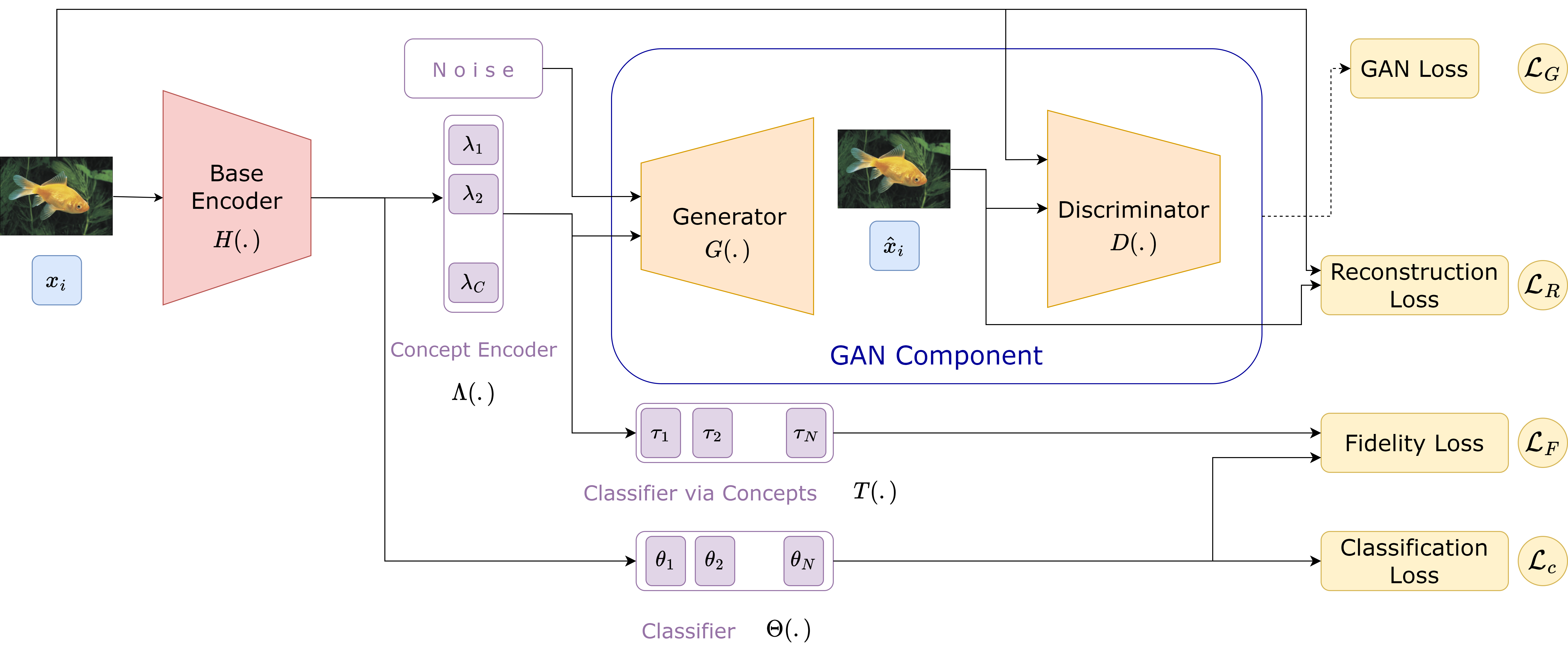
Figure 1: Overview of our Proposed Architecture. N is the number of classes, C is the number of concepts

To summarize, our contributions are as follows:

• We introduce a novel, enhanced architecture that demonstrates improved performance compared to the baselines. The key aspect here lies in the integration of a Generative Adversarial Network (GAN) (Goodfellow et al. 2014) within the architecture.

• We conduct a series of experiments to analyze and compare the impact of different GAN variants, such as a vanilla GAN (Goodfellow et al. 2014) and conditional GAN (cGAN) (Mirza and Osindero 2014), on performance and concept visualization.

• We explore various methods for generating noise to understand how noise sampled from a Gaussian distribution influences concept generation in our framework.

• Our approach capitalizes on the adversarial nature of GANs and noise generation method to produce higher-quality images that facilitate more robust concept encoding.

2 Methodology

2.1 Background

Self Explaining Neural Networks (Alvarez-Melis and Jaakkola 2018): This was one of the first works to propose a robust ante-hoc framework along with metrics to measure interpretability. Starting with a simple linear regression model, which is inherently interpretable - given that the model’s parameters are linearly related, the paper successively generalizes it to more complicated models like neural networks. Their key goals were for concepts to retain image information, to be distinct between classes, and to be understandable to humans. To address these goals, an autoencoder encodes images into concepts optimized using reconstruction and classification losses. One limitation we observe is that the concepts are derived solely from the dataset without leveraging additional information like labels or extra images. Extensions to this attempt to enhance concept explainability through disentanglement and contrastive learning (Sawada and Nakamura 2022). Our work leverages generative models to create more refined concepts that address some of the original limitations.

Ante-Hoc Explainability via Concepts (Sarkar et al. 2021): In this work, an ante-hoc framework, allowing for different levels of supervision, including fully supervised and unsupervised concept learning, was proposed, building upon (Alvarez-Melis and Jaakkola 2018). The framework could be added to any existing backbone model and optimized jointly. The paper primarily introduces the notion of fidelity loss and a way to visualize the concepts learnt by the model. In our work, we assume the basic setup from this paper and make specific modifications to enhance it.

2.2 Proposed Architecture

A typical deep learning classification pipeline has a base encoder function followed by a classifier function. Let $\mathcal{X}$ be the input space and $\mathcal{Y}$ be the label space for our training set $\mathcal{D}=\{x_{i},y_{i}\}_{i=1}^{N}$, sampled iid from some source distribution $\mathcal{P}:\mathcal{X}\times\mathcal{Y}$, where $\mathcal{X}\in\mathrm{R}^{d}$, and $\mathcal{Y}$ is a one-hot encoded vector. The base encoder $H(.)$ extracts representation vectors that are then fed into the classifier $\Theta(.)$. One way of making such a setup interpretable is to provide explanations via concepts. In order to do this, a concept encoder $\Lambda(.)$ is introduced in the pipeline. $\Lambda(.)$ takes in the representations extracted by $H(.)$ and learns a set of concepts $\{\lambda_{1},\lambda_{2},…\lambda_{C}\}$ that are used to explain the classification by passing them through $T(.)$. The concepts are latents that represent the attributes of a class. In our framework, we consider the latents to be scalars representing the degree to which a concept is present in a given image, i.e they are a score. The predictions given by $T$ and $\Theta$ should match, which is enforced through a fidelity loss $\mathcal{L}_{F}$. Further, the concepts learnt are passed through a decoder to reconstruct the input image and as such are enforced to capture image semantics.

Building upon this setup, we have developed a novel architecture incorporating a Generative Adversarial Network (GAN) (Goodfellow et al. 2014) into the framework. GANs consist of two core components: a generator and a discriminator. The primary task of the generator is to fabricate synthetic images or representations that closely mimic a specific dataset or probability distribution. While the discriminator, on the other hand, is responsible for discerning whether an image is authentic or a generated clone. In the above pipeline, we propose sending the concepts to a GAN $(G(.),D(.))$, making use of the adversarial mechanism to retrieve better concepts. $G(.)$ takes in the concepts, supplemented by some noise. The noise introduces a degree of randomness (discussed in Section A.4), which along with the concepts is used to generate an image using deconvolution operations. $\mathcal{L}_{R}$ is needed to enforce that the concepts capture semantics (similar to the role of the decoder in (Sarkar et al. 2021), with noise as an additional input). $D(.)$ takes in an image and outputs whether it is real or fake. So, the loss now becomes:

$$\mathcal{L}= \,\mathcal{L}_{c}+\mathcal{L}_{R}+\mathcal{L}_{F}+\mathcal{L}_{G}$$ (1)

where, $\mathcal{L}_{c}$ is the classification loss, $\mathcal{L}_{R}$ is the reconstruction loss between the input image and the generated image, $\mathcal{L}_{F}$ is the fidelity loss and $\mathcal{L}_{G}$ is the GAN loss.

The discriminator $D(.)$ takes a real image $x_{i}$ and performs a forward pass. The loss and the gradients are then calculated. $D(.)$ also performs a forward pass on the generated image $\hat{x}_{i}$, after which the loss and gradients are calculated. The gradients calculated are passed through $D(.)$ and $G(.)$ as they aren’t detached before being sent to the discriminator. This interconnection ensures that both the generator and discriminator are jointly optimized, working together to produce more convincing fake images while still accurately detecting them. This finishes a single iteration of training the network and the parameters of generator and discriminator are updated for the next round of training.

The overall loss function that we would optimize is:

$$\mathcal{L}= \,\alpha\mathcal{L}_{c}\left(y_{i},\hat{y}_{i}\right)+\beta\mathcal{L}_{R}\left(x_{i},\hat{x}_{i}\right)$$ (2)

$$+\gamma\mathcal{L}_{F}\Bigl{(}\Theta\bigl{(}H(x_{i})\bigr{)},T\bigl{(}\Lambda\bigl{(}H(x_{i})\bigr{)}\bigr{)}\Bigr{)}$$

$$+\delta\mathbb{E}_{x_{i}}\left[\log\,\Bigl{(}D\left(x_{i}\right)\Bigr{)}\right]$$

$$+\delta\mathbb{E}_{n}\left[\log\,\Bigl{(}1-D\bigl{(}G\left(\{\Lambda\left(H(x_{i})\right),n\}\right)\bigr{)}\Bigr{)}\right]$$

In the Eq 2, $\mathcal{L}_{c}$ is cross entropy loss, $\mathcal{L}_{R}$ is the $L_{2}$ loss between the input image and the generated image, $\mathcal{L}_{F}$ is the MSE between the outputs of $\Theta$ and $T$ (Alvarez-Melis and Jaakkola 2018; Sarkar et al. 2021; Lakkaraju, Arsov, and Bastani 2020), and the remaining two terms are the GAN loss $\mathcal{L}_{G}$. $\alpha,\beta,\gamma,\delta$ are arbitrary terms for linear combination that have been introduced from an implementation and empirical perspective. $n$ is the noise that has been sampled using methods in Section A.4 of the appendix.

The rationale behind using GANs stems from the desire to provide a substantially broader spectrum for the concepts to be learnt from. In a GAN framework, the input to the generator is typically sampled from a normal distribution. However, in our methodology, we adopt an approach that combines inputs from both a normal distribution and the encoding. This choice effectively enlarges the feature space available to the generator. Although this increases model complexity, it helps capture richer concepts that can be validated from the figures. Consequently, it empowers the generator to adeptly reconstruct images from the encoding. This, we posit, ultimately leads to an enhancement in the encoder’s proficiency in generating more informative encodings.

3 Experiments and Results

We carry out a set of experiments to compare and demonstrate the performance of our framework and show several variations of models. The baseline is the method from (Sarkar et al. 2021), which builds upon and outperforms SENN (Alvarez-Melis and Jaakkola 2018) on CIFAR-10 and CIFAR-100. We provide the dataset details in section A.4 of the appendix. We reimplement their code and hyperparameters to ensure model/hardware differences don’t impact results. For SENN, we use the results reported by (Sarkar et al. 2021) (They do not report aux. acc. on CIFAR100). Our evaluation criteria are $\Theta$ classification accuracy (top 1% accuracy) and $T$ classification accuracy, referred to as accuracy and auxiliary accuracy. Given the necessity of maintaining faithful and explainable concepts, while providing accurate image classification, we give a higher importance to accuracy. We briefly describe our evaluation criteria below:

Accuracy (top 1% accuracy): This metric corresponds to the classification accuracy for the input images with respect to the ground truth labels.

Auxiliary Accuracy (Alvarez-Melis and Jaakkola 2018): This metric corresponds to the classification accuracy based on the output from $T(.)$ and its proficiency in predicting the class labels.

3.1 Comparative Analysis

Our objective with the experiments was to first identify optimal models within each GAN category and various VGG network variations, and subsequently conduct a comparative study with the baselines. To assess the robustness of the models, we employ a training process repeated five times with distinct random seeds. The resulting accuracies are averaged to yield a final assessment. We chose a batch size of 32 for processing images, following (Sarkar et al. 2021), to keep the results consistent and comparable. Additionally, the noise length is set to 10, mirroring the size of concepts in the CIFAR-10 dataset, in order to ensure that the noise makes a substantial contribution to the learned concepts.

Label conditioning impact: We conduct experiments on Vanilla GAN (Goodfellow et al. 2014) and cGAN (Mirza and Osindero 2014) to assess the impact of label conditioning on our framework. Vanilla GAN generates images from random noise without specific constraints, lacking precise control over image generation. While cGAN leverages labels as an additional input parameter to control the generation of the image. For example, if the network is trained on pictures of different animals, one cannot specify which animal the generator should create. Some slight modifications are made to the network to ensure its compatibility with both Vanilla GAN and cGAN, ensuring that our framework is adaptable to both types of GANs. We conduct experiments using different noise generation techniques on different variants of Vanilla GAN and cGAN, with the best methods being chosen for comparison with the baselines. This analysis is provided in section A.4 of the appendix.

Model	VGG Model	Method	Acc.	Aux. Acc.
Baselines	NA	NA	64.46	44.65
SENN	NA	NA	36.57	NA
Vanilla GAN (B=32, S=10)	11	DAN	65.49	45.05
Vanilla GAN (B=32, S=10)	19	DAN	60.71	44.52
cGAN (B=32, S=10)	11	DAN	65.37	45.36
cGAN (B=32, S=10)	19	DAN	64.42	44.92

Table 1: Accuracy (in %) and Auxiliary Accuracy (in %) for comparison with the baseline and SENN on CIFAR100. cGAN = Conditional GAN, B = Batch Size, S = size of noise. We see that our method classifies better.

Model	VGG Model	Method	Acc.	Aux. Acc.
Baseline	NA	NA	91.68	90.86
SENN	NA	NA	84.50	84.50
Vanilla GAN (B=32, S=10)	8	ICN	91.57	89.63
Vanilla GAN (B=32, S=10)	11	ICN	91.66	90.04
cGAN(B=32, S=10)	8	PCN	91.60	89.94
cGAN(B=32, S=10)	11	DAN	91.58	89.90
cGAN(B=32, S=5)	19	DAN	91.82	90.23

Table 2: Accuracy (in %) and Auxiliary Accuracy (in %) for comparison with the baseline and SENN on CIFAR10. cGAN = Conditional GAN, B = Batch Size, S = size of noise. We see that our method classifies better.

Tables 1 and 2 show the CIFAR10 and CIFAR100 comparisons across architectures of different configurations with the baselines. The best model overall was cGAN with VGG19 and a noise size of 5 giving a 91.82% accuracy on CIFAR10. For CIFAR100, Vanilla GAN with VGG11-DAN achieved the highest accuracy of 65.49%. Although the configuration with the best auxiliary accuracy was cGAN with VGG11-DAN at 45.36%.

Concept Visualization: We visualize the top 5 images where a particular concept $\lambda_{i}$ had the highest score as compared to the other concepts. So the images visualize the captured concepts, or activate a particular concept. We also show that concepts are captured across classes. Using this method, we show the concepts captured by our best model using CIFAR100 in Fig 2 and by our best model using CIFAR10 in Fig 3. Additional concept visualizations for other model and noise configurations are provided in Section A.5 of the appendix.

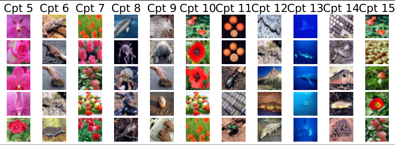
Figure 2: Top 5 images for CIFAR100 that activate the learnt concepts (10 concepts from a subset of 100) using cGAN (VGG 19) DAN (B=32, S=10). Eg: Cpt 5 corresponds to color pink, Cpt 13 corresponds to object in ocean.

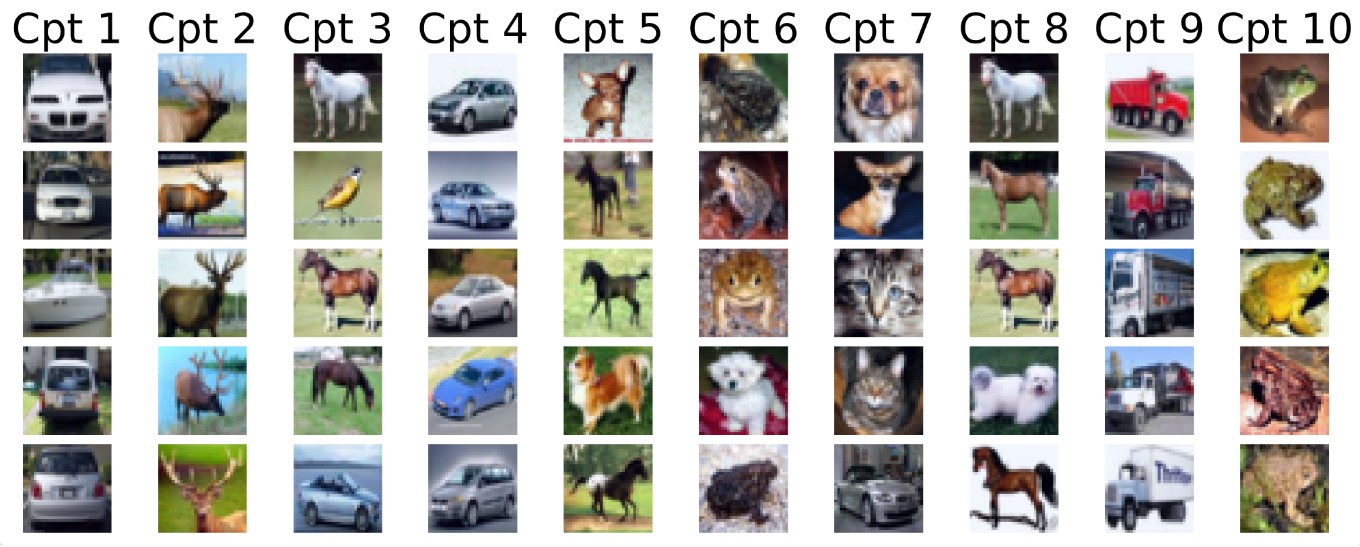
Figure 3: Top 5 images for CIFAR10 that activate the learnt concepts using cGAN (VGG 11) DAN (B=32, S=10). Eg: Cpt 2 captures antlers, Cpt 1 captures the color white - here we see that activated images are from different classes (ship, car).

3.2 Observations

The preceding sections discussed how various VGG models can influence the performance of our framework. Our observations underline that GAN-based conditioning, cGAN, introduces notable improvements. A general trend observed indicates that VGG model depth correlates with improved performance, particularly in terms of accuracy. We also see that a correlation between dataset scale and auxiliary accuracy, from the fact that our method consistently gives better auxiliary accuracy compared to the baselines on CIFAR100.

Another significant observation is that the increasing complexity of the model due to the GAN integration and noise sampling methodologies (as detailed in Section A.4 of appendix); increase training time by 1.4 times that of (Sarkar et al. 2021). Despite this, the training efficiency remains considerably superior to that of SENN.

4 Conclusion and Future Work

In conclusion, this work presents a method for incorporating a Generative Adversarial Network (GAN) into an ante-hoc explainability framework. The design replaces a conventional decoder network with a GAN and fine-tunes the framework. The exploration of noise sampling methods, specifically the implementation of DAN, demonstrate superior performance, proving the effectiveness of a GAN in aiding the process of encoding concepts. We have observed results that signify an improved overall accuracy and auxiliary accuracy, highlighting the potential of our architecture for robust image classification and effective concept learning.

Although, we have made some improvements on enhancing the explainability of deep neural networks without losing out on classification performance, the work presented is a small step towards a much more robust and human interpretable model. In the future, we plan on exploring the possibilities of more advanced and complex architectures that could involve using a much deeper classification models such as ResNet, EfficientNet, Mask RCNN. We also plan on making use of the capabilities of some state-of-the-art architectures such as Vision Transformers in conjunction with our framework. Another empirical observation we made is that different noise methods work well for different configurations. We plan on further analysis along this direction.

Appendix A Appendix

A.1 Acknowledgements

We would like to thank the authors of (Sarkar et al. 2021) for their guidance and insighful discussions. We would also like to thank the anonymous reviewers for their valuable feedback.

A.2 Related Work

Post-Hoc Methods: In addition to Saliency Maps (Simonyan, Vedaldi, and Zisserman 2014) and Grad-CAM (Selvaraju et al. 2017), other influential post-hoc techniques include LIME (Ribeiro, Singh, and Guestrin 2016) and DeepLift (Shrikumar, Greenside, and Kundaje 2017). LIME provides model-agnostic local explanations by approximating any classifier with an interpretable linear model. DeepLift decomposes the predictions of a Deep Neural Network by backpropagating contribution scores to the inputs. Most of these methods are gradient-based, with the problem of the root cause of errors being difficult to diagnose.

Concept-based Models: (Koh et al. 2020) propose concept bottleneck models with a concept layer to improve interpretability and enable test-time human intervention. These models are trained on both task labels and user-specified concepts via a two-step process where inputs predict concepts and concepts predict labels. This interpretable structure allows for interventions, where experts can correct wrong predictions by modifying concept values, enabling model interaction. However, intervention effectiveness depends on the training approach, highlighting the need to study factors beyond just accuracy. While subsequent works expanded these ideas (Chauhan et al. 2023; Zarlenga et al. 2022; Yuksekgonul, Wang, and Zou 2022), there has been some criticism as to whether these models truly learn as intended (Margeloiu et al. 2021).

Prototype-based Learning: (Li et al. 2018) introduce an approach for interpreting deep neural networks by integrating an autoencoder with a prototype layer during training. The model classifies inputs based on their proximity to encoded examples in the prototype layer, facilitating an intuitive case-based reasoning mechanism. The jointly optimized prototypes, guided by various loss terms, connect the network’s decisions with explanations, visible through visualization of class-representative prototypes. While achieving competitive accuracy compared to CNN baselines, the method offers integrated explanations without post-hoc techniques. Several extensions to prototype-based methods have been proposed, like (Chen et al. 2019; Donnelly, Barnett, and Chen 2022)

Other methods: Several prior studies have developed methods focusing on both high accuracy and explainability. Some methods take the approach of making use of auto-encoders that could enable the reconstruction of images such as (Zhang, Isola, and Efros 2017). There human-in-the-loop works related to involving human feedback and developing concepts that both align with human’s intuition of concept such as (Lage and Doshi-Velez 2020). Several derivatives of prototype-based models have proven to be quite impressive at visualizing representations and explanations (Biehl, Hammer, and Villmann 2016).

A.3 Implementation Details

All our experiments were conducted on NVIDIA GeForce GTX 1080 Ti. The generator architecture comprises multiple deconvolution layers, generating images using learned concepts and noise, and incorporating labels in the case of cGAN. The discriminator architecture has a VGG network backbone with few additional layers to re-purpose it into a binary classifier. We have tested with different VGG (Simonyan and Zisserman 2015) architectures such as VGG 8, VGG 11 and VGG 19.

A.4 Datasets and Comparison Methods

Datasets: For our experiments, we choose the CIFAR-10 and CIFAR-100 (Krizhevsky 2009) benchmarks to facilitate comparisons with prior work. CIFAR-10 consists of 60,000 32x32 coloured images from 10 classes, with 6,000 images per class. The dataset split of 50,000/10,000 train/test images providing sufficient data for training deep networks while maintaining a separate test set for unbiased evaluation. CIFAR-100 is slightly more challenging, containing the same number of images but partitioning them into 100 classes, each with 600 images. This increased class variability and lower samples per class simulate real-world fine-grained classification challenges more closely. Compared to CIFAR-10, CIFAR-100 tests a model’s ability to discriminate between subtle inter-class differences.

We chose CIFAR-10 and CIFAR-100 as their moderate sizes allowed us to conduct extensive experiments in reasonable time to thoroughly test different architectures and design decisions, as compared to huge datasets such as ImageNet (Deng et al. 2009). Both the datasets contain complex and diverse real life objects in various backgrounds.

Noise Methods: This study introduces a framework with an emphasis on the integration of noise into the network, typically drawn from a Normal distribution $\mathcal{N}(0,1)$. The impact of various noise sampling techniques on GAN training has been thoroughly studied. Given the batch size $B$ of images as 32, concepts of size 10, and a designated noise size $S$ of 5, the shape of the concepts and the noise would be 32x10x1 ($B\times C\times 1$) and 32x5x1 ($B\times S\times 1$), respectively. Once the noise is added, the final shape of the concepts would be 32x15x1 ($B\times(C+S)\times 1$). Different noise generation strategies are explored. The noise sampled helped us in determining the effects of different noise perturbations on our model.

Method 1: Direct Align Noise (DAN): The noise is directly aligned with batch size and noise length. Consequently, the sampled noise follows the shape ($B\times S\times 1$) where the entire ($B\times S\times 1$) matrix is sampled from $\mathcal{N}(0,1)$ and together represents a Gaussian.

Method 2: Iterative Concat Noise (ICN): The noise is sampled multiple times to achieve the desired dimension. Initially, noise is sampled as $B\times 1\times 1$ and then concatenated $S$ times. Each row of size $B\times 1\times 1$ is sampled from a Gaussian.

Method 3: Progressive Concat Noise (PCN): The noise is sampled multiple times, but it begins with an even smaller dimension. Noise is initially sampled as $1\times S\times 1$ and then concatenated $B$ times. Each column of size $1\times S\times 1$ is sampled from a Gaussian.

We show that introducing noise improves model adaptability, enhancing image quality and overall model efficiency. One point to note is that the ICN and PCN vectors, when concatenated may not represent a Gaussian. Our framework can be extended to incorporate other noise methods as well.

Model	VGG Model	DAN		ICN		PCN
		Accuracy	Aux. Accuracy	Accuracy	Aux. Accuracy	Accuracy	Aux. Accuracy
cGAN (B=32, S=10)	11	65.37	45.36	65.15	41.69	65.21	45.44
cGAN (B=32, S=10)	19	64.42	44.92	62.42	44.87	64.00	44.56
Vanilla GAN (B=32, S=10)	11	65.49	45.05	65.13	46.16	65.47	45.80
Vanilla GAN (B=32, S=10)	19	60.71	44.52	58.09	43.78	60.02	46.19

Table 3: Accuracy (in %) and Auxiliary Accuracy in (%) for comparing our models on CIFAR100. cGAN = Conditional GAN, B = Batch Size, S = size of Noise. Aux. Accuracy = Auxiliary Accuracy. We see that different noise methods work well on different models. We are choosing the best noise method.

Model	VGG Model	DAN		ICN		PCN
		Accuracy	Aux. Accuracy	Accuracy	Aux. Accuracy	Accuracy	Aux. Accuracy
Vanilla GAN (B=32, S=10)	8	91.53	90.00	91.57	89.63	91.41	89.57
Vanilla GAN (B=32, S=10)	11	91.38	89.63	90.80	89.37	91.66	90.94
cGAN (B=32, S=10)	8	91.55	90.15	91.44	90.13	91.60	89.94
cGAN (B=32, S=10)	11	91.58	89.90	91.34	89.96	91.28	89.82
cGAN (B=32, S=5)	11	91.36	89.74	91.44	89.77	91.47	89.68
cGAN (B=32, S=10)	19	91.52	90.09	91.76	90.08	91.45	89.99
cGAN (B=32, S=5)	19	91.82	90.23	91.15	89.62	91.44	89.60

Table 4: Accuracy (in %) and Auxiliary Accuracy in (%) for comparing our models on CIFAR10. cGAN = Conditional GAN, B = Batch Size, S = size of Noise. Aux. Accuracy = Auxiliary Accuracy. We see that different noise methods work well on different models.

A.5 Additional Results

This section displays additional concept visualization results that could not be included in the main paper. These results are based on CIFAR10 as well as CIFAR100 for both Vanilla GAN and Conditional GAN.

We also perform comparative analysis on different noise methods (discussed in Section A.4) on our framework with different VGG models and both Vanilla GAN and Conditional GAN.

Vanilla GAN: As shown in Table 4, in the case of CIFAR10, for VGG 8, we observe that ICN gives the best accuracy of 91.57%. While in the case of VGG 11, PCN gives better results, with an accuracy of 91.66%. As shown in Table 3, on CIFAR100, for VGG 11 we observe that DAN has the best accuracy of 65.49%. DAN also gives the best accuracy of 60.71% for VGG 19.

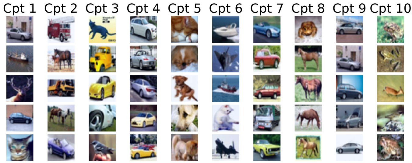
Figure 4: Top 5 images for CIFAR10 that activate the learnt concepts using cGAN (VGG 19) DAN (B=32, S=5). Eg: Cpt 9 captures a concept corresponding to the grey color, Cpt 10 corresponds to frog skin.

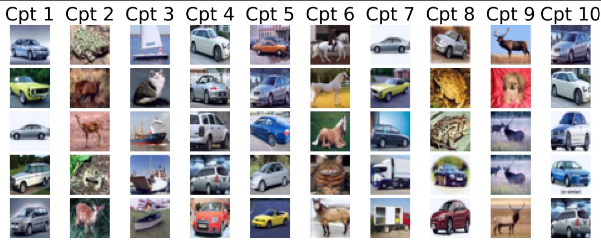
Figure 5: Top 5 images for CIFAR10 that activate the learnt concepts using Vanilla GAN (VGG 8) ICN (B=32, S=10). Eg: Cpt 9 corresponds to antlers, Cpt 6 corresponds to shape of legs.

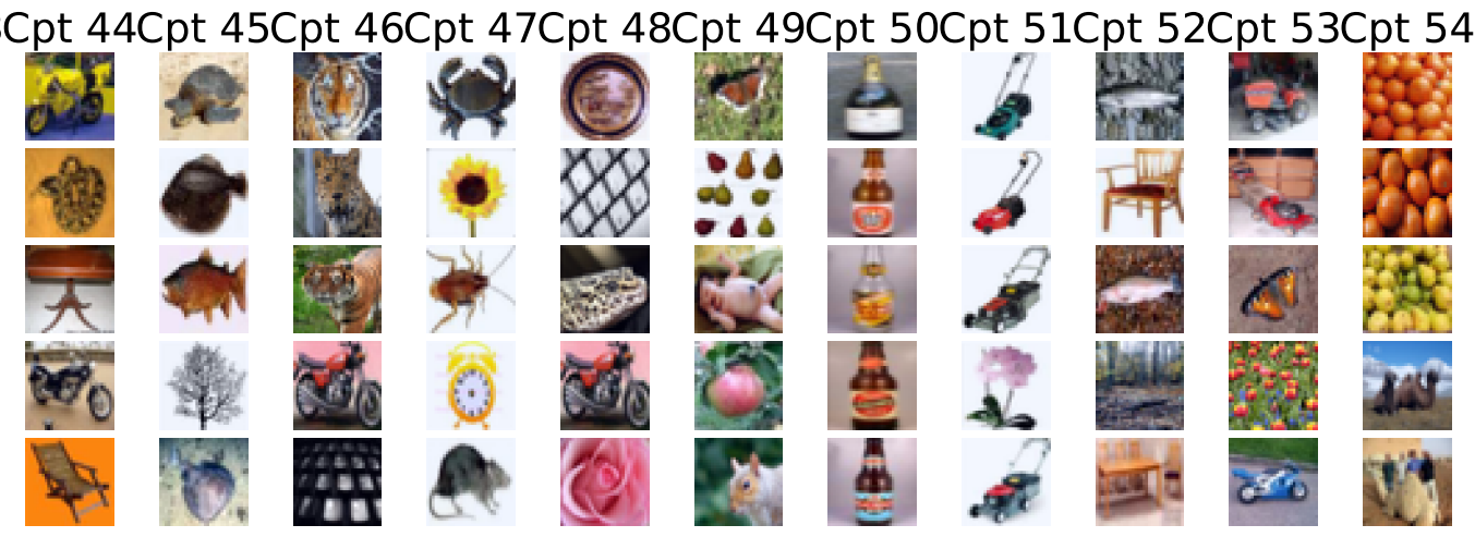
Figure 6: Top 5 images for CIFAR100 that activate the learnt concepts (10 concepts from a subset of 100) using cGAN (VGG 11) PCN (B=32, S=10). Eg: Cpt 50 corresponds to shape of a bottle, and Cpt 51 corresponds to a lawn-mower.

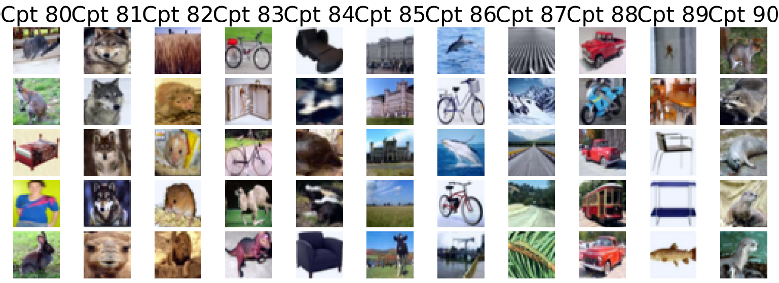
Figure 7: Top 5 images for CIFAR100 that activate the learnt concepts (10 concepts from a subset of 100) using Vanilla GAN (VGG 11) DAN (B=32, S=10). Eg: Cpt 81 corresponds to face of a wolf, Cpt 88 corresponds to wheels.

cGAN: Here, in addition to a noise size of 10, we also experiment with a noise size of 5 to examine its effect on the framework. As shown in Table 4, for CIFAR10, using VGG 8, PCN gives the best accuracy of 91.60%. In the case of VGG 11, for a noise size of 10, we get better results using DAN - with an accuracy of 91.58%; whereas for a noise size of 5, we get better results using PCN - with an accuracy of 91.47%. Finally, in the case of VGG 19, DAN gives the best results when using a noise size of 5. As shown in Table 3, for CIFAR100, we consistently observe that DAN gives the best results. In the case of VGG 11, using DAN we get the best accuracy of 65.37%. With VGG 19, using DAN we get the best accuracy of 64.42%.

References

- Alvarez-Melis and Jaakkola (2018) Alvarez-Melis, D.; and Jaakkola, T. S. 2018. Towards Robust Interpretability with Self-Explaining Neural Networks. In Bengio, S.; Wallach, H. M.; Larochelle, H.; Grauman, K.; Cesa-Bianchi, N.; and Garnett, R., eds., Advances in Neural Information Processing, NeurIPS 2018, December 3-8, 2018, Montréal, Canada, 7786–7795.
- Biehl, Hammer, and Villmann (2016) Biehl, M.; Hammer, B.; and Villmann, T. 2016. Prototype-based Models for the Supervised Learning of Classification Schemes. Proceedings of the International Astronomical Union, 12(S325): 129–138.
- Brown et al. (2020) Brown, T.; Mann, B.; Ryder, N.; Subbiah, M.; Kaplan, J. D.; Dhariwal, P.; Neelakantan, A.; Shyam, P.; Sastry, G.; Askell, A.; Agarwal, S.; Herbert-Voss, A.; Krueger, G.; Henighan, T.; Child, R.; Ramesh, A.; Ziegler, D.; Wu, J.; Winter, C.; Hesse, C.; Chen, M.; Sigler, E.; Litwin, M.; Gray, S.; Chess, B.; Clark, J.; Berner, C.; McCandlish, S.; Radford, A.; Sutskever, I.; and Amodei, D. 2020. Language Models are Few-Shot Learners. In Larochelle, H.; Ranzato, M.; Hadsell, R.; Balcan, M.; and Lin, H., eds., Advances in Neural Information Processing Systems, NeurIPS 2020, volume 33, 1877–1901. Curran Associates, Inc.
- Chauhan et al. (2023) Chauhan, K.; Tiwari, R.; Freyberg, J.; Shenoy, P.; and Dvijotham, K. 2023. Interactive concept bottleneck models. In Proceedings of the AAAI Conference on Artificial Intelligence, volume 37, 5948–5955.
- Chen et al. (2019) Chen, C.; Li, O.; Tao, C.; Barnett, A. J.; Su, J.; and Rudin, C. 2019. This Looks like That: Deep Learning for Interpretable Image Recognition. Red Hook, NY, USA: Curran Associates Inc.
- Deng et al. (2009) Deng, J.; Dong, W.; Socher, R.; Li, L.-J.; Li, K.; and Fei-Fei, L. 2009. ImageNet: A large-scale hierarchical image database. In 2009 IEEE Conference on Computer Vision and Pattern Recognition, 248–255.
- Deng (2012) Deng, L. 2012. The MNIST Database of Handwritten Digit Images for Machine Learning Research [Best of the Web]. IEEE Signal Processing Magazine, 29(6): 141–142.
- Doersch, Gupta, and Efros (2015) Doersch, C.; Gupta, A.; and Efros, A. A. 2015. Unsupervised Visual Representation Learning by Context Prediction. In Proceedings of the IEEE International Conference on Computer Vision (ICCV).
- Donnelly, Barnett, and Chen (2022) Donnelly, J.; Barnett, A. J.; and Chen, C. 2022. Deformable ProtoPNet: An Interpretable Image Classifier Using Deformable Prototypes. In Proceedings of the IEEE/CVF Conference on Computer Vision and Pattern Recognition (CVPR), 10265–10275.
- Goodfellow et al. (2014) Goodfellow, I.; Pouget-Abadie, J.; Mirza, M.; Xu, B.; Warde-Farley, D.; Ozair, S.; Courville, A.; and Bengio, Y. 2014. Generative adversarial nets. In Advances in neural information processing systems, NeurIPS 2014, 2672–2680.
- Heaton, Polson, and Witte (2016) Heaton, J. B.; Polson, N. G.; and Witte, J. H. 2016. Deep Learning in Finance. CoRR, abs/1602.06561.
- Koh et al. (2020) Koh, P. W.; Nguyen, T.; Tang, Y. S.; Mussmann, S.; Pierson, E.; Kim, B.; and Liang, P. 2020. Concept Bottleneck Models. In III, H. D.; and Singh, A., eds., Proceedings of the 37th International Conference on Machine Learning, volume 119 of Proceedings of Machine Learning Research, 5338–5348. PMLR.
- Krizhevsky (2009) Krizhevsky, A. 2009. Learning Multiple Layers of Features from Tiny Images.
- Lage and Doshi-Velez (2020) Lage, I.; and Doshi-Velez, F. 2020. Learning Interpretable Concept-Based Models with Human Feedback. presented at the International Conference on Machine Learning: Workshop on Human Interpretability in Machine Learnin, 1: 1–11.
- Lakkaraju, Arsov, and Bastani (2020) Lakkaraju, H.; Arsov, N.; and Bastani, O. 2020. Robust and Stable Black Box Explanations. In III, H. D.; and Singh, A., eds., Proceedings of the 37th International Conference on Machine Learning, volume 119 of Proceedings of Machine Learning Research, 5628–5638. PMLR.
- Li et al. (2018) Li, O.; Liu, H.; Chen, C.; and Rudin, C. 2018. Deep Learning for Case-Based Reasoning through Prototypes: A Neural Network That Explains Its Predictions. In Proceedings of the Thirty-Second AAAI Conference on Artificial Intelligence and Thirtieth Innovative Applications of Artificial Intelligence Conference and Eighth AAAI Symposium on Educational Advances in Artificial Intelligence, AAAI’18/IAAI’18/EAAI’18. AAAI Press. ISBN 978-1-57735-800-8.
- Lipton (2018) Lipton, Z. C. 2018. The Mythos of Model Interpretability: In Machine Learning, the Concept of Interpretability is Both Important and Slippery. Queue, 16(3): 31–57.
- Margeloiu et al. (2021) Margeloiu, A.; Ashman, M.; Bhatt, U.; Chen, Y.; Jamnik, M.; and Weller, A. 2021. Do Concept Bottleneck Models Learn as Intended? arXiv:2105.04289.
- Mirza and Osindero (2014) Mirza, M.; and Osindero, S. 2014. Conditional Generative Adversarial Nets. CoRR, abs/1411.1784.
- Rabbi et al. (2022) Rabbi, F.; Dabbagh, S. R.; Angin, P.; Yetisen, A. K.; and Tasoglu, S. 2022. Deep Learning-Enabled Technologies for Bioimage Analysis. Micromachines, 13(2).
- Ribeiro, Singh, and Guestrin (2016) Ribeiro, M. T.; Singh, S.; and Guestrin, C. 2016. ”Why Should I Trust You?”: Explaining the Predictions of Any Classifier. In Proceedings of the 22nd ACM SIGKDD International Conference on Knowledge Discovery and Data Mining, KDD ’16, 1135–1144. New York, NY, USA: Association for Computing Machinery. ISBN 9781450342322.
- Sarkar et al. (2021) Sarkar, A.; Vijaykeerthy, D.; Sarkar, A.; and Balasubramanian, V. N. 2021. A Framework for Learning Ante-hoc Explainable Models via Concepts. 2022 IEEE/CVF Conference on Computer Vision and Pattern Recognition (CVPR), 10276–10285.
- Sawada and Nakamura (2022) Sawada, Y.; and Nakamura, K. 2022. C-SENN: Contrastive Self-Explaining Neural Network. arXiv:2206.09575.
- Selvaraju et al. (2017) Selvaraju, R. R.; Cogswell, M.; Das, A.; Vedantam, R.; Parikh, D.; and Batra, D. 2017. Grad-CAM: Visual Explanations from Deep Networks via Gradient-Based Localization. In 2017 IEEE International Conference on Computer Vision (ICCV), 618–626.
- Shrikumar, Greenside, and Kundaje (2017) Shrikumar, A.; Greenside, P.; and Kundaje, A. 2017. Learning Important Features through Propagating Activation Differences. In Proceedings of the 34th International Conference on Machine Learning - Volume 70, ICML’17, 3145–3153. JMLR.org.
- Simonyan, Vedaldi, and Zisserman (2014) Simonyan, K.; Vedaldi, A.; and Zisserman, A. 2014. Deep Inside Convolutional Networks: Visualising Image Classification Models and Saliency Maps. In Bengio, Y.; and LeCun, Y., eds., 2nd International Conference on Learning Representations, ICLR 2014, Banff, AB, Canada, April 14-16, 2014, Workshop Track Proceedings.
- Simonyan and Zisserman (2015) Simonyan, K.; and Zisserman, A. 2015. Very Deep Convolutional Networks for Large-Scale Image Recognition. In Bengio, Y.; and LeCun, Y., eds., 3rd International Conference on Learning Representations, ICLR 2015, San Diego, CA, USA, May 7-9, 2015, Conference Track Proceedings.
- Yeh et al. (2020) Yeh, C.-K.; Kim, B.; Arik, S.; Li, C.-L.; Pfister, T.; and Ravikumar, P. 2020. On Completeness-aware Concept-Based Explanations in Deep Neural Networks. In Larochelle, H.; Ranzato, M.; Hadsell, R.; Balcan, M.; and Lin, H., eds., Advances in Neural Information Processing Systems, volume 33, 20554–20565. Curran Associates, Inc.
- Yuksekgonul, Wang, and Zou (2022) Yuksekgonul, M.; Wang, M.; and Zou, J. 2022. Post-hoc Concept Bottleneck Models. In ICLR 2022 Workshop on PAIR^2Struct: Privacy, Accountability, Interpretability, Robustness, Reasoning on Structured Data.
- Zarlenga et al. (2022) Zarlenga, M. E.; Barbiero, P.; Ciravegna, G.; Marra, G.; Giannini, F.; Diligenti, M.; Shams, Z.; Precioso, F.; Melacci, S.; Weller, A.; Lio, P.; and Jamnik, M. 2022. Concept Embedding Models. In Oh, A. H.; Agarwal, A.; Belgrave, D.; and Cho, K., eds., Advances in Neural Information Processing Systems.
- Zhang, Isola, and Efros (2017) Zhang, R.; Isola, P.; and Efros, A. A. 2017. Split-Brain Autoencoders: Unsupervised Learning by Cross-Channel Prediction. In Proceedings of the IEEE Conference on Computer Vision and Pattern Recognition (CVPR).