Coordinate descent methods beyond smoothness and separability

Abstract

This paper deals with convex nonsmooth optimization problems. We introduce a general smooth approximation framework for the original function and apply random (accelerated) coordinate descent methods for minimizing the corresponding smooth approximations. Our framework covers the most important classes of smoothing techniques from the literature. Based on this general framework for the smooth approximation and using coordinate descent type methods we derive convergence rates in function values for the original objective. Moreover, if the original function satisfies a growth condition, then we prove that the smooth approximations also inherits this condition and consequently the convergence rates are improved in this case. We also present a relative randomized coordinate descent algorithm for solving nonseparable minimization problems with the objective function relative smooth along coordinates w.r.t. a (possibly nonseparable) differentiable function. For this algorithm we also derive convergence rates in the convex case and under the growth condition for the objective.

1 Introduction

In this paper we study (accelerated) random (block) coordinate descent methods for solving nonsmooth convex optimization problems of the form:

$$F^{*}=\min_{x\in\mathbb{R}^{n}}F(x),\vspace{-0.4cm}$$ (1)

where $F:\mathbb{R}^{n}\to\bar{\mathbb{R}}$ is a general proper closed convex function (possibly nonseparable). First order methods for nonsmooth optimization, e.g. subgradient type methods, have convergence rates of order $\mathcal{O}(1/\epsilon^{2})$, where $\epsilon$ is the desired accuracy for the approximate solution. In order to improve convergence, smooth approximations of the original function can be considered and gradient type methods [1] can be used for solving these smooth approximations. Some examples of smoothing techniques are Moreau envelope [2], Forward-Backward envelope [3, 4], Douglas-Rachford envelope [3, 5], Nesterov’s smoothing [6] and Gaussian smoothing [7]. General properties for these smoothing techniques can be found in [3, 6, 7, 5, 2, 4, 8, 9]. Moreover, in e.g., [6, 7, 8, 9] gradient type methods are considered for solving the smooth approximation. However, in large-scale problems the computation of the full gradient of the smooth approximation can be prohibitive. In this case one can use coordinate descent algorithms [10, 11, 12, 13] for solving the smooth approximation, as it was done e.g., in [14, 15, 12]. On other hand, if the original function is still nonsmooth, but relative smooth w.r.t. a differentiable function, coordinate descent type methods still converge (sub)linearly [16]. Some examples of convex relative smooth functions were given in [16]. Relative coordinate descent algorithms were also considered in [17, 18, 19]. However, in all these papers the original function is relative smooth along coordinates with respect to a separable function.

Previous work: In [6] the following problem is considered

$$F(x)=f(x)+\max_{u\in Q}\left\{\langle Ax,u\rangle-{\phi}(u)\right\},\vspace{-0.1cm}$$ (2)

with the gradient of $f$ assumed Lipschitz and a smooth approximation was proposed for this problem, which we call in this paper Nesterov’s smoothing. Moreover, [6] also presents an accelerated gradient descent method for solving the smooth approximation for which sublinear rate is obtained in the convex case. In the context of coordinate descent algorithms, [12] presents an accelerated coordinate descent algorithm for solving the Nesterov’s smooth approximation. Paper [15] considers the problem (2) with $f$ being separable, i.e., $f(x)=\sum_{i=1}^{N}f_{i}(x_{i})$, and considers the Nesterov’s smoothing for the second term of the objective. Finally, a coordinate descent algorithm is used for solving the smooth approximation and rates of order $\mathcal{O}\left(\frac{1}{\epsilon^{2}}\log\left(\frac{1}{\epsilon}\right)\right)$ are derived in the convex case and improved to $\mathcal{O}\left(\frac{1}{\epsilon}\log\left(\frac{1}{\epsilon}\right)\right)$, when the smooth approximation is strongly convex. Moreover, in [14] an objective function of the form

$$F(x)=\frac{1}{2}x^{T}Ax+b^{T}x+\psi(x)\vspace{-0.1cm}$$ (3)

is considered, with $b\in\mathbb{R}^{n}$, $A\in\mathbb{R}^{n\times n}$ is a symmetric positive semidefinite matrix and $\psi$ is a proper closed convex function (possibly nonsmooth and nonseparable) which is proximal easy. Then, the Forward-Backward envelope is employed as a smooth approximation for the objective and a modified accelerated coordinate descent algorithm is used for solving this smooth approximation (in each iteration it is necessary to compute two proximal operators). Rate of order $\mathcal{O}\left(\frac{1}{\epsilon^{3/2}}\right)$ is obtained in function values at some point $\Pi_{\text{dom}\psi}(x)$, where $\Pi_{\text{dom}\psi}(\cdot)$ is the projection onto the domain of $\psi$, provided that $\psi$ is Lipschitz in any bounded subset. Finally, when the function is relative smooth along coordinates in [18] a relative randomized coordinate descent is proposed and sublinear rates are obtained in the convex case and linear rates for an objective that is relative strong with respect to a separable function.

Contributions. In this paper we first introduce a general smoothing framework for the convex objective function $F$ in problem (1) and we use random (accelerated) coordinate descent methods from the literature to solve the smooth approximation. We also present a relative randomized coordinate descent algorithm for minimizing convex objective functions that are relative smooth along coordinates w.r.t. a (possibly nonseparable) differentiable function. More precisely, our main contributions are:

(i) We introduce a novel smoothing framework for general nonsmooth and nonseparable convex objective functions (Assumption 1), which covers in particular the most important smooth approximations from the literature (Moreau envelope, Forward-Backward envelope, Douglas-Rachford envelope and Nesterov’s smoothing). In the Moreau envelope, we assume that $F$ is a proper closed convex function and proximally easy. In the Forward-Backward and Douglas-Rachford envelopes our results are valid when $F$ has the form (3). In the Douglas-Rachford envelope, matrix $\left(I_{n}+\gamma A\right)^{-1}$ must be computed easily, where $\gamma>0$ is the parameter of the smoothing and $I_{n}$ is the identity matrix. Finally, for Nesterov’s smoothing our framework covers the case when $f$ has coordinate-wise Lipschitz gradient in the problem (2). Then, we consider random (accelerated) coordinate descent algorithms for solving this smooth approximation. Under this general framework we derive sublinear convergence rates in function values for the original problem (1).

(ii) Moreover, the rates are improved (to even linear) if the original objective function satisfies a $q$-growth condition (Assumption 3). We prove that Moreau envelope, Forward-Backward envelope and Nesterov’s smoothing inherits such a $q$-growth. Table 1 summarizes the main convergence results from this paper for each smoothing technique, where $\bar{\kappa}$ is the constant in Assumption 3.

(iii) We also consider nonsmooth objective functions (possibly nonseparable), but relative smooth along coordinates with respect to a given function (possibly also nonseparable). For this problem a relative randomized coordinate descent algorithm is introduced, for which we derive sublinear rate when the objective $F$ is convex. Moreover, if the function $F$ satisfies a $q$-growth condition, we prove that the algorithm converges linearly with high probability.

The major difference between our result corresponding to the Forward-Backward envelope and the result in [14] is that a rate of order $\mathcal{O}(1/k^{1.5})$ is obtained in [14] in function values at the point $\Pi_{\text{dom}\psi}(x_{k})$, where $x_{k}$ is the iterate of the accelerated algorithm in [14], while we derive an improved rate of order $\mathcal{O}(1/k^{2})$ in function values at the point $\text{prox}_{\gamma\psi}\left(x_{k}-\gamma\nabla f(x_{k})\right)$, where $x_{k}$ is the iterate of our Algorithm 2. Another major difference is that the modified accelerated coordinate descent algorithm considered in [14] requires computation of two proximal operators of $\psi$ per iteration, while in the algorithm considered in this paper only one proximal operator of $\psi$ is computed at each iteration. Moreover, in [14] an extra assumption that $\psi$ is Lipschitz in any bounded subset is required, while we do not need this assumption to obtain our convergence rates.

	ME	FB	DR	NS	Result
Coordinate Descent Method
Convex	$1/\epsilon$	$1/\epsilon$	$1/\epsilon$	$1/\epsilon^{2}$	Thm 4
$q$-growth	$\ln\left(1/\epsilon\right)$	$\ln\left(1/\epsilon\right)$	-	$(1/\epsilon)\ln\left(1/\epsilon\right)$	Thm 8
Accelerated Coordinate Descent Method
Convex	$1/\sqrt{\epsilon}$	$1/\sqrt{\epsilon}$	$1/\sqrt{\epsilon}$	$1/\epsilon$	Thm 6
Restart Accelerated Coordinate Descent Method knowing a lower bound $\bar{\kappa}$
$q$-growth	$\ln\left(1/\epsilon\right)$	$\ln\left(1/\epsilon\right)$	-	$(1/\sqrt{\epsilon})\ln\left(1/\epsilon\right)$	Cor 2
Restart Accelerated Coordinate Descent Method not knowing $\bar{\kappa}$
$q$-growth	$\ln\left(\frac{1}{\epsilon}\right)\log_{2}\left(\ln\left(\frac{1}{\epsilon}\right)\right)$		-	$\left(\frac{1}{\sqrt{\epsilon}}\right)\ln\left(\frac{1}{\epsilon}\right)\log_{2}\left(\ln\left(\frac{1}{\epsilon}\right)\right)$	Thm 9

Table 1: Convergence rates derived in this paper for Moreau envelope (ME), Forward-Backward (FB) envelope, Douglas-Rachford (DR) envelope and Nesterov’s smoothing (NS) in the convex and $q$-growth cases.

Content. The paper is organized as follows. In Section 1.1 we present some definitions and preliminary results. We introduce our general smoothing framework in Section 2. In Section 3 we analyze the $q$-growth condition. Then, in Section 4, we consider random (accelerated) coordinate descent algorithms and derive convergence rates in function values of the original objective in the convex and $q$-growth cases. In Section 5, we present a relative smooth coordinate descent algorithm and derive convergence in the convex and $q$-growth cases. Finally, in Section 6 we provide detailed numerical simulations.

1.1 Preliminaries

In this section we present some notations, definitions and some preliminary results. Let $U\in\mathbb{R}^{n\times n}$ be a column permutation of the $n\times n$ identity matrix and further let $U=[U_{1},...,U_{N}]$ be a decomposition of $U$ into $N$ submatrices, with $U_{i}\in\mathbb{R}^{n\times n_{i}}$, where $\sum_{i=0}^{N}n_{i}=n$. Any vector $x\in\mathbb{R}^{n}$ can be written uniquely as $x=\sum_{i=0}^{N}U_{i}x^{(i)}$, where $x^{(i)}=U_{i}^{T}x\in\mathbb{R}^{n_{i}}$. For spaces $R^{n_{i}}$, let us fix some norms $\|\cdot\|_{(i)}$, $i=1,\cdots,N$. Moreover, $\|x\|^{2}=\sum_{i=1}^{N}\|x^{(i)}\|^{2}$ is defined as the Euclidean norm and $\|\cdot\|_{\ell_{p}}$ is the $\ell_{p}$ norm, for $p\neq 2$. We consider $\delta_{B}$ the indicator function of the set $B$ and $e_{i}$ is the $i$-th component vector of the canonical basis. We denote with $X^{*}$ the set of minimizers of problem (1) and with $\bar{x}=[x]_{X^{*}}$, the projection of $x$ onto $X^{*}$ (all the letters with bar above denote the projection of a point onto $X^{*}$). For a given function $F$ and $y\in\text{dom}F$ its level set is defined as

$$\mathcal{L}_{F}(y)=\{x\in\text{dom}F:\;F(x)\leq F(y)\}.$$

Next, we present the definition of convexity along coordinates.

Definition 1.

For any fixed $x\in\mathbb{R}^{n}$ and $i=1,\cdots,N$ denote $\phi^{x}_{i}:\mathbb{R}^{n_{i}}\to\mathbb{R}$ as:

$$\phi^{x}_{i}(d)=\psi(x+U_{i}d).$$ (4)

We say that $\psi:\mathbb{R}^{n}\to\mathbb{R}$ is (strictly) convex along coordinates if the partial functions $\phi^{x}_{i}:\mathbb{R}^{n_{i}}\to\mathbb{R}$ are (strictly) convex for all $x\in\mathbb{R}^{n}$ and $i=1,\cdots,N$.

Let us define the notion of block coordinate-wise Lipschitz gradient [13].

Definition 2.

Given a closed convex set $X\subseteq\mathbb{R}^{n}$ and a differentiable function $f:\mathbb{R}^{n}\to\mathbb{R}$. The gradient of $f$ is block coordinate-wise Lipschitz continuous on $X$, with constants $L_{i}>0$, if for all $x,x+U_{i}h\in X$ and $i=1,\cdots,N$, the following inequality holds

$$\|U_{i}^{T}(\nabla f(x+U_{i}h)-\nabla f(x))\|_{(i)}\leq L_{i}\|h\|_{(i)}.$$ (5)

If (5) holds, then we have the following relation [13]:

$$|f(x+U_{i}h)-f(x)-\langle U_{i}^{T}\nabla f(x),h\rangle|\leq\frac{L_{i}}{2}\|h\|^{2}_{(i)}.$$ (6)

When $N=1$ in the inequality above, we say the function $f$ has Lipschitz gradient. Next result was proved for the case $N=1$, see for example [1, Thm 2.1.5]. We adapt this result for the (block) coordinate case.

Lemma 1.

Consider $f:\mathbb{R}^{n}\to\mathbb{R}$ a function and $X\subseteq\mathbb{R}^{n}$ a closed convex set. Assume that $f$ is convex along coordinates and the following inequality holds for all $x,x+U_{i}h\in X$ and $i=1,\cdots,N$

$$f(x+U_{i}h)-f(x)-\langle U_{i}^{T}\nabla f(x),h\rangle\leq\dfrac{L_{i}}{2}\|h\|_{(i)}^{2}.$$ (7)

Then, we have:

$$f(x+U_{i}h)-\langle U_{i}^{T}\nabla f(x+U_{i}h),h\rangle+\dfrac{1}{2L_{i}}\|U_{i}^{T}(\nabla f(x+U_{i}h)-\nabla f(x))\|^{2}_{(i)}\leq f(x),$$

and

$$\|U_{i}^{T}(\nabla f(x+U_{i}h)-\nabla f(x))\|_{(i)}\leq L_{i}\|h\|_{(i)}.$$

Proof.

See appendix for a proof. ∎

2 Smooth approximations for convex problems

In this section we introduce a general smoothing framework for convex functions. Our framework covers the most important smoothing techniques from literature: Moreau, Forward-Backward, Douglas-Rachford envelope and Nesterov’s smoothing.

Assumption 1.

Consider $F_{\gamma}(x)$, a smooth approximation for the function $F$ (with parameter $\gamma>0$). Assume that:

• A.1 Consider $F_{\gamma}^{*}=\min F_{\gamma}(x)$. We have that $F_{\gamma}^{*}\leq F^{*}$.

• A.2 There exist operators $\mathcal{B}$ and $\mathcal{C}$ and some constant $D\geq 0$ such that

  $$F(\mathcal{B}(x))-\gamma D\leq F_{\gamma}(x)\leq F(\mathcal{C}(x)),\quad\forall x\in\text{dom}F.\vspace{-0.2cm}$$

• A.3 The gradient of $F_{\gamma}$ is block coordinate-wise Lipschitz continuous on $\mathbb{R}^{n}$, with constants $L_{i}(F_{\gamma})>0$, see Definition 2.

• A.4 $F_{\gamma}(x)$ is convex.

Next, we give some examples of smooth approximations that satisfy Assumption 1. The reader may find others examples of smoothing techniques that fit our framework.

2.1 Moreau envelope

As a first example of a smoothing technique we have the Moreau Envelope [2]. The Moreau envelope of a function $F$ with $\gamma>0$ is defined as

$$F_{\gamma}(x):=\min_{u\in\mathbb{R}^{n}}\left\{F(u)+\dfrac{1}{2\gamma}\|u-x\|^{2}\right\},$$ (8)

while the minimizer of the problem above, called proximal mapping, is

$$\text{prox}_{\gamma F}(x):=\arg\min_{u\in\mathbb{R}^{n}}\left\{F(u)+\dfrac{1}{2\gamma}\|u-x\|^{2}\right\}.$$ (9)

Below, we show that the Moreau Envelope satisfies Assumption 1:

A.1 It is well-known that [2]:

$$F^{*}=\min_{x\in\mathbb{R}^{n}}F(x)=\min_{x\in\mathbb{R}^{n}}F_{\gamma}(x)=F^{*}_{\gamma}\quad\text{and}\quad\arg\min_{x\in\mathbb{R}^{n}}F(x)=\arg\min_{x\in\mathbb{R}^{n}}F_{\gamma}(x).$$ (10)

A.2 Consider $\hat{u}=\text{prox}_{\gamma F}(x)$. A direct implication from the definition of $F_{\gamma}$ is that $F(\hat{u})\leq F_{\gamma}(x)\leq F(x)$, for all $\gamma>0$. Hence $\mathcal{B}(x)=\text{prox}_{\gamma F}(x)$, $\mathcal{C}$ is the identity operator and $D=0$.

A.3 If $F$ is a proper closed convex function, then $F_{\gamma}$ is differentiable and its gradient [2]

$$\nabla F_{\gamma}(x)=\gamma^{-1}\left(x-\text{prox}_{\gamma F}(x)\right)$$ (11)

is $\gamma^{-1}$-Lipschitz continuous. Moreover, note that the coordinate-wise Lipschitz constant of $\nabla F_{\gamma}$ is also $L_{i}(F_{\gamma})=\gamma^{-1}$. In fact,

$$\|U_{i}^{T}(\nabla F_{\gamma}(x+U_{i}h)-\nabla F_{\gamma}(x))\|_{(i)}\leq\|\nabla F_{\gamma}(x+U_{i}h)-\nabla F_{\gamma}(x)\|\leq\gamma^{-1}\|h\|_{(i)}.$$

A.4 If $F$ is convex, then $F_{\gamma}$ is also convex (see for example [2]).

2.2 Forward-Backward envelope

Consider the problem (1) defined as the following composite problem

$$F^{*}=\min_{x\in\mathbb{R}^{n}}F(x):=f(x)+\psi(x),$$ (12)

where $\psi$ is a proper closed convex function. Moreover, $\psi$ is proximal easy and $f$ has Lipschitz gradient with constant $L>0$. The Forward-Backward envelope of the pair $(f,\psi)$ with a smooth parameter $\gamma>0$ is the function [3, 4]:

$$F_{\gamma}(x)=f(x)-\dfrac{\gamma}{2}\|\nabla f(x)\|^{2}+\psi^{\gamma}(x-\gamma\nabla f(x)),$$ (13)

where $\psi^{\gamma}$ is the Moreau envelope of the function $\psi$ defined in (8). Note that the Forward-Backward envelope can also be defined as

$$F_{\gamma}(x)=\min_{u\in\mathbb{R}^{n}}f(x)+\langle\nabla f(x),u-x\rangle+\dfrac{1}{2\gamma}\|u-x\|^{2}+\psi(u).\vspace{-0.2cm}$$ (14)

Now, we summarize the results obtained in [3, 4] that fits in our framework. If $f$ is twice differentiable and has Lipschitz gradient, and $\psi$ is a proper closed convex function, then $F_{\gamma}$ is continuously differentiable with

$$\nabla F_{\gamma}(x)=\gamma^{-1}\left(I-\gamma\nabla^{2}f(x)\right)\left[x-\text{prox}_{\gamma\psi}(x-\gamma\nabla f(x))\right].$$ (15)

Moreover, Forward-Backward envelope satisfies Assumption 1 when $f$ is quadratic:

A.1 For all $\gamma L\in\left(0,1\right]$, we have

$$\arg\min_{x\in\mathbb{R}^{n}}F(x)\subset\arg\min_{x\in\mathbb{R}^{n}}F_{\gamma}(x)\quad\text{and}\quad F^{*}=\min_{x\in\mathbb{R}^{n}}F(x)=\min_{x\in\mathbb{R}^{n}}F_{\gamma}(x)=F^{*}_{\gamma}.$$ (16)

Moreover, if $\gamma L\in\left(0,1\right)$, we have

$$\arg\min_{x\in\mathbb{R}^{n}}F(x)=\arg\min_{x\in\mathbb{R}^{n}}F_{\gamma}(x).$$ (17)

A.2 Consider $\hat{u}=\text{prox}_{\gamma\psi}\left(x-\gamma\nabla f(x)\right)$, recall that $F(\hat{u})\leq F_{\gamma}(x)$ for $\gamma L\in\left(0,1\right]$. Moreover, from the definition of $F_{\gamma}$, we have $F_{\gamma}(x)\leq F(x)$, for all $\gamma>0$. Hence, $\mathcal{B}(x)=\text{prox}_{\gamma\psi}\left(x-\gamma\nabla f(x)\right)$, $\mathcal{C}$ is the identity operator and $D=0$.

A.3 Consider

$$F(x)=f(x)+\psi(x)=\frac{1}{2}x^{T}Ax+b^{T}x+\psi(x),$$ (18)

for $A\in\mathbb{R}^{n\times n}$ a symmetric positive semidefinite matrix and $b\in\mathbb{R}^{n}$ and $\psi$ is a proper closed convex function. Then, (15) becomes

$$\nabla F_{\gamma}(x)=\gamma^{-1}\left(I-\gamma A\right)\left[x-\text{prox}_{\gamma\psi}(x-\gamma\nabla f(x))\right].$$ (19)

If $\gamma L\in\left(0,1\right)$, then the gradient (19) is Lipschitz continuous with constant $\gamma^{-1}(1-\gamma\lambda_{\min}(A))$, where $\lambda_{\min}(A)$ is the smallest eigenvalue of A. Moreover, for $\gamma L\in\left(0,1\right)$, using Proposition 4.3 in [3] and Lemma 1, we get that the $i$th coordinate-wise Lipschitz constant of $\nabla F_{\gamma}$ in (19) is

$$L_{i}(F_{\gamma})=\dfrac{\|U_{i}^{T}\left(I_{n}-\gamma A\right)U_{i}\|}{\gamma}=\dfrac{\|I_{n_{i}}-\gamma A_{ii}\|}{\gamma}.$$

Note that the gradient, $\nabla F_{\gamma}$, from (19) is in fact Lipschitz and block coordinate-wise Lipschitz for all $\gamma>0$. However, the Lipschitz and coordinate-wise Lipschitz constants take larger values when $\gamma L\geq 1$ than when $\gamma L<1$. In fact, a more general result holds, i.e., the gradient, $\nabla F_{\gamma}$, given in (15) is Lipschitz (coordinate-wise Lipschitz) on a set $X\subset\mathbb{R}^{n}$ when $f$ is convex, the hessian of $f$ is Lipschitz (coordinate-wise Lipschitz) and there exists a constant $R>0$ such that $\|x-\text{prox}_{\gamma\psi}(x-\gamma\nabla f(x))\|\leq R\quad\forall x\in X$. However, in our analysis we consider $\gamma L\in\left(0,1\right)$ and $f$ quadratic, since under these conditions convexity is also preserved, see the next statement.

A.4 When $\gamma L\in\left(0,1\right)$ and $F$ is defined as in (18), we have $F_{\gamma}$ also convex, see [3, Proposition 4.4].

2.3 Douglas-Rachford envelope

Let us present the results obtained in [3, 5] that are relevant in this paper. Consider the problem (12) where $\psi$ is a proper closed convex function and $f$ has Lipschtz gradient with constant $L>0$. The Douglas-Rachford envelope for the problem (12) is defined as:

$$F_{\gamma}(x)=f^{\gamma}(x)-\gamma\|\nabla f^{\gamma}(x)\|^{2}+\psi^{\gamma}(x-2\gamma\nabla f^{\gamma}(x)),$$ (20)

where $f^{\gamma},\psi^{\gamma}$ are the Moreau Envelopes of the functions $f$ and $\psi$, defined in (8). The Douglas-Rachford envelope can also be expressed as

$$F_{\gamma}(x)=\min_{u\in\mathbb{R}^{n}}f\left(P_{\gamma}(x)\right)+\langle\nabla f\left(P_{\gamma}(x)\right),u-P_{\gamma}(x)\rangle+\dfrac{1}{2\gamma}\|u-P_{\gamma}(x)\|^{2}+\psi(u),\vspace{-0.2cm}$$

with $P_{\gamma}(x)\!=\!\text{prox}_{\gamma f}(x)$. Moreover, Douglas-Rachford envelope satisfies Assumption 1 when f is quadratic:

A.1 If $\gamma L\in\left(0,1\right)$ we have:

$$F^{*}=\min_{x\in\mathbb{R}^{n}}F(x)=\min_{x\in\mathbb{R}^{n}}F_{\gamma}(x)=F_{\gamma}^{*}\quad\text{and}\quad\arg\min_{x\in\mathbb{R}^{n}}F(x)=\text{prox}_{\gamma f}\left(\arg\min_{x\in\mathbb{R}^{n}}F_{\gamma}(x)\right).\vspace{-0.2cm}$$

A.2 Consider $\hat{u}=\text{prox}_{\gamma f}(x)$ and $\hat{v}=\text{prox}_{\gamma\psi}\left(2\hat{u}-x\right)$, if $\gamma L\in\left(0,1\right)$ we have $F(\hat{v})\leq F_{\gamma}(x)$. Moreover, $F_{\gamma}(x)\leq F(\hat{u})$, for all $\gamma>0$. Hence $\mathcal{B}(x)=\text{prox}_{\gamma\psi}\left(2\text{prox}_{\gamma f}(x)-x\right)$, $\mathcal{C}(x)=\text{prox}_{\gamma f}(x)$ and $D=0$.

A.3 Consider $F$ defined as in (18). If $\gamma L\in\left(0,1\right)$ we have $\nabla F_{\gamma}$ is Lipschitz continuous:

$$\nabla F_{\gamma}(x)=\dfrac{1}{\gamma}\left(\dfrac{2}{\gamma}\left(\gamma^{-1}I_{n}+A\right)^{-1}-I_{n}\right)G(x),\vspace{-0.2cm}$$

with

$$G(x) =\left(\gamma^{-1}I_{n}+A\right)^{-1}(\gamma^{-1}x-b)-\text{prox}_{\gamma\psi}\left(2\left(\gamma^{-1}I_{n}+A\right)^{-1}(\gamma^{-1}x-b)-x\right).$$

Matrix $\left(I_{n}+\gamma A\right)^{-1}$ can be computed easily e.g., when $A$ is block diagonal. For (18), using Proposition 4.5 in [3] and Lemma 1, we get that the coordinate-wise Lipschitz constant of $\nabla F_{\gamma}$ is $L_{i}(F_{\gamma})=\dfrac{\|U_{i}^{T}\left(P+P^{2}\right)U_{i}\|}{\gamma}$, with $P=2\left(I_{n}+\gamma A\right)^{-1}-I_{n}$.

A.4 When $\gamma L\in\left(0,1\right)$ and $F$ is defined as (18), we have $F_{\gamma}$ also convex, see [3, Proposition 4.6].

2.4 Nesterov’s smoothing

Consider the function

$$F(x)=f(x)+\max_{u\in Q}\left\{\langle Ax,u\rangle-{\phi}(u)\right\},\vspace{-0.2cm}$$ (21)

where $Q\subset\mathbb{R}^{m}$ is a closed convex bounded subset, ${\phi}$ a continuous convex function on Q, and $f$ a convex function having a coordinate-wise Lipschitz gradient, with constants $L_{i}(f)>0$, for $i=1,\cdots,N$. Examples of function that satisfies (21) can be found in [6]. Let us recall the main properties of Nesterov’s smoothing [6, 12]:

$$F_{\gamma}(x)={\color[rgb]{0,0,0}f(x)}+\max_{u\in Q}\left\{\langle Ax,u\rangle-{\phi}(u)-\gamma d(u)\right\},\vspace{-0.2cm}$$ (22)

where $d$ is strongly convex function on $Q$ w.r.t. some norm $\|\cdot\|_{W}$ with parameter $\sigma>0$ and $d(u)\geq 0$ for all $u\in Q$. Then, Nesterov’s smoothing satisfies Assumption 1:

A.1 Defining $\bar{D}=\max_{u}d(u)$, we have that:

$$F_{\gamma}(x)\leq F(x)\leq F_{\gamma}(x)+\gamma\bar{D},\quad\forall x\in\mathbb{R}^{n},\vspace{-0.2cm}$$ (23)

Hence $F_{\gamma}^{*}\leq F^{*}$.

A.2 From (23), we have $D=\bar{D}$. Moreover, $\mathcal{B}$ and $\mathcal{C}$ are the identity operators.

A.3 The gradient of $F_{\gamma}$ is

$$\nabla F_{\gamma}(x)=\nabla f(x)+A^{T}u_{\gamma}(x),\vspace{-0.2cm}$$ (24)

where $u_{\gamma}(x)$ is the unique solution of the optimization problem in (22). Moreover, the gradient of $F_{\gamma}$ is coordinate-wise Lipschitz with constant

$$L_{i}(F_{\gamma})=L_{i}(f)+\dfrac{1}{\gamma}\left(\|Ae_{i}\|^{*}_{U}\right)^{2},\;\text{where}\;\|Ae_{i}\|_{U}^{*}=\max_{u}\{\langle Ae_{i},u\rangle:\|u\|_{U}\leq 1\}.\vspace{-0.2cm}$$ (25)

A.4 Note that $F_{\gamma}$ is a maximum of linear functions in $x$, hence it is convex.

Based on the previous examples, we can see that our framework is general and covers a wide range of smoothing techniques.

3 Functional $q$-growth

Strong convexity type conditions, such as $q$-growth property, allow to derive linear rates for first order methods, see [20]. In this section we prove that smooth approximations of objective functions satisfying some $q$-growth condition inherits such a property. Recall that $X^{*}$ is the set of minimizers of problem (1) and $\bar{x}=[x]_{X^{*}}$ is the projection of $x$ onto $X^{*}$. In this section we consider the following additional assumption on $F$.

Assumption 2.

Consider $X\subseteq\text{dom}F$. We assume that the function $F$ satisfies a functional $q$-growth on $X$, i.e., there exists a constant $\kappa>0$ and $q\in[1,2]$ such that:

$$F(x)-F^{*}\geq\dfrac{\kappa}{q}\|x-\bar{x}\|^{q}\quad\forall x\in X.\vspace{-0.2cm}$$

Below, we prove that Moreau envelope, Forward-Backward envelope and Nesterov’s smoothing satisfy also a $q$-growth like condition. Let us introduce some notations that will be used in the sequel. We define $\displaystyle L_{\max}=\max_{i=1:N}L_{i}(F_{\gamma})$. We consider the following norms, for $\alpha\in\mathbb{R}$:

$$\|x\|^{2}_{\alpha}=\sum_{i=1}^{N}(L_{i}(F_{\gamma}))^{\alpha}\|x^{(i)}\|^{2}_{(i)}.$$

3.1 Moreau and Forward-Backward envelopes

Theorem 1.

Let Assumption 2 hold for a given function $F$ and $X=\mathcal{L}_{F}(x_{0})$. For $q\in[1,2)$ assume additionally that the level set of the smooth approximation $F_{\gamma}$ satisfies:

$$\|x-\bar{x}\|\leq R\quad\forall x\in\mathcal{L}_{F_{\gamma}}(x_{0})\quad{\color[rgb]{0,0,0}\text{and some}\quad R>0.}\vspace{-0.2cm}$$

If $F$ is a proper closed convex function and $F_{\gamma}$ is the Moreau envelope, then it satisfies the following inequality:

$$F_{\gamma}(x)-F^{*}_{\gamma}\geq\dfrac{\hat{\kappa}}{2}\|x-\bar{x}\|^{2}_{1}\quad\forall x\in\mathcal{L}_{F_{\gamma}}(x_{0}),\vspace{-0.2cm}$$ (26)

with

$$\hat{\kappa}=\left\{\begin{array}[]{ll}\dfrac{\kappa\gamma}{(\gamma\kappa+1)}\;\text{ if }q=2\\ \dfrac{\kappa^{2}\gamma^{2}}{(\kappa\gamma+R^{2-q})^{2}}\;\text{ if }q\in[1,2).\end{array}\right.$$ (27)

If $F=f+\psi$, such that $f$ has Lipschitz gradient with constant $L>0$, $\psi$ is a proper closed convex function and $F_{\gamma}$ is the Forward-Backward envelope with $\gamma L\in(0,1)$, then it satisfies (26) with

$$\hat{\kappa}=\left\{\begin{array}[]{ll}\dfrac{\kappa(1-\gamma L)}{(\gamma\kappa+1-\gamma L)L_{\max}(F_{\gamma})}\;\text{ if }q=2\\ \dfrac{\kappa^{2}\gamma(1-\gamma L)}{(\kappa\gamma+R^{2-q}(1-\gamma L))^{2}L_{\max}(F_{\gamma})}\;\text{ if }q\in[1,2).\end{array}\right.$$ (28)

Proof.

Let us first prove the case of Moreau envelope. Consider $x\in\mathcal{L}_{F_{\gamma}}(x_{0})$ and $z=\text{prox}_{\gamma F}(x)$. Note that $z\in\mathcal{L}_{F}(x_{0})$. Since $F$ is a proper closed convex function and satisfies the $q$-growth condition, then we have:

$$F_{\gamma}(x)-F^{*}_{\gamma}=F(z)+\dfrac{1}{2\gamma}\|z-x\|^{2}-F^{*} \geq\dfrac{\kappa}{q}\|z-\bar{z}\|^{q}+\dfrac{1}{2\gamma}\|z-x\|^{2}$$

$$\geq\min_{u\in\mathbb{R}^{n}}\dfrac{\kappa}{q}\|u-{\color[rgb]{0,0,0}\bar{z}}\|^{q}+\dfrac{1}{2\gamma}\|u-x\|^{2}.\vspace{-0.2cm}$$

For $q=2$, from the optimality condition (considering $u$ the optimal point of the previous problem), we get:

$$\kappa(u-{\color[rgb]{0,0,0}\bar{z}})+\dfrac{1}{\gamma}(u-x)=0\iff u=\dfrac{1}{\kappa\gamma+1}x+\dfrac{\gamma\kappa}{\gamma\kappa+1}{\color[rgb]{0,0,0}\bar{z}},\vspace{-0.2cm}$$

and we obtain

$$\min_{u\in\mathbb{R}^{n}}\dfrac{\kappa}{2}\|u-{\color[rgb]{0,0,0}\bar{z}}\|^{2}+\dfrac{1}{2\gamma}\|u-x\|^{2}=\dfrac{\kappa}{2(\gamma\kappa+1)}\|x-{\color[rgb]{0,0,0}\bar{z}}\|^{2}\geq\dfrac{\kappa}{2(\gamma\kappa+1)L_{\max}(F_{\gamma})}\|x-\bar{x}\|^{2}_{1}.\vspace{-0.2cm}$$

Since $L_{i}(F_{\gamma})=\gamma^{-1}$, for $i=1,\cdots,N$, in the Moreau envelope, then $F_{\gamma}$ is 2-growth w.r.t. the norm $\|\cdot\|_{1}$, with constant $\hat{\kappa}=\dfrac{\kappa\gamma}{(\gamma\kappa+1)}$.

For $q\in[1,2)$, considering $u={\color[rgb]{0,0,0}\bar{z}}$, we get

$$\min_{u\in\mathbb{R}^{n}}\dfrac{\kappa}{q}\|u-{\color[rgb]{0,0,0}\bar{z}}\|^{q}+\dfrac{1}{2\gamma}\|u-x\|^{2}=\dfrac{1}{2\gamma}\|{\color[rgb]{0,0,0}\bar{z}}-x\|^{2}\geq\dfrac{1}{2\gamma}\|\bar{x}-x\|^{2}=\dfrac{1}{2}\|\bar{x}-x\|^{2}_{1}.\vspace{-0.2cm}$$

On other hand, considering $u\neq{\color[rgb]{0,0,0}\bar{z}}$, from the optimality conditions there exists $u$:

$$\kappa\|u-{\color[rgb]{0,0,0}\bar{z}}\|^{q-2}\left(u-{\color[rgb]{0,0,0}\bar{z}}\right)+\dfrac{1}{\gamma}\left(u-x\right)=0.\vspace{-0.2cm}$$

Define $\alpha=\kappa\|u-{\color[rgb]{0,0,0}\bar{z}}\|^{q-2}$ and $\beta=\dfrac{1}{\gamma}$, then from equality above we get

$$\alpha(u-{\color[rgb]{0,0,0}\bar{z}})+\beta(u-x)=0\Leftrightarrow(\alpha+\beta)u=\alpha{\color[rgb]{0,0,0}\bar{z}}+\beta x\;\;\Leftrightarrow\;\;u=\dfrac{\alpha}{\alpha+\beta}{\color[rgb]{0,0,0}\bar{z}}+\dfrac{\beta}{\alpha+\beta}x.\vspace{-0.2cm}$$

This implies that

$$\min_{u\in\mathbb{R}^{n}}\dfrac{\kappa}{q}\|u-{\color[rgb]{0,0,0}\bar{z}}\|^{q}+\dfrac{1}{2\gamma}\|u-x\|^{2}$$

$$=\dfrac{\kappa}{q}\left\|\dfrac{\alpha}{\alpha+\beta}{\color[rgb]{0,0,0}\bar{z}}+\dfrac{\beta}{\alpha+\beta}x-{\color[rgb]{0,0,0}\bar{z}}\right\|^{q}+\dfrac{1}{2\gamma}\left\|\dfrac{\alpha}{\alpha+\beta}{\color[rgb]{0,0,0}\bar{z}}+\dfrac{\beta}{\alpha+\beta}x-x\right\|^{2}$$

$$=\dfrac{\kappa\beta^{q}}{q(\alpha+\beta)^{q}}\left\|x-{\color[rgb]{0,0,0}\bar{z}}\right\|^{q}+\dfrac{\alpha^{2}}{2\gamma(\alpha+\beta)^{2}}\left\|{\color[rgb]{0,0,0}\bar{z}}-x\right\|^{2}.\vspace{-0.2cm}$$ (29)

Since $u$ is the minimizer of the problem above, we get

$$\dfrac{\kappa}{q}\|u-{\color[rgb]{0,0,0}\bar{z}}\|^{q}\leq\dfrac{\kappa}{q}\|u-{\color[rgb]{0,0,0}\bar{z}}\|^{q}+\dfrac{1}{2\gamma}\|u-x\|^{2}\leq\dfrac{\kappa}{q}\|x-{\color[rgb]{0,0,0}\bar{z}}\|^{q}\Rightarrow\|u-{\color[rgb]{0,0,0}\bar{z}}\|\leq\|x-{\color[rgb]{0,0,0}\bar{z}}\|.\vspace{-0.2cm}$$

From the boundedness assumption of the level set we have that there exists $R>0$ such that $\|y-{\color[rgb]{0,0,0}\bar{z}}\|\leq R$, for all $y\in L_{F_{\gamma}}(x_{0})$. Using the fact that $x\in L_{F_{\gamma}}(x_{0})$ and the inequality above, we obtain $\|u-{\color[rgb]{0,0,0}\bar{z}}\|\leq R$. Moreover,

$$\dfrac{\alpha}{\alpha+\beta}=\dfrac{\kappa}{\|u-{\color[rgb]{0,0,0}\bar{z}}\|^{2-q}}\cdot\dfrac{\gamma\|u-{\color[rgb]{0,0,0}\bar{z}}\|^{2-q}}{\gamma\kappa+\|u-{\color[rgb]{0,0,0}\bar{z}}\|^{2-q}}=\dfrac{\kappa\gamma}{\gamma\kappa+\|u-{\color[rgb]{0,0,0}\bar{z}}\|^{2-q}}\geq\dfrac{\kappa\gamma}{\kappa\gamma+R^{2-q}}.\vspace{-0.2cm}$$

Hence, we obtain

$$\min_{u\in\mathbb{R}^{n}}\dfrac{\kappa}{q}\|u-{\color[rgb]{0,0,0}\bar{z}}\|^{q}+\dfrac{1}{2\gamma}\|u-x\|^{2} \geq\dfrac{\kappa^{2}\gamma^{2}}{2\gamma(\kappa\gamma+R^{2-q})^{2}}\|{\color[rgb]{0,0,0}\bar{z}}-x\|^{2}$$ (30)

$$\geq\dfrac{\kappa^{2}\gamma}{2(\kappa\gamma+R^{2-q})^{2}L_{\max}(F_{\gamma})}\|\bar{x}-x\|^{2}_{1}.\vspace{-0.2cm}$$

Since $L_{i}(F_{\gamma})=\gamma^{-1}$ in the Moreau Envelope, then $F_{\gamma}$ satisfies 2-growth condition w.r.t. norm $\|\cdot\|_{1}$ with the constant $\hat{\kappa}=\dfrac{\kappa^{2}\gamma^{2}}{(\kappa\gamma+R^{2-q})^{2}}$.

Now, let us prove for Forward-Backward envelope. Consider $x\in\mathcal{L}_{F_{\gamma}}(x_{0})$ and $z=\text{prox}_{\gamma\psi}\left(x-\gamma\nabla f(x)\right)$. Note that, if $\gamma L\in(0,1)$, then $z\in\mathcal{L}_{F}(x_{0})$. Since $F$ satisfies functional $q$-growth, $\psi$ is a proper closed function and $f$ has Lipschitz gradient, for $\gamma L\in\left(0,1\right)$, we have

$$F_{\gamma}(x)- F_{\gamma}(\bar{x})=f(x)+\langle\nabla f(x),z-x\rangle+\dfrac{1}{2\gamma}\|z-x\|^{2}+\psi(z)-F^{*}$$

$$\geq\left(\dfrac{1}{2\gamma}-\dfrac{L}{2}\right)\|z-x\|^{2}+F(z)-F^{*}\geq\dfrac{1}{2}\left(\dfrac{1}{\gamma}-L\right)\|z-x\|^{2}+\dfrac{\kappa}{q}\|z-\bar{z}\|^{q}$$

$$\geq\min_{u\in\mathbb{R}^{n}}\dfrac{1}{2}\left(\dfrac{1}{\gamma}-L\right)\|u-x\|^{2}+\dfrac{\kappa}{q}\|u-{\color[rgb]{0,0,0}\bar{z}}\|^{q}.\vspace{-0.2cm}$$

where in the first equality we use (16), (17) and the definition of $F_{\gamma}$. Following a similar analysis as in the Moreau envelope case we can get the results. ∎

Note that, in the Forward-Backward case we do not need to assume the function $f$ to be convex. Since in this paper the function $F$ is convex, we have that Assumption 2 is equivalent to Kurdyka-Lojasiewicz (KL) inequality with $p=\frac{q-1}{q}$ and $\mu>0$ [21]:

$$\mu(F(x)-F^{*})^{p}\leq\|\nabla F(x)\|\quad\forall x\in X.\vspace{-0.2cm}$$ (31)

In [22, Theorem 3.4], if the original function $F$ satisfies KL with $p\in(0,1/2]$, then the Moreau Envelope satisfies KL with $p=1/2$, i.e., Moreau envelope satisfies $2$-growth condition. We have obtained similar results in Theorem 1. Further, considering $F=f+\psi$, with $f$ a twice continuously differentiable function with Lipschitz gradient and $\psi$ proper closed convex function, [23, Theorem 3.2] and [24, Theorem 5.2] prove that if $F$ satisfies KL with $p\in(0,1/2]$, then the Forward-Backward is a KL function with exponent $1/2$, i.e., Forward-Backward envelope satisfies $2$-growth property, which confirms our results from Theorem 1. However, in Theorem 1 we give an explicit expression for the constant $\kappa$ and we provide a proof that does not need the assumption of twice differentiability for $f$ in the Forward-Backward case.

3.2 Nesterov’s smoothing

For the next theorem, for some $\gamma>0$, consider the following level set of a function $F$:

$$\mathcal{L}_{F}(x_{0},\gamma)=\{x:F(x)\leq F(x_{0})+\gamma\bar{D}\}.\vspace{-0.2cm}$$ (32)

and the following (nonconvex) set

$$\hat{X}=\mathcal{L}_{F_{\gamma}}(x_{0})\cap\{x\in\mathbb{R}^{n}:F_{\gamma}(x)-F^{*}\geq\gamma\bar{D}\}.\vspace{-0.2cm}$$ (33)

Theorem 2.

Let assumption 2 hold for a given function $F$ and $X=\mathcal{L}_{F}(x_{0},\gamma)$. Considering $F$ defined as in (21) and $F_{\gamma}$ the Nesterov’s smoothing. Then, the following inequality holds

$$F_{\gamma}(x)-F^{*}_{\gamma}\geq\hat{\kappa}\|x-\bar{x}\|^{q}_{1}-\gamma\bar{D}\quad\forall x\in\mathcal{L}_{F_{\gamma}}(x_{0})\quad\text{with}\quad\hat{\kappa}=\dfrac{\kappa}{qL_{\max}^{\frac{q}{2}}}.\vspace{-0.2cm}$$

Moreover, $F_{\gamma}$ satisfies

$$F_{\gamma}(x)-F^{*}_{\gamma}\geq\hat{\kappa}\|x-\bar{x}\|^{q}_{1}\quad\forall x\in\hat{X},\quad\text{with}\quad\hat{\kappa}=\dfrac{\kappa}{2qL_{\max}^{\frac{q}{2}}}.\vspace{-0.2cm}$$ (34)

Additionally, assume that for the level set of $F_{\gamma}$, $\mathcal{L}_{F_{\gamma}}(x_{0})$, we have

$$\|x-\bar{x}\|\leq R\quad\forall x\in\mathcal{L}_{F_{\gamma}}(x_{0}),\vspace{-0.2cm}$$ (35)

then $F_{\gamma}$ also satisfies

$$F_{\gamma}(x)-F^{*}_{\gamma}\geq\dfrac{\hat{\kappa}}{2}\|x-\bar{x}\|^{2}_{1}\quad\forall x\in\hat{X},\quad\text{with}\quad\hat{\kappa}=\dfrac{\kappa}{qL_{\max}R^{2-q}}.\vspace{-0.2cm}$$ (36)

Proof.

Assume the function $F$ satisfy the $q$-growth condition. Since

$$F(x)\leq F_{\gamma}(x)+\gamma\bar{D},\vspace{-0.2cm}$$

then

$$F_{\gamma}(x)-F^{*}+\gamma\bar{D} \geq\dfrac{\kappa}{q}\|x-\bar{x}\|^{q}\geq\dfrac{\kappa L^{\frac{q}{2}}_{\max}}{qL^{\frac{q}{2}}_{\max}}\left(\sum_{i=1}^{N}\|x^{(i)}-\bar{x}^{(i)}\|^{2}\right)^{\frac{q}{2}}$$

$$\geq\dfrac{\kappa}{qL^{\frac{q}{2}}_{\max}}\left(\sum_{i=1}^{N}L_{\max}\|x^{(i)}-\bar{x}^{(i)}\|^{2}\right)^{\frac{q}{2}}\geq\dfrac{\kappa}{qL^{\frac{q}{2}}_{\max}}\|x-\bar{x}\|^{q}_{1}.\vspace{-0.2cm}$$ (37)

Since $F^{*}_{\gamma}\leq F^{*}$, the first statement follows. From the last inequality, for $x\in\hat{X}$:

$$2\left(F_{\gamma}(x)-F^{*}\right)\geq F_{\gamma}(x)-F^{*}+\gamma\bar{D}\geq\dfrac{\kappa}{qL^{\frac{q}{2}}_{\max}}\|x-\bar{x}\|^{q}_{1}.\vspace{-0.2cm}$$ (38)

Using the fact that $F^{*}_{\gamma}\leq F^{*}$, the second statement also follows. Moreover, using the additional assumption in (35) and the first inequality in (37), for $x\in\hat{X}$, we have

$$2\left(F_{\gamma}(x)-F^{*}\right)\geq\dfrac{\kappa}{q}\|x-\bar{x}\|^{q}\geq\dfrac{\kappa}{qR^{2-q}}\|x-\bar{x}\|^{2}\geq\dfrac{\kappa}{qR^{2-q}L_{\max}}\|x-\bar{x}\|^{2}_{1}.\vspace{-0.2cm}$$ (39)

From $F^{*}_{\gamma}\leq F^{*}$, the statement follows ∎

An immediate consequence of Theorems 1 and 2 is the following corollary.

Corollary 1.

Given a function $F$ and $\bar{X}\subseteq\mathbb{R}^{n}$. Consider the following inequality for a smooth approximation of $F$, $F_{\gamma}$, and some $\bar{\kappa}>0$:

$$F_{\gamma}(x)-F^{*}\geq\dfrac{\bar{\kappa}}{2^{\frac{\bar{q}}{2}}}\|x-\bar{x}\|^{\bar{q}}_{1}\quad\forall x\in\bar{X}\quad\text{and}\quad\bar{x}=[x]_{X^{*}}.\vspace{-0.2cm}$$ (40)

Then, we have:
(i) If $F_{\gamma}$ is the Moreau or Forward-Backward envelopes satisfying the assumptions in Theorem 1, then $F_{\gamma}$ satisfies (40) with $\bar{q}=2$, $\bar{X}=\mathcal{L}_{F_{\gamma}}(x_{0})$. Moreover $\bar{\kappa}=\hat{\kappa}$, with $\hat{\kappa}$ defined in (27) and (28) for Moreau and Forward-Backward envelopes, respectively.
(ii) Let Assumption 2 hold with $X=\mathcal{L}_{F}(x_{0},\gamma)$, with $\mathcal{L}_{F}(x_{0},\gamma)$ defined in (32). Moreover, consider $F$ and $\hat{X}$ defined as in (21) and (33), respectively. If $F_{\gamma}$ is the Nesterov’s smoothing, then $F_{\gamma}$ satisfies (40) with $\bar{q}=q$, $\bar{X}=\hat{X}$ and $\bar{\kappa}=2^{\frac{\bar{q}}{2}}\hat{\kappa}$, where $\hat{\kappa}$ is defined in (34). Additionally if $F_{\gamma}$ satisfies (35), then $F_{\gamma}$ satisfies (40) with $\bar{q}=2$, $\bar{X}=\hat{X}$ and $\bar{\kappa}=\hat{\kappa}$, where $\hat{\kappa}$ is defined in (36).

Proof.

(i) In the Moreau and Forward-Backward envelopes, from (10), (16) and (17), we have $F_{\gamma}(\bar{x})=F_{\gamma}^{*}=F^{*}=F(\bar{x})$. Hence, the statements follows from Theorem 1.
(ii) The statement follows from (38) and (39). ∎

It is still an open question if similar results can be derived for the Douglas-Rachford envelope. Note that for the Nesterov’s smoothing we have $L_{i}(F_{\gamma})=\mathcal{O}\left(\gamma^{-1}\right)$, see (25), hence $\bar{\kappa}=\mathcal{O}\left(\gamma^{\frac{\bar{q}}{2}}\right)$. Based on the previous corollary, we impose the following assumption for a smooth approximation.

Assumption 3.

Given a function $F$ and $\bar{X}\subseteq\mathbb{R}^{n}$. Assume that the smooth approximation of $F$, $F_{\gamma}$, satisfies the following inequality for some $\bar{\kappa}>0$ and $\bar{q}\in[1,2]$

$$F_{\gamma}(x)-F^{*}\geq\dfrac{\bar{\kappa}}{2^{\frac{\bar{q}}{2}}}\|x-\bar{x}\|^{\bar{q}}_{1}\quad\forall x\in\bar{X}\quad\text{and}\quad\bar{x}=[x]_{X^{*}}.\vspace{-0.2cm}$$

4 (Accelerated) coordinate descent methods

In this section we analyze the convergence of (accelerated) coordinate descent methods for minimizing the smooth approximation and consequently the original objective function in the convex and $q$-growth cases.

4.1 Coordinate descent: convex case

In the framework of smoothing as given in Assumption 1, the smooth approximation $F_{\gamma}$ has coordinate-wise gradient. Therefore, we can use (accelerated) coordinate descent algorithms [10, 13, 12] for solving the smooth approximation of problem (1):

$$F_{\gamma}^{*}=\min_{x\in\mathbb{R}^{n}}F_{\gamma}(x).\vspace{-0.2cm}$$ (41)

In the next algorithm, we consider a random counter $\mathcal{R}_{\alpha}$, with $\alpha\in\mathbb{R}$, which generates an integer number $i\in\{1,...,N\}$ with probability [13]:

$$p^{(i)}_{\alpha}=L_{i}^{\alpha}(F_{\gamma})\cdot\left[\sum_{i=1}^{N}L_{j}^{\alpha}(F_{\gamma})\right]^{-1}.\vspace{-0.2cm}$$ (42)

Thus, $\mathcal{R}_{\alpha}$ is a discrete random variable over $\{1,...,N\}$ and its distribution is specified by probabilities as in (42). Note that $\mathcal{R}_{0}$ generates a uniform distribution. Let us recall the algorithm proposed in [13].

Algorithm 1: Given a starting point $x_{0}\in\text{dom}F_{\gamma}$. For $k\geq 0$ do: 1. Sample $i_{k}$ from $\mathcal{R}_{\alpha}$. 2. Compute $h^{(i_{k})}(x_{k})=-U_{i_{k}}^{T}\nabla F_{\gamma}(x_{k})$. 3. Update:
$x_{k+1}=x_{k}+\dfrac{1}{L_{i_{k}}(F_{\gamma})}U_{i_{k}}h^{(i_{k})}(x_{k})$.

From inequality (2.4) in [13], we have for all $k\geq 0$ the descent:

$$F_{\gamma}(x_{k+1})\leq F_{\gamma}(x_{k}).\vspace{-0.2cm}$$ (43)

Denote the set of optimal solutions of (41) by $\bar{X}^{*}_{\gamma}$ and let $x_{*}$ be an element of this set. Define also:

$$R_{\alpha}=\max_{k\geq 0}\min_{x_{*}\in\bar{X}^{*}_{\gamma}}\|x_{k}-x_{*}\|_{\alpha}<\infty\text{ and }S_{\alpha}(\gamma)=\sum_{i=1}^{N}L_{i}^{\alpha}(F_{\gamma}).\vspace{-0.2cm}$$

Theorem 3.

Let Assumption 1 hold. Then, the iterates of Algorithm 1 satisfy

$$\mathbb{E}[F_{\gamma}(x_{k})]-F_{\gamma}^{*}\leq\dfrac{2S_{\alpha}(\gamma)R_{1-\alpha}^{2}}{k+4}.\vspace{-0.2cm}$$

Proof.

The result follows using Theorem 1 in [13] and Assumption 1 [A3-A4]. ∎

Next, we can also provide the convergence rate for the original function in problem (1).

Theorem 4.

Let Assumption 1 hold. Then, the iterates of Algorithm 1 satisfy

$$\mathbb{E}[F(\mathcal{B}(x_{k}))]-F^{*}\leq\dfrac{2S_{\alpha}(\gamma)R_{1-\alpha}^{2}}{k+4}+\gamma D.\vspace{-0.2cm}$$ (44)

Proof.

By Assumption 1[A.1-A.2] we have $F^{*}\geq F_{\gamma}^{*}$ and $\mathbb{E}[F(\mathcal{B}(x_{k})]\leq\mathbb{E}[F_{\gamma}(x_{k})]+\gamma D$. Using Theorem 3, the result follows. ∎

If we want to get $\epsilon$ accuracy, since in the Nesterov’s smoothing $D>0$, we need to take $\gamma=\mathcal{O}\left(\dfrac{\epsilon}{2D}\right)$. Additionally, we have (see (25))

$$L_{i}(F_{\gamma})=\mathcal{O}\left(\gamma^{-1}\right),\quad\text{then}\quad S_{\alpha}(\gamma)=\mathcal{O}\left(\gamma^{-\alpha}\right),\vspace{-0.2cm}$$

and

$$R_{1-\alpha}^{2}=\|x_{\bar{k}}-x_{*}\|_{1-\alpha}^{2}=\sum_{i=1}^{N}L_{i}^{1-\alpha}(F_{\gamma})\|x_{\bar{k}}^{(i)}-x_{*}^{(i)}\|_{(i)}^{2}=\sum_{i=1}^{N}\mathcal{O}\left(\gamma^{\alpha-1}\right)\|x_{\bar{k}}^{(i)}-x_{*}^{(i)}\|_{(i)}^{2},\vspace{-0.2cm}$$

for some $\bar{k}>0$ and for some $x_{*}\in\bar{X}^{*}_{\gamma}$. Therefore,

$$S_{\alpha}(\gamma)R_{1-\alpha}^{2}=\sum_{i=1}^{N}\mathcal{O}\left(\gamma^{-1}\right)\|x_{\bar{k}}^{(i)}-x_{*}^{(i)}\|_{(i)}^{2}.\vspace{-0.2cm}$$

Hence, inequality (44) becomes (recall that in this case $\mathcal{B}$ is the identity operator):

$$\mathbb{E}[F(x_{k})]-F^{*}\leq\mathcal{O}\left(\dfrac{1}{\gamma(k+4)}\right)+\gamma D.\vspace{-0.2cm}$$ (45)

Since $\gamma=\mathcal{O}\left(\dfrac{\epsilon}{2D}\right)$, it implies that the complexity is of order $\mathcal{O}\left(\epsilon^{-2}\right)$. On other hand for the Moreau, Forward-Backward and Douglas-Rachford envelopes we have $F(\mathcal{B}(x_{k}))\leq F_{\gamma}(x_{k})$, i.e., $D=0$. Hence in these cases, we obtain

$$\mathbb{E}[F(\mathcal{B}(x_{k}))]-F^{*}\leq\dfrac{2S_{\alpha}(\gamma)R_{1-\alpha}^{2}}{k+4}.\vspace{-0.2cm}$$

Then, in the Moreau envelope, we have $S_{\alpha}(\gamma)=\dfrac{N}{\gamma^{\alpha}}$ for some $\gamma>0$ (see Section 2.1); in the Forward-Backward, $S_{\alpha}(\gamma)=\displaystyle\sum_{i=1}^{N}\dfrac{\|I_{n_{i}\times n_{i}}-\gamma A_{ii}\|^{\alpha}}{\gamma^{\alpha}}$ for some $\gamma\in\left(0,1/L\right)$ (see Section 2.2); and in the Douglas-Rachford we have $S_{\alpha}(\gamma)=\dfrac{\|U_{i}^{T}\left(P+P^{2}\right)U_{i}\|^{\alpha}}{(2\gamma)^{\alpha}}$ for some $\gamma\in\left(0,1/L\right)$ and $P=2\left(I_{n}+\gamma A\right)^{-1}-I_{n}$ (see Section 2.3). Since the constant $\gamma$ does not depend on $\epsilon$, the complexity in these cases is of order $\mathcal{O}\left(\epsilon^{-1}\right)$.

Below we discuss the computation cost of $U_{i_{k}}^{T}\nabla F_{\gamma}(x_{k})$ at each iteration for the previous four examples.

Example 1: Consider the Moreau envelope. In this case we have

$$U_{i}^{T}\nabla F_{\gamma}(x)=\gamma^{-1}\left(x^{(i)}-U_{i}^{T}\text{prox}_{\gamma F}(x)\right).\vspace{-0.2cm}$$

Hence, this smoothing is efficient in the context of coordinate descent when a block of components of the prox of $F$ can be evaluated easily based on the previously computed prox, given that only a block of coordinates is modified in the prior iteration. For example:

1. $F(x)=\sum_{i=1}^{N}F_{i}(U_{i}^{T}x)$, with prox of $F_{i}$ computed in $\mathcal{O}(n_{i})$ operations.

2. $F(x)=g(Ax+b)$, with $b\in\mathbb{R}^{m}$ and $A\in\mathbb{R}^{m\times n}$, such that $AA^{T}=1/\alpha I$. Then:

   $$\text{prox}_{F}(x)=x-\alpha A^{T}\left(Ax+b-\text{prox}_{\alpha^{-1}g}(Ax+b)\right).\vspace{-0.1cm}$$

   As explained in [12] the computational cost of updating $Ax$ in each iteration is given by $\mathcal{O}(mn_{i})$ operations. If prox of $g$ is computed in $\mathcal{O}(n)$ operations, then the complexity of updating $U_{i}^{T}\nabla F_{\gamma}(x)$ is given by $\mathcal{O}(mn_{i}+n)$ operations. One example of such $g$ whose prox can be computed in $\mathcal{O}(n)$ operations is $g(x)=\|x\|_{\ell_{1}}$.

Example 2: Consider the Forward-Backward envelope, for problem (18), we have

$$U_{i}^{T}\nabla F_{\gamma}(x)=\gamma^{-1}U_{i}^{T}\left(I-\gamma A\right)\left[x-\text{prox}_{\gamma\psi}(x-\gamma(Ax+b)))\right].\vspace{-0.2cm}$$

The computational cost of $Ax$ in each iteration is of order $\mathcal{O}(nn_{i})$ = $\mathcal{O}(n)$ . In this case, it is interesting to apply Algorithm 1 for solving the Forward-Backward envelope when the prox of $\psi$ can also be computed in $\mathcal{O}(n)$ operations, such as:

1. $\psi(x)=\lambda\|x\|$. Then, the prox of $\psi$ is given by

   $$\text{prox}_{\lambda\|x\|}(x)=\left(1-\dfrac{\lambda}{\|x\|}\right)_{+}x.\vspace{-0.2cm}$$

2. $\psi(x)=\sum_{s\in\mathcal{S}}\|x_{s}\|$, where $\mathcal{S}$ is a partion of $\{1,\cdots,n\}$. This function serves as regularizer to induce group sparsity. For $s\in\mathcal{S}$, the components of the proximal mapping indexed by $s$ are

   $$(\text{prox}_{\lambda\psi}(x))_{s}=\left(1-\dfrac{\lambda}{\|x_{s}\|}\right)_{+}x_{s}.\vspace{-0.2cm}$$

3. $\psi=\delta_{B_{2}[0,r]}=\delta_{\{x:\|x\|\leq r\}}$ for some $r>0$. The projection onto $B_{2}$ is given by:

   $$\text{prox}_{\delta_{B_{2}[0,r]}}(x)=\left\{\begin{array}[]{ll}x\;\text{ if }\;\|x\|\leq r\\ \dfrac{rx}{\|x\|}\;\text{ otherwise.}\end{array}\right.\vspace{-0.2cm}$$

4. $\psi=\delta_{B_{1}[c,r]}=\delta_{\{x:\|x-c\|_{\ell_{1}}\leq r\}}$ for some $c>0$. Then, the prox can be computed in $\mathcal{O}(n)$ operations, see [25].

5. $\psi=\delta_{C}$, where $C=\{x\in\mathbb{R}^{n}:a^{T}x=b,l\leq x\leq u\}$. Then, the prox can be computed in $\mathcal{O}(n)$ operations.

6. $\psi=\delta_{C}$ where $C=\{x:Ax=b\}$ with a full row rank $A\in\mathbb{R}^{m\times n}$ and $b\in\mathbb{R}^{m}$. Assuming that $m\ll n$, then for any $\gamma>0$, $\text{prox}_{\gamma\psi}(x)=P_{C}(x)=\dfrac{1}{\gamma}\left(x-A^{T}(AA^{T})^{-1}(Ax-b)\right)$. After a preprocessing step in which $AA^{T}$ is computed, we can compute $P_{C}(x)$ in $\mathcal{O}(n)$ operations.

7. $\psi(x)=\lambda TV(x)$, where $\lambda>0$, the total variation regularization. In this case one can also compute the prox in $\mathcal{O}(n)$ operations, see [26, 27, 28].

8. $\psi(x)=\|x\|^{r+2}$, where $r\geq 0$. Then, computing the prox is equivalent to solving a polynomial of degree $r+1$, i.e., $\text{prox}_{\gamma\psi}(x)=-\theta c$, where $\theta$ is a root of the polynomial $1-\theta-\|c\|^{r}\theta^{r+1}=0$ (when $c\neq 0$) . See also [16] for other examples.

Example 3: Consider the Douglas-Rachford envelope, for problem (18), we have

$$U_{i}^{T}\nabla F_{\gamma}(x)=U_{i}^{T}\left(2H-I_{n}\right)\gamma H\left((x-\gamma b)-\text{prox}_{\gamma\psi}\left(2H(x-\gamma b)-x\right)\right),\vspace{-0.3cm}$$ (46)

with $H=\left(I_{n}+\gamma A\right)^{-1}$. In this case, we assume that $H$ can be computed easily, e.g., the matrix $A$ is diagonal. Note also that in this case the computation of the vector $Hx$ can be done in $\mathcal{O}(nn_{i})=\mathcal{O}(n)$ operations and consequently Algorithm 1 can be efficiently implemented for minimizing the Douglas-Rachford envelope when the prox of $\psi$ can be also computed in $\mathcal{O}(n)$ operations, see examples for the Forward-Backward envelope.

Example 4: Consider the Nesterov’s smoothing. As explained in [12], if the set $Q$ and function $\phi$ in (22) are simple and the product $Ax$ is known (in the coordinate descent methods this vector can be updated at each iteration in $\mathcal{O}(mn_{i})$ operations), then the vector $u_{\gamma}(x)$ is computed in $\mathcal{O}(m)$ operations. Moreover, one component of the second term of the gradient in (24), $U_{i}^{T}A^{T}u_{\gamma}(x)$, is computed in $\mathcal{O}(mn_{i})$ operations. The following examples satisfy this structure:

1. Consider $F(x)=\|\tilde{A}x-\tilde{b}\|_{\infty}=\max_{u\in Q}\{\langle Ax,u\rangle-\langle b,u\rangle\}$, where

   $$\tilde{A}\in\mathbb{R}^{m\times n},\,\ \tilde{b}\in\mathbb{R}^{m},\,\ A=\begin{bmatrix}\tilde{A}\\ -\tilde{A}\end{bmatrix}\in\mathbb{R}^{2m\times n},\,\ b=\begin{bmatrix}\tilde{b}\\ -\tilde{b}\end{bmatrix}\in\mathbb{R}^{2m}\vspace{-0.2cm}$$

   and $Q:=\{u_{j}\in\mathbb{R}^{2m}:\sum_{j}u_{j}=1,u_{j}\geq 0\}$ is the unit simplex in $\mathbb{R}^{2m}$. The smooth approximation of $F$ is given by

   $$F_{\gamma}(x)=\gamma\log\left(\dfrac{1}{2m}\sum_{j=1}^{2m}\exp\left(\dfrac{e_{j}^{T}Ax-b_{j}}{\gamma}\right)\right).\vspace{-0.2cm}$$

2. Consider $F(x)=\|Ax-b\|_{\ell_{1}}=\max_{u\in Q}\{\langle Ax,u\rangle-\langle b,u\rangle\}$, where $Q=[-1,1]^{n}$. The smooth approximation of $F$ is given by

   $$F_{\gamma}(x)=\sum_{j=1}^{m}\|e_{j}^{T}A\|\cdot\phi_{\gamma}\left(\dfrac{|e_{j}^{T}Ax-b_{j}|}{\|e_{j}^{T}A\|}\right),\quad\phi_{\gamma}(t)=\left\{\begin{array}[]{ll}\dfrac{t^{2}}{2\gamma},\;0\leq t\leq\gamma\\ t-\dfrac{\gamma}{2},\;\gamma\leq t.\end{array}\right.\vspace{-0.2cm}$$

3. Consider the total variation problem $F(x)=\dfrac{1}{2}\|Bx-c\|^{2}+\lambda\|Dx\|_{\ell_{1}}$, with $B\in\mathbb{R}^{p\times n}$, $D\in\mathbb{R}^{m\times n}$ and $c\in\mathbb{R}^{p}$. We can use the smoothing function described above for the nonsmooth term, $\|Dx\|_{\ell_{1}}$.

4. Consider the function $F(x)=\|x\|=\max_{\|u\|\leq 1}\langle x,u\rangle$. Choosing $d(u)=\dfrac{1}{2}\|u\|^{2}$, the smooth approximation is given by:

   $$F_{\gamma}(x)=\left\{\begin{array}[]{ll}\dfrac{1}{2\gamma}\|x\|^{2},\quad\|x\|\leq\gamma\\ \|x\|-\dfrac{\gamma}{2},\quad\gamma\leq\|x\|.\end{array}\right.\vspace{-0.2cm}$$

Next, let us discuss the computational cost of $\mathcal{B}(x_{k})$. Note that, in the Forward-Backward and Douglas-Rachford envelopes, $\mathcal{B}(x_{k})$ is computed at each iteration since we need this vector for updating $U_{i}^{T}\nabla F_{\gamma}(x_{k})$. Moreover, in the Nesterov’s smoothing $\mathcal{B}$ is the identity operator, which obviously has no additional computational cost. On other hand, in the Moreau envelope we have an additional cost since $\mathcal{B}$ is the full prox, i.e., $\mathcal{B}(x_{k})=\text{prox}_{\gamma F}(x_{k})$ and in $U_{i}^{T}\nabla F_{\gamma}(x_{k})$ we only need to compute one block of components of the full prox. However, it is not necessary to compute $\mathcal{B}(x_{k})$ at each iteration, we only need this computation when the algorithm stops.

4.2 Accelerated coordinate descent: convex case

In this section we consider the algorithm proposed in [12]. In the next algorithm, $\sigma_{1-\alpha}\geq 0$ is the strong convexity parameter of $F_{\gamma}$ with respect to the norm $\|\cdot\|_{1-\alpha}$.

Algorithm 2 Define $\nu_{0}=x_{0}\in\text{dom}F_{\gamma}$, $z_{0}=x_{0}$, $A_{0}=0$, $B_{0}=1$ and $\beta=\dfrac{\alpha}{2}$. For $k\geq 0$ do: 1. Sample $i_{k}$ from $\mathcal{R}_{\alpha}$. 2. Find parameter $a_{k+1}>0$ from equation $a^{2}_{k+1}S_{\beta}^{2}=A_{k+1}B_{k+1}$,
where $A_{k+1}=A_{k}+a_{k+1}$ and $B_{k+1}=B_{k}+\sigma_{1-\alpha}a_{k+1}$. 3. Define $\alpha_{k}=\dfrac{a_{k+1}}{A_{k+1}}$, $\beta_{k}=\dfrac{\sigma_{1-\alpha}a_{k+1}}{B_{k+1}}$ and $y_{k}=\dfrac{(1-\alpha_{k})x_{k}+\alpha_{k}(1-\beta_{k})\nu_{k}}{1-\alpha_{k}\beta_{k}}$. 4. Compute $h^{(i_{k})}(y_{k})=-U_{i_{k}}^{T}\nabla F_{\gamma}(y_{k})$. 5. Update $x_{k+1}=y_{k}+\dfrac{1}{L_{i_{k}}(F_{\gamma})}U_{i_{k}}h^{(i_{k})}(y_{k})$ and
$\nu_{k+1}=(1-\beta_{k})\nu_{k}+\beta_{k}y_{k}+\dfrac{a_{k+1}}{(L_{i_{k}}(F_{\gamma}))^{1-\alpha}B_{k+1}\pi_{\beta}[i_{k}]}U_{i_{k}}h^{(i_{k})}(y_{k}).$

Theorem 5.

Let Assumption 1 hold and $x_{*}$ be a minimizer of problem (41). Then, the iterates of Algorithm 2 satisfy

$$\mathbb{E}[F_{\gamma}(x_{k})]-F_{\gamma}^{*}\leq\dfrac{2S_{\beta}^{2}(\gamma)\|x_{0}-x_{*}\|^{2}_{1-\alpha}}{k^{2}}.\vspace{-0.2cm}$$

Proof.

The result follows from [12, Theorem 2] and Assumption 1[A.3-A.4]. ∎

Next theorem presents the convergence rate for the original function.

Theorem 6.

Let Assumption 1 hold and $x_{*}$ be a minimizer of problem (41). Then, the iterates of Algorithm 2 satisfy

$$\mathbb{E}[F(\mathcal{B}(x_{k}))]-F^{*}\leq\dfrac{2S_{\beta}^{2}(\gamma)\|x_{0}-x_{*}\|^{2}_{1-\alpha}}{k^{2}}+\gamma D.\vspace{-0.2cm}$$

Proof.

By Assumption 1[A.1-A.2] we have $F^{*}\geq F^{*}_{\gamma}$ and $\mathbb{E}[F(\mathcal{B}(x_{k})]\leq\mathbb{E}[F_{\gamma}(x_{k})]+\gamma D$. Using the Theorem 5, it follows the result. ∎

Note that we need to take $\gamma=\mathcal{O}\left(\dfrac{\epsilon}{2D}\right)$, when $D>0$. Making a similar analysis as in the non-accelerated case, we have that the complexity for Nesterov’s smoothing is of order $\mathcal{O}\left(\epsilon^{-1}\right)$. On other hand for the Moreau, Forward-Backward and Douglas-Rachford envelopes we get that the complexity is of the order $\mathcal{O}\left(\epsilon^{-\frac{1}{2}}\right)$, since $D=0$ and $\gamma$ does not depend on $\epsilon$.

4.3 Coordinate descent: $q$-growth case

Under the additional $q$-growth condition from Assumption 3 we derive below improved convergence rates for the previous algorithms. Recall that $X^{*}$ is the set of minimizers of the original problem (1), $\bar{x}=[x]_{X^{*}}$ is the projection of $x$ onto $X^{*}$ and $\mathcal{C}$ is the identity operator for Moreau envelope, Forward-Backward envelope and Nesterov’s smoothing. For simplicity, let us define

$$\eta=\min\left\{\bar{\kappa},\bar{\kappa}^{\frac{2}{\bar{q}}}\right\},\,\ R=\max_{k\geq 0}\dfrac{1}{2}\|x_{k}-\bar{x}_{k}\|^{2}_{1},\,\ \Delta_{0}=F_{\gamma}(x_{0})-F^{*}+R,$$ (47)

$$C_{1}=\max\left\{1-\dfrac{\bar{\kappa}\Delta_{0}^{\frac{q-2}{2}}}{N(1+\bar{\kappa})},1-\dfrac{\eta}{N(1+\bar{\kappa})}\right\}.$$

Theorem 7.

Let Assumptions 1 and 3 hold with $\mathcal{C}$ being the identity operator. Assuming also that $i_{k}$ is chosen uniformly at random, then the iterates of Algorithm 1 satisfy

$$\dfrac{1}{2}\mathbb{E}\left[\|x_{k}-\bar{x}_{k}\|^{2}_{1}\right]+\mathbb{E}\left[F_{\gamma}(x_{k})-F^{*}\right]\leq C_{1}^{k}\left(\dfrac{1}{2}\|x_{0}-\bar{x}_{0}\|^{2}_{1}+F_{\gamma}(x_{0})-F^{*}\right).\vspace{-0.2cm}$$

Proof.

We have that

$$\dfrac{1}{2}\|x_{k+1}-x\|^{2}_{1}$$

$$=\dfrac{1}{2}\|x_{k}-x\|^{2}_{1}+L_{i_{k}}(F_{\gamma})\langle x_{k+1}^{(i)}-x_{k}^{(i)},x_{k}^{(i)}-x^{(i)}\rangle+\dfrac{L_{i_{k}}(F_{\gamma})}{2}\|x_{k+1}^{(i)}-x_{k}^{(i)}\|^{2}_{(i)}$$

$$=\dfrac{1}{2}\|x_{k}-x\|^{2}_{1}+L_{i_{k}}(F_{\gamma})\langle x_{k+1}^{(i)}-x_{k}^{(i)},x_{k+1}^{(i)}-x^{(i)}\rangle-\dfrac{L_{i_{k}}(F_{\gamma})}{2}\|x_{k+1}^{(i)}-x_{k}^{(i)}\|^{2}_{(i)}$$

$$=\dfrac{1}{2}\|x_{k}-x\|^{2}_{1}-\langle U_{i_{k}}^{T}\nabla F_{\gamma}(x_{k}),x_{k+1}^{(i)}-x^{(i)}\rangle-\dfrac{L_{i_{k}}(F_{\gamma})}{2}\|x_{k+1}^{(i)}-x_{k}^{(i)}\|^{2}_{(i)}$$

$$=\dfrac{1}{2}\|x_{k}-x\|^{2}_{1}-\langle U_{i_{k}}^{T}\nabla F_{\gamma}(x_{k}),x_{k}^{(i)}-x^{(i)}\rangle$$

$$\qquad-\langle U_{i_{k}}^{T}\nabla F_{\gamma}(x_{k}),x_{k+1}^{(i)}-x^{(i)}_{k}\rangle-\dfrac{L_{i_{k}}(F_{\gamma})}{2}\|x_{k+1}^{(i)}-x_{k}^{(i)}\|^{2}_{(i)}$$

$$\leq\dfrac{1}{2}\|x_{k}-x\|^{2}_{1}-\langle U_{i_{k}}^{T}\nabla F_{\gamma}(x_{k}),x_{k}^{(i)}-x^{(i)}\rangle+F_{\gamma}(x_{k})-F_{\gamma}(x_{k+1}).\vspace{-0.2cm}$$

Taking expectation with respect to $i_{k}$ and using the convexity of $F_{\gamma}$, we obtain

$$\dfrac{1}{2}\mathbb{E}_{i_{k}}\left[\|x_{k+1}-x\|^{2}_{1}\right]\leq\dfrac{1}{2}\|x_{k}-x\|^{2}_{1}+\dfrac{1}{N}\langle\nabla F_{\gamma}(x_{k}),x-x_{k}\rangle+F_{\gamma}(x_{k})-\mathbb{E}_{i_{k}}\left[F_{\gamma}(x_{k+1})\right]$$

$$\leq\dfrac{1}{2}\|x_{k}-x\|^{2}_{1}+\dfrac{1}{N}(F_{\gamma}(x)-F_{\gamma}(x_{k}))+F_{\gamma}(x_{k})-\mathbb{E}_{i_{k}}\left[F_{\gamma}(x_{k+1})\right].\vspace{-0.2cm}$$

Moreover, taking expectation with respect to $i_{0},\cdots,i_{k-1}$ and using Assumption 1[A2], with $\mathcal{C}$ being the identity operator, we have

$$\dfrac{1}{2}\mathbb{E}\left[\|x_{k+1}-x\|^{2}_{1}\right]\leq\dfrac{1}{2}\mathbb{E}\left[\|x_{k}-x\|^{2}_{1}\right]+\dfrac{1}{N}\mathbb{E}\left[F_{\gamma}(x)-F_{\gamma}(x_{k})\right]+\mathbb{E}\left[F_{\gamma}(x_{k})-F_{\gamma}(x_{k+1})\right]$$

$$\leq\dfrac{1}{2}\mathbb{E}\left[\|x_{k}-x\|^{2}_{1}\right]+\dfrac{1}{N}\mathbb{E}\left[F(x)-F_{\gamma}(x_{k})\right]+\mathbb{E}\left[F_{\gamma}(x_{k})-F_{\gamma}(x_{k+1})\right]$$

$$=\dfrac{1}{2}\mathbb{E}\left[\|x_{k}-x\|^{2}_{1}\right]+\left(1-\dfrac{1}{N}\right)\mathbb{E}\left[F_{\gamma}(x_{k})-F(x)\right]+\mathbb{E}\left[F(x)-F_{\gamma}(x_{k+1})\right].\vspace{-0.2cm}$$

Hence for $x=\bar{x}_{k}$, we obtain

$$\dfrac{1}{2}\mathbb{E}\left[\|x_{k+1}-\bar{x}_{k+1}\|^{2}_{1}\right]+\mathbb{E}\left[F_{\gamma}(x_{k+1})-F^{*}\right]$$

$$\leq\dfrac{1}{2}\mathbb{E}\left[\|x_{k}-\bar{x}_{k}\|^{2}_{1}\right]+\mathbb{E}\left[F_{\gamma}(x_{k})-F^{*}\right]-\dfrac{1}{N}\mathbb{E}\left[F_{\gamma}(x_{k})-F^{*}\right].\vspace{-0.2cm}$$ (48)

First, consider $\bar{q}=2$, from Assumption 3, we have

$$F_{\gamma}(x_{k})-F^{*} =\dfrac{\bar{\kappa}}{1+\bar{\kappa}}\left(F_{\gamma}(x_{k})-F^{*}\right)+\left(1-\dfrac{\bar{\kappa}}{1+\bar{\kappa}}\right)\left(F_{\gamma}(x_{k})-F^{*}\right)$$

$$\geq\dfrac{\bar{\kappa}}{1+\bar{\kappa}}\left(F_{\gamma}(x_{k})-F^{*}\right)+\left(1-\dfrac{\bar{\kappa}}{1+\bar{\kappa}}\right)\dfrac{\bar{\kappa}}{2}\|x_{k}-\bar{x}_{k}\|^{2}_{1}$$

$$=\dfrac{\bar{\kappa}}{1+\bar{\kappa}}\left(F_{\gamma}(x_{k})-F^{*}+\dfrac{1}{2}\|x_{k}-\bar{x}_{k}\|^{2}_{1}\right).\vspace{-0.2cm}$$ (49)

Combining (48) and (49), we obtain

$$\dfrac{1}{2}\mathbb{E}\left[\|x_{k+1}-\bar{x}_{k+1}\|^{2}_{1}\right]+\mathbb{E}\left[F_{\gamma}(x_{k+1})-F^{*}\right]$$

$$\leq\left(1-\dfrac{\bar{\kappa}}{N(1+\bar{\kappa})}\right)\left(\dfrac{1}{2}\mathbb{E}\left[\|x_{k}-\bar{x}_{k}\|^{2}_{1}\right]+\mathbb{E}\left[F_{\gamma}(x_{k})-F^{*}\right]\right).\vspace{-0.2cm}$$

Unrolling the recurrence we obtain the statement.

Then, consider $\bar{q}\in[1,2)$ and $F_{\gamma}(x_{k})-F^{*}\leq 1$, we have

$$F_{\gamma}(x_{k})-F^{*} =\dfrac{\bar{\kappa}}{1+\bar{\kappa}}\left(F_{\gamma}(x_{k})-F^{*}\right)+\left(1-\dfrac{\bar{\kappa}}{1+\bar{\kappa}}\right)\left(F_{\gamma}(x_{k})-F^{*}\right)$$

$$\geq\dfrac{\bar{\kappa}}{1+\bar{\kappa}}\left(F_{\gamma}(x_{k})-F^{*}\right)+\left(1-\dfrac{\bar{\kappa}}{1+\bar{\kappa}}\right)\left(F_{\gamma}(x_{k})-F^{*}\right)^{\frac{2}{\bar{q}}}.\vspace{-0.2cm}$$

On other hand, from Assumption 3, we have

$$\dfrac{\bar{\kappa}^{\frac{2}{\bar{q}}}}{2}\|x_{k}-\bar{x}_{k}\|_{1}^{2}\leq\left(F_{\gamma}(x_{k})-F^{*}\right)^{\frac{2}{\bar{q}}}.\vspace{-0.2cm}$$

Combining the two inequalities above, we get

$$F_{\gamma}(x_{k})-F^{*} \geq\dfrac{\bar{\kappa}}{1+\bar{\kappa}}\left(F_{\gamma}(x_{k})-F^{*}\right)+\left(1-\dfrac{\bar{\kappa}}{1+\bar{\kappa}}\right)\dfrac{\bar{\kappa}^{\frac{2}{\bar{q}}}}{2}\|x_{k}-\bar{x}_{k}\|_{1}^{2}$$

$$\geq\dfrac{\eta}{(1+\bar{\kappa})}\left(F_{\gamma}(x_{k})-F^{*}+\dfrac{1}{2}\|x_{k}-\bar{x}_{k}\|_{1}^{2}\right).\vspace{-0.2cm}$$

Hence, from (48) and the inequality above, we get

$$\dfrac{1}{2}\mathbb{E}\left[\|x_{k+1}-\bar{x}_{k+1}\|^{2}_{1}\right]+\mathbb{E}\left[F_{\gamma}(x_{k+1})-F^{*}\right]$$

$$\leq\left(1-\dfrac{\eta}{N(1+\bar{\kappa})}\right)\left(\dfrac{1}{2}\mathbb{E}\left[\|x_{k}-\bar{x}_{k}\|^{2}_{1}\right]+\mathbb{E}\left[F_{\gamma}(x_{k})-F^{*}\right]\right).\vspace{-0.2cm}$$ (50)

Finally, for $\bar{q}\in[1,2)$ and $F_{\gamma}(x_{k})-F^{*}>1$, using Assumption 3, we get

$$F_{\gamma}(x_{k})-F^{*} =\dfrac{\bar{\kappa}}{1+\bar{\kappa}}\left(F_{\gamma}(x_{k})-F^{*}\right)+\left(1-\dfrac{\bar{\kappa}}{1+\bar{\kappa}}\right)\left(F_{\gamma}(x_{k})-F^{*}\right)$$

$$\geq\dfrac{\bar{\kappa}}{1+\bar{\kappa}}\left(F_{\gamma}(x_{k})-F^{*}\right)^{\frac{\bar{q}}{2}}+\left(1-\dfrac{\bar{\kappa}}{1+\bar{\kappa}}\right)\dfrac{\bar{\kappa}}{2^{\frac{\bar{q}}{2}}}\|x_{k}-\bar{x}_{k}\|^{\bar{q}}_{1}$$

$$=\dfrac{\bar{\kappa}}{1+\bar{\kappa}}\left(\left(F_{\gamma}(x_{k})-F^{*}\right)^{\frac{\bar{q}}{2}}+\dfrac{1}{2^{\frac{\bar{q}}{2}}}\|x_{k}-\bar{x}_{k}\|^{\bar{q}}_{1}\right).\vspace{-0.2cm}$$

Using the following inequality

$$(a+b)^{p}\leq a^{p}+b^{p}\quad\text{for}\quad a,b\geq 0\quad 0<p<1,\vspace{-0.2cm}$$

in the previous relation for $p={\bar{q}}/2$, we have

$$F_{\gamma}(x_{k})-F^{*}\geq\dfrac{\bar{\kappa}}{1+\bar{\kappa}}\left(F_{\gamma}(x_{k})-F^{*}+\dfrac{1}{2}\|x_{k}-\bar{x}_{k}\|^{2}_{1}\right)^{\frac{\bar{q}}{2}}.\vspace{-0.2cm}$$ (51)

Moreover, since $\bar{q}\in[1,2)$, using (47) and the fact that $F_{\gamma}(x_{k})\leq F_{\gamma}(x_{0})$ for all $k\geq 0$ (see (2.4) in [13]), we obtain

$$\left(F_{\gamma}(x_{k})-F^{*}+\dfrac{1}{2}\|x_{k}-\bar{x}_{k}\|^{2}_{1}\right)^{\frac{\bar{q}}{2}}$$

$$=\left(F_{\gamma}(x_{k})-F^{*}+\dfrac{1}{2}\|x_{k}-\bar{x}_{k}\|^{2}_{1}\right)\left(F_{\gamma}(x_{k})-F^{*}+\dfrac{1}{2}\|x_{k}-\bar{x}_{k}\|^{2}_{1}\right)^{\frac{\bar{q}}{2}-1}$$

$$\geq\left(F_{\gamma}(x_{k})-F^{*}+\dfrac{1}{2}\|x_{k}-\bar{x}_{k}\|^{2}_{1}\right)\left(F_{\gamma}(x_{0})-F^{*}+R\right)^{\frac{\bar{q}}{2}-1}.\vspace{-0.2cm}$$

Hence, from (47), (51) and last inequality, we get

$$F_{\gamma}(x_{k})-F^{*}\geq\dfrac{\bar{\kappa}\Delta_{0}^{\frac{\bar{q}-2}{2}}}{1+\bar{\kappa}}\left(F_{\gamma}(x_{k})-F^{*}+\dfrac{1}{2}\|x_{k}-\bar{x}_{k}\|^{2}_{1}\right).\vspace{-0.2cm}$$

Combining (48) and the inequality above, we have

$$\mathbb{E}\left[\|x_{k+1}-\bar{x}_{k+1}\|^{2}_{1}\right]+\mathbb{E}\left[F_{\gamma}(x_{k+1})-F^{*}\right]$$

$$\leq\left(1-\dfrac{\bar{\kappa}\Delta_{0}^{\frac{\bar{q}-2}{2}}}{N(1+\bar{\kappa})}\right)\left(\mathbb{E}\left[\|x_{k}-\bar{x}_{k}\|^{2}_{1}\right]+\mathbb{E}\left[F_{\gamma}(x_{k})-F^{*}\right]\right).\vspace{-0.2cm}$$ (52)

Hence, from (50) and (52), we get for all $k\geq 0$ that

$$\mathbb{E}\left[\|x_{k+1}-\bar{x}_{k+1}\|^{2}_{1}\right]+\mathbb{E}\left[F_{\gamma}(x_{k+1})-F^{*}\right]\leq C_{1}\left(\mathbb{E}\left[\|x_{k}-\bar{x}_{k}\|^{2}_{1}\right]+\mathbb{E}\left[F_{\gamma}(x_{k})-F^{*}\right]\right).\vspace{-0.2cm}$$

Unrolling this relation, the statement follows. ∎

Next theorem presents the convergence rate for the original function

Theorem 8.

Let Assumptions 1 and 3 hold with $\mathcal{C}$ being the identity operator. Assuming $i_{k}$ is chosen uniformly at random, then the iterates of the Algorithm 1 satisfy

$$\mathbb{E}\left[\|x_{k}-\bar{x}_{k}\|^{2}_{1}\right]+\mathbb{E}\left[F(\mathcal{B}(x_{k}))-F^{*}\right]\leq C_{1}^{k}\left(\|x_{0}-\bar{x}_{0}\|^{2}_{1}+F_{\gamma}(x_{0})-F^{*}\right)+\gamma D.\vspace{-0.2cm}$$ (53)

Proof.

By Assumption 1[A.2] we have $\mathbb{E}[F(\mathcal{B}(x_{k})]\leq\mathbb{E}[F_{\gamma}(x_{k})]+\gamma D$. Using Theorem 7, the result follows. ∎

Recall that, $\mathcal{C}$ is identity operator for the Moreau envelope, Forward-Backward envelope and Nesterov’s smoothing. Hence, in these cases the complexity results are:
(i) For Moreau and Forward-Backward envelopes we have $D=0$. Assume that the distances between the points in the level set of $F_{\gamma}$ and their projection onto the optimal set of the original function are bounded. Then, if $F$ satisfies a $q$-growth condition with $q\in[1,2]$, from Corollary 1 it follows that also the smooth approximations inherits such a condition, and consequently we get linear convergence, i.e., $\mathcal{O}\left(\ln\left(1/\epsilon\right)\right)$.
(ii) For Nesterov’s smoothing, we need to take $\gamma=\mathcal{O}\left(\dfrac{\epsilon}{2D}\right)$. Note that from Corollary 1, if $F_{\gamma}(x_{k-1})-F^{*}\geq\gamma D$, then $x_{k-1}\in\hat{X}$, where $\hat{X}$ is defined in (33). Hence, Assumption 3 and (53) hold. On other hand, if $F_{\gamma}(x_{\hat{k}})-F^{*}<\gamma D$ for some $\hat{k}>0$, from (23) and (43) , we get for all $k\geq\hat{k}$

$$F(x_{k})-F^{*}\leq F_{\gamma}(x_{k})-F^{*}+\gamma D\leq F_{\gamma}(x_{\hat{k}})-F^{*}+\gamma D<2\gamma D\leq\mathcal{O}\left(\epsilon\right).\vspace{-0.2cm}$$

Since $\bar{\kappa}=\mathcal{O}(\gamma^{\frac{\bar{q}}{2}})=\mathcal{O}(\epsilon^{\frac{\bar{q}}{2}})$, then in the worst case we have the constant $C_{1}=\mathcal{O}\left(1-\dfrac{\epsilon}{N(1+\epsilon)}\right)$ and then the convergence rate is of order $\mathcal{O}\left(\dfrac{1}{\epsilon}\ln\left(\dfrac{1}{\epsilon}\right)\right)$.

4.4 Restart accelerated coordinate descent: $q$-growth case

In this section we consider Algorithm 2 with $\alpha=0$, i.e., $i_{k}$ is chosen uniformly at random. For the sequence $A_{k}$, we have (see Theorem 1 in [12]):

$$A_{k}\geq\dfrac{k^{2}}{4N^{2}}.\vspace{-0.2cm}$$ (54)

Next result was derived in Theorem 1 in [12]. The result was proved for $x_{*}\in\bar{X}^{*}_{\gamma}$, where $\bar{X}^{*}_{\gamma}$ is the set of optimal points of the smooth problem (41). However, the result is also valid for $x^{*}\in X^{*}$, where $X^{*}$ is the set of optimal points of the original problem (1):

$$2A_{k}\mathbb{E}[F_{\gamma}(x_{k})-F_{\gamma}(x^{*})]+B_{k}\mathbb{E}[\|\nu_{k}-x^{*}\|_{1}^{2}]\leq\|x_{0}-x^{*}\|_{1}^{2}.\vspace{-0.2cm}$$ (55)

Let us also introduce a restarting variant of Algorithm 2 (see [10]):

Algorithm 3: Choose $x_{0}\in\text{dom}F_{\gamma}$ and set $\tilde{x}_{0}=x_{0}.$ Choose restart periods $\{K_{0},\cdots,K_{r},\cdots\}\subset\mathbb{N}$. For $r\geq 0$, iterate: 1. $\hat{x}_{r+1}=\text{Algorithm 2}(F_{\gamma},\tilde{x}_{r},K_{r})$ 2. $\tilde{x}_{r+1}=\hat{x}_{r+1}\mathbbm{1}_{F_{\gamma}(\hat{x}_{r+1})\leq F_{\gamma}(\tilde{x}_{r})}+\tilde{x}_{r}\mathbbm{1}_{F_{\gamma}(\hat{x}_{r+1})>F_{\gamma}(\tilde{x}_{r})}.$

Following similar arguments as in [10], we get a condition for restarting $x_{k}$, when the original problem has a $q$-growth property, with $1\leq q\leq 2$.

Lemma 2.

Let $(x_{k})_{k\geq 0}$ be generated by Algorithm 2 and Assumptions 1 and 3 hold with $\mathcal{C}$ being the identity operator. Denote:

$$\tilde{x}_{k}=x_{k}\mathbbm{1}_{F_{\gamma}(x_{k})\leq F_{\gamma}(x_{0})}+x_{0}\mathbbm{1}_{F_{\gamma}(x_{k})>F_{\gamma}(x_{0})}.\vspace{-0.2cm}$$

We have

$$\mathbb{E}[F_{\gamma}(\tilde{x}_{k})-F^{*}]\leq\dfrac{1}{A_{k}\bar{\kappa}^{\frac{2}{\bar{q}}}}\left(F_{\gamma}(x_{0})-F^{*}\right)^{\frac{2-\bar{q}}{\bar{q}}}\left(F_{\gamma}(x_{0})-F^{*}\right).\vspace{-0.2cm}$$ (56)

Moreover, given $\alpha\in(0,1)$, if

$$k\geq\sqrt{\dfrac{4N^{2}\left(F(x_{0})-F^{*}\right)^{\frac{2-\bar{q}}{\bar{q}}}}{\bar{\kappa}^{\frac{2}{q}}\alpha}},\vspace{-0.2cm}$$ (57)

then $\mathbb{E}[F_{\gamma}(\tilde{x}_{k})-F^{*}]\leq\alpha\left(F_{\gamma}(x_{0})-F^{*}\right)$.

Proof.

From (55), Assumption 1[A2] with $\mathcal{C}$ being the identity operator and Assumption 3, we have

$$\mathbb{E}[F_{\gamma}(x_{k})-F^{*}] \leq\mathbb{E}[F_{\gamma}(x_{k})-F_{\gamma}(\bar{x}_{0})]\leq\dfrac{1}{2A_{k}}\|x_{0}-\bar{x}_{0}\|^{2}_{1}$$

$$\leq\dfrac{1}{A_{k}\bar{\kappa}^{\frac{2}{\bar{q}}}}\left(F_{\gamma}(x_{0})-F^{*}\right)^{\frac{2}{\bar{q}}}=\dfrac{1}{A_{k}\bar{\kappa}^{\frac{2}{\bar{q}}}}\left(F_{\gamma}(x_{0})-F^{*}\right)^{\frac{2-\bar{q}}{\bar{q}}}\left(F_{\gamma}(x_{0})-F^{*}\right),\vspace{-0.2cm}$$

where in the first inequality we used the fact that $F(\bar{x}_{0})=F^{*}$. Additionally, with probability one $F_{\gamma}(\tilde{x}_{k})-F^{*}\leq F_{\gamma}(x_{k})-F^{*}$, which yields (56). Moreover, from (57) and Assumption 1[A2] with $\mathcal{C}$ being the identity, we get

$$\dfrac{4N^{2}}{k^{2}}\left(\dfrac{\left(F_{\gamma}(x_{0})-F^{*}\right)^{\frac{2-\bar{q}}{\bar{q}}}}{\bar{\kappa}^{\frac{2}{\bar{q}}}}\right)\leq\alpha.\vspace{-0.2cm}$$

Hence, from (54), (56) and the inequality above, we obtain

$$\mathbb{E}[F_{\gamma}(\tilde{x}_{k})-F^{*}]\leq\alpha\left(F_{\gamma}(x_{0})-F^{*}\right).\vspace{-0.5cm}$$

This proves the second statement. ∎

In the next corollary we derive the convergence rate for the restart algorithm when a fixed restart period is considered.

Corollary 2.

Let Assumptions 1 and 3 hold, with $\mathcal{C}$ being the identity operator. Denote

$$K(\alpha)=\left\lceil\sqrt{\dfrac{4N^{2}\left(F(x_{0})-F^{*}\right)^{\frac{2-\bar{q}}{\bar{q}}}}{\bar{\kappa}^{\frac{2}{\bar{q}}}\alpha}}\right\rceil.\vspace{-0.2cm}$$ (58)

If the restart periods $\{K_{0},\cdots,K_{r}\}$ are all equal to $K(\alpha)$, then the iterates of Algorithm 3 satisfy

$$\mathbb{E}[F_{\gamma}(\tilde{x}_{r})-F^{*}]\leq\alpha^{r}\left(F_{\gamma}(x_{0})-F^{*}\right)$$ (59)

and

$$\mathbb{E}[F(\mathcal{B}(\tilde{x}_{r}))-F^{*}]\leq\alpha^{r}\left(F_{\gamma}(x_{0})-F^{*}\right)+\gamma D.$$ (60)

Proof.

By the definition of $\tilde{x}_{r}$, we know that for all $r$, $F(\tilde{x}_{r})\leq F(x_{0})$. Using Lemma 2 recursively, (59) follows. From Assumption 1[A.2] we have $\mathbb{E}[F(\mathcal{B}(\tilde{x}_{r})]\leq\mathbb{E}[F_{\gamma}(\tilde{x}_{r})]+\gamma D$. Using (59), the other result also follows. ∎

Recall that $\mathcal{C}$ is identity operator for the Moreau envelope, Forward-Backward envelope and Nesterov’s smoothing. Moreover, for the Moreau and Forward-Backward envelopes we obtain a linear rate for Algorithm 3, since $D=0$. On the other hand, in the Nesterov’s smoothing we have $D=\bar{D}$. Hence, we need to take $\gamma=\mathcal{O}\left(\dfrac{\epsilon}{2D}\right)$. Since $\bar{\kappa}=\mathcal{O}(\gamma^{\frac{\bar{q}}{2}})$, then we have $K(\alpha)=\dfrac{1}{\sqrt{\epsilon}}$. This implies that the convergence rate of Algorithm 3 in the Nesterov’s smoothing is of order $\mathcal{O}\left(\dfrac{1}{\sqrt{\epsilon}}\ln\left(\dfrac{1}{\epsilon}\right)\right)$.

Next we present some conditions to choose the restart periods.

(i) If $F^{*}\geq 0$, then we can choose the restart periods as

$$K(\alpha)=\sqrt{\dfrac{4N^{2}\left(F(x_{0})\right)^{\frac{2-\bar{q}}{\bar{q}}}}{\bar{\kappa}^{\frac{2}{\bar{q}}}\alpha}}.\vspace{-0.2cm}$$

(ii) If $\bar{\kappa}_{\min}$ is a lower bound for $\bar{\kappa}$, then we can choose the restart periods [10]

$$K(\alpha)=\sqrt{\dfrac{4N^{2}\left(F(x_{0})-F^{*}\right)^{\frac{2-\bar{q}}{\bar{q}}}}{\bar{\kappa}_{\min}^{\frac{2}{\bar{q}}}\alpha}}.$$

(iii) If Assumption 2 holds with $q\in[1,2]$, then for Moreau envelope, Forward Backward envelope and Nesterov’s smoothing, from Corollary 1 we can conclude that if the distances between the points in the level set of $F_{\gamma}$ and their projections onto the optimal set of the original function are bounded, then we have that $F_{\gamma}$ satisfies Assumption 3 with $\bar{q}=2$. Hence, $K(\alpha)$ becomes

$$K(\alpha)=\left\lceil\sqrt{\dfrac{4N^{2}}{\bar{\kappa}\alpha}}\right\rceil.\vspace{-0.5cm}$$

As showed in [10], if we do not have any knowledge of $\bar{\kappa}$, the restart periods can be chosen as follows:

Assumption 4.

Define: $K_{0}\in\mathbb{N}^{*}$; $K_{2^{j}-1}=2^{j}K_{0}$ for all $j\in\mathbb{N}$; $|\{0\leq r<2^{J}-1|K_{r}=2^{j}K_{0}\}|=2^{J-1-j}$ for all $j\in\{0,1,\cdots,J-1\}$ and $J\in\mathbb{N}$.

Although next theorem was derived in [10] for a different algorithm, it can be also applied for Algorithm 2. Consider $\alpha=\exp(-2)$, then from (58) we have

$$K^{*}=K(e^{-2})=\left\lceil e\sqrt{\dfrac{4N^{2}\left(F(x_{0})-F^{*}\right)^{\frac{2-\bar{q}}{\bar{q}}}}{\bar{\kappa}^{\frac{2}{\bar{q}}}}}\right\rceil.\vspace{-0.2cm}$$ (61)

Theorem 9.

Let Assumptions 1, 3 and 4 hold with $\mathcal{C}$ being the identity operator. Then, Algorithm 3 satisfies

$$\mathbb{E}[F_{\gamma}(\tilde{x}_{2^{J}-1})-F^{*}]\leq\bar{\epsilon}\quad\text{and}\quad\mathbb{E}[F(B(\tilde{x}_{2^{J}-1}))-F^{*}]\leq\bar{\epsilon}+\gamma D,\vspace{-0.2cm}$$ (62)

where $J=\left\lceil\max(\log_{2}(K^{*}/K_{0}),0)\right\rceil+\left\lceil\log_{2}(\ln(\delta_{0}/\bar{\epsilon})/2)\right\rceil$, $\delta_{0}=F_{\gamma}(x_{0})-F^{*}$ and $K^{*}$ is defined as in (61). To obtain (62), the total number of iterations of Algorithm 2, $K_{0}+\cdots+K_{2^{J}-1}$, is bounded by

$$\left(\left\lceil\max(\log_{2}(K^{*}/K_{0}),0)\right\rceil+\left\lceil\log_{2}(\ln(\delta_{0}/\bar{\epsilon}))\right\rceil+1\right)\ln(\delta_{0}/\bar{\epsilon})\max(K^{*},K_{0}).\vspace{-0.2cm}$$

If we do not know the value of $F^{*}$ and $\bar{\kappa}$, but we know an upper bound for $\bar{\kappa}$, let us say $\bar{\kappa}_{\max}$, then we can take in Assumption 4

$$K_{0}=\left\lceil e\sqrt{\dfrac{4N^{2}|F(x_{0})|^{\frac{2-\bar{q}}{\bar{q}}}}{\bar{\kappa}_{\max}^{\frac{2}{\bar{q}}}}}\right\rceil.\vspace{-0.2cm}$$

From Theorem 9, the complexity of Moreau envelope, Forward-Backward envelope and Nesterov’s smoothing becomes:

(i) Moreau and Forward-Backward envelopes:

$$\dfrac{1}{\sqrt{\bar{\kappa}^{\frac{2}{\bar{q}}}}}\ln\left(\dfrac{1}{\epsilon}\right)\log_{2}\left(\sqrt{\dfrac{\bar{\kappa}_{\max}^{\frac{2}{\bar{q}}}}{\bar{\kappa}^{\frac{2}{\bar{q}}}}}\ln\left(\dfrac{F\gamma(x_{0})-F^{*}}{\epsilon}\right)\right).\vspace{-0.2cm}$$

(ii) Nesterov’s smoothing:

$$\dfrac{1}{\sqrt{\epsilon}}\ln\left(\dfrac{1}{\epsilon}\right)\log_{2}\left(\sqrt{\dfrac{\bar{\kappa}_{\max}^{\frac{2}{\bar{q}}}}{\bar{\kappa}^{\frac{2}{\bar{q}}}}}\ln\left(\dfrac{F\gamma(x_{0})-F^{*}}{\epsilon}\right)\right).\vspace{-0.2cm}$$

5 Relative smoothness along coordinates

In the previous sections we have considered nonsmooth (possibly nonseparable) objective functions $F$. In this section we still assume nonsmooth functions (possibly nonseparable), but relative smooth along coordinates with respect to a given function (possibly also nonseparable). Consider $\phi:\mathbb{R}^{n}\to\mathbb{R}$ a strictly convex differentiable function. Then, the corresponding Bregman distance is defined as [29]:

$$D_{\phi}(y,x):=\phi(y)-\phi(x)-\langle\nabla\phi(x),y-x\rangle.\vspace{-0.2cm}$$

Note that $D_{\phi}(y,x)\geq 0$ and $D_{\phi}(y,x)=0$ if and only if $y=x$. However, $D_{\phi}(y,x)$ is not necessarily symmetric. Recall that a function $F$ is $L$-smooth (or $F$ has Lipschitz gradient) when it satisfies Definition 2 with $N=1$ and $L_{1}=L$. As a generalization of a smooth function, papers [29] and [16] introduced the definition of relative smooth functions. Function $F$ is smooth relative to a function $\phi$ if there exists $L>0$ such that

$$F(y)\leq F(x)+\langle\nabla F(x),y-x\rangle+LD_{\phi}(y,x)\quad\forall x,y\in\mathbb{R}^{n}.\vspace{-0.2cm}$$ (63)

Note that in relative smooth coordinate descent methods [17, 18, 19], the function $\phi$ is considered separable, i.e, $\phi(x)=\sum_{i=1}^{N}\phi_{i}(x^{(i)})$ and inequality (63) is defined accordingly, as a generalization of the inequality (7). In this section, we define the notion of Bregman distance along coordinates for $\phi$ possibly nonseparable.

Definition 3.

Consider $\phi:\mathbb{R}^{n}\to\mathbb{R}$ a differentiable function that is strictly convex along coordinates as given in Definition 1. We define $D_{\phi}:\mathbb{R}^{n}\to\mathbb{R}$ as the Bregman distance along coordinates associated to the kernel function $\phi$ as follows

$$D_{\phi}(x+U_{i}d,x):=\phi(x+U_{i}d)-\phi(x)-\langle U_{i}^{T}\nabla\phi(x),d\rangle\quad\forall i=1,\cdots,N.\vspace{-0.2cm}$$

Since $\phi$ is strictly convex along coordinates, then $D_{\phi}(x+U_{i}d,x)>0$ for all $d\neq 0$. Next, we introduce the notion of relative smoothness along coordinates.

Definition 4.

We say that the function $F:\mathbb{R}^{n}\to\mathbb{R}$ is relative smooth along coordinates with respect to the function $\phi:\mathbb{R}^{n}\to\mathbb{R}$, when it satisfies the following inequality, for all $x\in\mathbb{R}^{n},d\in\mathbb{R}^{n_{i}}$ and $i=1,\cdots,N$,

$$F(x+U_{i}d)\leq F(x)+\langle U_{i}^{T}\nabla F(x),d\rangle+L_{i}D_{\phi}(x+U_{i}d,x).\vspace{-0.2cm}$$

In this section, we again consider the following probabilities for $i=1,\cdots,N$:

$$p^{(i)}_{\alpha}=\dfrac{L_{i}^{\alpha}}{S_{\alpha}},\quad\text{with}\quad S_{\alpha}=\sum_{i=1}^{N}L_{j}^{\alpha},$$ (64)

and the following norms, for $\alpha\in\mathbb{R}$:

$$\|x\|^{2}_{\alpha}=\sum_{i=1}^{N}L_{i}^{\alpha}\|x^{(i)}\|^{2}_{(i)}\quad\text{and}\quad\left(\|x\|^{*}_{\alpha}\right)^{2}=\sum_{i=1}^{N}L_{i}^{-\alpha}\|x^{(i)}\|^{2}_{(i)}.\vspace{-0.2cm}$$

Next, we introduce a relative randomized coordinate descent algorithm.

Algorithm 4 (RRCD):
Given a starting point $x_{0}\in\mathbb{R}^{n}$. For $k\geq 0$ do: 1.   Choose $i_{k}\in\{1,...,N\}$ with probability $p_{\alpha}^{(i_{k})}$. 2.   Solve the following subproblem: $$\;\;d_{k}=\arg\min_{d\in\mathbb{R}^{n_{i}}}F(x_{k})+\langle U^{T}_{i_{k}}\nabla F(x_{k}),d\rangle+L_{i_{k}}D_{\phi}\left(x_{k}+U_{i_{k}}d,x_{k}\right).\vspace*{-0.2cm}$$ (65) 3.   Update $x_{k+1}=x_{k}+U_{i_{k}}d_{k}$.

Throughout this section the following assumptions are valid:

Assumption 5.

Assume that:
A.1 $F$ is convex and relative smooth along coordinates with respect to the function $\phi$, with constants $L_{i}>0$ for all $i=1,\cdots,N$.
A.2 $\phi$ is strictly convex along coordinates, see Definition 1.
A.3 The gradient of $\phi$ is block coordinate-wise Lipschitz continuous on the level set of $F$, $\mathcal{L}_{F}(x_{0})$, with constants $H_{i}>0$, for all $i=1,\cdots,N$, where $x_{0}$ is the starting point of the algorithm RRCD, see Defintion 2.
A.4 A solution exists for (1) (hence, the optimal value $F^{*}>-\infty$).

Note that in Algorithm RRCD we do not need to know the constants $H_{i}>0$. For the proof of next lemma let us define

$$H_{\phi,\max}=\max_{i=1,\cdots,N}H_{i}.\,\$$ (66)

Lemma 3.

Let the sequence $(x_{k})_{k\geq 0}$ be generated by RRCD and Assumption 5 hold. Then, $x_{k}\in\mathcal{L}_{F}(x_{0})$ a.s. for all $k\geq 0$ and the iterates of RRCD satisfy the descent

$$\mathbb{E}[F(x_{k+1})\ |\ x_{k}] \leq F(x_{k})-{\color[rgb]{0,0,0}\dfrac{1}{2S_{\alpha}H_{\phi,\max}}\left(\|\nabla F(x_{k})\|^{*}_{1-\alpha}\right)^{2}}.\vspace{-0.2cm}$$ (67)

Proof.

From the optimality condition of the subproblem (65), we have

$$U^{T}_{i_{k}}\nabla F(x_{k})+L_{i_{k}}U^{T}_{i_{k}}\nabla\phi(x_{k}+U_{i_{k}}d_{k})-L_{i_{k}}U^{T}_{i_{k}}\nabla\phi(x_{k})=0.\vspace{-0.2cm}$$ (68)

Hence, using Assumption 5[A1], we obtain

$$F(x_{k+1})\leq F(x_{k})+\langle U^{T}_{i_{k}}\nabla F(x_{k}),d_{k}\rangle+L_{i_{k}}D_{\phi}\left(x_{k}+U_{i_{k}}d_{k},x_{k}\right)$$

$$=F(x_{k})-L_{i_{k}}\langle U^{T}_{i_{k}}\left(\nabla\phi(x_{k}+U_{i_{k}}d_{k})-\nabla\phi(x_{k})\right),d_{k}\rangle+L_{i_{k}}D_{\phi}\left(x_{k}+U_{i_{k}}d_{k},x_{k}\right).\vspace{-0.2cm}$$

Moreover,

$$D_{\phi}\left(x_{k}+U_{i_{k}}d_{k},x_{k}\right)=\phi(x_{k}+U_{i_{k}}d_{k})-\phi(x_{k})-\langle U^{T}_{i_{k}}\nabla\phi(x_{k}),d_{k}\rangle.\vspace{-0.2cm}$$

Hence,

$$F(x_{k+1}) \leq F(x_{k})-L_{i_{k}}\left(\langle U^{T}_{i_{k}}\nabla\phi(x_{k}+U_{i_{k}}d_{k}),d_{k}\rangle-\phi(x_{k}+U_{i_{k}}d_{k})+\phi(x_{k})\right)$$

$$=F(x_{k})-L_{i_{k}}D_{\phi}\left(x_{k},x_{k}+U_{i_{k}}d_{k}\right).\vspace{-0.2cm}$$ (69)

From Assumption 5[A2-A3] and Lemma 1, we have

$$D_{\phi}\left(x_{k},x_{k}+U_{i_{k}}d_{k}\right)\geq\dfrac{1}{2H_{i_{k}}}\|U^{T}_{i_{k}}\nabla\phi(x_{k}+U_{i_{k}}d_{k})-U^{T}_{i_{k}}\nabla\phi(x_{k})\|^{2}_{(i_{k})}.\vspace{-0.2cm}$$

Using (66), (69) and the inequality above, we get

$$F(x_{k+1}) \leq F(x_{k})-\dfrac{L_{i_{k}}}{2H_{\phi,\max}}\|U^{T}_{i_{k}}\nabla\phi(x_{k}+U_{i_{k}}d_{k})-U^{T}_{i_{k}}\nabla\phi(x_{k})\|^{2}_{(i_{k})}.\vspace{-0.2cm}$$ (70)

Hence, $F(x_{k})\leq F(x_{0})$ for all $k\geq 0$ and the first statement follows. On the other hand, from (64) we have

$$\mathbb{E}\left[\dfrac{1}{L_{i_{k}}}\|U^{T}_{i_{k}}\nabla F(x_{k})\|^{2}_{(i_{k})}\ |\ x_{k}\right]=\sum_{i=1}^{N}\dfrac{p_{\alpha}^{(i)}}{L_{i}}\|U^{T}_{i}\nabla F(x_{k})\|^{2}_{(i)}=\dfrac{1}{S_{\alpha}}\left(\|\nabla F(x_{k})\|^{*}_{1-\alpha}\right)^{2}.$$

Hence, from (68), we obtain

$$\dfrac{1}{S_{\alpha}}\left(\|\nabla F(x_{k})\|^{*}_{1-\alpha}\right)^{2}=\mathbb{E}[L_{i_{k}}\|U^{T}_{i_{k}}\nabla\phi(x_{k}+U_{i_{k}}d_{k})-U^{T}_{i_{k}}\nabla\phi(x_{k})\|^{2}_{(i_{k})}\ |\ x_{k}].\vspace{-0.2cm}$$ (71)

Taking expectation with respect to $x_{k}$ in (70) and using (71), we get (67). ∎

5.1 Relative coordinate descent: convex case

Our convergence analysis from this section follows similar lines as in [30]. In particular, Lemma 3 implies the inequality (6.1) in [30], with

$$C=\dfrac{1}{2S_{\alpha}H_{\phi,\max}}.\vspace{-0.2cm}$$ (72)

Following the same argument as in [30], we can get convergence rates when $F$ is convex. Define:

$$R_{1-\alpha}=\max_{k\geq 0}\min_{x^{*}\in X^{*}}\|x_{k}-x^{*}\|_{1-\alpha}<\infty\quad\text{and}\quad\Delta_{0}=F(x_{0})-F^{*}.$$ (73)

Theorem 10.

Let the sequence $(x_{k})_{k\geq 0}$ be generated by RRCD. If Assumption 5 hold, then the following sublinear rate in function values holds:

$$\mathbb{E}[F(x_{k})-F^{*}]\leq{\color[rgb]{0,0,0}\dfrac{2S_{\alpha}H_{\phi,\max}R^{2}_{1-\alpha}}{k+2S_{\alpha}H_{\phi,\max}R^{2}_{1-\alpha}/\Delta_{0}}.}\vspace{-0.2cm}$$ (74)

Proof.

See Theorem 7.1 in [30] for a proof. ∎

5.2 Relative coordinate descent: $q$-growth case

In this section we consider

$$\bar{X}=\{x\in\mathbb{R}^{n}:0<F(x)-F^{*}<r\}\cap\{x\in\mathbb{R}^{n}:\text{dist}(x,X^{*})\leq\gamma\},\vspace{-0.2cm}$$

for some $r,\gamma>0$. We assume that the function $F$ satisfies Assumption 2 with $X=\bar{X}$ and $q\in[1,2]$. Since $F$ is convex, we have that Assumption 2 is equivalent to (31), see [21]. In algorithm RRCD, $i_{k}$ is chosen with the probability $p_{\alpha}^{(i_{k})}$ and the inequality (31) is valid only in a neighborhood. Using similar arguments as in [31, 30] one can show that there exists an iteration $\bar{k}>0$ such that inequality (31) holds for all $k\geq\bar{k}$, with some probability. Next lemma presents some basic properties for $X(x_{0})$, the limit points of the sequence $(x_{k})_{k\geq 0}$.

Lemma 4.

Let the sequence $(x_{k})_{k\geq 0}$ generated by RRCD be bounded. If Assumption 5 holds, then $X(x_{0})$ is a compact set, $F(X(x_{0}))=F^{*}$, $F(x_{k})\to F^{*}$ a.s., and $\nabla F(X(x_{0}))=0$, $\|\nabla F(x_{k})\|_{1-\alpha}^{*}\to 0$ a.s.

Proof.

See Lemma 6.4 in [30] for a proof. ∎

Next theorem presents the convergence rate for the relative smooth algorithm RRCD when the function $F$ satisfies the $q$-growth assumption with $q\in[1,2]$ (i.e., Assumption 2). Consider $C_{2}=C\mu_{\alpha}^{2}\Delta_{0}^{2p-1}$ and $C_{3}=\mu_{\alpha}^{2}\Delta_{0}^{2p}C$, with $p=\frac{q-1}{q}$, $C$ defined in (72), $\Delta_{0}$ defined in (73) and $\mu_{\alpha}>0$ being a constant such that

$$\mu_{\alpha}(F(x)-F^{*})^{p}\leq\|\nabla F(x)\|_{1-\alpha}^{*}\quad\forall x\in\text{dist}(x,X^{*})\leq\gamma,F^{*}<F(x)<F^{*}+r.\vspace{-0.3cm}$$ (75)

Theorem 11.

Let the sequence $(x_{k})_{k\geq 0}$ generated by RRCD be bounded. If Assumptions 2 and 5 hold, with $X=\bar{X}$, then for any $\delta>0$ there exist a measurable set $\Omega_{\delta}$ satisfying $\mathbb{P}[\Omega_{\delta}]\geq 1-\delta$ and $k_{\delta,\gamma,r}>0$ such that with probability at least $1-\delta$ the following statements hold, for all $k\geq k_{\delta,\gamma,r}$:

$$\mathbb{E}[F(x_{k})-F^{*}]\leq\left(1-C_{2}\right)^{k-k_{\delta,\gamma,r}}\left(F(x_{k_{\delta,\gamma,r}})-F^{*}+C_{3}\sqrt{\delta}\right)+C_{3}\sqrt{\delta}.\vspace{-0.2cm}$$ (76)

Proof.

Since the function $F$ is convex, Assumption 2 with $X=\bar{X}$ is equivalent to (31) with $p=\frac{q-1}{q}$ (see [21]). Moreover, (31) is equivalent to (75). From Lemma 4, we have that $F(x_{k})\overset{\text{a.s.}}{\to}F^{*}$ and $\|\nabla F(x_{k})\|_{1-\alpha}^{*}\overset{\text{a.s.}}{\to}0$, i.e., there exists a set $\Omega$ such that $\mathbb{P}[\Omega]=1$ and for all $\omega\in\Omega:F(x_{k}(\omega))\to F^{*}(\omega)$ and $\|\nabla F(x_{k}(\omega))\|_{1-\alpha}^{*}\to 0$. Moreover, from the Egorov’s theorem (see [32, Theorem 4.4]), we have that for any $\delta>0$ there exists a measurable set $\Omega_{\delta}\subset\Omega$ satisfying $\mathbb{P}[\Omega_{\delta}]\geq 1-\delta$ such that $F(x_{k})$ converges uniformly to $F^{*}$ and $\nabla F(x_{k})$ converges uniformly to $0$ on the set $\Omega_{\delta}$. Since $F$ satisfies inequality (75), there exists a $k_{\delta,\gamma,r}>0$ and $\Omega_{\delta}\subset\Omega$ with $\mathbb{P}[\Omega_{\delta}]\geq 1-\delta$ such that $\text{dist}(x_{k}(\omega),X(x_{0}))\leq\gamma,\;F^{*}<F(x_{k}(\omega))<F^{*}+r$ for all $k\geq k_{\delta,\gamma,r}$ and $\omega\in\Omega_{\delta}$, and additionally:

$$\mu_{\alpha}(F(x_{k}(\omega))-F^{*})^{p}\leq\|\nabla F(x_{k}(\omega))\|_{1-\alpha}^{*}\quad\forall k\geq k_{\delta,\gamma,r}\text{ and }\omega\in\Omega_{\delta}.\vspace{-0.2cm}$$ (77)

Equivalently, we have:

$$\mathbbm{1}_{\Omega_{\delta}}\left(\mu^{2}_{\alpha}(F(x_{k})-F^{*})^{2p}\right)\leq\mathbbm{1}_{\Omega_{\delta}}\left(\|\nabla F(x_{k})\|^{*}_{1-\alpha}\right)^{2}\quad\forall k\geq k_{\delta,\gamma,r}.\vspace{-0.2cm}$$

Taking expectation on both sides of the previous inequality and since $F(x_{k})\leq F(x_{0})$, from [30, Lemma 9.1] we have for all $k\geq k_{\delta,\gamma,r}$:

$$\mu_{\alpha}^{2}\mathbb{E}[(F(x_{k})-F^{*})^{2p}]-{\color[rgb]{0,0,0}\mu_{\alpha}^{2}\Delta_{0}^{2p}\sqrt{\delta}} \leq\mathbb{E}[\mathbbm{1}_{\Omega_{\delta}}\left(\mu_{\alpha}^{2}(F(x_{k})-F^{*})^{2p}\right)]$$

$${\color[rgb]{0,0,0}\leq\mathbb{E}\left[\mathbbm{1}_{\Omega_{\delta}}\left(\|\nabla F(x_{k})\|^{*}_{1-\alpha}\right)^{2}\right]\leq\mathbb{E}\left[\left(\|\nabla F(x_{k})\|^{*}_{1-\alpha}\right)^{2}\right].}\vspace{-0.2cm}$$

Taking expectation in the inequality (67), w.r.t. $\{x_{0},\cdots,x_{k-1}\}$, and combining with the inequality above, we get:

$$C\left(\mu_{\alpha}^{2}\mathbb{E}[(F(x_{k})-F^{*})^{2p}]-{\color[rgb]{0,0,0}\mu_{\alpha}^{2}\Delta_{0}^{2p}\sqrt{\delta}}\right)\leq\mathbb{E}[(F(x_{k})-F^{*})]-\mathbb{E}[(F(x_{k+1})-F^{*})].\vspace{-0.2cm}$$

Since $(F(x_{k}))_{k\geq 0}$ is decreasing and $p\in[0,1/2]$, we have that

$$C\left(\mu_{\alpha}^{2}\mathbb{E}[(F(x_{k})-F^{*})]\Delta_{0}^{2p-1}-{\color[rgb]{0,0,0}\mu_{\alpha}^{2}\Delta_{0}^{2p}\sqrt{\delta}}\right)\leq\mathbb{E}[(F(x_{k})-F^{*})]-\mathbb{E}[(F(x_{k+1})-F^{*})].\vspace{-0.2cm}$$

Hence,

$$C_{2}\mathbb{E}[(F(x_{k})-F^{*})]-C_{3}\sqrt{\delta}\leq\mathbb{E}[(F(x_{k})-F^{*})]-\mathbb{E}[(F(x_{k+1})-F^{*})].\vspace{-0.2cm}$$ (78)

Note that, if $\mathbb{E}[F(x_{\bar{k}})-F^{*}]\leq C_{3}\sqrt{\delta}$ for some $\bar{k}\geq k_{\delta,\gamma,r}$, then the statement holds for $k\geq\bar{k}$, since $(F(x_{k}))_{k\geq 0}$ is decreasing. Otherwise, if $\mathbb{E}[F(x_{k+1})-F^{*}]>C_{3}\sqrt{\delta}$, from (78), we obtain

$$\mathbb{E}[(F(x_{k+1})-F^{*})]-C_{3}\sqrt{\delta}\leq(1-C_{2})\left(\mathbb{E}[(F(x_{k})-F^{*})]-C_{3}\sqrt{\delta}\right).\vspace{-0.2cm}$$

Unrolling the sequence, we get the linear rate. ∎

5.3 Implementation details in relative smooth case

Some examples of relative smooth functions and their constant are given in [16]. In this section we derive the relative smooth constant along coordinates of a function presented in [16]. Moreover, we present an explicit solution for the subproblem in RRCD, for two examples of functions $\phi$.

Example of a function which is relative smooth along coordinates: Consider the function $G(x)=\dfrac{1}{4}\|Ex\|^{4}+\dfrac{1}{2}\|Ax-b\|_{\ell_{4}}^{4}+\dfrac{1}{2}\|Cx-d\|^{2}$. In [16] it was proved that this function $G$ is relative smooth w.r.t. the function $\phi(x)=\dfrac{1}{4}\|x\|^{4}+\dfrac{1}{2}\|x\|^{2}$. We consider a more general function defined as $F(x)=f(x)+\dfrac{1}{4}\|Ex\|^{4}+\dfrac{1}{2}\|Ax-b\|_{\ell_{4}}^{4}$, where $f$ is coordinate-wise Lipschitz with constants $L_{i}(f)>0$ for $i=1,\cdots,N$, see Defintion 2. Let us derive the relative smooth constants along coordinates of $F$. Consider $D(x)=\text{diag}(Ax-b)$, then we have

$$U_{i}^{T}\nabla^{2}F(x)U_{i} =U_{i}^{T}\nabla^{2}f(x)U_{i}+\|Ex\|^{2}(EU_{i})^{T}(EU_{i})$$

$$+{\color[rgb]{0,0,0}2(EU_{i})^{T}Exx^{T}E^{T}EU_{i}}+3(AU_{i})^{T}D^{2}(x)AU_{i}.$$

Hence,

$$\|U_{i}^{T}\nabla^{2}F(x)U_{i}\|\leq\|U_{i}^{T}\nabla^{2}f(x)U_{i}\|+\|EU_{i}\|^{2}\|E\|^{2}\|x\|^{2}$$

$$+2\|EU_{i}\|^{2}\|E\|^{2}\|x\|^{2}+3\|AU_{i}\|^{2}(\|b\|+\|A\|\|x\|)^{2}$$

$$=\left(L_{i}(f)+3\|AU_{i}\|^{2}\|b\|^{2}\right)\!+\!6\|AU_{i}\|^{2}\|b\|\|A\|\|x\|\!+\!\left(3\|EU_{i}\|^{2}\|E\|^{2}\!+\!3\|AU_{i}\|^{2}\|A\|^{2}\right)\|x\|^{2}.$$

Since

$$U_{i}^{T}\nabla^{2}\phi(x)U_{i}=2U_{i}^{T}xx^{T}U_{i}+(\|x\|^{2}+1)I_{n_{i}}\succeq(\|x\|^{2}+1)I_{n_{i}},$$

we have

$$L_{i} =L_{i}(f)+3\|AU_{i}\|^{2}\|b\|^{2}+6\|AU_{i}\|^{2}\|b\|\|A\|+3\|EU_{i}\|^{2}\|E\|^{2}+3\|AU_{i}\|^{2}\|A\|^{2}$$

$$=L_{i}(f)+3\|AU_{i}\|^{2}\left(\|b\|+\|A\|\right)^{2}+3\|EU_{i}\|^{2}\|E\|.$$

Hence, we can use algorithm RRCD for minimizing this function $F$ and Step 2 of the algorithm RRCD can be efficiently implemented, i.e., in closed form as we will show below. On the other hand, if we consider $F=f+\psi$, where $f$ has coordinate-wise Lipschitz gradient and $\psi(x)=\dfrac{1}{4}\|Ex\|^{4}+\dfrac{1}{2}\|Ax-b\|_{\ell_{4}}^{4}$, then one can use the algorithms from [30, 33] for minimizing $F$. However, in these algorithms one needs to solve a subproblem of the form:

$$\;\;d_{k}=\arg\min_{d\in\mathbb{R}^{n_{i}}}f(x_{k})+\langle U^{T}_{i_{k}}\nabla f(x_{k}),d\rangle+\dfrac{L_{i_{k}}}{2}\|d\|^{2}+\psi(x_{k}+U_{i_{k}}d),\vspace*{-0.1cm}$$ (79)

which does not have a closed form solution and it is more difficult to solve it.

Efficient solution for subproblem: Note that solving (65) is equivalent to minimizing

$$d^{*}=\arg\min_{d\in\mathbb{R}^{n_{i}}}\langle U^{T}_{i}\nabla F(x)-L_{i}U^{T}_{i}\nabla\phi(x),d\rangle+L_{i}\phi(x+U_{i}d).\vspace{-0.3cm}$$ (80)

Next, we show that if a function $F$ is relative smooth along coordinates w.r.t. $\phi_{1}(x)=\dfrac{1}{p}\|x\|^{p}+\dfrac{1}{2}\|x\|^{2}$, with $p>2$, or $\phi_{2}(x)=\dfrac{1}{2}\langle Ax,x\rangle$, then the subproblem of RRCD can be solved in closed form. Moreover, if the level set of the function $F$, $\mathcal{L}_{F}(x_{0})$, is bounded, then Assumption 5[A3] holds for $\phi_{1}$ and $\phi_{2}$, since both are twice differentiable.

1. Consider $\phi(x)=\dfrac{1}{p}\|x\|^{p}+\dfrac{1}{2}\|x\|^{2}$ with $p>2$. In this case we have, $\nabla\phi(x)=\|x\|^{p-2}x+x$. Moreover, the subproblem (80) becomes

$$d^{*}=\arg\min_{d\in\mathbb{R}^{n_{i}}}\langle U^{T}_{i}\nabla F(x)-L_{i}\|x\|^{p-2}U_{i}^{T}x,d\rangle+\dfrac{L_{i}}{2}\|d\|^{2}+\dfrac{L_{i}}{p}\|x+U_{i}d\|^{p}.\vspace{-0.2cm}$$

Denoting $g_{i}(x):=U^{T}_{i}\nabla F(x)-L_{i}\|x\|^{p-2}U_{i}^{T}x$, we have

$$d^{*}=\arg\min_{d\in\mathbb{R}^{n_{i}}}\langle g_{i}(x),d\rangle+\dfrac{L_{i}}{2}\|d\|^{2}+\dfrac{L_{i}}{p}\|x+U_{i}d\|^{p}.\vspace{-0.2cm}$$

From the optimality condition, we have

$$g_{i}(x)+L_{i}d^{*}+L_{i}\|x+U_{i}d^{*}\|^{p-2}U_{i}^{T}(x+U_{i}d^{*})=0$$

$$\Leftrightarrow(L_{i}+L_{i}\|x+U_{i}d^{*}\|^{p-2})d^{*}=-g_{i}(x)-L_{i}\|x+U_{i}d^{*}\|^{p-2}U_{i}^{T}x.$$ (81)

Note that if the value of $\|x+U_{i}d^{*}\|$ is known, then $d^{*}$ can be computed as:

$$d^{*}=\dfrac{-g_{i}(x)-L_{i}\|x+U_{i}d^{*}\|^{p-2}U_{i}^{T}x}{L_{i}(1+\|x+U_{i}d^{*}\|^{p-2})}.\vspace{-0.2cm}$$

Next, in order to get the value of $\|x+U_{i}d^{*}\|$ we need to find a positive root of a polynomial equation. Indeed, multiplying the equality (81) by $U_{i}$ and adding $\left(L_{i}+\|x+U_{i}d^{*}\|^{p-2}\right)x$ on both sides of the inequality, we have

$$(L_{i}+L_{i}\|x+U_{i}d^{*}\|^{p-2})(x+U_{i}d^{*})$$

$$=-U_{i}g_{i}(x)-L_{i}\|x+U_{i}d^{*}\|^{p-2}U_{i}U_{i}^{T}x+\left(L_{i}+\|x+U_{i}d^{*}\|^{p-2}\right)x.\vspace{-0.2cm}$$

Taking the norm on both sides of the equality and denoting $\alpha=\|x+U_{i}d\|$ we have

$$L_{i}\alpha+L_{i}\alpha^{p-1}=\|U_{i}g_{i}(x)+L_{i}\alpha^{p-2}(U_{i}U_{i}^{T}x-x)-L_{i}x\|$$

$$\Leftrightarrow(L_{i}\alpha+L_{i}\alpha^{p-1})^{2}=\|U_{i}g_{i}(x)+L_{i}\alpha^{p-2}(U_{i}U_{i}^{T}x-x)-L_{i}x\|^{2}$$

$$\Leftrightarrow L_{i}^{2}\alpha^{2(p-1)}+2L_{i}^{2}\alpha^{p}+L_{i}^{2}\alpha^{2}=\|g_{i}(x)-L_{i}U^{T}_{i}x\|^{2}+(L_{i}\alpha^{(p-2)}+L_{i})^{2}\sum_{j\neq i}\|x^{(j)}\|^{2}$$

$$\Leftrightarrow L_{i}^{2}\alpha^{2(p-1)}+2L_{i}^{2}\alpha^{p}+L_{i}^{2}\alpha^{2}$$

$$\qquad=\|g_{i}(x)-L_{i}U^{T}_{i}x\|^{2}+(L_{i}^{2}\alpha^{2(p-2)}+2L_{i}^{2}\alpha^{(p-2)}+L_{i}^{2})\sum_{j\neq i}\|x^{(j)}\|^{2}$$

$$\Leftrightarrow L_{i}^{2}\alpha^{2(p-1)}-L_{i}^{2}\alpha^{2(p-2)}\sum_{j\neq i}\|x^{(j)}\|^{2}+2L_{i}^{2}\alpha^{p}-2L_{i}^{2}\alpha^{(p-2)}\sum_{j\neq i}\|x^{(j)}\|^{2}+L_{i}^{2}\alpha^{2}$$

$$\qquad=\|g_{i}(x)-L_{i}U^{T}_{i}x\|^{2}+L_{i}^{2}\sum_{j\neq i}\|x^{(j)}\|^{2}.\vspace{-0.2cm}$$

Hence, the value of $\|x+U_{i}d\|$ is a nonnegative root of the polynomial

$$a\alpha^{2(p-1)}-b\alpha^{2(p-2)}+2a\alpha^{p}-2b\alpha^{(p-2)}+a\alpha^{2}-{\color[rgb]{0,0,0}c}=0,\vspace{-0.2cm}$$

with

$$a=L_{i}^{2},\,\ b=L_{i}^{2}\sum_{j\neq i}\|x^{(j)}\|^{2}\text{ and }{\color[rgb]{0,0,0}c}=\|U_{i}g_{i}(x)-L_{i}U^{T}_{i}x\|^{2}+L_{i}^{2}\sum_{j\neq i}\|x^{(j)}\|^{2}.\vspace{-0.2cm}$$

In particular, for $p=4$ (as in the previous example) we have

$$a\alpha^{6}+(2a-b)\alpha^{4}+(a-2b)\alpha^{2}-{\color[rgb]{0,0,0}c}=0.\vspace{-0.2cm}$$ (82)

Note that the polynomial above has only one change of sign when ${\color[rgb]{0,0,0}c}\neq 0$. Then, using Descarte’s rule of signs we have that (82) has only one positive root. Moreover, if ${\color[rgb]{0,0,0}c}=0$, then $\alpha=0$ is a root of (82).

2. Now consider $\phi(x)=\langle Ax,x\rangle$. Let us consider the scalar case, i.e., $U_{i}=e_{i}$. Then, $\nabla\phi(x)=Ax$ and the subproblem (80) becomes

$$d^{*}=\arg\min_{d\in\mathbb{R}}\langle e^{T}_{i}\nabla F(x)-L_{i}e^{T}_{i}Ax,d\rangle+L_{i}\langle A(x+e_{i}d),x+e_{i}d\rangle.\vspace{-0.2cm}$$

Hence, from the optimality conditions we have

$$e^{T}_{i}\nabla F(x)-L_{i}e^{T}_{i}Ax+L_{i}e^{T}_{i}A(x+e_{i}d^{*})=0.\vspace{-0.2cm}$$

Then,

$$d^{*}=\dfrac{-e^{T}_{i}\nabla F(x)}{L_{i}A_{ii}},\vspace{-0.2cm}$$

where $A_{ii}$ is the $i$th component of the diagonal of A.

6 Simulations

In this section we consider two applications. In the first problem the objective is quadratic with an $\ell_{2}$ regularization. For this application we test the performance of the smoothing techniques in the convex case. In the second problem we consider a quadratic objective with TV regularization and test the performance of the smoothing techniques in the $q$-growth case. All the implementations are in Matlab and only one component is updated at each iteration, i.e., $U_{i}=e_{i}$ in all the simulations.

6.1 Quadratic objective with $\ell_{2}$ regularization

We consider the problem

$$\min_{x\in\mathbb{R}^{n}}\dfrac{1}{2}\|Bx-c\|^{2}+\lambda\|x\|$$

with $B\in\mathbb{R}^{m\times n}$ and $c\in\mathbb{R}^{m}$. We apply Algorithms 1 and 2 using Moreau envelope, Forward-Backward envelope, Douglas-Rachford envelope and Nesterov’s smoothing. Matrix $B\in\mathbb{R}^{m\times n}$ is generated sparse from a normal distribution $\mathcal{N}(0,1)$. Vector $c\in\mathbb{R}^{m}$ and the starting point $x_{0}\in\mathbb{R}^{n}$ are also generated from a normal distribution $\mathcal{N}(0,1)$. We compared the following algorithms:
1. ME-CD: Moreau envelope using Algorithm 1.
2. ME-ACC: Moreau envelope using Algorithm 2.
3. FB-CD: Forward-Backward envelope using Algorithm 1.
4. FB-ACC: Forward-Backward envelope using Algorithm 2.
5. DR-CD: Douglas-Rachford envelope using Algorithm 1.
6. DR-ACC: Douglas-Rachford envelope using Algorithm 2.
7. NS-CD: Nesterov’s smoothing using Algorithm 1.
8. NS-ACC: Nesterov’s smoothing using Algorithm 2.

We stop the algorithms when

$$\|\nabla F_{\gamma}(x)\|\leq 10^{-1},\vspace{-0.2cm}$$

and we report in Table 2 the full iterations and the cpu time in seconds for each method. Moreover, we plot the function values along time (in seconds) in Figure 1. Note that since $m<n$, then the problem is convex, but the objective function is not strongly convex and thus the $2$-growth condition does not hold in this case. For Forward-Backward envelope, Douglas Rachford envelope and Nesterov’s smoothing, we have an explicit expression for $e_{i}^{T}\nabla F_{\gamma}(x)$. However, for the Moreau envelope, we do not have a explicit solution for the proximal operator and in this case we use CVX to compute the prox. As expected, the results from Table 2 and Figure 1 show that the accelerated coordinate descent algorithm has better performance compared to the non-accelerated variant. Moreover, as we can see from Table 2, Douglas-Rachford had a better performance in the norm of the gradient, while in the function values Forward-Backward and Douglas-Rachford are comparable (see Figure 1). Also Nesterov’s smoothing has a better performance when $\lambda$ is small.

n	100	100	100	$10^{3}$	$10^{3}$	$10^{3}$	$10^{4}$	$10^{4}$	$10^{4}$
m	50	50	50	500	500	500	$5\cdot 10^{3}$	$5\cdot 10^{3}$	$5\cdot 10^{3}$
$\lambda$	1	0.5	0.1	1	0.5	0.1	1	0.5	0.1
ME-CD	874	1265	244
	18095	25900	5013	**	**	**	**	**	**
ME-ACC	119	108	68
	2472	2238	1411	**	**	**	**	**	**
FB-CD	802	1204	227	3585	6001	1240			4070
	0.802	1.22	0.227	110	184	37.3	**	**	18454
FB-ACC	160	99	104	248	209	249	475	382	423
	0.228	0.144	0.149	8.96	7.57	8.98	2388	1831	2112
DR-CD	1510	2336	453	6732	11303	2328			7691
	0.926	1.38	0.285	71.5	115	24.7	**	**	11196
DR-ACC	215	204	162	456	290	359	658	536	604
	0.223	0.216	0.167	8.77	5.8	7.05	1600	1248	1472
NS-CD	12734	10985	440	43253	35749	1364			4739
	7.86	6.84	0.265	337	284	10.4	**	**	2031
NS-ACC	653	449	151	1175	801	254	2104	1424	459
	0.668	0.477	0.155	15.7	11	3.3	2131	1307	474

Table 2: Comparison of Algorithms 1 and 2 for four different smoothing techniques and several problem dimensions in terms of number of full iterations and cpu time (sec).

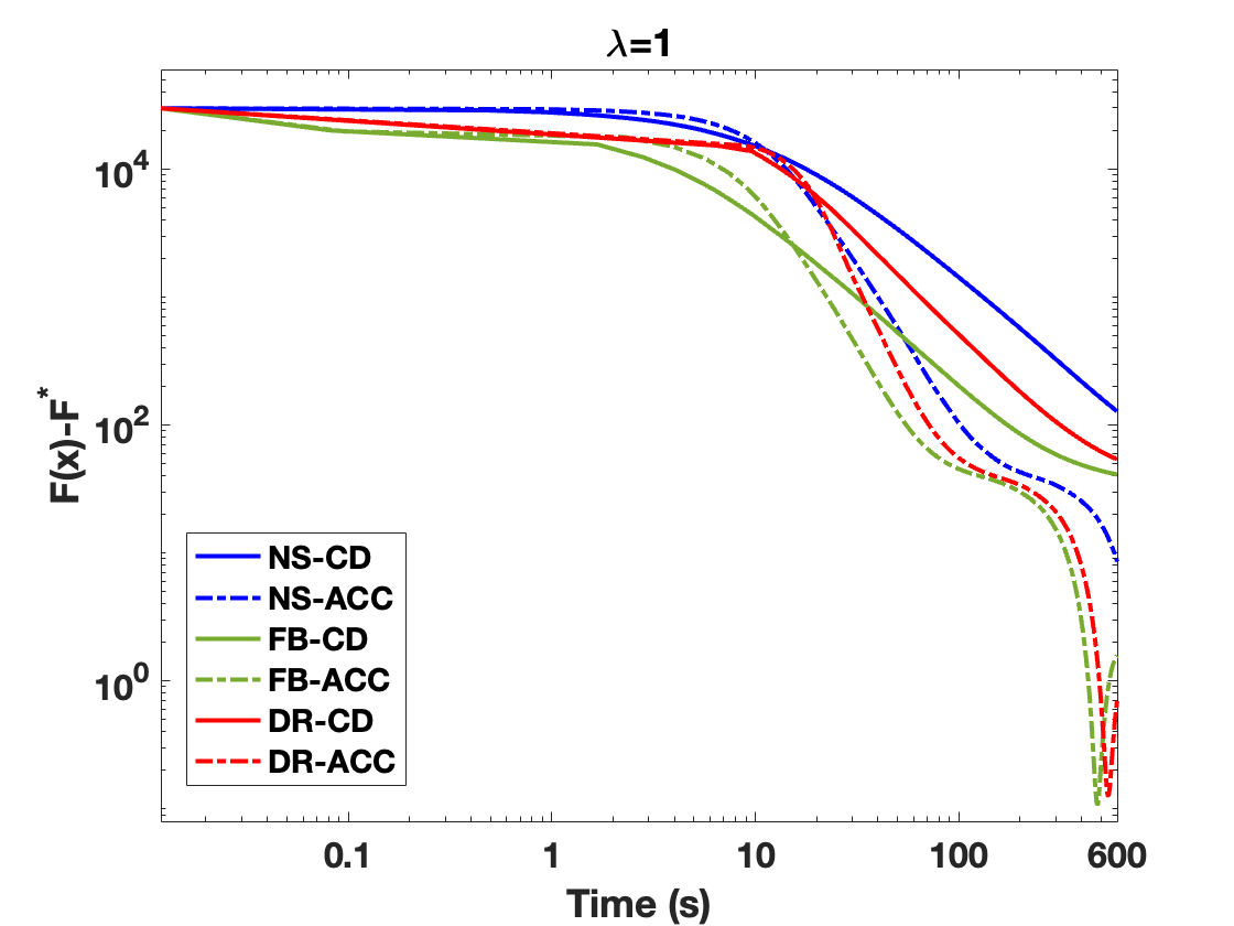
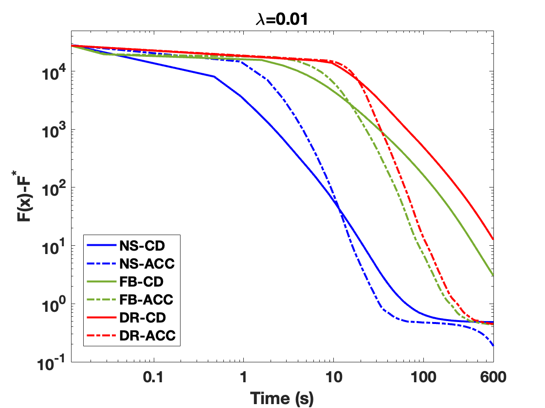
Figure 1: Evolution of Algorithms 1 and 2 for four different smoothing techniques in function values along time for quadratic objective with $\ell_{2}$ regularization and $n=10^{4}$.

6.2 Quadratic objective with TV regularization

We also consider a quadratic problem with TV regularization:

$$\min_{x\in\mathbb{R}^{n}}\dfrac{1}{2}\|Bx-c\|^{2}+\lambda\sum_{i=1}^{n-1}|x^{(i)}-x^{(i+1)}|\vspace{-0.2cm}$$ (83)

with $B\in\mathbb{R}^{n\times n}$ and $c\in\mathbb{R}^{n}$. Vectors $c\in\mathbb{R}^{n}$ and $x_{0}\in\mathbb{R}^{n}$ are generated from a normal distribution $\mathcal{N}(0,1)$ and the matrix $B\in\mathbb{R}^{n\times n}$ is generated as $B=Q^{T}CQ$, where $Q\in\mathbb{R}^{n\times n}$ is a sparse orthogonal matrix and $C\in\mathbb{R}^{n\times n}$ is a diagonal matrix such that $C=\text{diag}(100,\text{rand}(n/2-1,1),\text{zeros}(n/2,1))$. Note that this function satisfies $q$-growth condition with $q=2$. Indeed, consider the function $g:\mathbb{R}^{n}\to\mathbb{R}$ such that $g(y)=\dfrac{1}{2}\|y-c\|$. We have that $g$ is strongly convex with strong convexity paramenter $\sigma_{g}=1$ and the gradient of $g$ is Lipschitz with constant $L_{g}=1$. Moreover $\lambda\sum_{i=1}^{n-1}|x^{(i)}-x^{(i+1)}|$ is a polyhedral function. Hence, from [20, Theorem 10]), the objective function in (83) satisfies $q$-growth condition with $q=2$. Thus, we can also apply Algorithm 3 for solving this problem. We consider the following methods:
1. NS-CD: Nesterov’s smoothing using Algorithm 1.
2. NS-RT: Nesterov’s smoothing using Algorithm 3.
3. FB-CD: Forward-Backward envelope using Algorithm 1.
4. FB-RT: Forward Backward evelope using Algorithm 3.
5. ME-CD: Moreau envelope using Algorithm 1.
6. ME-RT: Moreau evelope using Algorithm 3.
7. PROX: full proximal gradient method.
8. APPROX-RT: full restart accelerated algorithm proposed in [10].

In all restart accelerated algorithms we update the restart periods as in Assumption 4. Moreover, the first restart period is chosen $K_{0}=\lfloor 0.01e\cdot n\rfloor$. We plot the function values along time (in seconds) in Figure 2. As we can see from this figure, Algorithms 1 and 3 on Nesterov’s smoothing are the fastest, with restart accelerated variant having the better performance.

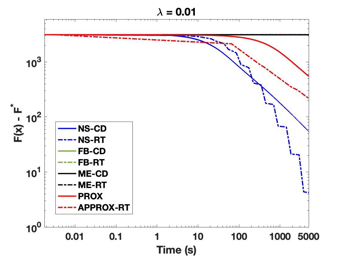
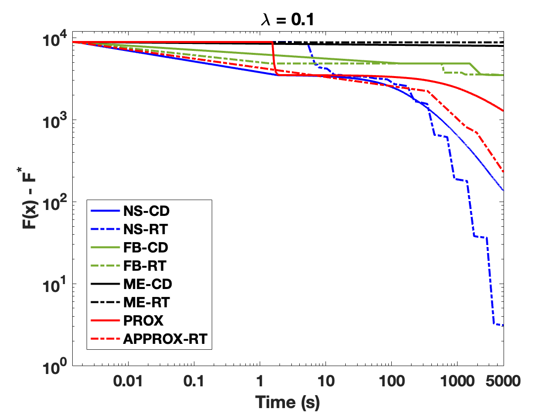
Figure 2: Evolution of Algorithms 1, 3 and their full variants for three different smoothing techniques in function values along time for quadratic objective with TV regularization and $n=10^{4}$.

7 Conclusions

In this paper we have considered a general framework for smooth approximations of nonsmooth and nonseparable objective functions, which covers in particular Moreau envelope, Forward-Backward envelope, Douglas-Rachford envelope and Nesterov’s smoothing. We have derived convergence rates for random (accelerated) coordinate descent methods for minimizing the smooth approximation. Moreover, under an additional $q$-growth assumption on the original function, we have derived improved rates (even linear) for (restart accelerated) coordinate descent variants. We have also introduced a relative randomized coordinate descent algorithm when the original function is relative smooth w.r.t. a (possibly nonseparable) differentiable function. Convergence rates have been also derived for this algorithm in the convex and $q$-growth cases. We have tested our numerical methods on two well-known applications and the numerical results show their efficiency.

Acknowledgments The research leading to these results has received funding from: TraDE-OPT funded by the European Union’s Horizon 2020 Research and Innovation Programme under the Marie Skłodowska-Curie grant agreement No. 861137; UEFISCDI PN-III-P4-PCE-2021-0720, under project L2O-MOC, nr. 70/2022.

Declarations

There is no conflict of interest.

Appendix A

Proof of Lemma 1: Consider $x\in X$ and $h_{0}\in\mathbb{R}^{n_{i}}$, such that $x+U_{i}h_{0}\in X$, fixed. Define the function $r:\mathbb{R}^{n_{i}}\to\mathbb{R}$:

$$r(h)=f(x+U_{i}h)-\langle U_{i}^{T}\nabla f(x+U_{i}h_{0}),h\rangle.$$ (84)

Since $f$ is convex along coordinates, it implies that $r$ is convex. Moreover,

$$\nabla r(h)=U_{i}^{T}\nabla f(x+U_{i}h)-U_{i}^{T}\nabla f(x+U_{i}h_{0}).$$

Hence $h^{*}=h_{0}$ is a optimal point of the function (84). This implies that

$$r(h_{0})\leq r\left(x-\dfrac{1}{L_{i}}U_{i}\nabla r(0)\right).$$

Combining the inequality above with (7), we obtain:

$$f(x+U_{i}h_{0})-\langle U_{i}^{T}\nabla f(x+U_{i}h_{0}),h_{0}\rangle$$

$$\leq f\left(x-\dfrac{1}{L_{i}}U_{i}\nabla r(0)\right)+\dfrac{1}{L_{i}}\langle U_{i}^{T}\nabla f(x+U_{i}h_{0}),\nabla r(0)\rangle$$

$$\leq f(x)+\dfrac{1}{L_{i}}\langle U_{i}^{T}\nabla f(x+U_{i}h_{0})-U_{i}^{T}\nabla f(x),\nabla r(0)\rangle+\dfrac{1}{2L_{i}}\|\nabla r(0)\|^{2}$$

$$=f(x)-\dfrac{1}{L_{i}}\|\nabla r(0)\|^{2}+\dfrac{1}{2L_{i}}\|\nabla r(0)\|^{2}$$

$$=f(x)-\dfrac{1}{2L_{i}}\|\nabla r(0)\|^{2}.$$

This implies that:

$$f(x+U_{i}h_{0})-\langle U_{i}^{T}\nabla f(x+U_{i}h_{0}),h_{0}\rangle+\dfrac{1}{2L_{i}}\|U_{i}^{T}\nabla f(x+U_{i}h_{0})-U_{i}^{T}\nabla f(x)\|^{2}\leq f(x).$$

Exchanging $x$ and $x+U_{i}h_{0}$ in the inequality above and summing up, we obtain:

$$\dfrac{1}{L_{i}}\|U_{i}^{T}\nabla f(x+U_{i}h_{0})-U_{i}^{T}\nabla f(x)\|^{2}\leq\langle U_{i}^{T}\left(\nabla f(x+U_{i}h_{0})-\nabla f(x)\right),h_{0}\rangle.$$

Using the Cauchy-Schwarz inequality, we further get:

$$\|U_{i}^{T}\nabla f(x+U_{i}h_{0})-U_{i}^{T}\nabla f(x)\|\leq L_{i}\|h_{0}\|.$$

Hence, the statement follows.

References

- \bibcommenthead
- Nesterov [2004] Nesterov, Y.: Introductory Lectures on Convex Optimization: a Basic Course. Springer, New York (2004)
- Rockafellar and Wets [1998] Rockafellar, R.T., Wets, R.J.-B.: Variational Analysis. Springer, Berlin (1998)
- Giselsson and Fält [2018] Giselsson, P., Fält, M.: Envelope functions: unifications and further properties. J.Optim. Theory Appl. 178(3), 673–698 (2018)
- Stella et al. [2017] Stella, L., Themelis, A., Patrinos, P.: Forward–backward quasi-newton methods for nonsmooth optimization problems. Comp. Opt. Appl. 67(3), 443–487 (2017)
- Patrinos et al. [2014] Patrinos, P., Stella, L., Bemporad, A.: Douglas-Rachford splitting: complexity estimates and accelerated variants. Conference on Decision and Control (2014)
- Nesterov [2005] Nesterov, Y.: Smooth minimization of non-smooth functions. Mathematical Programming 103, 127–152 (2005)
- Nesterov and Spokoiny [2017] Nesterov, Y., Spokoiny, V.: Random gradient-free minimization of convex functions. Found. Comput. Math. 17, 527–566 (2017)
- Necoara and Fercoq [2022] Necoara, I., Fercoq, O.: Linear convergence of random dual coordinate descent on nonpolyhedral convex problems. Mathematics of Operations Research 47(4), 2547–3399 (2022)
- Necoara and Suykens [2008] Necoara, I., Suykens, J.A.K.: Application of a smoothing technique to decomposition in convex optimization. IEEE Transactions on Automatic Control 53(11), 2674–2679 (2008)
- Fercoq and Qu [2020] Fercoq, O., Qu, Z.: Restarting the accelerated coordinate descent method with a rough strong convexity estimate. Comp. Optim. Appl. 75, 63–91 (2020)
- Fercoq and Richtarik [2015] Fercoq, O., Richtarik, P.: Accelerated, parallel and proximal coordinate descent. SIAM Journal on Optimization 25(4), 1997–2023 (2015)
- Nesterov and Stich [2017] Nesterov, Y., Stich, S.U.: Efficiency of the accelerated coordinate descent method on structured optimization problems. SIAM J. Optim. 27, 110–123 (2017)
- Nesterov [2012] Nesterov, Y.: Efficiency of coordinate descent methods on huge-scale optimization problems. SIAM Journal on Optimization 22(2), 341–362 (2012)
- Aberdam and Beck [2021] Aberdam, A., Beck, A.: An accelerated coordinate gradient descent algorithm for non-separable composite optimization. J. Optim. Theory Appl. (2021) https://doi.org/%****␣Revision1-COAP.bbl␣Line␣225␣****10.1007/s10957-021-01957-1
- Fercoq and Richtárik [2019] Fercoq, O., Richtárik, P.: Smooth Minimization of Nonsmooth Functions with Parallel Coordinate Descent Methods, pp. 57–96. Springer, Cham (2019)
- Lu et al. [2018] Lu, H., Freund, R.M., Nesterov, Y.: Relatively smooth convex optimization by first-order methods, and applications. SIAM J. Optim. 28(1), 333–354 (2018)
- Gao et al. [2021] Gao, T., Lu, S., Liu, J., Chu, C.: On the convergence of randomized Bregman coordinate descent for non-Lipschitz composite problems. International Conference on Acoustics, Speech and Signal Processing, 5549–5553 (2021)
- Hanzely and Richtarik [2021] Hanzely, F., Richtarik, P.: Fastest rates for stochastic mirror descent methods. Comput. Optim. Appl. 79, 717–766 (2021)
- Hien et al. [2022] Hien, L.T.K., Phan, D.N., Gillis, N., Ahookhosh, M., Patrinos, P.: Block Bregman majorization minimization with extrapolation. SIAM J. Opt. 4(1), 1–25 (2022)
- Necoara et al. [2019] Necoara, I., Nesterov, Y., Glineur, F.: Linear convergence of first order methods for non-strongly convex optimization. Math. Program. 175, 69–107 (2019)
- J. Bolte and Suter [2016] J. Bolte, J.P. T. P. Nguyen, Suter, B.W.: From error bounds to the complexity of first-order descent methods for convex functions. Mathematical Programming 165, 471–507 (2016)
- Li and Pong [2018] Li, G., Pong, T.K.: Calculus of the exponent of Kurdyka-Lojasiewicz inequality and its applications to linear convergence of first-order methods. Found. Comput. Math. 18, 1199–1232 (2018)
- Liu and Pong [2017] Liu, T., Pong, T.K.: Further properties of the forward-backward envelope with applications to difference-of-convex programming. Comput. Optim. Appl. 67, 489–520 (2017)
- Yu et al. [2019] Yu, P., Li, G., Pong, T.K.: Deducing Kurdyka-Łojasiewicz exponent via inf-projection. Preprint at https://arxiv.org/abs/1902.03635 (2019)
- Duchi et al. [2008] Duchi, J., Shalev-Shwartz, S., Singer, Y., Chandr, T.: Efficient projections onto the -ball for learning in high dimensions. ICML, 272–279 (2008)
- Barbero and Sra [2014] Barbero, A., Sra, S.: Modular proximal optimization for multidimensional total-variation regularization. Preprint at https://arxiv.org/abs/1411.0589 (2014)
- Johnson [2013] Johnson, N.A.: A dynamic programming algorithm for the fused lasso and l0 - segmentation. J. Comput. Graph. Stat. 22(2), 246–260 (2013)
- Kolmogorov et al. [2016] Kolmogorov, V., Pock, T., Rolinek, M.: Total variation on a tree. SIAM J. Imaging Sci. 9(2), 605–636 (2016)
- Bauschke et al. [2016] Bauschke, H.H., Bolte, J., Teboulle, M.: A descent lemma beyond Lipschitz gradient continuity: first-order methods revisited and applications. Mathematics of Operations Research, 330–348 (2016)
- Chorobura and Necoara [2023] Chorobura, F., Necoara, I.: Random coordinate descent methods for nonseparable composite optimization. SIAM J. Optim. 33(3), 2160–2190 (2023)
- Maulen et al. [2022] Maulen, R., Fadili, S.J., Attouch, H.: An SDE perspective on stochastic convex optimization. Preprint at https://arxiv.org/abs/2207.02750 (2022)
- Stein and Shakarchi [2005] Stein, E.M., Shakarchi, R.: Real Analysis: Measure Theory, Integration, and Hilbert Spaces. Princeton University Press, Princeton, New Jersey (2005)
- Necoara and Chorobura [2021] Necoara, I., Chorobura, F.: Efficiency of stochastic coordinate proximal gradient methods on nonseparable composite optimization. Preprint at https://arxiv.org/abs/2104.13370 (2021)