Epidemiological dynamics in populations structured by neighbourhoods and households

Abstract

Epidemiological dynamics are affected by the spatial and demographic structure of the host population. Households and neighbourhoods are known to be important demographic structures but little is known about the epidemiological interplay between them. Here we present a multi-scale model consisting of neighbourhoods of households. In our analysis we focus on key parameters which control household size, the importance of transmission within households relative to outside of them, and the degree to which the non-household transmission is localised within neighbourhoods. We construct the household reproduction number $R_{*}$ over all neighbourhoods and derive the analytic probability of an outbreak occurring from a single infected individual in a specific neighbourhood. We find that reduced localisation of transmission within neighbourhoods reduces $R_{*}$ when household size differs between neighbourhoods. This effect is amplified by larger differences between household sizes and larger divergence between transmission rates within households and outside of them. However, the impact of neighbourhoods with larger household sizes is mainly limited to these neighbourhoods. We consider various surveillance scenarios and show that household size information from the initial infectious cases is often more important than neighbourhood information while household size and neighbourhood localisation influences the sequence of neighbourhoods in which an outbreak is observed.

[inst1]organization=Department of Mathematical Sciences,addressline=The University of Bath, city=Bath, postcode=BA2 7AY, state=Somerset, country=United Kingdom

Increased localisation of neighbourhood contacts increases the household reproduction number when household size varies between neighbourhoods.

The effect is amplified by larger differences between neighbourhood household sizes and greater emphasis on within-household transmission.

Changes to household size in a given neighbourhood only significantly impact quantities such as the outbreak probability and individual risk of infection locally to that neighbourhood.

Household size information from the initial infectious cases in an outbreak is often more important than neighbourhood information.

In a six neighbourhood model, with neighbourhoods of differing household sizes and strength of localisation of contacts, a clear pattern emerges in the sequence in which neighbourhood infections are observed in a population wide outbreak.

1 Introduction

The spatial demography of a population influences infectious disease epidemiology in numerous ways. Fundamentally, infection spreads via contact between individuals. Who contacts whom is dependent on the spatial arrangement of individuals in the population. Individuals who share the same school, workplace, or household, for example, have a higher probability of contacting one another than those who do not. The same principle applies to those who share the same social groups.

The spatial separation of individuals with respect to where they live is arguably one of the most significant demographic characteristics to account for. Contact rates are likely to be higher between individuals who live in the same community, neighbourhood or household. Moreover, we may observe spatial clustering of households with similar demographic characteristics, such as household size, density, living conditions and wealth into neighbourhoods or communities. For example, a survey in Ile-Ife, Nigeria reported pockets of high household size associated with areas identified as low income [1] and a report on Ulaanbaatar, Mongolia, conducted by World Bank, found that average household size ranges between $3$ and $5$ in different districts of the city [2]. In this paper, we focus on the epidemiological implications of such districts or neighbourhoods based around clusters of similarly sized households. We use a multi-scale model which accounts for contact within-households, within-neighbourhoods and in the wider population to examine how the interplay of transmission patterns at these different scales shapes the epidemiological dynamics. We now briefly review the model paradigms we employ at each scale.

Neighbourhood structure is captured in a metapopulation framework. The basic principle of a metapopulation model is to partition the total population into subpopulations based on their spatial separation. These types of models were first introduced by Levins and subsequently developed by Hanski to study ecological phenomena [3, 4]. They have recently been used to model the emergence of a novel pathogen spreading from a village to a nearby city [5], to model infection spread through a population of villages containing households [6], and the development of multi-scale hierarchical models [7].

In [5], the authors model the emergence of multiple strains of an infectious disease in a rural village. They simulate the model as a stochastic branching process using a Gillespie stochastic simulation algorithm (SSA) and derive the analytic probability of emergence per introduction of the infection to the human population. They then use a metapopulation model to describe the spread of infection to a nearby city via commuters from the village. They derive outbreak size distributions for a range of village population sizes and commuter group sizes. They find that spatial heterogeneity only has a limited effect on the probability of emergence and outbreak size. Our work presented here complements this study by accounting for the finer scale structure of within-household transmission.

In [7] the authors consider a hierarchical stochastic epidemic model which incorporates mixing on multiple scales. Each scale represents a different community grouping, increasing in size, such as neighbourhoods, cities and regions of a country. At any given time an individual in the general population may be assigned to a new local context. Individuals make contact with one another at this level only. The likelihood of two individuals sharing the same local context depends on which level they shared most recently. In this study they found that final size and epidemic duration is highly sensitive to population structure, but $R_{0}$ may not be strongly related to these quantities. Our model has similarities with [7] in that we both consider spatial structure on several scales. However, in our model the structure is more rigid. An individual’s residency remains fixed, we distinguish between within-household and outside of household contacts, and allow individuals to contact others within their own neighbourhoods and beyond it.

Household structure is typically captured in stochastic model frameworks based on small groups of cohabiting individuals. Household models are ideal for distinguishing between transmission within a small well-defined group such as a family and transmission in the wider community. In particular, household structure is important when transmission is strong within the household but weak in the wider community. This is often the case as we usually expect contacts within a household unit to be closer, more frequent and longer. Household models date back to the 1970s [8] and remain an active field of research. They can be formulated in a number of ways. Early work focused on stochastic processes, acknowledging the small number of individuals in the household. Extensive work has been carried out in developing probabilistic frameworks for household models [9, 10, 11] and later in reviewing a range of different reproduction numbers [12, 13]. Branching process theory can be utilised to derive epidemic thresholds.

More recently, stochastic compartment models have been formulated using systems of ordinary differential equations (ODEs), often referred to as master or forward Kolmogorov equations. Here, the state variables define the proportions of households in given epidemiological states and ODEs define the transitions between the possible states [14, 15].

Typical quantities used in the analysis of household models include the early growth rate $r$, the final epidemic size and $R_{*}$. The household reproduction number $R_{*}$ is the average number of households with at least one infected individual resulting from a single infected household in an otherwise susceptible population [16]. Other important quantities include the endemic prevalence of infection among the households and the household offspring distribution — the distribution of the number of secondary infected households resulting from one infectious individual [15]. The expectation of this random variable is $R_{*}$.

Household modelling of epidemics has been a fruitful area of research. In [15] the authors present fundamental theory based on describing the chain of infection within the household as a Markov process. They show that large households can act as amplifiers of infection. This means that large households and strong within household transmission can produce positive epidemic growth, even when transmission outside of households is weak.

In [17] the authors consider a similar model to investigate household-based antiviral treatment during an influenza pandemic. However, they assume a heterogeneous distribution of households and consider several different scenarios of delay before the household antiviral treatment has an impact. They find that effective control of pandemic influenza is highly sensitive to efficient surveillance and administration of antiviral treatment.

The authors of [16] use the same framework to investigate Ebola epidemiology. As in [15], they find that larger household sizes and more intense within-household transmission yield higher $R_{*}$ and other quantifications of epidemic growth and magnitude. In the absence of effective quarantine, the critical probability with which cases need to be detected in order to prevent an epidemic is much higher in communities composed of larger households. This highlights the fundamental importance of demography in epidemiological dynamics.

More recent research has included the effects of demographic change. In [18] the authors find that as fertility decreases, which is often associated with economic development, larger households become rarer but infection incidence increases in these households due to the clustering of susceptibles. In [19] the authors investigate the impact of population demography when infection is endemic. They incorporate both age and household structures with demographic turnover within households as a result of births, deaths or splitting. They find that age-structured connectivity increases infection through assortativity, while household structure reduces it. These two structures act synergistically to amplify infection concentration in large households with a majority of young people [19].

2 Model Formulation

Figure 1: Schematic of the two neighbourhood model. There are two levels of connectivity: contacts within households and contacts outside of households either with individuals from an individual’s own neighbourhood or from another neighbourhood.

We consider a model composed of $K$ neighbourhoods, in each of which the population is organised into households (see Figure 1). In this study, the total population size in neighbourhood $i$ is $N_{i}=N$, for $i=1,\ldots K$. The household size in neighbourhood $i$ is denoted $n_{i}$. This parameter may vary between neighbourhoods. Hence, the total population size is the sum of the neighbourhood populations $\sum_{i}N_{i}=\sum_{i}n_{i}h_{i}$, where $h_{i}$ denotes the number of households in neighbourhood $i$. In our framework, contact occurs at two scales. All contact rates are frequency dependent. Individuals make contact with members of their household at rate $\beta$. This parameter takes the same value in all neighbourhoods. Individuals make contact outside of their household at rate $\alpha$. A proportion $\rho_{ii}$ of these contacts are with individuals from their own neighbourhood $i$ and a proportion $\rho_{ij}$ are with individuals from neighbourhood $j$.

2.1 Neighbourhood localisation

We model the localisation of contact within neighbourhoods by expressing $\rho_{ij}$, the proportion of contacts an individual from neighbourhood $i$ has with individuals from neighbourhood $j$, in terms of the proportion of contacts which are ‘reserved’ for individuals from their ‘home’ neighbourhood, $r_{i}$ [20]. Contacts outside of the home neighbourhood are then allocated proportionally to the neighbourhood sizes such that

$$\rho_{ii}=r_{i}+(1-r_{i})\frac{\alpha(1-r_{i})N_{i}}{\sum_{k}\alpha(1-r_{k})N_{k}}=r_{i}+(1-r_{i})\frac{(1-r_{i})N_{i}}{\sum_{k}(1-r_{k})N_{k}},$$

and

$$\rho_{ij}=(1-r_{i})\frac{(1-r_{j})N_{j}}{\sum_{k}(1-r_{k})N_{k}},$$

where the sums are over $k=1,\ldots K$. Proportional mixing between the neighbourhoods corresponds to $r_{i}=0$ for all neighbourhoods. In this case no contacts are reserved exclusively for an individual’s home neighbourhood. If all neighbourhoods are of equal size, $\rho_{ii}=\rho_{ij}=1/K$, where $K$ is the number of neighbourhoods. Complete isolation of neighbourhoods corresponds to $r_{i}=1$. In this case all contacts are reserved for their own neighbourhood. Varying $r_{i}$ from $0$ to $1$ increases the neighbourhood contact localisation from proportional mixing to complete isolation.

2.2 Households

The household populations are structured according to the deterministic framework of [14, 16]. Here, each individual in the household is categorised by their disease state: susceptible $(s)$, infectious $(i)$ or recovered $(r)$. Demographic processes are omitted. The state or configuration of a household $(s,i,r)$ is then defined by the number of individuals in the household in each disease state. The set of all possible household states in neighbourhood $j$ is $\mathcal{S}_{j}=\{(s,i,r)|0\leq s,i,r\leq n_{j}\text{\;and\;}s+i+r=n_{j}\}$ [16]. We define $\mathcal{A}$ to be the set of all absorbing household states; household states that have no infectious inhabitants.

A household transitions from one state to another when either (1) a household member becomes infected or (2) an infected household member recovers. Infectious individuals recover at rate $\gamma$. Transmission of infection can occur through either contact within the household or contact outside of the household. Hence, the force of infection acting on a susceptible individual from a household in neighbourhood $i$ is $\alpha(\rho_{ii}I_{i}+\sum_{j}\rho_{ij}I_{j})+\frac{\beta i}{s+i+r-1}$ where $I_{j}$ is the proportion of the population in neighbourhood $j$ that is infected. We explain the construction of the transmission rate in Section 2.4. We model the transmission process within the household as a continuous-time Markov process (CTMP) [15]. We let $q(k,l)$ be the rate of transition from household state $k$ to state $l$ if $k\neq l$ and $q(k,k)=-\sum_{k\neq l}q(k,l)$. These transition rates form the elements of the Markovian transition matrix $Q$ [16]. The rates of all possible transitions between states are shown in Table 1.

Table 1: Transition rates from household state $k$ to state $l$ (for a household in neighbourhood $1$). The transition due to infection can occur by transmission within the household, or outside of it.

State $k$	State $l$	Transition	Rate $q(k,l)$
$(s,i,r)$	$(s-1,i+1,r)$	infection	$\alpha s(\rho_{11}I_{1}+\sum_{j}\rho_{1j}I_{j})+\frac{\beta si}{s+i+r-1}$
$(s,i,r)$	$(s,i-1,r+1)$	recovery	$\gamma i$

2.3 Households of size 1

Here we generate some insight into the neighbourhood structure by considering a model with two neighbourhoods composed of households of size $1$. So $n_{1},n_{2}=1$. We denote the total proportions of susceptible, infectious and recovered individuals in neighbourhood $i$ by $S_{i}$, $I_{i}$ and $R_{i}$ respectively. Then

$$\begin{split}\frac{dS_{1}}{dt}&=-\alpha\left(\rho_{11}I_{1}+\rho_{12}I_{2}\right)S_{1},\\ \frac{dS_{2}}{dt}&=-\alpha\left(\rho_{22}I_{2}+\rho_{21}I_{1}\right)S_{2},\\ \frac{dI_{1}}{dt}&=\alpha\left(\rho_{11}I_{1}+\rho_{12}I_{2}\right)S_{1}-\gamma I_{1},\\ \frac{dI_{2}}{dt}&=\alpha\left(\rho_{22}I_{2}+\rho_{21}I_{1}\right)S_{2}-\gamma I_{2},\\ \frac{dR_{1}}{dt}&=\gamma I_{1},\\ \frac{dR_{2}}{dt}&=\gamma I_{2}.\end{split}$$ (1)

The total population size remains constant and $S_{i}+I_{i}+R_{i}=1$ for $i=1,2$. The total number of contacts per unit time individuals from neighbourhood $i$ make with individuals from neighbourhood $j\neq i$ must be equal to the number of contacts individuals from neighbourhood $j$ make with individuals from neighbourhood $i$. Therefore $\rho_{12}N_{1}=\rho_{21}N_{2}$, where $N_{1}$ and $N_{2}$ are the respective population sizes of neighbourhoods $1$ and $2$. We assume $\alpha$ is the same for both neighbourhoods.

The basic reproduction number for this model, found using next generation methods [21], is $R_{0}=\frac{\alpha}{2\gamma}\left[(\rho_{11}+\rho_{22})+\sqrt{(\rho_{11}+\rho_{22})^{2}-4(\rho_{11}\rho_{22}-\rho_{12}\rho_{21})}\right]$. Clearly, under proportional mixing and when neighbourhoods are of equal size, $\rho_{11}=\rho_{12}=\rho_{21}=\rho_{22}=1/2$ and the reproduction number reduces to $R_{0}=\alpha/\gamma$. However, when mixing is not proportional the neighbourhood structuring influences $R_{0}$.

Therefore, in the absence of household structure, neighbourhood localisation of contact can influence the epidemic risk and the expected numbers of infections in the early generations of an epidemic.

2.4 Households of size $n>1$

For two neighbourhoods $j=1,2$ with households of fixed size $n_{j}$, we can describe the epidemiological dynamics in the population as a whole using the single household approximation [14, 16, 22] given by the system of ordinary differential equations (ODEs):

$$\begin{split}\dot{H}^{j}_{sir}&=\alpha(\rho_{jj}I_{j}+\rho_{jk}I_{k})\left[-sH^{j}_{sir}+(s+1)H^{j}_{(s+1)(i-1)r}\right]\\ &+\beta\left[-s\frac{i}{n_{j}-1}H^{j}_{sir}+(s+1)\frac{i-1}{n_{j}-1}H^{j}_{(s+1)(i-1)r}\right]\\ &+\gamma\left[-iH^{j}_{sir}+(i+1)H^{j}_{s(i+1)(r-1)}\right].\end{split}$$ (2)

Here, $H^{j}_{sir}$ denotes the probability that a household is in neighbourhood $j$ in state $(s,i,r)$ and $I_{j}=\frac{\sum_{\mathcal{S}_{j}}i\cdot H_{sir}^{j}}{n_{j}}$ is the proportion of individuals in neighbourhood $j$ that are infected at time $t$. Other household states and proportions are denoted analogously. In system (2) we adopt the convention that any states generated on the right hand side of the ODEs that are not contained in $\mathcal{S}_{j}$ for $j=1,2$ are set to zero. For example, for states with either $s,i,r<0$, the proportion of households in these states is automatically zero. The terms in the square brackets correspond to transmission outside of the household, transmission within the household and recovery respectively.

The terms for transmission outside of the household involve several variables. Each of the $s$ susceptibles in a given household contacts individuals from the wider community at rate $\alpha$. Transitions between household state $(s,i,r)$ and $(s-1,i+1,r)$ (labelled states $j$ and $k$ respectively) due to transmission outside of the household occur at rate $\alpha s(\rho_{jj}I_{j}+\rho_{jk}I_{k})$. Within a household, each of the $s$ susceptible individuals contacts other individuals in the household at rate $\beta$. A proportion $i/(n_{j}-1)$ of these contacts are with infectious individuals. Hence the within-household transmission rate for neighbourhood $j$ is $\beta si/(n_{j}-1)$.

2.5 Calculating $R_{*}$

The household reproduction number $R_{*}$ is defined as the expected number of households infected by a single infectious household, in an otherwise susceptible population [16]. Closed form expressions for $R_{*}$ for a single neighbourhood of households of size $2$ or $3$ can be found; see Supplementary (Section $1$).

However, for large household sizes and multiple neighbourhoods, expressions for $R_{*}$ become more complex. We therefore calculate $R_{*}$ for general household sizes $n_{j}$ using the transition matrix $Q$ for the within-household model. Full details of this construction are given in [15]; however, we will briefly explain the concept below.

To obtain the expected number of infected households originating from a single infectious household, we average over all neighbourhoods weighted in proportion to the stable ratio in the exponential growth phase of the epidemic. For two neighbourhoods this corresponds to taking the spectral radius of the next generation matrix $K$ [21],

$$K=\begin{pmatrix}R^{11}_{*}&R^{12}_{*}\\ R^{21}_{*}&R^{22}_{*}\end{pmatrix},$$ (3)

where $R^{ij}_{*}$ is the expected number of infected households in neighbourhood $j$ arising from a single primary infected household in neighbourhood $i$ in an otherwise susceptible population.

$R^{11}_{*}$, for example, can be written as $\frac{\alpha\rho_{11}}{\gamma}H^{1,\infty}_{j}$. Here, $H^{1,\infty}_{j}$ is the expected household epidemic size (of a household in neighbourhood 1), where initially there is one infected individual in the household (state $j=n_{1}-1,1,0$). Following [16], we can write $H^{1,\infty}_{j}$ as $\gamma e^{1}_{j}$, where $e^{1}_{j}$ is the expectation of the path-integral $\Gamma=\int_{0}^{\infty}f(X(t))dt$ conditional on the Markov process starting in state $j$. Here $X(t)$ is the CTMP that describes the infection process within the given household and $f(j)$ maps the household state $j$ to the number of infectious individuals in that state $j$. So $f(j)=i$ when $j$ is state $(s,i,r)$. Each time a new individual becomes infected within the household, the expected reward increases by $1/\gamma$, the expected infectious period. Consequently, the expected household epidemic size for a household in neighbourhood $1$, starting in state $j=n_{1}-1,1,0$, is $H^{1,\infty}_{j}=\gamma e^{1}_{j}$ [15, 16]. The expected number of infections an infected individual in neighbourhood 1 produces outside of their own household but within their home neighbourhood is $\alpha\rho_{11}/\gamma$. We assume that each of these infections involves someone from a different household. Following [15], we find $e^{1}_{j}$ by solving the following system of linear equations

$$\sum_{k\in\mathcal{C}_{1}}q^{1}(j,k)e^{1}_{k}+f(j)=0,\;\;\;j\in\mathcal{C}_{1}.$$ (4)

In equations (4), $\mathcal{C}_{1}$ denotes the set of all transient states for a household in neighbourhood $1$; $q^{1}(j,k)$ is the rate of transition from household state $j$ to $k$ in neighbourhood $1$ and $f(j)$ is defined as above.

In conclusion, the expected number of infected households in neighbourhood $1$ arising from one infected household in neighbourhood $1$ is

$$R^{11}_{*}=\frac{\alpha\rho_{11}}{\gamma}H^{1,\infty}_{j}=\frac{\alpha\rho_{11}}{\gamma}\gamma e_{j}^{1}=\alpha\rho_{11}e_{j}^{1}.$$

Similar considerations give

$$R^{12}_{*} =e^{1}_{j}\alpha\rho_{12}=e^{1}_{j}\alpha(1-\rho_{11}),$$

$$R^{21}_{*} =e^{2}_{j}\alpha\rho_{21}=e^{2}_{j}\alpha(1-\rho_{22}),$$

$$R^{22}_{*} =e^{2}_{j}\alpha\rho_{22}.$$

2.6 Probability of an outbreak

2.6.1 A single neighbourhood

Consider the branching process for the single neighbourhood model. Under a branching process framework there are two possible outcomes: the outbreak becomes extinct with probability $1$ or there is a positive probability that the number of infections grows without bound [21, 23]. We define the probability of a major outbreak as the probability that the branching process does not become extinct (for a given initial condition on the number of infected individuals in the neighbourhood(s)). For a single neighbourhood population, the major outbreak probability can be derived relatively easily using branching process theory [21, 23, 24]. In this case, the branching process, originating from a single infectious individual, dies out with probability $p$. This is the minimal non-negative solution of the equation $G(p)=p$. So $1-p$ is the probability of a major outbreak. Here, $G(p)=\sum_{k=0}^{\infty}p^{k}g(k)$ is the offspring probability generating function and $g(k)$ is the probability that a primary infectious household produces $k$ secondary infectious households.

These probabilities correspond to the offspring distribution for the given household of size $n$. Closed form expressions for the offspring distribution are relatively easy to obtain for households of size $1$ and $2$; see Supplementary (Section $2$). For larger household sizes we find the offspring distribution numerically. This involves solving a system of linear equations [25, 15] in order to obtain the Laplace Stieltjes transform (LST) $y_{i}(s)=\mathbbm{E}[\exp{(-s\alpha\Gamma)}|X(0)=i]$ of the path-integral $\Gamma$ for $i$ in the set of all transient household states $\mathcal{C}$. This is the same path-integral as in Subsection 2.5; remember that $X(t)$ is the CTMP that describes the infection process within the household and $i$ is the initial state of the household. The system of linear equations is

$$\sum_{j\in\mathcal{S}}q(i,j)y_{j}(s)=s\alpha f(i)y_{i}(s),\;\;\;i\in\mathcal{C}.$$ (5)

As previously, $q(i,j)$ represents the rate of transition from household state $i$ to $j$ for a single neighbourhood model. The set of all household states is $\mathcal{S}$ and $\mathcal{C}$ denotes the set of all the transient household states. From this, the required offspring distribution can be constructed recursively by noting that $g(k)=(-1)^{k}\frac{y_{1}^{k}(1)}{k!}$ and we can obtain the $k\textsuperscript{th}$ derivative of $y_{1}(s)$ with respect to $s$ by differentiating system (5) [15].

Under the branching process framework, we assume an infinite population of households. In consequence, each new infection outside of a household occurs in a fully susceptible household that has not been previously infected. This approximation is reasonable in the early stages of an outbreak.

2.6.2 Two neighbourhoods

For the two neighbourhood model, we construct a multi-type branching process of neighbourhood $1$ and neighbourhood $2$ households. Let $X_{1}(t)$ be the CTMP describing the infection process occurring within a household in neighbourhood $1$. We define $\Lambda_{11}$ as the total force of infection on households in neighbourhood $1$ over the course of the household epidemic from neighbourhood $1$:

$$\Lambda_{11}=\int^{\infty}_{0}f_{1}(X_{1}(t))dt.$$

$f_{1}(X_{1}(t))$ is the rate at which a household in neighbourhood $1$ infects other households in neighbourhood $1$ (conditional on the initial state of the Markov process). $\Lambda_{12}$ is defined analogously,

$$\Lambda_{12}=\int_{0}^{\infty}f_{2}(X_{1}(t))dt.$$

This is the total force of infection experienced by households in neighbourhood $2$ over the course of the household epidemic from neighbourhood $1$. The joint LST of $(\Lambda_{11},\Lambda_{12})$, conditioned on the initial household state, $IC_{1}=(s=n_{1}-1,i=1,r=0)$, is the total force of infection outside of the household over the course of the (neighbourhood $1$) household epidemic [26]. This is

$$y_{j}^{1}(s_{1},s_{2})=\mathbbm{E}\left[\exp{(-s_{1}\Lambda_{11}-s_{2}\Lambda_{12})}|X_{1}(0)=j\right],$$ (6)

where $j=IC_{1}$ is the initial household state.

Adapting the results of the path-integral methods used in [25, 15, 26] it follows that,

$$\sum_{j\in\mathcal{S}_{1}}q^{1}(i,j)y_{j}^{1}(s_{1},s_{2}) =(f_{1}(i)s_{1}+f_{2}(i)s_{2})y_{i}^{1}(s_{1},s_{2})$$ (7)

$$=\alpha(\rho_{11}s_{1}+\rho_{12}s_{2})I(X_{1}=i)y_{i}^{1}(s_{1},s_{2}),\;\;\;\forall i\in\mathcal{C}_{1}.$$ (8)

$q^{1}(i,j)$, $\mathcal{S}_{1}$ and $\mathcal{C}_{1}$ are defined as in Subsection 2.5. The function $I(X_{1}=i)$ is used to denote the number of infectious individuals in the household when the CTMP is in state $i$.

Let the probability that a chain of infection starting from a single individual of type $m$ becomes extinct be $p_{m}$. Then in a multi-type branching process of two types, $p_{m}$ is the minimal non-negative solution to the system of equations

$$p_{m}=G_{m}(p_{1},p_{2}),\;\;\;m=1,2,$$

where $G_{m}$ is the offspring probability generating function of an individual of $m\textsuperscript{th}$ type. For the neighbourhood $1$ type, the generating function is

$$G_{1}(z_{1},z_{2})=\sum_{k_{1}=0}^{\infty}\sum_{k_{2}=0}^{\infty}z_{1}^{k_{1}}z_{2}^{k_{2}}g(k_{1},k_{2}),$$ (9)

where $g(k_{1},k_{2})$ is the probability of $k_{1}$ and $k_{2}$ newly infected households in neighbourhoods $1$ and $2$ respectively arising from the household epidemic in a single infected household in neighbourhood $1$. This probability can be written as

$$g(k_{1},k_{2})=\int_{0}^{\infty}\int_{0}^{\infty}\eta_{1}(\lambda_{1},\lambda_{2})\frac{\exp{(-\lambda_{1})}\lambda_{1}^{k_{1}}}{k_{1}!}\frac{\exp{(-\lambda_{2})}\lambda_{2}^{k_{2}}}{k_{2}!}d\lambda_{1}d\lambda_{2},$$ (10)

where $\eta_{1}(\lambda_{1},\lambda_{2})$ is the joint probability density function of the total force of infection (from transmission outside of the households) acting on households in each neighbourhood over the course of the epidemic in the initial infected household in neighbourhood $1$.

If we substitute (10) into (9), we are able to swap the integration and summations in order to achieve

$$G_{1}(z_{1},z_{2})=\int_{0}^{\infty}\int_{0}^{\infty}\eta_{1}(\lambda_{1},\lambda_{2})\exp{(-\lambda_{1}(1-z_{1}))}\exp{(-\lambda_{2}(1-z_{2}))}d\lambda_{1}d\lambda_{2};$$ (11)

remembering also the power series expansion for the exponential function. Therefore, the offspring generating function is equal to $y^{1}_{IC}(1-z_{1},1-z_{2})$, where $IC$ is the initial condition. So the extinction probability when starting with an initial infection in neighbourhood $1$, $p_{1}$, is given by the minimal non-negative solution $(p_{1},p_{2})$ to the system of equations

$$p_{1}=y^{1}_{IC_{1}}(1-p_{1},1-p_{2})\;\;\ \text{and}\;\;\;p_{2}=y^{2}_{IC_{2}}(1-p_{1},1-p_{2}),$$ (12)

where $IC_{1}=(s=n_{1}-1,i=1,r=0)$ and $IC_{2}=(s=n_{2}-1,i=1,r=0)$ for neighbourhoods $1$ and $2$ respectively and $y^{2}$ is defined analogously to $y^{1}$. The set of equations (12) can be solved numerically and the joint LST is obtained by solving the linear system of equations (7) for $(s_{1},s_{2})=(1-p_{1},1-p_{2})$.

This methodology can be generalised to $k$ neighbourhoods, and to different household types within neighbourhoods [26].

2.7 Parameterisation

In the results presented below we use parameter values from the ranges detailed in Table 2. These values are consistent with an acute respiratory infection such as influenza. The contact rates were determined by first fixing $R_{*}$ across the neighbourhoods to $2.4$ (unless stated otherwise). We do this with the aim of creating a ‘level playing field’ for comparison of results. Next we set the parameter $\nu$. This is the ratio of within household contacts to outside of household contacts, such that $\beta=\nu\alpha$. Larger values of $\nu$ correspond to a greater emphasis on the within-household transmission. Finally, we find the required $\alpha$, and hence $\beta$, values.

Table 2: Parameter values used for all numerical results, unless otherwise stated. They are consistent with an acute respiratory infection such as influenza. All rates per day.

Parameter	Meaning	Values used
$n_{i}$	household size in neighbourhood $i$	$2$–$6$
$h_{i}$	no. households in neighbourhood $i$, $\sum_{i=1}^{2}n_{i}h_{i}=5040$	$840$–$2520$
$\alpha$	transmissible contact rate outside of households	$0.25$–$0.3$
$r_{i}$	propn. external contacts reserved for own neigh.	$0$–$1$
$\nu$	ratio of within to outside of household contacts	$1$–$5$
$\beta$	transmissible contact rate within households	$0.3$–$1.29$
$\gamma$	recovery rate	$0.2$
$R_{*}$	household reproduction number	$2.4$

3 Results

3.1 Model analysis

Our model analysis focuses on understanding the impact that three key parameters have on the epidemiological dynamics: household size $n_{i}$, neighbourhood localisation $r_{i}$ and the ratio of within household contacts to outside of household contacts $\nu$. In particular, we investigate how these quantities influence the household reproduction number $R_{*}$, individual infection risk, the probability of an outbreak and the probability that an outbreak is first observed in a given neighbourhood. We also consider the implications of our model for surveillance and control strategies with regards to the importance of accounting for the neighbourhood or household demography of the first cases that are detected.

3.2 How neighbourhood localisation affects $R_{*}$

We begin by investigating how neighbourhood localisation impacts the household reproduction number in a population structured into two neighbourhoods with different household compositions.

Figure 2 shows how $R_{*}$ changes when the localisation of contact outside of households varies from proportional mixing between neighbourhoods to complete isolation. We observe that, when household size differs between the two neighbourhoods, increasing the localisation of transmission increases the expected number of infections arising from a single infected household in the early stages of an outbreak. This effect occurs because increasing the localisation increases the intensity of contact in both the neighbourhoods, including the one with the larger household sizes. Some of the contacts, and thus infections, that would have occurred in the neighbourhood with smaller households are retained in the neighbourhood with larger households. These larger households will, on average, go on to produce more subsequent infections than the smaller households. This effect is more pronounced for larger differences between household sizes. If both neighbourhoods have equal household sizes there is no effect. We observe the same result for a range of $\nu$. For larger $\nu$, i.e. when within household transmission is more important, we observe larger increases in $R_{*}$ when the localisation of the neighbourhoods is increased.

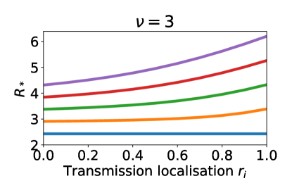
Figure 2: The household reproduction number for a population structured into two neighbourhoods as the localisation of transmission outside of households varies from proportional mixing to complete isolation. Each curve is for a different household size in neighbourhood $1$ ($n_{2}=2$ is fixed). $n_{1}=2,3,4,5,6$ corresponds to the blue, orange, green, red and purple lines respectively. Contact rate parameters are $\alpha=0.27$, $\beta=0.8$, which gives $R_{*}=2.4$ when $n_{1}=2$.

Figure 2 shows the absolute value of $R_{*}$. The parameterisation is such that $R_{*}=2.4$ when $n_{1}=n_{2}$. But increasing $n_{1}$ increases $R_{*}$ independently of transmission localisation. So, to account for the baseline impact of changing $n_{1}$, Figure 3 shows the relative change in $R_{*}$ when neighbourhood $2$ has households fixed at size $2$ and transmission localisation is varied from proportional mixing to complete isolation. When $n_{1}=3$, the relative change in $R_{*}$ for proportional mixing versus isolated neighbourhoods ranges from $11.2$% to $17.4$% for the $\nu$ values we consider. In comparison, when $n_{1}=6$ the relative change in $R_{*}$ ranges from $29.4$% to $45.7$%. The relative change in $R_{*}$ is amplified by larger values of $\nu$ and $n_{1}$.

We observe that weaker localisation of transmission outside of households can significantly reduce the epidemic risk and generation size early in the epidemic, even when the difference in household sizes between the two neighbourhoods is only one.

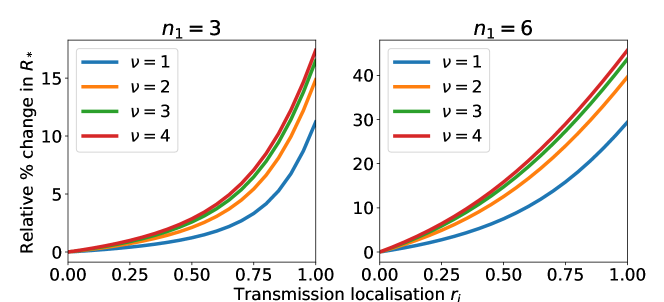
Figure 3: The relative change in the value of the household reproduction number $R_{*}$ in a model with two neighbourhoods as localisation of transmission outside of households varies from proportional mixing between neighbourhoods to complete isolation. In both plots $n_{2}=2$ but household size in neighbourhood $1$ differs. Each curve represents a different ratio of within household contacts to outside of household contacts. $\nu=1,2,3,4$ corresponds to the blue, orange, green and red lines respectively.

3.3 How household size and neighbourhood localisation affects individual infection risk

We define the individual infection risk as the proportion of individuals in the neighbourhood, or in the population as a whole, that have been infected after $100$ days (in our parameter space this corresponds to a time after the outbreak has ended i.e. prevalence is very low and $R_{*}<1$). We calculate this quantity by solving our master equation model (2) over this time period and counting the final number of individuals in the recovered state $r$. We consider the model with two neighbourhoods. Households in neighbourhood $2$ are of size $2$ and we examine how the infection risk depends on the household size in neighbourhood $1$. Figure 46(a) shows the individual infection risk for someone from neighbourhood $2$ (households of size $2$), neighbourhood $1$ (households of size $2$ to $6$) and for someone chosen at random from the population. Localisation corresponds to proportional mixing between neighbourhoods $(r_{i}=0)$. The impact of household size on infection risk is localised. Individual infection risk in neighbourhood $1$ increases from $0.86$ to $0.98$ as household size increases from $2$ to $6$ whereas the increase in individual risk in neighbourhood $2$ is insignificant.

We also consider how the degree of localisation of contacts outside of the household impacts individual infection risk. Figure 46(b) reveals that increasing the neighbourhood localisation of contacts decreases individual infection risk in the neighbourhoods with smaller households but has an insignificant impact on infection risk in the neighbourhoods with larger households.

We conclude that the impact of the household demography of a neighbourhood on infection risk over the entire course of the outbreak is mostly limited to the neighbourhood itself. This contrasts with our previous observation in Figure 3 that increased neighbourhood localisation of contacts outside of the household increases the epidemic risk when there is a difference in household size between the neighbourhoods.

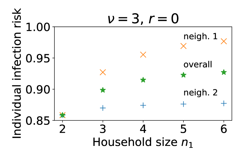
(a)

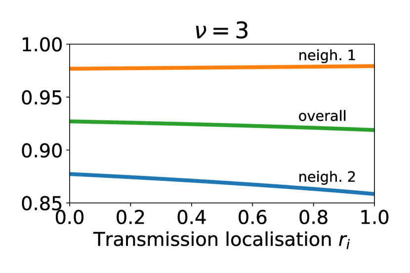
(b)

Figure 4: Individual infection risk over entire outbreak when neighbourhoods have different household sizes and the degree of localisation of neighbourhood transmission is varied. (6(a)) Household size in neighbourhood $1$ is varied from $n_{1}=2$ to $6$. Household size in neighbourhood 2, $n_{2}=2$. Individual infection risks of individuals from neighbourhood $1$, $2$ and overall are shown as blue crosses, orange pluses and green stars respectively. Infection risk is defined as the probability an individual has been infected (and is recovered) by the time the outbreak ends. (6(b)) Households sizes are fixed at $n_{1}=6$ and $n_{2}=2$. The localisation of neighbourhood contacts $r_{i}$ varies from proportional mixing to complete isolation. Infection risk of individuals from neighbourhoods $1$, $2$ and overall are displayed as blue, orange and green curves respectively.

3.4 Outbreak probability and surveillance

In this section we investigate the probability of an outbreak under the $2$ neighbourhoods model framework with respect to neighbourhood household sizes and $\nu$. We further explore how outbreak probability estimates are affected by making different assumptions about the population structure.

We calculated outbreak probabilities by numerical simulation and compared them to the probabilities derived analytically in Section 2.6.2. We used a Gillespie SSA [27] to simulate the infection process among a population of households described by the coupled differential equations in system (2). In the finite simulated population there are often no households in a particular state. So, in order to control the complexity of the simulation, we maintained a dynamic set of household states. We used a dictionary to define the set of all household states present in each neighbourhood at time $t$. Propensity functions were defined for each household state and infection or recovery event. As events occurred, the household dictionary was updated, removing and adding new household states as necessary. All code can be found at https://github.com/ahb48/Neighbourhoods_and_households. Simulation trajectories can show stuttering chains of transmission that die out within a few generations, or sustained periods of transmission with exponential growth patterns. We classify trajectories as representing an ‘outbreak’ if there have been at least $6$ infected households (see Subsection 3.4.1 for further details), and ‘no outbreak’ otherwise.

The analytic and numerical outbreak probability calculations are in good agreement. Figure 5(a) shows that when the initial infected individual is from neighbourhood $1$, increasing the household size within this neighbourhood increases the probability of an outbreak. When $\nu=3$ and mixing is proportionate, for households of size $2$, the outbreak probability is $0.63$ and for households of size $6$ it is $0.78$ (to $2$ decimal places). In comparison, the probability of an outbreak originating from an initial infected individual from neighbourhood $2$ is insensitive to the household composition of neighbourhood $1$ when $n_{2}=2$ remains fixed. The increase in outbreak probability with neighbourhood household size is amplified by larger $\nu$. In Figure 5(b), we see that smaller $\nu$ correspond to outbreak probabilities in neighbourhood $1$ which are less responsive to changes in neighbourhood household size.

Figure 5(c) shows the outbreak probabilities again, together with the outbreak probability calculated using a multi-type branching process approximation that naively assumes a geometric offspring distribution for households of any size. The probability generating functions for the geometric offspring distribution approximation are in the Supplementary (Section $3$). For the specific parameter values used in this figure, the geometric offspring distribution assumption gives a good approximation to the true outbreak probability when $n_{1}=4$ (and $n_{1}=1$, not shown here), but diverges for other values of $n_{1}$.

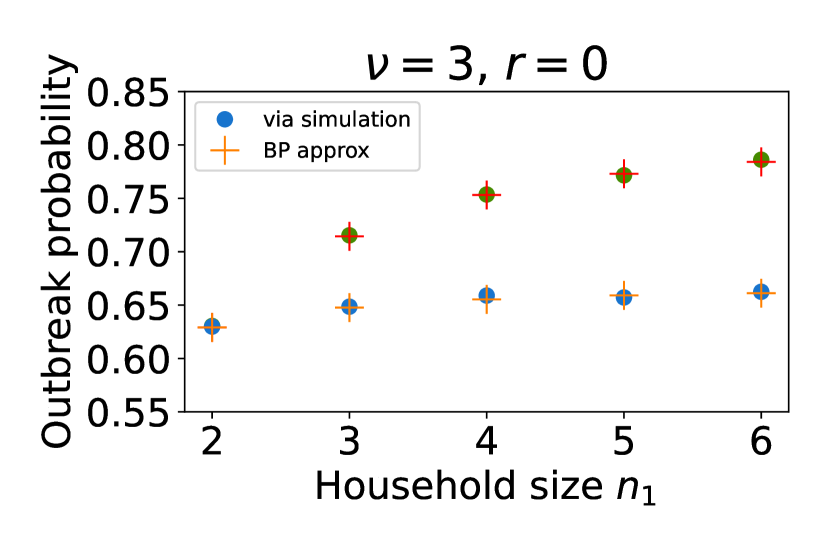
(a)

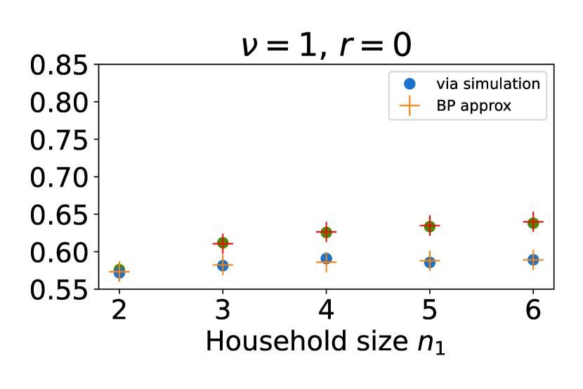
(b)

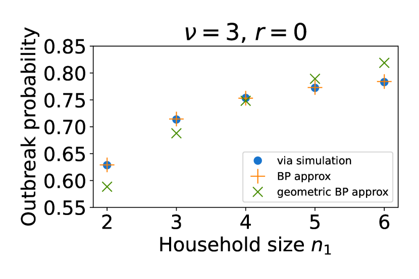
(c)

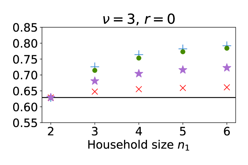
(d)

Figure 5: The probability of an outbreak originating from a single infectious individual in neighbourhood $1$ (higher curve; green dots and red pluses) and a single individual from neighbourhood $2$ (lower curve; blue dots and orange pluses), as we increase the household size in neighbourhood $1$ from $2$ to $6$. Dots denote outbreak probabilities found via $50,000$ Gillespie SSA realisations; pluses denote the multi-type branching process approximation detailed in Subsection 2.6.2. Household size remains fixed at $n_{2}=2$ in neighbourhood $2$ and neighbourhood connectivity is proportionate ($r_{i}=0$). All other parameters are the same as in Table 1 unless stated otherwise. (a) The ratio of within household contacts to outside of household contacts is set to $\nu=3$ and (b) $\nu=1$, and $\alpha,\beta$ are such that $\beta=\nu\alpha$ and $R_{*}=2.4$. (c) Probability of an outbreak originating from a single infectious individual in neighbourhood $1$, as in (a), with for comparison, incorrect branching process approximation based on a geometric offspring distribution shown as green crosses. (d) Probability of an outbreak calculated on the assumption that the initial infectious individual is: from neighbourhood $1$ (greens dots); from neighbourhood $2$ (red crosses); from neighbourhood 1 or 2 with equal probability (purple stars); from a population of households of size $n_{1}$ with no neighbourhood structure (blue pluses). The solid black line denotes the outbreak probability given a single infected individual from a population of households of size $n_{2}=2$ (fixed).

3.4.1 Surveillance

When an infectious disease surveillance system detects one or more cases, we would like to assess whether to expect a short chain of transmission that quickly fizzles out, or a large scale outbreak [28, 29]. Figure 5(d) explores the impact of different demographic assumptions when calculating the probability of a large outbreak on the basis of a small number of initial cases. As before, we assume there is initially a single infected individual in neighbourhood $1$, all households in neighbourhood $2$ are of size $2$, and all households in neighbourhood $1$ are of size $2$ to $6$. Therefore, the true outbreak probability is as in Figure 5(a) (green dots). Now we consider how this probability compares with outbreak probability calculations that do not fully account for the neighbourhood or household structure. If we neglect the neighbourhood structure entirely, and simply assume that all households in the community are of size $n_{1}$, we get a good approximation to the true outbreak probability (blue pluses). However, if we assume that all households in the community are of size $n_{2}$, we get a poor approximation to the true outbreak probability unless $n_{1}=n_{2}$ (shown as black solid line). If we do account for the neighbourhood structure, but incorrectly assume that the initial infected individual is in neighbourhood $2$ then we get a similarly poor approximation to the true outbreak probability (red crosses). If we assume that the initial infected individual has an equal probability of being in each neighbourhood then we get a slightly better approximation (purple stars). This is simply the average of the outbreak probabilities with initial conditions of a single infected individual from neighbourhood $1$ or neighbourhood $2$ respectively. Therefore, we deduce that demographic composition of the neighbourhood where the initial case occurs determines the outbreak probability, almost independently of the demography of the other neighbourhoods, even under proportional mixing.

In Figure 6 we show the error in the various outbreak probability calculations seen in the last column of Figure 5(d) with respect to the number of initial cases. In Figure 5(a), when there is a single case within a household in neighbourhood $1$ ($n_{1}=6$) and it is erroneously assumed that the case originates in a population where all households are of size $n=2$, then the relative percentage error in the outbreak probability is almost $20\%$. The error is similar, Figure 6(b), if the initial case is from neighbourhood $2$ ($n_{2}=2$) but is erroneously assumed to be from a populations where all households are of size $n=6$. When the neighbourhood demography is modelled correctly but the initial case is attributed to the wrong neighbourhood, the relative error in the outbreak probability is slightly lower. When the initial case is attributed to each neighbourhood with equal probability, the relative error is lower in both cases but still $7-10\%$. Finally, if the neighbourhood structure is neglected and all households are assumed to have the same size as that of the initial case then the error is close to $0$ when the initial case is from neighbourhood $1$, close to $5\%$ when it is from neighbourhood $2$. This is due to the additional force of infection associated with larger households in neighbourhood $1$.

As the number of initial infected households increases, the error in each outbreak probability approximation decays exponentially towards $0$. After a chain of $4$ initial cases the errors are negligible. This is because the probability of a major outbreak is much higher (see Figure 7) for all demographic assumptions, reducing the relative scope for error.

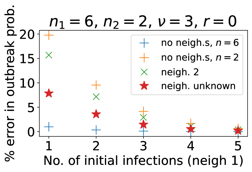
(a)

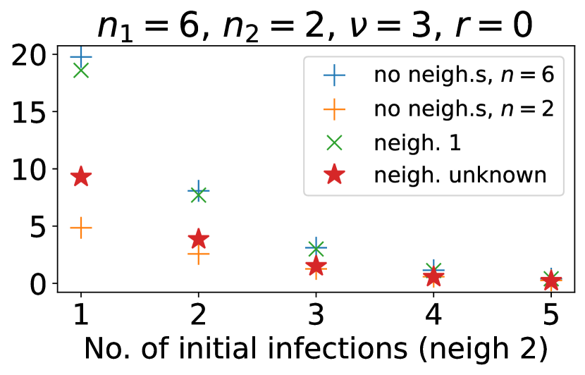
(b)

Figure 6: The relative error in the probability of an outbreak originating from $k=1,2,\ldots,5$ infectious individuals (a) from neighbourhood $1$, $n_{1}=6$ and (b) from neighbourhood $2$, $n_{2}=2$ calculated under various assumptions. Assumptions: population of households size $6(=n_{1})$ with no neighbourhood structure (blue pluses); population of households size $2(=n_{2})$ with no neighbourhood structure (orange pluses); initial infected individuals all in the other neighbourhood (green crosses) and all in unknown neighbourhood (red stars).

3.5 Six neighbourhood model

Here we examine more complex structures by extending our $2$ neighbourhood model to consider $6$ neighbourhoods. We do this to explore how our key parameters, such as household size and the degree to which non-household transmission is localised within neighbourhoods, influence the epidemiological dynamics under more complex neighbourhood structures. Our Gillespie SSA code readily accommodates any number of neighbourhoods. We set up a model composed of six neighbourhoods, two with households of size $2$, two with households of size $4$ and two with households of size $6$. The parameters that control localisation of contact outside of the household in each of these neighbourhoods are randomly assigned such that, in each pair of neighbourhoods, one has weakly localised contacts ($r\sim U[0,0.1]$) and the other has strongly localised contacts ($r\sim U[0.4,0.5]$). See Table 3 for the summary of the $6$ neighbourhood set up. Structuring the model in this way aims to strike a balance between generality and computational tractability. Within this framework we investigate the impact that demographic structure has on the probability that an outbreak is first observed in a given neighbourhood, and the sequence of neighbourhoods in which the outbreak becomes apparent.

Table 3: Six neighbourhood model structure for Figures 8, 9 and 10. $U[a,b]$ denotes that the neighbourhood localisation $r_{i}$ is uniformly distributed over the interval $[a,b]$.

Neighbourhood	$1$	$2$	$3$	$4$	$5$	$6$
Household size	$2$	$2$	$4$	$4$	$6$	$6$
$r_{i}$	$U[0,0.1]$	$U[0.4,0.5]$	$U[0,0.1]$	$U[0.4,0.5]$	$U[0,0.1]$	$U[0.4,0.5]$

We wish to state that an outbreak has been ‘observed’ in a particular neighbourhood. However, a chain of infection can quickly fizzle out, or continue to become a large, observable, outbreak. So detecting a small number of cases in a neighbourhood does not necessarily mean we are observing an outbreak there. Therefore we say that an outbreak is ‘observed’ in neighbourhood when there have been at least $6$ infected households there. We determined this threshold empirically, as follows. We used the Gillespie SSA to simulate $10,000$ realisations of a single neighbourhood model composed of households of size $2$. A realisation was stopped if the number of infections reached zero or $t=100$ days. We classified realisations as a ‘large outbreak’ if a total of $15$ or more households were infected over the course of the infection chain, and ‘insignificant outbreak’ otherwise. Figure 7 shows that a large outbreak occurred in approximately 40% of realisations. However, if we condition on the number of infected households reaching at least 6, then a large outbreak occurred in over 90% of realisations.

Figure 7: The probability $p_{k}$ of a large outbreak occurring after $k$ household infections have been observed. The Gillespie SSA was used to produce $10,000$ realisations of the model with a single neighbourhood composed of households of size $n=2$. Other parameters were $\nu=3$, $\alpha=0.27$ and $\beta=0.8$. A realisation was classified as a large outbreak if it led to a total of at least $15$ infected households.

3.5.1 Neighbourhood in which an outbreak is first observed

Figure 8 shows the probabilities that an outbreak is first observed in neighbourhood $j=1,2,\ldots,6$. The model set up is as described in Section 3.5. The results are based on $500,000$ Gillespie SSA realisations of the model with an initial condition that seeds one infected individual into a randomly selected neighbourhood. So all neighbourhoods have the same probability of being the source of an outbreak. Figures 8(a) and 8(b) show the probability that an outbreak is first observed in each neighbourhood for the ratio of within household contacts to outside of household contacts, $\nu=3$ alone and $\nu=1,3,5$ overlaid for comparison. Outbreaks are more likely to be observed first in neighbourhoods where household sizes are larger, and where contact outside of the household is highly localised.

The probability that the outbreak was first observed in the same neighbourhood as it was seeded are $0.5$, $0.52$ and $0.52$ for the more localised neighbourhoods ($2$, $4$ and $6$), almost independent of household size. Whereas for the less localised neighbourhoods ($1$, $3$ and $5$) the corresponding probabilities are $0.33$, $0.39$ and $0.41$, distinctly dependent on household size. Strong localisation increases the probability that an outbreak is first observed in the same neighbourhood as it was seeded because there are fewer opportunities for the chain of infection to ‘escape’ into other neighbourhoods. When localisation is weaker, household size plays a more important role because rapid transmission in larger households amplifies transmission in the local neighbourhood.

In Figure 8(b), we explore the impact that the ratio of within household contacts to outside of household contacts $\nu$ has on the probability of the first observed neighbourhood outbreak. The height of the overlapping red, blue and purple bars correspond to the respective neighbourhood probabilities when $\nu=1$, $3$, and $5$. For a weaker contact rate within the household (verses contact outside of households i.e. low $\nu$), the amplification effect of large households is smaller, which reduces the probability that an outbreak is first observed in a neighbourhood composed of large households. This effect is most clearly seen in the neighbourhoods that have the smallest and largest household sizes and more localised contacts ($2$ and $6$).

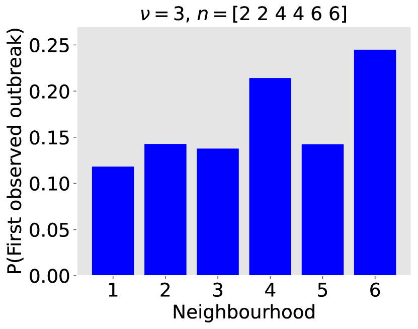
(a)

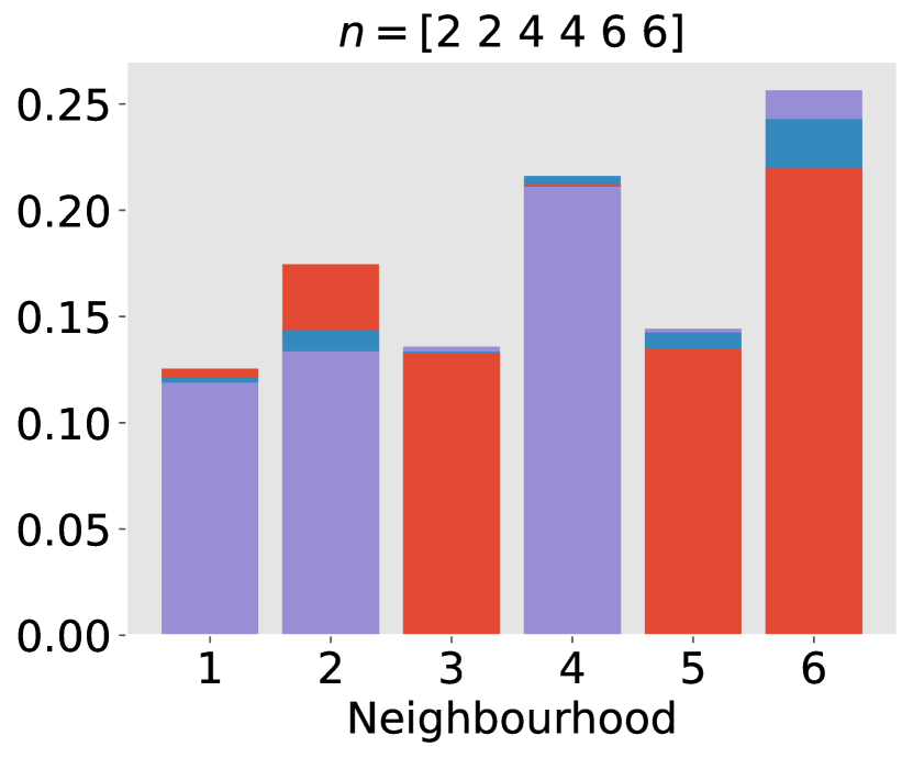
(b)

Figure 8: Probability that an outbreak is first observed in a given neighbourhood. The model has $6$ neighbourhoods. Neighbourhoods $1$ and $2$ have households of size $2$, neighbourhoods $3$ and $4$ have households of size $4$, neighbourhoods $5$ and $6$ have households of size $6$. Neighbourhoods $1$, $3$ and $5$ have weak localisation of contact outside of households. Neighbourhoods $2$, $4$ and $6$ have intermediate localisation. An outbreak is ‘observed’ in a neighbourhood when there have been at least $6$ infected households in that neighbourhood. Outbreak observation probabilities were calculated from $500,000$ Gillespie SSA realisations of the model. For each realisation, the localisation parameters $r_{i}$ were assigned randomly from the distribution $U[0,0.1]$ (neighbourhoods $1$, $3$, $5$) or $U[0.4,0.5]$ (neighbourhoods $2$, $4$, $6$) and the initial condition introduced a single infected individual into a randomly selected neighbourhood. (a) $\nu=3$ (b) $\nu=1,3,5$ in red, blue and purple respectively.

3.5.2 Neighbourhood infection sequences

In addition to considering the neighbourhood in which an outbreak is first observed, we examined the sequence of neighbourhoods in which an outbreak is observed. We seeded trials of the Gillespie SSA with a single infected individual in a random neighbourhood and recorded the order in which neighbourhoods reached the threshold of $6$ infected households. We ran $50,000$ trials with parameter values as in Section 3.5. All trials in which the outbreak did not spread to every neighbourhood were removed, leaving a total of $36,724$ trials in which a significant outbreak occurred.

There are a total of $720$ possible sequences of $6$ neighbourhoods. We calculated the proportion of outbreaks for which each possible sequence was observed. We then used a clustering algorithm to categorise neighbourhood sequences as occurring with high, intermediate or low probability when $\nu=3$. This analysis was carried out using Birch from the ‘sklearn.cluster’ library in Python.

Figure 9 shows that outbreaks were observed in some sequences of neighbourhoods much more frequently than others. The sequences coloured green account for the top $6.9\%$ of trials where significant outbreaks occurred. These trials are made up of $13$ different sequences of neighbourhood infections. The upper dashed line in Figure 9 denotes that sequences above the line occurred in more than $0.46\%$ of trials. The sequences coloured blue occurred in $0.18$-$0.45\%$ of trials. The sequences coloured orange occurred in less than $0.18\%$ of trials, with many of them almost never observed at all. Focusing on the set of sequences that occurred in the top $6.9\%$ of trials, Figure 10 shows the probability that each neighbourhood is the first, second, third etc in which the outbreak is observed. This reveals some insightful patterns. Firstly, these outbreaks are always observed first in neighbourhoods $4$ or $6$. These are the neighbourhoods with households of size $4$ and $6$ with strong localisation of contact outside of the household $r\sim U[0.4,0.5]$. The outbreaks are then usually observed in neighbourhoods $1$, $3$ and $5$. These are the neighbourhoods of size $2$, $4$ and $6$ with weak localisation. Finally, outbreaks are usually observed last in neighbourhoods $2$ and $4$ once again where localisation is stronger. So, in summary, outbreaks tend to be observed first in a strongly localised larger household size neighbourhood because they can gather initial momentum there. They then spread through the less localised (i.e. more connected) neighbourhoods before eventually reaching the remaining highly localised (weakly connected) neighbourhoods.

We observe similar results for a range of values for the ratio of within household contacts to outside of household contacts $\nu$; see Supplementary Figures ($1$ and $2$). The pattern in the most frequently observed sequences of neighbourhood infections becomes less prominent as $\nu$ is decreased since household size becomes less important.

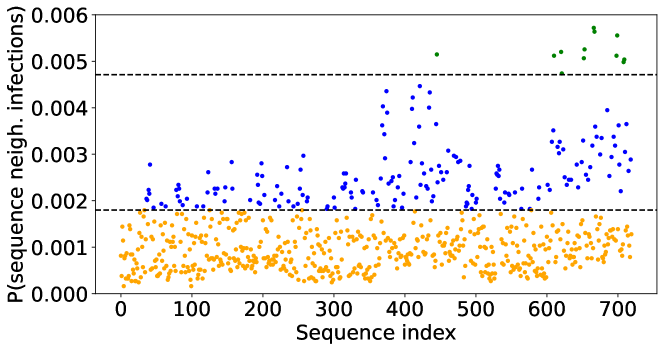
Figure 9: Probability an outbreak is observed in a given sequences of neighbourhoods. There are $720$ possible sequences of $6$ neighbourhoods. Each point in the scatter plot corresponds to a unique sequence and shows the proportion of outbreaks in which the outbreak was observed in that sequence of neighbourhoods. Calculated from $50,000$ Gillespie SSA trials with those that did not result in significant outbreaks discarded. Initially a single individual was infected in a randomly chosen neighbourhood. $\nu=3$ and $r$ is assigned a value from the distribution $U[0,0.1]$ (neighbourhoods $1$,$3$,$5$) or $U[0.4,0.5]$ (neighbourhoods $2$,$4$,$6$). The points above the first dashed line correspond to sequences that occurred in $\geq 0.18\%$ of the outbreaks. Those above the second dashed line occurred in $\geq 0.46\%$ of outbreaks. Clustering was performed with Python using the ‘sklearn.cluster’ library and indicated by colour-coding the points.

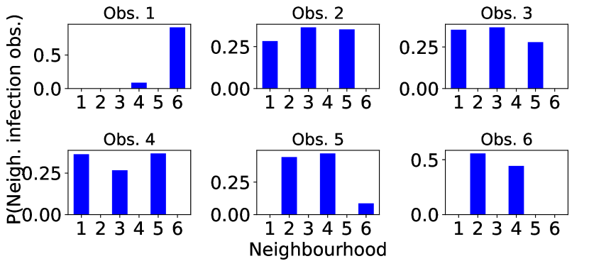
Figure 10: Probability that each neighbourhood is the first, second, third etc in which an outbreak is observed. A total of $50,000$ trials were generated using the Gillespie SSA with a single initial infection in a randomly chosen neighbourhood. Those trials that did not result in significant outbreaks were discarded. Of the remainder, only the top $6.9$% of trials were used to construct this figure. From top left to bottom right the plots correspond to the $1\textsuperscript{st}$, $2\textsuperscript{nd}$, $3\textsuperscript{rd}$, $\ldots$, $6\textsuperscript{th}$ neighbourhood infection to be observed in the sequence of neighbourhood infections. $\nu=3$ and $r$ takes value from either the distribution $U[0,0.1]$ (neighbourhoods $1$,$3$,$5$) or $U[0.4,0.5]$ (neighbourhoods $2$,$4$,$6$).

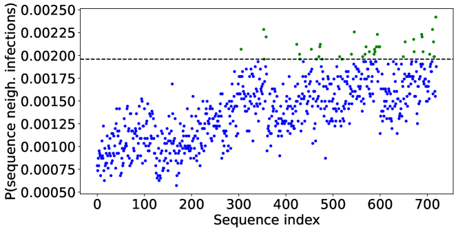
Figure 11: Probability an outbreak is observed through given sequences of neighbourhoods. There are $720$ possible sequences of $6$ neighbourhoods. Each point in the scatter plot corresponds to a unique sequence and shows the proportion of outbreaks in which the outbreak was observed in that sequence of neighbourhoods. Calculated from $50,000$ Gillespie SSA trials with those that did not result in significant outbreaks discarded. Initially a single individual was infected in a randomly chosen neighbourhood. $\nu=3$ and $r$ is assigned a value from the distribution $U[0,0.7]$. The points above the first dashed line correspond to the top $6.9\%$ of the outbreaks.

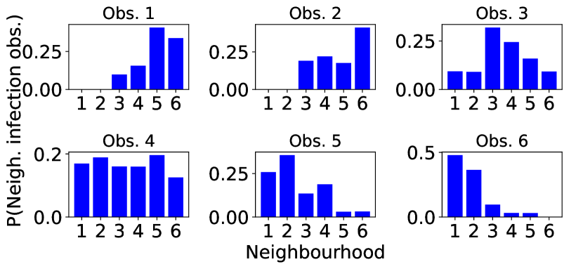
Figure 12: Probability that each neighbourhood is the first, second, third etc in which an outbreak is observed. A total of $50,000$ trials were generated using the Gillespie SSA with a single initial infection in a randomly chosen neighbourhood. Those trials that did not result in significant outbreaks were discarded. Of the remainder, only the top $6.9$% of trials were used to construct this figure. From top left to bottom right the plots correspond to the $1\textsuperscript{st}$, $2\textsuperscript{nd}$, $3\textsuperscript{rd}$, $\ldots$, $6\textsuperscript{th}$ neighbourhood infection to be observed in the sequence of neighbourhood infections. $\nu=3$ and $r$ takes value from the distribution $U[0,0.7]$.

We also examined the neighbourhood sequence in which an outbreak was observed when neighbourhood household sizes were fixed as before but localisation parameters were all assigned entirely randomly from the same distribution. This configuration removes the correlations between household size and localisation. We ran $50,000$ trials and, as before, removed those that did not result in a significant outbreak. This left $36,759$ trials. Figure 11 shows the proportion of outbreaks in which each neighbourhood sequence occurred. Clustering the group of sequences present in the top $6.9\%$ trials where significant outbreaks occurred. We focus on this set of sequences. In comparison to the model with fixed links between household size and localisation, the pattern in the neighbourhood sequences in which the outbreak was observed is weaker; see Figure 12. However, the feature of outbreaks being observed first in neighbourhoods with larger households and last in those with smaller households remains.

Furthermore, the expected value of the localisation parameters $r$ for the $1\textsuperscript{st}$, $2\textsuperscript{nd}$, $3\textsuperscript{rd}$, $\ldots$, $6\textsuperscript{th}$ neighbourhoods observed in the full set of outbreaks was $0.38$, $0.3$, $0.3$, $0.32$, $0.36$ and $0.45$. This once more demonstrates the pattern of outbreaks being observed first and last in more localised neighbourhoods, emerging in the less localised neighbourhoods in between.

4 Discussion

In this paper, we have explored the intertwined role of households and neighbourhoods in the early stages of an epidemic. We built a multi-scale model of a metapopulation of households where contacts can occur both within households and outside of households at different rates. We focused on how several key quantities: neighbourhood household size, localisation, importance of contact within-households relative to contact in the wider community, impacted the dynamics of an infectious disease spreading through this population.

We constructed the household reproduction number $R_{*}$ for the two neighbourhood model. We found that, when neighbourhoods are demographically characterised by different household sizes, greater localisation of community contact increases $R_{*}$. This is because more contacts from the larger household size neighbourhood occur with individuals from their own neighbourhood, leading to a larger number of subsequent chains of infection in the larger households. Larger infected households will on average produce more infections than smaller infected households. Thus, the overall expected number of infected households is larger for greater localisation of contacts. $R_{*}$ is more sensitive to these parameters when the relative importance of within-household contact is higher or there is a bigger difference in the household sizes of the two neighbourhoods.

We derived the analytic probability of a significant outbreak for the two neighbourhood model. We found that increasing the household size of a neighbourhood increases the probability that a single infected individual in that neighbourhood starts an outbreak, but has only a modest impact on the probability of an outbreak originating from a single case in the other neighbourhood. Similarly, an individual’s risk of infection was found to only be impacted locally by household size. Increasing neighbourhood localisation of contacts was shown to decrease individual infection risk in the smaller household size neighbourhood but had little impact on the larger household size neighbourhood.

We investigated the epidemiological dynamics in a model with six neighbourhoods using the Gillespie SSA. We found that population-wide outbreaks are more likely to be detected first in neighbourhoods with more localised community contact. We found considerable stochastic variation in the overall sequence of neighbourhoods in which outbreaks are detected. But, in general, outbreaks tended to be detected first in neighbourhoods with more localised community contact and large households, then neighbourhoods with less localised contact throughout the middle stages, and finally in neighbourhoods with more localised contact but smaller household sizes. This pattern is amplified by increased relative importance of within-household contact.

In the interests of parsimony, and to facilitate interpretation, we fixed parameters in our model such as the local population size, within household contact rate and the recovery rate across all neighbourhoods. We also assumed that household size is homogeneous within any given neighbourhood. In reality, neighbourhood population sizes vary, for example in the city centre versus the suburbs, and there will be a distribution of household sizes within any neighbourhood. These factors will shape the epidemiological dynamics further. Within-household contact rates may vary between neighbourhoods, for instance due to different sanitation systems and building compositions. We chose epidemiological parameters consistent with an acute respiratory infection such as influenza. We were unable to obtain reliable estimates for the within-household contact rates so we set $R_{*}=2.4$ and found the community contact rate $\alpha$ and the within-household contact rate $\beta$ for our chosen values of the relative importance of within-household contact $\nu$. A productive avenue for future work may be to establish more reliable household contact rate estimates from data, or sample the parameter from an empirically motivated distribution as in [17].

This work was inspired by several case studies and city planning documents which highlighted household size to be a key neighbourhood characteristic [2, 1]. When populations are structured in this way, our model may offer some useful insights into infectious disease surveillance and control strategies. We found that, when we wish to estimate the probability of a large outbreak on the basis of a small number of initial cases, household information for those individuals is more useful than knowing the demographic composition of the other neighbourhoods.

This work uses a relatively simple model to provide fundamental insights into the epidemiological implications of multi-scale demographic structures. There are many ways in which this modelling framework can be extended to explore finer details of the demography. We model the neighbourhood localisation of contact by assuming a proportion of an individual’s contacts outside of their own household are ‘reserved’ for other individuals from the same neighbourhood. The remaining non-household contacts can occur at random with any individual from the entire population. Future work may introduce additional information about where these general contacts take place, for instance integrating school and workplace constructs that have already been introduced elsewhere [30].

Our model assumes that all households in a neighbourhood are the same size. But the framework can be easily adapted to incorporate distributions of household sizes and future work may consider more complex demographic structures and evolving population densities. Many countries are now looking to ‘smart growth’ policies [2] in order to accommodate growing populations in urban areas. These policies involve the idea of building upwards rather than outwards. This strategy will increase neighbourhood and community population densities but lead to smaller households and lower family densities within individual houses. These population density changes at different scales may act synergistically to transform the infectious disease epidemiology.

Finally, our analysis assumes that surveillance is always perfect and all cases are detected immediately. In reality, many cases are undetected, there are reporting delays, and there is only partial information about the circumstances of individual cases. Hence future work may examine the impact of such partial information on outbreak predictions. One possible starting point may be recent work on the information content of cross-sectional versus cohort study sampling designs for fixed household sizes [31].

In conclusion, infectious disease epidemiology is shaped by demographic structures at several scales including households and neighbourhoods. Accounting for these structures can lead to a better understanding of epidemic risk and the patterns of epidemic spread and support more robust surveillance strategies.

5 Supplementary information

All code used to produce the results in this piece of work can be found at https://github.com/ahb48/Neighbourhoods_and_households. Supplementary information can be found in a supporting document online.

6 Acknowledgments

This work is supported by a scholarship from the EPSRC Centre for Doctoral Training in Statistical Applied Mathematics at Bath (SAMBa), under the project EP/S022945/1. For the purpose of open access, the author has applied a Creative Commons Attribution (CC-BY) licence to any Author Accepted Manuscript version arising. No new data were created during the study.

References

- [1] M. Ibitoye, O. Akinyemi, S. Adegboyega, A. O. Fabiyi, Spatial analysis of the variations in household living conditions in Ile-Ife, Nigeria, Ife Soc Sci Rev. 25 (1) (2017) 83–97.
- [2] T. Kamata, J. A. Reichert, T. Tsevegmid, Y. Kim, B. Sedgewick, Mongolia-enhancing policies and practices for ger area development in Ulaanbaatar, Tech. rep., The World Bank (2010).
- [3] R. Levins, Some demographic and genetic consequences of environmental heterogeneity for biological control, Am Entomol. 15 (3) (1969) 237–240.
- [4] I. Hanski, Metapopulation dynamics, Nature 396 (6706) (1998) 41–49.
- [5] R. J. Kubiak, N. Arinaminpathy, A. R. Mclean, Insights into the evolution and emergence of a novel infectious disease, PLoS Comp Biol. 6 (9) (2010) e1000947.
- [6] T. Britton, T. Kypraios, P. D. O’Neill, Inference for epidemics with three levels of mixing: methodology and application to a measles outbreak, Scand J Stat. 38 (3) (2011) 578–599.
- [7] D. J. Watts, R. Muhamad, D. C. Medina, P. S. Dodds, Multiscale, resurgent epidemics in a hierarchical metapopulation model, Proc Natl Acad Sci. 102 (32) (2005) 11157–11162.
- [8] R. Bartoszyński, On a certain model of an epidemic, Appl Math. 2 (13) (1972) 139–151.
- [9] F. Ball, D. Mollison, G. Scalia-Tomba, Epidemics with two levels of mixing, Ann Appl Probab. (1997) 46–89.
- [10] F. Ball, O. D. Lyne, Stochastic multi-type SIR epidemics among a population partitioned into households, Adv Appl Probab. 33 (1) (2001) 99–123.
- [11] F. Ball, P. Neal, A general model for stochastic SIR epidemics with two levels of mixing, Math biosci. 180 (1-2) (2002) 73–102.
- [12] L. Pellis, F. Ball, P. Trapman, Reproduction numbers for epidemic models with households and other social structures. I. definition and calculation of R0, Math biosc. 235 (1) (2012) 85–97.
- [13] F. Ball, L. Pellis, P. Trapman, Reproduction numbers for epidemic models with households and other social structures II: comparisons and implications for vaccination, Math biosci. 274 (2016) 108–139.
- [14] T. House, M. J. Keeling, Deterministic epidemic models with explicit household structure, Math biosci. 213 (1) (2008) 29–39.
- [15] J. V. Ross, T. House, M. J. Keeling, Calculation of disease dynamics in a population of households, PLoS One 5 (3) (2010) e9666.
- [16] B. Adams, Household demographic determinants of Ebola epidemic risk, J Theor Biol. 392 (2016) 99–106.
- [17] A. J. Black, T. House, M. J. Keeling, J. V. Ross, Epidemiological consequences of household-based antiviral prophylaxis for pandemic influenza, J R Soc Interface 10 (81) (2013) 20121019.
- [18] N. Geard, K. Glass, J. M. McCaw, E. S. McBryde, K. B. Korb, M. J. Keeling, J. McVernon, The effects of demographic change on disease transmission and vaccine impact in a household structured population, Epidemics 13 (2015) 56–64.
- [19] J. Hilton, M. J. Keeling, Incorporating household structure and demography into models of endemic disease, J R Soc Interface 16 (157) (2019) 20190317.
- [20] J. A. Jacquez, C. P. Simon, J. Koopman, L. Sattenspiel, T. Perry, Modeling and analyzing HIV transmission: the effect of contact patterns, Math Biosci. 92 (2) (1988) 119–199.
- [21] O. Diekmann, J. A. P. Heesterbeek, Mathematical epidemiology of infectious diseases: model building, analysis and interpretation, Vol. 5, 2000.
- [22] A. Holmes, M. Tildesley, L. Dyson, Approximating steady state distributions for household structured epidemic models, Journal of Theoretical Biology 534 (2022) 110974.
- [23] K. Athreya, P. Ney, Branching processes, New York (1972).
- [24] A. L. Lloyd, J. Zhang, A. M. Root, Stochasticity and heterogeneity in host–vector models, J R Soc Interface 4 (16) (2007) 851–863.
- [25] P. Pollett, V. Stefanov, Path integrals for continuous-time Markov chains, J appl probab. 39 (4) (2002) 901–904.
- [26] J. V. Ross, A. J. Black, Contact tracing and antiviral prophylaxis in the early stages of a pandemic: the probability of a major outbreak, Math Med Biol. 32 (3) (2015) 331–343.
- [27] D. T. Gillespie, Exact stochastic simulation of coupled chemical reactions, J Phys Chem. 81 (25) (1977) 2340–2361.
- [28] N. Arinaminpathy, A. McLean, Evolution and emergence of novel human infections, Proceedings of the Royal Society B: Biological Sciences 276 (1675) (2009) 3937–3943.
- [29] E. Southall, Z. Ogi-Gittins, A. Kaye, W. Hart, F. Lovell-Read, R. Thompson, A practical guide to mathematical methods for estimating infectious disease outbreak risks, Journal of Theoretical Biology (2023) 111417.
- [30] L. Pellis, N. M. Ferguson, C. Fraser, Threshold parameters for a model of epidemic spread among households and workplaces, J R Soc Interface 6 (40) (2009) 979–987.
- [31] T. M. Kinyanjui, L. Pellis, T. House, Information content of household-stratified epidemics, Epidemics 16 (2016) 17–26.