Translational eigenstates of He@C60 from four-dimensional ab initio Potential Energy Surfaces interpolated using Gaussian Process Regression

Abstract

The endofullerene system He@C60 has been recently synthesised and characterised experimentally and its spectra were self-consistently assigned quantum mechanically by fitting a one-dimensional radial potential. While this described the majority of the observed data, the one-dimensional model neglects any angular dependence in the potential, and the possible effect of the cage breathing mode. We investigate the importance of these effects with a four-dimensional Potential Energy Surface (PES): three He translational degrees of freedom and C60 cage radius.

We compare MP2, SCS-MP2, SOS-MP2 and RPA@PBE to calibrate and gain confidence in the choice of electronic structure method. Due to the high cost of these calculations, the PES is interpolated using Gaussian Process Regression (GPR), owing to its effectiveness with sparse training data. The PES is split into a two-dimensional radial surface, to which corrections are applied to achieve an overall four-dimensional surface. We find that the quality of PES is very sensitive to the choice of kernel and metric in the GPR.

With the PES, the nuclear Hamiltonian is diagonalised using an outer product basis of three-dimensional harmonic oscillator (3D HO) functions to describe the He translation, with one-dimensional harmonic oscillator functions to describe the C60 cage breathing. The degeneracy of the 3D HO energies with principal quantum number $n$ is lifted due to the anharmonicity in the radial potential. The $(2l+1)$-fold degeneracy of the angular momentum states is also weakly lifted, due to the angular dependence in the potential.

We calculate the fundamental frequency to range between 96cm^-1 and 110cm^-1   depending on the electronic structure method used, with MP2 providing the best match to the spectroscopic data and RPA@PBE a close second. The cage breathing shows no observable coupling to the translational modes of the He atom. Error bars of the eigenstate energies were calculated from the GPR and are on the order of approximately $\pm$ 1.5cm^-1 .

Wavefunctions are also compared by considering their overlap and Hellinger distance to the one-dimensional empirical potential. As with the energies, the two ab initio methods MP2 and RPA@PBE show the best agreement. While MP2 has better agreement than RPA@PBE, due to its higher computational efficiency and comparable performance, we recommend RPA as an alternative electronic structure method of choice to MP2 for these systems.

I Introduction

Endofullerenes are a class of systems where atom(s) or small molecule(s) are trapped inside fullerene cages. While the development of the technique known as “molecular surgery”[1, 2] has allowed for synthesis and characterisation of these species experimentally they are also of interest from a theoretical perspective[3]. The encapsulating cage provides a confining potential experienced by the endohedral species, which in turn quantises its translational motion.

The simplest examples of these systems that do not have any other degrees of freedom, are monoatomic noble gas endofullerenes. Among these, He@C60 has been the subject of recent experimental and theoretical investigation.[4, 5] Bacanu et al. synthesised both ^3He@C60 and ^4He@C60, and characterised them using using both Terahertz (THz) spectroscopy and Inelastic Neutron Scattering (INS). From these spectra, they simplified the model of the potential energy surface (PES) by considering it to be spherically symmetric, and neglecting the influence of the endohedral He atom on the C60 cage radius. This reduces the complexity of the PES to a single dimension, specifically the distance of the He atom from the centre of the cage.[4, 5]

This work extends upon this treatment by incorporating the angular dependence and allows the cage radius to vary. A consequence of this is that the PES becomes four-dimensional: three translational degrees of freedom of the encapsulated He atom, and the C60 isotropic cage breathing mode.

The predominantly dispersive interaction between the He atom and C60 cage[3], combined with the high dimensionality of this PES imposes substantial demands on the electronic structure routines. It specifically requires the use of methods that are both very accurate in accounting for dispersion effects, and computationally efficient.

To reduce the computational workload, frequently a functional form of the surface is chosen, and expansion coefficients are fit to the generated data.[6, 7, 8, 9, 10, 11, 12, 13, 14, 15] However, this procedure is very rigid and can depend strongly on the functional form chosen and its parameters.

Recent years have seen major developments in approaches to the interpolation problem based on machine learning frameworks. These allow for the prediction of PESs without the necessity of strong a priori knowledge of all its features. For example, Gaussian Processes (GPs) can span accurate surfaces for very different systems, despite using a very common, generic construction.[16, 17] This is possible due to the fact that GPs adapt their underlying characteristics to those of the true surface. The amount of data required for accurate interpolations depends on the dimensionality of the PES, the hypervolume needed to cover the relevant region of the surface and the roughness of the surface. Smooth and regular surfaces, which PESs are, can be accurately described by quite small, sparse datasets.[18]

It is no surprise that GPs have been extensively used in computational chemistry to generate cheaper PES evaluations for both small systems,[19, 20, 21] larger scale chemical simulations,[22] excited states[23] and reaction dynamics.[24] The biggest challenge in creating accurate descriptions of these surfaces is not to explicitly obtain the data but to make it efficiently predict new data. Instead, one is usually hit with the curse of dimensionality due to the exponential increase in the hypervolume with increasing input dimensions. Therefore using efficient descriptors for the input data is crucial.[25, 19, 26, 27]

Once armed with the PES, the energies of the translational states can be found by diagonalising the nuclear Hamiltonian. While this gives the full “absolute” energy spectrum, only the differences between energy levels are of physical importance, as these are the transitions observed spectroscopically. The comparison of these energy gaps with the previously reported one-dimensional and spectroscopic data[4, 5] distinguishes the quality of the PES, and by consequence the quality of its underlying ab initio method.

With a spherically symmetric potential, using a basis set of three-dimensional harmonic oscillator functions generates energies which are $(2l+1)$-fold degenerate. The angular dependence in the potential allows coupling of states with differing angular momentum quantum numbers and this effect is observed in the lifting of degeneracy of these states as expected under $I_{h}$ symmetry. The importance of the angular dependence in the potential can also be ascertained by analysing the wavefunctions, and their deviations from the purely spherically symmetric states. The influence of the cage breathing mode can be determined analogously.

The rest of this work is structured as follows: Section II contains the theory and methodology used to calculate the translational eigenstates of He@C60. This is split into Section II.1 which provides an explanation of the rationale of the choices of electronic structure methods; Section II.2 details the construction of the four-dimensional PES using GPs expanded in spherical polar coordinates; and Section II.3 outlines the calculation of the translational eigenstates of the system. The results of this methodology and a discussion are presented in Section III. Concluding remarks and prospective avenues for future research are outlined in Section IV.

II Theory

II.1 Electronic Structure Calculations

II.1.1 Choosing an appropriate method

In He@C60 the choice of electronic structure method is ultimately a balancing act between accurately depicting the effects of dispersion, and computational efficiency. A lot of previous research on endofullerenes forgoes this, by employing a pairwise-additive LJ potential, summed over the cage-endohedral atom interactions, with the parameters derived empirically. [6, 7, 8, 9, 10, 12, 13, 14, 15] However, the choice of these parameters may not be unique, and their optimal values are strongly dependent on the environmental conditions.[8, 15] Recent work also suggests these empirical models yield potentials with considerable variance and can often lead to poor agreement with experimental observations. This is not a surprise due to the delocalised electronic structure of the C60 cage. [4, 5, 14]

Density functional theory (DFT) emerges as a natural alternative to this procedure, due to its renowned success across computational chemistry, physics and materials science. This is primarily owing to its favourable cost-to-performance ratio, which is why it is commonly referred to as the workhorse of quantum chemistry.[28] Nonetheless, standard density functional approximations (DFAs) have well-documented limitations in accurately capturing dispersion forces.[29] To mitigate this, various techniques including Grimme’s dispersion corrections [30, 31, 32, 33, 34, 35, 36] have been developed and have gained enormous popularity. However, given the extensive array of DFAs,[37] some of them yielding divergent results in prior endofullerene studies,[11] the reliability of these methods in accurately modelling these systems remains questionable.

On the other hand, wavefunction (WF) methods are reputed for their ability to deliver highly accurate results, albeit with an unforgiving relationship between accuracy and computational expense. The significant computational demand arises from both the unfavourable scaling with system size, and also the inherent slow convergence with respect to basis set size.[38] The latter effect is due to the necessity that WF methods explicitly describe the electronic cusp[39] which requires the use of many basis functions with a large angular momentum quantum number.[40] DFAs on the other hand, implicitly incorporate this condition through exchange-correlation functionals leading to faster basis set convergence.

Nevertheless, significant advancements have been made in the field of WF electronic structure methods over recent decades. A prime example of this is second order Møller–Plesset perturbation theory (MP2) which stands out for its efficiency. [41, 42, 43, 44, 45, 46, 47, 48, 49, 50, 51, 52, 53, 54, 55, 56, 57, 58, 59, 60, 61] Notably, the only current higher dimensional PES of an endofullerene, HF@C60, was constructed using density-fitting local MP2[11] developed by Werner et al.[47] In our work, we will utilise an advanced MP2 variant known as $\omega$-RI-CDD-MP2, a method recently introduced by the Ochsenfeld group.[60] The specific thresholds applied are outlined within the supplementary information in Section SI 1.

We note, with caution, that there is a growing body of evidence indicating that MP2 can substantially overestimate non-covalent interactions, with discrepancies reaching up to 100%. [62, 63, 64, 34, 65] These inaccuracies tend to systematically increase with system size, which suggests a strong concern in applying these methods to large dispersion-bound complexes.[66] The root of MP2’s shortcomings is the inadequate treatment of electrodynamic screening of the Coloumb interactions among electrons induced by particle-hole pairs resulting in an overestimation of the effective interaction strength.[66]

Concerned by these findings, we decided against relying exclusively on the MP2 method. Research by Furche and colleagues has demonstrated that while the scaled opposite spin (SOS) and spin component scaled (SCS) MP2 methods have similar issues, their errors are generally less severe.[66] Consequently, we will also include results from SOS-MP2 and SCS-MP2 in our discussion.

An additional method that does account for correlation by including electrodynamic screening through induced particle-hole pairs or density fluctuations, thereby reducing the effective electron interaction, is the random phase approximation (RPA).[66] RPA can be interpreted as a resummation of all possible ring diagrams, and due to the neglect of exchange contributions between particle-hole pairs it can be evaluated even more efficiently than the MP2 method. The RPA has been recognised for counteracting the erratic behaviour of MP2, proving to be reliable across various system sizes.[66] With its good description of long-range correlation effects such as dispersion, RPA therefore serves as an excellent tool for validating our results. In the present work, we will hence utilise the linear scaling $\omega$-CDGD-RPA method put forward by the Ochsenfeld group which has been shown to provide excellent agreement with conventional RPA.[67]

II.1.2 Ensuring Basis-Set Convergence

WF methods generally exhibit slow convergence with respect to the basis-set size. The RPA, sitting on the border between WF theory and DFT, shows similar limitations; in fact, research suggests that it converges even slower than MP2.[68, 40] Given the pronounced basis set incompleteness error in dispersion-bound systems,[68] extrapolation to the complete basis set (CBS) limit is strongly advised for both MP2 and RPA.

It was shown that the counterpoise correction[69] does not lead to significant improvements and further that augmenting the basis set can even slow down the basis set convergence without offering substantial benefits.[68, 40] We therefore use the popular two-point extrapolation[68, 70, 71, 72]

$$E^{\infty}_{\text{corr}}=\frac{E_{n}(n+d)^{3}-E_{m}(m+d)^{3}}{(n+d)^{3}-(m+d)^{3}}$$ (1)

with $n=5$, $m=4$, and $d=-1.17$ or $d=0.0$ for RPA and MP2 respectively, in combination with Dunning’s correlation-consistent polarised quadruple-$\zeta$ (cc-pVQZ) and quintuple-$\zeta$ (cc-pV5Z) valence basis sets.[73, 74, 75, 76, 77, 78, 79]

For the SCF energies, the extrapolations were carried out using the three-point formula advocated by Feller[80]

$$E_{\text{SCF}}^{X}=E_{\text{SCF}}^{\infty}+a\exp\left(-bX\right)$$ (2)

using the correlation consistent basis sets cc-pVXZ[73, 74, 75, 76, 77, 78, 79] with X$\in\{\text{T, Q, 5}\}$. For additional computational details, readers are directed to the supplementary information, Section SI 1.

II.2 Generating the Potential Energy Surface

II.2.1 Gaussian Process Regression

A Gaussian Process (GP) is a machine learning regression method, and is defined as a collection of random variables, any finite number of which have a joint Gaussian distribution.[81] An essential part of a GP model is its covariance function, or kernel, which is equivalent to a similarity measure of the data scattered throughout an input space.

Kernels may take a wide variety of mathematical forms, as they only need to adhere to a few simple rules.[81] More complex kernels can be constructed by multiplying and/or adding other kernels and the rule

$$\mathrm{K}(\mathbf{X},\mathbf{X}^{\prime})=\mathrm{K}_{1a}(\mathbf{X},\mathbf{X}^{\prime})\mathrm{K}_{1b}(\mathbf{X},\mathbf{X}^{\prime})+\mathrm{K}_{2}(\mathbf{X},\mathbf{X}^{\prime})$$ (3)

yields a valid “composite” kernel function.

A GP is trained on a set of training data, with inputs $\mathbf{X}_{t}$ with known outputs $y(\mathbf{X}_{t})$ and predicts and multivariate Gaussian distribution defined by the mean $\mu(\mathbf{X}_{p})$ and covariance $\Sigma(\mathbf{X}_{p})$[81]

$$\mu(\mathbf{X}_{p}) =\mathbf{K}_{pt}\mathbf{K}_{tt}^{-1}\mathbf{y}_{t}$$ (4)

$$\Sigma(\mathbf{X}_{p}) =\mathbf{K}_{pp}-\mathbf{K}_{pt}\mathbf{K}_{tt}^{-1}\mathbf{K}_{tp}$$ (5)

where $\mathbf{K}_{ij}$ is shorthand for the kernel $K(\mathbf{X}_{i},\mathbf{X}_{j})$ and the subscripts $t$ and $p$ are for the training and prediction points respectively. A common metric used by the machine learning community to gauge the efficacy of the GP is to consider the 95% confidence interval of the prediction, which is given by $\mu(\mathbf{X}_{p})\pm 1.96\Sigma(\mathbf{X}_{p})$.

GPs are trained by finding an optimal set of hyperparameters, so-called as to differentiate them between parameters in the kernel which are left unchanged during the optimisation process. These hyperparameters are what introduce the flexibility into the model, and can control length scales, amplitude and noise within the data. Using a Bayesian approach, this hyperparamter set is found by maximising the log-marginal likelihood (LML) given by[81]

$$\mathrm{LML}=-\frac{1}{2}\mathbf{y}_{t}^{\mathrm{T}}\mathbf{K}_{tt}^{-1}\mathbf{y}_{t}-\frac{1}{2}\log|\mathbf{K}_{tt}|-\frac{n}{2}\log(2\pi).$$ (6)

The three contributing terms to this quantity are to be understood as a fit, a regularisation, and a normalisation factor.

II.2.2 Building an appropriate interpolation

The high $I_{h}$ symmetry of the He@C60 system, motivates the use of a spherical polar coordinate system ($r_{\ce{He}}$, $\theta$, $\phi$, $R_{\ce{C60}}$), with $(\theta,\phi)$ representing the polar and azimuthal angles respectively. The C60 cage is oriented as given in Fig 1, with the $z$-axis going through the centre of a pentagon, a $C_{5}$ rotation axis, and the $y$-axis aligned through the centre of a hexagon-pentagon C-C bond.

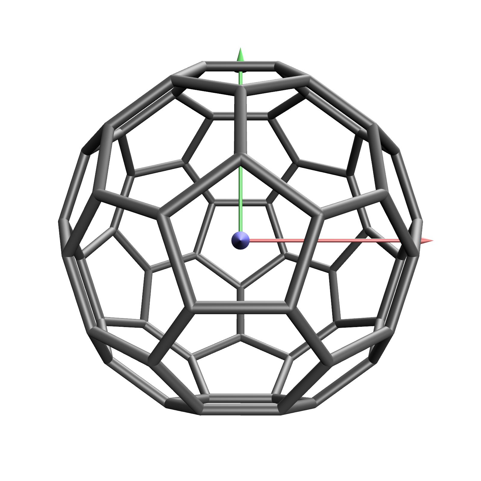
Figure 1: Axis orientation of C60. Red, green and blue arrows correspond to $x$, $y$ and $z$ directions respectively

Analysis of the spectroscopic data[4, 5] indicates that the PES is dominated by the distance of the encapsulated He atom from the centre of the cage. This motivates the partitioning of this PES as a two-dimensional ($r_{\ce{He}}$, $R_{\ce{C60}}$) radial surface to which four-dimensional ($r_{\ce{He}}$, $\theta$, $\phi$, $R_{\ce{C60}}$) corrections are added. These corrections are on the order 1cm^-1 , and add some fluctuations to an otherwise smooth, polynomial radial surface.

This form of PES necessitates the learning of two separate but linked GPs. Initially, the two-dimensional radial surface is trained on the majority of the data. The four-dimensional corrections are then trained the remaining input data, but with $y_{4D}=y_{2D}-\mu_{2D}$. That is to say, its outputs are the difference between the learned radial surface and electronic structure data. Finally, before training the four-dimensional surface, the input coordinates are symmetrised. This is accomplished by applying the $I_{h}$ symmetry operations $C_{5}^{n}$ for $n\in[0,1,2,3,4]$ using the axis aligned along the $z$ direction, and also the centre of inversion $i$, producing nine extra equivalent geometries with identical energies.

The quality of the PES is determined by the choice of kernel and distance metric used in the GP. For the two-dimensional radial surface, an anisotropic Matérn covariance function[81] with $\nu=2.5$ using the standard Euclidean distance added to a white noise function was chosen. For the four-dimensional surface, a more considered choice is required as the angular and radial components use different types of coordinates, units and possibly even distance metrics. Consequently, this kernel is split into the sum of a white noise function and a product of a radial and angular functions

$$K_{2D}(\mathbf{r},\mathbf{r}^{\prime}) =\sigma^{2}_{2D}k(\mathbf{r},\mathbf{r}^{\prime})+\text{Noise}$$ (7)

$$K_{4D}(\mathbf{R},\mathbf{R}^{\prime}) =\sigma^{2}_{4D}k_{r}(\mathbf{r},\mathbf{r}^{\prime})k_{a}(\bm{\Omega},\bm{\Omega}^{\prime})+\text{Noise}.$$ (8)

where $\mathbf{r}$ refers to the radial coordinates ($r_{\ce{He}}$, $R_{\ce{C60}}$), $\bm{\Omega}$ refers to the angular coordinates ($\theta$, $\phi$) and $\mathbf{R}:=(\mathbf{r},\bm{\Omega})$. The product of $k_{r}$ and $k_{a}$ is chosen as it treats both coordinate types on equal footing. An alternative choice of summed kernel here would treat the similarity as similar to the radii or the angles which would introduce artificial correlation with data.

While $k_{r}=k$ is a possible choice, a more nuanced approach is required for $k_{a}$. This is due to the use of spherical polar coordinates, and how this affects the choice of metric. As the angular coordinates (without loss of generality) lie on the surface of a unit sphere this provokes the choice of two metrics: chordal, which is the simple straight line distance; or great-circle, which is the geodesic on the sphere. This is calculated as

$$d_{\text{Great-Circle}}(\bm{\Omega},\bm{\Omega^{\prime}})=2\arcsin\left(\left[\sin^{2}(\frac{(\frac{\pi}{2}-\theta)-(\frac{\pi}{2}-\theta^{\prime})}{2})\right.\right.$$

$$+\left.\left.\cos(\frac{\pi}{2}-\theta)\cos(\frac{\pi}{2}-\theta^{\prime})\sin^{2}(\frac{\phi-\phi^{\prime}}{2})\right]^{0.5}\right)$$ (9)

$$d_{\text{Chordal}}=2\sin\left(\frac{d_{\text{Great-Circle}}}{2}\right)$$ (10)

where the spherical polar coordinates have been converted to longitude and latitude. This is easily converted to the chordal distance using the relationship given in Eq (10). If using the chordal metric, as this is analogous to the Euclidean distance of Cartesian coordinates, the usual choices of kernels are possible. However, should the great-circle distance be preferred, this is not the case as a positive-definite covariance matrix is not guaranteed. This is resolved by using compactly supported covariance functions[82, 83], examples of which are given in Table 1. These functions can also use the chordal distance, but as the geodesic does not distort these distances, that should be the preferred metric where possible. Due to the high symmetry of the endofullerene, this also motivates the use of a kernel that can emulate the radial and angular patterns within the input data, which is better achieved through the kernels listed in Table 1.

Kernel	Function	Geodesic Parameters
Matérn	$\frac{2^{1-\nu}}{\Gamma(\nu)}\left(\sqrt{2\nu}\frac{d}{l}\right)^{\nu}K_{\nu}\left(\sqrt{2\nu}\frac{d}{l}\right)$	$l>0;\,\nu\in(0,\frac{1}{2}]$
Wendland-C2	$\left(1+\tau\frac{d}{s}\right)\left(1-\frac{d}{s}\right)^{\tau}_{+}$	$s\in(0,\pi],\,\tau\geq 4$
Wendland-C4	$\left(1+\tau\frac{d}{s}+\frac{\tau^{2}-1}{3}\frac{d^{2}}{s^{2}}\right)\left(1-\frac{d}{s}\right)^{\tau}_{+}$	$s\in(0,\pi],\,\tau\geq 6$

Table 1: Kernels which give a positive-definite covariance matrix when using the spherical geodesic distance for $d$. In the Matérn, $\nu,l$ refer to the smoothness and length-scale. In the Wendland kernels, $\tau,s$ play analogous roles although $s$ is a support parameter and may not be optimisable. The subscript + is shorthand for max(f(x),0). If using the chordal metric, some parameter restrictions are lifted.

As we require the PES to be twice-differentiable, given the restriction on $\nu$ in Table 1 this removes the Matérn as a possibility. The Wendland kernels are dependent on two parameters: $\tau$, a smoothness parameter which is analogous to $\nu$ in the Matérn; and $s$ which appears to be an optimisable lengthscale but is actually a support parameter. To ensure differentiability of the Wendland kernel, we require $s\geq\text{max}(d)$ which is $\pi$ and 2, for the great-circle and chordal distances respectively. While in the latter case this could be an optimised hyperparameter, in both cases we choose to fix $s=\text{max}(d)$.

II.3 Diagonalising the Translational Hamiltonian

II.3.1 Full 4D Problem

The Hamiltonian for He@C60 including all degrees of freedom of the endohedral atom and the cage breathing in atomic units is given by

$$\hat{H}=\underbrace{-\frac{1}{2m}\nabla^{2}_{\mathbf{r}_{\ce{He}}}-\frac{1}{2M}\nabla^{2}_{R_{\ce{C60}}}+\frac{1}{2}k_{\ce{He}}r^{2}+\frac{1}{2}k_{\ce{C60}}R_{\ce{C60}}^{2}}_{\hat{H}^{0}}+\Delta V(\mathbf{R})$$ (11)

where $m$ is the reduced mass of the He–C60 “two-particle” system, $M$ is the mass of the C60 cage, $(r,\theta,\phi)$ refer to the endohedral coordinates of the He in spherical polars: distance from origin, polar and azimuthal angles respectively; and $R$ is the C60 cage radius. The harmonic contributions of the He translation and C60 cage breathing have been explicitly included as this enables the use of the following simple coordinate transformations

$$q_{\ce{He}} =r^{2}\sqrt{k_{\ce{He}}m}$$ (12)

$$q_{\ce{C60}} =(R_{\ce{C60}}-R_{\text{eq}})\sqrt{\sqrt{k_{\ce{C60}}M}}.$$ (13)

where $R_{\text{eq}}$ is the equilibrium C60 cage radius. By scaling both the He and C60 cage breathing to the natural length scales of the oscillators, and centring them at $q_{i}=0$, this allows for the basis set to be constructed from a three-dimensional harmonic oscillator (3D HO) for the He translation and a one-dimensional harmonic oscillator (1D HO) for the C60 cage breathing mode. Overall, the basis set is then written as

$$\ket{klmb}=\ket{kl}\ket{lm}\ket{b}=N_{klmb}L_{k}^{l+\frac{1}{2}}(q_{\ce{He}})Y_{lm}(\theta,\phi)H_{b}(q_{\ce{C60}})$$ (14)

where $N_{klmb}$ is the appropriate normalisation constant. Working in the finite basis representation (FBR), the $\hat{H}^{0}$ matrix is diagonal and depends only on the quantum numbers and frequencies of the two different oscillators. The potential energy matrix is a bit more cumbersome to work with. Traditionally this problem is solved using discrete variable representation (DVR) techniques[84, 85, 86], which require both the selection of basis set and quadrature points where this matrix would be diagonal, and the quadrature grid would normally be constructed as a direct product of smaller sub-dimensional grids.

However, as the angular momentum quantum number $l$ is shared between the radial and angular functions, a direct product grid is not possible. Nonetheless it is still possible to leverage advantages from using the DVR in this scenario. As this basis set is orthonormal, there exists an orthogonal transformation between the FBR and DVR. [84] This transformation from the DVR to the FBR corresponds to effectively evaluating the potential matrix elements using Gaussian quadrature.

An appropriate choice of values for $k_{\ce{He}}$ and $k_{\ce{C60}}$ in Equations (12) and (13) will correspond to the equivalent Gaussian quadrature points. There can be multiple choices for this: the traditional method, where an interval for each coordinate is chosen such that the potential doesn’t exceed a cutoff values, or a Potential-Optimised DVR[86] scheme where the shape and curvature of the potential dictates this scaling.

For the $q_{\ce{He}}$ coordinate, the atom is restricted to explore a sphere within the cage with $r_{\ce{He}}\in[0,1.5$Å], as even at the equilibrium cage radius beyond this interval the potential is greater than 5000cm^-1 . On the other hand, $q_{\ce{C60}}$ is scaled using the natural known frequency of the cage breathing mode of 500cm^-1 .

II.3.2 Comparison to 1D

After imposing spherical symmetry and fixing the cage radius, the simple 1D translational eigenstates can be calculated from the Hamiltonian[4, 5, 14]

$$\hat{H}=-\frac{1}{2m}\nabla^{2}_{\mathbf{r}_{\ce{He}}}+\frac{1}{2}kr^{2}+\Delta V(r).$$ (15)

A simple sixth degree polynomial for $V(r)$ has been fitted[4, 5], and by using the $\ket{kl}$ basis set as defined in Equation (14) but with $k$ chosen from a PODVR perspective, the one-dimensional eigenstates can be derived. Anharmonicity lifts the degeneracy of states with the same principal quantum number[4, 5] $n=2k+l$, but the lack of angular dependence in this potential implies no coupling of states with differing values of $l$ and maintains their $(2l+1)$-fold degeneracy. Under $I_{h}$, states with $l\geq 3$ are expected to have this degeneracy lifted but this is not observable with the purely one-dimensional radial potential.

The simplest comparison of the one-dimensional and four-dimensional problems is through the energy gaps between eigenstates as these are what can be measured spectroscopically. The importance of angular dependence in the potential can be determined by how strongly the $(2l+1)$-fold degeneracy of the spherically symmetric states is lifted.

Not only can the energies of the states be compared, but also the wavefunctions by considering their overlaps

$$\braket{\Phi}{\Psi} =\sum_{KLMB}\sum_{klmb}c_{KLMB}c_{klmb}\braket{KLMB}{klmb}$$

$$=\sum_{KLMB}\sum_{klmb}c_{KLMB}c_{klmb}\braket{KL}{kl}\braket{LM}{lm}\braket{B}{b}$$

$$=\sum_{KLMB}\sum_{klmb}c_{KLMB}c_{klmb}\braket{KL}{kl}\delta_{Ll}\delta_{Mm}\braket{B}{b}$$

$$=\sum_{KBklmb}c_{KlmB}c_{klmb}\braket{Kl}{kl}\braket{B}{b}.$$ (16)

While this is the general case for the overlap of two four-dimensional eigenstates, if $\bra{\Phi}$ is the one-dimensional reference, the $\bra{LM}\bra{B}$ functions have to be pre-selected. If they are chosen to be pure basis states, the sum over those indices collapses. The expected orthonormality of the integrals $\braket{Kl}{kl}$ and $\braket{B}{b}$ is not necessarily recovered due to the different scalings and centres of expansion, and they must be evaluated.

Instead of using the overlap which measures the similarity of the wavefunctions, an equivalent notion of how far apart the states are can be considered. The Hellinger distance [87], which is given by

$$H(\Phi,\Psi)=\sqrt{1-|\braket{\Phi}{\Psi}|}$$ (17)

can be used as an alternative. This requires both wavefunctions to be renormalised along the same measure guaranteeing $0\leq H\leq 1$ with equality holding if the states are completely identical or orthogonal respectively.

III Results

III.1 Potential Energy Surface

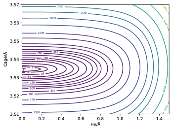
(a) MP2 Radial

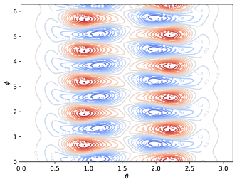
(b) MP2 Angular

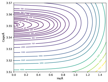
(c) RPA@PBE Radial

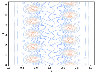
(d) RPA@PBE Angular

Figure 2: Two dimensional (a) MP2 radial, (b) MP2 angular, (c) RPA@PBE radial, and (d) RPA@PBE angular slices of the PES. Radial slices are taken at $(\theta,\phi)=(0,0)$, the energy zero set to the minimum of the slice and contours at [1, 5, 10, 25, 50, 75, 100, 150, 200, 250, 300, 400, 500, 750, 1000, 1500, 2000, 2500, 3000, 4000, 5000, 6000, 7000]cm^-1 . Angular slices are taken at $(r_{\ce{He}},R_{\ce{C60}})=(0.3066,3.54181)$, the energy zero at the origin and contours are every 0.5cm^-1 in the interval [-5, 5]cm^-1 .

For the two-dimensional radial kernel, $k$ defined in Eq (7), was chosen to take the form of an anisotropic Matérn covariance function with $\nu=2.5$. For the four-dimensional corrections with kernel of the form given in Eq (8), $k_{r}$ took the same form as $k$, whereas for $k_{a}$ we choose to use the Wendland-C4 covariance function shown in Table 1, with $\tau=6$ and the great-circle metric defined in Eq (9) enforcing $s=\pi$. Both kernels required the optimisation of four hyperparameters namely: amplitude, $r_{\ce{He}}$ and $R_{\ce{C60}}$ length-scales and the noise. Further details for training the GPs to generate the PESs are outlined within the supplementary information, Section SI 2.

Adding the predictions of these kernels together gives rise to the two-dimensional radial and angular slices of the four-dimensional PES seen in Fig 2. As the PES is defined up to an arbitrary energy shift, we choose the energy zero to be the energy minimum in the radial slice which is taken at $(\theta,\phi)=(0,0)$ and in the angular slice to be the value at the origin, with the radii frozen at $(r_{\ce{He}},\,R_{\ce{C60}})$ = (0.30066Å, 3.54181Å).

The shape of the radial slices is remarkably smooth along both radial coordinates. This indicates the radial surface can be well described by a polynomial oscillator. The $r_{\ce{He}}$ coordinate shows a considerable amount of anharmonicity as previously observed.[4, 5] The $R_{\ce{C60}}$ coordinate on the other hand shows very little anharmonicity. As the elliptical contours are almost perfectly aligned along these axes, this suggests there is unlikely to be any observable coupling between the He translational and C60 cage breathing modes.

These features are shared in both the MP2 and RPA@PBE radial surfaces, alongside the equilibrium He position being at the origin. This is expected given the $I_{h}$ symmetry of the system. However there is one stark difference being the equilibrium cage radius. MP2 predicts this to be at $R_{\ce{C60}}$ = 3.536Å  whereas the RPA@PBE predicts it to be at $R_{\ce{C60}}$ = 3.551Å. This difference of approximately 0.04% signifies the relevance of this coordinate in the surface which was previously neglected.[4, 5] Fig 2 also highlights the importance of the four-dimensional nature of the surface. Picking any particular one-dimensional slice through an ab initio PES with fixed $(\theta,\phi,R_{\ce{C60}})$ will lead to different translational energies.

Turning to the angular slices the contours are taken every 0.5cm^-1 in the interval [$-5$cm^-1 , $5$cm^-1 ]. There is a great similarity between the positions of the positive four-dimensional corrections given in red, and the negative shown in blue. Both the MP2 and RPA@PBE surfaces have a periodic $\frac{2\pi}{5}$ symmetry along the $\phi$ direction as necessitated by the symmetrisation of the data with the $C_{5}$ rotation axis. They also exhibit the symmetry of mirroring along $\theta=\frac{\pi}{2}$ and swapping the $\phi=(0,\pi)$ and $\phi=(\pi,2\pi)$ regions due to the inversion symmetry introduced into the training data.

However, the numerical values of the corrections are subtly different between the MP2 and RPA@PBE. The MP2 corrections span the full corrections range, whereas the RPA@PBE, with its much lighter contours only spans the range [$-2.5$cm^-1 , $2$cm^-1 ]. The sensitivity of these four-dimensional corrections is further illustrated in the SCS-MP2 and SOS-MP2 PES slices, which are given in the supplementary information Section SI 2. While these corrections are on the order of single digit wavenumbers, this weak angular dependence not being completely flat will lift the $(2l+1)$-fold degeneracy of the states in the traditional 3D HO. This is alongside the breaking of principal quantum number $n=2k+l$ degeneracy due to the radial anharmonicity.

(a) Radial lower bounds

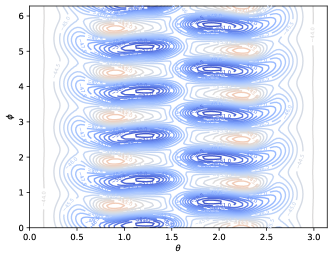
(b) Angular lower bounds

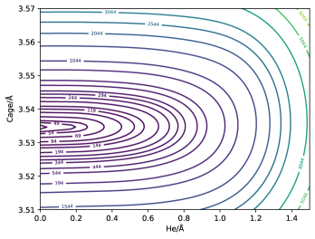
(c) Radial upper bounds

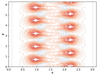
(d) Angular upper bounds

Figure 3: 95% confidence interval on the value of the four-dimensional corrections to a fixed two-dimensional radial MP2 PES: (a) radial lower bound, (b) angular lower bound, (c) radial upper bound, and (d) angular upper bound. The radial and angular slices are at the same fixed coordinates as in Fig 2. Radial contours have their values shifted by -44cm^-1 in the lower bound, and +44cm^-1 in the upper bound. Angular contours are at every 0.5cm^-1 relative to the value at the origin being -43.5cm^-1 in the lower bound and +43.5cm^-1 in the upper bound.

The choice of angular kernel and metric was made by comparing the 95% confidence interval on the surface prediction, whose lower and upper bound two-dimensional slices are shown in Fig 3. The radial slices are taken at the same fixed angular coordinates and vice versa as in Fig 2. These confidence intervals are calculated only from the error in the prediction of the four-dimensional corrections. This is equivalent to “pre-selecting” a two-dimensional radial surface and asking what is the possible range of values of the four-dimensional corrections. If the GPs are independent, the total error in each prediction would be given by $\sqrt{\Sigma_{2D}^{2}+\Sigma_{4D}^{2}}$. However, in this particular form of PES, this is likely to be an upper bound to the true confidence interval, as the two-dimensional GP and four-dimensional GP would have a negative cross-covariance. This is because as the two-dimensional surface becomes more accurate, the four-dimensional surface becomes more flat.

The radial lower and upper bound surfaces for MP2 look almost identical to the mean surface prediction. The contours are centred at the minimum of the surface, but taken at 44cm^-1 lower and higher than the values in Fig 2. While this confidence interval of 88cm^-1 may seem quite large, as the PES is only defined up to an arbitrary energy zero, it can be linearly shifted without affecting the subsequent calculations. This is an indication of the kernel constraining the behaviour of the GP, strongly enforcing the overall shape of the PES. As further calculations using the PES are agnostic of the energy zero, the mapping $E=E_{2D}+E_{4D}\rightarrow(E_{2D}+\delta E_{2D})+(E_{4D}+\delta E_{4D})$ will maintain the subsequent properties derived from the PES. Therefore this wide confidence interval is not diagnostic of a poor PES.

The angular lower and upper bounds however, show a more involved behaviour. With the centre of the contours at the origin, at -43.5cm^-1 and +43.5cm^-1 respectively, the confidence interval still maintains the same $\frac{2\pi}{5}$ periodic and inversion symmetry. While the range of the upper and lower bound surfaces are still approximately 10cm^-1 , analogous to the mean prediction, there is a dominance towards the extremes of each bound. That is to say, the lower bound surface shows tendency to skew towards a more negative correction and vice-versa. This implies the confidence interval is somewhat spiky, with a width in places of over 100cm^-1 . Once again, as the PES is only defined up to an arbitrary energy zero, the shape of these errors is of more importance. The consequence of the exact shape and size of the PES and confidence interval will be observed in the degree of splitting of the $(2l+1)$-fold degenerate energy levels and the size of error bars on the translational eigenstates seen in Fig 4.

This choice of kernel and metric had the tightest confidence interval of all possible options indicated in Table 1. The ranges of the other options of kernel and metric for MP2 are given in the supplementary information Section SI 2. While the shape of these confidence intervals and PES is more important than its width, it is still prudent to try to tighten them. The errors could arise due to a combination of factors including the choice of metric which dictates the value of the support parameter $s$ defined in Table 1, or even because $\tau$ is fixed. They may also be a consequence of the tight hyperparameter bounds on the four-dimensional kernel imposed by chemical intuition. However, widening them could lead to a very flat surface prediction by the GP. On the other hand, introducing more training data could lead to overfitting of the surface. Noticing the Wendland-C4 being an improvement on the Wendland-C2 opens a possible systematic route to better choices for $k_{a}$. This could be achieved by generating higher degree Wendland functions[88] and using them with the great-circle metric as the angular kernel.

III.2 Translational Eigenstates

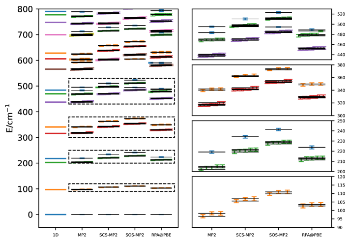
Figure 4: Four-dimensional translational energies of He@C60 for MP2, SCS-MP2, SOS-MP2, and RPA@PBE PESs alongside the one-dimensional experimental derived counterparts. One-dimensional energies are coloured by angular momentum quantum number $l$ in increasing order: blue, orange, green, red, purple, brown, pink and grey. Error bars on the electronic structure methods are also coloured according to the near degeneracy of states.

The nuclear Hamiltonian in Eq (11) was diagonalised using basis functions of the form defined in Eq (14), with 10 translational $\ket{kl}$ functions for each $l$, spherical harmonics $\ket{lm}$ with $l\leq 7$, and 4 cage breathing $\ket{b}$ functions. This gave an overall basis set size of 2560 functions. The 100 lowest lying eigenstates were converged to within 0.5cm^-1 , with the majority of states converging to within 0.02cm^-1 .

These eigenstates are plotted, with the ground state energy set to be the energy zero, in Fig 4, alongside energies from the spherically symmetric one-dimensional potential. As these were generated from a potential fitted to the spectroscopic data, they are equivalent for comparison. These one-dimensional energies are colour coded by their angular momentum quantum number, $l$. Due to the spherical symmetry, these states are $(2l+1)$-fold degenerate, but the principal quantum number of the 3D HO $n=2k+l$ which usually gives $\lceil\frac{n}{2}\rceil$-fold degeneracy (ignoring the $l$ degeneracy effect), is lifted. This is due to the anharmonic nature of the potential along $r_{\ce{He}}$, which is also seen in Fig 2.

This anharmonicity is recovered in all four electronic structure methods: MP2, SCS-MP2, SOS-MP2 and RPA@PBE. Looking at the energies of these translational eigenstates, it is noticeable that they are consistently substantially overestimated by the two semi-empirical methods SCS-MP2 and SOS-MP2. The fundamental transition differs by approximately 10cm^-1   to the spectroscopic data, with higher energy states having sequentially worse agreement. The two ab initio methods on the other hand perform considerably better, with MP2 predicting a fundamental frequency of $96.58\pm 0.99$cm^-1 which has very good agreement to the spectroscopic value of 96.7cm^-1 .[4, 5] The RPA@PBE consistently overestimates these energies by approximately 6cm^-1 . The possible causes of these discrepancies to the one-dimensional data are described in Section II.1: the MP2 lacking screening effects, and the RPA@PBE not including exchange effects. While a priori it is not obvious which is the more significant effect, the comparison to the spectroscopic data indicates that the MP2 outperforms the RPA@PBE. However, it should be noted that, due to the neglect of exchange effects between particle-hole pairs, RPA@PBE exhibits significantly higher efficiency compared to the MP2 method. To illustrate, a single MP2 calculation using a quadruple-zeta basis set takes approximately 325 min, whereas the corresponding RPA@PBE calculation requires about 34 min. This makes the MP2 method roughly ten times as computationally expensive as the RPA calculation. Therefore, although the energies predicted by RPA@PBE do not converge to spectroscopic accuracy, the significantly higher computational efficiency of this electronic structure method suggests that it should not be discarded as a viable choice for these systems.

We also observe a lifting of the of the $(2l+1)$-fold degeneracy in all four electronic structure methods, but to varying degrees, indicating different levels of importance on angular dependence within the PES. All three MP2 methods predict a $p$-state splitting of over 1cm^-1 and a $d$-state splitting ranging to over 3cm^-1 whereas the RPA@PBE predicts these splittings to be 0.85cm^-1 and 2cm^-1 respectively. However, considering the $I_{h}$ character table, all three $p$ states and five $d$ states are expected to be degenerate. This fictitious splitting arises due to the symmetrisation of the data using only a single $C_{5}$ rotation axis and the centre of inversion $i$. This only generates a subgroup symmetry of $I_{h}$, namely $D_{5d}$, where the $p$ and $d$ state splitting is expected. Fully symmetrising the training data is a non-trivial task due to the orientation of the C60 cage shown in Fig 1 and position of the remaining symmetry elements. This would also be counter-productive to the problem as it would lead to strong overfitting in the PES, making it very spiky at the location of the training data.

For states with $l\geq 3$, namely $f$ states and higher, there is a real splitting of these states as expected under $I_{h}$ symmetry, of 4cm^-1 in the MP2 and 2.5cm^-1 in the RPA@PBE. The smaller splitting is expected in the RPA@PBE, as the range of the angular PES slice in Fig 2 is smaller than the equivalent MP2 range. This real splitting indicates the importance of catering for the angular dependence in the PES, as this allows for states with differing $l$ to couple and mix, which is not possible with a purely symmetric potential. The lifting of this degeneracy may be masked within an experimental spectrum into the linewidth of the corresponding transition.

For the states with energies under 500cm^-1 , there is a one-to-one mapping of the one-dimensional energy levels, to the ones of each electronic structure method. However, around 500cm^-1 , an extra state appears in the electronic structure diagonalisation. This is due to the excitation of a quantum in the cage breathing mode but remaining in the ground translational state. In the three MP2 methods, the fundamental cage breathing frequency is 495cm^-1 , but 490cm^-1 in the RPA@PBE. Looking at the top right insert in Fig 4, this extra state is obvious in the MP2, SOS-MP2 and RPA@PBE, but seems to be missing in the SCS-MP2. It is necessarily still present, but has been mixed into the cluster of the first set of excited $d$ states.

Going upwards in energy, all the states with energy $<500$cm^-1 will be repeated again, with an excitation in the breathing mode. These will be combined with the higher pure translational excitations which leads to a cluttered energy level diagram and increases the difficulty in matching the one-dimensional energies to the electronic structure analogues. There seems to be no discernible coupling of the breathing mode to the translational mode, as the combination modes occur at the sum of energies of exciting each mode separately. This is expected given the form of radial slices in the PES in Fig 2, with the contours aligning almost perfectly along the radial axes.

An advantage of using GPR for PES interpolation, is the ability to generate the covariance matrix as defined in Eq (5), alongside its mean prediction given by Eq (4). We construct the overall covariance matrix as $\bm{\Sigma}=\bm{\Sigma}_{2D,2D}+\bm{\Sigma}_{4D,4D}$, which is exact assuming independence between each GP. However, as mentioned in Section III.1, there is likely to be a negative cross covariance between these processes denoted by $\bm{\Sigma}_{2D,4D}$, implying the error bars shown in Fig 4 are upper bounds to the “true” errors. These error bars were calculated by generating 100 samples of the PES from the appropriate multivariate Gaussian distribution which in turn generates 100 different nuclear Hamiltonian matrices. The eigenvalues of these matrices were averaged, generating its mean and standard deviation. These error bars are also colour coded by near degeneracy of the states. For states with energies below 500cm^-1 , this corresponds identically to the angular momentum quantum number, $l$, with the spectroscopic reference. Above this, however, this may not be the case due to the muddling of states involving an excitation in the breathing mode.

Looking at the four zoomed-in inserts in Fig 4, it is noticeable how small these error bars are, usually less than $\pm 2$cm^-1 . Despite the wide looking 95% confidence interval seen in Fig 3, this ends up being a relatively small error bar in the translational energy, which may be interpreted in relation to a linewidth in an experimental spectrum. The minute size of these error bars once again demonstrates the dominance of the two-dimensional radial PES, compared to the four-dimensional corrections. The error bars on the MP2 translational energies are smaller than those of the RPA@PBE, despite the angular corrections being larger in magnitude. This implies the confidence interval on the MP2 surface is tighter than the respective one for RPA@PBE.

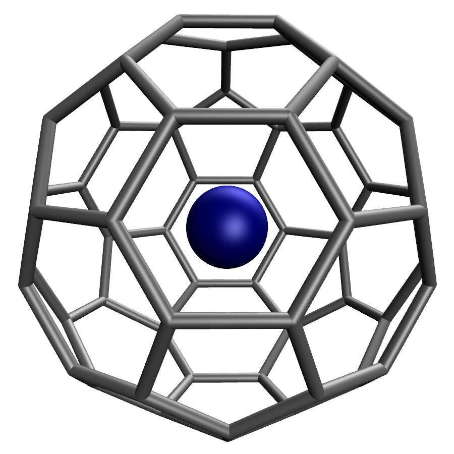
(a) $s$

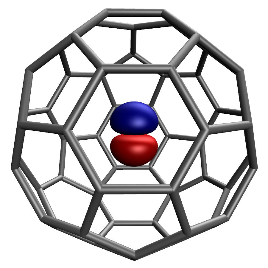
(b) $p$

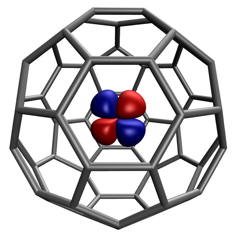
(c) $d$

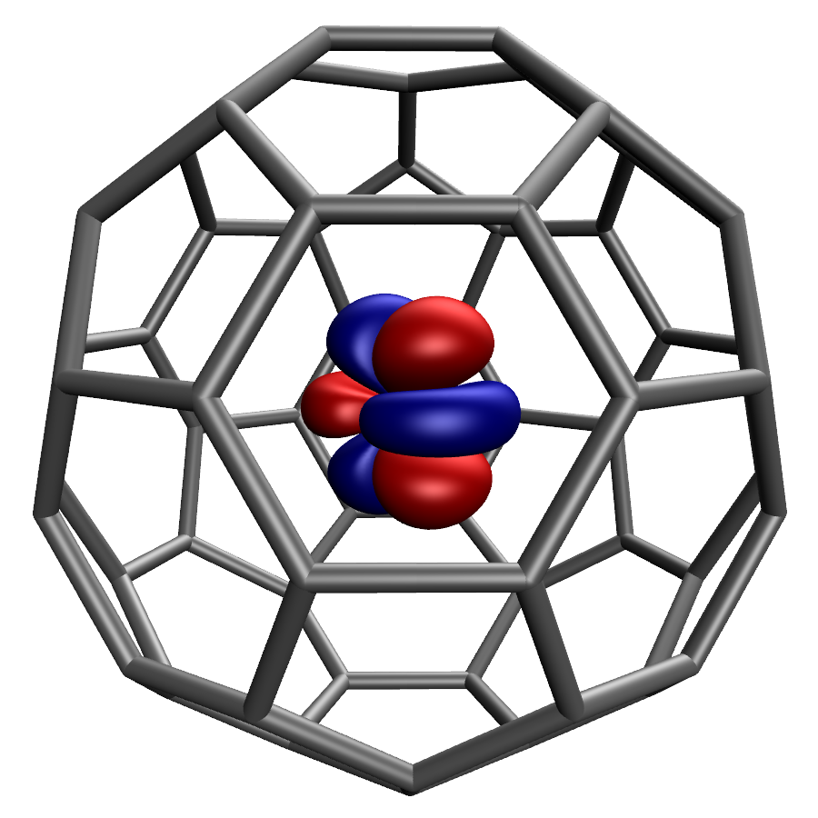
(d) $f$

Figure 5: MP2 isosurfaces of (one of) the lowest lying set of (a) $s$, (b) $p$, (c) $d$, and (d) $f$ nuclear orbitals. The C60 cage has been rotated relative to Fig 1, with the $z$ direction pointing directly upwards, and $xy$ plane rotated to centre down a $C_{3}$ axis. The isosurfaces are taken at 0.5% of the maximum amplitude of each wavefunction.

Electronic Structure Method	Overlap	Hellinger Distance
MP2	0.99644	0.08424
SCS-MP2	0.99335	0.11508
SOS-MP2	0.99146	0.13081
RPA@PBE	0.99440	0.10560

Table 2: Overlap and Hellinger distance of the ground state wavefunction for MP2, SCS-MP2, SOS-MP2 and RPA@PBE with the experimentally derived one-dimensional ground state.

$\bra{\downarrow}$, $\ket{\rightarrow}$	MP2	SCS-MP2	SOS-MP2	RPA@PBE
MP2	-	0.04055	0.05880	0.02617
SCS-MP2	0.04055	-	0.01831	0.02357
SOS-MP2	0.05880	0.01831	-	0.03987
RPA@PBE	0.02617	0.02357	0.03987	-

Table 3: Hellinger distances of the ground state between all four electronic structure methods. Diagonal elements, by definition, are necessarily zero.

The energies are not the only information obtained from the diagonalisation procedure; the eigenvectors corresponding to the wavefunctions are also obtained. These nuclear wavefunctions (orbitals) have strikingly regular patterns as seen in Fig 5, which allows for simple assignment of both translational and total angular momentum quantum numbers $k$ and $l$ respectively. These eigenfunctions are usually dominated by a single 3D HO wavefunction. With the reorientation of the cage to have the $z$ direction pointing upwards, it is interesting to see the rotation along this axis of the $f$ orbital in relation to the $d$ orbital. It turns out neither are perfectly aligned along either the $x$ or $y$ directions, suggesting that this particular set of $x$ and $y$ axes is not best suited to the Cartesian representation of these orbitals. The isosurfaces, taken at 0.5% of the maximum amplitude of each wavefunction are constrained within a sphere of radius 1.5Å  which is less than 50% the value of the C60 cage radius. This implies that while the He is encapsulated within the C60 cage, it does not explore any region close to the C atoms.

Instead of using the energies as the discriminator for the validity of electronic structure method, the wavefunction can be used instead. This is achieved by considering the overlap, or by calculating the Hellinger distance, as defined in Eqns (16) and (17) respectively between the one-dimensional reference state and four-dimensional eigenfunction. Considering just the ground state, we take the reference $\bra{LM}\bra{B}$ states to be the pure basis state $\bra{00}\bra{0}$, reducing the summation over $lmb$ quantum numbers to a single term. Due to the different equilibrium cage radii predicted by each electronic structure method, the centre of expansion of these breathing 1D HO functions is different. For each electronic structure method, we enforce the reference 1D breathing state to be centred in the same position. This has the intended effect of the Hellinger distance (and overlap) to be purely due to the difference in the translational portion of the eigenfunction. These overlaps and distances are given in Table 2. While all these methods have over 99% overlap with the reference one-dimensional ground state, the distinction in their quality is more apparent in their Hellinger distances. In line with the energy matches, the ab initio MP2 and RPA@PBE perform best, with the semi-empirical SCS-MP2 and SOS-MP2 lagging behind. This seems to indicate that either the energy, or the Hellinger distance could be used interchangeably as the validator of the electronic structure method.

Despite the spectroscopic accuracy in the energy prediction of the MP2, the Hellinger distance still seems fairly large. This could be due to the extra angular dependence in the potential, allowing the mixing of states with differing angular momentum quantum number $l$ to couple, which is not possible in a purely spherically symmetric potential. This casts doubt on the correctness of the one-dimensional potential as while this fits the spectroscopic data, might not correspond to any particular one-dimensional slice of the four-dimensional PES.

Not only can the wavefunctions calculated from the electronic structure methods be compared to just the one-dimensional reference, they can also be compared to each other. The Hellinger distances of the ground state between electronic structure methods is given in Table 3. Once again, for the $\braket{B}{b}$ integral, despite the differing centres of expansion, we enforce this to be $\delta_{Bb}$ to isolate just the translational states. Due to the high frequency of the cage breathing mode, if these integrals were left in, the distances would all be over 0.70. Considering just the translational states, we find that all these methods are closer to each other than they are to the one-dimensional reference. This is possibly due to the angular dependence, with the sum over $lmb$ in Eq (17) not collapsing as both wavefunctions are four-dimensional. The SCS-MP2 and SOS-MP2 are most similar, closely followed by the MP2 and RPA@PBE, which follows suit from the energy level diagram in Fig 4.

IV Conclusion

In this work, we have investigated how the angular dependence of the potential energy surface and the cage breathing mode impact the translational eigenstates of the He@C60 endofullerene. For this investigation, we calculated complete basis set extrapolated four-dimensional potential energy surfaces, incorporating three He translational degrees of freedom and the C60 cage radius, using various electronic structure methods: MP2, SOS-MP2, SCS-MP2, and RPA@PBE. The rationale for utilising this array of methods is twofold: by comparing their results, we have gained not only confidence in our findings but also valuable insights into the performance of these methods where comparisons with reference data were feasible.

Due to the high computational cost of the electronic structure calculations, the full Potential Energy Surface (PES) required interpolation from this sparse training data which was performed using Gaussian Process Regression. The PES was partitioned into a two-dimensional radial surface, to which corrections were applied making it overall four-dimensional. This is a well motivated choice due to the lack of obvious angular splitting within the spectroscopic data. The expression of the PES using spherical polar coordinates motivated the form of kernels shown in Eqns (7) and (8), which required a nuanced choice of the angular kernel $k_{a}$ and its metric. We chose to use the Wendland-C4, as shown in Table 1 with the great-circle metric as defined in Eq (9) as this accurately reflected the symmetry within the endofullerene, and had the smallest 95% confidence interval as seen in Figs 2. and 3.

We generated the four-dimensional translational eigenstates of He@C60 by diagonalising the nuclear Hamiltonian. By not enforcing spherical symmetry in the potential, and allowing states for different angular momenta to couple we find the $(2l+1)$-fold degeneracy of states to be lifted. The three MP2 type methods all predict very similar levels of splitting, whereas the RPA@PBE predicts smaller splittings. While some of this is artificial due to not exploiting the full $I_{h}$ symmetry of the system, we do observe a true splitting of $f$ states and higher of approximately 4cm^-1 . This suggests while the angular dependence is weak, it can still be observable in the broadening of these peaks in the spectra. On the other hand, we find very little influence on the cage breathing mode on these translational states.

Comparing the energies to the one-dimensional case, we find that the two ab initio methods: RPA@PBE and MP2 outperform the empirical methods SCS-MP2 and SOS-MP2. Comparing the energies as seen in Figure 4, MP2 has the best agreement with the one-dimensional case, achieving sub-wavenumber accuracy with the spectroscopic data.[4, 5] On the other hand, RPA@PBE exhibits a discrepancy of approximately 6cm^-1 compared to the experimental results; however, it proves significantly more efficient than MP2, surpassing it by almost an order of magnitude.

Furthermore, the wavefunctions of the ground state were compared to the one-dimensional case through their overlap and Hellinger distances in Tables 2 and 3. Once again we find that the MP2 and RPA@PBE eclipse the empirical SCS-MP2 and SOS-MP2. Considering the overall efficacy of these methods, and the trade-off between accuracy and computational cost we can recommend both MP2 and RPA@PBE as viable electronic structure methods for these systems.

Going forwards, a natural extension would be to apply these electronic structure calculations to larger endofullerenes, whether that be molecules within C60 such as H2@C60[6, 8, 9, 7] and H2O@C60[89, 90, 91, 92] which are popular in the literature or by considering larger fullerene cages such as Ne@C70.[93] An extra challenge for the latter system is to accurately describe the double well that is opened up by elongating the cage along the unique axis and reducing the symmetry to $D_{5h}$.[15]

While knowledge of the PES gave us access to the translational eigenstates, in order to accurately reproduce an experimental spectrum the knowledge of intensities of transitions is also required. This necessitates the calculation of a dipole moment surface (DMS), which could be generated and interpolated in an analogous way to the PES[11]. Knowledge of the DMS allows for the calculation of the transition dipole moment integrals which are fundamental in calculating the transition intensities.

Supplementary Information

See the supplementary information for more details on the electronic structure methods used, the training of the Gaussian Process and diagonalisation procedure. Extra results using different electronic structure methods, kernels and metrics are also provided.

Data Availability Statement

The data that support the findings of this study are openly available in Apollo - University of Cambridge Repository at.

References

- Murata et al. [2008] M. Murata, S. Maeda, Y. Morinaka, Y. Murata, and K. Komatsu, “Synthesis and Reaction of Fullerene C70 Encapsulating Two Molecules of H2,” J. Am. Chem. Soc. 130, 15800–15801 (2008).
- Bloodworth and Whitby [2022] S. Bloodworth and R. J. Whitby, “Synthesis of endohedral fullerenes by molecular surgery,” Commun Chem 5, 1–14 (2022).
- Bačić [2018] Z. Bačić, “Perspective: Accurate treatment of the quantum dynamics of light molecules inside fullerene cages: Translation-rotation states, spectroscopy, and symmetry breaking,” J. Chem. Phys. 149, 100901 (2018).
- Bacanu et al. [2021] G. R. Bacanu, T. Jafari, M. Aouane, J. Rantaharju, M. Walkey, G. Hoffman, A. Shugai, U. Nagel, M. Jiménez-Ruiz, A. J. Horsewill, S. Rols, T. Rõõm, R. J. Whitby, and M. H. Levitt, “Experimental determination of the interaction potential between a helium atom and the interior surface of a C60 fullerene molecule,” J. Chem. Phys. 155, 144302 (2021).
- Jafari et al. [2022] T. Jafari, G. R. Bacanu, A. Shugai, U. Nagel, M. Walkey, G. Hoffman, M. H. Levitt, R. J. Whitby, and T. Rõõm, “Terahertz spectroscopy of the helium endofullerene He@C60,” Phys. Chem. Chem. Phys. 24, 9943–9952 (2022).
- Xu et al. [2008a] M. Xu, F. Sebastianelli, Z. Bačić, R. Lawler, and N. J. Turro, “H2, HD, and D2 inside C60: Coupled translation-rotation eigenstates of the endohedral molecules from quantum five-dimensional calculations,” J. Chem. Phys. 129, 064313 (2008a).
- Xu et al. [2008b] M. Xu, F. Sebastianelli, Z. Bačić, R. Lawler, and N. J. Turro, “Quantum dynamics of coupled translational and rotational motions of H2 inside C60,” J. Chem. Phys. 128, 011101 (2008b).
- Xu et al. [2009] M. Xu, F. Sebastianelli, B. R. Gibbons, Z. Bačić, R. Lawler, and N. J. Turro, “Coupled translation-rotation eigenstates of H2 in C60 and C70 on the spectroscopically optimized interaction potential: Effects of cage anisotropy on the energy level structure and assignments,” J. Chem. Phys. 130, 224306 (2009).
- Xu et al. [2013] M. Xu, S. Ye, A. Powers, R. Lawler, N. J. Turro, and Z. Bačić, “Inelastic neutron scattering spectrum of H2@C60 and its temperature dependence decoded using rigorous quantum calculations and a new selection rule,” The Journal of Chemical Physics 139, 064309 (2013).
- Felker and Bačić [2016] P. M. Felker and Z. Bačić, “Communication: Quantum six-dimensional calculations of the coupled translation-rotation eigenstates of H 2 O@C 60,” J. Chem. Phys. 144, 201101 (2016).
- Kalugina and Roy [2017] Y. N. Kalugina and P.-N. Roy, “Potential energy and dipole moment surfaces for HF@C60: Prediction of spectral and electric response properties,” J. Chem. Phys. 147, 244303 (2017).
- Xu, Felker, and Bačić [2020] M. Xu, P. M. Felker, and Z. Bačić, “Light molecules inside the nanocavities of fullerenes and clathrate hydrates: Inelastic neutron scattering spectra and the unexpected selection rule from rigorous quantum simulations,” International Reviews in Physical Chemistry 39, 425–463 (2020).
- Felker and Bačić [2020] P. M. Felker and Z. Bačić, “Flexible water molecule in C 60 : Intramolecular vibrational frequencies and translation-rotation eigenstates from fully coupled nine-dimensional quantum calculations with small basis sets,” J. Chem. Phys. 152, 014108 (2020).
- Jafari et al. [2023] T. Jafari, A. Shugai, U. Nagel, G. R. Bacanu, M. Aouane, M. Jiménez-Ruiz, S. Rols, S. Bloodworth, M. Walkey, G. Hoffman, R. J. Whitby, M. H. Levitt, and T. Rõõm, “Ne, Ar, and Kr oscillators in the molecular cavity of fullerene C60,” The Journal of Chemical Physics 158, 234305 (2023).
- Panchagnula and Thom [2023] K. Panchagnula and A. J. W. Thom, “Exploring the parameter space of an endohedral atom in a cylindrical cavity,” The Journal of Chemical Physics 159, 164308 (2023).
- Noé et al. [2020] F. Noé, A. Tkatchenko, K.-R. Müller, and C. Clementi, “Machine Learning for Molecular Simulation,” Annu. Rev. Phys. Chem. 71, 361–390 (2020).
- Deringer et al. [2021] V. L. Deringer, A. P. Bartók, N. Bernstein, D. M. Wilkins, M. Ceriotti, and G. Csányi, “Gaussian Process Regression for Materials and Molecules,” Chem. Rev. 121, 10073–10141 (2021).
- Loeppky, Sacks, and Welch [2009] J. L. Loeppky, J. Sacks, and W. J. Welch, “Choosing the Sample Size of a Computer Experiment: A Practical Guide,” Technometrics 51, 366–376 (2009).
- Behler [2016] J. Behler, “Perspective: Machine learning potentials for atomistic simulations,” The Journal of Chemical Physics 145, 170901 (2016).
- Musil et al. [2021] F. Musil, A. Grisafi, A. P. Bartók, C. Ortner, G. Csányi, and M. Ceriotti, “Physics-Inspired Structural Representations for Molecules and Materials,” Chem. Rev. 121, 9759–9815 (2021).
- Dral et al. [2017] P. O. Dral, A. Owens, S. N. Yurchenko, and W. Thiel, “Structure-based sampling and self-correcting machine learning for accurate calculations of potential energy surfaces and vibrational levels,” The Journal of Chemical Physics 146, 244108 (2017).
- Westermayr et al. [2021] J. Westermayr, M. Gastegger, K. T. Schütt, and R. J. Maurer, “Perspective on integrating machine learning into computational chemistry and materials science,” The Journal of Chemical Physics 154, 230903 (2021).
- Westermayr and Marquetand [2021] J. Westermayr and P. Marquetand, “Machine Learning for Electronically Excited States of Molecules,” Chem. Rev. 121, 9873–9926 (2021).
- Collins [2002] M. A. Collins, “Molecular potential-energy surfaces for chemical reaction dynamics,” Theor Chem Acc 108, 313–324 (2002).
- Bartók et al. [2013] A. P. Bartók, M. J. Gillan, F. R. Manby, and G. Csányi, “Machine-learning approach for one- and two-body corrections to density functional theory: Applications to molecular and condensed water,” Phys. Rev. B 88, 054104 (2013).
- Albertani and Thom [2023a] F. E. A. Albertani and A. J. W. Thom, “Global descriptors of a water molecule for machine learning of potential energy surfaces,” (2023a), arxiv:2301.03853 [physics] .
- Albertani and Thom [2023b] F. E. A. Albertani and A. J. W. Thom, “Optimised Morse transform of a Gaussian process feature space,” (2023b), arxiv:2301.02172 [physics] .
- Teale et al. [2022] A. M. Teale, T. Helgaker, A. Savin, C. Adamo, B. Aradi, A. V. Arbuznikov, P. W. Ayers, E. J. Baerends, V. Barone, P. Calaminici, E. Cancès, E. A. Carter, P. K. Chattaraj, H. Chermette, I. Ciofini, T. D. Crawford, F. D. Proft, J. F. Dobson, C. Draxl, T. Frauenheim, E. Fromager, P. Fuentealba, L. Gagliardi, G. Galli, J. Gao, P. Geerlings, N. Gidopoulos, P. M. W. Gill, P. Gori-Giorgi, A. Görling, T. Gould, S. Grimme, O. Gritsenko, H. J. A. Jensen, E. R. Johnson, R. O. Jones, M. Kaupp, A. M. Köster, L. Kronik, A. I. Krylov, S. Kvaal, A. Laestadius, M. Levy, M. Lewin, S. Liu, P.-F. Loos, N. T. Maitra, F. Neese, J. P. Perdew, K. Pernal, P. Pernot, P. Piecuch, E. Rebolini, L. Reining, P. Romaniello, A. Ruzsinszky, D. R. Salahub, M. Scheffler, P. Schwerdtfeger, V. N. Staroverov, J. Sun, E. Tellgren, D. J. Tozer, S. B. Trickey, C. A. Ullrich, A. Vela, G. Vignale, T. A. Wesolowski, X. Xu, and W. Yang, “DFT exchange: Sharing perspectives on the workhorse of quantum chemistry and materials science,” Phys. Chem. Chem. Phys. 24, 28700–28781 (2022).
- Pérez-Jordá and Becke [1995] JoséM. Pérez-Jordá and A. D. Becke, “A density-functional study of van der Waals forces: Rare gas diatomics,” Chemical Physics Letters 233, 134–137 (1995).
- Grimme et al. [2016] S. Grimme, A. Hansen, J. G. Brandenburg, and C. Bannwarth, “Dispersion-Corrected Mean-Field Electronic Structure Methods,” Chem. Rev. 116, 5105–5154 (2016).
- Grimme [2004] S. Grimme, “Accurate description of van der Waals complexes by density functional theory including empirical corrections,” Journal of Computational Chemistry 25, 1463–1473 (2004).
- Antony and Grimme [2006] J. Antony and S. Grimme, “Density functional theory including dispersion corrections for intermolecular interactions in a large benchmark set of biologically relevant molecules,” Phys. Chem. Chem. Phys. 8, 5287–5293 (2006).
- Grimme [2006] S. Grimme, “Semiempirical GGA-type density functional constructed with a long-range dispersion correction,” Journal of Computational Chemistry 27, 1787–1799 (2006).
- Grimme et al. [2010] S. Grimme, J. Antony, S. Ehrlich, and H. Krieg, “A consistent and accurate ab initio parametrization of density functional dispersion correction (DFT-D) for the 94 elements H-Pu,” The Journal of Chemical Physics 132, 154104 (2010).
- Caldeweyher, Bannwarth, and Grimme [2017] E. Caldeweyher, C. Bannwarth, and S. Grimme, “Extension of the D3 dispersion coefficient model,” The Journal of Chemical Physics 147, 034112 (2017).
- Caldeweyher et al. [2019] E. Caldeweyher, S. Ehlert, A. Hansen, H. Neugebauer, S. Spicher, C. Bannwarth, and S. Grimme, “A generally applicable atomic-charge dependent London dispersion correction,” The Journal of Chemical Physics 150, 154122 (2019).
- Mardirossian and Head-Gordon [2017] N. Mardirossian and M. Head-Gordon, “Thirty years of density functional theory in computational chemistry: An overview and extensive assessment of 200 density functionals,” Molecular Physics 115, 2315–2372 (2017).
- Giner et al. [2018] E. Giner, B. Pradines, A. Ferté, R. Assaraf, A. Savin, and J. Toulouse, “Curing basis-set convergence of wave-function theory using density-functional theory: A systematically improvable approach,” The Journal of Chemical Physics 149, 194301 (2018).
- Kato [1957] T. Kato, “On the eigenfunctions of many-particle systems in quantum mechanics,” Communications on Pure and Applied Mathematics 10, 151–177 (1957).
- Fabiano and Della Sala [2012] E. Fabiano and F. Della Sala, “Accuracy of basis-set extrapolation schemes for DFT-RPA correlation energies in molecular calculations,” Theor Chem Acc 131, 1278 (2012).
- Pulay [1983] P. Pulay, “Localizability of dynamic electron correlation,” Chemical Physics Letters 100, 151–154 (1983).
- Häser [1993] M. Häser, “Møller-Plesset (MP2) perturbation theory for large molecules,” Theoret. Chim. Acta 87, 147–173 (1993).
- Maslen and Head-Gordon [1998] P. E. Maslen and M. Head-Gordon, “Non-iterative local second order Møller–Plesset theory,” Chemical Physics Letters 283, 102–108 (1998).
- Ayala and Scuseria [1999] P. Y. Ayala and G. E. Scuseria, “Linear scaling second-order Moller–Plesset theory in the atomic orbital basis for large molecular systems,” The Journal of Chemical Physics 110, 3660–3671 (1999).
- Schütz, Hetzer, and Werner [1999] M. Schütz, G. Hetzer, and H.-J. Werner, “Low-order scaling local electron correlation methods. I. Linear scaling local MP2,” The Journal of Chemical Physics 111, 5691–5705 (1999).
- Saebø and Pulay [2001] S. Saebø and P. Pulay, “A low-scaling method for second order Møller–Plesset calculations,” The Journal of Chemical Physics 115, 3975–3983 (2001).
- Werner, Manby, and Knowles [2003] H.-J. Werner, F. R. Manby, and P. J. Knowles, “Fast linear scaling second-order Møller-Plesset perturbation theory (MP2) using local and density fitting approximations,” The Journal of Chemical Physics 118, 8149–8160 (2003).
- Jung and Head-Gordon [2006] Y. Jung and M. Head-Gordon, “A fast correlated electronic structure method for computing interaction energies of large van der Waals complexes applied to the fullerene–porphyrin dimer,” Phys. Chem. Chem. Phys. 8, 2831–2840 (2006).
- Jung, Shao, and Head-Gordon [2007] Y. Jung, Y. Shao, and M. Head-Gordon, “Fast evaluation of scaled opposite spin second-order Møller–Plesset correlation energies using auxiliary basis expansions and exploiting sparsity,” Journal of Computational Chemistry 28, 1953–1964 (2007).
- Doser, Lambrecht, and Ochsenfeld [2008] B. Doser, D. S. Lambrecht, and C. Ochsenfeld, “Tighter multipole-based integral estimates and parallel implementation of linear-scaling AO–MP2 theory,” Phys. Chem. Chem. Phys. 10, 3335–3344 (2008).
- Doser et al. [2009] B. Doser, D. S. Lambrecht, J. Kussmann, and C. Ochsenfeld, “Linear-scaling atomic orbital-based second-order Møller–Plesset perturbation theory by rigorous integral screening criteria,” The Journal of Chemical Physics 130, 064107 (2009).
- Zienau et al. [2009] J. Zienau, L. Clin, B. Doser, and C. Ochsenfeld, “Cholesky-decomposed densities in Laplace-based second-order Møller–Plesset perturbation theory,” The Journal of Chemical Physics 130, 204112 (2009).
- Kristensen et al. [2012] K. Kristensen, I.-M. Høyvik, B. Jansik, P. Jørgensen, T. Kjærgaard, S. Reine, and J. Jakowski, “MP2 energy and density for large molecular systems with internal error control using the Divide-Expand-Consolidate scheme,” Phys. Chem. Chem. Phys. 14, 15706–15714 (2012).
- Maurer, Clin, and Ochsenfeld [2014] S. A. Maurer, L. Clin, and C. Ochsenfeld, “Cholesky-decomposed density MP2 with density fitting: Accurate MP2 and double-hybrid DFT energies for large systems,” The Journal of Chemical Physics 140, 224112 (2014).
- Pinski et al. [2015] P. Pinski, C. Riplinger, E. F. Valeev, and F. Neese, “Sparse maps—A systematic infrastructure for reduced-scaling electronic structure methods. I. An efficient and simple linear scaling local MP2 method that uses an intermediate basis of pair natural orbitals,” The Journal of Chemical Physics 143, 034108 (2015).
- Nagy, Samu, and Kállay [2016] P. R. Nagy, G. Samu, and M. Kállay, “An Integral-Direct Linear-Scaling Second-Order Møller–Plesset Approach,” J. Chem. Theory Comput. 12, 4897–4914 (2016).
- Baudin et al. [2016] P. Baudin, P. Ettenhuber, S. Reine, K. Kristensen, and T. Kjærgaard, “Efficient linear-scaling second-order Møller-Plesset perturbation theory: The divide–expand–consolidate RI-MP2 model,” The Journal of Chemical Physics 144, 054102 (2016).
- Pham and Gordon [2019] B. Q. Pham and M. S. Gordon, “Hybrid Distributed/Shared Memory Model for the RI-MP2 Method in the Fragment Molecular Orbital Framework,” J. Chem. Theory Comput. 15, 5252–5258 (2019).
- Barca et al. [2020] G. M. J. Barca, S. C. McKenzie, N. J. Bloomfield, A. T. B. Gilbert, and P. M. W. Gill, “Q-MP2-OS: Møller–Plesset Correlation Energy by Quadrature,” J. Chem. Theory Comput. 16, 1568–1577 (2020).
- Glasbrenner, Graf, and Ochsenfeld [2020] M. Glasbrenner, D. Graf, and C. Ochsenfeld, “Efficient Reduced-Scaling Second-Order Møller–Plesset Perturbation Theory with Cholesky-Decomposed Densities and an Attenuated Coulomb Metric,” J. Chem. Theory Comput. 16, 6856–6868 (2020).
- Förster et al. [2020] A. Förster, M. Franchini, E. van Lenthe, and L. Visscher, “A Quadratic Pair Atomic Resolution of the Identity Based SOS-AO-MP2 Algorithm Using Slater Type Orbitals,” J. Chem. Theory Comput. 16, 875–891 (2020).
- Hohenstein and Sherrill [2012] E. G. Hohenstein and C. D. Sherrill, “Wavefunction methods for noncovalent interactions,” WIREs Computational Molecular Science 2, 304–326 (2012).
- Janowski, Ford, and Pulay [2010] T. Janowski, A. R. Ford, and P. Pulay, “Accurate correlated calculation of the intermolecular potential surface in the coronene dimer,” Molecular Physics 108, 249–257 (2010).
- Janowski and Pulay [2011] T. Janowski and P. Pulay, “A benchmark quantum chemical study of the stacking interaction between larger polycondensed aromatic hydrocarbons,” Theor Chem Acc 130, 419–427 (2011).
- Grimme [2012] S. Grimme, “Supramolecular Binding Thermodynamics by Dispersion-Corrected Density Functional Theory,” Chemistry – A European Journal 18, 9955–9964 (2012).
- Nguyen et al. [2020] B. D. Nguyen, G. P. Chen, M. M. Agee, A. M. Burow, M. P. Tang, and F. Furche, “Divergence of Many-Body Perturbation Theory for Noncovalent Interactions of Large Molecules,” J. Chem. Theory Comput. 16, 2258–2273 (2020).
- Graf et al. [2018] D. Graf, M. Beuerle, H. F. Schurkus, A. Luenser, G. Savasci, and C. Ochsenfeld, “Accurate and Efficient Parallel Implementation of an Effective Linear-Scaling Direct Random Phase Approximation Method,” J. Chem. Theory Comput. 14, 2505–2515 (2018).
- Eshuis and Furche [2012] H. Eshuis and F. Furche, “Basis set convergence of molecular correlation energy differences within the random phase approximation,” The Journal of Chemical Physics 136, 084105 (2012).
- Boys and Bernardi [1970] S. Boys and F. Bernardi, “The calculation of small molecular interactions by the differences of separate total energies. Some procedures with reduced errors,” Molecular Physics 19, 553–566 (1970).
- Feller, Peterson, and Grant Hill [2011] D. Feller, K. A. Peterson, and J. Grant Hill, “On the effectiveness of CCSD(T) complete basis set extrapolations for atomization energies,” The Journal of Chemical Physics 135, 044102 (2011).
- Halkier et al. [1998] A. Halkier, T. Helgaker, P. Jørgensen, W. Klopper, H. Koch, J. Olsen, and A. K. Wilson, “Basis-set convergence in correlated calculations on Ne, N2, and H2O,” Chemical Physics Letters 286, 243–252 (1998).
- Helgaker et al. [1997] T. Helgaker, W. Klopper, H. Koch, and J. Noga, “Basis-set convergence of correlated calculations on water,” The Journal of Chemical Physics 106, 9639–9646 (1997).
- Balabanov and Peterson [2005] N. B. Balabanov and K. A. Peterson, “Systematically convergent basis sets for transition metals. I. All-electron correlation consistent basis sets for the 3d elements Sc–Zn,” The Journal of Chemical Physics 123, 064107 (2005).
- Dunning [1989] T. H. Dunning, Jr., “Gaussian basis sets for use in correlated molecular calculations. I. The atoms boron through neon and hydrogen,” The Journal of Chemical Physics 90, 1007–1023 (1989).
- Koput and Peterson [2002] J. Koput and K. A. Peterson, “Ab Initio Potential Energy Surface and Vibrational-Rotational Energy Levels of X2+ CaOH,” J. Phys. Chem. A 106, 9595–9599 (2002).
- Prascher et al. [2011] B. P. Prascher, D. E. Woon, K. A. Peterson, T. H. Dunning, and A. K. Wilson, “Gaussian basis sets for use in correlated molecular calculations. VII. Valence, core-valence, and scalar relativistic basis sets for Li, Be, Na, and Mg,” Theor Chem Acc 128, 69–82 (2011).
- Wilson et al. [1999] A. K. Wilson, D. E. Woon, K. A. Peterson, and T. H. Dunning, Jr., “Gaussian basis sets for use in correlated molecular calculations. IX. The atoms gallium through krypton,” The Journal of Chemical Physics 110, 7667–7676 (1999).
- Woon and Dunning [1993] D. E. Woon and T. H. Dunning, Jr., “Gaussian basis sets for use in correlated molecular calculations. III. The atoms aluminum through argon,” The Journal of Chemical Physics 98, 1358–1371 (1993).
- Woon and Dunning [1994] D. E. Woon and T. H. Dunning, Jr., “Gaussian basis sets for use in correlated molecular calculations. IV. Calculation of static electrical response properties,” The Journal of Chemical Physics 100, 2975–2988 (1994).
- Feller [1993] D. Feller, “The use of systematic sequences of wave functions for estimating the complete basis set, full configuration interaction limit in water,” The Journal of Chemical Physics 98, 7059–7071 (1993).
- Rasmussen and Williams [2005] C. E. Rasmussen and C. K. Williams, Gaussian Processes for Machine Learning (MIT Press, 2005).
- Gneiting [2013] T. Gneiting, “Strictly and non-strictly positive definite functions on spheres,” Bernoulli 19, 1327–1349 (2013).
- Padonou and Roustant [2016] E. Padonou and O. Roustant, “Polar Gaussian Processes and Experimental Designs in Circular Domains,” SIAM/ASA J. Uncertainty Quantification 4, 1014–1033 (2016).
- Light, Hamilton, and Lill [1985] J. C. Light, I. P. Hamilton, and J. V. Lill, “Generalized discrete variable approximation in quantum mechanics,” J. Chem. Phys. 82, 1400–1409 (1985).
- Light and Carrington [2000] J. C. Light and T. Carrington, “Discrete-Variable Representations and their Utilization,” in Advances in Chemical Physics (John Wiley & Sons, Ltd, 2000) pp. 263–310.
- Echave and Clary [1992] J. Echave and D. C. Clary, “Potential optimized discrete variable representation,” Chem. Phys. Lett. 190, 225–230 (1992).
- Bhattacharyya [1943] A. Bhattacharyya, “On a measure of divergence between two statistical populations defined by their probability distributions,” Bull. Calcutta Math. Soc. 35, 99–109 (1943).
- Wendland [1995] H. Wendland, “Piecewise polynomial, positive definite and compactly supported radial functions of minimal degree,” Adv Comput Math 4, 389–396 (1995).
- Bačić, Xu, and Felker [2018] Z. Bačić, M. Xu, and P. M. Felker, “Coupled Translation–Rotation Dynamics of H2 and H2O Inside C60 : Rigorous Quantum Treatment,” in Advances in Chemical Physics (John Wiley & Sons, Ltd, 2018) pp. 195–216.
- Rashed and Dunn [2019] E. Rashed and J. L. Dunn, “Interactions between a water molecule and C60 in the endohedral fullerene H2O@C60,” Phys. Chem. Chem. Phys. 21, 3347–3359 (2019).
- Carrillo-Bohórquez, Valdés, and Prosmiti [2021] O. Carrillo-Bohórquez, Á. Valdés, and R. Prosmiti, “Encapsulation of a Water Molecule inside C 60 Fullerene: The Impact of Confinement on Quantum Features,” J. Chem. Theory Comput. 17, 5839–5848 (2021).
- Xu, Felker, and Bačić [2022] M. Xu, P. M. Felker, and Z. Bačić, “H 2 O inside the fullerene C 60 : Inelastic neutron scattering spectrum from rigorous quantum calculations,” J. Chem. Phys. 156, 124101 (2022).
- Mandziuk and Bačić [1994] M. Mandziuk and Z. Bačić, “Quantum three-dimensional calculation of endohedral vibrational levels of atoms inside strongly nonspherical fullerenes: Ne@C70,” J. Chem. Phys. 101, 2126–2140 (1994).