Distribution-Free Conformal Joint Prediction Regions for Neural Marked Temporal Point Processes

Abstract

Sequences of labeled events observed at irregular intervals in continuous time are ubiquitous across various fields. Temporal Point Processes (TPPs) provide a mathematical framework for modeling these sequences, enabling inferences such as predicting the arrival time of future events and their associated label, called mark. However, due to model misspecification or lack of training data, these probabilistic models may provide a poor approximation of the true, unknown underlying process, with prediction regions extracted from them being unreliable estimates of the underlying uncertainty. This paper develops more reliable methods for uncertainty quantification in neural TPP models via the framework of conformal prediction. A primary objective is to generate a distribution-free joint prediction region for the arrival time and mark, with a finite-sample marginal coverage guarantee. A key challenge is to handle both a strictly positive, continuous response and a categorical response, without distributional assumptions. We first consider a simple but overly conservative approach that combines individual prediction regions for the event arrival time and mark. Then, we introduce a more effective method based on bivariate highest density regions derived from the joint predictive density of event arrival time and mark. By leveraging the dependencies between these two variables, this method exclude unlikely combinations of the two, resulting in sharper prediction regions while still attaining the pre-specified coverage level. We also explore the generation of individual univariate prediction regions for arrival times and marks through conformal regression and classification techniques. Moreover, we investigate the stronger notion of conditional coverage. Finally, through extensive experimentation on both simulated and real-world datasets, we assess the validity and efficiency of these methods.

1 Introduction

Continuous-time event data often involve sequences of labeled events occurring at irregular intervals, with the number, timing, and mark of these events being random. This type of data is ubiquitous across various fields, ranging from healthcare [1] and neuroscience to finance [2], social media [3], and seismology [4]. In these domains, examples of event sequences include electronic health records, financial transactions, social media activities, and earthquake occurrences. An important task involves predicting not only the timing of future events based on a sequence of observed historical events but also identifying the likely associated label or type of these events, often referred to as ’marks’.

Temporal Point Processes (TPPs) provide a principled mathematical framework for modeling these event sequences. The main challenge is to learn a TPP model which effectively captures the underlying complex interactions between past event occurrences and future ones. However, classical TPP models, such as the Hawkes process [5], are often constrained by strong assumptions, which can restrict their ability to capture complex real-world event dynamics [6]. To address this shortcoming, a range of neural TPPs have been developed [7, 8]. These models leverage the flexibility and efficiency of neural networks with diverse temporal architectures to better capture complex event dynamics.

Using any trained probabilistic TPP model, we can derive a prediction region for the next arrival time, mark, or both, based on a sequence of observed historical events. This region should typically include a subset of potential values that are highly likely to occur, aligned with a predetermined probability coverage level. However, due to model misspecification or lack of training data, the model may provide a poor approximation of the true unknown underlying process. Consequently, prediction regions derived solely from the model’s estimates may be unreliable, failing to accurately reflect the true underlying uncertainty. Building on the framework of conformal prediction (CP) [9], this paper develops more reliable methods for uncertainty quantification in neural TPP models. CP enables the construction of distribution-free prediction regions, offering a finite-sample coverage guarantee even when the base model is unreliable

Although conformal prediction has been considered in the closely related field of survival analysis [10, 11], these studies have primarily focused on univariate survival times. To our knowledge, this study represents the first attempt to connect the field of neural TPPs to conformal prediction.

In line with the standard assumption prevalent in the neural TPP literature, we consider the setting in which a set of observed event sequences is assumed to be drawn exchangeably from the ground-truth process. Furthermore, for each event sequence, we construct an input-output pair, where the input is a neural vector representation of the event sequence history, and the output is a bivariate response representing the last event, characterized by its arrival time and mark. This aligns our approach with the scenario considered in [12]; however, in that context, the authors focused on regular time series forecasting.

Our primary objective is to generate joint prediction regions for both the event arrival time and mark that are distribution-free and come with a finite-sample coverage guarantee. This entails developing a bivariate conformal prediction region, capable of accommodating both a strictly positive, continuous response and a categorical response with numerous categories, all without depending on distributional assumptions. Unfortunately, the existing literature on conformal prediction for scenarios involving multi-response or mixed response types is rather limited. Moreover, many neural TPP models typically focus on either estimating the joint density of arrival time and mark, or the conditional intensity function from which it is derived. Methods addressing these aspects are comparatively scarce. Notable contributions in the field of multi-response conformal prediction include [13] and [14]. However, [13] proposed a method centered on multi-output quantile regression for continuous random vectors, which does not easily align with our context. On the other hand, while [14] offers a density-based conformal method, it falls short in addressing estimation problems that involve covariates.

We will first propose a naive method that, despite its simplicity, still offers a finite-sample coverage guarantee. This approach involves combining separate prediction regions for the event arrival time and the mark. However, by neglecting potential dependencies between these variables, this method may be overly conservative. Consequently, it could lead to inflexible and large prediction regions. Such regions, while guaranteeing coverage, may not be tight, failing to accurately reflect the true underlying uncertainty. Next, we will adopt a more effective strategy that accounts for the dependencies between the arrival time and the mark. Specifically, we will construct a bivariate highest density (HDR) region [15] based on their joint predictive density. To achieve a conformal coverage guarantee, we will consider a generalization of the univariate HPD-split method [16] for bivariate responses. In contrast to the naive approach, this method has the advantage of efficiently excluding unlikely combinations of the two variables, while still maintaining the pre-specified coverage level.

Our second objective is to explore conformal prediction methods for independently generating univariate prediction regions, specifically for the arrival time and the mark. Considering the continuous nature of the arrival time, our focus will be on conformal regression techniques. We plan to examine both symmetric and asymmetric prediction intervals using conformal quantile regression [17], as well as prediction regions derived from conformal density-based methods [16]. In contrast, for the mark — a categorical variable — our attention turns to conformal classification methods. Here, we intend to investigate conformal methods that involve thresholding the conditional probabilities of the mark, thereby creating adaptive prediction sets [18, 19].

While achieving finite-sample marginal coverage is both desirable and practically feasible, we are also interested in the stronger notion of conditional coverage which requires the desired coverage level to be met conditionally. Although this is not attainable without imposing strong distributional assumptions [20, 21], we will also assess the conformal prediction regions in terms of an approximate notion of conditional coverage.

Finally, we will evaluate the validity and efficiency of both the bivariate and univariate conformal prediction methods through an extensive series of experiments on simulated and real-world event sequence datasets. Additionally, we will explore heuristic versions of these methods, which involve substituting the model estimate in the corresponding oracle prediction region. Our evaluation will employ metrics that quantify both the probability coverage and the sharpness of the region, as determined by its length. Our study is fully reproducible and implemented in a common code base .

2 Related Work

Temporal Point Processes. Capturing the dynamics of marked events occurrences in continuous time has been extensively investigated through the framework of TPP. Early studies, such as the Hawkes [5] or the self-correcting process [22], focused on designing simple parametrizations of TPP models, that were successfully applied to diverse application domains [4, 23, 24, 25]. However, these early models often rely on strong modeling assumptions, which inherently limit their flexibility in capturing arbitrary dependencies among events occurrences [6]. To address these limitations, subsequent studies leveraged recent advances in deep learning, creating a new class of models called Neural TPPs [7]. In this line of work, [26, 6] propose to encode past event occurrences using recurrent architectures, while [27, 28, 1, 29] rely instead on the success of self-attention mechanisms. Regarding the TPP function being parametrized, most work traditionally focus on the MCIF, which usually requires expensive numerical integration techniques to evaluate the likelihood. To palliate this, [30, 1] instead propose to directly parametrize the cumulative MCIF, from which the MCIF can be easily retrieved through differentiation. Alternatively, [31] leverages the flexibility of a mixture of log-normals to approximate the distribution of inter-arrival times. Their work is further extended in [32, 33] to account for the inter-dependencies between arrival-times and marks. To learn the parameters of the model, alternatives to the NLL objective have been explored, such as reinforcement learning [34, 35], noise contrastive estimation [36, 37], adversarial learning [38, 39], VAE objectives [40] and CRPS [41]. For an overview of neural TPP models, we refer the reader to the works of [7, 8].

Conformal Prediction. Our work builds upon Conformal Prediction (CP), first introduced by [42]. CP is a powerful tool in machine learning for providing reliable uncertainty estimates. [43] offer a modern introduction, while [44] present a more classical perspective. Our research specifically focuses on the split-conformal prediction method [45].

In the context of temporal data, CP has seen significant recent development. [46, 47] proposed methods to adapt CP for sequential data shifts, continuously adjusting an internal coverage target. [48] extended CP to time series, and considered multi-step predictions, assuming exchangeability in individual time series. Conversely, a branch of research led by [49, 21, 50] challenges the exchangeability assumption by applying weighted samples. This approach, while offering stronger uncertainty estimates by leveraging similar past instances, results in a weaker conformal guarantee.

Although conformal prediction has been explored in the closely related field of survival analysis [10, 11], these studies have primarily focused on univariate survival times.

For continuous variables, our work builds on [17], which adjusts quantile regression estimates, and [16], which outputs regions in the form of highest density regions (HDR) for univariate responses. For discrete variables, we consider [18, 19], which demonstrate good conditional coverage.

Multi-response Conformal Prediction. Our study also intersects with the field of multi-output CP. [51] introduced CopulaCPTS, applying CP to time series with multivariate targets and adapting the calibration set in each step based on a copula of the target variables. [13] used a deep generative model to learn a unimodal representation of the response, allowing for the application of multiple-output quantile regression on this learned lower dimensional representation. This method generates flexible and informative regions in the response space, a capability not present in earlier methods.

3 Background on neural TPPs

Temporal point processes (TPPs) [52] are stochastic processes which define a probability distribution over event sequences, serving as a valuable tool for modeling and predicting the evolution of events in continuous time. A realization of a marked TPP is a sequence $\mathcal{S}=\Set{e_{j}}_{j=1}^{m}$ of $m$ events $e_{j}=(t_{j},k_{j})$ where $t_{j}\in\mathbb{R}_{+}$ corresponds to the arrival time and $k_{j}\in\mathbb{K}=\Set{1,...,K}$ is the associated discrete label, or mark. The arrival times form a sequence of strictly increasing random values observed within a specified time interval $[0,T]$, i.e. $0\leq t_{1}<t_{2}<\ldots<t_{m}\leq T$. Each arrival time is additionally associated with a random mark. Moreover, the total number of events, $m$, is also random. Alternatively, we can write $e_{j}=(\tau_{j},k_{j})$, where $\tau_{j}=t_{j}-t_{j-1}$ corresponds to the inter-arrival time.

For a given time $t$, we denote the counting process of mark $k\in\mathbb{K}$ as $N_{k}(t)=\sum_{j=1}^{m}\mathbbm{1}(t_{j}\leq t~{}\cap~{}k_{j}=k)$. If we denote $e_{j-1}=(t_{j-1},k_{j-1})$ the last observed event before time $t$, a marked TPP (MTPP) can be characterized by its $|\mathbb{K}|$ marked intensity functions (MCIFs) defined for $t\geq t_{j-1}$ as

$$\lambda_{k}^{\ast}(t)=\lambda_{k}(t|\mathcal{H}_{t})=\lim_{\Delta t\to 0}\frac{\mathbb{E}[N_{k}(t+\Delta t)-N_{k}(t)|\mathcal{H}_{t}]}{\Delta t},$$ (1)

where $\mathcal{H}_{t}=\{(t_{i},k_{i})\in\mathcal{S}~{}|~{}t_{i}<t\}$ is the event history until time $t$. The intensity $\lambda_{k}^{\ast}(t)$ can be interpreted as the expected occurence rate of mark-$k$ events per unit of time, conditional on $\mathcal{H}_{t}$.

An important example of MTPP is the multivariate Hawkes process [5], whose MCIF accounts for past event influences on future ones in a positive, additive, and exponentially decaying manner:

$$\lambda^{\ast}_{k}(t)=\mu_{k}+\sum_{k^{{}^{\prime}}=1}^{K}\sum_{(t_{j},k_{j})\in\mathcal{H}_{t}^{k^{\prime}}}\bm{\alpha}_{k^{{}^{\prime}}k}\bm{\beta}_{k^{{}^{\prime}}k}e^{-\bm{\beta}_{k^{{}^{\prime}}k}(t-t_{j})},$$ (2)

where $\mathcal{H}_{t}^{k}=\{(t_{i},k_{i})\in\mathcal{S}~{}|~{}t_{i}<t,k_{j}=k\}$, and in vector notation $\bm{\mu}=[\mu_{1},\mu_{2},\dots,\mu_{K}]^{T}\in\mathbb{R}_{+}^{K}$, $\bm{\alpha}=[\alpha_{k,k^{\prime}}]$, $\bm{\beta}=[\beta_{k,k^{\prime}}]\in\mathbb{R}_{+}^{K\times K}$. Figure 1 presents an illustration of the MCIF for a Hawkes process with two marks. This figure effectively demonstrates how events can trigger the occurrence of subsequent events.

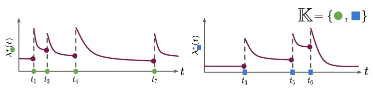
Figure 1: Illustration of a MCIF for a Hawkes process with two marks. This example highlights how events can influence the occurrence of future events. For the sake of simplicity, this illustration assumes independence between events of different marks.

Equivalently, we can fully characterize an MTPP by the joint density of inter-arrival times and marks, denoted as $f^{\ast}(\tau,k)=f(\tau,k|\mathcal{H}_{t})$, which can be dervied from the MCIF as follows:

$$f^{\ast}(\tau,k) =\lambda_{k}^{\ast}(t_{j-1}+\tau)(1-F^{\ast}(\tau))$$ (3)

$$=\lambda_{k}^{\ast}(t_{j-1}+\tau)\text{exp}\left(-\sum_{k=1}^{K}\Lambda_{k}^{\ast}(t)\right),$$ (4)

where $F^{\ast}(\tau)=\int_{0}^{\tau}\sum_{k=1}^{K}f^{\ast}(s,k)ds$ is the CDF of inter-arrival times and $\Lambda_{k}^{\ast}(t)=\int_{t_{j-1}}^{t}\lambda_{k}^{\ast}(s)ds$ is the cumulative MCIF.

We can define a valid MTPP model by specifying a parametric form $f^{\ast}(\tau,k;\bm{\theta})$, $\lambda^{\ast}_{k}(t;\bm{\theta})$ or $\Lambda^{\ast}_{k}(t;\bm{\theta})$ which defines a valid TPP probability distribution over event sequences [53]. In the framework of neural TPPs [7], such parametrizations are computed by performing three major steps, each typically involving different neural network components. Firstly, each event $\bm{e}_{j}\in\mathcal{S}$ is embedded into a representation $\bm{l}_{j}\in\mathbb{R}^{d_{l}}$. Then, a history encoder ENC generates a history embedding $\bm{h}_{j}$ for each $\bm{e}_{j}$ using its past event representations, namely $\bm{h}_{j}=\text{ENC}(\Set{\bm{l}_{j-1},\bm{l}_{j-2},,...,\bm{l}_{j-p}})\in\mathbb{R}^{d_{h}}$, where $p$ controls how far we wish to go back in the history. In essence, $\bm{h}_{j}$ acts as a neural representation of the history $\mathcal{H}_{t_{j}}$ of an event $\bm{e}_{j}$. Finally, given $\bm{h}_{j}$ and a time $t\geq t_{j-1}$, a decoder outputs the parameters of a function that uniquely characterizes the process, e.g. $f^{\ast}(\tau,k;\bm{\theta})=f(\tau,k|\bm{h}_{j};\bm{\theta})$.

Let us consider density-based neural TPP models which factorize the joint density of the inter-arrival times and mark $f(\tau,k|\bm{h};\bm{\theta})$ as $f(\tau,k|\bm{h};\bm{\theta})=f(\tau|\bm{h};\bm{\theta})p(k|\tau,\bm{h};\bm{\theta})$, where $f(\tau|\bm{h};\bm{\theta})$ is inter-arrival time PDF and $p(k|\tau,\bm{h};\bm{\theta})$ is the mark PMF given the inter-arrival time.

These density-based models are typically trained using maximum likelihood estimation (MLE). Additionally, in the context of neural TPP research, it is common to assume that the sequences in a dataset are exchangeably drawn from the underlying ground-truth TPP process. Denote $\mathcal{D}^{\ast}=\{\mathcal{S}_{1},...,\mathcal{S}_{n}\}$ the dataset containing $n$ sequences. If $\mathcal{S}_{i}=\Set{\bm{e}_{i,j}=(t_{i,j},k_{i,j)})_{j=1}^{m_{i}}}$ denotes the $i$-th sequence in $\mathcal{D}^{\ast}$ containing $m_{i}$ events observed in $[0,T]$, the negative log-likelihood (NLL) writes:

$$\mathcal{L}(\bm{\theta};\mathcal{S})=-\frac{1}{n}\sum_{i=1}^{n}\left[\sum_{j=1}^{m_{i}}\left[\text{log }f(\tau_{i,j}|\bm{h}_{i,j};\bm{\theta}))+\text{log }(p(k_{i,j}|\tau_{i,j},\bm{h}_{i,j};\bm{\theta}))\right]+\text{log }(1-F(T-t_{i,m_{i}}|\bm{h}_{i,m_{i}};\bm{\theta}))\right].$$ (5)

While the NLL has been largely adopted as the default scoring rule for learning (neural) MTPP models, [54] showed that we can define alternative (strictly) consistent loss function for $f^{\ast}(\tau,k)$ by replacing the log score in (5) with (strictly) proper scoring rules for PDFs and PMFs.

After training the neural MTTP model, $\hat{f}(\tau,k|\bm{h})$ can be used for prediction tasks for a new test sequence, addressing queries such as “When is the next event likely to occur?”, “What will be the type of the next event, given that it occurs at a certain time t?” or “How long until an event of type $k$ occurs?” [8].

4 Problem formulation and goals

Using any trained probabilistic MTPP model, we can derive a prediction region for the next arrival time, mark, or both. This region typically represents a subset of potential values that have a high probability of occurrence. However, due to model misspecification or lack of training data, the model may provide a poor approximation of the true unknown underlying process. Consequently, prediction regions derived solely from the model’s estimates may be unreliable, failing to accurately reflect the true underlying uncertainty. Building on the framework of conformal prediction (CP) [9], this paper develops more reliable methods for uncertainty quantification in neural TPP models. CP enables the construction of distribution-free prediction regions, offering a finite-sample coverage guarantee even when the base model is unreliable.

Let us consider the dataset $\mathcal{D}^{\ast}$, which is composed of $n$ sequences assumed to be drawn exchangeably from the ground-truth MTPP process. For each sequence $\mathcal{S}_{i}\in\mathcal{D}^{\ast}$, we define the input-output pair $(\bm{h}_{i,m_{i}},\bm{e}_{i,m_{i}})$, where $\bm{e}_{i,m_{i}}=(\tau_{i,m_{i}},k_{i,m_{i}})$ is a bivariate response corresponding to the last event in $\mathcal{S}_{i}$, and $\bm{h}_{i,m_{i}}$ is the history embedding associated to it. A similar scenario has been explored by [12], but for conformal time series forecasting. From these input-output pairs, we construct the dataset $\mathcal{D}=\Set{(\bm{h}_{i,m_{i}},\bm{e}_{i,m_{i}})}_{i=1}^{n}$. To simplify notation, we will henceforth denote $(\bm{h}_{i},\bm{e}_{i})=(\bm{h}_{i,m_{i}},\bm{e}_{i,m_{i}})$, implying that these quantities are consistently defined for the last event of a sequence $\mathcal{S}_{i}$.

Given $\mathcal{D}$ and a new test input $\bm{h}_{n+1}$, our primary goal is to construct an informative distribution-free joint prediction region $\hat{R}_{\tau,k}(\bm{h}_{n+1})\subseteq\mathbb{R}_{+}\times\mathbb{K}$ for the bivariate pair $\bm{e}_{n+1}=(\tau_{n+1},k_{n+1})$ of $\bm{h}_{n+1}$. This prediction region must achieve finite-sample marginal coverage at level $1-\alpha$, that is

$$\mathbb{P}((\tau_{n+1},k_{n+1})\in\hat{R}_{\tau,k}(\bm{h}_{n+1}))\geq 1-\alpha.$$ (6)

Here, the probability is taken over all $n+1$ observations, and the condition must hold true for any chosen values of $\alpha$ and $n$. Essentially, this entails developing a joint prediction region for a bivariate response, accommodating both a continuous and a categorical response, without relying on strong distributional assumptions.

We will also examine scenarios where we generate individual prediction regions for both the arrival time and the mark. Given that the arrival time is a continuous variable, we will use conformal regression techniques, while for the mark, a categorical variable, conformal classification methods will be used.

For the inter-arrival times, given $\mathcal{D}=\Set{(\bm{h}_{i},\tau_{i})}_{i=1}^{n}$ and a new test input $\bm{h}_{n+1}$, we seek to construct a prediction region $\hat{R}_{\tau}(\bm{h}_{n+1})\subseteq\mathbb{R}^{+}$ for $\tau_{n+1}$ which achieve finite-sample marginal coverage at level $1-\alpha$, that is

$$\mathbb{P}(\tau_{n+1}\in\hat{R}_{\tau}(\bm{h}_{n+1}))\geq 1-\alpha.$$ (7)

Similarly for the marks, given $\mathcal{D}=\Set{(\bm{h}_{i},k_{i})}_{i=1}^{n}$ and a new test input $\bm{h}_{n+1}$, we want to generate a prediction set $\hat{R}_{k}(\bm{h}_{n+1})\subseteq\mathbb{K}$ for $k_{n+1}$ which achieve finite-sample marginal coverage at level $1-\alpha$, that is

$$\mathbb{P}(k_{n+1}\in\hat{R}_{k}(\bm{h}_{n+1}))\geq 1-\alpha.$$ (8)

Finally, beyond ensuring a finite-sample coverage guarantee, it is essential that the prediction regions are informative, which implies striving for the smallest possible region.

To accomplish this, we will adopt the split conformal prediction framework [45], a widely used variant of CP known for its reduced computational demands. This method, which involves partitioning the data, is relatively simple but effective in transforming any heuristic notion of uncertainty into a rigorous one [43]. It enables the construction of distribution-free prediction regions that achieve finite-sample coverage guarantees. We elaborate on this methodology in the following.

Consider $\mathcal{D}=\Set{(\bm{h}_{i},\bm{y}_{i})}_{i=1}^{n}$, a dataset consisting of $n$ exchangeable pairs. In the context of our problem setup, the response $\bm{y}_{i}\in\mathcal{Y}$ varies according to the scenario: it can be bivariate as $\bm{y}_{i}=\bm{e}_{i}$ with $\mathcal{Y}=\mathbb{R}_{+}\times\mathbb{K}$, or univariate as either $\bm{y}_{i}=\tau_{i}$ or $\bm{y}_{i}=k_{i}$, with $\mathcal{Y}=\mathbb{R}_{+}$ or $\mathcal{Y}=\mathbb{K}$, respectively. Additionally, we have access to an MTPP model that provides a heuristic measure of uncertainty $\hat{g}$ for $\bm{y}$ given $\bm{h}$. The split conformal procedure can be summarized in the following steps:

1. Split $\mathcal{D}$ into two non-overlapping sets, $\mathcal{D}_{\text{train}}$ and $\mathcal{D}_{\text{cal}}$ with $\mathcal{D}_{\text{train}}\cup\mathcal{D}_{\text{cal}}=\mathcal{D}$.

2. Fit the MTPP model to the observations in $\mathcal{D}_{\text{train}}$, yielding an estimate $\hat{g}$.

3. Use $\hat{g}$ to define a non-conformity score function $s\left(\bm{h},\bm{y}\right)\in\mathbb{R}$ that assigns larger value to worse agreement between $\bm{h}$ and $\bm{y}$.

4. Compute the calibration scores using the observations in $\mathcal{D}_{\text{cal}}$, i.e. $\Set{s_{i}}_{i=1}^{|\mathcal{D}_{\text{cal}}|}:=\Set{s\left(\bm{h},\bm{y}\right):(\bm{h},\bm{y})\in\mathcal{D}_{\text{cal}}}$

5. Compute the $1-\alpha$ empirical quantile of these calibration scores:

   $$\hat{q}=\text{Quantile}\left(s_{1},...,s_{|\mathcal{D}_{\text{cal}}|}\cup\Set{\infty};\frac{\lceil(|\mathcal{D}_{\text{cal}}|+1)(1-\alpha)\rceil}{|\mathcal{D}_{\text{cal}}|}\right).$$ (9)

6. For a new test input $\bm{h}_{n+1}$, use $\hat{q}$ to construct a prediction region for $\bm{y}_{n+1}$ with a $1-\alpha$ coverage level as follows:

   $$\hat{R}_{\bm{y}}(\bm{h}_{n+1})=\Set{\bm{y}\in\mathcal{Y}:s(\bm{h}_{n+1},\bm{y})\leq\hat{q}}.$$ (10)

By the quantile lemma, we can write

$$\mathbb{P}(\bm{y}_{n+1}\in\hat{R}_{\bm{y}}(\bm{h}_{n+1}))=\mathbb{P}(s(\bm{h}_{n+1},\tau_{n+1})\leq\hat{q})\geq 1-\alpha,$$ (11)

In other words, the marginal coverage guarantees in (6), (7) and (8) are satisfied. Moreover, if no ties between the scores occur with probability one, we can further show that this marginal coverage is upper bounded, i.e.

$$1-\alpha\leq\mathbb{P}(\bm{y}_{n+1}\in\hat{R}_{\bm{y}}(\bm{h}_{n+1}))\leq 1-\alpha+\frac{1}{|\mathcal{D}_{\text{cal}}|+1}.$$ (12)

Finally, while marginal coverage is a desirable and practically achievable property, we are also interested in the stronger notion of conditional coverage:

$$\mathbb{P}(\bm{y}_{n+1}\in\hat{R}_{\bm{y}}(\bm{h}_{n+1})\mid\bm{h}_{n+1})\geq 1-\alpha\quad\forall~{}\bm{h}_{n+1},$$ (13)

which requires the desired coverage level $1-\alpha$ to be met for all $\bm{h}_{n+1}$. Despite (13) not being achievable without strong distributional assumptions [20, 21], we still aspire for the prediction regions to achieve an approximate notion of conditional coverage. The next two sections explore multiple conformal scores to achieve the guarantees in (6), (7) and (8).

5 Individual prediction regions for arrival times and marks

In this section, we outline the methods for generating individual prediction regions $\hat{R}_{\tau}({\bm{h}_{n+1}})$ and $\hat{R}_{k}({\bm{h}_{n+1}})$ for $\tau_{n+1}$ and $k_{n+1}$, respectively. As $\tau_{n+1}$ is a continuous variable, we rely on conformal regression techniques to construct $\hat{R}_{\tau}({\bm{h}_{n+1}})$. Conversely, $k_{n+1}$ being a categorical variable, we leverage conformal classification approaches to build $\hat{R}_{k}({\bm{h}_{n+1}})$.

5.1 Constructing a prediction region for the arrival time

Using a dataset $\mathcal{D}=\Set{(\bm{h}_{i},\tau_{i})}_{i=1}^{n}$, our objective is to construct a prediction region $\hat{R}_{\tau}(\bm{h}_{n+1})\subseteq\mathbb{R}^{+}$ for the arrival time $\tau_{n+1}$ of a new test input $\bm{h}_{n+1}$. This prediction region must achieve finite-sample marginal coverage at level $1-\alpha$, as given in (7). An intuitive approach is to create an equal-tailed prediction interval using conditional quantiles at levels $\nicefrac{{\alpha}}{{2}}$ and $1-\nicefrac{{\alpha}}{{2}}$. Let $\hat{Q}_{\tau}(\cdot|\bm{h})$ be the predictive quantile function of $\tau$ given $\bm{h}$ trained using $\mathcal{D}$. We can define a symmetric prediction interval for $\tau_{n+1}$ as:

$$\hat{R}_{\tau}(\bm{h}_{n+1})=[\hat{Q}_{\tau}(\nicefrac{{\alpha}}{{2}}|\bm{h}_{n+1}),\hat{Q}_{\tau}(1-\nicefrac{{\alpha}}{{2}}|\bm{h}_{n+1})],$$ (14)

However, as previously mentioned, there is no guarantee that the estimate $\hat{Q}_{\tau}(\cdot|\bm{h}_{n+1})$ is a good approximation of the true $Q^{*}_{\tau}(\cdot|\bm{h}_{n+1})$, resulting in no finite-sample coverage guarantee. By adjusting (14), Conformalized Quantile Regression (C-QR) can provide a symmetric prediction interval with a finite-sample coverage guarantee (see Theorem 2 in[17]). For a symmetric prediction interval given by (14), the CQR nonconformity score can be defined as

$$s_{\text{CQR}}(\bm{h},\tau)=\text{max}\left(\hat{Q}_{\tau}(\nicefrac{{\alpha}}{{2}}|\bm{h})-\tau,\tau-\hat{Q}_{\tau}(1-\nicefrac{{\alpha}}{{2}}|\bm{h})\right),$$ (15)

and accounts for both potential undercoverage and overcoverage from the model. Indeed, the further $\tau$ falls outside of the interval $\hat{R}_{\tau}(\bm{h}_{n+1})$ in (14), the greater is the positive value of $s_{\text{CQR}}$. Conversely, $s_{\text{CQR}}$ decreases the further $\tau$ correctly falls within the interval $\hat{R}_{\tau}(\bm{h}_{n+1})$. After evaluating $s_{\text{CQR}}$ on hold-out calibration samples and computing $\hat{q}$ using (9), we construct a valid prediction interval for $\tau_{n+1}$ as:

$$\hat{R}_{\tau,\text{CQR}}(\bm{h}_{n+1})=[\hat{Q}_{\tau}(\nicefrac{{\alpha}}{{2}}|\bm{h}_{n+1})-\hat{q},\hat{Q}_{\tau}(1-\nicefrac{{\alpha}}{{2}}|\bm{h}_{n+1})+\hat{q}],$$ (16)

which satisfies marginal coverage at level $1-\alpha$ since

$$\mathbb{P}(\tau_{n+1}\in\hat{R}_{\tau}(\bm{h}_{n+1}))=\mathbb{P}(s_{\text{CQR}}(\bm{h}_{n+1},\tau_{n+1})\leq\hat{q})\geq 1-\alpha.$$ (17)

However, since the strictly positive arrival times often show a skewed distribution with a significant concentration of probability mass close to 0, this method would not encompass the high-density region between levels 0 and $\nicefrac{{\alpha}}{{2}}$, and thus would lead to unnecessarily large intervals. Therefore, a more effective strategy involves generating an asymmetric interval extending from level 0 to $\alpha$, where the lower bound of the interval remains fixed at 0, and the upper bound, or the right tail, is independently adjusted. This translates into the following asymmetric prediction interval for $\tau_{n+1}$:

$$\hat{R}_{\tau}(\bm{h}_{n+1})=[0,\hat{Q}_{\tau}(1-\alpha|\bm{h}_{n+1})],$$ (18)

for which we define a Conformalized Quantile Regression Left (C-QRL) nonconformity score, expressed as:

$$s_{\text{CQRL}}(\bm{h},\tau)=\tau-\hat{Q}_{\tau}(1-\alpha|\bm{h}).$$ (19)

Naturally, this score inherits the same interpretation as the one of C-QR, and leads to the following asymmetric prediction region after estimating $\hat{q}$ on the calibration samples:

$$\hat{R}_{\tau,\text{CQRL}}(\bm{h}_{n+1})=[0,\hat{Q}_{\tau}(1-\alpha|\bm{h}_{n+1})+\hat{q}],$$ (20)

Additionally, it is worth noting that both $s_{\text{CQR}}$ and $s_{\text{CQRL}}$ can be directly computed from the cumulative MCIF:

$$\hat{Q}_{\tau}(\alpha|\bm{h})=\hat{\Lambda}^{-1}\left(-\text{log }(1-\alpha)|\bm{h}\right)-t_{j-1},$$ (21)

where we reused the notations of Section 3 to indicate that $t_{j-1}$ is the last observed event arrival time in $\mathcal{H}_{t}$. Moreover, if the estimators of the quantiles are consistent (that is, they converge to the true conditional quantiles as the sample size increases), C-QR and C-QRL have asymptotic conditional coverage, and therefore (13) will hold approximately if $n$ is large [55, Corolary 1]. As alternatives to C-QR and C-QRL for constructing prediction intervals for $\tau_{n+1}$, one could instead leverage the approaches of Conformal Histogram Regression (CHR) [56] or HPD-Split [16]. While we expand further on HPD-split in a later section, we leave CHR as inquiry for future work.

5.2 Constructing a prediction set for the mark

Using a dataset $\mathcal{D}=\Set{(\bm{h}_{i},k_{i})}_{i=1}^{n}$, our objective is to construct a prediction set $\hat{R}_{k}(\bm{h}_{n+1})\subseteq\mathbb{K}$ for the mark $k_{n+1}$ of a new test input $\bm{h}_{n+1}$. This prediction set must achieve finite-sample marginal coverage at level $1-\alpha$, as given in (8).

Let $\hat{p}(\cdot|\bm{h})$ denote the predictive PMF of $k$ given $\bm{h}$, trained using $\mathcal{D}$. To generate a prediction set for $k_{n+1}$, a simple method involves ranking the marks in descending order by their associated conditional probabilities and retaining those marks where the cumulative sum of these probabilities is less than or equal to the pre-specified probability coverage. However, as previously mentioned, there is no guarantee that we have a good approximation of the true conditional probabilities $p^{*}(\cdot|\bm{h})$.

Furthermore, MTPPs often involve a large number of marks, for example, up to $|\mathbb{K}|=50$ in our experiments, yet in practice, only a few of these marks hold significant probability. Identifying and focusing on these high-probability marks is essential as it leads to more informative prediction sets. This is the rationale behind the method of conformal Adaptive Prediction Sets (APS) [18]. We focus on the more recent method of Regularized Adaptive Prediction Sets (RAPS) [19], which consistently generates prediction sets of smaller size than APS by introducing regularization.

Specifically, given $\hat{p}(\cdot|\bm{h})$, RAPS defines the following nonconformity score:

$$s_{\text{RAPS}}(\bm{h},k)=\sum_{{k^{\prime}:\hat{p}(k^{\prime}|\bm{h})\geq\hat{p}(k|\bm{h})}}\hat{p}(k^{\prime}|\bm{h})+u\cdot\hat{p}(k|\bm{h})+\gamma\left(o(k)-k_{\text{reg}}\right)^{+},$$ (22)

where $u$ is a uniform random variable handling discrete jumps in the cumulative sum of $\hat{p}(k|\bm{h})$, and $o(k)=|\Set{k^{\prime}\in\mathbb{K}:\hat{p}(k^{\prime}}{\bm{h})\geq\hat{p}(k|\bm{h})}|$ is the ranking of the observed mark $k$ among the probabilities in $\hat{p}(\cdot|\bm{h})$. In (22), $(x)^{+}$ further denotes the positive part of $x$, and $\gamma,k_{\text{reg}}\geq 0$ are regularization parameters that help promote smaller set sizes compared to the ones generated by APS, which nonconformity score can be easily recovered by setting $\gamma=0$ in (22). Minus the randomization and regularization terms, the RAPS score essentially computes the cumulative sum of mark probabilities that are greater or equal to the probability of the observed ground-truth mark $k$. If we had knowledge of the true PMF, we could construct a prediction set for $k_{n+1}$ as

$$\hat{R}_{k}(\bm{h}_{n+1})=\Set{k^{\prime}\in\mathbb{K}:s_{\text{RAPS}}(\bm{h}_{n+1},k^{\prime})\leq 1-\alpha},$$ (23)

that would meet the required marginal coverage of $1-\alpha$. Instead, the split conformal procedure introduced in Section 3 first computes the RAPS scores on a hold-out calibration set $\mathcal{D}_{cal}$. Then, having computed the adjusted $1-\alpha$ quantile $\hat{q}$ for these scores from (9), we construct the following prediction set for $k_{n+1}$:

$$\hat{R}_{k}(\bm{h}_{n+1})=\Set{k^{\prime}\in\mathbb{K}:s_{\text{RAPS}}(\bm{h}_{n+1},k^{\prime})\leq\hat{q}},$$ (24)

which satisfies the desired marginal coverage guarantee at level $1-\alpha$ since

$$\mathbb{P}(k_{n+1}\in\hat{R}_{k}(\bm{h}_{n+1}))=\mathbb{P}(s_{\text{RAPS}}(\bm{h}_{n+1},k_{n+1})\leq\hat{q})\geq 1-\alpha.$$ (25)

Finally, it is worth noting that the APS/RAPS scores can be derived from the MCIF by recovering the marginal conditional probabilities using the following definition:

$$p(k|\bm{h})=\mathbb{E}_{\tau}\left[\frac{\hat{\lambda}_{k}(t_{j-1}+\tau|\bm{h})}{\hat{\lambda}(t_{j-1}+\tau|\bm{h})}\right].$$

6 Joint prediction regions for the arrival times and marks

Working with a dataset $\mathcal{D}=\Set{(\bm{h}_{i},\bm{e}_{i})}_{i=1}^{n}$ where $\bm{e}_{i}=(\tau_{i},k_{i})$, our aim is to construct an informative, distribution-free joint prediction region $\hat{R}_{\tau,k}(\bm{h}_{n+1})\in\mathbb{R}^{+}\times\mathbb{K}$ for the pair $(\tau_{n+1},k_{n+1})$ associated with a new test input $\bm{h}_{n+1}$. This prediction region should satisfy finite-sample marginal coverage at level $1-\alpha$, as given by (6). Essentially, this involves generating a joint prediction region for a bivariate response, which integrates a continuous and a categorical variable, without relying on distributional assumptions.

In the following section, we will first explore a naive yet statistically sound method that combines individual prediction regions for the event arrival time and the mark, as outlined in Section 5. However, by neglecting potential dependencies between these variables, this method can be overly conservative, resulting in large prediction regions which would not reflect the true underlying uncertainty. A more effective strategy involves jointly predicting the event arrival time and the mark, which will better reflect the true distribution of these two variables. The associated joint prediction region can then exclude unlikely combinations of the two, while still attaining the pre-specified coverage level.

As discussed in Section 2, the body of literature on conformal prediction for multi-response scenarios is limited, with notable contributions including [13] and [14]. However, [13] propose a method centered on multi-output quantile regression for continuous random vectors, which is not easily applicable in our context. Additionally, while [14] does present a density-based conformal method, it is not suited for estimation problems involving covariates. Instead, we explore an adaptation of the univariate HPD-split method [16] for bivariate responses. This method enables us to construct highest density regions using the joint predictive density of event arrival time and mark.

6.1 Combining individual conformal prediction regions

Let $\hat{R}_{\tau}(\bm{h}_{n+1})\subseteq\mathbb{R}^{+}$ and $\hat{R}_{k}(\bm{h}_{n+1})\subseteq\mathbb{K}$ represent the prediction regions for the arrival time $\tau_{n+1}$ and the mark $k_{n+1}$, respectively, for a new test input $\bm{h}_{n+1}$, as described in Section 5. Furthermore, the nominal coverage level for these two regions, specifically the right-hand side of equations (7) and (8), is set to $1-\nicefrac{{\alpha}}{{2}}$. Then, the joint prediction region $\hat{R}_{\tau,k}(\bm{h}_{n+1})=\hat{R}_{\tau}(\bm{h}_{n+1})\times\hat{R}_{k}(\bm{h}_{n+1})\subseteq\mathbb{R}^{+}\times\mathbb{K}$ for $(\tau_{n+1},k_{n+1})$ obtained by combining these two regions has coverage at least $1-\alpha$. In fact, by the union bound, we have:

$$\mathbb{P}((\tau_{n+1},k_{n+1})\in\hat{R}_{\tau}(\bm{h}_{n+1})\times\hat{R}_{k}(\bm{h}_{n+1})) =\mathbb{P}(\tau_{n+1}\in\hat{R}_{\tau}(\bm{h}_{n+1})\cap k_{n+1}\in\hat{R}_{k}(\bm{h}_{n+1}))$$ (26)

$$=1-\underbrace{\mathbb{P}(\tau_{n+1}\not\in\hat{R}_{\tau}(\bm{h}_{n+1})\cup k_{n+1}\not\in\hat{R}_{k}(\bm{h}_{n+1}))}_{\leq\nicefrac{{\alpha}}{{2}}+\nicefrac{{\alpha}}{{2}}}$$ (27)

$$\geq 1-\alpha.$$ (28)

However, this method, which treats the arrival time $\tau$ and the mark $k$ separately, can be overly conservative, resulting in large and inflexible prediction regions. Indeed, the joint prediction region generated by this approach yields equal length prediction intervals for the arrival times across all selected marks, i.e.:

$$\hat{R}_{\tau,k}(\bm{h}_{n+1})=\{(\tau^{\prime},k^{\prime})|\tau^{\prime}\in\hat{R}_{\tau}(\bm{h}_{n+1}),k^{\prime}\in\hat{R}_{k}(\bm{h}_{n+1})\}=\{\tau^{\prime}|\tau^{\prime}\in\hat{R}_{\tau}(\bm{h}_{n+1})\}\times\{k^{\prime}|k^{\prime}\in\hat{R}_{k}(\bm{h}_{n+1})\}.$$ (29)

In other words, for each of the selected marks in $\hat{R}_{k}(\bm{h}_{n+1})$, the same prediction interval is constructed for $\tau_{n+1}$. In the following, we refer to this approach as Conformal Independent (C-IND). Fig. 2(a) shows an example of creating such prediction region. First, a region $\hat{R}_{\tau}(\bm{h}_{n+1})$ is constructed for $\tau_{n+1}$ at level $1-\frac{\alpha}{2}$ (bottom of the figure). Then, a region $\hat{R}_{k}(\bm{h}_{n+1})$ is constructed for $k_{n+1}$, also at level $1-\frac{\alpha}{2}$ (right side of the figure), and finally, $\hat{R}_{k}(\bm{h}_{n+1})$ is obtained by taking the cartesian product between the two regions.

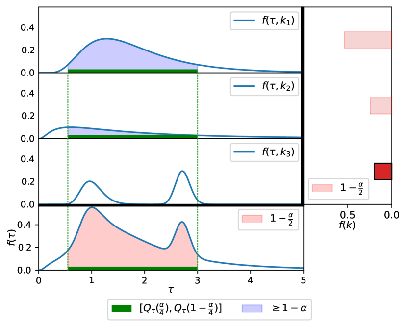
((a)) The joint region obtained by combining CQR for the time with coverage $1-\frac{\alpha}{2}$ and APS for the mark with coverage $1-\frac{\alpha}{2}$ will have a coverage greater than $1-\alpha$.

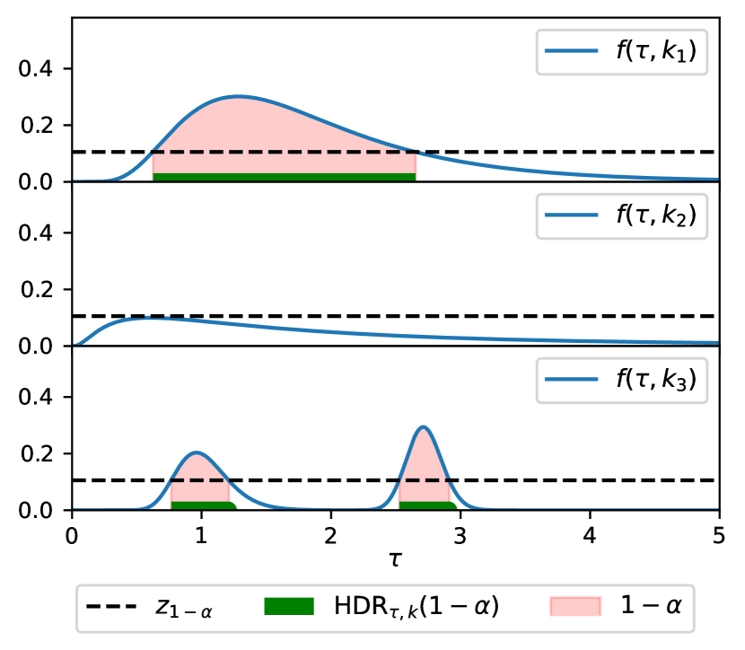
((b)) In contrast to the approach of combining individual prediction regions for the time and mark, HDR can produce different regions $\hat{R}_{\tau}^{(k_{1})}(\bm{h}_{n+1})$ and $\hat{R}_{\tau}^{(k_{3})}(\bm{h}_{n+1})$ depending on the mark. It also demonstrates the ability to exclude marks by producing an empty set $\hat{R}_{\tau}^{(k_{2})}(\bm{h}_{n+1})$.

Figure 2: Example of joint prediction regions with $\alpha=0.4$ on a synthetic example with $\tau\in\mathbb{R}^{+}$ and three marks $k_{1}$, $k_{2}$ and $k_{3}$.

6.2 Conformal highest joint density regions

A better strategy for generating a joint prediction region for the arrival time and the mark involves leveraging their joint distribution. By doing so, this approach excludes unlikely combinations of the two variables, while achieving the pre-specified coverage level. To accomplish this, we propose to compute the highest density region (HDR, [15]) with a nominal coverage level of $1-\alpha$, based on the joint density of the arrival time and mark. Let $\hat{f}(\tau,k|\bm{h}_{n+1})$ denote this predictive joint density for a new test point $\bm{h}_{n+1}$. The HDR of $\hat{f}$ with nominal coverage level $1-\alpha$ is defined as:

$$\text{HDR}(1-\alpha|\bm{h}_{n+1})=\Set{(\tau,k)}{\hat{f}(\tau,k|\bm{h}_{n+1})\geq z_{1-\alpha}},$$ (30)

where

$$z_{1-\alpha}=\text{sup}\Set{z^{\prime}}{\mathbb{P}(\hat{f}(\tau,k|\bm{h}_{n+1})\geq z^{\prime})\geq 1-\alpha}.$$ (31)

It is important to highlight that in cases where the underlying distribution exhibits multimodality, an HDR approach will result in a union of intervals that, collectively, are shorter in length than a single interval with the same coverage level. Specifically, the oracle HDR has the useful property of generating the smallest possible region that guarantees conditional coverage.

Moreover, in contrast to the C-IND method outlined in the previous section, an HDR approach can produce prediction regions for the arrival time that vary in length across different selected marks. Specifically, the joint HDR can be expressed as

$$\hat{R}_{\tau,k}(\bm{h}_{n+1})=\text{HDR}(1-\alpha|\bm{h}_{n+1})=\bigcup_{k^{{}^{\prime}}\in\hat{R}_{k}(\bm{h}_{n+1})}\{(\tau^{\prime},k^{\prime})|\tau^{\prime}\in\hat{R}_{\tau}^{(k^{\prime})}(\bm{h}_{n+1})\},$$ (32)

where

$$\hat{R}_{k}(\bm{h}_{n+1})=\{k^{\prime}|\exists~{}\tau\in\mathbb{R}^{+}:\hat{f}(\tau,k^{\prime}|\bm{h}_{n+1})\geq z_{1-\alpha}\},\quad\text{and}\quad\hat{R}_{\tau}^{(k)}(\bm{h}_{n+1})=\{\tau^{\prime}|\hat{f}(\tau^{\prime},k|\bm{h}_{n+1})\geq z_{1-\alpha}\}.$$ (33)

In simpler terms, $\hat{R}_{k}(\bm{h}_{n+1})$ encompasses all marks $k\in\mathbb{K}$ for which $\hat{f}(\tau,k|\bm{h}_{n+1})$ exceeds $z_{1-\alpha}$ over any non-zero interval in $\mathbb{R}_{+}$. Subsequently, for each $k^{\prime}\in\hat{R}_{k}(\bm{h}_{n+1})$, $\hat{R}_{\tau}^{(k)}(\bm{h}_{n+1})$ contains the range of $\tau$ values where the joint distribution $\hat{f}(\tau,k|\bm{h}_{n+1})$ surpasses the threshold $z_{1-\alpha}$. This shows that the HDR is capable of adapting to the joint distribution of the arrival time and mark, leading to more tailored and potentially more efficient prediction regions than (29).

Figure 2(b) illustrates the HDR for a simplified example with $\mathbb{K}=\{k_{1},k_{2},k_{3}\}$. The various prediction sets constituting the HDR are as follows: $\hat{R}_{k}(\bm{h}_{n+1})=\{k_{1},k_{3}\}$, referring to the selected marks; $\hat{R}_{\tau}^{(k_{1})}(\bm{h}_{n+1})=[0.8,2.6]$ and $\hat{R}_{\tau}^{(k_{3})}(\bm{h}_{n+1})=[0.8,1.2]\cup[2.5,2.9]$, referring to the arrival time intervals associated to marks $k_{1}$ and $k_{3}$, respectively. Finally, $\hat{R}_{\tau}^{(k_{2})}(\bm{h}_{n+1})=\emptyset$, indicating that mark $k_{2}$ is not selected in this scenario.

Unfortunately, the joint prediction region presented in (32) does not come with a finite-sample coverage guarantee. To address this, we modify the nominal coverage level $1-\alpha$ of the HDR by using a generalization of the univariate HPD-split conformal procedure [16]. We refer to this approach as Conformal HDR (C-HDR).

Let $\hat{q}\in[0,1]$. For a new test input $\bm{h}_{n+1}$, and as per the definition of HDR in (30), it holds that

$$(\tau_{n+1},k_{n+1})\in\text{HDR}(\hat{q}|\bm{h}_{n+1})\iff\text{HPD}(\tau_{n+1},k_{n+1}|\bm{h}_{n+1})\leq\hat{q},$$

where

$$\text{HPD}(\tau,k|\bm{h})=\sum_{k^{\prime}\in\mathbb{K}}\int_{\Set{\tau^{\prime}}{\hat{f}(\tau^{\prime},k^{\prime}|\bm{h})\geq\hat{f}(\tau,k|\bm{h})}}\hat{f}(\tau^{\prime},k^{\prime}|\bm{h})d\tau,$$

effectively calculates the probability coverage of pairs $(\tau^{\prime},k^{\prime})$ having a higher density than $(\tau,k)$. The C-HDR method defines nonconformity scores based on HPD values,

$$s_{\text{HPD}}(\bm{h},(\tau,k))=\text{HPD}(\tau,k|\bm{h}),$$ (34)

and returns a joint HDR with an adjusted nominal coverage level $\hat{q}$, computed as the $1-\alpha$ empirical quantile of the $s_{\text{HPD}}$ scores evaluated on $\mathcal{D}_{\text{cal}}$, i.e.

$$\hat{R}_{\tau,k}(\bm{h}_{n+1})=\text{HDR}(\hat{q}|\bm{h}_{n+1}).$$ (35)

Furthermore, the quantile lemma ensures that this prediction region verifies the conformal guarantee at nominal level $1-\alpha$, i.e.

$$\mathbb{P}((\tau_{n+1},k_{n+1})\in\hat{R}_{\tau,k}(\bm{h}_{n+1}))=\mathbb{P}(s_{\text{HPD}}(\bm{h}_{n+1},(\tau_{n+1},k_{n+1}))\leq\hat{q})\geq 1-\alpha.$$ (36)

Moreover, if the estimator of $\hat{f}$ is consistent (that is, it converges to the true $f$ as the sample size increases), the C-HDR nonconformity scores are approximately independent of the input features, which leads to asymptotic conditional coverage. That is, (13) will hold approximately if $n$ is large [16, Theorem 27]. Moreover, under these assumptions, C-HDR will also converge to the smallest prediction region that achieves conditional coverage of $1-\alpha$ [16, Theorem 27].

7 Experiments

We assess the validity and statistical efficiency of the prediction regions produced by various CP methods, as detailed in Sections 5 and 6. Our evaluation is based on five marked event sequence datasets from real-world scenarios, which have been previously considered in neural TPP research. Below, we provide a description of these datasets:

• LastFM [57]: This dataset comprises records of individuals’ song-listening events over time, with each song’s artist serving as the mark.

• MOOC [57]: It captures the activities of students on an online course platform, where the mark denotes the specific type of activity, such as watching a video.

• Reddit [57]: This consists of sequences of posts made to various subreddits. Each sequence is associated with a user, and the mark is the post that the user responds to.

• Retweets [30]: It includes sequences of retweets occurring after an initial tweet over time. Each sequence is linked to a specific tweet, with the mark being a category assigned to the retweeter (small, medium, or large retweeter).

• Stack Overflow [26]: This dataset records the badges awarded to users on Stack Overflow. Each user is assigned a sequence, and the type of badge received is used as the mark.

Following [8], we preprocess each dataset to include only its 50 most frequently occurring marks. Additionally, to prevent numerical instabilities, we normalized the arrival times of events to fall within the range of $[0,10]$. Detailed summary statistics of these pre-processed real-world datasets are presented in Table 1.

	#Seq.	#Events	Mean Length	Max Length	Min Length	#Marks
LastFM	856	193441	226.0	6396	2	50
MOOC	7047	351160	49.8	416	2	50
Reddit	4278	238734	55.8	941	2	50
Retweets	12000	1309332	109.1	264	50	3
Stack Overflow	7959	569688	71.6	735	40	22

Table 1: Real-world datasets statistics

In addition to the real-world data, we also created a synthetic dataset using a multi-dimensional Hawkes process with exponential kernels [5]. We set the MCIF parameters in (2) to align with the values used in [8], as follows:

$$\bm{\mu}=\begin{pmatrix}0.2\\ 0.6\\ 0.1\\ 0.7\\ 0.9\end{pmatrix}\qquad\bm{\alpha}=\begin{pmatrix}0.25&0.13&0.13&0.13&0.13\\ 0.13&0.35&0.13&0.13&0.13\\ 0.13&0.13&0.2&0.13&0.13\\ 0.13&0.13&0.13&0.3&0.13\\ 0.13&0.13&0.13&0.13&0.25\end{pmatrix}\qquad\bm{\beta}=\begin{pmatrix}4.1&0.5&0.5&0.5&0.5\\ 0.5&2.5&0.5&0.5&0.5\\ 0.5&0.5&6.2&0.5&0.5\\ 0.5&0.5&0.5&4.9&0.5\\ 0.5&0.5&0.5&0.5&4.1\end{pmatrix}.$$

This configuration results in a marked process with $K=5$ marks. We generated five distinct Hawkes datasets, each containing 14,408 sequences, with the tick library [58]. For all datasets, we randomly divided the sequences into training ($\mathcal{D}_{\text{train}}$), validation ($\mathcal{D}_{\text{val}}$), calibration ($\mathcal{D}_{\text{cal}}$), and test ($\mathcal{D}_{\text{test}}$) splits, in proportions of 65%, 10%, 15%, and 10%, respectively.

7.1 Heuristic and conformal prediction methods

We first focus on creating distinct univariate prediction regions for the event arrival time and the event mark of new test inputs. This is achieved through the application of conformal regression and classification techniques, as detailed in Section 5. Additionally, we explore CP methods for constructing bivariate prediction regions for both the event arrival time and its associated mark, as described in Section 6. Finally, we also consider heuristic versions, which correspond to non-conformal versions of these methods, by simply replacing the model estimate in the corresponding oracle prediction region. We provide a summary of these methods below.

Prediction regions for the event arrival time. We explore various methods to generate a prediction region for $\tau_{n+1}$ of a test input $\bm{h}_{n+1}$, targeting marginal coverage $1-\alpha$. For the heuristic methods, the first baseline is Heuristic QR (H-QR), which constructs a symmetric interval centered at the median:

$$\hat{R}_{\tau,\text{H-QR}}(\bm{h}_{n+1})=[\hat{Q}_{\tau}(\alpha|\bm{h}_{n+1}),\hat{Q}_{\tau}(1-\alpha|\bm{h}_{n+1})].$$ (37)

The second baseline is Heuristic QRL (H-QRL), which generates an asymmetrical interval with the left bound at zero:

$$\hat{R}_{\tau,\text{H-QRL}}(\bm{h}_{n+1})=[0,\hat{Q}_{\tau}(1-\alpha|\bm{h}_{n+1})].$$ (38)

The third baseline is Heuristic HDR (H-HDR) which forms a HDR, i.e.

$$\hat{R}_{\tau,\text{H-HDR}}(\bm{h}_{n+1})=\{\tau|\hat{f}(\tau|\bm{h}_{n+1})\geq z_{1-\alpha}\},$$ (39)

where $z_{1-\alpha}=\text{sup}\Set{z^{\prime}}{\mathbb{P}(\hat{f}(\tau|\bm{h}_{n+1})\geq z^{\prime})\geq 1-\alpha}$. Unlike the HDR defined in (30) for a joint prediction on the time and mark, this method represents a univariate HDR, specifically focusing on the arrival time.

We also consider conformal versions of these approaches, denoted as C-QR, C-QRL, and C-HDR, with prediction regions defined in equations (16), (20), and (35), respectively. Additionally, we analyze C-CONST, a simple conformal baseline. Its nonconformity score is defined as $s_{\text{C}}(\bm{h},\tau)=\tau$ and it generates predictions regions of the form $\hat{R}_{\tau}(\bm{h}_{n+1})=[0,\hat{q}]$, independent of the model and history $\bm{h}$, where $\hat{q}$ is defined by the split-conformal prediction algorithm in (9).

Prediction sets for the event mark. We explore various methods to generate a prediction set for $k_{n+1}$ given a test input $\bm{h}_{n+1}$. The first baseline methods, called Heuristic APS (H-APS) and Heuristic RAPS (H-RAPS), generate the following sets:

$$\hat{R}_{k,\text{H-APS}}(\bm{h}_{n+1})=\Set{k^{\prime}\in\mathbb{K}:s_{\text{APS}}(\bm{h}_{n+1},k^{\prime})\leq 1-\alpha},$$ (40)

and

$$\hat{R}_{k,\text{H-RAPS}}(\bm{h}_{n+1})=\Set{k^{\prime}\in\mathbb{K}:s_{\text{RAPS}}(\bm{h}_{n+1},k^{\prime})\leq 1-\alpha}.$$ (41)

For their conformal counterparts, we derive prediction regions as detailed in (24) and the unregularized C-APS algorithm described in [18]. Recall that $s_{\text{APS}}$ is recovered from $s_{\text{RAPS}}$ by setting $\gamma=0$ in (22). Additionally, we explore the C-PROB conformal baseline, introduced in [43]. This baseline defines its nonconformity score in terms of the estimated probability mass function over the mark:

$$s_{\text{C-PROB}}(\bm{h},k)=1-\hat{p}(k|\bm{h}),$$ (42)

which yields the following prediction region after computing $\hat{q}$ with the split-conformal prediction algorithm (9):

$$\hat{R}_{k,\text{C-PROB}}(\bm{h}_{n+1})=\Set{k^{\prime}\in\mathbb{K}:\hat{p}(k^{\prime}}{\bm{h})\geq 1-\hat{q}}.$$ (43)

Moreover, to avoid the generation of empty prediction sets, the mark associated to the highest estimated probability is systematically included for all methods that we consider, namely H-APS, H-RAPS, C-PROB, C-APS and C-RAPS.

Bivariate prediction regions for the arrival time and the associated mark. We explore two methodologies to construct a bivariate prediction region, $\hat{R}_{\tau,k}(\bm{h}_{n+1})$, for the pair $(\tau_{n+1},k_{n+1})$. The first method combines individual univariate prediction regions, as detailed in Section 6.1. For this method, we develop two variants, each based on the specific construction of $\hat{R}_{\tau}(\bm{h}_{n+1})$ and $\hat{R}_{k}(\bm{h}_{n+1})$. The first variant, C-QRL-RAPS, combines C-QRL for $\hat{R}_{\tau}(\bm{h}_{n+1})$ and C-RAPS for $\hat{R}_{k}(\bm{h}_{n+1})$. The second variant, C-HDR-RAPS, uses C-HDR for $\hat{R}_{\tau}(\bm{h}_{n+1})$, while still employing C-RAPS for $\hat{R}_{k}(\bm{h}_{n+1})$. The second method generates joint HDR regions, as described in Section 6.2. In parallel, we also examine their heuristic counterparts, referred to as H-QRL-RAPS, H-HDR-RAPS, and H-HDR, respectively.

7.2 Neural TPP models

We present several SOTA neural TPP models designed to estimate the joint density of event arrival time and mark, represented as $\hat{f}(\tau,k|\bm{h})$. From these models, we will derive a heuristic-based measure of uncertainty. Recall that given a sequence of events $\mathcal{S}=\Set{\bm{e}_{1},...,\bm{e}_{m}}$, these models can be essentially decomposed into three main components: an event encoder, a history encoder, and a decoder. To obtain an event representation $\bm{l}_{j}\in\mathbb{R}^{d_{e}}$ for $\bm{e}_{j}=(t_{j},k_{j})$, we proceed in two steps. First, we follow [1] by mapping $t_{j}$ to a vector of sinusoidals functions [1]:

$$\bm{l}^{t}_{j}=\underset{s=0}{\overset{d_{t}/2-1}{\bigoplus}}\text{sin}~{}(\alpha_{s}t_{j})\oplus\text{cos}~{}(\alpha_{s}t_{j})\in\mathbb{R}^{d_{t}},$$ (44)

where $\alpha_{s}\propto 1000^{\frac{-2s}{d_{t}}}$ and $\oplus$ is the concatenation operator. Then, a mark embedding $\bm{l}_{j}^{k}\in\mathbb{R}^{d_{k}}$ for $k_{j}$ is computed as $\bm{l}_{j}^{k}=\mathbf{E}^{k}\bm{k}_{j}$, where $\mathbf{E}^{k}\in\mathbb{R}^{d_{k}\times K}$ is a learnable embedding matrix, and $\bm{k}_{j}\in\{0,1\}^{K}$ is the one-hot encoding of $k_{j}$. The event representation $\bm{l}_{j}$ is finally obtained through concatenation, i.e. $\bm{e}_{j}=[\bm{e}_{j}^{t}\oplus\bm{e}_{j}^{k}]$. Subsequently, we generate the history embedding $\bm{h}_{j}\in\mathbb{R}^{d_{h}}$ of an event $\bm{e}_{j}$ by sequentially processing its set of past events representations through a GRU encoder:

$$\bm{h}_{j}=\text{GRU}\left(\Set{\bm{l}_{1},...,\bm{l}_{j-1}}\right).$$ (45)

Finally, given $\bm{h_{j}}$ and a query time $t>t_{j-1}$, we consider several decoders which computes either $\hat{f}(\tau,k|\bm{h}_{j})$, $\hat{\lambda}_{k}(t|\bm{h}_{j})$, or $\hat{\Lambda}_{k}(t|\bm{h}_{j})$. Recall that each of these functions can be retrieved from the others through (4). We describe four different decoders below.

• Conditional LogNormMix (CLNM) [31, 59] models $\hat{f}(\tau,k|\bm{h}_{j})=\hat{f}(\tau|\bm{h_{j}})\hat{p}(k|\tau,\bm{h}_{j})$ with $\hat{f}(\tau|\bm{h}_{j})$ being a mixture of log-normal distributions:

  $$\hat{f}(\tau|\bm{h}_{j})=\sum_{c=1}^{C}p_{c}\frac{1}{\tau\sigma_{c}\sqrt{2\pi}}\text{exp}\Big{(}-\frac{(\text{log}~{}\tau-\mu_{c})^{2}}{2\sigma_{c}^{2}}\Big{)},$$ (46)

  where $p_{c}=\text{Softmax}\big{(}\mathbf{W}_{p}\bm{h}_{j}+\bm{b}_{p}\big{)}_{c}$, $\mu_{c}=(\mathbf{W}_{\mu}\bm{h}_{j}+\bm{b}_{\mu})_{c}$, and $\sigma_{c}=\text{exp}(\mathbf{W}_{\sigma}\bm{h}_{j}+\bm{b}_{\sigma})_{c}$ are the weight, mean and standard deviation of the $c^{th}$ mixture component, respectively. In (46), $\mathbf{W}_{p},\mathbf{W}_{\mu},\mathbf{W}_{\sigma}\in\mathbb{R}^{C\times d_{h}}$ and $\bm{b}_{p},\bm{b}_{\mu},\bm{b}_{\sigma}\in\mathbb{R}^{C}$ with $C$ being the number of mixture components. The mark PMF is given by

  $$\hat{p}(k|\tau,\bm{h}_{j})=\sigma_{S}\left(\mathbf{W}_{2}\sigma_{R}\left(\mathbf{W}_{1}\left[\bm{h}_{j}\oplus\text{log }\tau\right]+\bm{b}_{1})\right)+\bm{b}_{2}\right),$$ (47)

  where $\mathbf{W}_{1}\in\mathbb{R}^{d_{1}\times(d_{h}+1)}$, $\bm{b}_{1}\in\mathbb{R}^{d_{1}}$, $\mathbf{W}_{2}\in\mathbb{R}^{K\times d_{1}}$, and $\bm{b}_{2}\in\mathbb{R}^{K}$.
  

• FullyNN (FNN) [30, 1] directly parametrizes the cumulative MCIF as follows:

  $$\hat{\Lambda}_{k}^{\ast}(t)=G_{k}^{\ast}(t)-G_{k}^{\ast}(t_{j-1}),$$ (48)

  $$G_{k}^{\ast}(t)=\sigma_{S,k}\big{(}\bm{w}_{k}^{\mathsf{T}}(\sigma_{GS,k}\big{(}\bm{w}^{t}\text{log }\tau+\mathbf{W}^{h}\bm{h}_{j}+\bm{b}\big{)}+b_{k}\big{)},$$ (49)

  where $\sigma_{S,k}$ and $\sigma_{GS,k}$ are the mark-wise Softplus and Gumbel-Softplus activation functions, respectively. In (49), $\bm{w}_{k}^{\mathsf{T}}\in\mathbb{R}_{+}^{K\times d_{1}}$, $\bm{w}^{t}\in\mathbb{R}_{+}^{d_{1}}$, $\mathbf{W}^{h}\in\mathbb{R}_{+}^{d_{1}\times d_{h}}$, $\bm{b}\in\mathbb{R}_{+}^{d_{1}}$, and $b_{k}\in\mathbb{R}_{+}$.
  

• Self-attentive Hawkes Process (SAHP) [28] also proposes a parametrization of the MCIF given by

  $$\hat{\lambda}_{k}^{\ast}(t)=\sigma_{S,k}\left(\mu_{k}-(\eta_{k}-\mu_{k})\text{exp}(-\gamma_{k}(t-t_{j-1}))\right).$$ (50)

  In the above, $\mu_{k}=\sigma_{G}(\bm{w}_{\mu,k}^{\mathsf{T}}\bm{h}_{j})$, $\eta_{k}=\sigma_{S}(\bm{w}_{\eta,k}^{\mathsf{T}}\bm{h}_{j})$ and $\bm{\gamma}=\sigma_{G}(\bm{w}_{\gamma,k}^{\mathsf{T}}\bm{h}_{j})$ where $\sigma_{G}$ is the GeLU activation function [60] and $\bm{w}_{\mu,k},\bm{w}_{\eta,k},\bm{w}_{\gamma,k}\in\mathbb{R}^{d_{h}}$.

Each model mentioned is trained by minimizing the average negative log-likelihood (NLL), given in (5), across training sequences contained in $\mathcal{D}_{\text{train}}$. For optimization, we use mini-batch gradient descent with the Adam optimizer [61] and a learning rate of $\alpha=10^{-3}$. The models are trained for at most 500 epochs, and training is interrupted through an early-stopping procedure if there is no improvement in NLL on the validation dataset $\mathcal{D}_{\text{val}}$ for 100 consecutive epochs. In such instances, the model’s parameters revert to the state where the validation loss was lowest.

With a trained TPP model, we are able to calculate the necessary prediction functions for computing prediction regions, as described in Section 7.1, for all test inputs within $\mathcal{D}_{\text{test}}$. For the CP methods, the non-conformity scores are computed on $\mathcal{D}_{\text{cal}}$. To compute individual prediction regions for the arrival time and the mark, it’s essential to compute the predictive marginals, $\hat{f}(\tau|\bm{h})$ and $\hat{p}(k|\bm{h})$, respectively.

To derive $\hat{f}(\tau|\bm{h})$, we sum over the joint density for each mark, as follows: $\hat{f}(\tau|\bm{h})=\sum_{k=1}^{K}\hat{f}(\tau,k|\bm{h})$. Meanwhile, $\hat{p}(k|\bm{h})$ is approximated through integration over the positive real line:

$$\hat{p}(k|\bm{h})=\int_{\mathbb{R^{+}}}\hat{f}(s,k|\bm{h}_{n+1})ds=\mathbb{E}_{\tau}[\hat{p}(k|\tau,\bm{h})]\simeq\frac{1}{N}\sum_{s=1}^{N}\hat{p}(k|\tau_{s},\bm{h}),$$ (51)

where $N=100$ samples $\tau_{s}$ are generated from $\hat{f}(\tau|\bm{h})$. This sampling is achieved with the inverse transform sampling method using a binary search algorithm.

7.3 Evaluation metrics

We assess the prediction regions $\hat{R}_{\bm{y}}(\bm{h}_{i})$, generated for every input $\bm{h}_{i}\in\mathcal{D}_{\text{test}}$, using metrics that quantify probability coverage and the length of each region.

The empirical marginal coverage is calculated as

$$\text{MC}=\hat{\mathbb{P}}_{\mathcal{D}_{\text{test}}}\left(\bm{y}_{i}\in\hat{R}_{\bm{y}}(\bm{h}_{i})\right)=\frac{1}{|\mathcal{D}_{\text{test}}|}\sum_{i=1}^{|\mathcal{D}_{\text{test}}|}\mathbbm{1}\left[\bm{y}_{i}\in\hat{R}_{\bm{y}}(\bm{h}_{i})\right].$$ (52)

Essentially, this metric calculates the proportion of instances where $\hat{R}_{\bm{y}}(\bm{h}_{i})$ contains $\bm{y}_{i}$ across all observations in $\mathcal{D}_{\text{test}}$.

The average length of the prediction regions is computed as

$$\text{Length}=\frac{1}{|\mathcal{D}_{\text{test}}|}\sum_{i=1}^{|\mathcal{D}_{\text{test}}|}|\hat{R}_{\bm{y}}(\bm{h}_{i})|,$$ (53)

where $|\cdot|$ denotes the length of a region. Specifically, for univariate prediction regions, if $\bm{y}=\tau$, $|\cdot|$ represents the length of prediction intervals or the cumulative length in the case of union of intervals. When $\bm{y}=k$, it is the cardinality of the discrete prediction set. For bivariate prediction regions, where $\bm{y}=(\tau,k)$, the calculation differs based on the method. For naive prediction regions as defined in (29), the length is given by:

$$|\hat{R}_{\tau,k}(\bm{h}_{i})|=|\hat{R}_{\tau}(\bm{h}_{i})|*|\hat{R}_{k}(\bm{h}_{i})|.$$

For the bivariate HDRs as defined in (32), the length is calculated as:

$$|\hat{R}_{\tau,k}(\bm{h}_{i})|=\sum_{k^{\prime}\in\hat{R}_{k}(\bm{h}_{i}))}|\hat{R}_{\tau}^{(k^{\prime})}(\bm{h}_{i}))|.$$

We also consider a different aggregation of the lengths computed on $\mathcal{D}_{\text{test}}$ using the geometric mean as:

$$\text{G. Length}=\frac{1}{|\mathcal{D}_{\text{test}}|}\sum_{i=1}^{|\mathcal{D}_{\text{test}}|}\log(|\hat{R}_{\bm{y}}(\bm{h}_{i})|+\epsilon),$$ (54)

where $\epsilon$ is an offset that we fix at $\epsilon=0.01$ to avoid values of $-\infty$ when $|\hat{R}_{\bm{y}}(\bm{h}_{i})|=0$.

For a better comparison, when comparing a set of $M$ conformal methods with average lengths $L_{1},\dots,L_{M}$, we report the relative length of the $i$th method as:

$$\text{R. Length}=\frac{L_{i}}{\min_{j\in\Set{1,\dots,M}}L_{j}}.$$

We also consider an approximate measure of conditional coverage using the Worst Slab Coverage (WSC) metric, as introduced in [62]. The WSC metric evaluates the lowest coverage across all slabs ${\bm{v}}\in\mathbb{R}^{d_{h}}$, each containing at least a proportion $\delta$ of the total mass, where $0<\delta\leq 1$. Given ${\bm{v}}\in\mathbb{R}^{d_{h}}$, $\text{WSC}_{\bm{v}}$ is defined as follows:

$$\text{WSC}_{\bm{v}} =\underset{a<b}{\inf}\left\{\hat{\mathbb{P}}_{\mathcal{D}_{\text{test}}}\left({\bm{y}}_{i}\in\hat{R}_{\bm{y}}(\bm{h}_{i})|~{}a\leq\bm{v}^{\intercal}\bm{h}_{i}\leq b\right)~{}\text{s.t.}~{}~{}\hat{\mathbb{P}}_{\mathcal{D}_{\text{test}}}(a\leq\bm{v}^{\intercal}\bm{h}_{i}\leq b)\geq\delta\right\},$$ (55)

where $a,b\in\mathbb{R}$. This quantity assesses the conditional coverage by conditioning on the history encodings ${\bm{h}}_{i}$ which have a certain level of similarity with the slab ${\bm{v}}$ where the similarity is measured by the dot product $\bm{v}^{\intercal}\bm{h}_{i}$. To estimate the worst slab, we follow [62] and draw 1000 samples ${\bm{v}}_{j}\in\mathbb{R}^{d}$ uniformly in the simplex $\mathbb{S}^{d-1}$ and compute the slab with minimum conditional coverage as:

$$\text{WSC}=\min_{{\bm{v}}_{j}\in\mathbb{S}^{d-1}}\text{WSC}_{{\bm{v}}_{j}}.$$ (56)

In practice, to avoid biases due to overfitting on the test dataset, we follow [18, 56] and first divide the test set in two parts $\mathcal{D}_{\text{test}}=\mathcal{D}^{(1)}_{\text{test}}\cup\mathcal{D}^{(2)}_{\text{test}}$. Then, we compute the worst combination of $a$, $b$ and ${\bm{v}}$ on $\mathcal{D}^{(1)}_{\text{test}}$ according to the minimum $\text{WSC}(\bm{h}_{i})$ metric with $\delta=0.2$, and evaluate conditional coverage on $\mathcal{D}^{(2)}_{\text{test}}$.

We further assess (approximate) conditional calibration using the input space partitioning approach from the CD-split⁺ method detailed in [16]. Instead of the Cramér–von Mises distance, we consider the 2-Wasserstein distance, which we estimate via samples. Let $Z$ represent the random variable corresponding to the HPD values. The 2-Wasserstein distance, comparing two random variables with quantile function $F^{-1}_{Z}(\cdot\mid\bm{h}_{a})$ and $F^{-1}_{Z}(\cdot\mid\bm{h}_{b})$, is expressed as:

$$d_{Z}(\bm{h}_{a},\bm{h}_{b})=\left(\int_{0}^{1}\left|F^{-1}_{Z}(u\mid\bm{h}_{a})-F^{-1}_{Z}(u\mid\bm{h}_{b})\right|^{2}du\right)^{\frac{1}{2}}.$$ (57)

In practice, we approximate this distance by generating two samples $Z^{(a)}_{1},\dots,Z^{(a)}_{m}$ and $Z^{(b)}_{1},\dots,Z^{(b)}_{m}$, each with $m$ observations conditional on $\bm{h}_{a}$ and $\bm{h}_{b}$, respectively. Based on the observation that the order statistic $Z_{(i)}$ of a sample $Z_{1},\dots,Z_{m}$ approximates the quantile function $F^{-1}_{Z}\left(\frac{i}{m+1}\right)$, we can approximate $d_{Z}(\bm{h}_{a},\bm{h}_{b})$ using $\left(\sum_{i=1}^{m}\left|Z^{(a)}_{(i)}-Z^{(b)}_{(i)})\right|^{2}\right)^{\frac{1}{2}}$.

Using this distance function, we calculate centroids $C_{1},\dots,C_{J}$ by applying the $k$-means++ clustering algorithm on $\mathcal{D}_{\text{cal}}$. Then, we consider a partition $\mathcal{A}$ of $\mathbb{R}^{d_{h}}$ defined as ${\bm{h}}\in\mathcal{A}_{j}$ if and only if $d_{Z}({\bm{h}},C_{j})<d_{Z}({\bm{h}},C_{k})$ for every $k\neq j$.

In Appendix D, we show that we have to further adapt the distance function from $d_{Z}$ to $d_{\log Z}$ since distributions with the longest tails exhibit extreme distances from other distributions, often resulting in their isolation into small clusters. By focusing on the random variable $\log Z$ instead of $Z$, we achieve more balanced cluster sizes, which is crucial for enhancing the accuracy of conditional coverage estimation. In our experiments, we additionally use $J=4$ centroids to ensure an accurate estimation of conditional coverage per cluster.

Finally, the conditional coverage error is defined as:

$$\text{CCE}=\frac{1}{|\mathcal{D}_{\text{test}}|}\sum_{i=1}^{|\mathcal{D}_{\text{test}}|}\sum_{j=1}^{J}\left(\hat{\mathbb{P}}_{\mathcal{D}_{\text{test}}}\left(\bm{y}_{i}\in\hat{R}_{\bm{y}}(\bm{h}_{i})~{}\middle|~{}\bm{h}_{i}\in A_{j}\right)-(1-\alpha)\right)^{2}.$$ (58)

7.4 Results and Discussion

We first detail the results for individual prediction regions for the arrival time and the mark in Sections 7.4.1 and 7.4.2, respectively. Subsequently, the results for the joint prediction regions are presented in Section 7.4.3. Our primary focus is on a probability miscoverage level of $\alpha=0.2$. Following this, we show the results at various other coverage levels in Section 7.4.4. In this section, we focus on the neural TPP model CLNM. Additional results for other neural TPP models are provided in Appendix A with similar conclusions.

7.4.1 Prediction regions for the arrival time

In Figure 3, the results are systematically organized in a table where each row represents a specific metric, as detailed in Section 7.3, and each column corresponds to one of the datasets. This figure gives the results for various methods, described in Section 7.1, that are used to generate prediction regions solely for the arrival time. Each heuristic method and its corresponding conformal counterpart are represented in matching colors. To differentiate them, the heuristic methods are marked with hatching patterns.

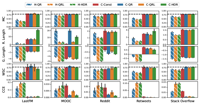
Figure 3: Performance of different methods producing a region for the time on real world datasets using the CLNM model. Heuristic methods are hatched.

The first row of the figure demonstrates that all CP methods attain the desired marginal coverage. In contrast, heuristic methods generally undercover, which aligns with expectations. The second row focuses on the average length of the prediction regions. Here, it is evident that heuristic methods generate smaller regions compared to their conformal counterparts. While this might seem beneficial, it is important to note that these smaller regions result from undercoverage, which diminishes their practical utility.

Among the heuristic methods, H-HDR consistently produces regions of smaller or equal lengths compared to H-QR and H-QRL for each prediction instance. Consequently, H-HDR emerges as the method with the smallest average region length. H-QR, not adjusting adequately to the right-skewed nature of the distributions, tends to yield larger regions.

Focusing now on the conformal methods, we exclude heuristic methods from this analysis due to their inability to achieve marginal coverage, which can lead to arbitrarily small regions. In the second row, the variations in average region length among CP methods differ across datasets. Notably, C-HDR, unlike its heuristic counterpart H-HDR, often yields larger average region lengths, especially in the LastFM, MOOC, and Retweets datasets. This difference arises because C-HDR adjusts the initial H-HDR prediction regions adaptively based on the individual predictive distributions. In contrast, C-QR and C-QRL modify their respective heuristic initial regions by a constant amount. While C-Const generates identical regions regardless of the history ${\bm{h}}$, it occasionally has the smallest average region length while still maintaining marginal coverage. This occurs because C-Const does not tailor its regions to account for extreme right-skewed distributions, leading to regions that are either slightly larger or significantly smaller compared to other conformal methods. These two phenomena are exemplified in a toy example shown in Fig. 4.

This figure demonstrates a scenario where the average region length of C-HDR is larger than that of other conformal methods in inter-arrival time prediction. The first row shows predictive distributions in blue and their corresponding realizations as dashed lines, based on three observations from a calibration dataset. In the second row, the prediction regions for seven methods are depicted with $\alpha=0.5$. All heuristic methods underperform, achieving a maximum coverage of only $1/3$, which is less than the desired coverage of 0.5. Conformal prediction methods, in response, adjust their prediction regions to achieve coverage in at least two out of three cases. Despite H-HDR always producing shorter or equivalent lengths compared to H-QR and H-QRL, C-HDR generates larger regions on average than other conformal methods. Again, C-Const, which does not adapt to individual predictive distributions, presents the smallest average regions among the conformal methods in this particular example. C-Const however does not achieve conditional coverage even asymptotically.

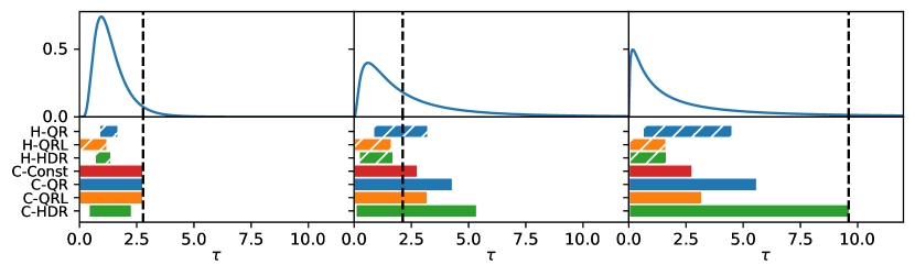
Figure 4: The figure showcases predictive distributions (blue) and realizations (dashed lines) in the first row, based on a calibration dataset. The second row illustrates prediction regions for various methods with $\alpha=0.5$. It highlights the undercoverage of heuristic methods, the adaptive adjustments of conformal methods, and the notable differences between C-HDR and other methods in terms of region size. We provide an additional example with $\alpha=0.2$ in Appendix C.

Returning to Figure 3, the third row introduces an alternative aggregation method for region lengths – the geometric mean. This method assigns less weight to larger regions and more to smaller ones. Here, C-HDR’s performance is more in line with other conformal methods, indicating that average region length might not be a reliable metric, particularly in cases of high variability in conditional distributions.

The fourth and fifth rows of the figure assess conditional coverage. WSC denotes coverage over the worst slab, with methods closer to $1-\alpha$ being preferable, whereas CCE represents a conditional coverage error, which should be minimized. Conformal methods, already proficient in achieving marginal coverage, exhibit a conditional coverage that is usually better than heuristic methods based on the evaluated metrics. Methods capable of tailoring prediction regions to specific instances are expected to exhibit enhanced conditional coverage. Although the WSC metric reveals no marked distinction among conformal methods, the CCE metric shows that C-HDR frequently attains one of the highest levels of conditional coverage. Moreover, C-QR often outperforms C-QRL in conditional coverage. As anticipated, the CCE metric reveals that C-Const generally exhibits the poorest conditional coverage, attributable to its lack of adaptability.

7.4.2 Prediction regions for the mark

Figure 5 presents similar metrics than in Figure 3, but focuses on methods that generate prediction sets exclusively for the mark. Here, the heuristic methods H-APS and H-RAPS already meet the marginal coverage criteria, meaning that conformal prediction primarily offers theoretical backing rather than significant changes in predictions.

Turning our attention to the conformal methods, these methods show similar region lengths across all datasets, with the exception of Reddit, where C-PROB exhibits smaller region lengths. However, on this same dataset and on Stack Overflow, C-PROB has a poor conditional coverage compared to both other conformal methods and heuristic methods. This reflects similar findings discussed in Section Section 7.4.1, where the method C-Const manages to attain short prediction regions, albeit with weak conditional coverage. This is explained due to the fact that, in contrast to C-APS, C-PROB does not achieve conditional coverage asymptotically.

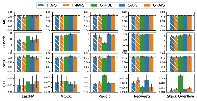
Figure 5: Performance of different methods producing a region for the mark on real world datasets using the CLNM model. Heuristic methods are hatched.

7.4.3 Joint prediction regions for the arrival time and the mark

Figure 7 displays the same metrics as Figures 3 and 5, but it specifically focuses on methods that generate bivariate prediction sets for both the arrival time and the mark. Recall that we consider two main approaches. The first combines individual prediction regions, as detailed in Section 6.1. Under this approach, we examine two variants: QRL-RAPS, which merges QRL for time with RAPS for the mark, and HDR-RAPS, which combines HDR for time with RAPS for the mark. The second approach, outlined in Section 6.2, directly creates a bivariate prediction region. Conformal versions of these methods are also considered in our analysis.

In the first row, we see that conformal methods successfully achieve marginal coverage, whereas heuristic methods tend to undercover. This observation mirrors the findings in the context of inter-arrival time prediction, as detailed in Section 7.4.1. The second row focuses on the average region length. Here, C-HDR-RAPS tends to produce larger regions on average compared to C-QRL-RAPS, consistent with the explanations provided in Section 7.4.1 and Fig. 4. Notably, C-HDR shows competitive average region lengths, outperforming C-HDR-RAPS. This highlights the benefit of creating joint regions that account for the interdependence between time and mark. In the third row, C-HDR stands out as the most effective on each dataset when using the geometric mean to average region lengths.

The last two rows illustrate that conformal methods attain better conditional coverage than their heuristic counterparts, echoing the results observed in Section 7.4.1. C-HDR obtains a competitive conditional coverage, especially on the dataset Reddit.

For illustration, Figure 6 gives examples of naive bivariate prediction regions generated by C-QRL-RAPS and C-HDR-RAPS, as well as a bivariate highest density region using C-HDR. We can see that the naive approaches produce constant size intervals for each of the marks selected by the C-RAPS approach. Conversely, C-HDR is able to generate variable-length prediction intervals for each mark by taking the inter-dependencies between the two variables into account.

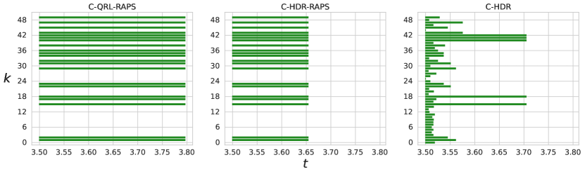
Figure 6: Examples of prediction regions generated by CLNM using the C-QRL-RAPS, C-HDR-RAPS, and C-HDR methods for the last event of a test sequence of the LastFM dataset.

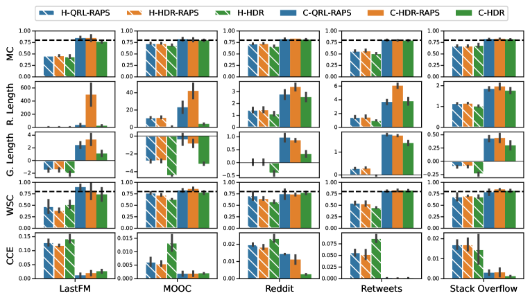
Figure 7: Performance of different methods producing a joint region for the time and mark on real world datasets using the CLNM model. Heuristic methods are hatched.

7.4.4 Empirical coverage for different coverage levels

Fig. 8 shows the marginal coverage achieved by various methods generating joint prediction regions for both the arrival time and mark. This figure extends the analysis beyond the specific miscoverage level of $\alpha=0.8$, as shown in the first row of Fig. 7, by including a range of coverage levels.

It is evident that heuristic methods generally underperform at all coverage levels, with this tendency becoming more pronounced at higher coverage levels. Conversely, conformal methods that construct individual predictions (outlined in Section Section 6.1) often overcover, particularly at lower coverage levels, due to their inherent conservativeness. Notably, C-HDR strikes an appropriate balance, maintaining the correct level of conservativeness across the various coverage levels.

In Appendix B, we provide additional results for the coverage per level in the context of prediction regions for the time or for the mark.

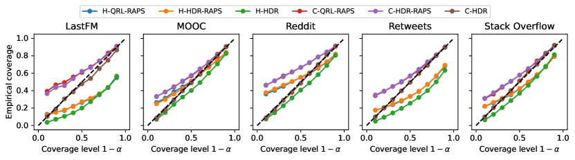
Figure 8: Empirical marginal coverage for different coverage levels with the CLNM model. All conformal methods achieve marginal coverage but the naive method tends to overcover, especially for small coverage levels. The heuristic methods do not achieve coverage in most cases.

8 Conclusion and future work

By integrating the methodologies of conformal prediction and neural TPPs, we have established a more robust approach to uncertainty quantification in TPPs. This is achieved by creating distribution-free joint prediction regions for the arrival time and its associated mark. The main challenge is to handle both a strictly positive, continuous response and a categorical response without distributional assumptions. We have also explored independently generating univariate prediction regions for the arrival time and the mark.

Our experiments highlight the importance of using conformal inference to ensure finite-sample marginal coverage. Indeed, heuristic methods tend to undercover in cases involving the prediction of arrival time or the simultaneous prediction of both arrival time and marks, with occasional success in predicting marks alone.

We also emphasize the significance of choosing appropriate conformal scores. C-HDR and C-QR show good conditional coverage, unlike C-Const, which lacks adaptability. The non-adaptive nature of C-Const leads to shorter average region lengths, which may appear advantageous at first glance. The same holds for C-PROB.

Our analysis underscores the importance of considering interdependence. Indeed, C-HDR, our extension of HPD-split [16] to bivariate outputs, outperforms C-HDR-RAPS. The superiority of C-HDR stems from its incorporation of joint regions that effectively consider and account for interdependence, whereas C-HDR-RAPS, in contrast, simplistically combines individual prediction regions through Bonferroni adjustments.

While this paper focuses on marked TPPs, the techniques presented here, especially those involving C-HDR, have the potential to extend to other prediction problems where the target variable is a vector comprising a combination of continuous and categorical variables. To the best of our knowledge, this is the first time such prediction regions are explored in the context of conformal prediction.

There are multiple possible directions for future work. First, we would like to relax the exchangeability assumption between sequences. Second, we want to explore conformal methods that specifically target an approximate notion of conditional coverage. Lastly, we aim to investigate sequence splitting techniques and the integration of block structures to effectively address serial dependence in a sequence.

Appendix A Results on other models

In Section 7.4, we provided results for the CLNM neural TPP model presented in Section 7.2. In Sections A.1, A.2 and A.3, we present additional findings for the FNN, RMTPP, and SAHP models, respectively. Across all these models, our conclusions align with those outlined in Section 7.4, applicable to all scenarios considered, namely, predictions for the time, the mark, or joint predictions on the time and mark.

A.1 FNN

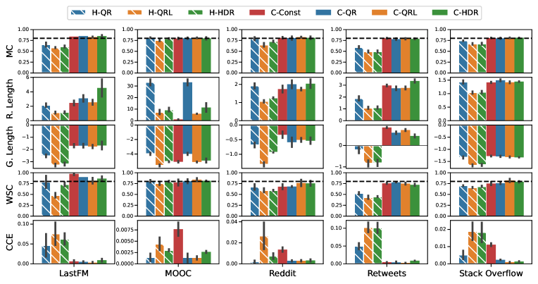
Figure 9: Performance of different methods producing a region for the time on real world datasets using the FNN model.

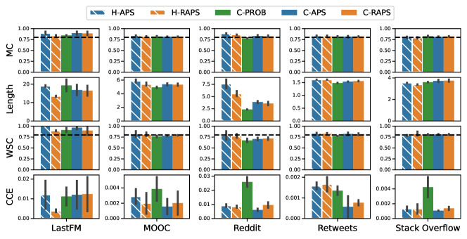
Figure 10: Performance of different methods producing a region for the mark on real world datasets using the FNN model.

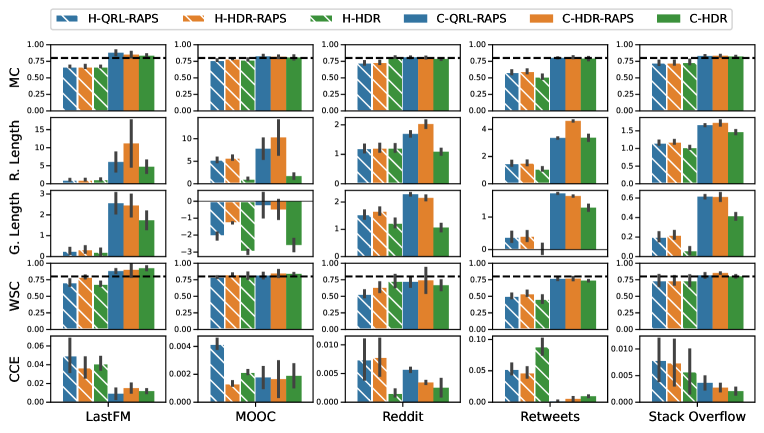
Figure 11: Performance of different methods producing a joint region for the time and mark on real world datasets using the FNN model.

A.2 RMTPP

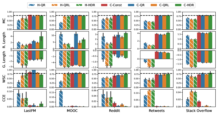
Figure 12: Performance of different methods producing a region for the time on real world datasets using the RMTPP model.

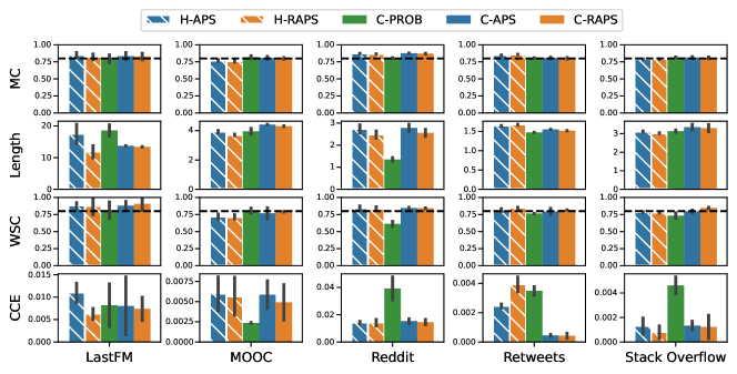
Figure 13: Performance of different methods producing a region for the mark on real world datasets using the RMTPP model.

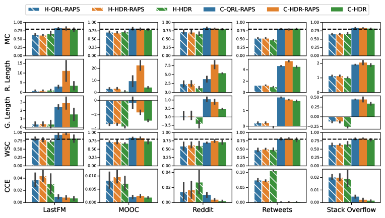
Figure 14: Performance of different methods producing a joint region for the time and mark on real world datasets using the RMTPP model.

Figure 15:

A.3 SAHP

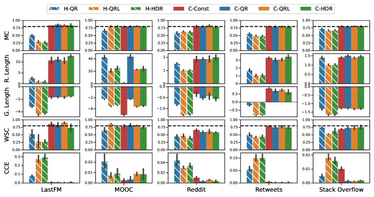
Figure 16: Performance of different methods producing a region for the time on real world datasets using the SAHP model.

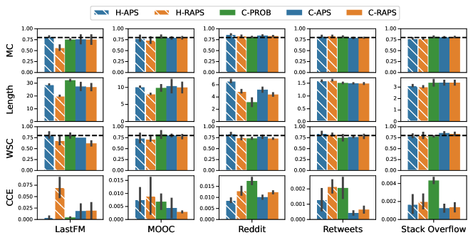
Figure 17: Performance of different methods producing a region for the mark on real world datasets using the SAHP model.

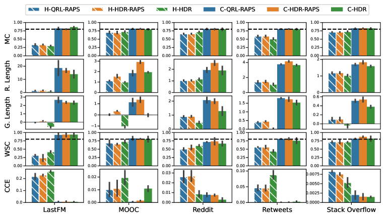
Figure 18: Performance of different methods producing a joint region for the time and mark on real world datasets using the SAHP model.

Appendix B Coverage per level

Section 7.4.4 discussed the empirical marginal coverage obtained at different coverage levels for methods that generate a joint prediction region on the arrival time and mark. In this section, we present additional results for methods that generate a prediction region individually for either the time or mark.

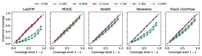
Figure 19: Empirical marginal coverage for different coverage levels for methods that produce a prediction region for the time with the CLNM model.

Fig. 19 shows that conformal methods for the time attain the desired coverage at all levels while heuristic methods generally undercover. This is expected and mirrors the observations in Section 7.4.4.

Fig. 20 shows that all methods, either heuristic or conformal, overcover for small coverage levels, while coverage is attained for high coverage levels. The reason is that all methods that generate a prediction set for the mark guarantee that prediction sets are not empty by always adding the class with the highest probability, as presented in Section 7.1. We do not observe overcoverage for high coverage levels because the class with highest probability will almost always be included. However, for low coverage levels, prediction sets that would normally be empty now include the mark with the highest probability, which leads to increased coverage.

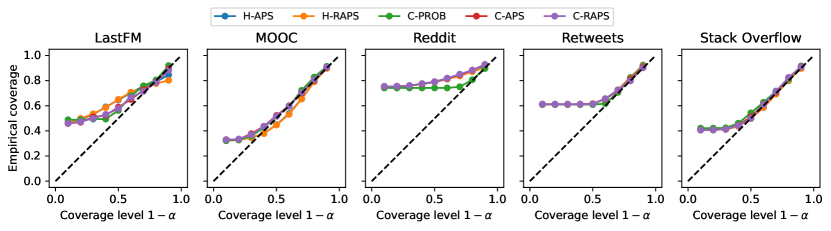
Figure 20: Empirical marginal coverage for different coverage levels for methods that produce a prediction region for the mark with the CLNM model.

Appendix C Additional example

In Fig. 4 in Section 7.4.1, we presented an example illustrating prediction regions for the time for seven methods with $\alpha=0.5$. For completeness, we provide an additional toy example with $\alpha=0.2$ and a calibration dataset of 6 data points in Fig. 21. As in Fig. 4, the heuristic methods undercover, achieving a maximum coverage of $4/6$, which is less than the desired coverage of $0.8$. Notably, H-QRL and H-HDR produce exactly the same prediction regions because the densities are decreasing in this case. Conformal methods adjust the predictions regions to achieve coverage in at least five out of six cases. Similarly to Fig. 4, C-HDR generates larger regions on average than other conformal methods despite H-HDR always producing shorter or equivalent lengths compared to H-QR and H-QRL.

Figure 21: Toy example with $\alpha=0.2$ and a calibration dataset of 6 data points.

Appendix D Partitioning for conditional coverage

In this section, we elaborate on the choice of distance function to create the partitions for the metric CCE introduced in Section 7.3. On Fig. 22, we show the CDF of $Z$ for all instances in the calibration dataset of the Reddit dataset. As shown in Fig. 22(a), instances where the distributions of $Z$ have the longest tails exhibit extreme distances from other distributions, resulting into their isolation into small clusters. Fig. 22(b) shows that, by instead focusing on the random variable $\log Z$, we achieve more balanced cluster sizes, which is crucial to have an accurate estimation of coverage within each partition.

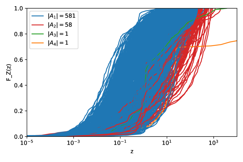
((a)) Partitions obtained with the distance $d_{Z}$.

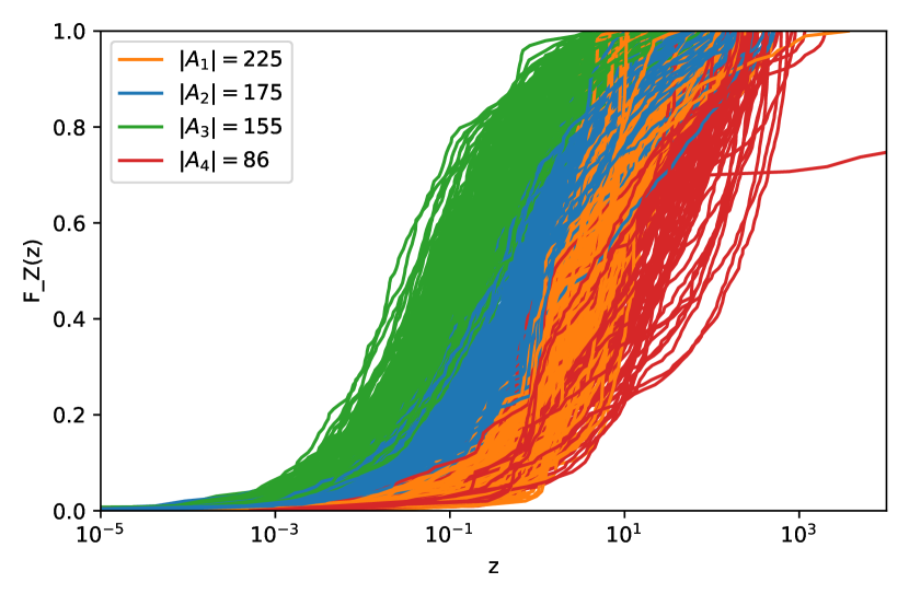
((b)) Partitions obtained with the distance $d_{\log Z}$.

Figure 22: The two subfigures show the CDF of $Z$ for all instances in the calibration dataset of the Reddit dataset. The colors determine the partition in which an instance falls according to the distance $d_{Z}$ on the left and $d_{\log Z}$ on the right, as introduced in Section 7.3. The legend denotes the size of each cluster of the partition.

Appendix E Additional examples of joint prediction regions

Figs. 23, 25, 24 and 26 present additional predictions regions generated by conformal methods on the datasets MOOC, Reddit, Retweets and Stack Overflow, respectively. We observe that C-HDR generally selects more marks than C-QRL-RAPS and C-HDR-RAPS. However, the joint region produced by C-HDR is usually smaller.

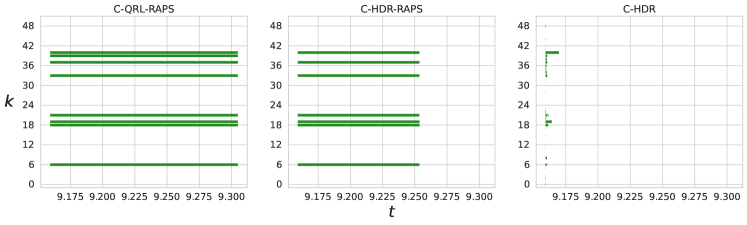
Figure 23: Example of joint prediction regions generated for the last event of a test sequence in the MOOC dataset.

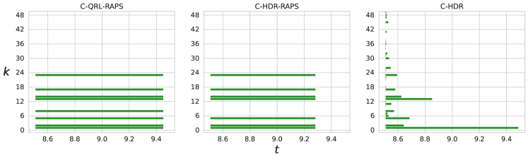
Figure 24: Example of joint prediction regions generated for the last event of a test sequence in the Reddit dataset.

Figure 25: Example of joint prediction regions generated for the last event of a test sequence in the Retweets dataset.

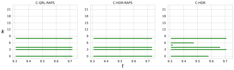
Figure 26: Example of joint prediction regions generated for the last event of a test sequence in the Stack Overflow dataset.

References

- \bibcommenthead
- [1] Enguehard, J., Busbridge, D., Bozson, A., Woodcock, C. & Hammerla, N. Y. Neural temporal point processes for modelling electronic health records (2020). ML4H.
- [2] Bacry, E. & Muzy, J. F. Hawkes model for price and trades high-frequency dynamics (2014). Quantitative Finance.
- [3] Farajtabar, M. et al. Coevolve: A joint point process model for information diffusion and network co-evolution (2015). Neurips.
- [4] Ogata, Y. Space-time point-process models for earthquake occurrences (1998). Annals of the Institute of Statistical Mathematics, 50(2):379–402.
- [5] Hawkes, A. G. Point spectra of some mutually exciting point processes (1971). Journal of the Royal Statistical Society: Series B, 33(3).
- [6] Mei, H. & Eisner, J. The neural hawkes process: A neurally self-modulating multivariate point process (2016). Neurips.
- [7] Shchur, O., Türkmen, A. C., Januschowski, T. & Günnemann, S. Neural temporal point processes: A review (2021). Proceedings of 13th Joint Conference on Artificial Intelligence.
- [8] Bosser, T. & Ben Taieb, S. On the predictive accuracy of neural temporal point process models for continuous-time event data (2023). TMLR.
- [9] Vovk, V., Gammerman, A. & Shafer, G. Algorithmic Learning in a Random World (Springer International Publishing, 2005). URL https://link.springer.com/book/10.1007/978-3-031-06649-8.
- [10] Candès, E. J., Lei, L. & Ren, Z. Conformalized survival analysis (2023). Journal of the Royal Statistical Society Series B: Statistical Methodology.
- [11] Gui, Y., Hore, R., Ren, Z. & Barber, R. F. Conformalized survival analysis with adaptive cutoffs (2023). Biometrika.
- [12] Stankeviciute, K., M. Alaa, A. & van der Schaar, M. Ranzato, M., Beygelzimer, A., Dauphin, Y., Liang, P. & Vaughan, J. W. (eds) Conformal time-series forecasting. (eds Ranzato, M., Beygelzimer, A., Dauphin, Y., Liang, P. & Vaughan, J. W.) Advances in Neural Information Processing Systems, Vol. 34, 6216–6228 (Curran Associates, Inc., 2021). URL https://proceedings.neurips.cc/paper_files/paper/2021/file/312f1ba2a72318edaaa995a67835fad5-Paper.pdf.
- [13] Feldman, S., Bates, S. & Romano, Y. Calibrated Multiple-Output quantile regression with representation learning. Journal of machine learning research: JMLR 24, 1–48 (2023). URL https://www.jmlr.org/papers/v24/21-1280.html.
- [14] Lei, J., Robins, J. & Wasserman, L. Distribution free prediction sets. Journal of the American Statistical Association 108, 278–287 (2013). URL http://dx.doi.org/10.1080/01621459.2012.751873.
- [15] Hyndman, R. J. Computing and graphing highest density regions. The American statistician 50, 120–126 (1996). URL http://www.jstor.org/stable/2684423.
- [16] Izbicki, R., Shimizu, G. & Stern, R. B. CD-split and HPD-split: Efficient conformal regions in high dimensions. Journal of machine learning research: JMLR 23, 1–32 (2022). URL https://www.jmlr.org/papers/v23/20-797.html.
- [17] Romano, Y., Patterson, E. & Candes, E. Conformalized quantile regression. Advances in neural information processing systems (2019). URL https://proceedings.neurips.cc/paper/2019/hash/5103c3584b063c431bd1268e9b5e76fb-Abstract.html.
- [18] Romano, Y., Sesia, M. & Candès, E. J. Classification with valid and adaptive coverage (2020). URL https://proceedings.neurips.cc/paper_files/paper/2020/file/244edd7e85dc81602b7615cd705545f5-Paper.pdf.
- [19] Angelopoulos, A., Bates, S., Malik, J. & Jordan, M. I. Uncertainty sets for image classifiers using conformal prediction (2022). 2009.14193.
- [20] Vovk, V. Conditional validity of inductive conformal predictors (2012). ACML.
- [21] Foygel Barber, R., Candès, E. J., Ramdas, A. & Tibshirani, R. J. The limits of distribution-free conditional predictive inference. Information and Inference: A Journal of the IMA 10, 455–482 (2021). URL https://academic.oup.com/imaiai/article-pdf/10/2/455/38549621/iaaa017.pdf.
- [22] Isham, V. & Westcott, M. A self-correcting point process. (1979). Stochastic Processes and Their Applications, 8(3):335–347.
- [23] Bacry, E., Jaisson, T. & Muzy, J.-F. Estimation of slowly decreasing hawkes kernels: Application to high frequency order book modelling (2015). Quantitative Finance.
- [24] Farajtabar, M. et al. Shaping social activity by incentivizing users (2014). Neurips.
- [25] Du, N., Wang, Y., He, N., Sun, J. & Song, L. Time-sensitive recommendation from recurrent user activities (2015). Neurips.
- [26] Du, N. et al. Recurrent marked temporal point processes: Embedding event history to vector (2016). SIGKDD.
- [27] Zuo, S., Jiang, H., Li, Z., Zhao, T. & Zha, H. Transformer hawkes process (2020). ICML.
- [28] Zhang, Q., Lipani, A., Kirnap, O. & Yilmaz, E. Self-attentive hawkes processes (2020). ICML.
- [29] Yang, C., Mei, H. & Eisner, J. Transformer embeddings of irregularly spaced events and their participants (2022). ICLR.
- [30] Omi, T., Ueda, N. & Aihara, K. Fully neural network based model for general temporal point processes (2019). Neurips.
- [31] Shchur, O., Biloš, M. & Günnemann, S. Intensity-free learning of temporal point processes (2020). ICLR.
- [32] Waghmare, G., Debnath, A., Asthana, S. & Malhotra, A. Modeling inter-dependence between time and mark in multivariate temporal point processes (2022). CIKM.
- [33] Bosser, T. & Taieb, S. B. Revisiting the mark conditional independence assumption in neural marked temporal point processes (2023). ESANN.
- [34] Li, S. et al. Learning temporal point processes via reinforcement learning (2020). Neurips.
- [35] Upadhyay, U., De, A. & Gomez-Rodriguez, M. Deep reinforcement learning of marked temporal point processes (2018). Neurips.
- [36] Guo, R., Li, J. & Liu, H. Initiator: Noise-contrastive estimation for marked temporal point process (2018). IJCAI.
- [37] Mei, H., Wan, T. & Eisner, J. Noise-contrastive estimation for multivariate point processes (2020). Neurips.
- [38] Xiao, S. et al. Wasserstein learning of deep generative point process models (2017). Neurips.
- [39] Xiao, S. et al. Learning conditional generative models for temporal point processes (2018). AAAI.
- [40] Boyd, A., Bamler, R., Mandt, S. & Smyth, P. User-dependent neural sequence models for continuous-time event data (2020). Neurips.
- [41] Ben Taieb, S. Learning quantile functions for temporal point processes with recurrent neural splines (2022). AISTATS.
- [42] Vovk, V., Gammerman, A. & Saunders, C. Machine-Learning applications of algorithmic randomness. International Conference on Machine Learning (1999). URL https://www.semanticscholar.org/paper/298a09325dce98155779f9640ccae8fa5ddca62d.
- [43] Angelopoulos, A. N. & Bates, S. A gentle introduction to conformal prediction and Distribution-Free uncertainty quantification (2021). URL http://arxiv.org/abs/2107.07511.
- [44] Shafer, G. & Vovk, V. A tutorial on conformal prediction. Journal of machine learning research: JMLR (2008). URL https://www.jmlr.org/papers/volume9/shafer08a/shafer08a.pdf.
- [45] Papadopoulos, H., Proedrou, K., Vovk, V. & Gammerman, A. Inductive confidence machines for regression 345–356 (2002).
- [46] Gibbs, I. & Candès, E. Adaptive conformal inference under distribution shift (2021). URL https://proceedings.neurips.cc/paper_files/paper/2021/file/0d441de75945e5acbc865406fc9a2559-Paper.pdf.
- [47] Zaffran, M., Feron, O., Goude, Y., Josse, J. & Dieuleveut, A. Chaudhuri, K. et al. (eds) Adaptive conformal predictions for time series. (eds Chaudhuri, K. et al.) Proceedings of the 39th International Conference on Machine Learning, Vol. 162 of Proceedings of Machine Learning Research, 25834–25866 (PMLR, 2022). URL https://proceedings.mlr.press/v162/zaffran22a.html.
- [48] Stankeviciute, K., M Alaa, A. & van der Schaar, M. Conformal time-series forecasting. Advances in neural information processing systems 34 (2021). URL https://proceedings.neurips.cc/paper/2021/file/312f1ba2a72318edaaa995a67835fad5-Paper.pdf.
- [49] Tibshirani, R. J., Barber, R. F., Candes, E. J. & Ramdas, A. Conformal prediction under covariate shift (2019). URL http://arxiv.org/abs/1904.06019.
- [50] Xu, C. & Xie, Y. Conformal prediction for time series. IEEE transactions on pattern analysis and machine intelligence 45, 11575–11587 (2023). URL http://dx.doi.org/10.1109/TPAMI.2023.3272339.
- [51] Sun, S. & Yu, R. Copula conformal prediction for multi-step time series forecasting (2022). URL http://arxiv.org/abs/2212.03281.
- [52] Daley, D. & Vere-Jones, D. An introduction to the theory of point processes volume ii: General theory and structure (2007).
- [53] Rasmussen, J. G. Lecture notes: Temporal point processes and the conditional intensity function (2018).
- [54] Brehmer, J. et al. Comparative evaluation of point process forecasts (2021).
- [55] Sesia, M. & Candès, E. J. A comparison of some conformal quantile regression methods. Stat 9, e261 (2020).
- [56] Sesia & Romano. Conformal prediction using conditional histograms. Advances in neural information processing systems (2021). URL https://proceedings.neurips.cc/paper/2021/hash/31b3b31a1c2f8a370206f111127c0dbd-Abstract.html.
- [57] Kumar, S., Zhang, X. & Leskovec, J. Predicting dynamic embedding trajectory in temporal interaction networks (2019). KDD.
- [58] Bacry, E., Bompaire, M., Deegan, P., Gaiffas, S. & Poulsen, S. V. tick: a python library for statistical learning, with an emphasis on hawkes processes and time-dependent models (2018). 18:1-5, Journal of Machine Learning Research.
- [59] Bosser, T. & Ben Taieb, S. On the predictive accuracy of neural temporal point process models for continuous-time event data. Transactions of Machine Learning Research (TMLR) (2023).
- [60] Hendrycks, D. & Gimpel, K. Gaussian error linear units (gelus) (2023).
- [61] Kingma, D. P. & Ba, J. Adam: A method for stochastic optimization (2014). ICLR.
- [62] Cauchois, M., Gupta, S. & Duchi, J. C. Knowing what you know: valid and validated confidence sets in multiclass and multilabel prediction. Journal of machine learning research: JMLR 22, 3681–3722 (2021). URL https://dl.acm.org/doi/abs/10.5555/3546258.3546339.