Skewed Pivot-Blend Modeling with Applications to Semicontinuous Outcomes

Abstract

Skewness is a common occurrence in statistical applications. In recent years, various distribution families have been proposed to model skewed data by introducing unequal scales based on the median or mode. However, we argue that the point at which unbalanced scales occur may be at any quantile and cannot be reparametrized as an ordinary shift parameter in the presence of skewness. In this paper, we introduce a novel skewed pivot-blend technique to create a skewed density family based on any continuous density, even those that are asymmetric and nonunimodal. Our framework enables the simultaneous estimation of scales, the pivotal point, and other location parameters, along with various extensions. We also introduce a skewed two-part model tailored for semicontinuous outcomes, which identifies relevant variables across the entire population and mitigates the additional skewness induced by commonly used transformations. Our theoretical analysis reveals the influence of skewness without assuming asymptotic conditions. Experiments on synthetic and real-life data demonstrate the excellent performance of the proposed method.

Keywords: semicontinuous outcomes; skewed data; two-piece densities; two-part models; variable selection; composite models.

1 Introduction

Statisticians frequently encounter skewed data in biomedical, econometric, environmental, and social research. Commonly used models, such as linear regression, least absolute deviations, and robust regression, presume symmetric errors and are prone to significant distortions when confronted with skewness. To mitigate the issue, many researchers prefer transforming the data beforehand, with logarithmic-type transformations being among the most popular choices. Alternatively, some researchers use modal regression (Lee,, 1989) or median-based methods, which are less sensitive to the assumption of symmetric errors. However, these approaches do not explicitly account for and describe skewness.

To comprehensively address this issue, adopting a “joint” modeling approach becomes essential and beneficial. This paper simultaneously estimates location, scale, and skewness parameters, thus avoiding the risk of either concealing true skewness (masking) or erroneously detecting spurious skewness (swamping). This risk is present when using a stepwise procedure, such as fitting a modal regression and then assessing skewness based on residuals (Boos,, 1987). Our primary aim is not only to accommodate skewness, as many papers do, but to explicitly capture and characterize its effects.

Various distributions have been proposed in the literature for modeling skewed data. Azzalini, (1985) proposed a skewed density family including the skewed normal density as an example. Fernández and Steel, (1998) proposed a two-piece skewed distribution family that sets the mode at zero, including the skewed Student and Laplace distributions for Bayesian quantile regression (Arellano-Valle et al.,, 2005; Yu and Moyeed,, 2001). Rubio and Steel, (2015) extended the family by use of two scale parameters and additional shape parameters. Kottas and Gelfand, (2001) described an alternative two-piece skewed distribution family that keeps the median at zero, but the resulting density is discontinuous. For a historical account of two-piece distributions, interested readers may consult Rubio and Steel, (2020).

The existing constructions rely on a symmetric and unimodal raw density, introducing asymmetric scales based on either the mode or the median of the raw density. However, in numerous real-life applications, these assumptions may not hold. Particularly, the point at which skewness is enforced, termed the “pivotal point” in this paper, could be situated at any position or quantile. Intriguingly, this pivotal point distinguishes itself from the commonly used shift parameter, as opposed to the prevailing assumption in the existing literature. To overcome these limitations, there is a demand for a novel skewed distribution family that offers flexibility, continuity, and adaptability to any pivotal point of interest.

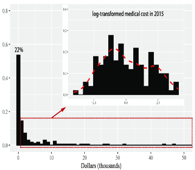
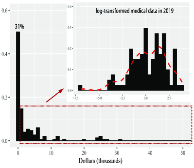
Figure 1: Some histograms of medical expenditures. Left: stratum ID 1098 (first PSU) of MEPS 2015, right: stratum ID 2109 (third PSU) of MEPS 2019. In each example, the main plot shows an excessive portion of zeros; the top right panel, excluding the zeros, plots the log-transformed positive values of response (with estimated density in red), which still exhibit asymmetry despite the transformation.

This study draws inspiration from the Medical Expenditure Panel Survey (MEPS) data, which is obtained from national surveys investigating the impact of various demographic variables on the medical expenses of patients in the United States. Notably, this dataset features a skewed response that includes a significant number of zeros, a phenomenon known as “semicontinuous outcomes” in the realms of economics and longitudinal studies (Olsen and Schafer,, 2001). To provide a visual representation, we employed two datasets (Agency for Healthcare Research and Quality,, 2015, 2019), as depicted in Figure 1, for illustration.

According to Figure 1, more than $20\%$ patients have zero medical expenditure, while the remaining exhibit highly skewed positive medical costs. Given that these zeros represent precisely zero medical expenses, rather than truncation, a two-part (or hurdle) model (Mullahy,, 1998) is a more appropriate choice than the Tobit model (Tobin,, 1958). In this approach, the binary part of the model captures zero-nonzero patterns, while the continuous part of the model addresses strictly positive outcomes. However, it is important to highlight that applying a standard log-normal two-part model may not yield sufficient power, owing to the asymmetry depicted in the upper-right panels of Figure 1. We have frequently observed that conventional transformations, such as logarithmic or power functions, not only fail to entirely eliminate skewness but also introduce nontrivial points around which asymmetric scales arise. Consequently, there may be a necessity to “reinforce” the transformed model to counteract the skewness effectively.

Another closely related challenge within the context of MEPS data analysis involves developing an interpretable two-part model. This entails the identification of a subset of medical cost-relevant predictors that apply to the entire population, serving as valuable guidance for policymakers. To the best of our knowledge, very few existing two-part models have considered the issue of joint variable selection, wherein each predictor can contribute to the response in a composite manner through the binary and continuous parts.

This paper attempts to address some aforementioned challenges for possibly skewed, semicontinuous outcomes. Our contributions are as follows.

1. We introduce a novel skewed pivotal-point adaptive family, designed to infuse skewness around an unknown pivotal point. The key “skewed pivot-blend” technique is versatile and can be applied to any raw density, regardless of its symmetry or unimodality. The resulting density remains continuous and accommodates many previous proposals.

2. We introduce the SPEUS framework (Skewed Pivot-Blend Estimation with Unsymmetric Scales) for simultaneous estimation of scales, pivotal point, and other location parameters. This framework offers useful variants, especially for modeling semicontinuous outcomes with joint variable selection. The resulting two-part method is capable of identifying relevant variables across the entire population and concurrently addressing the excessive skewness introduced by imperfect transformations

3. We conduct nonasymptotic analysis for sparse skewed two-part models, utilizing a notion of effective noise and Orlicz norms to derive sharp statistical error bounds in the presence of skewness and heavy tails. Our work quantifies how skewness and tail decay impact regularization parameters, prediction and estimation errors.

Notations and symbols.

Given two vectors $\alpha,\beta\in\mathbb{R}^{n}$, their inner product is $\langle\alpha,\beta\rangle=\alpha^{T}\beta$ and their elementwise product is denoted by the vector $\alpha\circ\beta$. Given a scalar function $l$ and a vector $a$, $l(a)=[l(a_{i})]^{n}_{i=1}$, i.e., $l$ is applied componentwise. Throughout the paper, we use $1_{A}(x)$ to denote the indicator function of $A$, taking 1 if $x\in A$ and 0 otherwise. In particular, given any vector $a\in\mathbb{R}^{n}$, define two indicator vectors $1_{+}(a)=\left[1_{a_{i}>0}\right]^{n}_{i=1},1_{-}(a)=\left[1_{a_{i}<0}\right]^{n}_{i=1}.$ Define $\mathbb{R}_{+}=[0,\infty)$. Given a continuous density $f$ (with respect to the Lebesgue measure $\mu$), we use $f(\cdot|A)$ to denote the conditional density given $A$, or $f(\cdot|A)=\frac{f(\cdot)}{\int_{A}f\,\mathrm{d}\mu}$. Given any matrix $A=[a_{1},\ldots,a_{p}]^{T}\in\mathbb{R}^{p\times m}$, its spectral norm and Frobenius norm are denoted by $\|A\|_{2}$ and $\|A\|_{F}$, respectively. The (2,1)-norm of $A$ is defined as $\|A\|_{2,1}=\sum^{p}_{j=1}\|a_{j}\|_{2}$. We use $A_{k}$ to denote the $k$th column of $A$. Given $a,b\in\mathbb{R}$, we use the shorthand notation $a\lor b$ ($a\land b$) to denote the maximum (minimum) of $a$ and $b$.

2 Skewed Pivotal-Blend Estimation

2.1 Skewed Pivot-Blend for Density Pasting

How to define a skewed distribution family from a unimodal, continuous, and symmetric density $\phi$ has attracted a lot of attention in the literature. Azzalini, (1985) multiplied $\phi$ by a perturbation function to define a so-called “skewed symmetric distribution” family, one well-known example being the skewed normal distribution. We refer the reader to Nadarajah and Kotz, (2003), Wang et al., (2004), and Azzalini, (2005) for variants and further extensions. On the other hand, the associated skewed distribution function often lacks an explicit form, and determining its mode can be a challenging task (Ma and Genton,, 2004).

“Two-piece” skewed distributions are popularly used in recent years. Fernández and Steel, (1998) introduced a two-piece transformation that rescales $\phi$’s negative and positive parts differently using an asymmetry parameter, allowing it to maintain the mode at zero. A reparametrization of the approach, following Arellano-Valle et al., (2005), includes the skewed Student and epsilon-skew-normal distributions (Fernández and Steel,, 1998; Mudholkar and Hutson,, 2000). Later, Rubio and Steel, (2015) extended this idea to include two scale parameters (and additional shape parameters). The motivation for our work largely stems from their two-piece form, even though it assumes that the median of $\phi$ is zero. Another two-piece distribution family due to Kottas and Gelfand, (2001) can guarantee a median at zero, but the resulting density is discontinuous, which may cause difficulties and instability in parameter estimation. Interested readers may refer to Jones, (2014) for a systematic framework of how to construct skewed distributions from a given symmetric density.

Despite the research in this area, two issues have caught our particular attention and deserve further investigation. Firstly, the majority of existing works stipulate that $\phi$ should be unimodal and symmetric. However, situations can arise where skewness manifests when dealing with non-unimodal data. There might also be a need for additional reinforcement to counteract skewness, even when employing an asymmetric density. Another more critical concern is that in previous works, the transition point at which unequal scales are imposed, referred to as the pivotal point in this paper, is typically set at the mode or the median. Nevertheless, skewness can persist when the density deviates from the assumptions above or below any quantile, a common occurrence when using an imperfect transformation.

In the following, we introduce a process known as “skewed pivot-blend” (or sometimes pivot-blend for brevity) to characterize skewness as a combination of both first-order and higher-order statistical effects. We define a versatile two-piece distribution framework with skewness, designed to (i) accommodate any asymmetric or non-unimodal $\phi$, (ii) model skewness associated with any pivotal point of interest, and (iii) maintain continuity. See Figure 2 for an illustration.

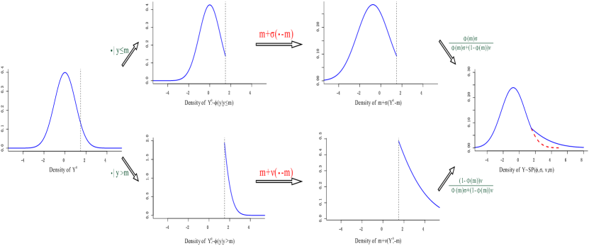
Figure 2: Diagram showing the process of “skewed pivot-blend” for constructing a skewed density: conditioning, affine transformations, and mixing. The two affine transformations ensure that the cut points remain fixed (alignment in the $x$-direction), and the mixing process guarantees the continuity of the resulting density (alignment in the $y$-direction).

We provide a step-by-step guide for constructing a new density function from an arbitrary continuous density (denoted as $\phi$), during which skewness is imposed around a pivotal point $m$ ($0<\Phi(m)<1$) and is defined by the left and right scales, $\sigma$ and $\nu>0$.

a) Pivotal-point conditioning: The density $\phi$ is conditioned into two separate densities, one for $y\leq m$, and the other for $y>m$, resulting in $\frac{\phi(y)1_{y\leq m}}{\Phi(m)}$ and $\frac{\phi(y)1_{y>m}}{1-\Phi(m)}$.

b) Affine transformation: Apply two separate affine transformations to the random variables associated with the aforementioned densities, concerning the pivotal point $m$: $m+\sigma(\cdot-m)$ and $m+\nu(\cdot-m)$. The resulting densities are $\frac{\phi\left(\frac{y-m}{\sigma}+m\right)1_{y\leq m}}{\Phi(m)\sigma}$ and $\frac{\phi\left(\frac{y-m}{\nu}+m\right)1_{y>m}}{(1-\Phi(m))\nu}$. It is crucial to emphasize that these transformations are not simple scalings, but are designed to ensure that the cut points of the density functions remain aligned.

c) Continuous mixing: Probability masses $p$ and $1-p$ are assigned to the two densities obtained from the last step, resulting in a new density function:

$$f(y)=p\times\frac{1}{\Phi(m)\sigma}\phi\big{(}\frac{y-m}{\sigma}+m\big{)}1_{y\leq m}+(1-p)\times\frac{1}{\{1-\Phi(m)\}\nu}\phi\big{(}\frac{y-m}{\nu}+m\big{)}1_{y>m},$$ (1)

where $\Phi$ denotes the distribution function of $\phi$ throughout the paper unless otherwise specified. Given that $\phi(m)>0$ typically holds, ensuring the continuity of $f$ at $m$ requires that ${p}/({\Phi(m)\sigma})=({1-p})/\{(1-\Phi(m)\nu\}$, which leads to a unique choice of $p$:

$$p=\frac{\Phi(m)\sigma}{\Phi(m)\sigma+\{1-\Phi(m)\}\nu},\mbox{ or }\ \ \frac{\mathbb{P}(Y\leq m)}{\mathbb{P}(Y>m)}=\frac{\Phi(m)\sigma}{\{1-\Phi(m)\}\nu}.$$ (2)

We sometimes refer to the process as the “forward” pivot-blend transform (to contrast with the “backward” pivot-blend transform to be introduced in Remark 2). When $\sigma=\nu$ or $m$ is not in the support of $\phi$, pivot-blend operates as a location-scale transformation. Otherwise, it serves as a versatile tool for modeling skewed data, encompassing various existing skewed density functions. Notably, the incorporation of a single pivotal point parameter $m$ substantially improves skewed data modeling in practical applications.

Definition 2.1 (Skewed pivot-blend (SP) family).

Given a continuous density $\phi$ and a pivotal point $m$, we say that $Y$ is a skewed random variable with $m$-associated left- and right-scale parameters $\sigma$ and $\nu$, i.e., $Y\sim\mbox{SP}^{(\phi)}(\sigma,\nu,m)$, if its density is given by

$$f(y;m,\sigma,\nu)=\frac{\phi\big{(}\frac{y-m}{\sigma}+m\big{)}1_{y\leq m}+\phi\big{(}\frac{y-m}{\nu}+m\big{)}1_{y>m}}{\Phi(m)\sigma+\{1-\Phi(m)\}\nu}.$$ (3)

We occasionally write $Y\sim\mbox{SP}^{(\phi)}$ and omit the parameters when there is no ambiguity. Throughout the paper, we use the term skewness to refer to asymmetric scales ($\sigma\neq\nu$), regardless of the shape of $\phi$.

The pivotal location $m$ can be translated to a pivotal quantile $q$. Let $q=\Phi(m)$, then an equivalent form of (3) is

$$\frac{\phi\big{(}\frac{y-\Phi^{-1}(q)}{\sigma}+\Phi^{-1}(q)\big{)}1_{\Phi(y)\leq q}+\phi\big{(}\frac{y-\Phi^{-1}(q)}{\nu}+\Phi^{-1}(q)\big{)}1_{\Phi(y)>q}}{q\sigma+(1-q)\nu}.$$

For the distribution function $F(y)=\frac{1}{\sigma\Phi(m)+\nu(1-\Phi(m))}\{\sigma\Phi(\frac{y-m}{\sigma}+m)1_{y\leq m}+[\nu\Phi(\frac{y-m}{\nu}+m)+(\sigma-\nu)\Phi(m)]1_{y>m}\}$, the new quantile at $m$ is related to the original quantile $q$ by $F(m)=\frac{q\sigma}{q\sigma+(1-q)\nu}\lessgtr q$ when $\sigma\lessgtr\nu$.

When working with the family described in Definition 2.1, it is a common practice to add a shift or intercept $\alpha\in\mathbb{R}$ and assume $Y-\alpha\sim\mbox{SP}^{(\phi)}(\sigma,\nu,m)$; however, it is crucial to note that $\alpha$ and $m$ are generally not redundant. This distinction arises because the operations of translation and asymmetric rescaling utilized in the skewed pivot-blend process do not commute (cf. Remark 1).

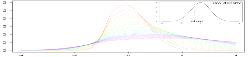
(a) $\phi\sim N(0,1)$, $m=\Phi^{-1}(0.25)$

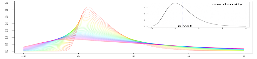
(b) $\phi$: Gumbel, $m$: mean

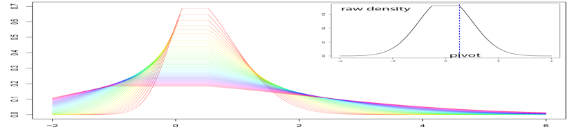
(c) $\phi$: flat modal, $m$: (rightmost) mode

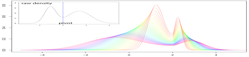
(d) $\phi\sim 0.4N(0.9,0.25)+0.6N(3.4,1),m=2$

Figure 3: Illustration of some SP families with varied $\sigma$ and $\nu$ (while maintaining a constant ratio). These plots demonstrate the versatility of skewed pivot-blend in generating a wide range of distributions for practical modeling, including asymmetry and diverse tails (which contrasts with traditional methods assuming symmetry in $\phi$ and median/mode in $m$).

Figure 3 provides visual examples of introducing skewness through pivot-blend around a nontrivial pivotal point, with variations in $\sigma$ and $\nu$ to demonstrate different tail decay behaviors.

Example 2.1 (Skewed double-gamma family).

Skewed densities may involve heavy tails and multimodality. When applied to the deneralized double-Gamma density (GDG), $p/\{2\gamma^{d}\Gamma(d/p)\}\allowbreak|y|^{d-1}\exp\{-|y|^{p}/\gamma^{p}\}$, an extension of Stacy, (1962), skewed pivot-blend reveals

SP^(GDG): $$\frac{p}{2[\Phi(m)\sigma+\{1-\Phi(m)\}\nu]\gamma^{d}\Gamma(d/p)}\Big{[}\big{|}\frac{y-m}{\sigma}+m\big{|}^{d-1}\exp\big{\{}-\frac{|(y-m)/\sigma+m|^{p}}{\gamma^{p}}\big{\}}1_{y\leq m}$$

$$\quad+\big{|}\frac{y-m}{\nu}+m\big{|}^{d-1}\exp\big{\{}-\frac{|(y-m)/\nu+m|^{p}}{\gamma^{p}}\big{\}}1_{y>m}\Big{]},$$

where $\gamma,d,p>0$ are parameters. The skewed GDG family comprises bimodal types such as the skewed double gamma ($p=1,m=0$) and skewed double Weibull ($d=p,m=0$). The unimodal skewed exponential power distribution family (Zhu and Zinde-Walsh,, 2009) is another instance ($\gamma=1$, $d=1$), including the skewed Laplace distribution and skewed normal distributions (Arellano-Valle et al.,, 2005; Mudholkar and Hutson,, 2000).

2.2 SPEUS for Skewed Regression

Skewed pivot-blend is a valuable tool for statistical modeling of a skewed outcome $y\in\mathbb{R}^{n}$ associated with $p$ predictors collected in the matrix $X\in\mathbb{R}^{n\times p}$. Given a density function $\phi$, if we assume

$$y-X\beta^{*}\sim\mbox{SP}^{(\phi)}(\sigma^{*},\nu^{*},m^{*})$$

and define $\rho=-\log\phi$, the estimation of $\beta^{*},\sigma^{*},\nu^{*},m^{*}$ can be formulated as a joint optimization problem

$$\begin{split}\min_{\beta,\sigma,\nu,m}\ &n\log\big{[}\sigma\Phi(m)+\nu\{1-\Phi(m)\}\big{]}+\sum^{n}_{i=1}\Big{\{}\rho\big{(}\frac{r_{i}-m}{\sigma}+m\big{)}1_{r_{i}-m\leq 0}\\ &+\rho\big{(}\frac{r_{i}-m}{\nu}+m\big{)}1_{r_{i}-m>0}\Big{\}},\quad\mbox{s.t.}\quad r=y-X\beta,\sigma>0,\nu>0,\end{split}$$ (4)

where the first term arises from the so-called “normalizing constant” which is a joint function of $m,\sigma,\nu$. Henceforth, we refer to the framework of (4) as the Skewed Pivot-blend Estimation with Unsymmetric Scales (SPEUS). We always assume that $\rho$ is constructed from a given density function unless otherwise specified. (4) is thus an instance of maximum likelihood estimation (MLE), and standard MLE asymptotic theory guarantees consistency and other properties. In practical implementation, the values of $r_{i}$ are rarely equal to $m$ and so conventional optimization algorithms like gradient descent, Newton’s method, and quasi-Newton methods can be readily applied. Given the nonconvex nature, initialization impacts estimates, especially for small sample sizes. We usually start location parameters at 0, but using a preliminary estimate like Yang et al., (2019) tends to yield better performance. A Bayesian approach can be developed as well. It is also worth pointing out that skewed pivot-blend, like other skewness-introducing methods, operates on a given density with asymmetric scales to handle skewed data. We do not explore nonparametric approaches in this paper (but refer to Appendix B for potential ideas involving kernels and data ranks).

Remark 1 (Pivotal Point vs. Intercept).

Typically, an intercept $\alpha$ is included the model, and so $r=y-X\beta=y-X^{\circ}\beta^{\circ}-1\alpha$, where $X=[1,X^{\circ}],X^{\circ}=[\tilde{x}_{1},\ldots,\tilde{x}_{n}]^{T},\beta=[\alpha,(\beta^{\circ})^{T}]^{T}$. Interestingly, when skewness is present, the pivotal point $m$ diverges from the intercept $\alpha$.

Specifically, based on previous discussions, we have the following density form

$$\sum_{i=1}^{n}\frac{\phi\big{(}\frac{y_{i}-\tilde{x}_{i}^{T}\beta^{\circ}-\alpha-m}{\sigma}+m\big{)}1_{y_{i}-\tilde{x}_{i}^{T}\beta^{\circ}\leq m+\alpha}+\phi\big{(}\frac{y_{i}-\tilde{x}_{i}^{T}\beta^{\circ}-\alpha-m}{\nu}+m\big{)}1_{y_{i}-\tilde{x}_{i}^{T}\beta^{\circ}>m+\alpha}}{\Phi(m)\sigma+\{1-\Phi(m)\}\nu}.$$

It is evident that $m$ plays a more intricate role compared to $\alpha$. If $\sigma=\nu$, the expression within the sum can be rewritten in a location-scale form: $(1/\sigma)\phi((y_{i}-\tilde{x}_{i}^{T}\beta^{\circ}-\alpha^{\prime})/\sigma)$, where $\alpha^{\prime}=\alpha+(1-\sigma)m$. In this special case, $m$ can be absorbed into the combined intercept $\alpha^{\prime}$, which is unique (ensuring the final model has no ambiguity). This also applies to $m\leq\min r_{i}$ or $m\geq\max r_{i}$, regardless of scale differences. However, in situations beyond the simple unskewed case (e.g., when $\sigma$ and $\nu$ are not exactly equal and $m$ is within the support of $r_{i}$ or $1/n<q<1-1/n$), $m$ cannot be incorporated into the intercept or casually discarded.

To the best of our knowledge, the distinct roles of pivotal point and intercept in the context of skewness have received little attention in existing literature. Our proposal is one of the first attempts to introduce pivotal point estimation into the statistical modeling of skewed data.

Remark 2 (Backward Pivot-blend for Residual Diagnostics).

Let’s start by rewriting the forward pivot-blend transform for generating a random variable following $\mbox{SP}^{(\phi)}(\sigma,\nu,m)$: With $Y^{0}_{-}\sim\phi(y\mid y\leq m),Y^{0}_{+}\sim\phi(y\mid y>m)$ and an independent Bernoulli variable $U\sim\mbox{Ber}(\sigma\Phi(m)/[\Phi(m)\sigma+\{1-\Phi(m)\}\nu])$, we can construct

$$\begin{split}Y=&\,\begin{cases}m+\sigma(Y^{0}_{-}-m)\mbox{ if }{U=1}\\ m+\nu(Y^{0}_{+}-m)\mbox{ if }{U=0},\end{cases}\end{split}$$

and guarantee that $Y$ follows $\mbox{SP}^{(\phi)}(\sigma,\nu,m)$. Conversely, given $f$ representing $\mbox{SP}^{(\phi)}(\sigma,\nu,m)$, we can use $Y_{-}\sim f(y\mid y\leq m)$, $Y_{+}\sim f(y\mid y>m)$ and an independent Bernoulli random variable $V\sim\mbox{Ber}(\Phi(m))$ to construct a random variable $Y^{0}\sim\phi$ using the “backward” pivot-blend:

$$Y^{0}=\Big{(}\frac{Y_{-}-m}{\sigma}+m\Big{)}1_{V=1}+\Big{(}\frac{Y_{+}-m}{\nu}+m\Big{)}1_{V=0}.$$ (5)

In addition to employing the inverse of the affine transformations in the forward process, the Bernoulli distribution here features a different probability. Thus, an $\mbox{SP}^{(\phi)}$ sample can be transformed into a weighted sample that follows $\phi$. Importantly, the functional form of the distribution $\Phi$ is not required to calculate the probability weights; instead, we can turn to the mixing probability formula (2)

$$\,\mathbb{P}(V=1)=\Phi(m)=\frac{\nu\,\mathbb{P}(Y\leq m)}{\nu\,\mathbb{P}(Y\leq m)+\sigma\,\mathbb{P}(Y>m)},\,\mathbb{P}(V=0)=\frac{\sigma\,\mathbb{P}(Y>m)}{\nu\,\mathbb{P}(Y\leq m)+\sigma\,\mathbb{P}(Y>m)}$$ (6)

and directly estimate these quantities from the data (also applicable to nonparametric skew estimation in Appendix B).

In the context of SPEUS, (5) can be used to generate “back-transformed” residuals for model diagnostics: once the parameters $\beta,\sigma,\nu,m$ are determined, a weighted sample can be created from the residual vector $r=y-X\beta$, which, if the model assumption holds, should adhere to $\phi$. First, define $\mathcal{L}=\{i:r_{i}\leq m\}$, $L=|\mathcal{L}|$, $\mathcal{R}=\{i:r_{i}>m\}$, and $R=|\mathcal{R}|$. As aforementioned, $\Phi(m)$ can be estimated by $L\nu/\{L\nu+R\sigma\}$. Next, define $\tilde{r}=[\tilde{r}_{i}]\in\mathbb{R}^{n}$:

$$\tilde{r}_{i}=\begin{cases}(\frac{r_{i}-m}{\sigma}+m)&\mbox{ if }{r_{i}\leq m}\\ (\frac{r_{i}-m}{\nu}+m)&\mbox{ if }{r_{i}>m,}\end{cases}\quad\mbox{ for }1\leq i\leq n.$$

Finally, assign two sets of nonuniform probabilities $p_{i}$ to $\tilde{r}_{i}$ based on (6):

$$p_{i}=\nu/(L\nu+R\sigma)\text{ for }i\in\mathcal{L},\text{ and }\sigma/(L\nu+R\sigma)\text{ for }i\in\mathcal{R}.$$

Now we can use the R software to plot a weighted histogram of $\tilde{r}_{i}$ and compare it to the hypothetical density $\phi$. This is akin to standard OLS diagnostics for checking the goodness-of-fit of residuals under the Gaussian assumption. In practical data analysis, after fitting the SPEUS model, one can display the back-transformed residual plot to verify if skewness has been adequately addressed (cf. Figure 4).

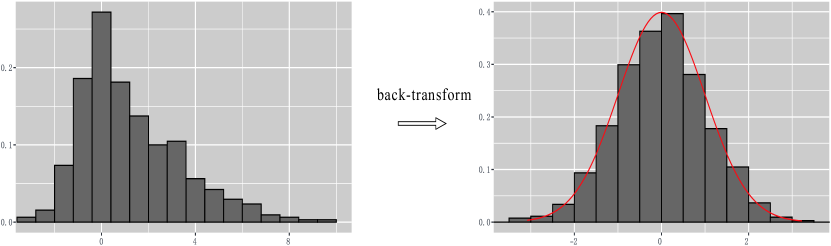
Figure 4: An illustration of the weighted histogram of back-transformed residuals. The left panel shows residuals from a skewed SP^(ϕ) model with a symmetric $\phi$, and the right panel displays backward pivot-blend residuals using estimated parameters. The model assumption is considered valid when the back-transformed residuals closely resemble $\phi$ (the red curve) and, importantly, exhibit symmetry, indicating effective handling of skewness.

2.3 Expansions of Skewed Pivot-Blend and Relevant Works

2.3.1 Extensions and Beyond

Our main focus is on applications where the loss function $\rho$ is derived from a single density function $\phi$. However, there are also variations of skewed pivot-blend that hold value across different applications and fields.

Skewed Pivot-blend for two densities.

Skewed pivot-blend extends capabilities to seamlessly “paste” two distinct densities with varying scales, while ensuring continuity at the pivotal point. Consider $\phi$ and $\psi$ as two continuous densities with respective distributions $\Phi$ and $\Psi$, and $m$ an interior point within the support of both densities. The process of conditioning, affine transformations, and mixing, using two scales, $\sigma$ and $\nu$ in relation to $m$, leads to

$$p\frac{\phi(\frac{y-m}{\sigma}+m)}{\Phi(m)\sigma}1_{y\leq m}+(1-p)\frac{\psi(\frac{y-m}{\nu}+m)}{(1-\Psi(m))\nu}1_{y>m}.$$ (7)

Choosing

$$p=\frac{\psi(m)\Phi(m)\sigma}{\phi(m)(1-\Psi(m))\nu+\psi(m)\Phi(m)\sigma}$$

results in the following continuous density:

$$\frac{\psi(m)\phi(\frac{y-m}{\sigma}+m)1_{y\leq m}+\phi(m)\psi(\frac{y-m}{\nu}+m)1_{y>m}}{\phi(m)(1-\Psi(m))\nu+\psi(m)\Phi(m)\sigma}.$$ (8)

This offers a means of fusing two distinct tail types with exceptional flexibility. Remarkably, even when $\sigma=\nu$, the pasted density in (8) does not conform to a location-scale form (in contrast to the single-density scenario, cf. Remark 1), and $m$ cannot be simply interpreted as a location shift. Beyond the estimation of scales, an intriguing question is to determine the pivotal point at which the two densities coalesce. Furthermore, the concept of skewed pivot-blend can be iteratively applied to paste multiple densities with varying scales. In multidimensional spaces, the pivotal point can be extended to a pivotal hyperplane for combining two densities, which is another intriguing topic for future exploration.

Skewed pivot-blend for bounded losses.

In our discussions, we generally assume that $\rho$ is a negative log-likelihood—for example, a convex $\rho$ function like Huber’s loss corresponds to a log-concave density. However, it is well established in robust statistics that bounded nonconvex losses are more effective in handling extreme outliers with high leverage. Two prominent examples are Tukey’s bisquare loss and Hampel’s three-part loss, both of which are bounded (or winsorized, preventing them from reaching $+\infty$) and are constructed using piecewise polynomials (Hampel et al.,, 2011). We can formulate a general objective for estimating the location parameters

$$\sum^{n}_{i=1}\big{\{}\rho(\frac{r_{i}-m}{\sigma}+m)1_{r_{i}\leq m}+\rho(\frac{r_{i}-m}{\nu}+m)1_{r_{i}>m}\big{\}}+n\chi_{0}\log\big{(}\frac{\sigma\Phi(m)/\{1-\Phi(m)\}+\nu}{1+\Phi(m)/\{1-\Phi(m)\}}\big{)}.$$ (9)

Here, $r=y-X\beta$, $0\leq\Phi(m)\leq 1$, and $\chi_{0}$ is for the purpose of calibration. The user can specify the particular forms of $\rho$ and $\Phi$ (and in the convex-$\rho$ case, $\Phi(m)$ may take $\lim_{M\to\infty}{\int^{m}_{-M}\exp(-\rho(t))\,\mathrm{d}t}/{\int^{M}_{-M}\exp(-\rho(t))\,\mathrm{d}t}$). In robust statistics, it is often recommended to first perform a separate ad-hoc robust scale estimation (Maronna et al.,, 2006), before proceeding to optimize (9) for the location parameters $\beta,m$. But various selections for $\sigma$ and $\nu$ influence the structure of the resulting asymmetric loss. This practice prompts a theoretical inquiry: is it possible to set a finite-sample error bound for location estimation using data-dependent scales, regardless of scale construction or the data distribution of $y$? For a nonasymptotic analysis using statistical learning theory, see Theorem A.1 for insights on how skewness adds to problem complexity and increases “excess risk”.

Finally, extensions of the skewed pivot-blend in nonparametric estimation, such as methods based on data ranks and kernels, can be found in Appendix B due to space constraints.

2.3.2 Other Related Works

Section 1 and Section 2.1 provide a list of relevant works on two-piece distributions. Moreover, as pointed out by a reviewer, our skewed pivot-blend idea shares similarities with the “composite models” in the fields of finance and actuarial sciences.

In such a context, researchers often aim to create a new size distribution by combining two distributions: one that is lighter-tailed on the left (e.g., lognormal or Weibull), and another that is heavier-tailed on the right (e.g., Pareto) (Cooray and Ananda,, 2005). This can be expressed as $p\cdot\frac{\phi(y)}{\Phi(m)}\cdot 1_{y\leq m}+(1-p)\cdot\frac{\psi(y)}{1-\Psi(m)}\cdot 1_{y>m}$ (Scollnik,, 2007), with the choice of $p$ to ensure the resulting density is smooth. An alternative proposal appeared in Bernardi and Bernardi, (2018), which, however, does not guarantee continuity. For further discussions on composite models, we refer to Klugman et al., (2012) and Dominicy and Sinner, (2017).

It is not difficult to see that the composite form described above corresponds to a specific instance of our skewed pivot-blend density (7) with $\sigma=1,\nu=1$. However, our research is driven by the need to tackle data skewness, where the values of $\sigma$ and $\nu$ are typically unknown and can vary. Our primary goal is to estimate these potentially distinct scales while also identifying the central pivotal point in the context of skew data analysis. (7) or (8) is notably different from the composite distribution even when $\sigma=\nu$ but not equal to 1.

Additionally, the composite model may be rigid and restrictive due to limited choices for the mixing parameter $p$ (Scollnik,, 2007). In contrast, Figure 3 illustrates the flexibility of SP distributions, taking on various shapes through adjustments in $\sigma$ and $\nu$. The versatility of the skewed pivot-blend, capturing both asymmetry and varied tail behaviors, offers a variety of distributions for practical modelingg.

3 Skewed Two-Part Model with Joint Sparsity

As mentioned in Section 1, our work is driven by the study of “semicontinuous outcomes” (Olsen and Schafer,, 2001), as defined by a significant proportion of values equaling 0, with the remaining values following a continuous, often skewed, distribution. For example, the MEPS datasets have many patients showing no medical expenditure (including the sum of out-of-pocket payment, insurance, Medicaid, Medicare, and other payments), and the rest with positive, highly skewed and heavy-tailed medical costs (see Figure 1). Semicontinuous outcomes are frequently encountered in biomedical and economic applications, as well as rainfall levels and daily drinking records (Hyndman and Grunwald,, 2000; Liu et al.,, 2008; Sarul and Sahin,, 2015).

Because zero medical cost means no medical service, rather than an outcome resulting from truncation or sampling, commonly used biometric models like the Tobit model and zero-inflated models (Tobin,, 1958; Lambert,, 1992) are not suitable. Instead, the two-part model (Cragg,, 1971; Mullahy,, 1998), sometimes also referred to as a hurdle model, is more appropriate. This model can be expressed as:

$$\mbox{\small Two parts for semicontinuous $y$:}\quad\begin{cases}\mathbb{P}(y_{i}=0)=\pi_{i}=1/\big{\{}1+\exp(-\tilde{x}^{T}_{i}b)\big{\}}\\ y_{i}\mid y_{i}>0\sim f(y_{i};\tilde{x}^{T}_{i}\beta).\end{cases}$$ (10)

In the binary part, the probability of observing a zero response is typically modeled using logistic regression or a probit model; in the continuous part, the density function $f$ represents a positive random variable with parameter $\tilde{x}_{i}^{T}\beta$. Without loss of generality, let’s assume that for $1\leq i\leq n$, $y_{i}>0$, while for $n<i\leq N$, $y_{i}=0$, and so the response and the overall prediction matrix $\widetilde{X}$ can be partitioned as

$$y=\big{[}[y_{1},\ldots,y_{n}]\,\,[0,\ldots,0]\big{]}^{T},\quad\widetilde{X}=\big{[}[\tilde{x}_{1},\dots,\tilde{x}_{n}]\,\,[\tilde{x}_{n+1},\dots,\tilde{x}_{N}]\big{]}^{T}=[X^{T}\,\,Z^{T}]^{T}.$$ (11)

We then derive the negative log-likelihood from the distribution defined in (10), with respect to a combination of the Lebesgue measure on $\mathbb{R}_{+}$ and a counting measure at 0:

$$-\sum^{N}_{i=1}\big{[}1_{y_{i}=0}\log\pi_{i}+1_{y_{i}>0}\log\{(1-\pi_{i})f(y_{i};\tilde{x}^{T}_{i}\beta)\}\big{]}$$

$$= \sum^{N}_{i=1}\big{[}-\tilde{x}^{T}_{i}b1_{y_{i}=0}+\log\big{\{}1+\exp(\tilde{x}^{T}_{i}b)\big{\}}\big{]}+\sum^{n}_{i=1}-\log f(y_{i};\tilde{x}^{T}_{i}\beta).$$ (12)

Each predictor makes a composite contribution to the response through two parts, but (3) is separable with respect to $b$ and $\beta$, making it amenable to optimization. Below, we will introduce two modifications to the classical two-part model to better address some challenges in modern applications: (a) mitigating skewness in the positive part through the use of pivot-blend, and (b) enhancing interpretability by incorporating joint variable selection across both model components.

First, specifying an ideal density function for the positive values of $y_{i}$ can be challenging. As a result, many researchers opt to employ a transformation $T(\cdot):(0,\infty)\rightarrow\mathbb{R}$, and assume that the transformed response $T(y_{i})$ ($1\leq i\leq n$) follows a symmetric distribution, such as a normal or a Laplace. With $\rho$ denoting the corresponding symmetric negative log-likelihood, the last term $\sum^{n}_{i=1}-\log f(y_{i};\tilde{x}^{T}_{i}\beta)$ in (3) now takes the form

$$\sum^{n}_{i=1}\rho({r_{i}})\quad\text{ with }r=T(y)-X\beta$$ (13)

where $r\in\mathbb{R}^{n}$ is the residual vector associated with the continuous component of the model. Nevertheless, asymmetry continues to manifest in the transformed data in various scenarios, as observed by Chai and Bailey, (2008). Our experience shows that routine transformations may not only fail to completely rectify skewness but also introduce a nontrivial pivotal point around which asymmetric scales arise. The technique detailed in Section 2 offers an effective remedy by replacing (13) with the following

$$\begin{split}&n\log[\sigma\Phi(m)+\nu\{1-\Phi(m)\}]+\sum^{n}_{i=1}\big{[}\rho\big{(}\frac{r_{i}-m}{\sigma}+m\big{)}1_{r_{i}\leq m}+\rho\big{(}\frac{r_{i}-m}{\nu}+m\big{)}1_{r_{i}>m}\big{]},\end{split}$$ (14)

where $\sigma,\nu,m$ are all unknown.

Second, practitioners of two-part models encounter another pressing challenge—the abundance of predictors collected. Variable selection provides a valuable tool for enhancing model interpretation and prediction, but in the context of two-part models, it is crucial to identify predictors that are relevant to the entire population, rather than just focusing on the subpopulation with positive responses or the subpopulation with zero responses. In other words, a predictor can only be eliminated if it bears zero coefficients in both the binary and continuous parts of the model.

Combining both elements, the incorporation of regularization and skewed pivot-blend allows us to formulate a sparse skewed 2-part $(\textbf{S}^{2})$ criterion for modeling semicontinuous outcomes with joint variable selection:

$$\begin{split}&\text{{S}${}^{2}$}:\min_{b,\beta,\sigma,\nu,m}n\log\big{[}\sigma\Phi(m)+\nu\{1-\Phi(m)\}\big{]}+\sum^{n}_{i=1}\big{\{}\rho\big{(}\frac{r_{i}-m}{\sigma}+m\big{)}1_{r_{i}-m\leq 0}\\ &\quad+\rho\big{(}\frac{r_{i}-m}{\nu}+m\big{)}1_{r_{i}-m>0}\big{\}}+\sum^{N}_{i=1}\big{[}-\tilde{x}^{T}_{i}b1_{y_{i}=0}+\log\big{\{}1+\exp(\tilde{x}^{T}_{i}b)\big{\}}\big{]}\\ &\quad+\lambda\|B\|_{2,1}+P_{2}(\sigma,\nu,m,\beta;\tau)\ \ \mbox{s.t.}\,\,\,r=T(y)-X\beta,B=[\sqrt{n}\beta,\sqrt{N}b],\sigma>0,\nu>0.\end{split}$$ (15)

Practically, it is common to include two intercepts, one for the binary part and one for the continuous part of the model, which are not subject to any penalty. The (2,1)-norm applied to matrix $B$ enforces the desired row-wise sparsity for joint variable selection, but can be substituted with a row-wise nonconvex penalty like group SCAD or MCP. Incorporating the scaling factors in the construction of $B$ is essential for the use of a single regularization parameter. The term $P_{2}$ represents an $\ell_{2}$-penalty, akin to ridge regression, to account for significant noise and design collinearity. An example is adding $(\tau/2)(1/\sigma^{2}+1/\nu^{2})$ (especially when $p\geq n$), which from a Bayesian perspective amounts to an inverse gamma prior on $\sigma^{2}$ and $\nu^{2}$. Empirical studies show that $\tau$ is not sensitive, and a small $\tau$ often suffices. Likewise, we suggest including an $\ell_{2}$-penalty on $m$ which translates to a Gaussian prior (or alternatively, a beta prior for the quantile parameter $q$), because in cases involving asymmetric scales $\sigma\neq\nu$, a moderate $|m|$ value (or $q$ near 1/2) can exert a considerable influence on the model, warranting deeper exploration in applications. (This might contrast with outlier effects which exhibit more of a tail behavior inconsistent with most data and are complex to model with a single distribution due to heterogeneity.) Adding the $\ell_{2}$ penalties also facilitates the theoretical analysis in the next section.

(15) involves the estimation of coefficients $b$, $\beta$, a pivotal point $m$, and two scales $\sigma,\nu$ and is one-sided directionally differentiable (She et al.,, 2021). In contrast to the conventional two-part (3), this criterion no longer shows separability in $(b,\beta)$ and includes a non-differentiable penalty. Efficient computation of the estimates can be achieved through optimization techniques. In handling the nondifferentiable (2,1)-penalty, we can express $\|B\|_{2,1}$ as $(1/2)\sum_{j=1}^{p}(B_{j,1}^{2}+B_{j,2}^{2})/a_{j}+a_{j}$ with each $a_{j}>0$. This yields a differentiable criterion, facilitating the use of standard optimization solvers such as Newton or quasi-Newton methods. Alternating optimization can also be used to improve scalability.

4 Analysis of Sparse Skewed Two Parts

In this section, we delve into the theoretical underpinnings of the sparse skewed two-part estimation (15) introduced earlier. Our investigation differs from classical asymptotics which assume a fixed number of predictors and an infinite sample size. Nonasymptotic theory remains relatively unexplored when considering the interplay of skewness, regularization, and heavy tails collectively. A significant challenge entails comprehending the impact of asymmetric scales, pivotal points, and sparsity on both statistical accuracy and the choice of the regularization parameter in finite sample sizes.

The key implications and contributions of our theoretical framework are as follows: (i) Applicability. Unlike conventional consistency studies, which frequently assume an i.i.d. data structure and require fixed $p$ with $n\rightarrow+\infty$, our theory is applicable to any values of $n$ and $p$, and does not require the design matrix to have i.i.d. rows. (ii) Effective Noise and Flexibility in Tails. Our investigation reveals that prediction and estimation errors, as well as the choice of the regularization parameter, are linked to the tail decay characteristics of the “effective noise”. The concept diverges from raw noise and often exhibits lighter tails (cf. Remark 3). Moreover, we employ Orlicz $\psi$-norms to model various tail behaviors (cf. Lemmas A.1–A.4), providing flexibility in real applications. In essence, when the effective noise shows light tails, implying a finite Orlicz norm with a “large” $\psi$ function, the presence of $\psi^{-1}$ in the choice of the regularization parameter leads to a reduced error bound (cf. (25) or (27)). (iii) Misspecification Tolerance. The core theorems do not require a zero-mean effective noise, as demonstrated in Theorems 1, 2, A.2, A.3, A.4. Consequently, our analysis applies to misspecified models (where the risk function associated with the given loss does not necessarily vanish at the statistical truth).

4.1 Preliminaries: Reparametrization and Effective Noise

Recall the loss function in (15), which can be represented by

$$\begin{split}l_{0}(\beta,b,m,\sigma,\nu)=&\sum^{n}_{i=1}\bigg{\{}\rho\big{(}\frac{r_{i}-m}{\sigma}+m\big{)}1_{r_{i}\leq m}+\rho\big{(}\frac{r_{i}-m}{\nu}+m\big{)}1_{r_{i}>m}\\ &+\log\big{[}\sigma\Phi(m)+\nu\{1-\Phi(m)\}\big{]}\bigg{\}}+\langle\mathfrak{L}(Zb;\mathpzc{Y}),1_{N}\rangle,\end{split}$$ (16)

where $r=y-X\beta$ denotes the plain residuals, $\rho$ and $\mathfrak{L}$ are two differentiable losses that respectively operate on the continuous part and binary part. Here, the observed data are represented by $y,\mathpzc{Y},X,Z$, with $y\in\mathbb{R}^{n}$, $X\in\mathbb{R}^{n\times p}$, $\mathpzc{Y}\in\{0,1\}^{N}$ and $Z\in\mathbb{R}^{N\times p}$ (cf. (11)). For simplicity, the section assumes that the number of rows in $X$ and $Z$ is each bounded by $cn$, with $n$ representing the order of the sample size and $c$ a positive constant.

To ease theory and presentation, we introduce some concatenated symbols. First, $\beta$ and $b$ can be combined into $\bar{\beta}$ as the coefficient vector for an extended design matrix $\bar{X}$:

$$\bar{\beta}=\mbox{vec}([\beta,b])=\begin{bmatrix}\beta\\ b\\ \end{bmatrix},\,\,\bar{X}=\begin{bmatrix}X&0\\ 0&Z\\ \end{bmatrix}.$$

We denote $[\beta_{k},b_{k}]^{T}$ by $\bar{\beta}_{k}$, the coefficients associated with the $k$th and $(p+k)$th columns of $\bar{X}$. Based on the problem structure in (16), we define

$$\bar{m}=m1_{n},\quad\varsigma=\begin{bmatrix}(1/\sigma)1_{n}\\ (1/\nu)1_{n}\\ \end{bmatrix},$$

where $1_{n}$ is to match the scale of the design matrices when considering prediction errors. Introduce $\zeta$ as the overall unknown vector, as well as $\gamma$ and $\mu$

$$\zeta=[\bar{\beta}^{T},\bar{m}^{T},\varsigma^{T}]^{T},\quad\gamma=[\bar{m}^{T},\varsigma^{T}]^{T},\quad\mu=[\bar{\eta}^{T},\bar{m}^{T},\varsigma^{T}]^{T},\quad\bar{\eta}=\bar{X}\bar{\beta}.$$ (17)

With the above notations, we can rewrite the general problem of interest as

$$l(\mu)+\|\varrho\bar{\beta}\|_{2,P}+\frac{\tau}{2}\|\gamma\|^{2}_{2},$$ (18)

where $l$ is the loss on $\mu$, $\|\bar{\beta}\|_{2,P}:=\sum^{p}_{k=1}P(\|\bar{\beta}_{k}\|_{2};\lambda)$ and $P$ is a sparsity-promoting penalty. Including $\varrho$ in the penalty allows for a scale adjustment based on the size of the designs, enabling a universal choice of $\lambda$ that is independent of the sample size in later theorems. In alternating optimization algorithms, $\varrho$ can takes $\kappa_{2,\infty}$ which represents the maximum column $\ell_{2}$-norm of $\bar{X}$, as a measure of the size of the design:

$$\kappa_{2,\infty}=\max_{1\leq k\leq 2p}\|\bar{X}_{k}\|_{2}=\max\big{\{}\|X_{1}\|_{2},\ldots,\|X_{p}\|_{2},\|Z_{1}\|_{2},\ldots,\|Z_{p}\|_{2}\big{\}}.$$

This quantity is typically on the order of $\sqrt{n}$. When $P$ is the $\ell_{1}$-penalty, (18) reduces to the previous $\textbf{S}^{2}$-criterion (15) for two-part models with skew and sparsity,

$$l(\mu)+\lambda\|\varrho\bar{\beta}\|_{2,1}+\frac{\tau}{2}\|\gamma\|^{2}_{2},$$ (19)

where $\|\bar{\beta}\|_{2,1}$ is short for $\sum^{p}_{k=1}\|\bar{\beta}_{k}\|_{2}$.

Next, we introduce the notion of “effective noise” to account for randomness, conditional on the design matrices $X,Z$. Given $l(\mu)$, define the effective noises associated with $\bar{\eta}^{*},\gamma^{*}$ as

$$\epsilon_{\bar{\eta}}=-\nabla_{\bar{\eta}}l(\mu)\big{|}_{\mu=\mu^{*}},\quad\epsilon_{\bar{m}}=-\nabla_{\bar{m}}l(\mu)\big{|}_{\mu=\mu^{*}},\quad\epsilon_{\varsigma}=-\nabla_{\varsigma}l(\mu)\big{|}_{\mu=\mu^{*}},$$ (20)

where $l$ is assumed to be differentiable at the statistical truth $\mu^{*}$.

When formulating statistical assumptions related to effective noises, it is important to account for different types of tail decay. We employ Orlicz $\psi$-norms, as well as some nonconvex variants capable of handling significantly heavier tails (cf. Appendix A.1). In the context of the Orlicz $\psi$-norm for a random variable (or vector) $X$, represented as $\|X\|_{\psi}$, $\psi(\cdot)$ is consistently assumed to be a nondecreasing, nonzero function defined on $\mathbb{R}_{+}$ with $\psi(0)=0$ (but not necessarily convex). For the Orlicz-norm of a random vector, please see (A.2). The inverse of $\psi$ is defined as $\psi^{-1}(x)=\sup\{t\in\mathbb{R}_{+}:\psi(t)\leq x\}$.

Some notable examples encompass the sub-Weibull $\psi_{q}$-norms, with $\psi$ defined as

$$\psi_{q}(x)=\exp(x^{q})-1,\ x\in\mathbb{R}_{+}$$ (21)

for $q>0$. (21) covers sub-Gaussian ($q=2$) and sub-Exponential ($q=1$) random variables, but as $q<1$, the sub-Weibull tails become much heavier (Götze et al.,, 2021). Another class is the $L_{q}$-norms, with $\psi(x)=x^{q}$ ($q\geq 1$). Orlicz norms provide a useful framework for analyzing skewed random variables (even when they lack a zero mean).

Remark 3 (Effective Noise vs. Raw Noise).

The effective noise, jointly determined by the data and the loss function, may differ from the plain “raw noise” defined by

$$\epsilon^{\mbox{\scriptsize{raw}}}:=y-\bar{m}^{*}-\eta^{*},$$ (22)

where $\eta^{*}=X\beta^{*}$. Comparing (20) with (22), one appealing aspect of $\epsilon_{\bar{\eta}}$ is that it tends to have light tails, even when $\epsilon^{\mbox{\scriptsize{raw}}}$ does not. Indeed, a straightforward derivative calculation based on (16) shows that

$$\,\epsilon_{\bar{\eta},i}=\begin{cases}\frac{\rho^{\prime}(\epsilon^{-}_{i})}{\sigma^{*}}1_{-}(\epsilon^{\mbox{\scriptsize{raw}}}_{i})+\frac{\rho^{\prime}(\epsilon^{+}_{i})}{\nu^{*}}1_{+}(\epsilon^{\mbox{\scriptsize{raw}}}_{i}),\quad 1\leq i\leq n,\\ \mathfrak{L}^{\prime}(Z^{T}_{i}b^{*};\mathpzc{Y}_{i}),\quad n<i\leq N,\end{cases}$$ (23a)

$$\,\epsilon_{\bar{m},i}=(\frac{1}{\sigma^{*}}-1)\rho^{\prime}(\epsilon^{-}_{i})1_{-}(\epsilon^{\mbox{\scriptsize{raw}}}_{i})+(\frac{1}{\nu^{*}}-1)\rho^{\prime}(\epsilon^{+}_{i})1_{+}(\epsilon^{\mbox{\scriptsize{raw}}}_{i})+\frac{\Phi^{\prime}(m^{*})(\nu^{*}-\sigma^{*})}{\sigma^{*}\Phi(m^{*})+\nu^{*}(1-\Phi(m^{*}))},$$ (23b)

$$\,\epsilon_{\varsigma,i}=\begin{cases}-\epsilon^{\mbox{\scriptsize{raw}}}_{i}\rho^{\prime}(\epsilon^{-}_{i})1_{-}(\epsilon^{\mbox{\scriptsize{raw}}}_{i})+\frac{\sigma^{*2}\Phi(m^{*})}{\sigma^{*}\Phi(m^{*})+\nu^{*}(1-\Phi(m^{*}))},\quad 1\leq i\leq n,\\ -\epsilon^{\mbox{\scriptsize{raw}}}_{i}\rho^{\prime}(\epsilon^{+}_{i})1_{+}(\epsilon^{\mbox{\scriptsize{raw}}}_{i})+\frac{\nu^{*2}\{1-\Phi(m^{*})\}}{\sigma^{*}\Phi(m^{*})+\nu^{*}(1-\Phi(m^{*}))},\quad n<i\leq 2n,\end{cases}$$ (23c)

where $\epsilon^{-}_{i}=\epsilon^{\mbox{\scriptsize{raw}}}_{i}/\sigma^{*}+m^{*},\epsilon^{+}_{i}=\epsilon^{\mbox{\scriptsize{raw}}}_{i}/\nu^{*}+m^{*}$. Therefore, if $|\rho^{\prime}|\leq M,|\mathfrak{L}^{\prime}|\leq B$ for some positive $M,B$ (e.g., when using Huber’s loss for $\rho$ and logistic deviance for $\mathfrak{L}$), then

$$\,\big{|}\epsilon_{\bar{\eta},i}\big{|}\leq\frac{M}{\sigma^{*}\land\nu^{*}}+B,$$ (24a)

$$\,\big{|}\epsilon_{\bar{m},i}\big{|}\leq\big{(}|1-\frac{1}{\sigma^{*}}|\lor|1-\frac{1}{\nu^{*}}|\big{)}M+\frac{|\sigma^{*}-\nu^{*}|}{\sigma^{*}\land\nu^{*}},$$ (24b)

$$\,\big{|}\epsilon_{\varsigma,i}\big{|}\lor\big{|}\epsilon_{\varsigma,i+n}\big{|}\leq M|\epsilon^{\mbox{\scriptsize{raw}}}_{i}|+(\sigma^{*}\lor\nu^{*}).$$ (24c)

It is evident that all components of $\epsilon_{\bar{\eta}}$ and $\epsilon_{\bar{m}}$ are bounded, thereby possessing a finite $\psi_{2}$-norm regardless of heavy tails that $\epsilon^{\mbox{\scriptsize{raw}}}$ may exhibit. Finally, it is worth noting that our theorems below impose Orlicz-norm conditions on the entire random vectors in (20), which is more flexible than assuming that the vectors have independent components, each with a finite Orlicz norm and a mean of 0 (cf. Lemma A.1). Furthermore, one can employ generalized Bernstein-Orlicz norms for random vector marginals, as described in Kuchibhotla and Chakrabortty, (2022) to develop sharper bounds under an additional minimum sample size constraint. We will not explore this further in the current paper.

4.2 Nonasymptotic Error Bounds

This part demonstrates some error bounds when using the $(2,1)$-penalty. Additional results can be found in the appendices, such as Theorem A.2 providing a universal form for $\lambda$ applicable to a broad range of tails, Theorem A.3 presenting an elementwise error bound, and Theorem A.4 examining a general sparsity-inducing penalty.

In what follows, we denote the group support of $\bar{\beta}$ as $\mathcal{J}(\bar{\beta})=\{k:\bar{\beta}_{k}=[\beta_{k},b_{k}]^{T}\neq 0,1\leq k\leq p\}$ and $J(\bar{\beta})$ is the cardinality of $\mathcal{J}(\bar{\beta})$. Also, define $\mathcal{J}^{*}=\mathcal{J}(\bar{\beta}^{*}),J^{*}=J(\bar{\beta}^{*})$, and $\hat{\mathcal{J}}=\mathcal{J}(\hat{\bar{\beta}})$ for short, and let $\mathcal{J}^{*C}\subset\{1,\ldots,p\}$ denote the complement of $\mathcal{J}^{*}$. The generalized Bregman function $\mathbf{\Delta}_{l}$ is useful in defining an appropriate error measure and making regularity conditions: given a function $l$ differentiable at $\eta^{\prime}$, $\mathbf{\Delta}_{l}(\eta,\eta^{\prime}):=l(\eta)-l(\eta^{\prime})-\left\langle\nabla l(\eta^{\prime}),\eta-\eta^{\prime}\right\rangle$ and $\bar{\mathbf{\Delta}}_{l}(\eta,\eta^{\prime}):=\{\mathbf{\Delta}_{l}(\eta,\eta^{\prime})+\mathbf{\Delta}_{l}(\eta^{\prime},\eta)\}/2$. The differentiability can be replaced by directional differentiability (She et al.,, 2021). If $l$ is also strictly convex, $\mathbf{\Delta}_{l}(\eta,\eta^{\prime})$ becomes the standard Bregman divergence $\mathrm{\mathbf{D}}_{l}(\eta,\eta^{\prime})$ (Bregman,, 1967). For the specific case of $l(\eta)=\|\eta-y\|_{2}^{2}/2$, $\mathbf{\Delta}_{l}(\eta,\eta^{\prime})=\|\eta-\eta^{\prime}\|_{2}^{2}/2$, or $\mathrm{\mathbf{D}}_{2}(\eta,\eta^{\prime})$ for short.

Theorem 1.

Assume that the effective noises $\epsilon_{\bar{\eta}},\epsilon_{\bar{m}}$, and $\epsilon_{\varsigma}$ are bounded in Orlicz norms: $\|\epsilon_{\bar{\eta}}\|_{\psi}\leq\omega_{\bar{\eta}},\|\epsilon_{\bar{m}}\|_{\psi}\leq\omega_{\bar{m}}$, and $\|\epsilon_{\varsigma}\|_{\varphi}\leq\omega_{\varsigma}$, where $\psi,\varphi$ satisfy: i) $\psi(x)$ is convex and $\psi(x)\psi(y)\leq c_{1}\psi(c_{0}xy)$, $\forall x,y\geq c_{2}$, for some positive $c_{0},c_{1},c_{2}$ (dependent on $\psi$ only), (ii) $\{\psi^{-1}(t)\}^{2}$ is concave or $\{\psi^{-1}(t)\}^{2}\lesssim t$ on $\mathbb{R}_{+}$; iii) $\{\varphi^{-1}(t)\}^{2}$ is concave or $\{\varphi^{-1}(t)\}^{2}\lesssim t$ on $\mathbb{R}_{+}$. Consider the estimator $\hat{\zeta}=[\hat{\bar{\beta}}^{\,T},\hat{\gamma}^{\,T}]^{T}$ by minimizing (19) with $\varrho\geq\kappa_{2,\infty}$ and $\lambda=A\big{\|}\bar{X}^{T}\epsilon_{\bar{\eta}}\big{\|}_{\infty}/\varrho$, where $A$ a large enough constant. Then

$$\mathbb{E}\Big{\{}\mathbf{\Delta}_{l}(\hat{\mu},\mu^{*})\vee{\tau}\mathrm{\mathbf{D}}_{2}(\hat{\gamma},\gamma^{*})\Big{\}}\,\lesssim\ c_{\psi}\omega_{\bar{\eta}}\,\varrho\,\psi^{-1}(p)\|\bar{\beta}^{*}\|_{2,1}+\frac{1}{\tau}\{\psi^{-1}(1)\}^{2}\omega^{2}_{\bar{m}}+\frac{1}{\tau}\{\varphi^{-1}(1)\}^{2}\omega_{\varsigma}^{2}+\tau\|\gamma^{*}\|_{2}^{2}.$$ (25)

where $c_{\psi}=c_{0}(1\vee c_{1}\vee 2\psi(c_{2}))^{2}\psi^{-1}(1)$.

Theorem 1 provides a bound on prediction and estimator errors, measured using generalized Bregman functions. Notably, this bound does not necessitate any regularity conditions on the design matrices or signal strength.

The assumptions (i)–(iii) on effective noise tails are mild, and the functions $\varphi$ and $\psi$ can be applied to a wide range of cases. For example, it is straightforward to verify that $\|\cdot\|_{\psi}$ can represent a $\psi_{q}$-norm with $q\geq 1$ (van der Vaart and Wellner,, 2013) where we can take $c_{1}=1,c_{2}=1,c_{0}=2^{1/q}$; $\|\cdot\|_{\varphi}$ can be sub-Weibull for some $q>0$, or an $L_{q}$-norm ($q\geq 2$) with heavy polynomial tails.

The first term on the right-hand side of (25), $c_{\psi}\omega_{\bar{\eta}}\,\varrho\,\psi^{-1}(p)\big{\|}\bar{\beta}^{*}\big{\|}_{2,1}$, is the dominant term scaling with $p$. Remark 3 emphasizes that $\epsilon_{\bar{\eta}}$ can have considerably lighter tails, enabling the choice of a large $\psi$ function. For instance, when $|\rho^{\prime}|\leq M,|\mathfrak{L}^{\prime}|\leq B$, we can take $\psi=\psi_{2}$, $\omega_{\bar{\eta}}=c\{M/(\sigma^{*}\land\nu^{*})+B\}$. Such a substantial $\psi$ function ensures that the error rate, which incorporates $\psi^{-1}$, stays well controlled, even when the raw noise (22) exhibits heavy tails.

Furthermore, with proper regularity conditions, another error bound that depends on $\bar{\beta}^{*}$ though its support $J^{*}$ can be derived.

Theorem 2.

Assume that the tails of effective noises are bounded in Orlicz norms: $\|\epsilon_{\varsigma}\|_{\varphi}\leq\omega_{\varsigma}$, $\|\epsilon_{\bar{\eta}}\|_{\psi_{q}}\leq\omega_{\bar{\eta}},\|\epsilon_{\bar{m}}\|_{\psi_{q}}\leq\omega_{\bar{m}}$ for some $q>0$. Let $\hat{\zeta}$ denote the optimal solution for (19) with $\varrho\geq\kappa_{2,\infty}$ and

$$\lambda=A\omega_{\bar{\eta}}(\log p)^{\frac{1}{q}}$$

for some large enough $A>0$. Suppose that there exist a large $K>0$ and a constant $\vartheta$ such that for any $\bar{\beta},\gamma$

$$(1+\vartheta)\lambda\varrho\big{\|}(\bar{\beta}-\bar{\beta}^{*})_{\mathcal{J}^{*}}\big{\|}_{2,1}\leq\mathbf{\Delta}_{l}(\mu,\mu^{*})+\lambda\varrho\big{\|}(\bar{\beta}-\bar{\beta}^{*})_{\mathcal{J}^{*C}}\big{\|}_{2,1}+K\lambda^{2}J^{*}.$$ (26)

Then

$$\mathbf{\Delta}_{l}(\hat{\mu},\mu^{*})\vee{\tau}\mathrm{\mathbf{D}}_{2}(\gamma,\gamma^{*})\lesssim KA^{2}\omega^{2}_{\bar{\eta}}(\log p)^{\frac{2}{q}}J^{*}+A^{2}\frac{\omega^{2}_{\bar{m}}}{\tau}(\log p)^{\frac{2}{q}}+\frac{\omega^{2}_{\varsigma}}{\tau}\{\varphi^{-1}(p^{A^{q}})\}^{2}+\tau\|\gamma^{*}\|_{2}^{2}$$ (27)

holds with probability at least $1-Cp^{-cA^{q}}$, where $C,c$ are positive constants.

To obtain a sufficient condition for the regularity condition (26), we can confine $\xi=\bar{\beta}-\bar{\beta}^{*}$ within a cone: $(1+\vartheta)\|\xi_{\mathcal{J}^{*}}\|_{2,1}\geq\|\xi_{\mathcal{J}^{C*}}\|_{2,1}$, and require either $\varrho^{2}\|\xi_{\mathcal{J}^{*}}\|^{2}_{2,1}\leq\tilde{K}J^{*}\mathbf{\Delta}_{l}(\mu,\mu^{*})$ or $\varrho^{2}\|\xi_{\mathcal{J}^{*}}\|^{2}_{2}\leq\tilde{K}\mathbf{\Delta}_{l}(\mu,\mu^{*})$ for some large $\tilde{K}>0$. These conditions extend the compatibility and restricted eigenvalue conditions which are widely used in sparse regression (Bickel et al.,, 2009; van de Geer and Bühlmann,, 2009). But (26) is less technically demanding.

In proving the theorem, we establish a more general result where $\psi_{q}$ can be replaced with a general $\psi$ and the appropriate choice for $\lambda$ is of the order $\omega_{\bar{\eta}}\psi^{-1}\left(p\psi{A\psi^{-1}(p)}\right).$ For more, please refer to Appendix A.4.

To illustrate the bound (27), let’s consider a scenario where $|\rho^{\prime}|\vee|\mathfrak{L}^{\prime}|\leq M$ for some $M>0$. Under the assumptions of independent centered effective noise components and $\|\epsilon^{\mbox{\scriptsize{raw}}}_{i}\|_{\psi_{q}}\leq\omega$ for some $q\in(0,2]$, we can deduce based on (24) in Remark 3 that the error bound in (27) is of the following order (treating $K,A$ as constants):

$$\begin{split}&\log p\cdot\Big{[}\big{(}1\vee\frac{1}{\sigma^{*2}}\vee\frac{1}{\nu^{*2}}\big{)}M^{2}J^{*}+\frac{1}{\tau}\big{\{}[(1-\frac{1}{\sigma^{*}})^{2}\lor(1-\frac{1}{\nu^{*}})^{2}]M^{2}+\big{(}\frac{\sigma^{*}\lor\nu^{*}}{\sigma^{*}\land\nu^{*}}-1\big{)}^{2}\big{\}}\Big{]}\\ &\quad+(\log p)^{2/q}\cdot\frac{1}{\tau}\{M\omega+\sigma^{*}\lor\nu^{*}\}^{2}+\tau\|\gamma^{*}\|_{2}^{2}.\end{split}$$

The bound varies with the number of predictors logarithmically, and quantifies the impact of asymmetric scales in the context of sparse skewed two-part models.

Remark 4.

Under suitable regularity conditions similar to those in Theorem 2, the following $(2,\infty)$-norm bound holds (cf. Theorem A.3 in Appendix A.5):

$$\|\hat{\bar{\beta}}-\bar{\beta}^{*}\|_{2,\infty}\leq C\frac{\sqrt{K\alpha}\lor\vartheta}{\alpha\sqrt{n}}A\Big{\{}\omega_{\bar{\eta}}+\frac{\omega_{\bar{m}}+\omega_{\varsigma}}{\sqrt{J^{*}}}\Big{\}}(\log p)^{\frac{1}{q}}$$ (28)

with probability at least $1-Cp^{-(A\vartheta)^{q}}-1/\varphi(cA\vartheta(\log p)^{{1}/{q}})$, where $C,c$ are positive constants and $A,K,\alpha,\vartheta$ can often be treated as constants. Hence with a proper signal strength $\min_{k\in\mathcal{J}(\bar{\beta}^{*})}\|\bar{\beta}_{k}^{*}\|_{2}>2CA(\sqrt{K\alpha}\lor\vartheta)\big{\{}\omega_{\bar{\eta}}+(\omega_{\bar{m}}+\omega_{\varsigma})/\sqrt{J^{*}}\big{\}}(\log p)^{\frac{1}{q}}/(\alpha\sqrt{n})$, (28) guarantees faithful variable selection, $\mathcal{J}^{*}\subset\hat{\mathcal{J}}$, with high probability.

Finally, our analysis can be extended to a general $P$ beyond the $\ell_{1}$-type penalty. See Appendix A.6 for more details.

5 Experiments

We conducted a variety of synthetic and real data experiments to evaluate the performance of the proposed method. Due to limited space, we only present a selection of our data analyses in the following subsections. Interested readers may refer to Appendix C for more experiment results.

5.1 Simulations

In this part, we conduct simulation experiments to compare our proposed methods with some popularly used approaches for skewed estimation. The predictor matrix $X=[X_{1},\ldots,X_{n}]^{T}\in\mathbb{R}^{n\times p}$ is generated by $X_{i}\overset{i.i.d.}{\sim}N(0,\Sigma)$, where $\Sigma=[\kappa^{|i-j|}]$ has a Toeplitz structure. The response vector is generated according to $y=X\beta^{*}+1\alpha^{*}+\epsilon$, where $\epsilon_{i}\overset{i.i.d.}{\sim}\mbox{SP}^{(\phi)}(\sigma^{*},\nu^{*},m^{*})$. In the setups to be introduced, we set $\alpha^{*}=0$ and $\beta^{*}=[12,13,14]^{T}$. The pivotal point will be chosen as the mean, median, mode, quartiles, and more.

The following methods are included for comparison: quantile regression (QR) (Koenker and Bassett Jr,, 1978), Bayesian quantile regression (BQR) (Yu and Moyeed,, 2001), $Z$-estimation quantile regression (ZQR) (Bera et al.,, 2016), adaptive M-estimation (AME) (Yang et al.,, 2019), epsilon-skew-normal regression (ESN) (Mudholkar and Hutson,, 2000), in addition to SPEUS. The first two methods require the user to specify a quantile parameter (Koenker,, 2009; Benoit and Van den Poel,, 2017); we employ the oracle quantile ($\Phi(m^{*})\sigma^{*}/[\Phi(m^{*})\sigma^{*}+\{1-\Phi(m^{*})\nu^{*}\}]$ (computed using the truth) in all experiments, and so denote the methods by QR^∗ and BQR^∗, respectively. In BQR^∗, the posterior mean estimate is obtained with 4000 MCMC draws after 1000 burn-in samples. For SPEUS, the scale parameters $\sigma$ and $\nu$, as well as the pivotal point $m$, are all considered unknown and are estimated from the data. Given each setup, we repeat the experiment for 50 times and evaluate the performance of each method based on $\mbox{Err}(\beta)$, Err($\sigma$) and Err($\nu$). $\mbox{Err}(\beta)$ is the (absolute) root-mean-square error on $\beta$, and Err($\sigma$) and Err($\nu$) denote the (relative) root-mean-square errors on $\sigma$ and $\nu$, i.e., $\mbox{Err}(\sigma)=\{\sum^{N}_{t=1}(\hat{\sigma}_{t}/\sigma^{*}-1)^{2}/N\}^{1/2}$, where $\hat{\sigma}_{t}$ is the estimate on the $t$th simulation dataset.

Ex 1. (Skewed Gaussian and skewed Laplace, $m^{*}=0$): Let $\phi$ be the standard normal or Laplace density, $n=300$, $\kappa=0.5$, $\sigma^{*}=0.2$ and $\nu^{*}=0.4,0.6,1.2$.

Ex 2. (Skewed Gaussian and skewed Laplace, $m^{*}\neq 0$): Let $\phi$ be the standard normal or Laplace density, $n=300$, $\kappa=0.2$, $m^{*}=\Phi^{-1}(0.75)$ (third quartile), $\sigma^{*}=0.3$ and $\nu^{*}=0.5,0.7,0.9$. (We also tried $m=\Phi^{-1}(0.25)$ but the results are similar and omitted.)

Skewed Gaussian
		$\nu^{*}/\sigma^{*}=2$				$\nu^{*}/\sigma^{*}=3$				$\nu^{*}/\sigma^{*}=6$
		Err($\beta$)	Err($\sigma$)	Err($\nu$)		Err($\beta$)	Err($\sigma$)	Err($\nu$)		Err($\beta$)	Err($\sigma$)	Err($\nu$)
QR∗		0.05	—	—		0.06	—	—		0.08	—	—
BQR∗		0.04	0.20	0.20		0.05	0.20	0.20		0.07	0.20	0.20
AME		0.04	0.44	0.44		0.04	0.44	0.44		0.06	0.44	0.44
ESN		0.04	0.42	0.42		0.04	0.42	0.42		0.06	0.42	0.42
SPEUS		0.04	0.13	0.08		0.05	0.18	0.06		0.06	0.29	0.05
Skewed Laplace
		$\nu^{*}/\sigma^{*}=2$				$\nu^{*}/\sigma^{*}=3$				$\nu^{*}/\sigma^{*}=6$
		Err($\beta$)	Err($\sigma$)	Err($\nu$)		Err($\beta$)	Err($\sigma$)	Err($\nu$)		Err($\beta$)	Err($\sigma$)	Err($\nu$)
QR∗		0.04	—	—		0.05	—	—		0.17	—	—
BQR∗		0.04	0.05	0.05		0.05	0.05	0.05		0.17	0.06	0.06
AME		0.04	0.23	0.20		0.05	0.25	0.21		0.17	0.24	0.20
ZQR		0.04	0.08	0.06		0.05	0.09	0.06		0.17	0.12	0.06
SPEUS		0.04	0.10	0.07		0.05	0.12	0.07		0.17	0.18	0.06

Table 1: Skewed normal and skewed Laplace with pivotal point at zero (Ex 1)

Skewed Gaussian
		$\nu^{*}/\sigma^{*}=1.7$				$\nu^{*}/\sigma^{*}=2.3$				$\nu^{*}/\sigma^{*}=3$
		Err($\beta$)	Err($\sigma$)	Err($\nu$)		Err($\beta$)	Err($\sigma$)	Err($\nu$)		Err($\beta$)	Err($\sigma$)	Err($\nu$)
QR∗		0.16	—	—		0.17	—	—		0.15	—	—
BQR∗		0.16	1.04	0.30		0.16	0.67	0.43		0.14	0.46	0.50
AME		0.06	0.43	1.34		0.07	0.47	0.93		0.08	0.51	0.71
ESN		0.06	0.56	1.05		0.06	0.56	0.73		0.07	0.57	0.58
SPEUS		0.04	0.10	0.08		0.04	0.14	0.07		0.05	0.17	0.06
Skewed Laplace
		$\nu^{*}/\sigma^{*}=1.7$				$\nu^{*}/\sigma^{*}=2.3$				$\nu^{*}/\sigma^{*}=3$
		Err($\beta$)	Err($\sigma$)	Err($\nu$)		Err($\beta$)	Err($\sigma$)	Err($\nu$)		Err($\beta$)	Err($\sigma$)	Err($\nu$)
QR∗		0.17	—	—		0.18	—	—		0.17	—	—
BQR∗		0.17	1.07	0.31		0.17	0.69	0.43		0.16	0.48	0.50
AME		0.09	0.19	1.32		0.11	0.26	0.90		0.11	0.31	0.66
ZQR		0.10	0.52	0.55		0.11	0.52	0.34		0.12	0.52	0.22
SPEUS		0.04	0.10	0.08		0.05	0.10	0.07		0.06	0.14	0.07

Table 2: Performance comparison for skewed normal and skewed Laplace with a nontrivial pivotal point (Ex 2)

Tables 1 and 2 provide a detailed comparison of the performance of various methods. According to Table 1, when $m^{*}=0$, the $\beta$-errors do not differ significantly. In this setup, BQR^∗, ZQR and SPEUS all perform well. In the setup of Ex 2 with a nontrivial pivotal point, as shown in Table 2, SPEUS significantly outperforms the other methods in both Gaussian and Laplace cases. We also tried other quantiles for $m^{*}$ (results not reported here) and found that BQR, AME and ZQR typically produce highly inaccurate scale estimates. In contrast, SPEUS is much more successful at accurately recovering the true location and scales, and is not sensitive to different values of $m^{*}$ even in the heavy-tailed cases.

5.2 Abalone Age

Determining the age of abalone is a tedious and challenging task that often involves counting growth rings under a microscope. We use 7 physical measures of blacklip abalone, including length, diameter, height, weight and others, to predict the age of 1,526 infant samples originally collected by Nash et al., (1994). We split the data into a training set ($70\%$) and a test set $(30\%)$. The abalone age dataset is usually analyzed using a regression model based on ordinary least squares (OLS) (Gitman et al.,, 2018; Chang and Joe,, 2019), but the histogram in the left panel of Figure 5 suggests the possibility of skewness. To address this, we employed SPEUS by applying skewed pivot-blend to the normal density function. Moreover, we included the skewed methods AME (Yang et al.,, 2019) and ESN (Mudholkar and Hutson,, 2000) for comparison.

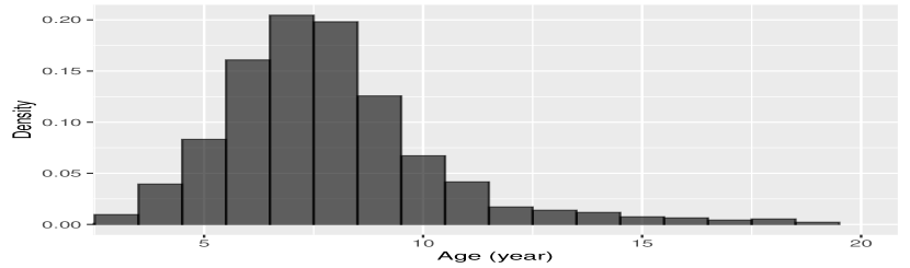
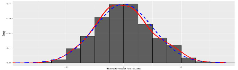
Figure 5: Left: histogram of abalone age. Right: “back-transformed” SPEUS residuals, the associated density estimate (red solid curve), and the standard normal density (blue dashed curve).

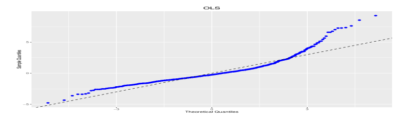
(a) OLS

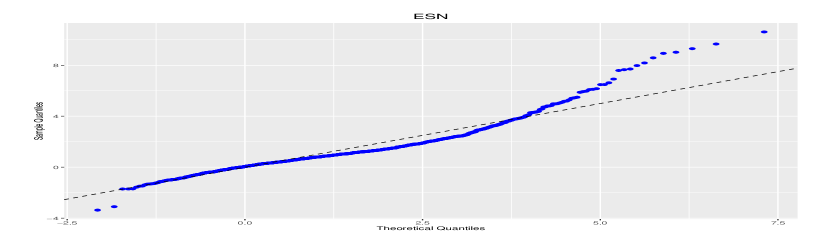
(b) ESN

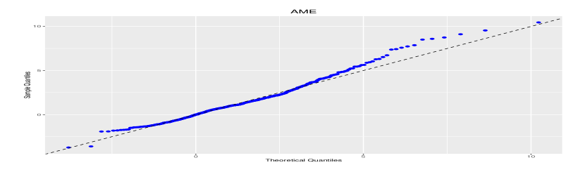
(c) AME

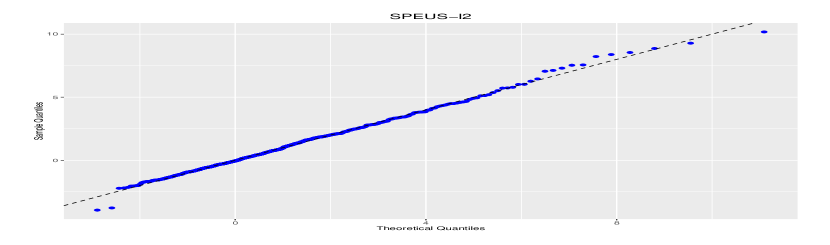
(d) SPEUS

Figure 6: Q-Q plots of model residuals on the abalone data.

To assess the goodness of fit of several different models, we present Q-Q plots of the residuals in Figure 6. Although OLS is widely adopted for the data, it clearly demonstrates a lack of fit. The ESN and AME models offer significant improvement through scale and tail adjustments, but their Q-Q plots still exhibit substantial right-skewness. In contrast, the sample quantiles in the SPEUS model nearly match the theoretical quantiles. The symmetry after the back-transform, as shown in the right panel of Figure 5, corroborates this point.

To compare the fit of the methods, which optimize different criteria based on various distributional assumptions, we conducted Kolmogorov-Smirnov tests and calculated the associated p-values: 0.008 for OLS, 0.003 for ESN, 0.08 for AME, and 0.3 for SPEUS. These findings validate our model’s superior fit. It effectively addresses pivotal point and skew effects in the data, surpassing alternative approaches that rely solely on adjustments to intercept and scale.

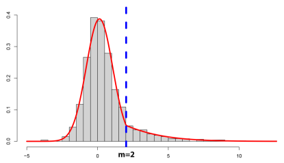
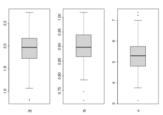
Figure 7: Abalone data. Left: Histogram of SPEUS residuals with a labeled pivotal point. Right: Bootstrap estimates of $m,\sigma,\nu$ (with 100 replications), where $m\neq 0$ and $\sigma\neq\nu$ are significant.

Figure 7 shows the histogram of the SPEUS residuals along with the bootstrap results for $m,\sigma,\nu$. The scale estimates $\hat{\sigma}=0.9$, $\hat{\nu}=5.4$, with $90\%$ confidence intervals $[0.8,1.0]$ and $[4.0,6.5]$, respectively, suggest significant skewness in the data compared to a standard Gaussian distribution. The estimated pivotal point, $\hat{m}=2$ (with a 90% confidence interval $[1.7,2.2]$) is likely associated with the legal minimum size limits in Tasmania during the 1980s (where and when the data were collected). The determination of size limits included adding an estimated two years’ growth to the size at which abalone reached sexual maturity in different areas, aiming to ensure abalone could reproduce before being harvested (Tarbath,, 1999). However, blacklip abalone do not mature in size, and the significant growth variability among various abalone stocks led to frequent changes in size limits, impacting abalone of various ages. Our estimated pivotal point appears to correspond with the 2-year protection regulation.

5.3 Medical Expenditure

Modeling medical cost data and identifying relevant predictors are valuable yet demanding tasks. MEPS conducts large-scale surveys across the United States and provides nationally representative information about medical expenditures. We model medical expenditures on 17 features on a subset (stratum ID 2109, third PSU) of the 2019 MEPS data, which includes 150 participants. Of the 17 features, 15 are from Linero et al., (2020), including, for example, the amount of total utilization of prescribed medications (RXTOT19), the number of dental care visits in 2019 (DVTOT19), age (AGE19X), each participant’s rating about their own health status (RTHLTH31), and categorized family income (POVCAT19). We also include the variables SEX and ACTLIM31, with the latter being a binary variable indicating whether a participant has any physical restrictions that impede his/her ability to engage in physical labor.

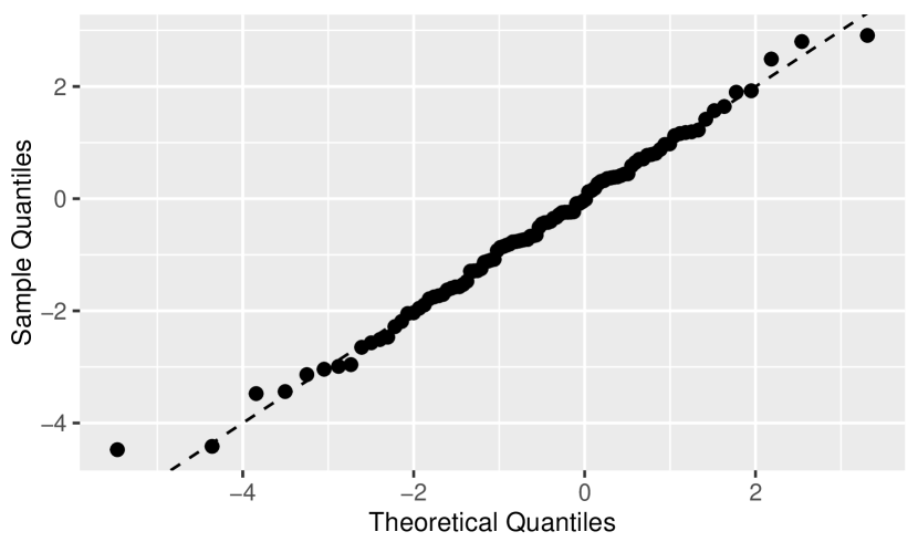
Figure 8: Q-Q plots of the continuous-part residuals on MEPS. The left panel corresponds to the standard log-normal two-part model and the right panel corresponds to its skewness-enhanced counterpart.

Traditional medical cost data analysis often employs a two-part model with logistic and log-normal components. We compared this to the sparse skewed two-part model (cf. Section 3) using a logarithmic function for $T$ and Huber’s loss for $\rho$. The regularization parameter is tuned by 5-fold selective cross-validation (She and Tran,, 2019). Figure 8 demonstrates the superior fit of the latter in terms of the continuous component. In binary component analysis, 100 repeated classification tests on 75/25 training/test splits show that our method improved accuracy from 78% to 84%.

Figure 9: Selection frequencies of the top 10 MEPS features over the 100 bootstrap replications.

Next, we analyze the variable selection outcomes using the proposed model. By bootstrapping the data 100 times, we plot the selection frequencies of the top 10 variables in Figure 9. It is worth noting that setting $\sigma=\nu$ resulted in all variables being selected at low frequencies, less than $23\%$. This emphasizes the profound influence of skewness on variable selection.

According to Figure 9, the first 4 variables, RXTOT19, DVTOT19, AGE19X, and RTHLTH31, exhibit high selection frequencies ($>60\%$). In contrast, other variables exhibited significantly lower selection frequencies. Below, we provide some practical explanation and guidance regarding these four variables.

First, RXTOT19, representing the count of a person’s total prescribed medications, is identified as highly influential in predicting medical expenditures. This predictor has the highest correlation (0.43) with the response among all the predictors. Our conclusion is consistent with Holle et al., (2021), highlighting that prescribed medication expenses constitutes a substantial portion of medical costs in the USA. Moreover, the patient’s age (AGE19X) and self-perceived health status (RTHLTH31) emerge as significant predictors influencing medical costs. This discovery aligns with Axon and Kamel, (2021).

Perhaps interestingly, our analysis also reveals that the number of dental care visits (DVTOT19), selected over 90% of the time, plays a significant role in determining the total medical costs. Its contribution appears to be unique, as it has low correlations ($<0.09$) with the other three major predictors (the number of prescriptions, self-perception, and age). Beyond the direct costs of dental care, a plausible explanation could be that individuals with regular dental visits may be more health-conscious and have higher incomes, making them more willing to spend on healthcare.

6 Summary

Skewness poses a significant challenge in data science, and many approaches attempt to model skewness by introducing different scales based on the median of a symmetric, unimodal density. This paper introduced a novel two-piece density family constructed through skewed pivot-blend. “Pivot” refers to the central reference point around which different affine transformations are applied to two conditional densities, and it can be positioned anywhere. “Blend” signifies the merging of these asymmetrically scaled densities using appropriate mixings to create a new continuous density.

We proposed a joint modeling framework that simultaneously estimates scales, the pivotal point, and other location parameters. In particular, we argued that the pivotal point does not correspond to the intercept when skewness is present, a key aspect previously overlooked in the literature. In practice, the inclusion of a single pivotal point parameter significantly enhances a model’s capacity in real-world applications.

As an important application, the paper also investigated sparse skewed two-part models, a problem that has recently gained much attention in biomedical and econometric studies. Our non-asymptotic analysis showcases how skewness in random samples, especially those with potentially heavy tails, can affect statistical accuracy. The quantification of the impact of asymmetrical scales on the choice of regularization parameters and the rates of statistical error provides an insightful examination of skewness within a finite-sample context.

We aim to raise data analysts’ awareness of data skew, as well as potential distortions that can arise when applying common transformations and conventional log-likelihoods. The technique of skewed pivot-blend offers an effective strategy for mitigating these challenges.

Appendix A Technical Details

Throughout the proofs, we use $C,c$ to denote positive constants, and they are not necessarily the same at each occurrence. Given a matrix $A$, we use $\mathcal{R}(A)$ to denote the column space (range) of $A$ and $A^{+}$ to denote the Moore-Penrose inverse of $A$. Denote by $P_{A}=A(A^{T}A)^{+}A^{T}$ the orthogonal projection on $\mathcal{R}(A)$.

A.1 Basics

The conventional definition of Orlicz $\psi$-norms goes as follows: Given a strictly increasing convex function $\psi$ on $\mathbb{R}_{+}:=[0,+\infty)$ with $\psi(0)=0$, then the Orlicz $\psi$-norm of a random variable $Y$ is defined as $\|Y\|_{\psi}=\inf\{t>0:\mathbb{E}\psi(|Y|/t)\leq 1\}$.

Some well-known examples of Orlicz $\psi$-norms are the $L_{q}$-norms: $\|Y\|_{q}=(\mathbb{E}|Y|^{q})^{1/q}$ associated with $\psi(x)=x^{q}$ $(q\geq 1)$ (e.g., the Pareto distribution), and the $\psi_{q}$-norms ($q\geq 1$) with

$$\psi_{q}(x)=\exp(x^{q})-1.$$ (A.1)

(A.1) encompasses both sub-Gaussian and sub-Exponential type random variables for $q=2,1$, without the requirement for the random variables to be centered.

Our upcoming theorems often relax the strict requirements of strict monotonicity and convexity for $\psi$. This flexibility allows us to handle random variables with much heavier tails. For instance, we consider the extension of (A.1), known as sub-Weibull random variables, which have finite $\psi_{q}$-norms for $q>0$ (cf. Kuchibhotla and Chakrabortty, (2022)). As $0<q<1$, $\psi_{q}$ is nonconvex, and these random variables, including Weibull, exhibit heavier tails compared to sub-Exponential ones (Götze et al.,, 2021).

Throughout the paper, when we refer to the Orlicz norm of a random variable, denoted as $\|\cdot\|_{\psi}$ or sometimes $\|\cdot\|_{\varphi}$, it is always understood that $\psi(\cdot)$ (or $\varphi(\cdot)$) is an nondecreasing function defined on $\mathbb{R}_{+}$ with $\psi(0)=0$. Theorem 1 also requires $\psi$ to satisfy the regularity condition $\allowbreak\limsup_{x,y\to\infty}\psi(x)\psi(y)/\psi(cxy)\allowbreak<\infty$ for some constant $c>0$ (van der Vaart and Wellner,, 2013). It is easy to verify that all these conditions are met by $L_{q}$ with $q>0$ and $\psi_{q}$ with $0<q\leq 2$. Orlicz norms provide a useful framework for analyzing skewed random variables, including those without zero mean.

In this paper, we define that a random vector $\epsilon\in\mathbb{R}^{n}$ has its Orlicz $\psi$-norm $\|\epsilon\|_{\psi}$ bounded above by $\omega$ if

$$\|\langle\epsilon,\alpha\rangle\|_{\psi}\leq\omega\|\alpha\|_{2},\ \forall\alpha\in\mathbb{R}^{n}.$$ (A.2)

Note that (A.2) is defined using the Euclidean norm $\|\cdot\|_{2}$, and the function $\psi$ may not necessarily be convex. Furthermore, the components of $\epsilon$ are not required to be independent or centered. However, if $\epsilon$ does have centered, independent components, its vector Orlicz $\psi$-norm is bounded by the largest Orlicz $\psi$-norm among its components (up to a multiplicative constant)..

Lemma A.1.

Let $\epsilon_{1},\ldots,\epsilon_{n}$ be centered, independent random variables satisfying $\|\epsilon_{i}\|_{\psi_{q}}\leq\omega$ for some $q\in(0,2]$. Given any $\alpha\in\mathbb{R}^{n}$, we have $\|\langle\alpha,\epsilon\rangle\|_{\psi_{q}}\leq C\|\alpha\|_{2}\omega$, where $C$ is a constant depending on $q$ only.

To prove the lemma, we first introduce two lemmas. The first is Theorem 1.5 in Götze et al., (2021).

Lemma A.2.

Let $\epsilon_{1},\ldots,\epsilon_{n}$ be independent random variables satisfying $\|\epsilon_{i}\|_{\psi_{q}}\leq\omega$ for some $q\in(0,2]$. Let $f(\epsilon):\mathbb{R}^{n}\to\mathbb{R}$ be a polynomial of degree $D\in\mathbb{N}$ and denote by $f^{(d)}$ the $d$-tensor of its $d$-th order partial derivatives for $1\leq d\leq D$. Then for all $t>0$, we have

$$\mathbb{P}(|f(\epsilon)-\mathbb{E}f(\epsilon)|\geq t)\leq 2\exp\big{(}-C\min_{1\leq d\leq D}(\frac{t}{\omega^{d}\|\mathbb{E}f^{(d)}(\epsilon)\|_{HS}})^{\frac{q}{d}}\big{)},$$ (A.3)

where $C$ is a constant that depends on $D$ and $q$ and $\|\cdot\|_{HS}$ denotes the Hilbert-Schmidt norm (or the Frobenius norm in the case of a matrix).

The second fact is a slight modification of Lemma 2.2.1 in van der Vaart and Wellner, (2013).

Lemma A.3.

Let $X$ be a random variable such that for some $q>0$,

$$P(|X|>t)\leq c\exp\big{(}-\big{(}\frac{t}{\omega}\big{)}^{q}\big{)},\quad\forall t>0,$$ (A.4)

where $\omega>0$ and $c$ is constant, then we have $\|X\|_{\psi_{q}}\lesssim\omega$.

The proof is straightforward:

$$\mathbb{E}\big{(}\exp(M|X|^{q})-1\big{)}=\, \mathbb{E}\int^{|X|^{q}}_{0}M\exp(Mu)\,\mathrm{d}u$$

$$=\, \int^{\infty}_{0}\mathbb{P}(|X|>u^{\frac{1}{q}})M\exp(Mu)\,\mathrm{d}u$$

$$=\, \int^{\infty}_{0}cM\exp(Mu-\frac{u}{\omega^{q}})\,\mathrm{d}u\leq\frac{cM}{\omega^{-q}-M}.$$

It suffices to take $M^{-1/q}\geq c^{\prime}\omega$ to have $\mathbb{E}(\exp(M|X|^{q})-1)\leq 1$. Therefore, $\|X\|_{\psi_{q}}\lesssim\omega$.

Now, given any $\alpha\in\mathbb{R}^{n}$, let $f_{\alpha}(\epsilon)=\langle\alpha,\epsilon\rangle=\sum^{n}_{i=1}\alpha_{i}\epsilon_{i}$. Then (i) $f_{\alpha}(\epsilon)$ is an 1-degree polynomial of $\epsilon_{1},\ldots,\epsilon_{n}$, (ii) $\|\mathbb{E}[\nabla f_{\alpha}(\epsilon)]\|_{2}=\|\alpha\|_{2}$ and $\mathbb{E}[\sum^{n}_{i=1}\alpha_{i}\epsilon_{i}]=0$, and (iii) $\epsilon_{1},\ldots,\epsilon_{n}$ are independent and satisfy $\|\epsilon_{i}\|_{\psi_{q}}\leq\omega$. Applying Lemma A.2 with $D=1,d=1$ yields

$$\mathbb{P}\big{(}|\sum^{n}_{i=1}\alpha_{i}\epsilon_{i}|>t\big{)}=\mathbb{P}\big{(}|f_{\alpha}(\epsilon)|>t\big{)}\leq 2\exp\Big{(}-C\big{(}\frac{t}{\omega\|\alpha\|_{2}}\big{)}^{q}\Big{)},$$ (A.5)

where $C$ is a constant depending on $q$ only. By Lemma A.3, (A.5) implies $\|\langle\alpha,\epsilon\rangle\|_{\psi_{q}}\leq C\|\alpha\|_{2}\omega$, where $C$ is a constant depending on $q$ only. The proof of Lemma A.1 is complete.

The following lemma is useful for stating the assumptions on effective noises.

Lemma A.4.

Let $\psi,\varphi$ be any two nondecreasing nonzero functions defined on $\mathbb{R}_{+}$ with $\psi(0)=\varphi(0)=0$ (not necessarily convex). Define $\varphi^{-1}(t):=\sup\{x\in\mathbb{R}_{+}:\varphi(x)\leq t\}.$ and $\psi^{-1}$ similarly. (i) Suppose that $\psi(\varphi^{-1}(t)/c_{0})$ is concave in $t$ on $\mathbb{R}_{+}$ for some $c_{0}>\varphi^{-1}(1)/\psi^{-1}(1)$. Then for any random variable $X$, we have $\|X\|_{\psi}\leq c_{0}\|X\|_{\varphi}$. (ii) Suppose that $\psi(\varphi^{-1}(t)/c_{0})\leq t$ for some $c_{0}>0$, then $\|X\|_{\psi}\leq c_{0}\|X\|_{\varphi}$.

We remark that the condition for $c_{0}$ in part (i) can be replaced by $c_{0}\geq\varphi^{-1}(1)/\psi^{-1}(1)$ when $\psi$ is continuous at $1$. For completeness, we provide the proof below.

First, by the definition of $\varphi^{-1}$, $u\leq\varphi^{-1}(\varphi(u))$ for any $u\geq 0$. Therefore, $X/\|X\|_{\varphi}\leq\varphi^{-1}\big{\{}\varphi(X/\|X\|_{\varphi})\big{\}}$, from which it follows that

$$\psi\Big{(}\frac{X}{c\|X\|_{\varphi}}\Big{)}\leq\psi\Big{[}\frac{1}{c}\varphi^{-1}\big{\{}\varphi(\frac{X}{\|X\|_{\varphi}})\big{\}}\Big{]}.$$ (A.6)

To prove part (i), let $f(u)=\psi\big{(}\varphi^{-1}(u)/c\big{)}$ with $c>0$ to be determined. Then $f(u)$ is an increasing function on $\mathbb{R}_{+}$. (In fact, for any $u\geq u^{\prime}\geq 0$, $\varphi^{-1}(u^{\prime})\leq\varphi^{-1}(u)$, and so $\psi\{\varphi^{-1}(u^{\prime})/c\}\leq\psi\{\varphi^{-1}(u)/c\}$.) From (A.6), picking $t=\varphi(X/\|X\|_{\varphi})$ gives

$$\psi\Big{(}\frac{X}{c\|X\|_{\varphi}}\Big{)}\leq\psi\Big{[}\frac{1}{c}\varphi^{-1}\big{\{}\varphi(\frac{X}{\|X\|_{\varphi}})\big{\}}\Big{]}=f(t).$$ (A.7)

With $c>\varphi^{-1}(1)/\psi^{-1}(1)$ (or $c\geq\varphi^{-1}(1)/\psi^{-1}(1)$ when $\psi$ is continuous at $1$), we can use Jensen’s inequality to get

$$\mathbb{E}\Big{\{}\psi\Big{(}\frac{X}{c\|X\|_{\varphi}}\Big{)}\Big{\}}\leq\mathbb{E}\Big{(}\psi\Big{[}\frac{1}{c}\varphi^{-1}\big{\{}\varphi(\frac{X}{\|X\|_{\varphi}})\big{\}}\Big{]}\Big{)}=\mathbb{E}\big{(}f(t)\big{)}\leq f\big{(}\mathbb{E}(t)\big{)}\leq f(1)\leq 1.$$ (A.8)

To prove part (ii), we still set $f(u)=\psi\big{(}\varphi^{-1}(u)/c\big{)}$ with $c>0$ and $t=\varphi(X/\|X\|_{\varphi})$. Based on (A.6), we get

$$\psi\big{(}\frac{X}{c\|X\|_{\varphi}}\big{)}\leq f(t)\leq t=\varphi\big{(}\frac{X}{\|X\|_{\varphi}}\big{)}.$$ (A.9)

The proof of Lemma A.4 is complete.

A.2 An Excess Risk Bound

This part establishes an excess risk bound for location estimation using pivot-blend, which is uniform in scale parameters, shedding light on the impact of asymmetrical scales (skewness) and the presence of an unknown pivotal point. This result is non-asymptotic and non-parametric, making it applicable to various scenarios.

Let $y_{i}\in\mathbb{R}$ and $X_{i}\in\mathbb{R}^{p}$ which satisfy satisfy $(X_{i},y_{i})\overset{i.i.d.}{\sim}F^{*}$, where $F^{*}$ is a distribution that depends on $\beta^{*},m^{*},\sigma^{*},\nu^{*}$, where we use superscript ^∗ to denote the statistical truth. As discussed in Section 2.3, we consider the practice of estimating the scales beforehand and then minimizing a criterion over all location parameters $\beta_{j}(1\leq j\leq p),m$. For ease of presentation, given $(\sigma,\nu)$, let $l_{\sigma,\nu}(\cdot;X_{i},y_{i})$, imposed on $\theta:=(\beta,m)$, denote a loss motivated by skewed pivot-blend:

$$\begin{split}l_{\sigma,\nu}(\theta;X_{i},y_{i}):=\,&\,\rho\big{(}\frac{r_{i}-m}{\sigma}+m\big{)}1_{r_{i}-m\leq 0}+\rho\big{(}\frac{r_{i}-m}{\nu}+m\big{)}1_{r_{i}-m>0}\\ &+\chi_{0}\log\big{[}\sigma\Phi(m)+\nu\{1-\Phi(m)\}\big{]}\quad\mbox{with}\quad r_{i}=y_{i}-X^{T}_{i}\beta,\end{split}$$ (A.10)

where the calibration parameter $\chi_{0}>0$ and $0\leq\Phi(m)\leq 1$. Note that $\Phi$ is not necessarily directly associated with $\rho$. Define $\hat{\theta}_{\sigma,\nu}$ by empirical risk minimization

$$\hat{\theta}_{\sigma,\nu}=\operatorname*{arg\,min}_{\theta}\sum^{n}_{i=1}l_{\sigma,\nu}(\theta;X_{i},y_{i}).$$ (A.11)

Certainly, opting for different values of $\sigma$ and $\nu$ produces diverse asymmetric losses and influences the overall risk. In our analysis, no restrictions will be placed on $\sigma$ and $\nu$. The values of $(\sigma,\nu)$ can be specified based on domain knowledge or determined in a data-dependent manner. For notational simplicity, we sometimes abbreviate $\hat{\theta}_{\sigma,\nu}$ as $\hat{\theta}$ when there is no ambiguity.

To evaluate the generalization performance of $\hat{\theta}$, let $(X_{0},y_{0})$ be a new observation that follows $F^{*}$ but is independent of the training data $(X_{i},y_{i}),(1\leq i\leq n)$, and define the population risk of $\hat{\theta}$ by

$$R_{\sigma,\nu}(\hat{\theta}):=\mathbb{E}_{(X_{0},y_{0})}\big{[}l_{\sigma,\nu}(\hat{\theta};X_{0},y_{0})\big{]},$$ (A.12)

where the expectation is taken with respect to the new observation $(X_{0},y_{0})$ only. Due to the finite number of observations in estimation, $R_{\sigma,\nu}(\hat{\theta}_{\sigma,\nu})$ is always greater than the population risk of the ideal $\theta^{*}_{\sigma,\nu}=\operatorname*{arg\,min}_{\theta}R_{\sigma,\nu}(\theta)$, or $R_{\sigma,\nu}(\theta^{*}_{\sigma,\nu})=\inf_{\theta\in\Omega}R_{\sigma,\nu}(\theta)$. In such a setup, the notion of excess risk $\mathcal{E}(\hat{\theta}_{\sigma,\nu};\sigma,\nu)$ is helpful (Devroye et al.,, 1996):

$$\mbox{Excess Risk:}\quad\mathcal{E}(\hat{\theta}_{\sigma,\nu};\sigma,\nu)\,:=\,R_{\sigma,\nu}(\hat{\theta}_{\sigma,\nu})-R_{\sigma,\nu}(\theta^{*}_{\sigma,\nu}).$$ (A.13)

Our main objective is to establish a non-asymptotic bound for $\mathcal{E}(\hat{\theta}_{\sigma,\nu};\sigma,\nu)$ regardless of the data distribution for a broad range of $\rho$ that satisfy the following assumption.

$\mathrm{ASSUMPTION}$ $\mathcal{A}$: Assume that the loss $\rho$ satisfies (i) $\rho$ is bounded: $\rho\in[0,B]$ for some $B>0$, and (ii) $\rho$ is regular in the sense that $\rho$ is piecewise polynomial on $K\geq 1$ intervals $\rho(t)=P_{i}(t),\,\forall t\in[u_{i-1},u_{i}),\,i=1,\ldots,K,$ where $u_{0}=-\infty,u_{K}=\infty$, and each polynomial function $P_{i}$ has degree at most $D\geq 0$.

Assumption $\mathcal{A}$ encompasses a wide range of practically used loss functions in robust regression and classification, specifically designed to handle extreme outliers. For example, some loss functions like $\rho(t)=\int_{0}^{|t|}\psi(s)\,\mathrm{d}s$, with a redescending $\psi$, such as Tukey’s bisquare $\psi(t)=t\{1-(t/c)^{2}\}^{2}$ if $|t|\leq c$, and $0$ otherwise (Hampel et al.,, 2011), fit in the category. Some other $\rho$ functions can be effectively approximated by piecewise polynomial functions.

Theorem A.1.

As long as the loss $\rho$ satisfies Assumption $\mathcal{A}$, the estimator $\hat{\theta}_{\sigma,\nu}$ defined in (A.11) satisfies the following probabilistic bound for all $\sigma,\nu>0$,

$$\mathbb{P} \left\{\sup_{\sigma,\nu>0}\,\mathcal{E}(\hat{\theta}_{\sigma,\nu};\sigma,\nu)-C\Bigg{[}\right.\frac{B\sqrt{p\log\big{\{}(K+1)(D+1)\big{\}}}}{\sqrt{n}}+\frac{(B\lor\chi_{0})\big{\{}\log\frac{\sigma\lor\nu}{\sigma\land\nu}+|\log(\sigma\land\nu)|\big{\}}}{\sqrt{n}}\times$$

$$\quad\quad\,\,\,\,\,\bigg{\{}\sqrt{\log\Big{(}\log\frac{\sigma\lor\nu}{\sigma\land\nu}\lor|\log(\sigma\land\nu)|\lor 1\Big{)}}+\sqrt{\log\frac{1}{\epsilon}}\bigg{\}}\left.\Bigg{]}\leq 0\right\}\geq 1-\epsilon.$$

The theorem provides a bound for the excess risk $\mathcal{E}(\hat{\theta}_{\sigma,\nu};\sigma,\nu)$ that holds uniformly in $\sigma$ and $\nu$ with probability at least $1-\epsilon$, as characterized by the following rate

$$\frac{B\sqrt{p\log\big{\{}(K+1)(D+1)\big{\}}}}{\sqrt{n}}+\frac{B\lor\chi_{0}\big{\{}\log\frac{\sigma\lor\nu}{\sigma\land\nu}+|\log(\sigma\land\nu)|\big{\}}}{\sqrt{n}}\times\bigg{\{}\sqrt{\log\frac{1}{\epsilon}}+$$

$$\quad\sqrt{\log\Big{(}\log\frac{\sigma\lor\nu}{\sigma\land\nu}\lor|\log(\sigma\land\nu)|\lor 1\Big{)}}\bigg{\}}.$$ (A.14)

The first term in (A.2) illustrates the influence of loss complexity and problem dimensions on the excess risk. The second term, which incorporates both $\sigma$ and $\nu$, arises due to the pivot estimation. Clearly, when there is no skewness, $\sigma=\nu\Rightarrow\log\frac{\sigma\lor\nu}{\sigma\land\nu}=0$ and the rate becomes

$$\frac{B\sqrt{p\log\big{\{}(K+1)(D+1)\big{\}}}}{\sqrt{n}}+\frac{(B+\chi_{0})|\log(\sigma\land\nu)|}{\sqrt{n}}\times\bigg{\{}\sqrt{\log(1+|\log(\sigma\land\nu)|)}+\sqrt{\log\frac{1}{\epsilon}}\bigg{\}}.$$

In the more practical scenario of unequal scales, the risk for location estimation can significantly increase, and the provided bound quantitatively characterizes how skewness inflates the risk non-asymptotically.

To prove the theorem, we first introduce a basic excess-risk bound for fixed $\sigma,\nu>0$.

Lemma A.5.

Suppose that the loss $\rho$ satisfies Assumption $\mathcal{A}$. Fixing the values of $\sigma,\nu>0$ in (A.10), the corresponding estimator $\hat{\theta}_{\sigma,\nu}$ from (A.11) satisfies

$$\mathcal{E}(\hat{\theta}_{\sigma,\nu};\sigma,\nu)\lesssim B\sqrt{\frac{p\log\big{\{}(K+1)(D+1)\big{\}}}{n}}+\frac{B\lor\chi_{0}\big{(}|\log\sigma\wedge\nu|+\log\frac{\nu\vee\sigma}{\sigma\wedge\nu}\big{)}}{\sqrt{n}}\sqrt{\log\frac{1}{\epsilon}},$$ (A.15)

with probability at least $1-\epsilon$.

Proof.

Let $\{X,y\}$ denote the training data, i.e., $\{X,y\}:=\big{\{}(X_{i},y_{i}),1\leq i\leq n\big{\}}$ with $(X_{i},y_{i})\overset{i.i.d.}{\sim}F^{*}$. Given $\sigma,\nu>0$, define a function class consisting of all $l_{\sigma,\nu}(\theta;\cdot)$ $\theta\in\Omega=\mathbb{R}^{p}\times\mathbb{R}$

$$\mathcal{L}_{\sigma,\nu}(\Omega):=\big{\{}l_{\sigma,\nu}(\theta;\cdot):\theta\in\Omega\big{\}}.$$ (A.16)

For simplicity, we often use the shorthand notations $R(\cdot)$, $R^{(n)}(\cdot)$, and $l(\theta;\cdot)$ to denote $R_{\sigma,\nu}(\cdot)$, $(1/n)\sum^{n}_{i=1}l_{\sigma,\nu}(\cdot;X_{i},y_{i})$, and $l_{\sigma,\nu}(\theta;\cdot)$, respectively, when there is no ambiguity.

First, the standard bound for excess risk through uniform laws yields

$$R(\hat{\theta}_{\sigma,\nu})-R(\theta^{*}_{\sigma,\nu})\leq \,R(\hat{\theta}_{\sigma,\nu})-R^{(n)}(\hat{\theta}_{\sigma,\nu})+R^{(n)}(\hat{\theta}_{\sigma,\nu})-R^{(n)}(\theta^{*}_{\sigma,\nu})+R^{(n)}(\theta^{*}_{\sigma,\nu})-R(\theta^{*}_{\sigma,\nu})$$

$$\leq \,2\sup_{\theta\in\Omega}\big{|}R(\theta)-R^{(n)}(\theta)\big{|}=2\sup_{l\in\mathcal{L}_{\sigma,\nu}(\Omega)}\big{|}\mathbb{P}_{n}l-\mathbb{P}l\big{|}=2\big{\|}\mathbb{P}_{n}-\mathbb{P}\big{\|}_{\mathcal{L}_{\sigma,\nu}(\Omega)},$$ (A.17)

where $\mathbb{P}$ is the distribution $F^{*}$ and $\mathbb{P}_{n}$ is the empirical measure that places probability mass $1/n$ on each $(X_{i},y_{i}),1\leq i\leq n$.

Let

$$g_{\sigma,\nu}(m):=\chi_{0}\log\big{[}\sigma\Phi(m)+\nu\{1-\Phi(m)\}\big{]}.$$ (A.18)

Without loss of generality, we assume that $\sigma\leq\nu$, that is, $\sigma\land\nu=\sigma,\,\sigma\lor\nu=\nu$, then

$$g_{\sigma,\nu}(m)=\chi_{0}\log\sigma+\chi_{0}\log\big{[}1+(\frac{\nu}{\sigma}-1)\{1-\Phi(m)\}\big{]}.$$ (A.19)

Because $\log(1+(\frac{\nu}{\sigma}-1)t)$ is an increasing function for $t\geq 0$, we know

$$\chi_{0}\log\sigma\leq g_{\sigma,\nu}(m)\leq\chi_{0}\log\sigma+\chi_{0}\log\frac{\nu}{\sigma},$$ (A.20)

from which it follows that

$$|g_{\sigma,\nu}(m)|\leq\big{|}\chi_{0}\log\sigma+\chi_{0}\log\frac{\nu}{\sigma}\big{|}\lor|\chi_{0}\log\sigma|\leq|\chi_{0}\log\sigma|+\chi_{0}\log\frac{\nu}{\sigma}.$$ (A.21)

By Assumption $\mathcal{A}$ and (A.21),

$$|l_{\sigma,\nu}|\leq|\rho|+|g_{\sigma,\nu}|\leq B+\chi_{0}\big{(}|\log\sigma|+\log\frac{\nu}{\sigma}\big{)}.$$ (A.22)

Due to (A.22) and $(X_{i},y_{i})\overset{i.i.d.}{\sim}F^{*}$, applying McDiarmid’s inequality and symmetrization in empirical process theory yields a data-dependent bound with probability at least $1-\epsilon$,

$$\big{\|}\mathbb{P}_{n}-\mathbb{P}\big{\|}_{\mathcal{L}_{\sigma,\nu}(\Omega)}\leq 2\mathcal{R}_{X,y}(\mathcal{L}_{\sigma,\nu}(\Omega))+6\Big{\{}B+\chi_{0}\big{(}|\log\sigma|+\log\frac{\nu}{\sigma}\big{)}\Big{\}}\sqrt{\frac{\log(3/\epsilon)}{2n}},$$ (A.23)

where $\mathcal{R}_{X,y}(\mathcal{L}_{\sigma,\nu}(\Omega))$ is the empirical Rademacher complexity of $\mathcal{L}_{\sigma,\nu}(\Omega)$ with respect to the training data $\{X,y\}$:

$$\mathcal{R}_{X,y}(\mathcal{L}_{\sigma,\nu}(\Omega)):=\frac{1}{n}\mathbb{E}_{\epsilon}\sup_{l\in\mathcal{L}_{\sigma,\nu}(\Omega)}\sum^{n}_{i=1}\epsilon_{i}l(\theta;X_{i},y_{i}),$$ (A.24)

and $\epsilon_{i}$’s are i.i.d. Rademacher random variables; see, e.g., Theorem 3.4.5 in Giné and Nickl, (2015). Note that the expectation in (A.24) is taken with respect to $\epsilon$ only, and (A.24) depends on $\sigma,\nu$ through the function class $\mathcal{L}_{\sigma,\nu}(\Omega)$.

It remains to bound the empirical Rademacher complexity. Toward this, denote by $A_{\sigma},A_{\nu}$ two augmented design matrices

$$A_{\sigma}=-\frac{1}{\sigma}[X,(1-\sigma)1_{n}],\quad A_{\nu}=-\frac{1}{\nu}[X,(1-\nu)1_{n}],$$ (A.25)

where $1_{n}$ is a column vector of $n$ ones. Let

$$\alpha_{\sigma}=\frac{1}{\sigma}y,\quad\alpha_{\nu}=\frac{1}{\nu}y.$$ (A.26)

Suppose that $\mathrm{rank}(A_{\sigma})\leq r$ and $\mathrm{rank}(A_{\nu})\leq r$. By the singular value decomposition,

$$A_{\sigma}=U_{\sigma}D_{\sigma}V^{T}_{\sigma},\quad A_{\nu}=U_{\nu}D_{\nu}V^{T}_{\nu},$$ (A.27)

where $U_{\sigma},U_{\nu}$ are orthogonal matrices with $r$ columns: $U^{T}_{\sigma}U_{\sigma}=I_{r\times r},U^{T}_{\nu}U_{\nu}=I_{r\times r}$. Define

$$\bar{U}_{\sigma}=[U_{\sigma},\alpha_{\sigma}],\quad\bar{U}_{\nu}=[U_{\nu},\alpha_{\nu}].$$ (A.28)

Now, by the sub-additivity of sup and (A.28),

$$\,\mathcal{R}_{X,y}(\mathcal{L}_{\sigma,\nu}(\Omega))$$

$$\leq \,\frac{1}{n}\mathbb{E}_{\epsilon}\sup_{\theta\in\Omega}\langle\epsilon,\rho(A_{\sigma}\theta+\alpha_{\sigma})\rangle+\frac{1}{n}\mathbb{E}_{\epsilon}\sup_{\theta\in\Omega}\langle\epsilon,\rho(A_{\nu}\theta+\alpha_{\nu})\rangle+\frac{1}{n}\mathbb{E}_{\epsilon}\sup_{m\in\mathbb{R}}\langle\epsilon,g_{\sigma,\nu}(1m)\rangle$$

$$\leq \,\frac{1}{n}\mathbb{E}_{\epsilon}\sup_{\xi\in\mathbb{R}^{r+1}}\langle\epsilon,\rho(\bar{U}_{\sigma}\xi)\rangle+\frac{1}{n}\mathbb{E}_{\epsilon}\sup_{\xi\in\mathbb{R}^{r+1}}\langle\epsilon,\rho(\bar{U}_{\nu}\xi)\rangle+\frac{1}{n}\mathbb{E}_{\epsilon}\sup_{m\in\mathbb{R}}\langle\epsilon,g_{\sigma,\nu}(1m)\rangle.$$ (A.29)

To bound the first term in (A.2), let

$$Z(X,y,\sigma)=\bar{U}_{\sigma}=[Z_{1},\cdots,Z_{n}]^{T},$$ (A.30)

and given $\rho$, define a class of functions

$$\mathcal{F}:=\big{\{}\rho(\langle\xi,\cdot\rangle):\xi\in\mathbb{R}^{r+1}\big{\}},$$ (A.31)

which does not depend on the two scale parameters. Given $Z(X,y,\sigma)$, let $\mathbb{Q}_{n}$ be the empirical measure determined by $Z_{i}$, $1\leq i\leq n$, and

$$\|f-\tilde{f}\|^{2}_{\mathbb{Q}_{n}}:=\frac{1}{n}\sum^{n}_{i=1}\big{\{}f(Z_{i})-\tilde{f}(Z_{i})\big{\}}^{2},\quad\forall f,\tilde{f}\in\mathcal{F}.$$ (A.32)

Then

$$\frac{1}{n}\mathbb{E}_{\epsilon}\sup_{\xi\in\mathbb{R}^{r+1}}\langle\epsilon,\rho(\bar{U}_{\sigma}\xi)\rangle=\frac{1}{\sqrt{n}}\mathbb{E}_{\epsilon}\sup_{f\in\mathcal{F}}\frac{1}{\sqrt{n}}\sum^{n}_{i=1}\epsilon_{i}f(Z_{i})\leq\frac{C}{\sqrt{n}}\int^{B}_{0}\sqrt{\log\mathcal{N}(\varepsilon,\mathcal{F},\|\cdot\|_{\mathbb{Q}_{n}})}\,\mathrm{d}\varepsilon,$$ (A.33)

where the last inequality is due to Dudley’s integral bound. Because $|f|\leq B,\,\forall f\in\mathcal{F}$, by Theorem 2.6.7 in van der Vaart and Wellner, (2013) we know

$$\mathcal{N}(\varepsilon,\mathcal{F},\|\cdot\|_{\mathbb{Q}_{n}})\leq C\mathcal{V}(\mathcal{F})\big{(}\frac{cB}{\varepsilon}\big{)}^{2\mathcal{V}(\mathcal{F})},$$ (A.34)

where $\mathcal{V}(\mathcal{F})$ denotes the VC-dimension of $\mathcal{F}$ defined through the notion of subgraph (cf. Definition 3.6.8 in Giné and Nickl, (2015)). In more details, $\mathcal{V}(\mathcal{F})$ is the VC-dimension of the following $\{0,1\}$-valued function class defined on $\mathbb{R}^{r+1}\times\mathbb{R}$:

$$\mathcal{H}:=\big{\{}h_{\xi}(z,t)=1_{\rho(\langle\xi,z\rangle)>t}=\operatorname*{sign}(\rho(\langle\xi,z\rangle)-t):\xi\in\mathbb{R}^{r+1}\big{\}}.$$ (A.35)

Here, the sign function is defined by $\operatorname*{sign}(a)=1$ if $a>0$, and $0$ otherwise, and recall that $1_{\rho(\langle\xi,z\rangle)>t}$ is the indicator function of the set $\big{\{}(z,t):\rho(\langle\xi,z\rangle)>t,z\in\mathbb{R}^{r+1},t\in\mathbb{R}\big{\}}$ or the subgraph of $\rho(\langle\xi,\cdot\rangle)$ for each given $\xi$.

To bound $\mathcal{V}(\mathcal{H})$, we introduce a more general function class $\tilde{\mathcal{H}}$

$$\tilde{\mathcal{H}}:=\big{\{}\tilde{h}_{\xi,\omega_{1},\omega_{2}}(z,t)=\operatorname*{sign}\big{(}\omega_{1}\rho(\langle\xi,z\rangle)+\omega_{2}t\big{)}:\xi\in\mathbb{R}^{r+1},\omega_{1},\omega_{2}\in\mathbb{R}\big{\}},$$ (A.36)

where $\tilde{h}_{\xi,\omega_{1},\omega_{2}}(z,t)$ is defined on $(z,t)\in\mathbb{R}^{r+1}\times\mathbb{R}$ and has two additional parameters $\omega_{1}$ and $\omega_{2}$ than $h_{\xi}(z,t)$ in the definition of $\mathcal{H}$. Since $\mathcal{H}\subset\tilde{\mathcal{H}}$ (by fixing $\omega_{1}=1,\omega_{2}=-1$),

$$\mathcal{V}(\mathcal{F})=\mathcal{V}(\mathcal{H})\leq\mathcal{V}(\tilde{\mathcal{H}}).$$ (A.37)

$\tilde{\mathcal{H}}$ corresponds to the set of functions computed by a neural network $\mathbf{N}$ shown in Figure A.1. It has two computation units, one in the hidden layer with activation function $\rho$, and the other in the output layer applying a sign operation on the combined inputs $\omega_{1}\rho(\langle\xi,z\rangle)+\omega_{2}t$. Lemma A.6 is Theorem 10 in Bartlett et al., (2019) and can be proved based on Theorem 2.2 of Goldberg and Jerrum, (1995).

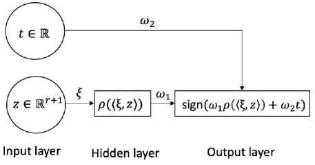
Figure A.1: Architecture of the network $\mathbf{N}$ that computes $\tilde{h}_{\xi,\omega_{1},\omega_{2}}(z,t)\in\tilde{\mathcal{H}}$.

Lemma A.6.

Suppose that a neural network $\mathbf{N}_{0}$ satisfies (i) $\mathbf{N}_{0}$ has a directed acyclic graph, that is, the connections from input or computation units to computation units do not form any loops, (ii) the unique output unit is the only computation unit in the output layer (layer $J$), where $J\geq 2$ denotes the length of the longest path in the graph of $\mathbf{N}_{0}$, and the activation function of the output unit is a sign function that takes inputs from units in any layer $j<J$, including the input layer (layer $0$), and (iii) within each computation unit except the output unit, $\Psi$ is the activation function and is piecewise polynomial on $I\geq 1$ intervals $\Psi(t)=P_{i}(t),\,\forall t\in[u_{i-1},u_{i}),i=1,\ldots,I$, where $u_{0}=-\infty,u_{I}=\infty$, and each polynomial function $P_{i}$ has degree at most $M\geq 0$. Let $W\geq 2$ be the number of parameters (weights and biases) and $U\geq 2$ be the number of computation units. Let $\mathcal{G}$ denote the set of $\{0,1\}$-valued functions computed by the network $\mathbf{N}_{0}$, then $\mathcal{V}(\mathcal{G})\leq 2W\log_{2}\big{[}16e\{M^{U-1}+\sum^{U-1}_{i=0}M^{i}\}(1+I)^{U}\big{]}$.

Our network $\mathbf{N}$ as shown in Figure A.1 is a feed-forward neural network and has a directed acyclic graph structure. The output unit of $\mathbf{N}$ in the output layer takes the input $\rho(\langle\xi,z\rangle)$ from the computation unit in the hidden layer and the input unit $t\in\mathbb{R}$ in the input layer. Under Assumption $\mathcal{A}$, our network $\mathbf{N}$ satisfies the assumptions in Lemma A.6 and has $r+3$ parameters (no bias parameters) and two computation units. Using Lemma A.6, we get

$$\mathcal{V}(\tilde{\mathcal{H}})\leq C(r+3)\log\big{\{}e(2D+1)(1+K)^{2}\big{\}}\lesssim r\log\big{\{}(K+1)(D+1)\big{\}}.$$ (A.38)

Now, based on (A.37) and (A.38),

$$\mathcal{V}(\mathcal{F})\leq Cr\log\big{\{}(K+1)(D+1)\big{\}},$$ (A.39)

and combining (A.33), (A.34), and (A.39) results in

$$\frac{1}{n}\mathbb{E}_{\epsilon}\sup_{\xi\in\mathbb{R}^{r+1}}\langle\epsilon,\rho(\bar{U}_{\sigma}\xi)\rangle\leq \,\frac{C}{\sqrt{n}}\int^{B}_{0}\sqrt{\mathcal{V}(\mathcal{F})\log\frac{B}{\varepsilon}}\,\mathrm{d}\varepsilon\lesssim B\sqrt{\frac{r\log\big{\{}(K+1)(D+1)\big{\}}}{n}}.$$ (A.40)

Similarly, the second term in (A.2) satisfies

$$\frac{1}{n}\mathbb{E}_{\epsilon}\sup_{\xi\in\mathbb{R}^{r+1}}\langle\epsilon,\rho(\bar{U}_{\nu}\xi)\rangle\lesssim B\sqrt{\frac{r\log\big{\{}(K+1)(D+1)\big{\}}}{n}}.$$ (A.41)

Note that (A.40) and (A.41) hold for all $\sigma,\nu>0$.

Finally, we bound the third term on the right-hand side of (A.2). Let

$$q_{\sigma,\nu}(m):=\chi_{0}\log\big{[}1+(\frac{\nu}{\sigma}-1)\{1-\Phi(m)\}\big{]},$$ (A.42)

and so $0\leq q_{\sigma,\nu}(m)\leq\chi_{0}\log\frac{\nu}{\sigma}$. Again, by the sub-additivity of sup and Dudley’s integral bound,

$$\frac{1}{n}\mathbb{E}_{\epsilon}\sup_{m\in\mathbb{R}}\langle\epsilon,g_{\sigma,\nu}(1m)\rangle\leq \,\frac{1}{n}\chi_{0}\log\sigma\mathbb{E}_{\epsilon}\sup_{m\in\mathbb{R}}\langle\epsilon,1\rangle+\frac{1}{n}\mathbb{E}_{\epsilon}\sup_{m\in\mathbb{R}}\langle\epsilon,q_{\sigma,\nu}(1m)\rangle$$

$$\leq \,\frac{C}{n}\int^{\frac{1}{2}\chi_{0}\log\frac{\nu}{\sigma}\sqrt{n}}_{0}\sqrt{\log\mathcal{N}\big{(}\varepsilon,\big{\{}[q_{\sigma,\nu}(1m)]:m\in\mathbb{R}\big{\}},\|\cdot\|_{2}\big{)}}\,\mathrm{d}\varepsilon$$

$$\leq \,\frac{C}{n}\int^{\frac{1}{2}\chi_{0}\log\frac{\nu}{\sigma}\sqrt{n}}_{0}\sqrt{\log\mathcal{N}\Big{(}\frac{\varepsilon}{\sqrt{n}},\big{[}0,\chi_{0}\log\frac{\nu}{\sigma}\big{]},|\cdot|\Big{)}}\,\mathrm{d}\varepsilon$$

$$\lesssim \,\frac{\chi_{0}\log\frac{\nu}{\sigma}}{\sqrt{n}}.$$ (A.43)

Plugging (A.40), (A.41), and (A.2) into (A.2) yields

$$\mathcal{R}_{X,y}(\mathcal{L}_{\sigma,\nu}(\Omega))\lesssim B\sqrt{\frac{r\log\big{\{}(K+1)(D+1)\big{\}}}{n}}+\frac{\chi_{0}\log\frac{\nu}{\sigma}}{\sqrt{n}}.$$ (A.44)

Summarizing (A.2), (A.23), and (A.44), we have the following bound with probability at least $1-\epsilon$ for any $0<\epsilon<1$,

$$\,\mathcal{E}(\hat{\theta}_{\sigma,\nu};\sigma,\nu)$$

$$\leq \,C\Bigg{[}B\sqrt{\frac{r\log\big{\{}(K+1)(D+1)\big{\}}}{n}}+\frac{\chi_{0}\log\frac{\nu}{\sigma}}{\sqrt{n}}+\frac{B+\chi_{0}\big{(}\log\frac{\nu}{\sigma}+|\log\sigma|\big{)}}{\sqrt{n}}\sqrt{\log\frac{1}{\epsilon}}\,\Bigg{]}$$

$$\lesssim \,B\sqrt{\frac{p\log\big{\{}(K+1)(D+1)\big{\}}}{n}}+\frac{B\lor\chi_{0}\big{(}\log\frac{\nu}{\sigma}+|\log\sigma|\big{)}}{\sqrt{n}}\sqrt{\log\frac{1}{\epsilon}},$$ (A.45)

where the last inequality is due to $r\leq p+1\lesssim p$. The proof of Lemma A.5 is complete. ∎

Lemma A.5 shows the effect of skewness for fixed values of $\sigma,\nu$. For example, when $\sigma=\sigma^{*},\nu=\nu^{*}$, the excess risk $\mathcal{E}(\hat{\theta}_{\sigma^{*},\nu^{*}};\sigma^{*},\nu^{*})$ satisfies

$$\mathcal{E}(\hat{\theta}_{\sigma^{*},\nu^{*}};\sigma^{*},\nu^{*})\lesssim\frac{B\sqrt{p\log\big{\{}(K+1)(D+1)\big{\}}}}{\sqrt{n}}+\frac{B\lor\chi_{0}\big{\{}\log\frac{\sigma^{*}\lor\nu^{*}}{\sigma^{*}\land\nu^{*}}+|\log(\sigma^{*}\land\nu^{*})|\big{\}}}{\sqrt{n}}\sqrt{\log\frac{1}{\epsilon}}$$ (A.46)

with probability at least $1-\epsilon$. Our objective is to establish a uniform law that applies to all scale parameters $\sigma,\nu>0$. Toward this, let

$$\tau=|\log(\sigma\land\nu)|+\log\frac{\sigma\lor\nu}{\sigma\land\nu},$$ (A.47)

which is nonnegative. By Lemma A.5, there exists a universal constant $C$ such that the event $A(\tau,t)$

$$A(\tau,t):=\left\{\mathcal{E}(\hat{\theta}_{\sigma,\nu};\sigma,\nu)-C\Bigg{[}B\sqrt{\frac{p\log\big{\{}(K+1)(D+1)\big{\}}}{n}}+\big{(}B+\chi_{0}\tau\big{)}t\Bigg{]}\geq 0\right\}$$ (A.48)

occurs with probability

$$\mathbb{P}\big{[}A(\tau,t)\big{]}\leq\exp(-2nt^{2}),$$ (A.49)

for any $t>0$.

Let $[0,+\infty)=\bigcup\limits_{l=0}^{\infty}[\tau_{l},\tau_{l+1}]$ with $0=\tau_{0}<\tau_{1}<\ldots<+\infty$ to be determined. Let $Q(\tau)\geq 0$ ($\forall\tau\geq 0$) be an increasing function. Then, for all $l\geq 0$ and $l\in\mathbb{Z}$, $\tau\in[\tau_{l},\tau_{l+1}]$ implies $\tau\geq\tau_{l}$, $Q(\tau)\geq Q(\tau_{l})$, and $\tau Q(\tau)\geq\tau Q(\tau_{l})\geq\tau_{l}Q(\tau_{l})$. Based on (A.49) and the union bound,

$$\mathbb{P}\left(\sup_{\sigma,\nu>0}\mathcal{E}(\hat{\theta}_{\sigma,\nu};\sigma,\nu)-C\Bigg{[}B\sqrt{\frac{p\log\big{\{}(K+1)(D+1)\big{\}}}{n}}+\big{(}B+\chi_{0}\tau\big{)}\big{\{}t+Q(\tau)\big{\}}\Bigg{]}\geq 0\right)$$

$$\leq \sum^{\infty}_{l=0}\mathbb{P}\Big{[}A\big{(}\tau_{l},t+Q(\tau_{l})\big{)}\Big{]}.$$ (A.50)

Take $Q(\tau)=\sqrt{\log(1+\tau)/n}$ and $\tau_{l}=l$ for all $l\geq 0$ and $l\in\mathbb{Z}$, then (A.2) is bounded by

$$\sum^{\infty}_{l=0}\mathbb{P}\Bigg{[}A\bigg{(}l,t+\sqrt{\frac{\log(1+l)}{n}}\bigg{)}\Bigg{]}\leq\sum^{\infty}_{l=0}\frac{1}{(l+1)^{2}}\exp(-2nt^{2})\leq C\exp(-2nt^{2}).$$ (A.51)

Plugging (A.47) into (A.51) gives the following uniform law for all $\sigma,\nu>0$ with probability $1-\epsilon$

$$\mathcal{E}(\hat{\theta}_{\sigma,\nu};\sigma,\nu)\leq \,C\Bigg{[}\frac{B\sqrt{p\log\big{\{}(K+1)(D+1)\big{\}}}}{\sqrt{n}}+\frac{B\lor\chi_{0}\big{\{}\log\frac{\sigma\lor\nu}{\sigma\land\nu}+|\log(\sigma\land\nu)|\big{\}}}{\sqrt{n}}$$

$$\quad\,\times\bigg{\{}\sqrt{\log\frac{1}{\epsilon}}+\sqrt{\log\big{(}\log\frac{\sigma\lor\nu}{\sigma\land\nu}\lor|\log(\sigma\land\nu)|\lor 1)+\log 2}\bigg{\}}\Bigg{]}$$

$$\lesssim \,\frac{B\sqrt{p\log\big{\{}(K+1)(D+1)\big{\}}}}{\sqrt{n}}+\frac{B\lor\chi_{0}\big{\{}\log\frac{\sigma\lor\nu}{\sigma\land\nu}+|\log(\sigma\land\nu)|\big{\}}}{\sqrt{n}}$$

$$\quad\,\times\bigg{\{}\sqrt{\log\frac{1}{\epsilon}}+\sqrt{\log\big{(}\log\frac{\sigma\lor\nu}{\sigma\land\nu}\lor|\log(\sigma\land\nu)|\lor 1)}\bigg{\}},\quad\forall\sigma,\nu>0,$$ (A.52)

The proof of Theorem A.1 is complete.

A.3 Proof of Theorem 1

By the optimality of $\hat{\mu}$: $l(\hat{\mu})+\frac{\tau}{2}\|\hat{\gamma}\|^{2}_{2}+\lambda\varrho\|\hat{\bar{\beta}}\|_{2,1}\leq l(\mu^{*})+\frac{\tau}{2}\|\gamma^{*}\|^{2}_{2}+\lambda\varrho\|\bar{\beta}^{*}\|_{2,1}$, we obtain a basic inequality as follows

$$\,\mathbf{\Delta}_{l}(\hat{\mu},\mu^{*})+\frac{\tau}{2}\|\hat{\gamma}-\gamma^{*}\|^{2}_{2}$$

$$\leq \,\big{\langle}\epsilon_{\bar{\eta}},\bar{X}\hat{\bar{\beta}}-\bar{X}\bar{\beta}^{*}\big{\rangle}+\langle\epsilon_{\bar{m}},\hat{\bar{m}}-\bar{m}\rangle+\langle\epsilon_{\varsigma},\hat{\varsigma}-\varsigma\rangle+\langle-\tau\gamma^{*},\hat{\gamma}-\gamma^{*}\rangle$$

$$\,+\lambda\varrho\|\bar{\beta}^{*}\|_{2,1}-\lambda\varrho\|\hat{\bar{\beta}}\|_{2,1}$$

$$\leq \,\big{\langle}\epsilon_{\bar{\eta}},\bar{X}\hat{\bar{\beta}}-\bar{X}\bar{\beta}^{*}\big{\rangle}+\langle\epsilon_{\bar{m}},\hat{\bar{m}}-\bar{m}\rangle+\langle\epsilon_{\varsigma},\hat{\varsigma}-\varsigma\rangle+\frac{b}{2}\|\hat{\gamma}-\gamma^{*}\|^{2}_{2}+\frac{\tau^{2}}{2b}\|\gamma^{*}\|_{2}^{2}$$

$$\,+\lambda\varrho\|\bar{\beta}^{*}\|_{2,1}-\lambda\varrho\|\hat{\bar{\beta}}\|_{2,1}$$ (A.53)

for any $b>0$.

First, we bound $\big{\langle}\epsilon_{\bar{\eta}},\bar{X}\hat{\bar{\beta}}-\bar{X}\bar{\beta}^{*}\big{\rangle}$. Let $\bar{X}_{k}$ denote the $k$th column of $\bar{X}$ and $\Xi_{k}:=[\bar{X}_{k},\bar{X}_{p+k}]^{T}$ and recall ${\bar{\beta}}_{k}=[\beta_{k},b_{k}]^{T}$, $k=1,\ldots,p$. By Hölder’s inequality,

$$\langle\epsilon_{\bar{\eta}},\bar{X}\hat{\bar{\beta}}-\bar{X}\bar{\beta}^{*}\rangle=\sum^{p}_{k=1}\langle\Xi_{k}\epsilon_{\bar{\eta}},\hat{\bar{\beta}}_{k}-\bar{\beta}^{*}_{k}\rangle\leq\sum^{p}_{k=1}\|\Xi_{k}\epsilon_{\bar{\eta}}\|_{2}\|\hat{\bar{\beta}}_{k}-\bar{\beta}^{*}_{k}\|_{2}\leq\sqrt{2}\big{\|}\bar{X}^{T}\epsilon_{\bar{\eta}}\big{\|}_{\infty}\|\hat{\bar{\beta}}-\bar{\beta}^{*}\|_{2,1}.$$ (A.54)

Let $\lambda=A\big{\|}\bar{X}^{T}\epsilon_{\bar{\eta}}\big{\|}_{\infty}/\varrho$ for $A>1$. Then we have

$$\,\big{\|}\bar{X}^{T}\epsilon_{\bar{\eta}}\big{\|}_{\infty}\big{\|}\hat{\bar{\beta}}-\bar{\beta}^{*}\big{\|}_{2,1}+\lambda\varrho\big{\|}\bar{\beta}^{*}\big{\|}_{2,1}-\lambda\varrho\big{\|}\hat{\bar{\beta}}\big{\|}_{2,1}$$

$$\leq \,\big{(}\lambda\varrho+\big{\|}\bar{X}^{T}\epsilon_{\bar{\eta}}\big{\|}_{\infty}\big{)}\big{\|}\bar{\beta}^{*}\big{\|}_{2,1}+\big{(}\big{\|}\bar{X}^{T}\epsilon_{\bar{\eta}}\big{\|}_{\infty}-\lambda\varrho\big{)}\big{\|}\hat{\bar{\beta}}\big{\|}_{2,1}$$

$$= \,(1+A)\big{\|}\bar{X}^{T}\epsilon_{\bar{\eta}}\big{\|}_{\infty}\big{\|}\bar{\beta}^{*}\big{\|}_{2,1}+(1-A)\big{\|}\bar{X}^{T}\epsilon_{\bar{\eta}}\big{\|}_{\infty}\big{\|}\hat{\bar{\beta}}\big{\|}_{2,1}$$

$$\leq \,(1+A)\big{\|}\bar{X}^{T}\epsilon_{\bar{\eta}}\big{\|}_{\infty}\big{\|}\bar{\beta}^{*}\big{\|}_{2,1}.$$ (A.55)

By the assumption on $\epsilon_{\bar{\eta}}$, the $\psi$-norm of $|\bar{X}^{T}_{k}\epsilon_{\bar{\eta}}|$ is bounded by

$$\big{\|}\bar{X}^{T}_{k}\epsilon_{\bar{\eta}}\big{\|}_{\psi}=\|\langle\epsilon_{\bar{\eta}},\bar{X}_{k}\rangle\|_{\psi}\leq\|\epsilon_{\bar{\eta}}\|_{\psi}\|\bar{X}_{k}\|_{2}\leq\omega_{\bar{\eta}}\varrho.$$ (A.56)

The following inequality is essentially Massart’s finite class lemma, adapted for our purpose

$$\big{\|}\max_{1\leq k\leq 2p}|\bar{X}^{T}_{k}\epsilon_{\bar{\eta}}|\big{\|}_{\psi}\leq 2(1\vee c_{1}\vee 2\psi(c_{2}))^{2}c_{0}\psi^{-1}(p)\omega_{\bar{\eta}}\varrho.$$ (A.57)

It can be obtained by modifying the proof of Lemma 2.2.2 in van der Vaart and Wellner, (2013) (details omitted). By Lemma A.4,

$$\mathbb{E}\big{[}\|\bar{X}^{T}\epsilon_{\bar{\eta}}\|_{\infty}\big{]}\leq\left\|\|\bar{X}^{T}\epsilon_{\bar{\eta}}\|_{\infty}\right\|_{L_{2}}\leq\psi^{-1}(1)\Big{\|}\big{\|}\bar{X}^{T}\epsilon_{\bar{\eta}}\big{\|}_{\infty}\Big{\|}_{\psi}\leq Cc_{\psi}\psi^{-1}(p)\omega_{\bar{\eta}}\varrho,$$ (A.58)

where $c_{\psi}=(1\vee c_{1}\vee 2\psi(c_{2}))^{2}c_{0}\psi^{-1}(1)$. Therefore,

$$\mathbb{E}\Big{\{}\big{\langle}\epsilon_{\bar{\eta}},\bar{X}\hat{\bar{\beta}}-\bar{X}\bar{\beta}^{*}\big{\rangle}+\lambda\varrho\big{\|}\bar{\beta}^{*}\big{\|}_{2,1}-\lambda\varrho\big{\|}\hat{\bar{\beta}}\big{\|}_{2,1}\Big{\}}\leq \,(1+A)\mathbb{E}\Big{[}\big{\|}\bar{X}^{T}\epsilon_{\bar{\eta}}\big{\|}_{\infty}\Big{]}\big{\|}\bar{\beta}^{*}\big{\|}_{2,1}$$

$$\leq \,C(1+A)c_{\psi}\psi^{-1}(p)\omega_{\bar{\eta}}\varrho\big{\|}\bar{\beta}^{*}\big{\|}_{2,1}.$$ (A.59)

Next, we bound the stochastic term $\langle\epsilon_{\bar{m}},\hat{\bar{m}}-\bar{m}^{*}\rangle$. For any $a>0$,

$$\langle\epsilon_{\bar{m}},\hat{\bar{m}}-\bar{m}^{*}\rangle=\langle P_{1_{n}}\epsilon_{\bar{m}},\hat{\bar{m}}-\bar{m}^{*}\rangle\leq|u^{T}\epsilon_{\bar{m}}|\cdot\|\hat{\bar{m}}-\bar{m}^{*}\|_{2}\leq a(u^{T}\epsilon_{\bar{m}})^{2}+\frac{1}{2a}\mathrm{\mathbf{D}}_{2}(\hat{\bar{m}},\bar{m}^{*}),$$ (A.60)

where $P_{1_{n}}$ is the orthogonal projection matrix onto the column space of $1_{n}$, or equivalently, $uu^{T}$ with $u=(1/\sqrt{n})1_{n}$. By Lemma A.4,

$$\mathbb{E}\big{[}(u^{T}\epsilon_{\bar{m}})^{2}\big{]}\leq\{\psi^{-1}(1)\}^{2}\|u^{T}\epsilon_{\bar{m}}\|^{2}_{\varphi}\leq\{\psi^{-1}(1)\}^{2}\omega^{2}_{\bar{m}}.$$ (A.61)

Likewise, for the stochastic term $\langle\epsilon_{\varsigma},\hat{\varsigma}-\varsigma^{*}\rangle$ with $\epsilon_{\varsigma}=[\epsilon^{T}_{\frac{1}{\sigma}1_{n}},\epsilon^{T}_{\frac{1}{\nu}1_{n}}]^{T}$ and $\hat{\varsigma}-\varsigma^{*}=[(1/\hat{\sigma}-1/\sigma^{*})1^{T}_{n},(1/\hat{\nu}-1/\nu^{*})1^{T}_{n}]^{T}$, we have

$$\,\big{\langle}\epsilon_{\frac{1}{\sigma}1_{n}},(\frac{1}{\hat{\sigma}}-\frac{1}{\sigma^{*}})1_{n}\big{\rangle}+\big{\langle}\epsilon_{\frac{1}{\nu}1_{n}},(\frac{1}{\hat{\nu}}-\frac{1}{\nu^{*}})1_{n}\big{\rangle}$$

$$= \,\big{\langle}P_{1_{n}}\epsilon_{\frac{1}{\sigma}1_{n}},(\frac{1}{\hat{\sigma}}-\frac{1}{\sigma^{*}})1_{n}\big{\rangle}+\big{\langle}P_{1_{n}}\epsilon_{\frac{1}{\nu}1_{n}},(\frac{1}{\hat{\nu}}-\frac{1}{\nu^{*}})1_{n}\big{\rangle}$$

$$\leq \,a(u^{T}\epsilon_{\frac{1}{\sigma}1_{n}})^{2}+a(u^{T}\epsilon_{\frac{1}{\nu}1_{n}})^{2}+\frac{1}{2a}\mathrm{\mathbf{D}}_{2}(\hat{\varsigma},\varsigma^{*}),$$

and

$$\mathbb{E}\big{[}(u^{T}\epsilon_{\frac{1}{\sigma}1_{n}})^{2}\big{]}\leq\{\varphi^{-1}(1)\}^{2}\|u^{T}\epsilon_{\frac{1}{\sigma}1_{n}}\|^{2}_{\varphi}\leq\{\varphi^{-1}(1)\}^{2}\omega^{2}_{\varsigma},$$

and $\mathbb{E}[(u^{T}\epsilon_{\frac{1}{\nu}1_{n}})^{2}]\leq\{\varphi^{-1}(1)\}^{2}\omega^{2}_{\varsigma}$. To sum up, for any $a>0$,

$$\,\mathbb{E}\big{\{}\langle\epsilon_{\bar{m}},\hat{\bar{m}}-\bar{m}^{*}\rangle+\langle\epsilon_{\varsigma},\hat{\varsigma}-\varsigma^{*}\rangle\big{\}}$$

$$\leq \,a\{\psi^{-1}(1)\}^{2}\omega^{2}_{\bar{m}}+2a\{\varphi^{-1}(1)\}^{2}\omega^{2}_{\varsigma}+\frac{1}{2a}\{\mathrm{\mathbf{D}}_{2}(\hat{\bar{m}},\bar{m}^{*})+\mathrm{\mathbf{D}}_{2}(\hat{\varsigma},\varsigma^{*})\}.$$ (A.62)

Plugging (A.3) and (A.3) into (A.3) to obtain

$$\,\mathbb{E}\Big{\{}\mathbb{\Delta}_{l}(\hat{\mu},\mu^{*})+(\tau-b)\mathrm{\mathbb{D}}_{2}(\hat{\gamma},\gamma^{*})\Big{\}}-\frac{1}{2a}\{\mathrm{\mathbb{D}}_{2}(\hat{\bar{m}},\bar{m}^{*})+\mathrm{\mathbb{D}}_{2}(\hat{\varsigma},\varsigma^{*})\}$$

$$\leq \,C(1+A)c_{\psi}\psi^{-1}(p)\omega_{\bar{\eta}}\varrho\big{\|}\bar{\beta}^{*}\big{\|}_{2,1}+a\{\psi^{-1}(1)\}^{2}\omega^{2}_{\bar{m}}+2a\{\varphi^{-1}(1)\}^{2}\omega^{2}_{\varsigma}+\frac{\tau^{2}}{2b}\|\gamma^{*}\|_{2}^{2}.$$ (A.63)

Choosing $b=\tau/4$, $a=2/\tau$, we get

$$\,\mathbb{E}\Big{\{}\mathbb{\Delta}_{l}(\hat{\mu},\mu^{*})+\frac{\tau}{2}\mathrm{\mathbb{D}}_{2}(\hat{\gamma},\gamma^{*})\Big{\}}$$

$$\leq \,C(1+A)c_{\psi}\psi^{-1}(p)\omega_{\bar{\eta}}\varrho\big{\|}\bar{\beta}^{*}\big{\|}_{2,1}+\frac{2}{\tau}\big{[}\{\psi^{-1}(1)\}^{2}\omega^{2}_{\bar{m}}+2\{\varphi^{-1}\}^{2}\omega^{2}_{\varsigma}\big{]}+2\tau\|\gamma^{*}\|_{2}^{2}$$

$$\lesssim \,c_{\psi}\psi^{-1}(p)\omega_{\bar{\eta}}\varrho\big{\|}\bar{\beta}^{*}\big{\|}_{2,1}+\frac{1}{\tau}(\omega^{2}_{\bar{m}}+\omega^{2}_{\varsigma})+\tau\|\gamma^{*}\|_{2}^{2}.$$ (A.64)

The proof is complete.

A.4 Proof of Theorem 2

We prove a more general result, which includes Theorem 2 as a special case.

Theorem A.2.

Assume that the effective noises $\epsilon_{\bar{\eta}},\epsilon_{\bar{m}}$, and $\epsilon_{\varsigma}$ satisfy $\|\epsilon_{\bar{\eta}}\|_{\psi}\leq\omega_{\bar{\eta}},\|\epsilon_{\bar{m}}\|_{\psi}\leq\omega_{\bar{m}}$, and $\|\epsilon_{\varsigma}\|_{\varphi}\leq\omega_{\varsigma}$. Let $\hat{\zeta}$ denote the optimal solution for (19) with $\varrho\geq\kappa_{2,\infty}$. Suppose that there exist some $\vartheta>0$ and some large $K>0$ such that the following condition holds for any $\bar{\beta},\gamma$ (recall $\zeta^{T}=[\bar{\beta}^{T},\gamma^{T}]$, $\mu^{T}=[\bar{\eta}^{T},\gamma^{T}]$ defined based on (17))

$$(1+\vartheta)\lambda\varrho\big{\|}(\bar{\beta}-\bar{\beta}^{*})_{\mathcal{J}^{*}}\big{\|}_{2,1}\leq\mathbb{\Delta}_{l}(\mu,\mu^{*})+\lambda\varrho\big{\|}(\bar{\beta}-\bar{\beta}^{*})_{\mathcal{J}^{*C}}\big{\|}_{2,1}+K\lambda^{2}J^{*},$$ (A.65)

where

$$\lambda=\big{(}1\lor\frac{1}{\vartheta}\big{)}\omega_{\bar{\eta}}\psi^{-1}\big{[}p\psi\big{\{}A\psi^{-1}(p)\big{\}}\big{]}$$ (A.66)

for some large enough $A>0$. Then for any $L,L^{\prime}>0$,

$$\begin{split}\mathbb{\Delta}_{l}(\hat{\mu},\mu^{*})+\frac{\tau}{2}\mathrm{\mathbb{D}}_{2}(\gamma,\gamma^{*})\,\lesssim\,&\,(\frac{1}{\vartheta}\lor\frac{1}{\vartheta^{3}})K\omega^{2}_{\bar{\eta}}\Big{(}\psi^{-1}\Big{[}p\psi\big{\{}A\psi^{-1}(p)\big{\}}\Big{]}\Big{)}^{2}J^{*}\\ &\,+(1\lor\frac{1}{\vartheta})\frac{1}{\tau}\big{(}L^{2}\omega^{2}_{\bar{m}}+L^{{}^{\prime}2}\omega^{2}_{\varsigma}\big{)}+(1\lor\frac{1}{\vartheta})\tau\|\gamma^{*}\|_{2}^{2}\end{split}$$ (A.67)

holds with probability at least $1-C/\psi\{A\psi^{-1}(p)\}-1/\psi(cL)-C/\varphi(cL^{\prime})$, where $C,c$ are positive constants.

Theorem A.2 implies Theorem 2. In fact, (A.65), assuming $\vartheta$ is a constant, is just (27), and letting $\psi=\psi_{q}$ for some $q>0$, (A.66) yields $\lambda=A\omega_{\bar{\eta}}(\log p)^{\frac{1}{q}}$. Then, choosing $L=C\psi^{-1}(p^{A^{q}}),L^{\prime}=C\varphi^{-1}(p^{A^{q}})$, we can obtain the result in Theorem 2:

$$\,\mathbb{\Delta}_{l}(\hat{\mu},\mu^{*})+\frac{\tau}{2}\mathrm{\mathbb{D}}_{2}(\hat{\gamma},\gamma^{*})$$

$$\lesssim \,KA^{2}\omega^{2}_{\bar{\eta}}J^{*}(\log p)^{\frac{2}{q}}+\frac{1}{\tau}\{\psi_{q}^{-1}(p^{A^{q}})\}^{2}\omega^{2}_{\bar{m}}+\frac{1}{\tau}\{\varphi^{-1}(p^{A^{q}})\}^{2}\omega^{2}_{\varsigma}+\tau\|\gamma^{*}\|_{2}^{2}$$

with probability at least $1-Cp^{-cA^{q}}$.

Proof.

From $l(\hat{\mu})+\tau\|\hat{\gamma}\|^{2}_{2}+\lambda\varrho\|\hat{\bar{\beta}}\|_{2,1}\leq l(\mu^{*})+\tau\|\gamma^{*}\|^{2}_{2}+\lambda\varrho\|\bar{\beta}^{*}\|_{2,1}$, we obtain

$$\,\mathbb{\Delta}_{l}(\hat{\mu},\mu^{*})+\frac{\tau}{2}\|\hat{\gamma}-\gamma^{*}\|^{2}_{2}$$

$$\leq \,\big{\langle}\epsilon_{\bar{\eta}},\bar{X}\hat{\bar{\beta}}-\bar{X}\bar{\beta}^{*}\big{\rangle}+\langle\epsilon_{\bar{m}},\hat{\bar{m}}-\bar{m}\rangle+\langle\epsilon_{\varsigma},\hat{\varsigma}-\varsigma\rangle+\langle-\tau\gamma^{*},\hat{\gamma}-\gamma^{*}\rangle$$

$$\,+\lambda\varrho\|\bar{\beta}^{*}\|_{2,1}-\lambda\varrho\|\hat{\bar{\beta}}\|_{2,1}$$

$$\leq \,\big{\langle}\epsilon_{\bar{\eta}},\bar{X}\hat{\bar{\beta}}-\bar{X}\bar{\beta}^{*}\big{\rangle}+\langle\epsilon_{\bar{m}},\hat{\bar{m}}-\bar{m}\rangle+\langle\epsilon_{\varsigma},\hat{\varsigma}-\varsigma\rangle+\frac{b}{2}\|\hat{\gamma}-\gamma^{*}\|^{2}_{2}+\frac{\tau^{2}}{2b}\|\gamma^{*}\|_{2}^{2}$$

$$\,+\lambda\varrho\|\bar{\beta}^{*}\|_{2,1}-\lambda\varrho\|\hat{\bar{\beta}}\|_{2,1}$$ (A.68)

for any $b>0$.

To bound $\big{\langle}\epsilon_{\bar{\eta}},\bar{X}\hat{\bar{\beta}}-\bar{X}\bar{\beta}^{*}\big{\rangle}$, we use the same notations in Appendix A.3 and recall

$$\langle\epsilon_{\bar{\eta}},\bar{X}\hat{\bar{\beta}}-\bar{X}\bar{\beta}^{*}\rangle\leq c_{0}\max_{1\leq k\leq 2p}|\bar{X}^{T}_{k}\epsilon_{\bar{\eta}}|\|\hat{\bar{\beta}}-\bar{\beta}^{*}\|_{2,1},$$ (A.69)

where the constant $c_{0}\geq\sqrt{2}$, and

$$\big{\|}\bar{X}^{T}_{k}\epsilon_{\bar{\eta}}\big{\|}_{\psi}\leq\omega_{\bar{\eta}}\varrho,\ \forall k.$$ (A.70)

Let

$$\lambda_{0}=\omega_{\bar{\eta}}\psi^{-1}\Big{[}p\psi\big{\{}A\psi^{-1}(p)\big{\}}\Big{]}$$ (A.71)

for some large enough $A>0$. By the union bound and Markov’s inequality, the event $\underset{1\leq k\leq 2p}{\max}|\bar{X}^{T}_{k}\epsilon_{\bar{\eta}}|\geq\lambda_{0}\varrho$ occurs with probability

$$\mathbb{P}(\max_{1\leq k\leq 2p}|\bar{X}^{T}_{k}\epsilon_{\bar{\eta}}|\geq\lambda_{0}\varrho)\leq \frac{2p}{\psi\Big{(}\frac{\omega_{\bar{\eta}}\varrho\psi^{-1}\big{[}p\psi\{A\psi^{-1}(p)\}\big{]}}{\omega_{\bar{\eta}}\varrho}\Big{)}}\leq\frac{2p}{{p\psi\{A\psi^{-1}(p)\}\big{]}}}\leq\frac{2}{\psi\{A\psi^{-1}(p)\}}.$$ (A.72)

Let $\lambda=\lambda_{0}/b^{\prime}$ with $b^{\prime}>0$. By the subadditivity of the $\ell_{1}$-penalty, we get

$$\,c_{0}\lambda_{0}\varrho\big{\|}\hat{\bar{\beta}}-\bar{\beta}^{*}\big{\|}_{2,1}+\lambda\varrho\big{\|}\bar{\beta}^{*}\big{\|}_{2,1}-\lambda\varrho\big{\|}\hat{\bar{\beta}}\big{\|}_{2,1}$$

$$\leq \,c_{0}\lambda_{0}\varrho\big{\|}(\hat{\bar{\beta}}-\bar{\beta}^{*})_{\mathcal{J}^{*}}\big{\|}_{2,1}+c_{0}\lambda_{0}\varrho\big{\|}(\hat{\bar{\beta}}-\bar{\beta}^{*})_{{}_{\mathcal{J}^{*C}}}\big{\|}_{2,1}+\lambda\varrho\big{\|}\bar{\beta}^{*}_{\mathcal{J}^{*}}\big{\|}_{2,1}$$

$$\,-\lambda\varrho\big{\|}\hat{\bar{\beta}}_{{}_{\mathcal{J}^{*}}}\big{\|}_{2,1}-\lambda\varrho\big{\|}(\hat{\bar{\beta}}-\bar{\beta}^{*})_{{}_{\mathcal{J}^{*C}}}\big{\|}_{2,1}$$

$$\leq \,\big{(}c_{0}\lambda_{0}+\lambda\big{)}\varrho\big{\|}(\hat{\bar{\beta}}-\bar{\beta}^{*})_{\mathcal{J}^{*}}\big{\|}_{2,1}-\big{(}\lambda-c_{0}\lambda_{0}\big{)}\varrho\big{\|}(\hat{\bar{\beta}}-\bar{\beta}^{*})_{{}_{\mathcal{J}^{*C}}}\big{\|}_{2,1}$$

$$= \,\big{(}1+c_{0}b^{\prime}\big{)}\lambda\varrho\big{\|}(\hat{\bar{\beta}}-\bar{\beta}^{*})_{\mathcal{J}^{*}}\big{\|}_{2,1}-\big{(}1-c_{0}b^{\prime}\big{)}\lambda\varrho\big{\|}(\hat{\bar{\beta}}-\bar{\beta}^{*})_{{}_{\mathcal{J}^{*C}}}\big{\|}_{2,1},$$ (A.73)

where $\mathcal{J}^{*C}$ is the complement of $\mathcal{J}^{*}$.

For the stochastic term $\langle\epsilon_{\bar{m}},\hat{\bar{m}}-\bar{m}^{*}\rangle$, for any $a>0$,

$$\langle\epsilon_{\bar{m}},\hat{\bar{m}}-\bar{m}^{*}\rangle=\langle P_{1_{n}}\epsilon_{\bar{m}},\hat{\bar{m}}-\bar{m}^{*}\rangle\leq|u^{T}\epsilon_{\bar{m}}|\cdot\|\hat{\bar{m}}-\bar{m}^{*}\|_{2}\leq a(u^{T}\epsilon_{\bar{m}})^{2}+\frac{1}{2a}\mathrm{\mathbb{D}}_{2}(\hat{\bar{m}},\bar{m}^{*}),$$ (A.74)

where $P_{1_{n}}=uu^{T}$ with $u=(1/\sqrt{n})1_{n}$. By the assumption on $\epsilon_{\bar{m}}$, $\|u^{T}\epsilon_{\bar{m}}\|_{\psi}\leq\omega_{\bar{m}}$. By Markov’s inequality,

$$\mathbb{P}\Big{(}(u^{T}\epsilon_{\bar{m}})^{2}\geq cL^{2}\omega^{2}_{\bar{m}}\Big{)}\leq\frac{1}{\psi(\frac{cL\omega_{\bar{m}}}{\omega_{\bar{m}}})}=\frac{1}{\psi(cL)},$$ (A.75)

from which it follow that

$$\langle\epsilon_{\bar{m}},\hat{\bar{m}}-\bar{m}^{*}\rangle\leq acL^{2}\omega^{2}_{\bar{m}}+\frac{1}{2a}\mathrm{\mathbb{D}}_{2}(\hat{\bar{m}},\bar{m}^{*})$$ (A.76)

occurs with probability at least $1-1/\psi(cL)$. For the stochastic term $\langle\epsilon_{\varsigma},\hat{\varsigma}-\varsigma\rangle$ with $\epsilon_{\varsigma}=[\epsilon^{T}_{\frac{1}{\sigma}1_{n}},\epsilon^{T}_{\frac{1}{\nu}1_{n}}]^{T}$ and $\hat{\varsigma}-\varsigma^{*}=[(1/\hat{\sigma}-1/\sigma^{*})1^{T}_{n},(1/\hat{\nu}-1/\nu^{*})1^{T}_{n}]^{T}$, similarly,

$$\,\big{\langle}\epsilon_{\frac{1}{\sigma}1_{n}},(\frac{1}{\hat{\sigma}}-\frac{1}{\sigma^{*}})1_{n}\big{\rangle}+\big{\langle}\epsilon_{\frac{1}{\nu}1_{n}},(\frac{1}{\hat{\nu}}-\frac{1}{\nu^{*}})1_{n}\big{\rangle}$$

$$= \,\big{\langle}P_{1_{n}}\epsilon_{\frac{1}{\sigma}1_{n}},(\frac{1}{\hat{\sigma}}-\frac{1}{\sigma^{*}})1_{n}\big{\rangle}+\big{\langle}P_{1_{n}}\epsilon_{\frac{1}{\nu}1_{n}},(\frac{1}{\hat{\nu}}-\frac{1}{\nu^{*}})1_{n}\big{\rangle}$$

$$\leq \,a(u^{T}\epsilon_{\frac{1}{\sigma}1_{n}})^{2}+a(u^{T}\epsilon_{\frac{1}{\nu}1_{n}})^{2}+\frac{1}{2a}\mathrm{\mathbb{D}}_{2}(\hat{\varsigma},\varsigma^{*}).$$

By the assumption on $\epsilon_{\varsigma}$, $\|u^{T}\epsilon_{\frac{1}{\sigma}1_{n}}\|_{\varphi}\leq\omega_{\varsigma},\|u^{T}\epsilon_{\frac{1}{\nu}1_{n}}\|_{\varphi}\leq\omega_{\varsigma}$. It follows from

$$\mathbb{P}\Big{(}(u^{T}\epsilon_{\frac{1}{\sigma}1_{n}})^{2}\geq cL^{{}^{\prime}2}\omega^{2}_{\varsigma}\Big{)}\leq\frac{1}{\psi(\frac{cL\omega_{\varsigma}}{\omega_{\varsigma}})}=\frac{1}{\psi(cL^{\prime})}$$ (A.77)

and $\mathbb{P}\Big{(}(u^{T}\epsilon_{\frac{1}{\nu}1_{n}})^{2}\geq cL^{{}^{\prime}2}\omega^{2}_{\varsigma}\Big{)}\leq 1/\psi(cL^{\prime})$ that

$$\langle\epsilon_{\varsigma},\hat{\varsigma}-\varsigma\rangle\leq 2acL^{{}^{\prime}2}\omega^{2}_{\varsigma}+\frac{1}{2a}\mathrm{\mathbb{D}}_{2}(\hat{\varsigma},\varsigma^{*}),$$ (A.78)

with probability at least $1-2/\varphi(cL^{\prime})$.

Plugging (A.72), (A.4), (A.76), and (A.78) into (A.4) results in

$$\,\mathbb{\Delta}_{l}(\hat{\mu},\mu^{*})+(\tau-b)\mathrm{\mathbb{D}}_{2}(\hat{\gamma},\gamma^{*})-\frac{1}{2a}\mathrm{\mathbb{D}}_{2}(\hat{\bar{m}},\bar{m}^{*})-\frac{1}{2a}\mathrm{\mathbb{D}}_{2}(\hat{\varsigma},\varsigma^{*})$$

$$\leq \,\big{(}1+c_{0}b^{\prime}\big{)}\lambda\varrho\big{\|}(\hat{\bar{\beta}}-\bar{\beta}^{*})_{\mathcal{J}^{*}}\big{\|}_{2,1}-\big{(}1-c_{0}b^{\prime}\big{)}\lambda\varrho\big{\|}(\hat{\bar{\beta}}-\bar{\beta}^{*})_{{}_{\mathcal{J}^{*C}}}\big{\|}_{2,1}+\frac{\tau^{2}}{2b}\|\gamma^{*}\|_{2}^{2}$$

$$\,+acL^{2}\omega^{2}_{\bar{m}}+2acL^{{}^{\prime}2}\omega^{2}_{\varsigma}.$$ (A.79)

with probability at least $1-C/\psi\{A\psi^{-1}(p)\}-1/\psi(cL)-C/\varphi(cL^{\prime})$, where $C,c$ are positive constants.

The regularity condition (A.65) implies

$$\,(1+\frac{\vartheta}{2+\vartheta})\lambda\varrho\big{\|}(\hat{\bar{\beta}}-\bar{\beta}^{*})_{\mathcal{J}^{*}}\big{\|}_{2,1}$$

$$\leq \,\frac{2}{2+\vartheta}\mathbb{\Delta}_{l}(\hat{\mu},\mu^{*})+(1-\frac{\vartheta}{2+\vartheta})\lambda\varrho\big{\|}(\hat{\bar{\beta}}-\bar{\beta}^{*})_{\mathcal{J}^{*C}}\big{\|}_{2,1}+\frac{2}{2+\vartheta}K\lambda^{2}J^{*}.$$ (A.80)

Set $b^{\prime}=\vartheta/\{(2+\vartheta)c_{0}\}$ and add (A.4) and (A.4) to get

$$\,\frac{\vartheta}{2+\vartheta}\mathbb{\Delta}_{l}(\hat{\mu},\mu^{*})+(\tau-b)\mathrm{\mathbb{D}}_{2}(\hat{\gamma},\gamma^{*})-\frac{1}{2a}\mathrm{\mathbb{D}}_{2}(\hat{\bar{m}},\bar{m}^{*})-\frac{1}{2a}\mathrm{\mathbb{D}}_{2}(\hat{\varsigma},\varsigma^{*})$$

$$\leq \,\frac{2}{2+\vartheta}K\lambda^{2}J^{*}+acL^{2}\omega^{2}_{\bar{m}}+2acL^{{}^{\prime}2}\omega^{2}_{\varsigma}+\frac{\tau^{2}}{2b}\|\gamma^{*}\|_{2}^{2}.$$ (A.81)

Taking $b=\tau/4$ and $a=2/\tau$ leads to

$$\frac{\vartheta}{2+\vartheta}\mathbb{\Delta}_{l}(\hat{\mu},\mu^{*})+\frac{\tau}{2}\mathrm{\mathbb{D}}_{2}(\hat{\gamma},\gamma^{*})\leq\frac{2}{2+\vartheta}K\lambda^{2}J^{*}+\frac{2}{\tau}cL^{2}\omega^{2}_{\bar{m}}+\frac{4}{\tau}cL^{{}^{\prime}2}\omega^{2}_{\varsigma}+2\tau\|\gamma^{*}\|_{2}^{2},$$ (A.82)

or equivalently

$$\mathbb{\Delta}_{l}(\hat{\mu},\mu^{*})+\frac{(2+\vartheta)\tau}{2\vartheta}\mathrm{\mathbb{D}}_{2}(\hat{\gamma},\gamma^{*})\leq\frac{2}{\vartheta}K\lambda^{2}J^{*}+\frac{2+\vartheta}{\vartheta}\frac{2}{\tau}\big{(}cL^{2}\omega^{2}_{\bar{m}}+2cL^{{}^{\prime}2}\omega^{2}_{\varsigma}\big{)}+\frac{2+\vartheta}{\vartheta}2\tau\|\gamma^{*}\|_{2}^{2}.$$ (A.83)

Note that $\{\tau(2+\vartheta)\}/(2\vartheta)\geq\tau/2$. With $\lambda=\lambda_{0}/b^{\prime}=\{(2+\vartheta)/\vartheta\}c_{0}\lambda_{0}$, we can derive from (A.83) that

$$\,\mathbb{\Delta}_{l}(\hat{\mu},\mu^{*})+\frac{\tau}{2}\mathrm{\mathbb{D}}_{2}(\hat{\gamma},\gamma^{*})$$

$$\leq \,Kc^{2}_{0}\frac{2(2+\vartheta)^{2}}{\vartheta^{3}}\lambda^{2}_{0}J^{*}+\frac{2+\vartheta}{\vartheta}\frac{2}{\tau}\big{(}cL^{2}\omega^{2}_{\bar{m}}+2cL^{{}^{\prime}2}\omega^{2}_{\varsigma}\big{)}+\frac{2+\vartheta}{\vartheta}2\tau\|\gamma^{*}\|_{2}^{2}$$

$$\lesssim \,(\frac{1}{\vartheta}\lor\frac{1}{\vartheta^{3}})K\omega^{2}_{\bar{\eta}}\bigg{(}\psi^{-1}\Big{[}p\psi\big{\{}A\psi^{-1}(p)\big{\}}\Big{]}\bigg{)}^{2}J^{*}+(1\lor\frac{1}{\vartheta})\frac{1}{\tau}\big{(}L^{2}\omega^{2}_{\bar{m}}+L^{{}^{\prime}2}\omega^{2}_{\varsigma}\big{)}$$

$$\,+(1\lor\frac{1}{\vartheta})\tau\|\gamma^{*}\|_{2}^{2},$$ (A.84)

with probability at least $1-C/\psi\{A\psi^{-1}(p)\}-1/\psi(cL)-C/\varphi(cL^{\prime})$, where $C,c$ are positive constants. The proof is complete.

∎

A.5 An Elementwise Estimation Error Bound

Theorem A.3.

Assume that the effective noises $\epsilon_{\bar{\eta}},\epsilon_{\bar{m}}$, and $\epsilon_{\varsigma}$ satisfy $\|\epsilon_{\bar{\eta}}\|_{\psi_{q}}\leq\omega_{\bar{\eta}},\|\epsilon_{\bar{m}}\|_{\psi_{q}}\leq\omega_{\bar{m}}$, and $\|\epsilon_{\varsigma}\|_{\varphi}\leq\omega_{\varsigma}$ for some $q>0$. Consider $\hat{\zeta}$ as the optimal solution to (19) with $\tau=0$, $\varrho\geq\kappa_{2,\infty}$, and

$$\lambda=A\omega_{\bar{\eta}}(\log p)^{\frac{1}{q}}$$ (A.85)

for some large enough $A>0$. Suppose that there exist some $\vartheta,\alpha>0$ and some large $K>0$ such that for any $\zeta^{T}=[\bar{\beta}^{T},\gamma^{T}]$

$$\,\alpha nJ^{*}\|\bar{\beta}-\bar{\beta}^{*}\|^{2}_{2,\infty}+\alpha\mathrm{\mathbb{D}}_{2}(\gamma,\gamma^{*})+(1+\vartheta)\lambda\varrho\big{\|}(\bar{\beta}-\bar{\beta}^{*})_{\mathcal{J}^{*}}\big{\|}_{2,1}$$

$$\leq \,\mathbb{\Delta}_{l}(\mu,\mu^{*})+(1-\vartheta)\lambda\varrho\big{\|}(\bar{\beta}-\bar{\beta}^{*})_{\mathcal{J}^{*C}}\big{\|}_{2,1}+K\lambda^{2}J^{*}.$$ (A.86)

Then

$$\|\hat{\bar{\beta}}-\bar{\beta}^{*}\|_{2,\infty}\leq C\frac{\sqrt{K\alpha}\lor\vartheta}{\alpha\sqrt{n}}A\Big{\{}\omega_{\bar{\eta}}+\frac{1}{\sqrt{J^{*}}}(\omega_{\bar{m}}+\omega_{\varsigma})\Big{\}}(\log p)^{\frac{1}{q}}$$ (A.87)

with probability at least $1-Cp^{-c(A\vartheta)^{q}}-C/\varphi(cA\vartheta(\log p)^{\frac{1}{q}})$, where $C,c$ are positive constants.

The element-wise error bound (A.87) together with a signal strength condition guarantees faithful variable selection with high probability; see Remark 4.

Proof.

By the optimality of $\hat{\mu}$: $l(\hat{\mu})+\lambda\varrho\|\hat{\bar{\beta}}\|_{2,1}\leq l(\mu^{*})+\lambda\varrho\|\bar{\beta}^{*}\|_{2,1}$, we obtain the basic inequality

$$\mathbb{\Delta}_{l}(\hat{\mu},\mu^{*})\leq\big{\langle}\epsilon_{\bar{\eta}},\bar{X}\hat{\bar{\beta}}-\bar{X}\bar{\beta}^{*}\big{\rangle}+\langle\epsilon_{\bar{m}},\hat{\bar{m}}-\bar{m}\rangle+\langle\epsilon_{\varsigma},\hat{\varsigma}-\varsigma\rangle+\lambda\varrho\|\bar{\beta}^{*}\|_{2,1}-\lambda\varrho\|\hat{\bar{\beta}}\|_{2,1}.$$ (A.88)

We follow the same lines as in Section A.4 to bound the stochastic terms on the right-hand side of (A.88). Let

$$\lambda_{0}=A\omega_{\bar{\eta}}(\log p)^{\frac{1}{q}}$$ (A.89)

for some large enough $A>0$ and $\lambda=\lambda_{0}/b^{\prime}$ for some $b^{\prime}>0$. Similar to the previous analysis, we have with probability at least $1-Cp^{-A^{q}}$,

$$\,\big{\langle}\epsilon_{\bar{\eta}},\bar{X}\hat{\bar{\beta}}-\bar{X}\bar{\beta}^{*}\big{\rangle}+\lambda\varrho\|\bar{\beta}^{*}\|_{2,1}-\lambda\varrho\|\hat{\bar{\beta}}\|_{2,1}$$

$$\leq \,\big{(}1+c_{0}b^{\prime}\big{)}\lambda\varrho\big{\|}(\hat{\bar{\beta}}-\bar{\beta}^{*})_{\mathcal{J}^{*}}\big{\|}_{2,1}-\big{(}1-c_{0}b^{\prime}\big{)}\lambda\varrho\big{\|}(\hat{\bar{\beta}}-\bar{\beta}^{*})_{{}_{\mathcal{J}^{*C}}}\big{\|}_{2,1},$$ (A.90)

where the constant $c_{0}\geq\sqrt{2}$. Moreover, for any $a>0$, we get

$$\langle\epsilon_{\bar{m}},\hat{\bar{m}}-\bar{m}^{*}\rangle+\langle\epsilon_{\varsigma},\hat{\varsigma}-\varsigma\rangle\leq acL^{2}\omega^{2}_{\bar{m}}+2acL^{{}^{\prime}2}\omega^{2}_{\varsigma}+\frac{1}{2a}\big{\{}\mathrm{\mathbb{D}}_{2}(\hat{\bar{m}},\bar{m}^{*})+\mathrm{\mathbb{D}}_{2}(\hat{\varsigma},\varsigma^{*})\big{\}},$$ (A.91)

with probability at least $1-1/\psi_{q}(cL)-C/\varphi(cL^{\prime})$, where $L,L^{\prime}>0$ can be customized.

Plugging the bounds of (A.5) and (A.91) into (A.88), we get

$$\,\mathbb{\Delta}_{l}(\hat{\mu},\mu^{*})-\frac{1}{2a}\big{\{}\mathrm{\mathbb{D}}_{2}(\hat{\bar{m}},\bar{m}^{*})+\mathrm{\mathbb{D}}_{2}(\hat{\varsigma},\varsigma^{*})\big{\}}$$

$$\leq \,\big{(}1+c_{0}b^{\prime}\big{)}\lambda\varrho\big{\|}(\hat{\bar{\beta}}-\bar{\beta}^{*})_{\mathcal{J}^{*}}\big{\|}_{2,1}-\big{(}1-c_{0}b^{\prime}\big{)}\lambda\varrho\big{\|}(\hat{\bar{\beta}}-\bar{\beta}^{*})_{{}_{\mathcal{J}^{*C}}}\big{\|}_{2,1}+acL^{2}\omega^{2}_{\bar{m}}+2acL^{{}^{\prime}2}\omega^{2}_{\varsigma},$$

with probability at least $1-Cp^{-A^{q}}-1/\psi_{q}(cL)-C/\varphi(cL^{\prime})$, where $C,c$ are positive constants.

With the regularity condition and and $b^{\prime}=\vartheta/c_{0}$, we obtain

$$\,\alpha\big{(}nJ^{*}\|\bar{\beta}-\bar{\beta}^{*}\|^{2}_{2,\infty}+\mathrm{\mathbb{D}}_{2}(\gamma,\gamma^{*})\big{)}-\frac{1}{2a}\big{\{}\mathrm{\mathbb{D}}_{2}(\hat{\bar{m}},\bar{m}^{*})+\mathrm{\mathbb{D}}_{2}(\hat{\varsigma},\varsigma^{*})\big{\}}$$

$$\leq \,K\lambda^{2}J^{*}+acL^{2}\omega^{2}_{\bar{m}}+2acL^{{}^{\prime}2}\omega^{2}_{\varsigma}.$$ (A.92)

Setting $a=1/\alpha$ and using $\lambda=\lambda_{0}/b^{\prime}=(c_{0}/\vartheta)\lambda_{0}$, we obtain

$$\|\bar{\beta}-\bar{\beta}^{*}\|^{2}_{2,\infty}\leq \,\frac{Kc_{0}^{2}}{n\alpha\vartheta^{2}}A^{2}\omega^{2}_{\bar{\eta}}(\log p)^{\frac{2}{q}}+\frac{cL^{2}\omega^{2}_{\bar{m}}}{n\alpha^{2}J^{*}}+\frac{2cL^{{}^{\prime}2}\omega^{2}_{\varsigma}}{n\alpha^{2}J^{*}}$$ (A.93)

with probability at least $1-Cp^{-A^{q}}-1/\psi_{q}(cL)-C/\varphi(cL^{\prime})$. With $L=L^{\prime}=A(\log p)^{\frac{1}{q}}$,

$$\|\bar{\beta}-\bar{\beta}^{*}\|^{2}_{2,\infty}\leq \,\frac{Kc_{0}^{2}}{n\alpha\vartheta^{2}}A^{2}\omega^{2}_{\bar{\eta}}(\log p)^{\frac{2}{q}}+\frac{c}{n\alpha^{2}J^{*}}A^{2}(\log p)^{\frac{2}{q}}(\omega^{2}_{\bar{m}}+\omega^{2}_{\varsigma})$$

$$\leq \,C\frac{A^{2}}{n\alpha^{2}\vartheta^{2}}(\log p)^{\frac{2}{q}}\big{\{}K\alpha\omega^{2}_{\bar{\eta}}+\frac{\vartheta^{2}}{J^{*}}(\omega^{2}_{\bar{m}}+\omega^{2}_{\varsigma})\big{\}},$$ (A.94)

which implies

$$\|\bar{\beta}-\bar{\beta}^{*}\|_{2,\infty}\leq C\frac{\sqrt{K\alpha}\lor\vartheta}{\sqrt{n}\alpha\vartheta}A(\log p)^{\frac{1}{q}}\big{\{}\omega_{\bar{\eta}}+\frac{1}{\sqrt{J^{*}}}(\omega_{\bar{m}}+\omega_{\varsigma})\big{\}},$$ (A.95)

with probability at least $1-Cp^{-cA^{q}}-C/\varphi(cA(\log p)^{{1}/{q}})$. Hence by taking $A^{\prime}=A/\vartheta$ and $\lambda=A^{\prime}\omega_{\bar{\eta}}(\log p)^{\frac{1}{q}}$, we have

$$\|\bar{\beta}-\bar{\beta}^{*}\|_{2,\infty}\leq C\frac{\sqrt{K\alpha}\lor\vartheta}{\sqrt{n}\alpha}A^{\prime}(\log p)^{\frac{1}{q}}\big{\{}\omega_{\bar{\eta}}+\frac{1}{\sqrt{J^{*}}}(\omega_{\bar{m}}+\omega_{\varsigma})\big{\}},$$ (A.96)

with probability at least $1-Cp^{-c(A^{\prime}\vartheta)^{q}}-C/\varphi(cA^{\prime}\vartheta(\log p)^{\frac{1}{q}})$. The proof is complete. ∎

A.6 Analysis of a General Penalty

Consider the following problem associated with a general sparsity-inducing penalty $P$

$$l(\mu)+\|\varrho\bar{\beta}\|_{2,P}+\frac{\tau}{2}\|\mu\|^{2}_{2},$$ (A.97)

where $\|\cdot\|_{2,P}$ is short for $\|\cdot\|_{2,P(\cdot;\lambda)}$ and $\|\bar{\beta}\|_{2,P(\cdot;\lambda)}:=\sum^{p}_{k=1}P(\|\bar{\beta}_{k}\|_{2};\lambda)$.

Since a sparsity-inducing penalty necessarily possesses thresholding power, we assume, without loss of generality, that $P(\cdot;\lambda)\geq P_{H}(\cdot;\lambda)$ throughout the subsection, where the “hard penalty” $P_{H}(t;\lambda):=(-t^{2}/2+\lambda|t|)1_{|t|<\lambda}+(\lambda^{2}/2)1_{|t|\geq\lambda}$ is induced by the hard-thresholding, and $P_{2,H}(\bar{\beta};\lambda):=\sum^{p}_{k=1}P_{H}(\|\bar{\beta}_{k}\|_{2};\lambda)$ (see She, (2016) for more details). Furthermore, a penalty is referred to as subadditive if it satisfies $P(t+s;\lambda)\leq P(t;\lambda)+P(s;\lambda)$. In fact, when $P(t)$ is concave on $\mathbb{R}_{+}$ and $P(0)=0$, $P(|t|)$ is necessarily subadditive. Well-known examples include the widely used $\ell_{1}$-penalty, $\ell_{0}$-penalty, SCAD, MCP, and bridge $\ell_{r}$ $(0<r<1)$ in the literature.

Theorem A.4.

Assume that the effective noises $\epsilon_{\bar{\eta}},\epsilon_{\bar{m}}$, and $\epsilon_{\varsigma}$ satisfy $\|\epsilon_{\bar{\eta}}\|_{\psi_{2}}\leq\omega_{\bar{\eta}},\|\epsilon_{\bar{m}}\|_{\psi_{2}}\leq\omega_{\bar{m}}$, and $\|\epsilon_{\varsigma}\|_{\varphi}\leq\omega_{\varsigma}$ where $\{\varphi^{-1}(\cdot)\}^{2}$ concave or $\{\varphi^{-1}(t)\}^{2}\lesssim t$ on $\mathbb{R}_{+}$ (for example, $\varphi$ can be an $L_{q}$-norm with $q\geq 2$ or a $\psi_{q}$-norm with $q>0$). Let $\hat{\zeta}$ denote the optimal solution of (A.97) with $\varrho\geq\kappa_{2}:=\|\bar{X}\|_{2}$.

(a) Let $\lambda=A\omega_{\bar{\eta}}\sqrt{\log(ep)}/\sqrt{\tau\land 1}$ with A a sufficiently large constant. Then the following bound always holds

$$\mathbb{E}\bigg{\{}\mathbb{\Delta}_{l}(\hat{\mu},\mu^{*})+\frac{\tau}{2}\mathrm{\mathbb{D}}_{2}(\hat{\mu},\mu^{*})\bigg{\}}\lesssim \,\big{\|}\varrho\bar{\beta}^{*}\big{\|}_{2,P(\cdot;\lambda)}+\frac{1}{\tau\land 1}\omega^{2}_{\bar{\eta}}+\frac{1}{\tau}\big{(}\omega^{2}_{\bar{m}}+\omega_{\varsigma}^{2}\big{)}+\tau\|\mu^{*}\|_{2}^{2}.$$ (A.98)

(b) Let $P$ be a sub-additive penalty. Assume that there exist some $\alpha\geq 0$, $\vartheta>0$, and some large $K>0$ such that

$$\alpha\mathrm{\mathbb{D}}_{2}(\mu,\mu^{*})+(1+\vartheta)\|\varrho(\bar{\beta}-\bar{\beta}^{*})_{\mathcal{J}^{*}}\|_{2,P}\leq\mathbb{\Delta}_{l}(\mu,\mu^{*})+(1-\vartheta)\|\varrho(\bar{\beta}-\bar{\beta}^{*})_{\mathcal{J}^{*C}}\|_{2,P}+K\lambda^{2}J^{*},$$ (A.99)

for all $\zeta^{T}=[\bar{\beta}^{T},\bar{m}^{T},\varsigma^{T}]$, where $\lambda=A\omega_{\bar{\eta}}\sqrt{\log(ep)}/\sqrt{\{(\tau+\alpha)\land\vartheta\}\vartheta}$ with A a sufficiently large constant. Then

$$\mathbb{E}\,\mathrm{\mathbb{D}}_{2}(\hat{\mu},\mu^{*})\lesssim\ \,\frac{\omega_{\bar{\eta}}^{2}}{(\tau+\alpha)\{(\tau+\alpha)\land\vartheta\}\vartheta}\,\big{\{}KA^{2}J^{*}\log(ep)+\vartheta\big{\}}$$

$$+\frac{\omega^{2}_{\bar{m}}+\{\varphi^{-1}(1)\}^{2}\omega^{2}_{\varsigma}}{(\tau+\alpha)^{2}}+\big{(}1\land\frac{\tau}{\alpha}\big{)}^{2}\|\mu^{*}\|_{2}^{2}.$$ (A.100)

According to the proof below, (A.99) can be relaxed to $\vartheta P_{2,H}\big{(}\varrho(\bar{\beta}-\bar{\beta}^{*})_{\mathcal{J}^{*}};\lambda\big{)}+\alpha\mathrm{\mathbb{D}}_{2}(\mu,\mu^{*})+\|\varrho(\bar{\beta}-\bar{\beta}^{*})_{\mathcal{J}^{*}}\|_{2,P}\leq\mathbb{\Delta}_{l}(\mu,\mu^{*})+\|\varrho(\bar{\beta}-\bar{\beta}^{*})_{\mathcal{J}^{*C}}\|_{2,P}-\vartheta P_{2,H}\big{(}\varrho(\bar{\beta}-\bar{\beta}^{*})_{\mathcal{J}^{*C}};\lambda\big{)}+K\lambda^{2}J^{*}$, or $\vartheta P_{2,H}\big{(}\varrho(\bar{\beta}-\bar{\beta}^{*});\lambda\big{)}+\alpha\mathrm{\mathbb{D}}_{2}(\mu,\mu^{*})+\|\varrho\bar{\beta}^{*}\|_{2,P}\leq\mathbb{\Delta}_{l}(\mu,\mu^{*})+\|\varrho\bar{\beta}\|_{2,P}+K\lambda^{2}J^{*}$ if $P$ is not subadditive.

Proof.

By definition, $l(\hat{\zeta})+\frac{\tau}{2}\|\hat{\mu}\|^{2}_{2}+\big{\|}\varrho\hat{\bar{\beta}}\big{\|}_{2,P}\leq l(\zeta^{*})+\frac{\tau}{2}\|\mu^{*}\|^{2}_{2}+\big{\|}\varrho\bar{\beta}^{*}\big{\|}_{2,P}$, which means

$$\,\mathbb{\Delta}_{l}(\hat{\mu},\mu^{*})+\frac{\tau}{2}\|\hat{\mu}-\mu^{*}\|^{2}_{2}$$

$$\leq \,\big{\langle}\epsilon_{\bar{\eta}},\bar{X}\hat{\bar{\beta}}-\bar{X}\bar{\beta}^{*}\big{\rangle}+\langle\epsilon_{\bar{m}},\hat{\bar{m}}-\bar{m}^{*}\rangle+\langle\epsilon_{\varsigma},\hat{\varsigma}-\varsigma^{*}\rangle+\langle-\tau\mu^{*},\hat{\mu}-\mu^{*}\rangle$$

$$\,+\big{\|}\varrho\bar{\beta}^{*}\big{\|}_{2,P}-\big{\|}\varrho\hat{\bar{\beta}}\big{\|}_{2,P}$$

$$\leq \,\big{\langle}\epsilon_{\bar{\eta}},\bar{X}\hat{\bar{\beta}}-\bar{X}\bar{\beta}^{*}\big{\rangle}+\langle\epsilon_{\bar{m}},\hat{\bar{m}}-\bar{m}^{*}\rangle+\langle\epsilon_{\varsigma},\hat{\varsigma}-\varsigma^{*}\rangle+\frac{b}{2}\|\hat{\mu}-\mu^{*}\|^{2}_{2}+\frac{\tau^{2}}{2b}\|\mu^{*}\|_{2}^{2}$$

$$\,+\big{\|}\varrho\bar{\beta}^{*}\big{\|}_{2,P}-\big{\|}\varrho\hat{\bar{\beta}}\big{\|}_{2,P},$$ (A.101)

where $b$ can be any positive number.

To bound the stochastic term $\langle\epsilon_{\bar{\eta}},\bar{X}(\hat{\bar{\beta}}-\bar{\beta}^{*})\rangle$, define $\lambda_{0}=\omega_{\bar{\eta}}\sqrt{\log(ep)}$ and

$$R= \,\sup_{\bar{\beta}\in\mathbb{R}^{2p}}\Big{\{}\langle\epsilon_{\bar{\eta}},\bar{X}(\bar{\beta}-\bar{\beta}^{*})\rangle-\frac{1}{2a^{\prime}}\big{\|}\bar{X}(\bar{\beta}-\bar{\beta}^{*})\big{\|}^{2}_{2}-\frac{1}{2b^{\prime}}P_{2,H}\big{(}\varrho(\bar{\beta}-\bar{\beta}^{*});\sqrt{a^{\prime}b^{\prime}}A\lambda_{0}\big{)}\Big{\}}.$$ (A.102)

By Lemma A.7, for any $a^{\prime}\geq 2b^{\prime}>0$ and a sufficiently large constant $A$, $\mathbb{P}(R\geq a^{\prime}\omega^{2}_{\bar{\eta}}t)\leq C\exp(-ct)p^{{-cA^{2}}}$. Therefore, $\mathbb{E}[R]\lesssim a^{\prime}\omega^{2}_{\bar{\eta}}$.

Next, we bound $\langle\epsilon_{\bar{m}},\hat{\bar{m}}-\bar{m}^{*}\rangle$ by

$$\langle\epsilon_{\bar{m}},\hat{\bar{m}}-\bar{m}^{*}\rangle=\langle P_{1_{n}}\epsilon_{\bar{m}},\hat{\bar{m}}-\bar{m}^{*}\rangle\leq|u^{T}\epsilon_{\bar{m}}|\cdot\|\hat{\bar{m}}-\bar{m}^{*}\|_{2}\leq a(u^{T}\epsilon_{\bar{m}})^{2}+\frac{1}{2a}\mathrm{\mathbb{D}}_{2}(\hat{\bar{m}},\bar{m}^{*})$$ (A.103)

for any $a>0$, where $P_{1_{n}}=uu^{T}$ with $u=(1/\sqrt{n})1_{n}$. By the assumption on $\epsilon_{\bar{m}}$, $\|(u^{T}\epsilon_{\bar{m}})^{2}\|_{\psi_{1}}\lesssim\|u^{T}\epsilon_{\bar{m}}\|^{2}_{\psi_{2}}\leq\omega^{2}_{\bar{m}}$, from which it follows that $\mathbb{E}[(u^{T}\epsilon_{\bar{m}})^{2}]\leq C\omega^{2}_{\bar{m}}$. Similarly, for the stochastic term $\langle\epsilon_{\varsigma},\hat{\varsigma}-\varsigma^{*}\rangle$ with $\epsilon_{\varsigma}=[\epsilon^{T}_{\frac{1}{\sigma}1_{n}},\epsilon^{T}_{\frac{1}{\nu}1_{n}}]^{T}$ and $\hat{\varsigma}-\varsigma^{*}=[(1/\hat{\sigma}-1/\sigma^{*})1^{T}_{n},(1/\hat{\nu}-1/\nu^{*})1^{T}_{n}]^{T}$, we have

$$\,\big{\langle}\epsilon_{\frac{1}{\sigma}1_{n}},(\frac{1}{\hat{\sigma}}-\frac{1}{\sigma^{*}})1_{n}\big{\rangle}+\big{\langle}\epsilon_{\frac{1}{\nu}1_{n}},(\frac{1}{\hat{\nu}}-\frac{1}{\nu^{*}})1_{n}\big{\rangle}$$

$$= \,\big{\langle}P_{1_{n}}\epsilon_{\frac{1}{\sigma}1_{n}},(\frac{1}{\hat{\sigma}}-\frac{1}{\sigma^{*}})1_{n}\big{\rangle}+\big{\langle}P_{1_{n}}\epsilon_{\frac{1}{\nu}1_{n}},(\frac{1}{\hat{\nu}}-\frac{1}{\nu^{*}})1_{n}\big{\rangle}$$

$$\leq \,a(u^{T}\epsilon_{\frac{1}{\sigma}1_{n}})^{2}+a(u^{T}\epsilon_{\frac{1}{\nu}1_{n}})^{2}+\frac{1}{2a}\mathrm{\mathbb{D}}_{2}(\hat{\varsigma},\varsigma^{*}).$$

From Lemma A.4, we get a bound in $L_{2}$-norm:

$$\mathbb{E}\big{[}(u^{T}\epsilon_{\frac{1}{\sigma}1_{n}})^{2}\big{]}\leq\{\varphi^{-1}(1)\}^{2}\|u^{T}\epsilon_{\frac{1}{\sigma}1_{n}}\|^{2}_{\varphi}\leq\{\varphi^{-1}(1)\}^{2}\omega^{2}_{\varsigma},$$

and $\mathbb{E}[(u^{T}\epsilon_{\frac{1}{\nu}1_{n}})^{2}]\leq\{\varphi^{-1}(1)\}^{2}\omega^{2}_{\varsigma}$. To sum up, for any $a>0$,

$$\mathbb{E}\big{\{}\langle\epsilon_{\bar{m}},\hat{\bar{m}}-\bar{m}^{*}\rangle+\langle\epsilon_{\varsigma},\hat{\varsigma}-\varsigma^{*}\rangle\big{\}}\leq aC\omega^{2}_{\bar{m}}+2a\{\varphi^{-1}(1)\}^{2}\omega^{2}_{\varsigma}+\frac{1}{2a}\{\mathrm{\mathbb{D}}_{2}(\hat{\bar{m}},\bar{m}^{*})+\mathrm{\mathbb{D}}_{2}(\hat{\varsigma},\varsigma^{*})\}.$$ (A.104)

Now, plugging the bounds (A.102) and (A.104) into (A.6) yields

$$\,\mathbb{E}\Big{\{}\mathbb{\Delta}_{l}(\hat{\mu},\mu^{*})+\frac{\tau-b}{2}\|\hat{\mu}-\mu^{*}\|^{2}_{2}\Big{\}}-\frac{1}{a^{\prime}}\mathrm{\mathbb{D}}_{2}(\hat{\bar{\eta}},\bar{\eta}^{*})-\frac{1}{2a}\{\mathrm{\mathbb{D}}_{2}(\hat{\bar{m}},\bar{m}^{*})+\mathrm{\mathbb{D}}_{2}(\hat{\varsigma},\varsigma^{*})\}$$

$$\leq \,\frac{1}{2b^{\prime}}P_{2,H}\big{(}\varrho(\hat{\bar{\beta}}-\bar{\beta}^{*});\sqrt{a^{\prime}b^{\prime}}A\lambda_{0}\big{)}+\big{\|}\varrho\bar{\beta}^{*}\big{\|}_{2,P(\cdot;\lambda)}-\big{\|}\varrho\hat{\bar{\beta}}\big{\|}_{2,P(\cdot;\lambda)}$$

$$+aC\omega^{2}_{\bar{m}}+2a\{\varphi^{-1}(1)\}^{2}\omega^{2}_{\varsigma}+\frac{\tau^{2}}{2b}\|\mu^{*}\|_{2}^{2}+Ca^{\prime}\omega^{2}_{\bar{\eta}}.$$ (A.105)

To prove part (a), we use the subadditivity of $P_{H}$:

$$\,\mathbb{E}\Big{\{}\mathbb{\Delta}_{l}(\hat{\mu},\mu^{*})+\frac{\tau-b}{2}\|\hat{\mu}-\mu^{*}\|^{2}_{2}\Big{\}}-\frac{1}{a^{\prime}}\mathrm{\mathbb{D}}_{2}(\hat{\bar{\eta}},\bar{\eta}^{*})-\frac{1}{2a}\{\mathrm{\mathbb{D}}_{2}(\hat{\bar{m}},\bar{m}^{*})+\mathrm{\mathbb{D}}_{2}(\hat{\varsigma},\varsigma^{*})\}$$

$$\leq \,\frac{1}{2b^{\prime}}P_{2,H}\big{(}\varrho\hat{\bar{\beta}};\sqrt{a^{\prime}b^{\prime}}A\lambda_{0}\big{)}+\frac{1}{2b^{\prime}}P_{2,H}\big{(}\bar{\beta}^{*};\sqrt{a^{\prime}b^{\prime}}A\lambda_{0}\big{)}+\big{\|}\varrho\bar{\beta}^{*}\big{\|}_{2,P(\cdot;\lambda)}-\big{\|}\varrho\hat{\bar{\beta}}\big{\|}_{2,P(\cdot;\lambda)}$$

$$+aC\omega^{2}_{\bar{m}}+2a\{\varphi^{-1}(1)\}^{2}\omega^{2}_{\varsigma}+\frac{\tau^{2}}{2b}\|\mu^{*}\|_{2}^{2}+Ca^{\prime}\omega^{2}_{\bar{\eta}}.$$ (A.106)

Because $P(\cdot;\lambda)\geq P_{H}(\cdot;\lambda)$, taking $b=\tau/4,b^{\prime}=1/2,a=2/\tau,a^{\prime}=4/(\tau\land 1)$ gives

$$\,\mathbb{E}\Big{\{}\mathbb{\Delta}_{l}(\hat{\mu},\mu^{*})+\frac{\tau}{2}\mathrm{\mathbb{D}}_{2}(\hat{\mu},\mu^{*})\Big{\}}$$

$$\leq \,2\big{\|}\varrho\bar{\beta}^{*}\big{\|}_{2,P(\cdot;\lambda)}+2\tau\|\mu^{*}\|_{2}^{2}+\frac{2C}{\tau}\omega^{2}_{\bar{m}}+\frac{4}{\tau}\{\varphi^{-1}(1)\}^{2}\omega^{2}_{\varsigma}+\frac{4C}{\tau\land 1}\omega^{2}_{\bar{\eta}}$$

$$\lesssim \,\big{\|}\varrho\bar{\beta}^{*}\big{\|}_{2,P(\cdot;\lambda)}+\tau\|\mu^{*}\|_{2}^{2}+\frac{1}{\tau}(\omega^{2}_{\bar{m}}+\omega^{2}_{\varsigma})+\frac{1}{\tau\land 1}\omega^{2}_{\bar{\eta}}.$$ (A.107)

To prove part (b), we use $\big{\|}\varrho\bar{\beta}^{*}_{\mathcal{J^{*C}}}\big{\|}_{2,P(\cdot;\lambda)}=\|\varrho(\bar{\beta}-\bar{\beta}^{*})_{\mathcal{J^{*C}}}\big{\|}_{2,P(\cdot;\lambda)}$ and $\big{\|}\varrho\bar{\beta}^{*}_{\mathcal{J^{*}}}\big{\|}_{2,P(\cdot;\lambda)}-\big{\|}\varrho\bar{\beta}_{\mathcal{J^{*}}}\big{\|}_{2,P(\cdot;\lambda)}\leq\|\varrho(\bar{\beta}-\bar{\beta}^{*})_{\mathcal{J^{*}}}\big{\|}_{2,P(\cdot;\lambda)}$ and rewrite (A.6) as

$$\,\mathbb{E}\Big{\{}\mathbb{\Delta}_{l}(\hat{\mu},\mu^{*})+\frac{\tau-b}{2}\|\hat{\mu}-\mu^{*}\|^{2}_{2}\Big{\}}-\frac{1}{a^{\prime}}\mathrm{\mathbb{D}}_{2}(\hat{\bar{\eta}},\bar{\eta}^{*})-\frac{1}{2a}\{\mathrm{\mathbb{D}}_{2}(\hat{\bar{m}},\bar{m}^{*})+\mathrm{\mathbb{D}}_{2}(\hat{\varsigma},\varsigma^{*})\}$$

$$\leq \,\frac{1}{2b^{\prime}}P_{2,H}\big{(}\varrho(\hat{\bar{\beta}}-\bar{\beta}^{*})_{\mathcal{J}^{*}};\sqrt{a^{\prime}b^{\prime}}A\lambda_{0}\big{)}+\frac{1}{2b^{\prime}}P_{2,H}\big{(}\varrho(\hat{\bar{\beta}}-\bar{\beta}^{*})_{\mathcal{J}^{*C}};\sqrt{a^{\prime}b^{\prime}}A\lambda_{0}\big{)}$$

$$\,+\|\varrho(\bar{\beta}-\bar{\beta}^{*})_{\mathcal{J^{*}}}\big{\|}_{2,P(\cdot;\lambda)}-\|\varrho(\bar{\beta}-\bar{\beta}^{*})_{\mathcal{J^{*C}}}\big{\|}_{2,P(\cdot;\lambda)}+aC\omega^{2}_{\bar{m}}+2a\{\varphi^{-1}(1)\}^{2}\omega^{2}_{\varsigma}$$

$$+\frac{\tau^{2}}{2b}\|\mu^{*}\|_{2}^{2}+Ca^{\prime}\omega^{2}_{\bar{\eta}}.$$ (A.108)

The condition (A.99) implies

$$\alpha\mathrm{\mathbb{D}}_{2}(\mu,\mu^{*})+\vartheta P_{2,H}\big{(}\varrho(\bar{\beta}-\bar{\beta}^{*})_{\mathcal{J}^{*}};\lambda\big{)}+\|\varrho(\bar{\beta}-\bar{\beta}^{*})_{\mathcal{J}^{*}}\|_{2,P(\cdot;\lambda)}$$

$$\leq \,\mathbb{\Delta}_{l}(\mu,\mu^{*})+\|\varrho(\bar{\beta}-\bar{\beta}^{*})_{\mathcal{J}^{*C}}\|_{2,P(\cdot;\lambda)}-\vartheta P_{2,H}\big{(}\varrho(\bar{\beta}-\bar{\beta}^{*})_{\mathcal{J}^{*C}};\lambda\big{)}+K\lambda^{2}J^{*}.$$ (A.109)

With $b^{\prime}=1/(2\vartheta)$, we add (A.6) and (A.6) to get

$$\,\mathbb{E}\Big{\{}(\tau+\alpha-b)\mathrm{\mathbb{D}}_{2}(\hat{\mu},\mu^{*})\Big{\}}-\frac{1}{a^{\prime}}\mathrm{\mathbb{D}}_{2}(\hat{\bar{\eta}},\bar{\eta}^{*})-\frac{1}{2a}\{\mathrm{\mathbb{D}}_{2}(\hat{\bar{m}},\bar{m}^{*})+\mathrm{\mathbb{D}}_{2}(\hat{\varsigma},\varsigma^{*})\}$$

$$\leq \,K\lambda^{2}J^{*}+aC\omega^{2}_{\bar{m}}+2a\{\varphi^{-1}(1)\}^{2}\omega^{2}_{\varsigma}+\frac{\tau^{2}}{2b}\|\mu^{*}\|_{2}^{2}+Ca^{\prime}\omega^{2}_{\bar{\eta}},$$ (A.110)

where $\lambda=\sqrt{a^{\prime}b^{\prime}}A\lambda_{0}$ and $A\geq A_{0}$ with $A_{0}$ given in the Lemma A.7. Now, setting $b=(\tau+\alpha)/4,a^{\prime}=4/\{(\tau+\alpha)\land\vartheta\},a=2/(\tau+\alpha)$ gives

$$\,\mathbb{E}\big{\{}\frac{\tau+\alpha}{2}\mathrm{\mathbb{D}}_{2}(\hat{\mu},\mu^{*})\big{\}}$$

$$\leq \,\frac{2KA^{2}}{\{(\tau+\alpha)\land\vartheta\}\vartheta}{\omega_{\bar{\eta}}}^{2}J^{*}\log(ep)+\frac{2C\omega^{2}_{\bar{m}}}{(\tau+\alpha)}+\frac{4\{\varphi^{-1}(1)\}^{2}\omega^{2}_{\varsigma}}{(\tau+\alpha)}+\frac{2\tau^{2}\|\mu^{*}\|_{2}^{2}}{\tau+\alpha}+\frac{4C\omega^{2}_{\bar{\eta}}}{(\tau+\alpha)\land\vartheta}.$$

The proof is complete. ∎

Lemma A.7.

Let $\epsilon=[\epsilon_{i}]$ be an $n$-dimensional random vector (not necessarily mean centered or having independent components) satisfying $\|\epsilon\|_{\psi_{2}}\leq\omega$. Suppose that $\bar{X}\in\mathbb{R}^{n\times 2p}$ satisfies $\|\bar{X}\|_{2}\leq\varrho$. Let $\lambda_{0}=\omega\sqrt{\log(ep)}$. Then there exist universal constants $A_{0},C,c>0$ such that for any $a\geq 2b>0$, $A_{1}\geq A_{0}$, the following event

$$\sup_{\bar{\beta}\in\mathbb{R}^{2p}}2\langle\epsilon,\bar{X}\bar{\beta}\rangle-\frac{1}{a}\|\bar{X}\bar{\beta}\|^{2}_{2}-\frac{1}{b}P_{2,H}(\varrho\bar{\beta};\sqrt{ab}A_{1}\lambda_{0})\geq a\omega^{2}t$$ (A.111)

occurs with probability at most $C\exp(-ct)p^{-cA^{2}_{1}}$.

Proof.

Let $P_{0}=(\lambda^{2}/2)1_{t\neq 0}$. Define $l_{H}(\bar{\beta})=2\langle\epsilon,\bar{X}\bar{\beta}\rangle-\frac{1}{a}\|\bar{X}\bar{\beta}\|^{2}_{2}-\frac{1}{b}P_{2,H}(\bar{\beta};\sqrt{ab}A_{0}\lambda_{0}),l_{0}(\bar{\beta})=2\langle\epsilon,\bar{X}\bar{\beta}\rangle-\frac{1}{a}\|\bar{X}\bar{\beta}\|^{2}_{2}-\frac{1}{b}P_{2,0}(\bar{\beta};\sqrt{ab}A_{0}\lambda_{0})$. Introduce two events $\varepsilon_{H}=\{\sup_{\bar{\beta}\in\Gamma}l_{H}(\bar{\beta})\geq at\omega^{2}\}$, and $\varepsilon_{0}=\{\sup_{\bar{\beta}\in\Gamma}l_{0}(\bar{\beta})\geq at\omega^{2}\}$

First, we use an optimization technique to prove that $\varepsilon_{H}=\varepsilon_{0}$. Since $P_{0}\geq P_{H}$, $P_{2,0}\geq P_{2,H}$ and thus $\varepsilon_{0}\subset\varepsilon_{H}$. The occurrence of $\varepsilon_{H}$ implies that $l_{H}(\bar{\beta}^{o})\geq at\omega^{2}$ for any $\bar{\beta}^{o}$ defined by

$$\bar{\beta}^{o}\in\operatorname*{arg\,min}_{\bar{\beta}\in\mathbb{R}^{2p}}\frac{1}{a}\|\bar{X}\bar{\beta}\|^{2}_{2}-2\langle\epsilon,\bar{X}\bar{\beta}\rangle+\frac{1}{b}P_{2,H}(\bar{\beta};\sqrt{ab}A_{0}\lambda_{0}).$$ (A.112)

From Lemma 5 in She, (2016), under $\|\bar{X}\|_{2}\leq 1$, there exists a globally optimal solution $\bar{\beta}^{0}$ to the problem

$$\min_{\bar{\beta}\in\mathbb{R}^{2p}}\frac{1}{2}\|y-\bar{X}\bar{\beta}\|^{2}_{2}+P_{2,H}(\bar{\beta};\lambda),$$ (A.113)

such that for any $j=1,\ldots,p$, either $\bar{\beta}^{0}_{j}=0$ or $\|\bar{\beta}^{0}_{j}\|_{2}\geq\lambda$. Therefore, with $a\geq 2b>0$, there exists at least one global minimizer $\bar{\beta}^{oo}$ satisfying $P_{2,H}(\bar{\beta}^{oo};\sqrt{ab}A_{1}\lambda_{0})=P_{2,0}(\bar{\beta}^{oo};\sqrt{ab}A_{1}\lambda_{0})$ and thus $l_{H}(\bar{\beta}^{oo})=l_{0}(\bar{\beta}^{oo})$. This means $\sup_{\bar{\beta}\in\mathbb{R}^{2p}}l_{0}(\bar{\beta})\geq l_{0}(\bar{\beta}^{oo})=l_{H}(\bar{\beta}^{oo})\geq at\omega^{2}$, and so $\varepsilon_{H}\subset\varepsilon_{0}$. It suffices to prove $\mathbb{P}(\varepsilon_{0})\leq C\exp(-ct)p^{-cA^{2}_{1}}$.

Next, we use Lemma A.8 to bound the tail probability of $R$ defined by

$$R=\sup_{1\leq J\leq p}\sup_{\bar{\beta}\in\Gamma_{J}}\big{\{}\langle\epsilon,\bar{X}\bar{\beta}\rangle-\frac{1}{2a}\|\bar{X}\bar{\beta}\|^{2}_{2}-\frac{1}{2b}P_{2,0}(\bar{\beta};\sqrt{ab}A_{1}\lambda_{0})\big{\}},$$ (A.114)

where $P_{2,0}(\bar{\beta};\lambda_{0})=P_{0}(J;\lambda_{0})=(1/2)J\lambda^{2}_{0}$ for $\bar{\beta}\in\Gamma_{J}$ and $\Gamma_{J}=\{\bar{\beta}\in\mathbb{R}^{2p}:J(\bar{\beta})=J\}$ (in the trivial case of $J=0$, the quantity inside the braces is 0).

By a scaling argument, for any $a>0$,

$$\langle\epsilon,\bar{X}\bar{\beta}/\|\bar{X}\bar{\beta}\|_{2}\rangle\|\bar{X}\bar{\beta}\|_{2}\leq\frac{a}{2}\sup_{\alpha\in\Gamma_{J}}(\langle\epsilon,\alpha\rangle)^{2}+\frac{1}{2a}\|\bar{X}\bar{\beta}\|^{2}_{2}.$$ (A.115)

Applying Lemma A.8 with $G=2,q=2$ results in

$$\mathbb{P}\big{(}\sup_{\bar{\beta}\in\Gamma_{J}}\langle\epsilon,\bar{X}\bar{\beta}\rangle-\frac{1}{2a}\|\bar{X}\bar{\beta}\|^{2}_{2}-\frac{a}{2}LJ\log(ep)\omega^{2}\geq\frac{a}{2}\omega^{2}t\big{)}\leq C\exp(-ct),$$ (A.116)

or

$$\mathbb{P}\big{(}\sup_{\bar{\beta}\in\Gamma_{J}}\langle\epsilon,\bar{X}\bar{\beta}\rangle-\frac{1}{2a}\|\bar{X}\bar{\beta}\|^{2}_{2}-aLP_{2,0}(\bar{\beta};\lambda_{0})\geq a\omega^{2}t\big{)}\leq C\exp(-ct).$$ (A.117)

Set $A_{1}\geq\sqrt{2L}$. Noticing that (i) $(A^{2}_{1}/2)P_{0}(J;\lambda_{0})\geq LP_{0}(J;\lambda_{0})+cA^{2}_{1}P_{0}(J;\lambda_{0})$ for some $c>0$, and (ii) $J\log(ep)\geq\log p+J$ for any $J\geq 1$, we get

$$\,\mathbb{P}\big{(}R\geq a\omega^{2}t\big{)}$$

$$\leq \,\sum^{p}_{J=1}\mathbb{P}\big{(}\sup_{\bar{\beta}\in\Gamma_{J}}\langle\epsilon,\bar{X}\bar{\beta}\rangle-\frac{1}{2a}\|\bar{X}\bar{\beta}\|^{2}_{2}-\frac{1}{2b}P_{2,0}(\bar{\beta};\sqrt{ab}A_{1}\lambda_{0})\geq a\omega^{2}t\big{)}$$

$$= \,\sum^{p}_{J=1}\mathbb{P}\big{(}\sup_{\bar{\beta}\in\Gamma_{J}}\langle\epsilon,\bar{X}\bar{\beta}\rangle-\frac{1}{2a}\|\bar{X}\bar{\beta}\|^{2}_{2}-\frac{1}{4}aA_{1}^{2}J\log(ep)\omega^{2}_{\bar{\eta}}\geq a\omega^{2}t\big{)}$$

$$\leq \,\sum^{p}_{J=1}\mathbb{P}\big{(}\sup_{\bar{\beta}\in\Gamma_{J}}\langle\epsilon,\bar{X}\bar{\beta}\rangle-\frac{1}{2a}\|\bar{X}\bar{\beta}\|^{2}_{2}-\frac{a}{2}LJ\log(ep)\omega^{2}\geq a\omega^{2}t+caA^{2}_{1}J\log(ep)\omega^{2}\big{)}$$

$$\leq \,\sum^{p}_{J=1}C\exp(-ct)\sum^{p}_{J=1}\exp\{-cA_{1}^{2}(J+\log p)\}$$

$$\leq \,C\exp(-ct)p^{-cA^{2}_{1}},$$ (A.118)

where the last inequality is due to the sum of geometric sequence. ∎

Lemma A.8.

Given a matrix $X\in\mathbb{R}^{n\times pG}$ with a block form of $X=[X_{1},\ldots,X_{p}]$ with $X_{j}\in\mathbb{R}^{n\times G},1\leq j\leq p$, let $X_{\mathcal{J}}$ denote the submatrix formed by the column blocks of $X$ indexed by $\mathcal{J}$. Define $\Gamma_{\mathcal{J}}=\{\alpha\in\mathbb{R}^{pG}:\|\alpha\|_{2}\leq 1,\alpha\in\mathcal{R}(X_{\mathcal{J}})\}$ and $\Gamma_{J}=\bigcup_{|\mathcal{J}|=J}\Gamma_{\mathcal{J}}$, where $1\leq J\leq p$. Let $\epsilon=[\epsilon_{i}]$ be an $n$-dimensional random vector. (i) Assume $\epsilon$ satisfies $\|\epsilon\|_{\psi_{q}}\leq\omega$ for some $q\geq 1$. Then for any $t>0$,

$$\mathbb{P}\big{(}\sup_{\alpha\in\Gamma_{\mathcal{J}}}(\langle\epsilon,\alpha\rangle)^{2}-LJG\omega^{2}-L(JG)^{\frac{2}{q}}\omega^{2}\geq\omega^{2}t\big{)}\leq C\exp\big{(}-ct^{\frac{q}{2}}\big{)},$$ (A.119)

$$\mathbb{P}\big{(}\sup_{\alpha\in\Gamma_{J}}(\langle\epsilon,\alpha\rangle)^{2}-L\big{[}JG+(JG)^{\frac{2}{q}}+(2J)^{\frac{2}{q}}\{\log(ep)\}^{\frac{2}{q}}\big{]}\omega^{2}\geq\omega^{2}t\big{)}\leq C\exp\big{(}-ct^{\frac{q}{2}}\big{)},$$ (A.120)

where $C$ is a universal constant and $c,L$ are constants depending on $q$ only. (ii) Assume that $\epsilon_{1},\ldots,\epsilon_{n}$ are independent, centered, and $\|\epsilon_{i}\|_{\psi_{q}}\leq\omega$ for some $q\in(0,2]$. Then (A.119) and (A.120) are replaced by

$$\mathbb{P}\Big{(}\sup_{\alpha\in\Gamma_{\mathcal{J}}}(\langle\epsilon,\alpha\rangle)^{2}-LJG\omega^{2}\geq\omega^{2}t\Big{)}\leq C\exp\big{(}-ct^{\frac{q}{2}}\big{)},$$ (A.121)

$$\mathbb{P}\Big{(}\sup_{\alpha\in\Gamma_{J}}(\langle\epsilon,\alpha\rangle)^{2}-L\big{[}JG+(2J)^{\frac{2}{q}}\{\log(ep)\}^{\frac{2}{q}}\big{]}\omega^{2}\geq\omega^{2}t\Big{)}\leq C\exp\big{(}-ct^{\frac{q}{2}}\big{)}.$$ (A.122)

Proof.

First, we show (A.119) under the assumption that $\|\epsilon\|_{\psi_{q}}\leq\omega$ for some $q\geq 1$. Define a centered random vector $\epsilon_{c}=\epsilon-M$ with $M=\mathbb{E}[\epsilon]$, then

$$\sup_{\alpha\in\Gamma_{\mathcal{J}}}\langle\epsilon,\alpha\rangle\leq\sup_{\alpha\in\Gamma_{\mathcal{J}}}\langle\epsilon_{c},\alpha\rangle+\sup_{\alpha\in\Gamma_{\mathcal{J}}}\langle P_{X_{\mathcal{J}}}M,\alpha\rangle\leq\sup_{\alpha\in\Gamma_{\mathcal{J}}}\langle\epsilon_{c},\alpha\rangle+\|U^{T}M\|_{2},$$ (A.123)

where $P_{X_{\mathcal{J}}}=UU^{T}$ is the orthogonal projection matrix onto $\mathcal{R}(X_{\mathcal{J}})$ with $\{U_{1},\ldots,U_{JG}\}$ as an orthonormal basis and $\|P_{X_{\mathcal{J}}}\|_{2}=1$. We claim that $\|U^{T}M\|^{2}_{2}=\sum^{JG}_{i=1}(\mathbb{E}[U^{T}_{i}\epsilon])^{2}\leq CJG\omega^{2}$. In fact, because $\|U^{T}_{i}\epsilon\|_{\psi_{q}}\leq\omega$,

$$\mathbb{P}\big{(}|U^{T}_{i}\epsilon|>t\omega\big{)}\leq\int^{+\infty}_{0}\frac{1}{\psi_{q}(\frac{t\omega}{\omega})}\,\mathrm{d}t=\int^{+\infty}_{0}\exp(-t^{q})\,\mathrm{d}t<\infty,$$ (A.124)

and so $\mathbb{E}|U^{T}_{i}\epsilon|\leq C\omega,\,1\leq i\leq J$.

By definition, $\{\langle\epsilon_{c},\alpha\rangle:\alpha\in\Gamma_{\mathcal{J}}\}$ is a (centered) $\psi_{q}$-process. The induced metric on $\Gamma_{\mathcal{J}}$ is: $d(\alpha,\alpha^{\prime})=\omega\|\alpha-\alpha^{\prime}\|_{2}$. To bound the metric entropy $\log(\mathcal{N}(\varepsilon,\Gamma_{\mathcal{J}},d)))$, where the $\mathcal{N}(\varepsilon,\Gamma_{\mathcal{J}},d))$ is the smallest cardinality of an $\varepsilon$-net that covers $\Gamma_{\mathcal{J}}$ under the metric $d$, we apply a standard volume argument to get

$$\log(\mathcal{N}(\varepsilon,\Gamma_{\mathcal{J}},d)))\leq\log(\frac{C\omega}{\varepsilon})^{JG}=JG\log(C\omega/\varepsilon).$$ (A.125)

By Theorem 5.36 in Wainwright, (2019), we get

$$\mathbb{P}\Big{(}\sup_{\alpha,\alpha^{\prime}\in\Gamma_{\mathcal{J}}}|\langle\epsilon_{c},\alpha-\alpha^{\prime}\rangle|-L\int^{D}_{0}\psi^{-1}_{q}(\mathcal{N}(\varepsilon,\Gamma_{\mathcal{J}},d))\,\mathrm{d}\varepsilon\geq Lt\Big{)}\leq 2\exp\big{(}-\frac{t^{q}}{D^{q}}\big{)},$$ (A.126)

for any $t>0$, where $D=\sup_{\alpha,\alpha^{\prime}\in\Gamma_{\mathcal{J}}}d(\alpha,\alpha^{\prime})=2\omega$. Equivalently,

$$\mathbb{P}\Big{(}\sup_{\alpha,\alpha^{\prime}\in\Gamma_{\mathcal{J}}}|\langle\epsilon_{c},\alpha-\alpha^{\prime}\rangle|-L\int^{2\omega}_{0}\psi^{-1}_{q}(\mathcal{N}(\varepsilon,\Gamma_{\mathcal{J}},d))\,\mathrm{d}\varepsilon\geq\omega t\Big{)}\leq C\exp\big{(}-ct^{q}\big{)},$$ (A.127)

which implies

$$\mathbb{P}\big{(}\sup_{\alpha\in\Gamma_{\mathcal{J}}}\langle\epsilon_{c},\alpha\rangle-L\int^{2\omega}_{0}\psi^{-1}_{q}(\mathcal{N}(\varepsilon,\Gamma_{\mathcal{J}},d))\,\mathrm{d}\varepsilon\geq\omega t\Big{)}\leq C\exp\big{(}-ct^{q}\big{)}.$$ (A.128)

Based on (A.124) and (A.128), we obtain

$$\mathbb{P}\big{(}\sup_{\alpha\in\Gamma_{\mathcal{J}}}\langle\epsilon,\alpha\rangle-L\sqrt{JG}\omega-L\int^{2\omega}_{0}\psi^{-1}_{q}(\mathcal{N}(\varepsilon,\Gamma_{\mathcal{J}},d))\,\mathrm{d}\varepsilon\geq\omega t\big{)}\leq C\exp\big{(}-ct^{q}\big{)},$$ (A.129)

or

$$\mathbb{P}\big{(}\sup_{\alpha\in\Gamma_{\mathcal{J}}}\langle\epsilon,\alpha\rangle-L\sqrt{JG}\omega-L(JG)^{\frac{1}{q}}\omega\geq\omega t\big{)}\leq C\exp\big{(}-ct^{q}\big{)}.$$ (A.130)

Therefore,

$$\mathbb{P}\Big{(}\sup_{\alpha\in\Gamma_{\mathcal{J}}}(\langle\epsilon,\alpha\rangle)^{2}-LJG\omega^{2}-L(JG)^{\frac{2}{q}}\omega^{2}\geq\omega^{2}t^{2}\Big{)}\leq C\exp\big{(}-ct^{q}\big{)},$$ (A.131)

and letting $s=t^{2}$ gives (A.119). With a union bound, we also obtain

$$\mathbb{P}\big{(}\sup_{\alpha\in\Gamma_{J}}(\langle\epsilon,\alpha\rangle)^{2}-LJG\omega^{2}-L(JG)^{\frac{2}{q}}\omega^{2}\geq\omega^{2}t\big{)}\leq \,{p\choose J}C\exp\big{(}-ct^{\frac{q}{2}}\big{)}$$

$$\leq \,C\exp\big{\{}-ct^{\frac{q}{2}}+J\log(ep)\big{\}},$$ (A.132)

from which it follows

$$\mathbb{P}\Big{(}\sup_{\alpha\in\Gamma_{J}}(\langle\epsilon,\alpha\rangle)^{2}-LJG\omega^{2}-L(JG)^{\frac{2}{q}}\omega^{2}-L2^{\frac{2}{q}-1}\{J\log(ep)\}^{\frac{2}{q}}\omega^{2}\geq\omega^{2}t\Big{)}\leq C\exp\big{(}-ct^{\frac{q}{2}}\big{)}.$$ (A.133)

Next, we prove (A.121) assuming $\epsilon_{1},\ldots,\epsilon_{n}$ are independent, centered, and $\|\epsilon_{i}\|_{\psi_{q}}\leq\omega$ for some $0<q\leq 2$. By Hölder’s inequality,

$$\sup_{\alpha\in\Gamma_{\mathcal{J}}}\langle\epsilon,\alpha\rangle=\sup_{\alpha\in\Gamma_{\mathcal{J}}}\langle P_{X_{\mathcal{J}}}\epsilon,\alpha\rangle\leq\|U^{T}\epsilon\|_{2},$$ (A.134)

where $P_{X_{\mathcal{J}}}=UU^{T}$ is the orthogonal projection matrix onto $\mathcal{R}(X_{\mathcal{J}})$ with $\{U_{1},\ldots,U_{JG}\}$ as an orthonormal basis and $\|P_{X_{\mathcal{J}}}\|_{2}=1$. It remains to get a tail bound for $\|U^{T}\epsilon\|^{2}_{2}$.

Noticing that (i) $\mathbb{E}[\epsilon]=0$, (ii) $\|\epsilon_{i}\|_{\psi_{q}}\leq\omega$ implies $\mathbb{E}[\epsilon^{2}_{i}]\leq C\omega^{2}$, (iii) $\|UU^{T}\|_{2}=1$, and (iv) $Tr(UU^{T})=JG$, we apply a generalized Hanson-Wright inequality (Sambale, (2020), Theorem 2.1) to obtain

$$\mathbb{P}\big{(}\|U^{T}\epsilon\|^{2}_{2}-LJG\omega^{2}\geq\omega^{2}t\big{)}\leq C\exp\big{(}-ct^{\frac{q}{2}}\big{)},$$ (A.135)

where $C$ can be $2$ and $c,L$ are constants depending on $q$ only. This results in

$$\mathbb{P}\Big{(}\sup_{\alpha\in\Gamma_{\mathcal{J}}}(\langle\epsilon,\alpha\rangle)^{2}-LJG\omega^{2}\geq\omega^{2}t\Big{)}\leq C\exp\big{(}-ct^{\frac{q}{2}}\big{)}.$$ (A.136)

Finally, we prove (A.122). Applying the union bound on (A.136) yields

$$\mathbb{P}\big{(}\sup_{\alpha\in\Gamma_{J}}(\langle\epsilon,\alpha\rangle)^{2}-LJG\omega^{2}\geq\omega^{2}t\big{)}\leq{p\choose J}C\exp\big{(}-ct^{\frac{q}{2}}\big{)}\leq C\exp\big{\{}-ct^{\frac{q}{2}}+J\log(ep)\big{\}}.$$ (A.137)

Let $t^{\prime}=t^{\frac{q}{2}}-(1/c)J\log(ep)$. Then (A.137) can be rewritten as

$$\mathbb{P}\big{(}\sup_{\alpha\in\Gamma_{J}}(\langle\epsilon,\alpha\rangle)^{2}-LJG\omega^{2}\geq\omega^{2}\{t^{\prime}+\frac{1}{c}J\log(ep)\}^{\frac{2}{q}}\big{)}\leq C\exp(-ct^{\prime}).$$ (A.138)

Given $0<q\leq 2$, by the convexity of $x^{\frac{2}{q}}$ on $\mathbb{R}_{+}$, we have $(a+b)^{\frac{2}{q}}\leq 2^{\frac{2}{q}-1}(a^{\frac{2}{q}}+b^{\frac{2}{q}})$ for any $a,b\geq 0$, and thus (A.138) becomes

$$\mathbb{P}\big{(}\sup_{\alpha\in\Gamma_{J}}(\langle\epsilon,\alpha\rangle)^{2}-LJG\omega^{2}-L2^{\frac{2}{q}-1}\{J\log(ep)\}^{\frac{2}{q}}\omega^{2}\geq 2^{\frac{2}{q}-1}\omega^{2}(t^{\prime})^{\frac{2}{q}}\big{)}\leq C\exp(-ct^{\prime}),$$ (A.139)

or equivalently,

$$\mathbb{P}\big{(}\sup_{\alpha\in\Gamma_{J}}(\langle\epsilon,\alpha\rangle)^{2}-LJG\omega^{2}-L2^{\frac{2}{q}-1}\{J\log(ep)\}^{\frac{2}{q}}\omega^{2}\geq\omega^{2}s\big{)}\leq C\exp\big{(}-cs^{\frac{q}{2}}\big{)}.$$ (A.140)

The proof is now complete. ∎

Appendix B Further Extensions

We showcase two nonparametric statistical applications of skewed pivot-blend, one based on data ranks and the other based on kernels.

Skewed rank-based estimation.

Recently, there has been a lot of interest in rank-based nonparametric estimation methods that minimize $\sqrt{12}\sum^{n}_{i=1}r_{i}\{\mbox{R}(r_{i})/(n+1)-\frac{1}{2}\}$ (Jaeckel,, 1972), where $\mbox{R}(r_{i})$ denotes the rank of $r_{i}$ among $r_{1},\ldots,r_{n}$, or equivalently, the $\ell_{1}$ loss on the spread of residuals: $\frac{1}{n(n-1)}\sum_{i\neq j}|r_{i}-r_{j}|$ (Hettmansperger and McKean,, 1978, 2010; Wang et al.,, 2020). Applying the technique of U-statistics (with kernel $h(r_{i},r_{j})=|r_{i}-r_{j}|$) can show that the criterion results in estimators with desired asymptotic properties.

The adoption of the symmetric (and relatively robust) $\ell_{1}$-loss function heavily depends on the assumption that $r_{i}$ follows an i.i.d. distribution (when assessed against the statistical truth). In turn, it implies that the distribution of differences $r_{i}-r_{j}$ is symmetrical, as in the case of a double-exponential.

Nonetheless, the assumption may not hold in real-world applications beyond the i.i.d. setting. Such deviations can result in extra skewness of $|r_{i}-r_{j}|$ that cannot be captured by an exponential (or half-normal) distribution. We introduce a skewed criterion that operates on the absolute differences $|r_{i}-r_{j}|$ and $m,\sigma,\nu>0$:

$$\,\sum_{i\neq j}\Big{\{}\big{(}\frac{|r_{i}-r_{j}|-m}{\sigma}+m\big{)}\,1_{m(1-\sigma)\leq|r_{i}-r_{j}|\leq m}+\big{(}\frac{|r_{i}-r_{j}|-m}{\nu}+m\big{)}\,1_{|r_{i}-r_{j}|>m}\Big{\}}$$

$$\,\quad\quad+n(n-1)\log\{\sigma[1-\exp(-m)]+\nu\exp(-m)\}.$$ (B.1)

(B) results from applying skewed pivot-blend to the exponential density (instead of the double-exponential density). A regularization term (such as an $\ell_{1}$ penalty) can be incorporated to capture structural parsimony.

Kernel-assisted nonparametric skew estimation.

Assume $y-X\beta^{*}\sim\mbox{SP}^{(\phi^{*})}(\sigma^{*},\nu^{*},m^{*})$, where the functional form of the density $\phi^{*}$ is also unknown. We can employ a backward-forward scheme for nonparametric estimation, along with explicit capture of skewness that aligns with the theme of this paper.

To estimate $\sigma^{*},\nu^{*},m^{*}$, kernel may be employed to approximate $\phi^{*}$, but the data follow $\mbox{SP}^{(\phi^{*})}$. We can address this by using backward pivot-blend. Holding $\beta,\sigma,\nu,m$ constant for now, and referring to the definitions of $\tilde{r}_{i}$ ($1\leq i\leq n$), $L(m)$, and $R(m)$ in Remark 2, introduce a kernel density estimator with appropriate weights to estimate $\phi^{*}$ based on the transformed residuals $\tilde{r}_{i}$:

$$\begin{split}\phi_{K}(t;h)=\,\frac{1}{h}\sum^{n}_{i=1}&\Big{\{}\frac{\nu}{L(m)\nu+R(m)\sigma}K_{h}\big{(}\frac{r_{i}-m}{\sigma}+m-t\big{)}1_{r_{i}\leq m}\\ &+\frac{\sigma}{L(m)\nu+R(m)\sigma}K_{h}\big{(}\frac{r_{i}-m}{\nu}+m-t\big{)}1_{r_{i}>m}\Big{\}}.\end{split}$$ (B.2)

where $K_{h}(t)=K\big{(}t/h\big{)}$, the kernel function $K(t)$ can be any continuous symmetric function with $\int^{\infty}_{-\infty}K(t),dt=1$, and $h>0$ represents the bandwidth parameter. The kernel approach in conjunction with (forward) skewed pivot-blend gives rise to a nonparametric skew-estimation problem, which warrants further investigation.

Appendix C More Experiments

In this part, we consider some densities which may not be unimodal or symmetric (as shown in Figure C.1). The experimental setup is the same as in Section 5.1.

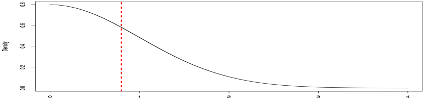
(a) $\phi$: half-normal, $m^{*}$: mean

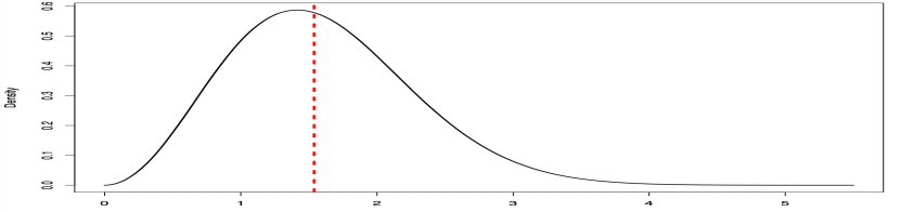
(b) $\phi$: Maxwell, $m^{*}$: median

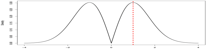
(c) $\phi$: double Rayleigh, $m^{*}$: right mode

Figure C.1: Plots of $\phi$ for Ex 3–Ex 5. The choices of $m^{*}$ are indicated in red dashed lines.

Ex 3. (Half-normal with the mean as the pivotal point): Let $\phi$ be the half-normal density (with scale 1). We set $n=700$, $\kappa=0.1$, $m^{*}$ as the mean, $\nu^{*}=0.1$ and $\sigma^{*}=0.2,0.3,0.4$.

Ex 4. (Maxwell-Boltzmann with the median as the pivotal point): Here, $\phi$ is the Maxwell-Boltzmann density which is widely used in statistical mechanics (Huang,, 2008). We set $n=500$, $\kappa=0.2$, $m^{*}$ as the median, $\nu^{*}=0.1$ and $\sigma^{*}=0.4,0.5,0.6$.

Ex 5. (Double Rayleigh with $m^{*}$ as the right mode): Let $\phi$ be the double Rayleigh density (with scale 1), $n=500$, $\kappa=0.1$, $m^{*}$ be the right mode, $\nu^{*}=0.1$ and $\sigma^{*}=0.2,0.3,0.4$.

Skewed half-normal
		$\sigma^{*}/\nu^{*}=2$				$\sigma^{*}/\nu^{*}=3$				$\sigma^{*}/\nu^{*}=4$
		Err($\beta$)	Err($\sigma$)	Err($\nu$)		Err($\beta$)	Err($\sigma$)	Err($\nu$)		Err($\beta$)	Err($\sigma$)	Err($\nu$)
QR∗		0.80	—	—		0.80	—	—		0.80	—	—
BQR∗		0.80	0.49	0.62		0.80	0.51	0.64		0.80	0.53	0.65
AME		0.64	0.99	1.22		0.56	1.0	2.02		0.48	1.0	2.82
ZQR		0.65	0.97	0.09		0.59	0.95	0.37		0.52	0.95	0.67
SPEUS		0.14	0.11	0.1		0.08	0.08	0.13		0.06	0.09	0.17
Skewed Maxwell-Boltzmann
		$\sigma^{*}/\nu^{*}=4$				$\sigma^{*}/\nu^{*}=5$				$\sigma^{*}/\nu^{*}=6$
		Err($\beta$)	Err($\sigma$)	Err($\nu$)		Err($\beta$)	Err($\sigma$)	Err($\nu$)		Err($\beta$)	Err($\sigma$)	Err($\nu$)
QR∗		1.59	—	—		1.59	—	—		1.59	—	—
BQR∗		1.59	0.41	0.74		1.59	0.43	0.75		1.59	0.44	0.75
AME		1.47	0.22	0.78		1.46	0.19	0.84		1.46	0.17	0.91
ZQR		1.49	0.58	0.30		1.48	0.58	0.32		1.48	0.57	0.34
SPEUS		0.18	0.14	0.20		0.17	0.13	0.21		0.16	0.12	0.30
Skewed double Rayleigh
		$\sigma^{*}/\nu^{*}=2$				$\sigma^{*}/\nu^{*}=3$				$\sigma^{*}/\nu^{*}=4$
		Err($\beta$)	Err($\sigma$)	Err($\nu$)		Err($\beta$)	Err($\sigma$)	Err($\nu$)		Err($\beta$)	Err($\sigma$)	Err($\nu$)
QR∗		1.0	—	—		1.0	—	—		1.0	—	—
BQR∗		1.0	0.68	0.27		1.0	0.70	0.26		1.0	0.71	0.26
AME		0.87	1.78	1.76		0.88	2.02	1.9		0.89	2.15	1.92
ZQR		0.67	0.50	1.67		0.50	0.48	2.69		0.32	0.45	3.78
SPEUS		0.22	0.03	0.18		0.15	0.03	0.24		0.10	0.03	0.26

Table C.1: Performance comparison for skewed half-normal with pivotal point at the mean, skewed Maxwell with pivotal point at the median, and skewed double Rayleigh with pivotal point at the right mode (Ex 3–Ex 5)

Table C.1 illustrates significant issues with conventional methods in capturing skewness, even when asymmetry is centered around the median, mean, or mode. Specifically, QR^∗ and BQR^∗ failed to accurately recover the true $\beta^{*}$ despite using the true quantile as input. Moreover, in all three cases, AME or AME provided at least one misleading estimate of the scales. In contrast, our proposed method demonstrated remarkable performance, with the associated $\beta$-error being at most $1/3$ of that of the other methods.

We also conducted experiments on the air pollution data of Leeds from 1994 to 1998 (Heffernan and Tawn,, 2004; Southworth et al.,, 2020). The dataset contain 578 measurements of the daily maximum levels of ozone (O3), nitrogen dioxide (NO2), nitrogen oxide (NO), sulfur dioxide (SO2) and particulate matter (PM10). We forecasted PM10 levels for the summer months (April to July) using other air pollutants. We considered the Gumbel model and its skewed pivot-blend enhancement SPEUS, in addition to ZQR, AME, and ESN. The p-values from the Kolmogorov-Smirnov tests for these models were 8e-2, 0.71, 9e-2, 0.20, and 8e-8, respectively. The results may appear surprising, considering the popularity of the skewed Gumbel distribution for modeling such extreme values (Boldi and Davison,, 2007). Figure C.2 presents the residual Q-Q plots, demonstrating that our skew-reinforced method significantly improves data fit compared to the classical Gumbel model.

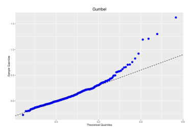
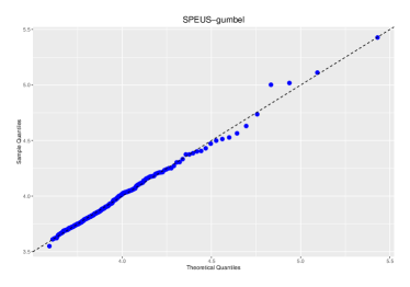
Figure C.2: Q-Q plots of residuals for Gumbel (left) and SPEUS (right) on air pollution data.

In real-world applications, data scientists frequently confront challenges related to skewness. However, fitting a common distribution that inadequately addresses these distortions can lead to subpar model fits and misleading inferences. The skewed pivot-blend technique refines skewness management in these distributions, thus enhancing the accuracy and reliability of the models.

References

• Agency for Healthcare Research and Quality, (2015) Agency for Healthcare Research and Quality (2015). MEPS HC-181: 2015 Full Year Consolidated Data File.
• Agency for Healthcare Research and Quality, (2019) Agency for Healthcare Research and Quality (2019). MEPS HC-216: 2019 Full Year Consolidated Data File.
• Arellano-Valle et al., (2005) Arellano-Valle, R. B., Gómez, H. W., and Quintana, F. A. (2005). Statistical inference for a general class of asymmetric distributions. Journal of Statistical Planning and Inference, 128(2):427–443.
• Axon and Kamel, (2021) Axon, D. R. and Kamel, A. (2021). Patterns of healthcare expenditures among older United States adults with pain and different perceived health status. Healthcare, 9(10):1327.
• Azzalini, (1985) Azzalini, A. (1985). A class of distributions which includes the normal ones. Scandinavian Journal of Statistics, 171–178.
• Azzalini, (2005) Azzalini, A. (2005). The skew-normal distribution and related multivariate families. Scandinavian Journal of Statistics, 32(2):159–188.
• Bartlett et al., (2019) Bartlett, P. L., Harvey, N., Liaw, C., and Mehrabian, A. (2019). Nearly-tight VC-dimension and pseudo-dimension bounds for piecewise linear neural networks. The Journal of Machine Learning Research, 20(1):2285–2301.
• Benoit and Van den Poel, (2017) Benoit, D. F. and Van den Poel, D. (2017). bayesQR: A Bayesian approach to quantile regression. Journal of Statistical Software, 76(1):1–32.
• Bera et al., (2016) Bera, A. K., Galvao, A. F., Montes-Rojas, G. V., and Park, S. Y. (2016). Asymmetric Laplace regression: Maximum likelihood, maximum entropy and quantile regression. Journal of Econometric Methods, 5(1):79–101.
• Bernardi and Bernardi, (2018) Bernardi, A. and Bernardi, M. (2018). Two-sided skew and shape dynamic conditional score models. Mathematical and Statistical Methods for Actuarial Sciences and Finance, pages 121–124.
• Bickel et al., (2009) Bickel, P. J., Ritov, Y., and Tsybakov, A. B. (2009). Simultaneous analysis of Lasso and Dantzig selector. The Annals of Statistics, 37(4):1705–1732.
• Boldi and Davison, (2007) Boldi, M. O. and Davison, A. C. (2007). A mixture model for multivariate extremes. Journal of the Royal Statistical Society: Series B (Statistical Methodology), 69(2):217–229.
• Boos, (1987) Boos, D. D. (1987). Detecting skewed errors from regression residuals. Technometrics, 29(1):83–90.
• Bregman, (1967) Bregman, L. M. (1967). The relaxation method of finding the common point of convex sets and its application to the solution of problems in convex programming. USSR Computational Mathematics and Mathematical Physics, 7(3):200–217.
• Chai and Bailey, (2008) Chai, H. S. and Bailey, K. R. (2008). Use of log-skew-normal distribution in analysis of continuous data with a discrete component at zero. Statistics in Medicine, 27(18):3643–3655.
• Chang and Joe, (2019) Chang, B. and Joe, H. (2019). Prediction based on conditional distributions of vine copulas. Computational Statistics $\&$ Data Analysis, 139:45–63.
• Cooray and Ananda, (2005) Cooray, K. and Ananda, M. M. (2005). Modeling actuarial data with a composite lognormal-pareto model. Scandinavian Actuarial Journal, 2005(5):321–334.
• Cragg, (1971) Cragg, J. G. (1971). Some statistical models for limited dependent variables with application to the demand for durable goods. Econometrica: Journal of the Econometric Society, 829–844.
• Devroye et al., (1996) Devroye, L., Györfi, L., and Lugosi, G. (1996). A Probabilistic Theory of Pattern Recognition. New York: Springer.
• Dominicy and Sinner, (2017) Dominicy, Y. and Sinner, C. (2017). Distributions and composite models for size-type data. In Hokimoto, T., editor, Advances in Statistical Methodologies and Their Application to Real Problems, chapter 8, pages 159–183. IntechOpen, Rijeka, Croatia.
• Fernández and Steel, (1998) Fernández, C. and Steel, M. F. (1998). On Bayesian modeling of fat tails and skewness. Journal of the American Statistical Association, 93(441):359–371.
• Giné and Nickl, (2015) Giné, E. and Nickl, R. (2015). Mathematical Foundations of Infinite-Dimensional Statistical Models. Cambridge: Cambridge University Press.
• Gitman et al., (2018) Gitman, I., Chen, J., Lei, E., and Dubrawski, A. (2018). Novel prediction techniques based on clusterwise linear regression. arXiv preprint:1804.10742.
• Goldberg and Jerrum, (1995) Goldberg, P. W. and Jerrum, M. R. (1995). Bounding the Vapnik-Chervonenkis dimension of concept classes parameterized by real numbers. Machine Learning, 18(2-3):131–148.
• Götze et al., (2021) Götze, F., Sambale, H., and Sinulis, A. (2021). Concentration inequalities for polynomials in $\alpha$-sub-exponential random variables. Electronic Journal of Probability, 26:1–22.
• Hampel et al., (2011) Hampel, F. R., Ronchetti, E. M., Rousseeuw, P. J., and Stahel, W. A. (2011). Robust Statistics: The Approach Based on Influence Functions. New Jersey: John Wiley & Sons.
• Heffernan and Tawn, (2004) Heffernan, J. E. and Tawn, J. A. (2004). A conditional approach for multivariate extreme values. Journal of the Royal Statistical Society: Series B (Statistical Methodology), 66(3):497–546.
• Hettmansperger and McKean, (1978) Hettmansperger, T. P. and McKean, J. W. (1978). Statistical inference based on ranks. Psychometrika, 43(1):69–79.
• Hettmansperger and McKean, (2010) Hettmansperger, T. P. and McKean, J. W. (2010). Robust Nonparametric Statistical Methods. Florida: CRC Press.
• Holle et al., (2021) Holle, M., Wolff, T., and Herant, M. (2021). Trends in the concentration and distribution of health care expenditures in the US, 2001-2018. JAMA Network Open, 4(9):e2125179–e2125179.
• Huang, (2008) Huang, K. (2008). Statistical Mechanics. New Jersey: John Wiley & Sons.
• Hyndman and Grunwald, (2000) Hyndman, R. J. and Grunwald, G. K. (2000). Applications: Generalized additive modelling of mixed distribution Markov models with application to Melbourne’s rainfall. Australian $\&$ New Zealand Journal of Statistics, 42(2):145–158.
• Jaeckel, (1972) Jaeckel, L. A. (1972). Estimating regression coefficients by minimizing the dispersion of the residuals. The Annals of Mathematical Statistics, 43(5):1449–1458.
• Jones, (2014) Jones, M. (2014). Generating distributions by transformation of scale. Statistica Sinica, 749–771.
• Klugman et al., (2012) Klugman, S. A., Panjer, H. H., and Willmot, G. E. (2012). Loss models: from data to decisions, volume 715. John Wiley & Sons.
• Koenker, (2009) Koenker, R. (2009). Package ‘quantreg’. http://CRAN.R-project.org/package=quantreg.
• Koenker and Bassett Jr, (1978) Koenker, R. and Bassett Jr, G. (1978). Regression quantiles. Econometrica: Journal of the Econometric Society, 33–50.
• Kottas and Gelfand, (2001) Kottas, A. and Gelfand, A. E. (2001). Bayesian semiparametric median regression modeling. Journal of the American Statistical Association, 96(456):1458–1468.
• Kuchibhotla and Chakrabortty, (2022) Kuchibhotla, A. K. and Chakrabortty, A. (2022). Moving beyond sub-Gaussianity in high-dimensional statistics: Applications in covariance estimation and linear regression. Information and Inference: A Journal of the IMA, 11:1389–1456.
• Lambert, (1992) Lambert, D. (1992). Zero-inflated Poisson regression, with an application to defects in manufacturing. Technometrics, 34(1):1–14.
• Lee, (1989) Lee, M. J. (1989). Mode regression. Journal of Econometrics, 42(3):337–349.
• Linero et al., (2020) Linero, A. R., Sinha, D., and Lipsitz, S. R. (2020). Semiparametric mixed-scale models using shared Bayesian forests. Biometrics, 76(1):131–144.
• Liu et al., (2008) Liu, L., Ma, J. Z., and Johnson, B. A. (2008). A multi-level two-part random effects model, with application to an alcohol-dependence study. Statistics in Medicine, 27(18):3528–3539.
• Ma and Genton, (2004) Ma, Y. and Genton, M. G. (2004). Flexible class of skew-symmetric distributions. Scandinavian Journal of Statistics, 31(3):459–468.
• Maronna et al., (2006) Maronna, R. A., Martin, D. R., and Yohai, V. J. (2006). Robust Statistics: Theory and Methods. New Jersey: John Wiley & Sons.
• Mudholkar and Hutson, (2000) Mudholkar, G. S. and Hutson, A. D. (2000). The epsilon-skew-normal distribution for analyzing near-normal data. Journal of Statistical Planning and Inference, 83(2):291–309.
• Mullahy, (1998) Mullahy, J. (1998). Much ado about two: Reconsidering retransformation and the two-part model in health econometrics. Journal of Health Economics, 17(3):247–281.
• Nadarajah and Kotz, (2003) Nadarajah, S. and Kotz, S. (2003). Skewed distributions generated by the normal kernel. Statistics $\&$ Probability Letters, 65(3):269–277.
• Nash et al., (1994) Nash, W. J., Sellers, T. L., Talbot, S. R., Cawthorn, A. J., and Ford, W. B. (1994). The population biology of abalone (Haliotis species) in Tasmania. i. blacklip abalone (H. rubra) from the North Coast and islands of Bass Strait. Sea Fisheries Division, Technical Report, 48:411.
• Olsen and Schafer, (2001) Olsen, M. K. and Schafer, J. L. (2001). A two-part random-effects model for semicontinuous longitudinal data. Journal of the American Statistical Association, 96(454):730–745.
• Rubio and Steel, (2020) Rubio, F. J. and Steel, M. F. (2020). The family of two-piece distributions. Significance, 17(1):12–13.
• Rubio and Steel, (2015) Rubio, F. J. and Steel, M. F. J. (2015). Bayesian modelling of skewness and kurtosis with two-piece scale and shape distributions. Electronic Journal of Statistics, 9(2):1884–1912.
• Sambale, (2020) Sambale, H. (2020). Some notes on concentration for $\alpha$-subexponential random variables. arXiv preprint:2002.10761.
• Sarul and Sahin, (2015) Sarul, L. S. and Sahin, S. (2015). An application of claim frequency data using zero inflated and hurdle models in general insurance. Journal of Business Economics and Finance, 4(4).
• Scollnik, (2007) Scollnik, D. (2007). On composite lognormal-Pareto models. Scandinavian Actuarial Journal, 2007(1):20–33.
• She, (2016) She, Y. (2016). On the finite-sample analysis of $\Theta$-estimators. Electronic Journal of Statistics, 10:1874–1895.
• She and Tran, (2019) She, Y. and Tran, H. (2019). On cross-validation for sparse reduced rank regression. Journal of the Royal Statistical Society: Series B (Statistical Methodology), 81(1):145–161.
• She et al., (2021) She, Y., Wang, Z., and Jin, J. (2021). Analysis of generalized bregman surrogate algorithms for nonsmooth nonconvex statistical learning. The Annals of Statistics, 49(6):3434–3459.
• Southworth et al., (2020) Southworth, H., Heffernan, J. E., and Metcalfe, P. (2020). Package ‘texmex’. https://cran.r-project.org/package=texmex.
• Stacy, (1962) Stacy, E. W. (1962). A generalization of the Gamma distribution. The Annals of Mathematical Statistics, 33(3):1187–1192.
• Tarbath, (1999) Tarbath, D. (1999). Estimates of Growth and Natural Mortality of the Blacklip Abalone (Haliotis Rubra) in Tasmania. Technical report series. Tasmanian Aquaculture and Fisheries Institute.
• Tobin, (1958) Tobin, J. (1958). Estimation of relationships for limited dependent variables. Econometrica: Journal of the Econometric Society, 24–36.
• van de Geer and Bühlmann, (2009) van de Geer, S. A. and Bühlmann, P. (2009). On the conditions used to prove oracle results for the Lasso. Electronic Journal of Statistics, 3:1360–1392.
• van der Vaart and Wellner, (2013) van der Vaart, A. W. and Wellner, J. A. (2013). Weak Convergence and Empirical Processes: With Applications to Statistics. Berlin: Springer Science & Business Media.
• Wainwright, (2019) Wainwright, M. J. (2019). High-dimensional Statistics: A Non-Asymptotic Viewpoint. Cambridge: Cambridge University Press.
• Wang et al., (2004) Wang, J., Boyer, J., and Genton, M. G. (2004). A skew-symmetric representation of multivariate distributions. Statistica Sinica, 1259–1270.
• Wang et al., (2020) Wang, L., Peng, B., Bradic, J., Li, R., and Wu, Y. (2020). A tuning-free robust and efficient approach to high-dimensional regression. Journal of the American Statistical Association, 115(532):1700–1714.
• Yang et al., (2019) Yang, T., Gallagher, C. M., and McMahan, C. S. (2019). A robust regression methodology via M-estimation. Communications in Statistics-Theory and Methods, 48(5):1092–1107.
• Yu and Moyeed, (2001) Yu, K. and Moyeed, R. A. (2001). Bayesian quantile regression. Statistics $\&$ Probability Letters, 54(4):437–447.
• Zhu and Zinde-Walsh, (2009) Zhu, D. and Zinde-Walsh, V. (2009). Properties and estimation of asymmetric exponential power distribution. Journal of Econometrics, 148(1):86–99.