Theoretical research on low-frequency drift Alfvén waves in general Tokamak equilibria

Abstract

We developed kinetic models based on general fishbone-like dispersion relations. Firstly, a general model for arbitrary magnetic configuration and ion orbit width is presented. Then, by disregarding ion orbit width and approximating the magnetic geometry as circular, we introduce a simplified model that fully incorporates circulating/trapped ion effects. Finally, by considering the limit of ions being well-circulating or deeply trapped, the results directly revert to those observed in earlier theoretical studies.

1. Southwestern Institute of Physics, PO Box 432, Chengdu 610041, People’s Republic of China

2. Consorzio CREATE. Via Claudio, 21 80125 Napoli, Italy

leeyang_swip@outlook.com

1 Introduction

Alfvén waves and energetic particles, resulted from fusion reaction and auxiliary heating, are crucial to the performance of Tokamak devices. The theoretical research on low frequency drift Alfvén waves (DAW) is based on the general fishbone-like dispersion relation (GFLDR) [1, 2, 3] and gyrokinetic theory[4, 5]. Besides recovering diverse limits of the kinetic magnetohydrodynamic (MHD) energy principle, the GFLDR approach is also applicable to electromagnetic fluctuations, which exhibit a wide spectrum of spatial and temporal scales consistent with gyrokinetic descriptions of both the core and supra-thermal plasma components. Formally ,the GFLDR can be written as

$$i\Lambda=\delta W_{f}+\delta W_{k},$$ (1)

where $\Lambda$ is the generalized inertia, and $\delta W_{f}$ and $\delta W_{k}$ are, respectively, fluid and kinetic potential energy of electromagnetic fluctuations. In previous researches, $\Lambda$ is calculated with fluid[6] and kinetic approaches[7]. Furthermore, analytical findings regarding mode frequency, damping, and the impacts of finite orbit width can be corroborated through numerical verification, demonstrating a high level of agreement for both SAW continuum structure [8, 9, 10, 11] and and geodesic acoustic mode (GAM) oscillations[12, 13]. As a result, the GFLDR, serving as a useful theoretical framework, aids in comprehending experimental observations, numerical simulations, and analytical outcomes across varying degrees of approximation.

In the original theoretical works[14, 15] on DAW, ions considered in the kinetic analysis are assumed to be well circulating. Later on, the kinetic analysis was extended by including the deeply trapped ions and electrons[7, 16]. Moreover, the researches mentioned above are all based on the $s-\alpha$ model in Tokamak plasmas with circular configuration. However, the effects of general magnetic geometry and full circulating/trapped particles are not included in previous researches. Especially, the particles near circulating/trapped separatrix are not included in the previous theoretical models. In order to obtain a better understanding of experimental observations[17, 18] and provide a more precise kinetic model for theoretical researches[19], we need to include the general magnetic geometry and full orbit effects without assuming well-circulating/deeply-trapped ions and small ion orbit width.

In this work, we present a kinetic model with general magnetic geometry and arbitrary ion orbit width. With this general model, one can solve the problem of DAW in the inertial layer numerically as long as the guiding center orbit information is provided. By taking small ion orbit width limit and applying the $s-\alpha$ model, a simplified mode with full circulating/trapped ions effects is obtained. The generalized inertia with the modification of neoclassical effects can also be calculated with appropriate circular geometry data. Furthermore, if we assume ions are well circulating or deeply trapped, the results go back to those of the previous researches[7].

The rest of the paper is organized as follows. In Section 2, we present our general kinetic model including guiding center motion in general geometry, kinetic equation in ballooning space and governing equations. Section 3 is devoted to solve the governing equation of the general model inertial layer. A simplified model including the full circulating/trapped ions effects is presented in Section 4 for circular magnetic geometry by assuming small ion orbit width. Finally, the results are summarized and discussed in Section 5.

2 Theoretical model

2.1 Guiding center motion

The guiding center motion of single particles can be given as

$$\dot{\bm{X}_{s}}=v_{\parallel}\bm{b}+\frac{v_{\parallel}}{\Omega_{s}}\nabla\times\left(\bm{b}v_{\parallel}\right),$$ (2)

where $v_{\parallel}$ is the velocity parallel to magnetic field, $\Omega_{s}=e_{s}B/m_{s}c$ is the gyro-frequency of the s-species and $\bm{b}$ is the unit vector of magnetic field. In general model, the magnetic field configuration of 2-D asymmetric equilibrium can be denoted by the straight field aligned flux $\left(\psi,\theta,\zeta\right)$, where $\psi$ is the poloidal flux, $\theta$ is the poloidal angle, $\zeta=\phi-\nu\left(\psi,\theta\right)$, $\phi$ is the geometric toroidal angle and $\nu$ is a periodic function in $\theta$. Thus, the magnetic field is given as

$$\bm{B}_{0}=F\left(\psi\right)\nabla\phi+\nabla\phi\times\nabla\psi.$$ (3)

The safety factor can be defined as $q\left(\psi\right)=\bm{B}_{0}\cdot\nabla\zeta/\bm{B}_{0}\cdot\nabla\theta$ and the Jacobian ${\cal J}=\left(\nabla\psi\times\nabla\theta\cdot\nabla\zeta\right)^{-1}$. Then the particle orbit in the flux coordinates can be given as

$$\dot{\psi}_{s}=\dot{\bm{X}_{s}}\cdot\nabla\psi=-\frac{v_{\parallel}}{{\cal J}B}\frac{\partial\bar{\psi}_{s}}{\partial\theta},$$ (4)

$$\dot{\theta}_{s}=\dot{\bm{X}_{s}}\cdot\nabla\theta=\frac{v_{\parallel}}{{\cal J}B}\frac{\partial\bar{\psi}_{s}}{\partial\psi},$$ (5)

$$\dot{\zeta_{s}}=\dot{\bm{X}_{s}}\cdot\nabla\zeta=\frac{qv_{\parallel}}{{\cal J}B}+\frac{v_{\parallel}m_{s}c}{{\cal J}Be_{s}}\left[\frac{\partial}{\partial\psi}\left({\cal J}B_{0}v_{\parallel}-q\frac{Fv_{\parallel}}{B}\right)+\frac{\partial}{\partial\theta}\left({\cal J}v_{\parallel}\frac{\nabla\psi\cdot\nabla\theta}{BR^{2}}-\frac{Fv_{\parallel}}{B}\frac{\partial\nu}{\partial\psi}\right)\right],$$ (6)

where $R=\left|\nabla\phi\right|^{-1}$ and $\bar{\psi}_{s}=\psi-Fv_{\parallel}/\Omega_{s}$. As we can see, $\bar{\psi}_{s}$ is a constant along the particle orbit. In order to study the responses of trapped and circulating particles, the canonical angle can be introduced as[20]

$$\vartheta_{c}=\omega_{bs}\int^{\vartheta_{0}}\frac{d\vartheta_{0}^{\prime}}{\dot{\theta}_{s}},$$ (7)

where the bouncing frequency $\omega_{bs}=2\pi/\left(\ointclockwise d\vartheta_{0}/\dot{\theta_{s}}\right)$, and $\ointclockwise$ means the integration along the particle orbit with constant $\bar{\psi}_{s}$.

2.2 Kinetic equation in ballooning space

Before going to ballooning space, we start the analysis from the gyro-kinetic equation in original space. The perturbed particle distribution function can be written as[5, 1]

$$\delta f_{s}=\left(\frac{e}{m}\right)_{s}\left[\frac{\partial F_{0}}{\partial{\cal E}}\delta\phi-J_{0}\left(k_{\perp}\rho_{Ls}\right)\frac{QF_{0}}{\omega}\delta\psi e^{iL_{k}}\right]_{s}+\delta K_{s}e^{iL_{ks}},$$ (8)

where $\delta\phi$ is perturbed electric potential, $\delta\psi$ is related to parallel vector potential fluctuation $\delta A_{\parallel}$ with $\delta A_{\parallel}=-i\left(\frac{c}{\omega}\right)\bm{b}\cdot\nabla\delta\psi$, $k_{\perp}^{2}=k^{2}-\left(\bm{k}\cdot\bm{b}\right)^{2}$, $J_{0}$ is the 0th Bessel function, $\rho_{Ls}=m_{s}cv_{\perp}/e_{s}B_{0}$ the Lamor radius, $QF_{0s}=\left[\omega\partial_{{\cal E}}+\Omega_{s}^{-1}\left(\bm{k}\times\bm{b}\right)\cdot\nabla\right]F_{0s}$, and $L_{ks}=\left(m_{s}c/e_{s}B_{0}\right)\left(\bm{k}\times\bm{b}\right)\cdot\bm{v}$. And the non-adiabatic part $\delta K_{s}$ obeys the gyro-kinetic equation as

$$\left(-i\omega+\dot{\psi}\partial_{\psi}+\dot{\theta}\partial_{\theta}+\dot{\zeta}\partial_{\zeta}\right) \delta K_{s}=i\left(\frac{e}{m}\right)_{s}QF_{0s}\times$$

$$\left[J_{0}\left(\delta\phi-\delta\psi\right)+\left(\frac{\omega_{d}}{\omega}\right)_{s}J_{0}\delta\psi+\frac{v_{\perp}}{k_{\perp}c}J_{1}\delta B_{\parallel}\right],$$ (9)

where $J_{1}$ is the 1st Bessel function, $\omega_{ds}=\left(\bm{k}\times\bm{b}\right)\cdot\left(\mu\nabla B_{0}+v_{\parallel}^{2}\bm{\kappa}\right)/\Omega_{s}$, $\bm{\kappa}$ is the curvature of magnetic field line and $\delta B_{\parallel}$ is the perturbed parallel magnetic field. By considering the ballooning representation, we have[1]

$$f\left(\psi,\theta,\zeta\right) =e^{in\zeta}\sum_{m}e^{-im\theta}f_{m,n}$$

$$=e^{in\zeta}\sum_{m}e^{-im\theta}\int e^{-i\left(nq-m\right)\vartheta}\hat{f}d\vartheta.$$ (10)

Then the gyro-kinetic equation (9) can be rewritten as

$$\left[-i\omega+\dot{\theta}\partial_{\vartheta}+i\omega_{ds}\right] \delta\hat{K}_{s}=i\left(\frac{e}{m}\right)_{s}QF_{0s}$$

$$\times \left[J_{0}\left(\delta\phi-\delta\psi\right)+\frac{\omega_{ds}}{\omega}J_{0}\delta\psi+\frac{v_{\perp}}{k_{\perp}c}J_{1}\delta B_{\parallel}\right],$$ (11)

where $\omega_{ds}=-nq^{\prime}\dot{\psi}_{s}\vartheta+n\left(\dot{\zeta}_{s}-q\dot{\theta}_{s}\right)$ in ballooning representation. For the simplicity of notation, $\omega_{ds}$ denotes the drift frequency in ballooning space. Before further analysis, it should be noted that the analysis in this work will be carried out in the inertial layer. Thus, we have two scales, i.e. $\left|\vartheta_{1}\right|\sim\delta^{-1}\sim\beta^{-1/2}$ and $\left|\vartheta_{0}\right|\sim 1$, where $\delta$ is the small parameter. In the original space , $\dot{\theta}_{s}$, $\dot{\zeta}_{s}$ and $\dot{\psi}_{s}$ are all periodic functions in $\theta$. Since periodic function in $\theta$ and be represented as periodic function in $\vartheta$, all the periodic functions in original space, can be treated as functions only in the short scale $\vartheta_{0}$, which indicates that the particle orbit is on the scale of $\vartheta_{0}$.

2.3 Governing equations

The governing equations for low frequency AE problem include mainly vorticity equation and quasi-neutrality equation. Formally, the vorticity equation can be given as[21]

$$\text{FLB}+\text{ICU}+\text{MPC}+\text{KPC}+\text{MFC}=0,$$ (12)

where FLB is finite line bending term, ICU is inertia-charge uncovering term, MPC is MHD non-adiabatic particle compression term. KPC is kinetic particle compression term, MFC is magnetic field compression. And these terms can be expressed as

$$\text{FLB}\simeq\bm{B}\cdot\nabla\left(\frac{k_{\perp}^{2}}{k_{\vartheta}^{2}B^{2}}\bm{B}\cdot\nabla\delta\hat{\psi}\right)=\frac{1}{{\cal J}}\partial_{\vartheta}\left(\frac{k_{\perp}^{2}}{{\cal J}k_{\vartheta}^{2}B_{0}^{2}}\partial_{\vartheta}\delta\hat{\psi}\right),$$ (13)

ICU $$\simeq-\frac{4\pi\omega^{2}}{k_{\vartheta}^{2}c^{2}}\sum_{s}\left\langle\frac{e_{s}^{2}}{m_{s}}\frac{QF_{0s}}{\omega}\left(1-J_{0}^{2}\right)\delta\hat{\phi}\right\rangle,$$ (14)

$$\text{MPC}=\frac{4\pi}{k_{\vartheta}^{2}c^{2}}\sum_{s}\frac{e_{s}^{2}}{m_{s}}\left\langle J_{0}^{2}\omega\omega_{ds}\frac{QF_{0s}}{\omega}\delta\hat{\phi}\right\rangle_{v},$$ (15)

$$\text{KPC}=-\sum_{s}\frac{4\pi e_{s}}{k_{\vartheta}^{2}c^{2}}\left\langle J_{0}\omega\omega_{ds}\delta K_{s}\right\rangle_{v},$$ (16)

$$\text{MFC}=\frac{4\pi\omega^{2}}{k_{\vartheta}^{2}c^{2}}\sum_{s}\left\langle\frac{v_{\perp}}{k_{\perp}c}J_{0}J_{1}\frac{e_{s}^{2}}{m_{s}}\frac{QF_{0s}}{\omega}\delta\hat{B}_{\parallel}\right\rangle_{v},$$ (17)

where $\left\langle\cdots\right\rangle_{v}=2\pi\sum_{\sigma}\int\int B/\left|v_{\parallel}\right|\left(\cdots\right)d{\cal E}d\mu$ . Here we have assumed $F_{0s}$s are isotropic in pitch angle and used the parallel Ampère’s law

$$\frac{k_{\perp}^{2}}{k_{\vartheta}^{2}}\bm{b}\cdot\nabla\delta\psi=\frac{4\pi}{k_{\vartheta}^{2}c^{2}}i\omega\sum_{s}e_{s}\left\langle v_{\parallel}\delta f_{s}\right\rangle_{v},$$ (18)

and perpendicular Ampère’s law

$$\delta B_{\parallel}\simeq\frac{4\pi}{B^{2}}\frac{c}{\omega}\left(\bm{k}\times\bm{b}\cdot\nabla P_{\perp}\right)\delta\psi,$$ (19)

where $P_{\perp}=P_{\perp i}+P_{\perp e}$ is the total perpendicular pressure. By re-defining $\left[\delta\Psi,\delta\Phi,\delta\hat{B}_{\parallel}\right]=\frac{k_{\perp}}{k_{\vartheta}}\left[\delta\psi,\delta\phi,\delta B_{\parallel}\right]=\hat{\kappa}_{\perp}\left[\delta\psi,\delta\phi,\delta B_{\parallel}\right]$ and considering $\hat{\kappa}_{\perp}\sim s\left|\vartheta_{1}\right|\sim\delta^{-1}$, the vorticity equation can be rewritten as

$$\left(\frac{\partial^{2}}{\partial\vartheta^{2}}-\frac{\partial_{\vartheta}^{2}\left|\nabla\psi\right|}{\left|\nabla\psi\right|}\right)\delta\Psi+\frac{{\cal J}^{2}B^{2}}{\hat{\kappa}_{\perp}}\left(\text{ICU}+\text{MPC}+\text{MFC}+\text{KPC}\right)=0.$$ (20)

Is should be noted that all the terms $\delta\psi$, $\delta\phi$ and $\delta B_{\parallel}$are substituted by $\delta\Psi$, $\delta\Phi$, and $\delta\hat{B}_{\parallel}$ respectively in Eq. (20). And the quasi-neutrality equation is

$$\sum_{s}\left\langle\delta f_{s}\right\rangle_{v}=0.$$ (21)

By solving the governing equations (19)-(21), the physical property of DAW in the inertial layer can be determined.

3 General solution in singular layer

In the singular layer with $\vartheta_{1}\sim\delta^{-1}$, we have the orderings $\delta\omega_{di}\sim\omega\sim\omega_{*Pi}\sim\omega_{bi}$ for circulating ions and $\omega_{de}\sim\omega_{di}\sim\omega\sim\omega_{bi}\sim\delta\omega_{be}$ for trapped ions and electrons, where $\omega_{*Pi}=\omega_{*Ti}+\omega_{*ni}$, $\omega_{*Ti}=\left(T_{i}c/e_{i}B\right)\left(\bm{k}\times\bm{b}\right)\cdot\left(\nabla T_{i}\right)/T_{i}$, $\omega_{*ni}=\left(T_{i}c/e_{i}B\right)\left(\bm{k}\times\bm{b}\right)\cdot\left(\nabla n_{i}\right)/n_{i}$, $T_{i}$ is the ion temperature and $n_{i}$ is the ion density. Moreover, the Lamor radius of ions is assumed to be small, i.e. $k_{\perp}\rho_{ti}\sim\delta$, in singular layer.

The 0th order kinetic equations for circulating ions, trapped ions and trapped electrons can be written as

$$\left(\dot{\vartheta}\partial_{\vartheta_{0}}-i\omega\right)\delta K_{cir}^{\left(0\right)}=i\left(\frac{e}{m}QF_{0}\right)_{i}\frac{k_{\vartheta}}{k_{\perp}}\left(\delta\Phi^{\left(0\right)}-\delta\Psi^{\left(0\right)}\right),$$ (22)

$$\left(\dot{\vartheta}\partial_{\vartheta_{0}}-i\omega+i\omega_{di}\right)\delta K_{tr,i}^{\left(0\right)}=i\left(\frac{e}{m}QF_{0}\right)_{i}\frac{k_{\vartheta}}{k_{\perp}}\left(\delta\Phi^{\left(0\right)}-\delta\Psi^{\left(0\right)}+\frac{\omega_{di}}{\omega}\delta\Psi^{\left(0\right)}\right),$$ (23)

$$\left(-i\omega+i\omega_{de}\right)\delta K_{tr,e}^{\left(0\right)}=i\left(\frac{e}{m}QF_{0}\right)_{e}\frac{k_{\vartheta}}{k_{\perp}}\left(\delta\Phi^{\left(0\right)}-\delta\Psi^{\left(0\right)}+\frac{\bar{\omega}_{de}}{\omega}\delta\Psi^{\left(0\right)}\right),$$ (24)

where

$$\bar{\omega}_{ds}=\frac{n\omega_{bs}}{2\pi}\ointclockwise\frac{\dot{\zeta_{s}}-q\dot{\theta_{s}}}{\dot{\theta_{s}}}d\vartheta_{0},$$ (25)

and $\delta K_{cir}^{\left(0\right)}$, $\delta K_{tr,i}^{(0)}$ and $\delta K_{tr,e}^{\left(0\right)}$ are, respectively, 0th order non-adiabatic kinetic responses for circulating ions, trapped ions and trapped electrons. As shown in the equations above, the solutions for $\delta K_{circ}^{\left(0\right)}$ and $\delta K_{tr,e}^{\left(0\right)}$ can be readily written as

$$\delta K_{cir}^{\left(0\right)}=-\left(\frac{e}{m}\right)_{i}\frac{QF_{0i}}{\omega}\frac{k_{\vartheta}}{k_{\perp}}\left(\delta\Phi^{\left(0\right)}-\delta\Psi^{\left(0\right)}\right),$$ (26)

and

$$\delta K_{tr,e}=-QF_{0e}\left(\frac{e}{m}\right)_{e}\frac{k_{\vartheta}/k_{\perp}}{\omega-\bar{\omega}_{de}}\left[\frac{\bar{\omega}_{de}}{\omega}\delta\Psi^{\left(0\right)}+\delta\Phi^{\left(0\right)}-\delta\Psi^{\left(0\right)}\right].$$ (27)

It should be noted that the solution (27) is obtained by neglecting the electron orbit width. By integrating over $\vartheta_{c}$ along particle orbit, the solution of Eq. (23) can be formally written as[20]

$$\delta K_{tr,i}^{\left(0\right)}= \frac{e^{-i\tilde{Q}_{b}}}{2\pi}\sum_{l}\frac{e^{il\vartheta_{c}}}{-i\omega+i\bar{\omega}_{di}+i\left(l-n\bar{q}\right)\omega_{bi}}\oint d\vartheta_{c}e^{i\tilde{Q}_{b}\left(\vartheta_{c}^{\prime}\right)-il\vartheta_{c}^{\prime}}$$

$$\times i\left(\frac{e}{m}QF_{0}\right)_{i}\frac{k_{\vartheta}}{k_{\perp}}\left(\delta\Phi^{\left(0\right)}-\delta\Psi^{\left(0\right)}+\frac{\omega_{di}}{\omega}\delta\Psi^{\left(0\right)}\right),$$ (28)

where

$$\tilde{Q}_{b}\left(\vartheta_{c}\right)=\tilde{\Xi}\left(\vartheta_{c}\right)-n\tilde{\Pi}\left(\vartheta_{c}\right)-n\vartheta_{1}\left[q\left(\vartheta_{c}\right)-q\left(0\right)\right],$$ (29)

$$\tilde{\Xi}=n\zeta\left(\vartheta_{c}\right)-\frac{\bar{\omega}_{di}}{\omega_{bi}}\vartheta_{c},$$ (30)

$$\tilde{\Pi}=\int^{\vartheta_{0}\left(\vartheta_{c}\right)}qd\vartheta_{0}-\vartheta_{c}\bar{q},$$ (31)

and $\bar{q}=\frac{1}{2\pi}\ointclockwise qd\vartheta_{0}$. As shown in Eq. (28), the resonance from toroidal and poloidal orbit frequency can be included by $\omega_{di}$ and $\omega_{bi}$. From Eq. (21), the 0th order quasi-neutrality equation can be given as

$$\left(1+\frac{1}{\tau}\right)\left(\delta\Phi^{\left(0\right)}-\delta\Psi^{\left(0\right)}\right)= \frac{T_{i}}{eN_{i}}\left\langle\frac{k_{\perp}}{k_{\vartheta}}\frac{1}{{\cal J}\omega_{bi}}\frac{\partial\bar{\psi_{i}}}{\partial\psi}\delta K_{circ}^{\left(0\right)}\right\rangle_{circ,\vartheta_{c}}$$

$$-\frac{T_{i}}{eN_{i}}\left\langle\frac{k_{\perp}}{k_{\vartheta}}\frac{1}{{\cal J}\omega_{be}}\delta K_{tr,e}\right\rangle_{tr,\vartheta_{c}} +\frac{T_{i}}{eN_{i}}\left\langle\frac{k_{\perp}}{k_{\vartheta}}\frac{1}{{\cal J}\omega_{bi}}\frac{\partial\bar{\psi_{i}}}{\partial\psi}\delta K_{tr}^{\left(0\right)}\right\rangle_{tr,\vartheta_{c}},$$ (32)

where the averaged ion density $N_{i}=\left\langle\frac{F_{0i}}{{\cal J}\omega_{bi}}\frac{\partial\bar{\psi_{i}}}{\partial\psi}\right\rangle_{full,\vartheta_{c}}$, $\left\langle\cdots\right\rangle_{full,\vartheta_{c}}=\left\langle\cdots\right\rangle_{circ,\vartheta_{c}}+\left\langle\cdots\right\rangle_{tr,\vartheta_{c}}$ $\left\langle\cdots\right\rangle_{circ,\vartheta_{c}}=\sum_{\sigma}\int\int\oint\left(\cdots\right)d\vartheta_{c}d{\cal E}d\mu$ within the circulating domain of $\left({\cal E},\mu\right)$, $\left\langle\cdots\right\rangle_{tr,\vartheta_{c}}=\int\int\oint\left(\cdots\right)d\vartheta_{c}d{\cal E}d\mu$ the integration within the domain of trapped particles[22], $\sigma=v_{\parallel}/\left|v_{\parallel}\right|$ and the summation $\sum_{\sigma}$ is operated only on circulating particles with opposite directions around $\bar{\psi}_{s}$. It should be noted that integration $\oint\left(\cdots\right)d\vartheta_{c}$ is carried out surrounding the rational surface $\bar{\psi}_{0}=\bar{\psi}_{s}$. The 0th order vorticity equation is just

$$\partial_{\vartheta_{0}}^{2}\delta\Psi^{\left(0\right)}=0,$$ (33)

which gives the plain result that $\delta\Psi^{\left(0\right)}$ is independent of $\vartheta_{0}$. From the Eq. (32), we can have a formal relation

$$\delta\Phi^{\left(0\right)}=N_{0}\delta\Psi^{\left(0\right)},$$ (34)

where $N_{0}=D_{1}/D_{2}$,

$$D_{1} =\left(1+\frac{1}{\tau}\right)+\frac{T_{i}}{eN_{i}}\left\langle\frac{k_{\perp}}{k_{\vartheta}}\frac{\left(\frac{e}{m}QF_{0}\right)_{e}}{{\cal J}\omega_{be}}\frac{k_{\vartheta}/k_{\perp}}{\omega-\bar{\omega}_{de}}\left(\frac{\bar{\omega}_{de}}{\omega}-1\right)\right\rangle_{tr,\vartheta_{c}}$$

$$+\frac{T_{i}}{eN_{i}}\left\langle\frac{k_{\perp}}{k_{\vartheta}}\frac{1}{{\cal J}\omega_{bi}}\frac{\partial\bar{\psi_{i}}}{\partial\psi}\left(\frac{e}{m}\right)_{i}\frac{QF_{0i}}{\omega}\frac{k_{\vartheta}}{k_{\perp}}\right\rangle_{circ,\vartheta_{c}}$$

$$+\frac{T_{i}}{eN_{i}}\left\langle\frac{k_{\perp}}{k_{\vartheta}}\frac{\partial\bar{\psi_{i}}}{\partial\psi}\frac{e^{-i\tilde{Q}_{b}}}{2\pi{\cal J}\omega_{bi}}\sum_{l}e^{il\vartheta_{c}}\oint\frac{\left(\frac{e}{m}QF_{0}\right)_{i}\frac{k_{\vartheta}}{k_{\perp}}\left(\frac{\omega_{di}}{\omega}-1\right)e^{i\tilde{Q}_{b}\left(\vartheta_{c}^{\prime}\right)-il\vartheta_{c}^{\prime}}}{-\omega+\bar{\omega}_{di}+\left(l-n\bar{q}\right)\omega_{bi}}d\vartheta_{c}\right\rangle_{tr,\vartheta_{c}},$$ (35)

and

$$D_{2} =\left(1+\frac{1}{\tau}\right)\frac{T_{i}}{eN_{i}}\left\langle\frac{k_{\perp}}{k_{\vartheta}}\frac{\left(\frac{e}{m}QF_{0}\right)_{e}}{{\cal J}\omega_{be}}\frac{k_{\vartheta}/k_{\perp}}{\omega-\bar{\omega}_{de}}\right\rangle_{tr,\vartheta_{c}}$$

$$+\frac{T_{i}}{eN_{i}}\left\langle\frac{k_{\perp}}{k_{\vartheta}}\frac{1}{{\cal J}\omega_{bi}}\frac{\partial\bar{\psi_{i}}}{\partial\psi}\left(\frac{e}{m}\right)_{i}\frac{QF_{0i}}{\omega}\frac{k_{\vartheta}}{k_{\perp}}\right\rangle_{circ,\vartheta_{c}}$$

$$+\frac{T_{i}}{eN_{i}}\left\langle\frac{k_{\perp}}{k_{\vartheta}}\frac{\partial\bar{\psi_{i}}}{\partial\psi}\frac{e^{-i\tilde{Q}_{b}}}{2\pi{\cal J}\omega_{bi}}\sum_{l}e^{il\vartheta_{c}}\oint\frac{\left(\frac{e}{m}QF_{0}\right)_{i}\frac{k_{\vartheta}}{k_{\perp}}e^{i\tilde{Q}_{b}\left(\vartheta_{c}^{\prime}\right)-il\vartheta_{c}^{\prime}}}{-\omega+\bar{\omega}_{di}+\left(l-n\bar{q}\right)\omega_{bi}}d\vartheta_{c}\right\rangle_{tr,\vartheta_{c}}$$

As shown above, the ideal MHD condition, i.e. $\delta\Phi=\delta\Psi$, is modified by trapped particles. The 1st order vorticity equation is $\partial_{\vartheta_{0}}^{2}\delta\Psi^{\left(1\right)}=0$, which gives the result that $\delta\Psi^{\left(1\right)}=0$. And $\delta\Phi^{\left(1\right)}=\sum_{l}\delta\Phi_{l}e^{il\vartheta_{0}}$ in general. The 1st kinetic equation for circulating ions can be given as

$$\left(\omega_{b}\partial_{\vartheta_{c}}-i\omega\right)\delta K_{circ}^{\left(1\right)}=-\dot{\vartheta}\partial_{\vartheta_{1}}\delta K_{circ}^{\left(0\right)}+i\frac{k_{\vartheta}}{k_{\perp}}\left(\frac{e}{m}\right)QF_{0i}\left[\delta\Phi^{\left(1\right)}+\frac{\omega_{di}}{\omega}\delta\Phi^{\left(0\right)}\right].$$ (36)

The solution can be written as

$$\delta K_{circ}^{\left(1\right)}= -\sum_{l}\left(\frac{e}{m}\right)_{i}\frac{1}{\omega-l\omega_{bi}}\left(\frac{1}{2\pi}\sum_{l^{\prime}}\delta\Phi_{l^{\prime}}\oint\frac{k_{\vartheta}}{k_{\perp}}QF_{0i}e^{il^{\prime}\vartheta_{0}^{\prime}-il\vartheta_{c}^{\prime}}d\vartheta_{c}^{\prime}\right)e^{il\vartheta_{c}}$$

$$-\sum_{l}\frac{1}{\omega\left(\omega-l\omega_{bi}\right)}\left(\frac{e}{m}\right)_{i}\delta\Phi^{\left(0\right)}\left(\frac{1}{2\pi}\oint\frac{k_{\vartheta}}{k_{\perp}}QF_{0i}\omega_{di}e^{-il\vartheta_{c}^{\prime}}d\vartheta_{c}^{\prime}\right)e^{il\vartheta_{c}}$$

$$-\frac{i}{\omega}\partial_{\vartheta_{1}}\delta K_{circ}^{\left(0\right)}.$$ (37)

Then the 1st order quasi-neutrality of the l-th component can be cast as

$$\left(1+\frac{1}{\tau}\right)\delta\Phi_{l} =\frac{T_{i}}{eN_{i}}\left\langle\frac{k_{\perp}}{k_{\vartheta}}\frac{e^{-il\vartheta_{0}}}{{\cal J}\omega_{bi}}\frac{\partial\bar{\psi}_{i}}{\partial\psi}\delta K_{circ}^{\left(1\right)}\right\rangle_{circ,\vartheta_{c}}$$

$$+\frac{T_{i}}{eN_{i}}\left\langle\frac{k_{\perp}}{k_{\vartheta}}\frac{1-\delta_{l0}}{{\cal J}\omega_{bi}}e^{-il\vartheta_{0}}\frac{\partial\bar{\psi}_{i}}{\partial\psi}\delta K_{tr}^{\left(0\right)}\right\rangle_{tr,\vartheta_{c}},$$ (38)

where $1-\delta_{l0}$ is introduced to avoid the double-counting of the $l=0$ part of $\delta K_{tr}^{\left(0\right)}$ and $\delta_{l0}$ is the Kronecker symbol. If we cut off the harmonic to finite $l$, the Eqs. (34), (37) and (38) form a complete set of equations to give the relation

$$\delta\Phi_{l}=N_{l}\delta\Psi^{\left(0\right)},$$ (39)

where $N_{l}=M_{ll^{\prime}}^{-1}X_{l^{\prime}}$,

$$X_{l} =-\frac{T_{i}N_{0}}{eN_{i}}\left\langle\frac{k_{\perp}}{k_{\vartheta}}\frac{e^{il\vartheta_{c}-il\vartheta_{0}}}{{\cal J}\omega_{bi}}\frac{\partial\bar{\psi}_{i}}{\partial\psi}\sum_{l}\frac{\left(\frac{e}{m}\right)_{i}\left(\frac{1}{2\pi}\oint\frac{k_{\vartheta}}{k_{\perp}}QF_{0i}\omega_{di}e^{-il\vartheta_{c}^{\prime}}d\vartheta_{c}^{\prime}\right)}{\omega\left(\omega-l\omega_{bi}\right)}\right\rangle_{circ,\vartheta_{c}}$$

$$-\frac{iT_{i}}{eN_{i}\omega\delta\Psi^{\left(0\right)}}\left\langle\frac{k_{\perp}}{k_{\vartheta}}\frac{e^{-il\vartheta_{0}}}{{\cal J}\omega_{bi}}\frac{\partial\bar{\psi}_{i}}{\partial\psi}\partial_{\vartheta_{1}}\delta K_{circ}^{\left(0\right)}\right\rangle_{circ,\vartheta_{c}}\delta_{l0}$$

$$\frac{T_{i}}{eN_{i}\delta\Psi^{\left(0\right)}}\left\langle\frac{k_{\perp}}{k_{\vartheta}}\frac{1-\delta_{l0}}{{\cal J}\omega_{bi}}e^{-il\vartheta_{0}}\frac{\partial\bar{\psi}_{i}}{\partial\psi}\delta K_{tr}^{\left(0\right)}\right\rangle_{tr,\vartheta_{c}},$$

and

$$M_{ll^{\prime}} =\left(1+\frac{1}{\tau}\right)\delta_{ll^{\prime}}+\frac{T_{i}}{eN_{i}}\left\langle\frac{k_{\perp}}{k_{\vartheta}}\sum_{l^{\prime\prime}}\frac{e^{il^{\prime\prime}\vartheta_{c}-il\vartheta_{0}}}{{\cal J}\omega_{bi}}\frac{\partial\bar{\psi}_{i}}{\partial\psi}\left(\frac{e}{m}\right)_{i}\frac{\left(\frac{1}{2\pi}\oint\frac{k_{\vartheta}}{k_{\perp}}QF_{0i}e^{il^{\prime}\vartheta_{0}^{\prime}-il^{\prime\prime}\vartheta_{c}^{\prime}}d\vartheta_{c}^{\prime}\right)}{\omega-l^{\prime\prime}\omega_{bi}}\right\rangle_{circ,\vartheta_{c}}.$$ (40)

By averaging $\vartheta_{0}$, the 2nd order vorticity equation can be obtained as

$$\left(\frac{\partial^{2}}{\partial\vartheta_{1}^{2}}-\frac{1}{2\pi}\oint\frac{\partial_{\vartheta}^{2}\left|\nabla\psi\right|}{\left|\nabla\psi\right|}d\vartheta_{0}\right)\delta\Psi^{\left(0\right)}$$

$$+\frac{4\pi}{c^{2}}\sum_{s}\left\langle\frac{e_{s}^{2}}{m_{s}}{\cal J}B^{2}\frac{v_{\perp}\omega}{k_{\perp}^{2}\omega_{bs}}\frac{\partial\bar{\psi}_{s}}{\partial\psi}J_{0}J_{1}QF_{0s}\right\rangle_{full,\vartheta_{c}}\delta\hat{B}_{\parallel}^{\left(0\right)}$$

$$+\frac{4\pi}{c^{2}}\sum_{s}\frac{e_{s}^{2}}{m_{s}}\left\langle\frac{{\cal J}B^{2}}{k_{\perp}^{2}}J_{0}^{2}\frac{\omega_{ds}}{\omega_{bs}}\frac{\partial\bar{\psi}_{s}}{\partial\psi}QF_{0s}\right\rangle_{full,\vartheta_{c}}\delta\Psi^{\left(0\right)}$$

$$-\frac{4\pi N_{0}}{c^{2}}\sum_{s}\frac{e_{s}^{2}}{m_{s}}\left\langle\frac{{\cal J}B^{2}}{k_{\perp}^{2}}\frac{\omega}{\omega_{bs}}\left(1-J_{0}^{2}\right)\frac{\partial\bar{\psi}_{s}}{\partial\psi}QF_{0s}\right\rangle\delta\Psi^{\left(0\right)}$$

$$=\left\langle\frac{{\cal J}B^{2}}{\hat{\kappa}_{\perp}}\frac{4\pi e_{i}}{k_{\vartheta}^{2}c^{2}}\frac{\omega\omega_{di}}{\omega_{bi}}J_{0}\frac{\partial\bar{\psi}_{s}}{\partial\psi}\delta K_{circ}^{\left(1\right)}\right\rangle_{circ,\vartheta_{c}}$$

$$+\sum_{s}\left\langle\frac{{\cal J}B^{2}}{\hat{\kappa}_{\perp}}\frac{4\pi e_{s}}{k_{\vartheta}^{2}c^{2}}\frac{\omega\omega_{ds}}{\omega_{bs}}J_{0}\frac{\partial\bar{\psi}_{s}}{\partial\psi}\delta K_{tr,s}^{\left(0\right)}\right\rangle_{tr,\vartheta_{c}}.$$ (41)

Here for the leading order terms, $J_{0}^{2}\simeq 1$, $1-J_{0}^{2}\simeq k_{\perp}^{2}\rho_{Ls}^{2}/2$ and $J_{1}\simeq k_{\perp}\rho_{Ls}/2$. With Eqs. (26) , (27), (28), (32), (37) and (38), Eq. (41) can be solved, in general, numerically provided that the information of particle orbit on the grid of $\left({\cal E},\mu\right)$ and general magnetic geometry data are given numerically. In this general model, we can consider arbitrary magnetic configuration and ion orbit width[23].

4 An application to circular geometry

4.1 Reduced model

In this application, we will only consider the leading order solution without assuming well circulating and deeply trapped particles. For the circular up-down symmetric configuration, the magnetic field $B=B_{0}\left(1-\epsilon\cos\theta\right)$, where $\epsilon=r/R_{0}\sim\delta^{2}$ is the inverse aspect ratio. Also, ${\cal J}B_{0}^{2}\simeq qR_{0}B_{0}$, $\tilde{Q}_{b}\simeq 0$ and $\bar{\psi}_{s}\simeq\psi$ because of the small orbit width approximation. Thus, for trapped ions, $\bar{q}\simeq 0$. The guiding center motion is governed by

$$\dot{\theta_{s}}=\frac{v_{\parallel}}{qR_{0}},$$ (42)

$$\dot{\zeta_{s}}-q\dot{\theta_{s}}=\frac{q}{2rR_{0}\Omega_{s}}\left(v^{2}+v_{\parallel}^{2}\right)\cos\theta,$$ (43)

$$q^{\prime}\dot{\psi_{s}}\vartheta_{1}=\frac{q}{2rR_{0}\Omega_{s}}\left(v^{2}+v_{\parallel}^{2}\right)s\vartheta_{1}\sin\theta,$$ (44)

where $v_{\parallel}=\sigma\sqrt{2{\cal E}\left(1-\lambda B\right)}$, $\lambda=\mu B_{0}/{\cal E}$ and $v=\sqrt{2{\cal E}}$. Then the drift frequency can be rewritten by

$$\omega_{ds}=\frac{nq}{2rR_{0}\Omega_{s}}\left(v^{2}+v_{\parallel}^{2}\right)\left(\cos\theta+s\vartheta_{1}\sin\theta\right).$$ (45)

Then we have the bouncing frequency for circulating particles with $0<\lambda<1-\epsilon$ can be obtained as,

$$\omega_{bs}=\frac{\pi v\sqrt{2\epsilon\lambda}}{2qR_{0}}\frac{\kappa}{K\left(\kappa^{-1}\right)},$$ (46)

where $K\left(\kappa\right)$ is the elliptic integral of the first kind, $\kappa^{2}=\frac{1-\left(1-\epsilon\right)\lambda}{2\epsilon\lambda}$, and $\kappa>1$ for circulating particles. For trapped particles with $1-\epsilon<\lambda<1+\epsilon$, the bouncing frequency is

$$\omega_{bs}=\frac{\pi v\sqrt{2\epsilon\lambda}}{4qR_{0}}K^{-1}\left(\kappa\right),$$ (47)

where $0<\kappa<1$ for trapped particles. The bouncing averaged drift frequency for trapped particles is

$$\bar{\omega}_{ds}=\frac{k_{\vartheta}{\cal E}}{R_{0}\Omega_{s}}\left(2-\lambda\right)\left[2\frac{E\left(\kappa\right)}{K\left(\kappa\right)}-1\right],$$ (48)

where $E\left(\kappa\right)$ is the complete elliptic integrals of the kinds. Also, the quantities related to wave numbers are given as $k_{\vartheta}=nq/r$ and $\hat{\kappa}\simeq\sqrt{1+s^{2}\vartheta_{1}^{2}}$ in inertial layer.

4.2 Canonical angle and pseudo-orthogonality

Since the magnetic configuration is up-down symmetric, the canonical angle can be defined piece-wisely. First, we consider the circulating particles with $\sigma=1$. For $0\leq\vartheta_{0}<\pi$,

$$\vartheta_{c}\left(\vartheta_{0},\sigma=1\right)=\vartheta_{circ}^{+}\left(\vartheta_{0}\right)=2\pi\frac{\int_{0}^{\vartheta_{0}}d\vartheta_{0}^{\prime}/\dot{\theta}}{\ointclockwise d\vartheta_{0}/\dot{\theta}}=\pi\frac{K\left(\theta/2,\kappa^{-1}\right)}{K\left(\kappa^{-1}\right)},$$ (49)

where $K\left(x,\kappa\right)$ is the incomplete elliptic integral for the first kind. And for $\pi\leq\vartheta_{0}<2\pi$,

$$\vartheta_{c}\left(\vartheta_{0},\sigma=1\right)=2\pi-\vartheta_{c}^{+}\left(2\pi-\vartheta_{0}\right).$$ (50)

For $\sigma=-1$, we have the reflection formula

$$\vartheta_{c}\left(\vartheta_{0},\sigma=-1\right)=2\pi-\vartheta_{c}\left(\vartheta_{0},\sigma=1\right),$$ (51)

since the orbit width is neglected. For trapped particles, the canonical angle is obtained piece wisely as

$$\theta_{c}\left(\vartheta_{0}\right)=\theta_{tr}^{+}\left(\vartheta_{0}\right)=2\pi\frac{\int_{0}^{\vartheta_{0}}d\vartheta_{0}^{\prime}/\dot{\theta}}{\ointclockwise d\vartheta_{0}/\dot{\theta}}=\frac{\pi K\left(x,\kappa\right)}{2K\left(\kappa\right)},\quad\textnormal{for }0\leq\theta_{0}\leq\theta_{b}\textnormal{ and }\dot{\theta}>0,$$ (52)

where $sinx=\sin\left(\theta/2\right)/\sin\left(\theta_{b}/2\right)$. With the up-down symmetry, the definition of canonical angle along the rest parts of the orbit can be obtained as

$$\theta_{c}\left(\vartheta_{0}\right)=\begin{cases}\pi-\theta_{tr}^{+}\left(\theta\right),&\textnormal{for }\theta_{b}>\theta_{0}\geq 0\textnormal{ and }\dot{\theta}<0,\\ \pi+\theta_{tr}^{+}\left(2\pi-\theta\right),&\textnormal{for }2\pi>\theta_{0}\geq 2\pi-\theta_{b}\textnormal{ and }\dot{\theta}<0,\\ 2\pi-\theta_{tr}^{+}\left(2\pi-\theta\right),&\textnormal{for }2\pi-\theta_{b}<\theta_{0}<2\pi\textnormal{ and }\dot{\theta}>0.\end{cases}$$ (53)

With the definitions for $\vartheta_{c}$ and Eq. (42), the pseudo-orthogonality relation in bouncing average for both trapped and circulating particles can be given as

$$\oint\sin m\vartheta_{0}\cos l\vartheta_{c}d\vartheta_{c}=\oint\cos m\vartheta_{0}\sin l\vartheta_{c}d\vartheta_{c}=0,$$ (54)

where $m$ and $l$ are integers. Moreover, for trapped particles and even $l$, we have

$$\oint\sin m\vartheta_{0}\sin l\vartheta_{c}d\vartheta_{c}=\oint\cos m\vartheta_{0}\cos\left[\left(l+1\right)\vartheta_{c}\right]d\vartheta_{0}=0.$$ (55)

As shown above, the Fourier components in $\vartheta_{0}$ and $\vartheta_{c}$, by averaging over $\vartheta_{c}$, have the orthogonality similar to the Fourier components only in $\vartheta_{0}$ .

4.3 Solutions for circular configuration

As discussed above, Eq. (38) needs to be solved for finite $l$. And we assume that $\delta\Phi\simeq\delta\Phi^{\left(0\right)}+\delta\Phi_{s}\sin\vartheta_{0}$ and $\delta\Psi^{\left(1\right)}\simeq 0$ a posteriori for the leading order solution. The 0th order solution of trapped ion response in Eq. (28) can be reduced to

$$\delta K_{tr,i}^{\left(0\right)} =-\frac{1}{\omega-\bar{\omega}_{di}}\frac{e}{m}QF_{0i}\frac{k_{\vartheta}}{k_{\perp}}\left(\delta\Phi^{\left(0\right)}-\delta\Psi^{\left(0\right)}+\frac{\bar{\omega}_{di}}{\omega}\delta\Psi^{\left(0\right)}\right)$$

$$-\frac{e}{m}QF_{0i}L\frac{\left(\omega-\bar{\omega}_{di}\right)k_{\vartheta}/k_{\perp}}{\left(\omega-\bar{\omega}_{di}\right)^{2}-\omega_{bi}^{2}}\left[\delta\Phi_{s}+\frac{k_{\vartheta}\Omega_{d}{\cal E}}{\omega{\cal E}_{t}}\left(2-\lambda\right)s\vartheta_{1}\delta\Psi^{\left(0\right)}\right]\sin\vartheta_{c}$$

$$+\left[\cdots\right]\cos\vartheta_{c},$$ (56)

where $L\left(\epsilon,\lambda\right)=\frac{1}{\pi}\oint\sin\vartheta_{0}\sin\vartheta_{c}d\vartheta_{c}$ for trapped ions, $\Omega_{d}={\cal E}_{t}/\left(R_{0}\Omega_{i}\right)$, and ${\cal E}_{t}=\frac{T_{i}}{m_{i}}$. Because of the pseudo-orthogonality in Eq. (54), the parts proportional to $\cos\vartheta_{c}$ are irrelevant to the leading order solution. And for trapped ions the $l=\pm 2$ can is approximately zero due to Eq. (55). As we already assumed that the electron orbit width is negligible, the solution of $\delta K_{tr,e}$ remains the same forms as in Eq. (27). Also, $\delta K_{cir}^{\left(0\right)}$ has the same form in Eq. (26). The 0th order quasi-neutrality equation can be written as

$$\left(1+\frac{1}{\tau}\right)\left(\delta\Phi^{\left(0\right)}-\delta\Psi^{\left(0\right)}\right) =-\frac{T_{i}}{m_{e}N_{i}}\left\langle\frac{QF_{0e}}{\omega-\bar{\omega}_{de}}\left[\frac{\bar{\omega}_{de}}{\omega}\delta\Psi^{\left(0\right)}+\delta\Phi^{\left(0\right)}-\delta\Psi^{\left(0\right)}\right]\right\rangle_{tr}$$

$$-\frac{T_{i}}{m_{i}N_{i}}\left\langle\frac{QF_{0i}}{\omega}\left(\delta\Phi^{\left(0\right)}-\delta\Psi^{\left(0\right)}\right)\right\rangle_{circ} -\frac{T_{i}}{m_{i}N_{i}}\left\langle\frac{QF_{0i}}{\omega-\bar{\omega}_{di}}\left(\delta\Phi^{\left(0\right)}-\delta\Psi^{\left(0\right)}+\frac{\bar{\omega}_{di}}{\omega}\delta\Psi^{\left(0\right)}\right)\right\rangle_{tr},$$ (57)

where$N_{i}=\left\langle F_{0i}\right\rangle_{circ}+\left\langle F_{0i}\right\rangle_{tr}$, $\left\langle\cdots\right\rangle_{tr}=\int_{0}^{\infty}\int_{1-\epsilon}^{1+\epsilon}\left(\cdots\right)\frac{\tau_{bs}{\cal E}}{qR_{0}}d\lambda d{\cal E}$ for trapped particles, $\left\langle\cdots\right\rangle_{circ}=2\int_{0}^{\infty}\int_{0}^{1-\epsilon}\left(\cdots\right)\frac{\tau_{bs}{\cal E}}{qR_{0}}d\lambda d{\cal E}$ for circulating particles, and $\tau_{bs}=\frac{2\pi}{\omega_{bs}}$. By considering the $l=\pm 1$ components, the 1st order solution of $\delta K_{circ}^{\left(1\right)}$ in Eq. (37) can be reduced to

$$\delta K_{circ}^{\left(1\right)} =-\left(\frac{e}{m}\right)\frac{1}{\omega^{2}-\omega_{bi}^{2}}\frac{k_{\vartheta}}{k_{\perp}}QF_{0i}M\left[\omega\delta\Phi_{s}+\frac{{\cal E}}{{\cal E}_{t}}k_{\vartheta}\Omega_{d}\left(2-\lambda\right)s\vartheta_{1}\delta\Psi^{\left(0\right)}\right]\sin\vartheta_{c}$$

$$+\left[\cdots\right]\cos\vartheta_{c},$$ (58)

where $M\left(\epsilon,\lambda,\sigma\right)=\frac{1}{\pi}\oint\sin\vartheta_{0}\sin\vartheta_{c}d\vartheta_{c}$ for circulating ions. In later subsection, we will show that the approximation $\vartheta_{c}\simeq\vartheta_{0}$is valid for the majority of circulating ions. It should be noted that $\delta K_{circ}^{\left(1\right)}$ is symmetric with respect to $\sigma=\pm 1$ according to Eq. (51). And the 1st order quasi-neutrality equation of the $\delta\Phi_{s}$ part is

$$\left(1+\frac{1}{\tau}\right)\delta\Phi_{s} =-\frac{T_{i}}{m_{i}N_{i}}\left\langle\frac{\left(\omega-\bar{\omega}_{d}\right)L^{2}QF_{0i}}{\left(\omega-\bar{\omega}_{di}\right)^{2}-\omega_{bi}^{2}}\left[\delta\Phi_{s}+\frac{k_{\vartheta}\Omega_{d}}{\omega}\frac{{\cal E}}{{\cal E}_{t}}\left(2-\lambda\right)s\vartheta_{1}\delta\Psi^{\left(0\right)}\right]\right\rangle_{tr}$$

$$-\frac{T_{i}}{m_{i}N_{i}}\left\langle\frac{M^{2}QF_{0i}}{\omega^{2}-\omega_{bi}^{2}}\left[\omega\delta\Phi_{s}+k_{\vartheta}\Omega_{d}\frac{{\cal E}}{{\cal E}_{t}}\left(2-\lambda\right)s\vartheta_{1}\delta\Psi^{\left(0\right)}\right]\right\rangle_{circ}.$$ (59)

Then we directly have $N_{0}=D_{1}/D_{2}$ and

$$\delta\Phi_{s}=\frac{k_{\vartheta}s\vartheta_{1}\Omega_{d}}{\omega}N_{s}\delta\Psi^{\left(0\right)},$$ (60)

where $N_{s}=D_{3}/D_{4}$,

$$D_{1} =\left(1+\frac{1}{\tau}\right)-\frac{T_{i}}{m_{e}N_{i}}\left\langle\frac{QF_{0e}}{\omega-\bar{\omega}_{de}}\left(\frac{\bar{\omega}_{de}}{\omega}-1\right)\right\rangle_{tr}$$

$$+\frac{T_{i}}{m_{i}N_{i}}\left\langle\frac{QF_{0i}}{\omega}\right\rangle_{circ}-\frac{T_{i}}{m_{i}N_{i}}\left\langle\frac{QF_{0i}}{\omega-\bar{\omega}_{di}}\left(\frac{\bar{\omega}_{di}}{\omega}-1\right)\right\rangle_{tr},$$ (61)

$$D_{2} =\left(1+\frac{1}{\tau}\right)+\frac{T_{i}}{m_{e}N_{i}}\left\langle\frac{QF_{0e}}{\omega-\bar{\omega}_{de}}\right\rangle_{tr}$$

$$+\frac{T_{i}}{m_{i}N_{i}}\left\langle\frac{QF_{0i}}{\omega}\right\rangle_{circ}+\frac{T_{i}}{m_{i}N_{i}}\left\langle\frac{QF_{0i}}{\omega-\bar{\omega}_{di}}\right\rangle_{tr},$$ (62)

$$D_{3} =-\frac{T_{i}}{m_{i}N_{i}}\left\langle\frac{\left(\omega-\bar{\omega}_{di}\right)L^{2}QF_{0i}}{\left(\omega-\bar{\omega}_{di}\right)^{2}-\omega_{bi}^{2}}\frac{{\cal E}}{{\cal E}_{t}}\left(2-\lambda\right)\right\rangle_{tr}$$

$$-\frac{T_{i}}{m_{i}N_{i}}\left\langle\frac{M^{2}\omega QF_{0i}}{\omega^{2}-\omega_{bi}^{2}}\frac{{\cal E}}{{\cal E}_{t}}\left(2-\lambda\right)\right\rangle_{circ},$$ (63)

and

$$D_{4} =\left(1+\frac{1}{\tau}\right)+\frac{T_{i}}{m_{i}N_{i}}\left\langle\frac{M^{2}\omega QF_{0i}}{\omega^{2}-\omega_{bi}^{2}}\right\rangle_{circ}$$

$$+\frac{T_{i}}{m_{i}N_{i}}\left\langle\frac{\left(\omega-\bar{\omega}_{di}\right)L^{2}QF_{0i}}{\left(\omega-\bar{\omega}_{di}\right)^{2}-\omega_{bi}^{2}}\right\rangle_{tr}.$$ (64)

Finally, the second order vorticity equation is obtained as

$$\frac{\partial^{2}\delta\Psi^{\left(0\right)}}{\partial\vartheta_{1}^{2}}+\Lambda^{2}\delta\Psi^{\left(0\right)}=0,$$ (65)

where $\Lambda^{2}=\Lambda_{fl}^{2}+\Lambda_{circ}^{2}+\Lambda_{tr}^{2}$, $I\left({\cal E},\lambda\right)=\frac{{\cal E}}{{\cal E}_{t}}\left(2-\lambda\right)$, $\left\langle\cdots\right\rangle_{full}=\left\langle\cdots\right\rangle_{circ}+\left\langle\cdots\right\rangle_{tr}$,

$$\Lambda_{fl}^{2}=-\frac{8\pi^{2}\omega}{B_{0}^{2}}q^{2}R_{0}^{2}N_{0}\sum_{s}\left\langle m_{s}QF_{0s}{\cal E}\lambda^{2}\right\rangle_{full},$$ (66)

$$\Lambda_{circ}^{2}=\frac{2\pi\omega e^{2}}{m_{i}c^{2}}q^{2}R_{0}^{2}\left\langle\frac{QF_{0i}M^{2}\Omega_{d}^{2}}{\omega^{2}-\omega_{bi}^{2}}\left(N_{s}I+I^{2}\right)\right\rangle_{circ},$$ (67)

and

$$\Lambda_{tr}^{2}=\frac{2\pi\omega e^{2}}{m_{i}c^{2}}q^{2}R_{0}^{2}\left\langle\frac{\left(\omega-\bar{\omega}_{di}\right)QF_{0i}L^{2}}{\left(\omega-\bar{\omega}_{di}\right)^{2}-\omega_{bi}^{2}}\frac{\Omega_{d}^{2}}{\omega}\left(N_{s}I+I^{2}\right)\right\rangle_{tr}.$$ (68)

The MPC and MFC terms is of order $O\left(\delta^{3}\right)$ due to the pseudo-orthogonal relation in Eq. (54). Now the inertia term $\Lambda^{2}$ contains the corrections from the contribution of particles near circulating/trapped separatrix. As shown in the results above, the particles near the barely circulating/trapped sepparatrix can modify the inertia term. The detailed expressions with Maxwellian equilibrium distribution are given in the appendix.

4.4 Limiting case

In this subsection, we will analyze the weight functions, i.e. $M$ and $L$ to demonstrate how the results are related to those in previous researches[7]. If the circulating particles are approximately taken to be well circulating, i.e. $\lambda\ll 1$, the canonical angle is then

$$\vartheta_{c}\left(\vartheta_{0},\sigma=\pm 1\right)=2\pi\delta_{-1,\sigma}+\sigma\vartheta_{0}.$$ (69)

And the parallel velocity $v_{\parallel}$ can be treated approximately independent of $\vartheta_{0}$. Then the weight term $M$ can be given as

$$M\left(\sigma=1\right)\simeq\frac{1}{\pi}\int_{0}^{2\pi}\sin\vartheta_{0}\sin\vartheta_{0}d\vartheta_{0}=1.$$ (70)

And the velocity space integral is

$$\left\langle\cdots\right\rangle_{circ}\simeq 4\pi\int_{0}^{\infty}\int_{0}^{1-\epsilon}\left(\cdots\right)\sqrt{\frac{{\cal E}}{2\left(1-\lambda\right)}}d\lambda d{\cal E},$$ (71)

For the trapped particles, by assuming trapped particles are deeply trapped, we have $\theta_{b}\simeq 2\kappa$, $\vartheta_{0}\simeq\theta_{b}\sin\vartheta_{c}$, $v_{\parallel}\simeq\theta_{b}\omega_{b}qR_{0}\cos\vartheta_{c}$ and $\omega_{b}=\sqrt{\epsilon\mu B_{0}}/qR_{0}$. Then the weight term $L$ and the velocity space integral $\left\langle\cdots\right\rangle_{tr}$ are given as

$$L=\frac{4}{\pi}\int_{0}^{\pi/2}\sin\vartheta_{c}\sin\vartheta_{0}d\vartheta_{c}\simeq\theta_{b},$$ (72)

and

$$\left\langle\cdots\right\rangle_{tr}\simeq\sqrt{\epsilon}4\pi\int_{0}^{\infty}\left[\cdots\right]{\cal E}^{1/2}d{\cal E}.$$ (73)

Here the approximation $\sin\vartheta_{0}\simeq\theta_{b}\sin\vartheta_{c}$ has been used. As shown in Fig. 1, $M\simeq 1$ for except for the circulating ions near circulating/trapped separatrix. And $\vartheta_{c}\simeq\vartheta_{0}$ is a good approximation for the majority of circulating ions. In Figure. 2, it is illustrated that the value of $L/\theta_{b}$ approaches $1$ for deeply trapped particles. Moreover, the value of the $L$ function peaks at the medium trapped region, which indicates that the contribution from the medium trapped particles is bigger than that of the deeply trapped particles. Finally, with Eqs. (70), (71), (72) and (73), the results in Subsection 4.3 directly go back the previous results with well-circulating and deeply trapped particles[7, 16].

5 Summary and discussion

The results in this work can be summarized as follows:

1. We develop a comprehensive kinetic model with full orbit effects, including the motion of guiding centers in general geometric configurations.

2. It is demonstrated that the vorticity equation in the inertial layer can be obtained immediately with ion orbit data.

3. we present a simplified model that incorporates full neoclassical effects in the context of circular magnetic geometry, under the assumption of small ion orbit width.

4. In the scenario where ions are assumed to be effectively circulating or deeply trapped, the outcomes align with those of previous research studies[7].

With the models developed in this work, more precise numerical calculations can be carried out and serve as an intermediate model between gyrokinetic simulations and experimental observations. By applying the general model, we can study the geometric effect such as triangularity and elongation etc. and the finite orbit width effect from circulating and trapped ions. A quick calculation can be conducted with the simplified model by neglecting ion orbit width and treating the magnetic geometry as circular configuration approximately. Moreover, as demonstrated in the preceding results, particles located in the vicinity of the barely circulating/trapped separatrix can be included in the present model. Thus the theoretical model in this work fills in the blank areas of previous studies. Results from both models we developed can be used as benching mark for simulations as well as prediction for experiments. Moreover, the models presented in this paper can also be applied to other problems involving two scale analysis in the inertial layer such as GAM. The future plan based on the model in this work will be conducting numerical calculations for both general and circular geometry[24].

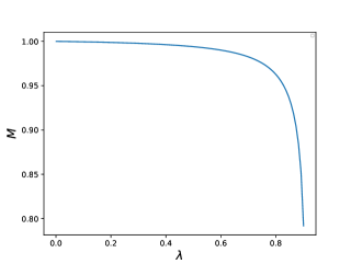
Figure 1: $M$ function for $\sigma=1$ and reverse aspect ratio $\epsilon=0.1$

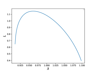
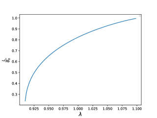
Figure 2: $L$ and $L/\theta_{b}$ functions for reverse aspect ratio $\epsilon=0.1$

This work was supported by the Italian Ministry for Foreign Affairs and International Cooperation Project under Grant No. CN23GR02.

Appendix A

In this appendix, the detailed expressions for Maxwellian distribution function are given. The Maxwellian distribution is

$$F_{0s}=\frac{n_{s}}{\left(2\pi{\cal E}_{ts}\right)^{3/2}}e^{-\frac{{\cal E}}{{\cal E}_{ts}}},$$ (A1)

where ${\cal E}_{ts}=T_{s}/m_{s}$. Then we have

$$D_{1} =\left(1+\frac{1}{\tau}\right)-\frac{n_{i}}{\sqrt{2}\pi N_{i}}\int_{0}^{1-\epsilon}\frac{K\left(\kappa^{-1}\right)}{\kappa\sqrt{\epsilon\lambda}}\left(1-\frac{\omega_{*ni}}{\omega}\right)d\lambda$$

$$-\frac{\sqrt{2}n_{e}}{\pi\tau N_{i}}\left(1-\frac{\omega_{*ne}}{\omega}+\frac{3}{2}\frac{\omega_{*Te}}{\omega}\right)\int_{1-\epsilon}^{1+\epsilon}\frac{K\left(\kappa\right)}{\sqrt{\epsilon\lambda}}\left[Z_{4}\left(\sqrt{\frac{\omega}{\bar{\omega}_{De}}}\right)-\frac{\omega}{\bar{\omega}_{De}}Z_{2}\left(\sqrt{\frac{\omega}{\bar{\omega}_{De}}}\right)\right]\sqrt{\frac{\bar{\omega}_{De}}{\omega}}d\lambda$$

$$+\frac{\sqrt{2}n_{e}}{\pi\tau N_{i}}\frac{\omega_{*Te}}{\omega}\int_{1-\epsilon}^{1+\epsilon}\frac{K\left(\kappa\right)}{\sqrt{\epsilon\lambda}}\left[Z_{6}\left(\sqrt{\frac{\omega}{\bar{\omega}_{De}}}\right)-\frac{\omega}{\bar{\omega}_{De}}Z_{4}\left(\sqrt{\frac{\omega}{\bar{\omega}_{De}}}\right)\right]\sqrt{\frac{\bar{\omega}_{De}}{\omega}}d\lambda$$

$$-\frac{\sqrt{2}n_{i}}{\pi N_{i}}\left(1-\frac{\omega_{*ni}}{\omega}+\frac{3}{2}\frac{\omega_{*Ti}}{\omega}\right)\int_{1-\epsilon}^{1+\epsilon}\frac{K\left(\kappa\right)}{\sqrt{\epsilon\lambda}}\sqrt{\frac{\bar{\omega}_{Di}}{\omega}}\left[Z_{4}\left(\sqrt{\frac{\omega}{\bar{\omega}_{Di}}}\right)-\frac{\omega}{\bar{\omega}_{Di}}Z_{2}\left(\sqrt{\frac{\omega}{\bar{\omega}_{Di}}}\right)\right]d\lambda$$

$$+\frac{\sqrt{2}n_{i}}{\pi N_{i}}\frac{\omega_{*Ti}}{\omega}\int_{1-\epsilon}^{1+\epsilon}\frac{K\left(\kappa\right)}{\sqrt{\epsilon\lambda}}\sqrt{\frac{\bar{\omega}_{Di}}{\omega}}\left[Z_{6}\left(\sqrt{\frac{\omega}{\bar{\omega}_{Di}}}\right)-\frac{\omega}{\bar{\omega}_{De}}Z_{4}\left(\sqrt{\frac{\omega}{\bar{\omega}_{Di}}}\right)\right]d\lambda,$$ (A2)

$$D_{2} =\left(1+\frac{1}{\tau}\right)+\frac{\sqrt{2}n_{e}}{\pi\tau N_{i}}\left(1-\frac{\omega_{*ne}}{\omega}+\frac{3}{2}\frac{\omega_{*Te}}{\omega}\right)\int_{1-\epsilon}^{1+\epsilon}\frac{K\left(\kappa\right)}{\sqrt{\epsilon\lambda}}\sqrt{\frac{\omega}{\bar{\omega}_{De}}}Z_{2}\left(\sqrt{\frac{\omega}{\bar{\omega}_{De}}}\right)d\lambda$$

$$-\frac{\sqrt{2}n_{e}}{\pi\tau N_{i}}\frac{\omega_{*Te}}{\omega}\int_{1-\epsilon}^{1+\epsilon}\frac{K\left(\kappa\right)}{\sqrt{\epsilon\lambda}}\sqrt{\frac{\omega}{\bar{\omega}_{De}}}Z_{4}\left(\sqrt{\frac{\omega}{\bar{\omega}_{De}}}\right)d\lambda$$

$$+\frac{\sqrt{2}n_{i}}{\pi N_{i}}\left(1-\frac{\omega_{*ni}}{\omega}+\frac{3\omega_{*Ti}}{2\omega}\right)\int_{1-\epsilon}^{1+\epsilon}\frac{K\left(\kappa\right)}{\sqrt{\epsilon\lambda}}\sqrt{\frac{\omega}{\bar{\omega}_{Di}}}Z_{2}\left(\sqrt{\frac{\omega}{\bar{\omega}_{Di}}}\right)d\lambda$$

$$-\frac{\sqrt{2}n_{i}}{\pi N_{i}}\frac{\omega_{*Ti}}{\omega}\int_{1-\epsilon}^{1+\epsilon}\frac{K\left(\kappa\right)}{\sqrt{\epsilon\lambda}}\sqrt{\frac{\omega}{\bar{\omega}_{Di}}}Z_{4}\left(\sqrt{\frac{\omega}{\bar{\omega}_{Di}}}\right)d\lambda$$

$$-\frac{n_{i}}{\sqrt{2}\pi N_{i}}\int_{0}^{1-\epsilon}\frac{K\left(\kappa^{-1}\right)}{\kappa\sqrt{\epsilon\lambda}}\left(1-\frac{\omega_{*ni}}{\omega}\right)d\lambda,$$ (A3)

$$N_{i}=\frac{n_{i}}{\sqrt{2}\pi}\left(\int_{0}^{1-\epsilon}\frac{K\left(\kappa^{-1}\right)}{\kappa\sqrt{\epsilon\lambda}}d\lambda+\int_{1-\epsilon}^{1+\epsilon}\frac{K\left(\kappa\right)}{\sqrt{\epsilon\lambda}}d\lambda\right),$$ (A4)

where

$$Z_{n}\left(x\right)=\frac{2x}{\sqrt{\pi}}\int_{0}^{\infty}\frac{t^{n}e^{-t^{2}}}{t^{2}-x^{2}}dt.$$ (A5)

For even $n$, $Z_{n}\left(x\right)=xZ_{n-1}\left(x\right)$. For odd $n$, $Z_{n}\left(x\right)=xZ_{n-1}\left(x\right)+\Gamma\left(n/2\right)/\sqrt{\pi}$. $Z_{0}\left(x\right)$ is the so-called plasma dispersion function. And $\Gamma\left(x\right)$ is the Gamma function. Here the functions in $\kappa$ are treated as functions in $\lambda$ for simplicity of notation. Then we have

$$D_{3} =\frac{\sqrt{2}n_{i}}{\pi N_{i}}\left(1-\frac{\omega_{*ni}}{\omega}+\frac{3}{2}\frac{\omega_{*Ti}}{\omega}\right)\int_{1-\epsilon}^{1+\epsilon}\frac{\omega}{\bar{\omega}_{Di}}\frac{L^{2}K\left(\kappa\right)}{\sqrt{\epsilon\lambda}}\left(2-\lambda\right)\left(\frac{\omega}{\bar{\omega}_{Di}}G_{4}-G_{6}\right)d\lambda$$

$$-\frac{\sqrt{2}n_{i}}{\pi N_{i}}\frac{\omega_{*Ti}}{\omega}\int_{1-\epsilon}^{1+\epsilon}\frac{\omega}{\bar{\omega}_{Di}}\frac{L^{2}K\left(\kappa\right)}{\sqrt{\epsilon\lambda}}\left(2-\lambda\right)\left(\frac{\omega}{\bar{\omega}_{Di}}G_{6}-G_{8}\right)d\lambda$$

$$-\frac{\sqrt{2}n_{i}}{\pi N_{i}}\left(1-\frac{\omega_{*ni}}{\omega}+\frac{3}{2}\frac{\omega_{*Ti}}{\omega}\right)\int_{0}^{1-\epsilon}\frac{M^{2}K\left(\kappa^{-1}\right)}{\kappa\sqrt{\epsilon\lambda}}\left(2-\lambda\right)\frac{\omega}{\omega_{Bi}}Z_{4}\left(\frac{\omega}{\omega_{Bi}}\right)d\lambda$$

$$+\frac{\sqrt{2}n_{i}}{\pi N_{i}}\frac{\omega_{*Ti}}{\omega}\int_{0}^{1-\epsilon}\frac{M^{2}K\left(\kappa^{-1}\right)}{\kappa\sqrt{\epsilon\lambda}}\left(2-\lambda\right)\frac{\omega}{\omega_{Bi}}Z_{6}\left(\frac{\omega}{\omega_{Bi}}\right)d\lambda,$$ (A6)

$$D_{4} =\left(1+\frac{1}{\tau}\right)-\frac{\sqrt{2}n_{i}}{\pi N_{i}}\left(1-\frac{\omega_{*ni}}{\omega}+\frac{3}{2}\frac{\omega_{*Ti}}{\omega}\right)\int_{1-\epsilon}^{1+\epsilon}\frac{\omega}{\bar{\omega}_{Di}}\frac{L^{2}K\left(\kappa\right)}{\sqrt{\epsilon\lambda}}\left(\frac{\omega}{\bar{\omega}_{Di}}G_{2}-G_{4}\right)d\lambda$$

$$+\frac{\sqrt{2}n_{i}}{\pi N_{i}}\frac{\omega_{*Ti}}{\omega}\int_{1-\epsilon}^{1+\epsilon}\frac{\omega}{\bar{\omega}_{Di}}\frac{L^{2}K\left(\kappa\right)}{\sqrt{\epsilon\lambda}}\left(\frac{\omega}{\bar{\omega}_{Di}}G_{4}-G_{6}\right)d\lambda$$

$$+\frac{\sqrt{2}n_{i}}{\pi N_{i}}\left(1-\frac{\omega_{*ni}}{\omega}+\frac{3}{2}\frac{\omega_{*Ti}}{\omega}\right)\int_{0}^{1-\epsilon}\frac{M^{2}K\left(\kappa^{-1}\right)}{\kappa\sqrt{\epsilon\lambda}}\frac{\omega}{\omega_{Bi}}Z_{2}\left(\frac{\omega}{\omega_{Bi}}\right)d\lambda$$

$$-\frac{\sqrt{2}n_{i}}{\pi N_{i}}\frac{\omega_{*Ti}}{\omega}\int_{0}^{1-\epsilon}\frac{M^{2}K\left(\kappa^{-1}\right)}{\kappa\sqrt{\epsilon\lambda}}\left(2-\lambda\right)\frac{\omega}{\omega_{Bi}}Z_{4}\left(\frac{\omega}{\omega_{Bi}}\right)d\lambda,$$ (A7)

where

$$G_{n} =\frac{1}{\sqrt{\pi}}\int_{0}^{\infty}\frac{2t^{n}e^{-t^{2}}}{\left(\omega/\bar{\omega}_{Di}-t^{2}\right)^{2}-\omega_{Bi}^{2}t^{2}/\bar{\omega}_{Di}^{2}}dt$$

$$=\frac{1}{\Omega_{1}^{2}-\Omega_{2}^{2}}\left[\frac{1}{\Omega_{1}}Z_{n}\left(\Omega_{1}\right)-\frac{1}{\Omega_{2}}Z_{n}\left(\Omega_{2}\right)\right],$$ (A8)

$$\Omega_{1}=\frac{\frac{\omega_{Bi}}{\bar{\omega}_{Di}}+\sqrt{\frac{4\omega}{\bar{\omega}_{Di}}+\frac{\omega_{Bi}^{2}}{\bar{\omega}_{Di}^{2}}}}{2},$$ (A9)

and

$$\Omega_{2}=\frac{-\frac{\omega_{Bi}}{\bar{\omega}_{Di}}+\sqrt{\frac{4\omega}{\bar{\omega}_{Di}}+\frac{\omega_{Bi}^{2}}{\bar{\omega}_{Di}^{2}}}}{2}.$$ (A10)

Thus, $N_{0}=D_{1}/D_{2}$ and $N_{s}=D_{3}/D_{4}$ are given. For the inertia terms, we have

$$\Lambda_{fl}^{2}=\frac{\omega\left(\omega-\omega_{*Pi}\right)}{2\pi\omega_{A}^{2}}N_{0}\left(\int_{0}^{1-\epsilon}\lambda^{1/2}\frac{3\sqrt{2}K\left(\kappa^{-1}\right)}{2\kappa\sqrt{\epsilon}}d\lambda+\int_{1-\epsilon}^{1+\epsilon}\frac{3\sqrt{2}\lambda^{1/2}K\left(\kappa\right)}{2\sqrt{\epsilon}}d\lambda\right),$$ (A11)

$$\Lambda_{circ}^{2} =\frac{\sqrt{2}\omega_{ti}^{2}}{4\pi\omega_{A}^{2}}q^{2}\omega\left(1-\frac{\omega_{*ni}}{\omega}+\frac{3}{2}\frac{\omega_{*Ti}}{\omega}\right)\int_{0}^{1-\epsilon}\frac{K\left(\kappa^{-1}\right)M^{2}}{\omega_{Bi}\kappa\sqrt{\epsilon\lambda}}\left(2-\lambda\right)\left[N_{s}Z_{4}\left(\frac{\omega}{\omega_{Bi}}\right)+\left(2-\lambda\right)Z_{6}\left(\frac{\omega}{\omega_{Bi}}\right)\right]d\lambda$$

$$-\frac{\sqrt{2}\omega_{ti}^{2}}{4\pi\omega_{A}^{2}}q^{2}\omega_{*Ti}\int_{0}^{1-\epsilon}\frac{K\left(\kappa^{-1}\right)M^{2}}{\omega_{Bi}\kappa\sqrt{\epsilon\lambda}}\left(2-\lambda\right)\left[N_{s}Z_{6}\left(\frac{\omega}{\omega_{Bi}}\right)+\left(2-\lambda\right)Z_{8}\left(\frac{\omega}{\omega_{Bi}}\right)\right]d\lambda,$$ (A12)

and

$$\Lambda_{tr}^{2} =-\frac{\sqrt{2}\omega_{ti}^{2}}{4\pi\omega_{A}^{2}}q^{2}\left(1-\frac{\omega_{*ni}}{\omega}+\frac{3}{2}\frac{\omega_{*Ti}}{\omega}\right)\int_{1-\epsilon}^{1+\epsilon}\frac{\omega^{2}}{\bar{\omega}_{Di}^{2}}\frac{K\left(\kappa\right)L^{2}}{\sqrt{\epsilon\lambda}}\left(2-\lambda\right)\left[N_{s}G_{4}+G_{6}\left(2-\lambda\right)\right]d\lambda$$

$$+\frac{\sqrt{2}\omega_{ti}^{2}}{4\pi\omega_{A}^{2}}q^{2}\frac{\omega_{*Ti}}{\omega}\int_{1-\epsilon}^{1+\epsilon}\frac{K\left(\kappa\right)\left(2-\lambda\right)L^{2}}{\sqrt{\epsilon\lambda}}\frac{\omega^{2}}{\bar{\omega}_{Di}^{2}}\left[\left(2-\lambda\right)G_{8}+N_{s}G_{6}\right]d\lambda$$

$$+\frac{\sqrt{2}\omega_{ti}^{2}}{4\pi\omega_{A}^{2}}q^{2}\left(1-\frac{\omega_{*ni}}{\omega}+\frac{3}{2}\frac{\omega_{*Ti}}{\omega}\right)\int_{1-\epsilon}^{1+\epsilon}\frac{K\left(\kappa\right)\left(2-\lambda\right)L^{2}}{\sqrt{\epsilon\lambda}}\frac{\omega}{\bar{\omega}_{Di}}\left[\left(2-\lambda\right)G_{8}+N_{s}G_{6}\right]d\lambda$$

$$-\frac{\sqrt{2}\omega_{ti}^{2}}{4\pi\omega_{A}^{2}}q^{2}\frac{\omega_{*Ti}}{\omega}\int_{1-\epsilon}^{1+\epsilon}\frac{K\left(\kappa\right)\left(2-\lambda\right)L^{2}}{\sqrt{\epsilon\lambda}}\frac{\omega}{\bar{\omega}_{Di}}\left[G_{10}\left(2-\lambda\right)+N_{s}G_{8}\right]d\lambda,$$ (A13)

where $\omega_{A}=v_{A}/qR_{0}$ and $v_{A}=B_{0}/\sqrt{4\pi n_{i}m_{i}}$.

References

- [1] Chen L and Zonca F 2016 Reviews of Modern Physics 88 015008
- [2] Zonca F and Chen L 2014 Physics of Plasmas 21 072120
- [3] Zonca F and Chen L 2014 Physics of Plasmas 21 072121
- [4] Brizard A and Hahm T 2007 Reviews of Modern Physics 79 421–468
- [5] Frieman E A and Chen L 1982 Physics of Fluids 25 502
- [6] Chen L and Zonca F 2017 Physics of Plasmas 24 072511
- [7] Chavdarovski I and Zonca F 2009 Plasma Phys Contr F 51 115001
- [8] Bierwage A and Lauber P 2017 Nuclear Fusion 57 116063
- [9] Lauber P and Lu Z 2018 Journal of Physics: Conference Series 1125 012015
- [10] Choi G J, Liu P, Wei X S, Nicolau J H, Dong G, Zhang W L, Lin Z, Heidbrink W W and Hahm T S 2021 Nuclear Fusion 61 066007
- [11] Falessi M V, Carlevaro N, Fusco V, Vlad G and Zonca F 2019 Physics of Plasmas 26 082502
- [12] Gao Z, Itoh K, Sanuki H and Dong J Q 2008 Physics of Plasmas 15 072511
- [13] Biancalani A, Bottino A, Ehrlacher C, Grandgirard V, Merlo G, Novikau I, Qiu Z, Sonnendrücker E, Garbet X, Görler T, Leerink S, Palermo F and Zarzoso D 2017 Physics of Plasmas 24 062512
- [14] Zonca F and Chen L 1996 Physics of Plasmas 3 323–343
- [15] Zonca F, Chen L, Dong J Q and Santoro R A 1999 Physics of Plasmas 6 1917
- [16] Chavdarovski I and Zonca F 2014 Physics of Plasmas 21 052506
- [17] Heidbrink W W, Zeeland M A V, Austin M E, Crocker N A, Du X D, McKee G R and Spong D A 2021 Nuclear Fusion 61 066031
- [18] Gorelenkov N N, Pinches S D and Toi K 2014 Nuclear Fusion 54 125001 ISSN 0029-5515
- [19] Ma R, Heidbrink W W, Chen L, Zonca F and Qiu Z 2023 Physics of Plasmas 30 042105
- [20] Zonca F, Chen L, Briguglio S, Fogaccia G, Vlad G and Wang X 2015 New Journal of Physics 17 013052
- [21] Zonca F and Chen L 2006 Plasma physics and controlled fusion 48 537
- [22] Hinton F L and Hazeltine R D 1976 Reviews of Modern Physics 48 239–308
- [23] White R B and Chance M S 1984 Physics of Fluids 27 2455
- [24] Falessi M V, Chen L, Qiu Z and Zonca F 2023 Nonlinear equilibria and transport processes in burning plasmas (Preprint arXiv:2306.08642)