A Multi-Modal Approach Based on Large Vision Model for Close-Range Underwater Target Localization

Abstract

Underwater target localization uses real-time sensory measurements to estimate the position of underwater objects of interest, providing critical feedback information for underwater robots in tasks such as obstacle avoidance, scientific exploration, and environmental monitoring. While acoustic sensing is the most acknowledged and commonly used method in underwater robots and possibly the only effective approach for long-range underwater target localization, such a sensing modality generally suffers from low resolution, high cost and high energy consumption, thus leading to a mediocre performance when applied to close-range underwater target localization. On the other hand, optical sensing has attracted increasing attention in the underwater robotics community for its advantages of high resolution and low cost, holding a great potential particularly in close-range underwater target localization. However, most existing studies in underwater optical sensing are restricted to specific types of targets due to the limited training data available. In addition, these studies typically focus on the design of estimation algorithms and ignore the influence of illumination conditions on the sensing performance, thus hindering wider applications in the real world. To address the aforementioned issues, this paper proposes a novel target localization method that assimilates both optical and acoustic sensory measurements to estimate the 3D positions of close-range underwater targets. A test platform with controllable illumination conditions is designed and developed to experimentally investigate the proposed multi-modal sensing approach. A large vision model is applied to process the optical imaging measurements, eliminating the requirement for training data acquisition, thus significantly expanding the scope of potential applications. Extensive experiments are conducted, the results of which validate the effectiveness of the proposed underwater target localization method.

I Introduction

In recent years, a variety of underwater robots have been designed and developed by researchers and engineers worldwide [1], giving birth to a revolutionary paradigm of marine robotics. As a result of technological advancements, the applications of underwater robots grow rapidly covering missions and tasks across the scientific, industrial and military domains [2]. Particularly, close-range marine tasks such as marine life monitoring [3], shipwreck surveying [4], sea mining exploration [5], searching and rescuing [6] become achievable. To successfully accomplish these tasks, accurate target perception, particularly target localization, is the essential cornerstone.

To date, many underwater sensing methods have been designed to solve the close-range target localization problem [7], [8]. Among these methods, acoustic sensing, optical sensing and pressure sensing are the three mainstream types of sensory modalities [9]. Acoustic sensing with sonars is the most acknowledged and commonly-used approach in underwater robots and possibly the only feasible approach for long-range sensing tasks. Meanwhile, drawbacks such as insufficient resolution, high cost and high energy-consumption often lead to a mediocre estimation performance particularly in the close-range target localization task [10]. On the other hand, within a close distance, pressure sensing with artificial lateral lines excels in perceiving dynamic flows but typically suffers an inaccurate estimate and a degraded performance when dealing with (quasi-)static targets [11]. To resolve the close-range underwater target sensing problem, optical sensing has grasped a growing attention in the science and engineering communities due to its appealing features of high resolution and low cost. Although inappropriate for long-range underwater sensing due to the rapid light attenuation and light refraction [12], optical sensors are perfectly fit for close-range underwater tasks [13].

With the advancement of artificial intelligence, convolutional neural networks (CNNs), as a powerful tool in deep learning, have been applied to underwater sensory measurements for target sensing [14], [15]. For example, Islam et al. [16] designed a CNN tailored for diver tracking with camera images by modifying the building blocks of the state-of-the-art object detection CNN models and validated the designed model in both lab tanks and open-water environments. Li et al. [17] fine-tuned a general target detection algorithm running CNNs — the You Only Look Once (YOLO) model and successfully applied it to underwater optical images to detect marine life such as echini, starfish, and scallops. Sapienza et al. [18] proposed a pipeline leveraging the YOLO model and the augmented autoencoder (AAE) to compute 6-D pose estimates of targets from 2-D images and tested the method with objects including boxes, cups, and jugs in different underwater scenarios. Furthermore, researchers have investigated and designed a number of target localization methods for close-range underwater targets with dynamic motions [19], [20]. Wolek et al. [21] designed and tested a multi-target tracker to actively track nearby surface vessels using a passive sonar. Langis et al. [22] proposed a multi-diver tracking method that used camera images to detect human divers and estimate their dynamic motion states.

While the design of target localization using a single sensing modality, e.g., acoustic or optical sensing, suffices in estimating the motion states of underwater targets, employing multiple sensory modalities usually leads to higher estimation performances, which attracts a rapidly growing interest within the research community. For example, Remmas et al. [23] designed a data fusion scheme using a monocular camera, distributed hydrophones and pressure sensors and achieved accurate tracking of human divers. Xu et al. [24] presented an estimation method that fused measurement data from a forward-looking sonar, a monocular camera and an ultrasonic proximate sensor for underwater multi-target positioning. Jiang et al. [25] proposed a dual-sensor fusion modality integrating pressure sensors and flow velocity sensors to locate a near-field dipole source.

Whereas various underwater target localization approaches both in single and multiple modalities have been designed and tested, there still remain several challenging problems unresolved. First, most of the existing literature focuses on the network architecture design of deep learning models without considering the influence of the illumination condition on the target localization performance. With extremely low illumination, optical sensing is most likely unable to provide sufficiently accurate target estimates. Second, most of the methods are limited to a specific type of target. For the mainstream object detection models, large amount of labeled data are required to guarantee the accuracy of the target detection [26]. However, we don’t have the luxury of large-scale datasets of underwater targets, thus significantly impeding the wide application of the existing deep learning-based approaches.

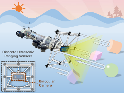
Figure 1: The schematic of the proposed multi-modal close-range target localization framework for underwater robots. When an underwater target appears within the sensor measurement range, multiple optical and acoustic sensors equipped onboard the underwater robot collaboratively estimate the motion states of the target of interest.

To address the issues mentioned above, this paper proposes a multi-modal sensing framework (illustrated in Fig. 1) that fuses real-time acoustic and optical sensory measurements utilizing a large vision model to achieve a general sensing capability of close-range underwater target localization. To validate the proposed approach, a test platform is designed and constructed with controllable lighting conditions. The test platform consists of a binocular camera taking the advantage of its high-precision and low-cost attributes [27] along with a number of distributed single-beam ultrasonic ranging sensors. We employ a large vision model — the Segment Anything Model (SAM) [28] to segment features from underwater images, which adopts the Transformer architecture [29]. Trained on the exhaustive SA-1B dataset with over 1 billion masks on 11 million images, SAM is a milestone model in vision history with the ability to segment any object in an image with proper prompt through user interaction [30]. The emergence of the large vision models sheds light on a new way to solve the underwater target localization problem. This paper investigates the feasibility and evaluates the performance of applying the SAM to the close-range underwater target localization with zero-shot transfer. Extensive experiments are conducted and experimental results are presented to confirm the multi-modal sensory design and the robustness of the proposed estimation algorithm with respect to illumination conditions.

The contributions of the paper are twofold. First, this paper proposes a novel multi-modal sensing method that incorporates a large vision model (SAM) to assimilate acoustic and optical sensory measurements for close-range underwater target localization. Owing to the superior generalization capability of the large vision model, the proposed method is expected to achieve an enhanced robust sensing performance with respect to various underwater targets with no training data required. Second, differing from most of the existing studies, this paper takes the illumination variance into consideration and conducts extensive experiments to quantitatively investigate and evaluate the influence of illumination conditions on the performance of the designed target localization algorithm.

II Test Platform

This paper designs and constructs a test platform to investigate the close-range target localization problem which consists of a sensing module, a target module, and a test pool. The sensing module, shown in Fig. 2(a), is comprised of a 3D-printed square-shaped support frame, a binocular camera located at the center of the frame, and eight acoustic ranging sensors located at the four corners and the four midpoints of the edges. We adopt binocular camera from ROVMAKER, supporting several resolutions, with 2560*960 as the highest resolution. The acoustic ranging sensors are the ultrasonic L04 modules by DYP Sensor. The target module consists of an acrylic frame that holds sphere-shaped and cube-shaped targets of different sizes and colors as shown in Fig. 2(b). The test pool measures 1.5m long, 1m wide and 0.7m deep. Two tunable LED tubes are attached onto the wall above the pool to control the illumination condition of the testing underwater environment. A HOBO MX2202 light intensity sensor is selected and mounted over against the LED tubes, to measure/record the experimental illumination condition. The sensing module moves along a sliding guide (Fig. 2(c)) installed above the pool with accurate position control implemented using a stepper motor of model 86BYG with 4.1N·m holding torque from Mecheltron and a Raspberry Pi 4B. The eight ultrasonic ranging sensors point directly to the center of their corresponding grids of the acrylic frame that hold potential targets. A Jetson Xavier is adopted to collect the sensor measurements and process the data for target localization and tracking in real time.

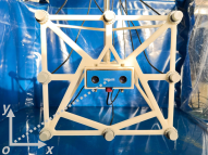
(a) The designed sensing module.

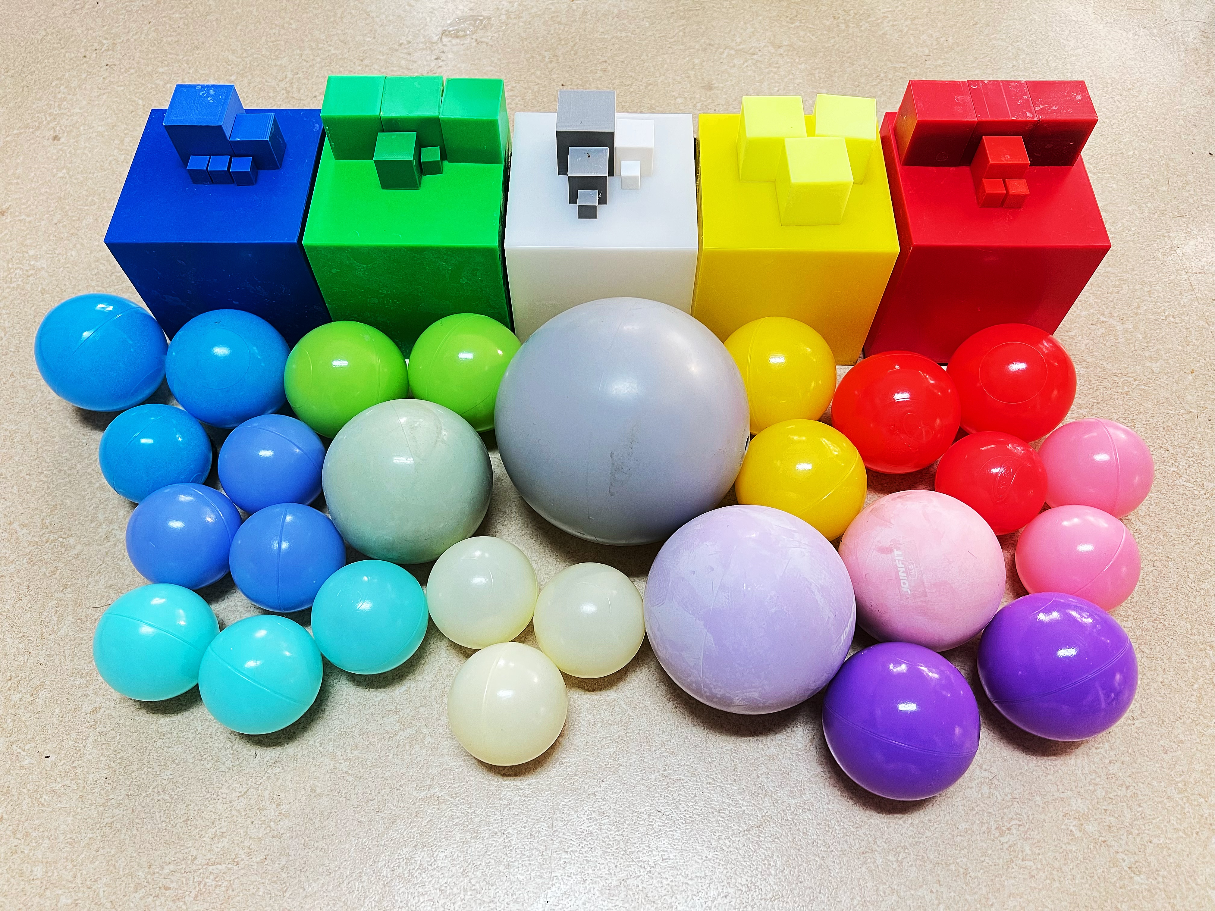
(b) The selected targets.

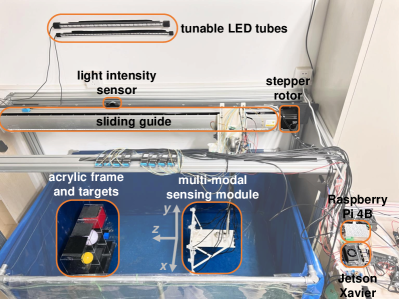
(c) Layout of the test platform.

Figure 2: Illustration of the test platform and the relevant components.

III Camera Model Preliminaries

This section reviews the camera models and defines the variable notations used in this paper. The camera models include the pinhole model, the distortion model and the binocular model specifically.

III-A Pinhole Camera Model

Following the conventions in camera modeling [31], this paper adopts three coordinate reference frames to describe the target and related image transformations including the world, the camera, and the pixel reference frames. The 3D coordinates of a point P in the world reference frame represented by $\textbf{{P}}_{\text{w}}=[X_{\text{w}},Y_{\text{w}},Z_{\text{w}}]^{\text{T}}$ are projected to the 3D coordinates in the camera reference frame represented by $\textbf{{P}}_{\text{c}}=[X_{\text{c}},Y_{\text{c}},Z_{\text{c}}]^{\text{T}}$ following a linear transformation, i.e.,

$$\textbf{{P}}_{\text{c}}=\textbf{{R}}_{\text{c}}\textbf{{P}}_{\text{w}}+\textbf{{t}}_{\text{c}},$$ (1)

where $\textbf{{R}}_{\text{c}}$ is the 3-by-3 rotation matrix and $\textbf{{t}}_{\text{c}}$ is the 3-by-1 translation vector. $\textbf{{R}}_{\text{c}}$ and $\textbf{{t}}_{\text{c}}$ are the camera extrinsics.

Projecting $\textbf{{P}}_{\text{c}}$ to the 2D pixel reference frame, the corresponding coordinates $\textbf{{P}}_{\text{p}}=[u,v,1]^{\text{T}}$ follow a homogeneous form, i.e.,

$$\textbf{{P}}_{\text{p}}=\frac{1}{Z_{\text{c}}}\begin{bmatrix}\textit{f}_{\textit{x}}&\textit{0}&\textit{c}_{\textit{x}}\\ \textit{0}&\textit{f}_{\textit{y}}&\textit{c}_{\textit{y}}\\ \textit{0}&\textit{0}&\textit{1}\end{bmatrix}\textbf{{P}}_{\text{c}}=\frac{1}{Z_{\text{c}}}\textbf{{KP}}_{\text{c}},$$ (2)

where K is the camera intrinsic matrix, $[c_{x},c_{y}]^{\text{T}}$ represents the position of the principal point, which is the intersection of the line perpendicular to the imaging plane passing through the pinhole with the imaging plane. $[f_{x},f_{y}]^{\text{T}}$ represents the focal lengths with respect to the $x$ and $y$ directions, respectively. Ignoring the manufacturing flaws and calibration errors of the camera, $f_{x}$ is equal to $f_{y}$ and referred to as $f$ in the following sections.

III-B Distortion Model

Lenses are introduced into the camera model to mitigate performance conflicts between crispness and brightness [32]. Image distortion occurs with the presence of a lens which alters the light propagation path. There are two types of distortion, namely radial distortion and tangential distortion. Radial distortion is caused by the shape of the lens while tangential distortion is induced by the misalignment between the lens and the image plane.

Denote the coordinates of a point P on the target in the camera coordinate frame by $[X_{\text{c}},Y_{\text{c}},Z_{\text{c}}]^{\text{T}}$. Obtain the normalized the coordinates $[x_{\text{n}},y_{\text{n}}]^{\text{T}}$ by

$$\begin{bmatrix}x_{\text{n}}\\ y_{\text{n}}\end{bmatrix}=\begin{bmatrix}X_{\text{c}}/Z_{\text{c}}\\ Y_{\text{c}}/Z_{\text{c}}\end{bmatrix}.$$ (3)

Calculate the distance $r$ between P and the origin, i.e.,

$$r=\sqrt{x_{\text{n}}^{2}+y_{\text{n}}^{2}}.$$ (4)

The radial distortion $[x_{\text{dr}},y_{\text{dr}}]^{\text{T}}$ is calculated as

$$\begin{bmatrix}x_{\text{dr}}\\ y_{\text{dr}}\end{bmatrix}=(1+k_{1}r^{2}+k_{2}r^{4}+k_{3}r^{6})\begin{bmatrix}x_{\text{n}}\\ y_{\text{n}}\end{bmatrix},$$ (5)

where $\textbf{{D}}_{\text{r}}=[k_{1},k_{2},k_{3}]$ represents the radial distortion parameters.

The tangential distortion $[x_{\text{dt}},y_{\text{dt}}]^{\text{T}}$ is described by

$$\begin{bmatrix}x_{\text{dt}}\\ y_{\text{dt}}\end{bmatrix}=\begin{bmatrix}x_{\text{n}}\\ y_{\text{n}}\end{bmatrix}+2x_{\text{n}}y_{\text{n}}\begin{bmatrix}p_{1}\\ p_{2}\end{bmatrix}+r^{2}\begin{bmatrix}p_{2}\\ p_{1}\end{bmatrix}+2\begin{bmatrix}p_{2}x_{\text{n}}^{2}\\ p_{1}y_{\text{n}}^{2}\end{bmatrix},$$ (6)

where $\textbf{{D}}_{\text{t}}=[p_{1},p_{2}]$ represents the tangential distortion parameters. Define distortion parameter vector $\textbf{{D}}=[\textbf{{D}}_{\text{r}},\textbf{{D}}_{\text{t}}]$.

The total distortion $[x_{\text{d}},y_{\text{d}}]^{\text{T}}$ is then defined as

$$\begin{bmatrix}x_{\text{d}}\\ y_{\text{d}}\end{bmatrix}=\begin{bmatrix}x_{\text{dr}}\\ y_{\text{dr}}\end{bmatrix}+\begin{bmatrix}x_{\text{dt}}\\ y_{\text{dt}}\end{bmatrix}-\begin{bmatrix}x_{\text{n}}\\ y_{\text{n}}\end{bmatrix}.$$ (7)

Projecting the point to the pixel coordinate frame through intrinsic parameters, we obtain

$$\begin{bmatrix}u\\ v\end{bmatrix}=\begin{bmatrix}f_{x}x_{\text{d}}\\ f_{y}y_{\text{d}}\end{bmatrix}+\begin{bmatrix}c_{x}\\ c_{y}\end{bmatrix},$$ (8)

where $[u,v]^{\text{T}}$ represents the 2-D coordinates of point P in the pixel reference frame.

III-C Binocular Camera Model

Binocular stereo vision mimics the distance perception of human eyes. Stereo images are acquired by two (or more) cameras set at different locations. A matching algorithm finds the corresponding points in those stereo images. The target distance is then calculated using the triangulation method. A binocular camera consists of two monocular cameras, namely the left view camera and the right view camera. Each monocular camera has its own intrinsic matrix $\textbf{{K}}_{\text{L}}$, $\textbf{{K}}_{\text{R}}$ and distortion parameters $\textbf{{D}}_{\text{L}}=[\textbf{{D}}_{\text{L,r}},\textbf{{D}}_{\text{L,t}}]$, $\textbf{{D}}_{\text{R}}=[\textbf{{D}}_{\text{R,r}},\textbf{{D}}_{\text{R,t}}]$. The extrinsic parameters, the rotation matrix $\textbf{{R}}_{\text{b}}$ and the translation vector $\textbf{{t}}_{\text{b}}$, are necessary to describe the relative attitude and position between two monocular cameras of the binocular camera.

Figure 3 illustrates the principle of the stereo vision in our experiment. The green cubes represent the targets to be localized. The blue cuboid represents the binocular camera and the two parallelograms represent the imaging planes of the left and right cameras. $\textbf{{O}}_{\text{L}}$ and $\textbf{{O}}_{\text{R}}$ are the left and right aperture centers, respectively; $f$ is the focal length; and $b$ is the baseline of the stereo system. For a point P on target, $\textbf{{P}}_{\text{L}}$ and $\textbf{{P}}_{\text{R}}$ are the coordinates of P in the left and right images, respectively. $u_{\text{L}}$ and $-u_{\text{R}}$ are the horizontal coordinates of $\textbf{{P}}_{\text{L}}$ and $\textbf{{P}}_{\text{R}}$. Considering that the triangle $\bigtriangleup\textbf{{P}}\textbf{{P}}_{\text{L}}\textbf{{P}}_{\text{R}}$ is similar to the triangle $\bigtriangleup\textbf{{P}}\textbf{{O}}_{\text{L}}\textbf{{O}}_{\text{R}}$, the target distance $Z$ is calculated using triangulation as

$$Z=\frac{fb}{u_{\text{L}}-u_{\text{R}}}=\frac{fb}{d_{u}},$$ (9)

where $d_{u}$ is the binocular disparity.

Theoretically speaking, $\textbf{{P}}_{\text{L}}$ and $\textbf{{P}}_{\text{R}}$ share the same vertical coordinate after rectification. However, due to calibration and localization error, a difference in the vertical coordinates exists. Define vertical disparity $d_{\text{v}}$ as the difference in the vertical coordinates, and epipolar tolerance $\varepsilon$ as the maximum difference in pixels allowed along the vertical direction. The epipolar matching condition (EMC) is satisfied if

$$d_{v}=|v_{\text{L}}-v_{\text{R}}|<\epsilon,$$ (10)

where $v_{\text{L}}$ and $v_{\text{R}}$ are the vertical coordinates of $\textbf{{P}}_{\text{L}}$ and $\textbf{{P}}_{\text{R}}$.

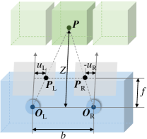
Figure 3: Illustration of the principle of stereo vision used in the experiment.

IV Underwater Target Localization Design

This section presents the multi-modal approach for close-range underwater target localization. Section IV-A designs a target detection algorithm that uses a large vision model and ranging sensor prompts to obtain the target distance from stereo images. Section IV-B presents the filtering design for the ranging task and the motion state estimation task of dynamic targets.

The proposed multi-modal target localization algorithm is illustrated in Algorithm 1. The algorithm takes the video stream from the binocular camera and the ranging data stream from the acoustic sensors as inputs to calculate the positions and velocities of the targets of interest in real time. To avoid ambiguity, we use frame to refer to the stereo image with both views at a given time step and image to refer to either the left or the right view image whose width is half width of a frame.

Algorithm 1 Multi-Modal Target Localization.

0:  Real-time binocular video frame $I_{\text{b}}$

0:  Real-time ranging measurement data $I_{\text{r}}$

0:  3-D position and velocity of the target(s), denoted as $\textbf{{P}}=[p_{x},p_{y},p_{z}]^{\text{T}}$ and $\textbf{{V}}=[v_{x},v_{y},v_{z}]^{\text{T}}$ respectively, or indication of “no target”

1:  Initialize hyper-parameters including intrinsic matrices $\textbf{{K}}_{\text{L}}/\textbf{{K}}_{\text{R}}$, distortion parameters $\textbf{{D}}_{\text{L}}/\textbf{{D}}_{\text{R}}$, extrinsic parameters $\textbf{{R}}_{\text{b}}$ and $\textbf{{t}}_{\text{b}}$, number of measurements for extrapolation $n_{\text{f}}$, segmentation confidence threshold $c_{\text{s}}^{\text{th}}$, epipolar tolerance $\varepsilon$, ranging data effective threshold $r_{\text{max}}^{\text{th}}$ and $r_{\text{min}}^{\text{th}}$, fusion weight $\alpha$, process noise covariance matrix Q and measurement noise covariance matrix R.

2:  while new frame do

3:     Calibrate current ranging data.

4:     if ranging data $>r_{\text{max}}^{\text{th}}$ or $<r_{\text{min}}^{\text{th}}$ then

5:        Ranging data is labeled ineffective. Extrapolate from previous $n_{\text{f}}$ ranging data measurements.

6:     end if

7:     Rectify current frame using $\textbf{{K}}_{\text{L}}$, $\textbf{{K}}_{\text{R}}$, $\textbf{{D}}_{\text{L}}$, $\textbf{{D}}_{\text{R}}$, $\textbf{{R}}_{\text{b}}$ and $\textbf{{t}}_{\text{b}}$.

8:     Perform target segmentation with SAM and calculate minimum bounding box per Section IV-A.

9:     if any segmentation mask confidence $<c_{\text{s}}^{\text{th}}$ then

10:        Segmentation of current target in image fails, extrapolate from previous $n_{\text{f}}$ bounding boxes.

11:     end if

12:     Calculate vertical disparities of key point pairs of each target $\{d_{v}^{i},i=1,...,5\}$ per Section IV-A.

13:     if $\exists i,\text{s.t. }d_{v}^{i}>\varepsilon$ then

14:        Segmentation of current target in frame fails, extrapolate from previous $n_{\text{f}}$ bounding boxes.

15:     end if

16:     if only target ranging is desired then

17:        Implement the weighted averaging filter per Section IV-B1

18:     else if 3-D target position and velocity information is desired then

19:        Implement EKF per Section IV-B2

20:     end if

21:  end while

IV-A Target Detection With Large Vision Model and Ranging Sensor Prompts

The proposed sensing module consists of a binocular camera and several ultrasonic ranging sensors. The binocular camera is selected as the primary sensor for close-range target localization while ultrasonic ranging sensors provide rough inference of the target location. Comprehensively considering the sensing accuracy performance and the practical limitations in the computational resource and the transmission bandwidth, the number of the ultrasonic ranging sensors is selected to achieve the balance therebetween, specifically eight sensors in this paper as an example.

This paper adopts a large vision model — SAM in the target detection process aiming to achieve a high generalization capability with no training data required. SAM requires a prompt of either a point or a bounding box, provided by the ranging sensors.

The transmission and reception angles of the ultrasonic ranging sensors are typically restricted to a certain acute angle, which is correlated to the transducer structure and the transmission frequency. As long as the target is within the reception field, the following procedure applies.

Align the world coordinate frame with the camera coordinate frame. Set an upper limit $r_{\text{max}}^{\text{th}}$ and a lower limit $r_{\text{min}}^{\text{th}}$ for the ranging data. Monitor all the ranging sensor outputs in real time. When one or more of the range measurements are within the distance threshold, project the 3-D target position onto the 2-D pixel coordinate frame. Define the coordinates of a detected point P on the target in the camera coordinate frame as $[X_{\text{c}},Y_{\text{c}},Z_{\text{c}}]^{\text{T}}$. $X_{\text{c}}$ and $Y_{\text{c}}$ are typically constant according to the structural design of the sensing module and $Z_{\text{c}}$ is acquired by the ranging sensor(s). The 2-D coordinates $[u,v]^{\text{T}}$ of point P in the pixel coordinate frame are obtained per Section III-B. The 2-D point(s) is then used as prompt input(s) for the SAM model to begin the segmentation process.

With images and proper prompt(s), SAM is applied to obtain segmentation masks, after which minimum bounding box is achieved for each target. Define the center point pair and four corner point pairs as the five key point pairs set in the left and right images for each target. Obtain coordinates of the five key point pairs of the target, denoted as $\{\left[\textbf{{P}}_{\text{L}}^{\text{1}}=(u_{\text{L}}^{\text{1}},v_{\text{L}}^{\text{1}}),\textbf{{P}}_{\text{R}}^{\text{1}}=(u_{\text{R}}^{\text{1}},v_{\text{R}}^{\text{1}})\right],$ $...,\left[\textbf{{P}}_{\text{L}}^{\text{5}}=(u_{\text{L}}^{\text{5}},v_{\text{L}}^{\text{5}}),\textbf{{P}}_{\text{R}}^{\text{5}}=(u_{\text{R}}^{\text{5}},v_{\text{R}}^{\text{5}})\right]\}$. Calculate vertical disparities of key point pairs, denoted as $\{d_{v}^{\text{1}},...,d_{v}^{\text{5}}\}$. Check whether or not the EMC is satisfied for each pair per Eq. (10). If EMC is satisfied for all five key point pairs, the segmentation masks in paired images are matched successfully, indicating the same target. Distance $Z_{\text{i}}$ where $i=1,...,5$, of each point is calculated by Eq. (9). Averaged over the five distances, the estimate of the distance of the target is obtained. Otherwise, if any of the five vertical disparities fails EMC, the segmentation masks of the target in current frame are considered ineffective.

IV-B Multi-modal Target Localization

With pre-processed sensory data, both optical and acoustic sensing modalities are used in underwater target localization. Two types of filtering are designed to assimilate the multi-modal sensor measurements including the weighted averaging filter and the extended Kalman filter (EKF) for target ranging and target motion state estimation, respectively. The filters are selected considering a balance between localization performance and the real-time computational cost.

IV-B1 Target ranging with the weighted averaging filter

A light intensity sensor is used to monitor the light intensity for further investigation of segmentation and localization success rate under different light intensities. A factor $\alpha\in[0,1]$ that balances between the measurement from optical sensor and from acoustic sensors is designed

$$Z_{\text{f}}=\alpha*Z_{\text{b}}+(1-\alpha)*Z_{\text{r}},$$ (11)

where $Z_{\text{b}},Z_{\text{r}}$ and $Z_{\text{f}}$ represent the distance estimates by the binocular camera alone, the ultrasonic ranging sensors alone, and the multi-modal sensor fusion.

Define the ground truth distance and the estimated distance as $Z_{\text{gt}}$ and $Z_{\text{m}}$ respectively. The estimation percentage error is then defined as $e=\left(\left|Z_{\text{m}}-Z_{\text{gt}}\right|/Z_{\text{gt}}\right)\times 100\%$. Parameter $\alpha$ is designed and calculated following an intuitive formula utilizing the averaged estimation percentage error of both sensor modalities. The average distance estimation percentage error of the ranging sensor $\bar{e_{\text{r}}}$ is obtained from the datasheet. Under a certain illumination intensity, to estimate the distance estimation percentage error of the binocular camera denoted as $\bar{e_{\text{b}}}$, we take $M$ frames with $N$ targets each frame and calculate $\bar{e_{\text{b}}}$ by

$$\bar{e_{\text{b}}}=\frac{1}{M\times N}{\textstyle\sum_{1}^{M}}{\textstyle\sum_{1}^{N}}e_{\text{b}}^{m,n},$$ (12)

where $e_{\text{b}}^{m,n}$ represents the distance estimation percentage error of the $n^{\text{th}}$ target in the $m^{\text{th}}$ frame.

The weight $\alpha$ is then calculated as

$$\alpha=\frac{\bar{e_{\text{r}}}}{\bar{e_{\text{b}}}+{\bar{e_{\text{r}}}}}.$$ (13)

Furthermore, if target segmentation in frame $t$ fails, the current distance value from binocular camera $Z_{\text{b}}^{t}$ is then extrapolated from the previous distance estimates $Z_{\text{b}}^{t-1},...,Z_{\text{b}}^{t-n}$. The same extrapolation method is applicable to ultrasonic ranging data as well.

IV-B2 Target motion state estimation using EKF

We first establish the estimation model including the dynamic system state equation and the observation equation. Consider a dynamic target traveling through water whose position and velocity are both to be estimated. We define the estimation state vector as follows

$$\textbf{{x}}=\begin{bmatrix}p_{x}&p_{y}&p_{z}&v_{x}&v_{y}&v_{z}\end{bmatrix}^{\text{T}},$$ (14)

where the first three elements are the position states and the last three elements are the velocity states in the $x,y,z$ directions, respectively.

The state equation is given in a compact form as

$$\textbf{{x}}_{\textit{k}}=\textbf{{A}}\textbf{{x}}_{\textit{k}\text{-1}}+\textbf{{B}}\textbf{{u}}_{\textit{k}_{\text{-1}}}+\textbf{{w}}_{\textit{k}}.$$ (15)

Here, w is the process noise and the distribution $p(\textbf{{w}})\sim N(\textbf{{{0}}},\textbf{{{Q}}})$ where Q is the process noise covariance matrix. Considering the focus of this paper is to investigate the the feasibility and evaluate the performance of the multi-modal close-range underwater target localization using a large vision model, we select and implement a representative motion to study in which the target is controlled to travel at a constant speed. The system matrix A and the input matrix B are then given by $\textbf{{A}}=\begin{bmatrix}\textbf{{I}}_{\text{3}}&t\textbf{{I}}_{\text{3}}\\ \textbf{{0}}_{\text{3}}&\textbf{{I}}_{\text{3}}\end{bmatrix}$ , $\textbf{{B}}=\textbf{{0}}_{\text{6*1}}.$

Define the measurement vector as follows

$$\textbf{{z}}=\begin{bmatrix}u&v&d_{u}&d_{r}\end{bmatrix}^{\text{T}},$$ (16)

where $[u,v]^{\text{T}}$ is the 2-D coordinate in the image coordinate system, $d_{u}$ is the disparity value calculated from the binocular camera and $d_{r}$ is the distance value from the ranging sensor.

The measurement equation is in the form of

$$\textbf{{z}}_{\textit{k}}=\textbf{{h}}(\textbf{{x}}_{\textit{k}})+\textbf{{v}}_{\textit{k}},$$ (17)

where nonlinear function vector h is described as

$$\textbf{{h}}(\textbf{{x}}_{\textit{k}})=\begin{bmatrix}\dfrac{f_{u}p_{x}}{p_{z}}+c_{u},\dfrac{f_{v}p_{y}}{p_{z}}+c_{v},\dfrac{bf_{u}}{p_{z}},p_{z}\end{bmatrix}^{\text{T}},$$ (18)

v is the measurement noise and the distribution $p(\textbf{{v}})\sim N(\textbf{{{0}}},\textbf{{{R}}})$, where R is the measurement noise covariance matrix.

The Jacobian matrix H is the partial derivatives of h with respect to x, i.e.,

$$\textbf{{H}}=\begin{bmatrix}\dfrac{f_{u}}{p_{z}}&0&-\dfrac{f_{u}p_{x}}{p_{z}^{2}}&0&0&0\\ 0&\dfrac{f_{v}}{p_{z}}&-\dfrac{f_{v}p_{y}}{p_{z}^{2}}&0&0&0\\ 0&0&-\dfrac{bf_{u}}{p_{z}^{2}}&0&0&0\\ 0&0&1&0&0&0\end{bmatrix},$$ (19)

The process noise w in our experiment mainly comes from the vibration of the guiding system travelling through water and is modeled as follows. We consider the vibration in the system results in a non-zero acceleration of the sensing module which follows a Gaussian process with zero mean and a constant variation. The variances of the position and the velocity as well as the covariance between the position and the velocity are then calculated accordingly. Assuming that the external forces are independent along the $x,y,z$ axes, and within a small time interval $\Delta t$ the accelerations $a_{x},a_{y},a_{z}$ in the $x,y,z$ axes are all constant, the resulting velocity and position $v_{x},v_{y},v_{z}$ and $p_{x},p_{y},p_{z}$ follow Gaussian distributions. The variances of $v_{x}$ and $p_{x}$ are calculated as follows and $v_{y},v_{z}$ and $p_{y},p_{z}$ compute similarly.

$$\sigma(v_{x})=\sigma(a_{x}\Delta t)=(\Delta t)^{2}\sigma(a_{x}),$$ (20)

$$\sigma(p_{x})=\sigma(\frac{1}{2}a_{x}(\Delta t)^{2})=\frac{1}{4}(\Delta t)^{4}\sigma(a_{x}).$$ (21)

The covariance between the position and the velocity along the same axis is then calculated as

$$\sigma(p_{x},v_{x})=\sqrt{\sigma(p_{x})}\sqrt{\sigma(v_{x})}=\frac{1}{2}(\Delta t)^{3}\sigma(a_{x}),$$ (22)

The process noise covariance matrix Q is given by

$$\textbf{{Q}}=\begin{bmatrix}\dfrac{1}{4}(\Delta t)^{4}\textbf{{Q}}_{\text{b}}&\dfrac{1}{2}(\Delta t)^{3}\textbf{{Q}}_{\text{b}}\\ \dfrac{1}{2}(\Delta t)^{3}\textbf{{Q}}_{\text{b}}&(\Delta t)^{2}\textbf{{Q}}_{\text{b}}\end{bmatrix},$$ (23)

where $\textbf{{Q}}_{\text{b}}=\text{diag}(\sigma(a_{x}),\sigma(a_{y}),\sigma(a_{z}))$ is the 3-by-3 building block diagonal matrix.

V Experiments

This section presents the implementation setup of the physical experiments, the experimental results, and the corresponding analyses.

V-A Implementation Setup

The binocular camera was calibrated using a checkerboard with $9\times 12$ square grids of 2 cm by 2 cm dimension. The calibration was completed in water using the open source computer vision library — OpenCV. Intrinsic parameters and distortion parameters of the binocular camera are listed in Table I. The extrinsic parameters of the binocular system are listed in Table II. The transmission frequency of the ultrasonic ranging sensors is 1 MHz.

TABLE I: Intrinsic parameters

View	Intrinsic Parameters				Radial Distortion Parameters			Tangential Distortion Parameters
	$\textbf{{f}}_{\textbf{{x}}}$	$\textbf{{f}}_{\textbf{{y}}}$	$\textbf{{c}}_{\textbf{{x}}}$	$\textbf{{c}}_{\textbf{{y}}}$	$\textbf{{k}}_{\textbf{{1}}}$	$\textbf{{k}}_{\textbf{{2}}}$	$\textbf{{k}}_{\textbf{{3}}}$	$\textbf{{p}}_{\textbf{{4}}}$	$\textbf{{p}}_{\textbf{{5}}}$
Left	$1.241\times 10^{3}$	$1.187\times 10^{3}$	$6.61\times 10^{2}$	$5.06\times 10^{2}$	$2.92\times 10^{-1}$	$9.98\times 10^{-1}$	$-1.74$	$3.30\times 10^{-3}$	$-2.64\times 10^{-3}$
Right	$1.242\times 10^{3}$	$1.184\times 10^{3}$	$6.93\times 10^{2}$	$5.25\times 10^{2}$	$2.92\times 10^{-1}$	$8.97\times 10^{-1}$	$-1.13$	$1.12\times 10^{-3}$	$-1.56\times 10^{-3}$

TABLE II: Extrinsic Parameters

Rotation	$\begin{bmatrix}9.99\times 10^{-1}&2.08\times 10^{-3}&-9.35\times 10^{-3}\\ -2.03\times 10^{-3}&9.99\times 10^{-1}&5.62\times 10^{-3}\\ 9.36\times 10^{-3}&-5.60\times 10^{-3}&9.99\times 10^{-1}\end{bmatrix}$
Translation	$\begin{bmatrix}-59.02&0.17&-0.43\end{bmatrix}$

As shown in Fig. 4, a total of five scenes with 35 targets were designed and used in the experiment. All the images were rectified with camera calibration parameters.

(a) Scene 1.

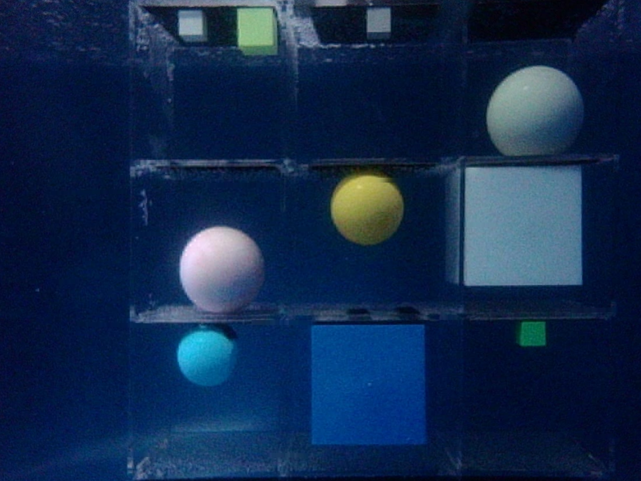
(b) Scene 2.

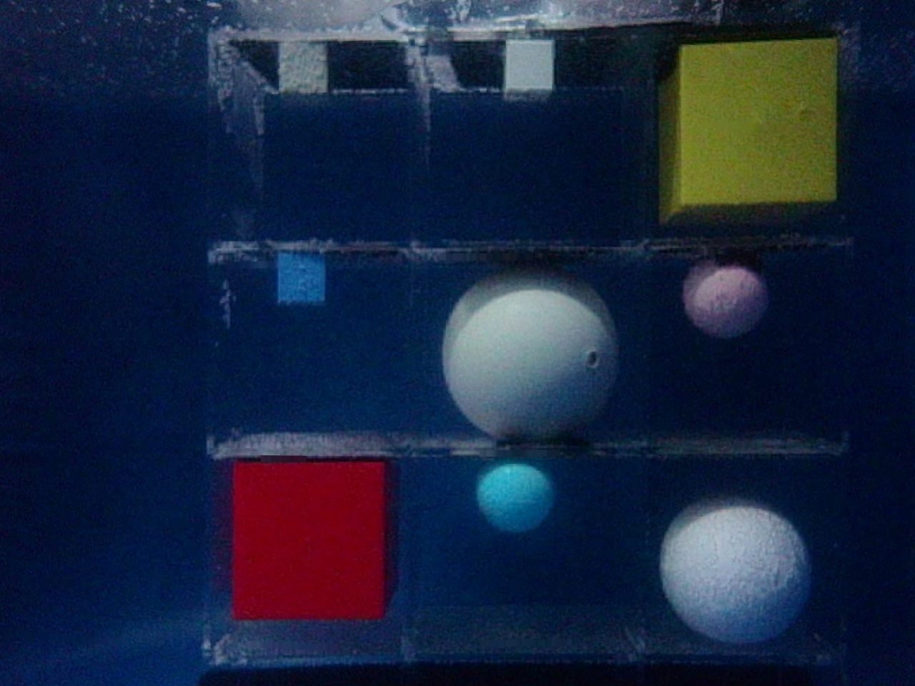
(c) Scene 3.

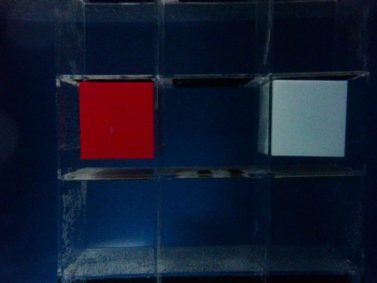
(d) Scene 4.

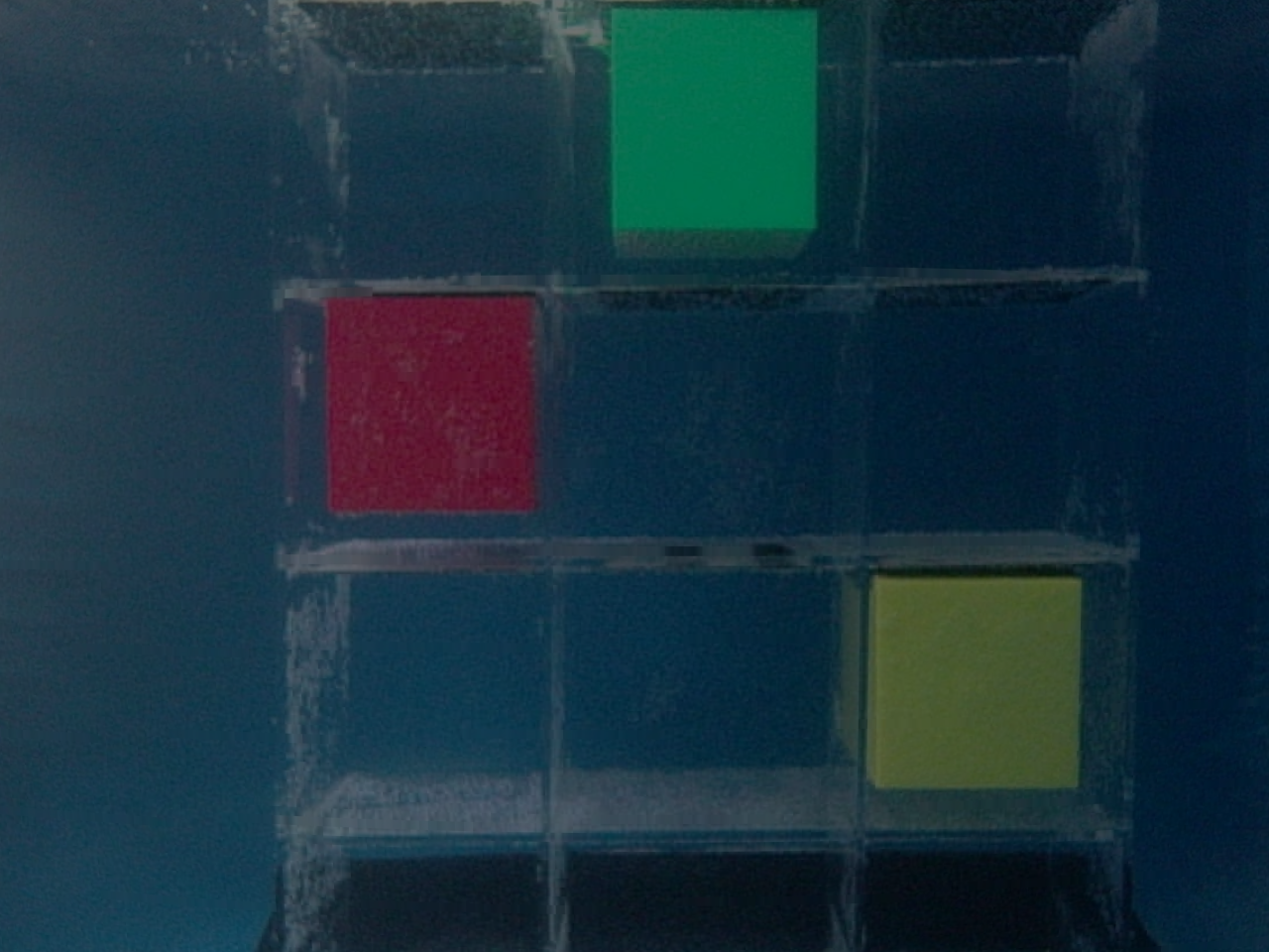
(e) Scene 5.

Figure 4: Layout of the five test scenes. Scene 1 includes 11 targets placed at a distance of 50 cm from the sensing module. Scene 2 includes 10 targets placed at a distance of 55 cm. Scene 3 includes 9 targets at a distance of 60 cm. Scenes 4 and 5 include 2 and 3 targets of dynamic motion, respectively. Scene 1 shows the paired left and right view images of the binocular camera while Scenes 2-5 show only the left view images.

The experiment mainly includes three tasks. In the first task, the targets are stationary. The segmentation capability of SAM and the influence of the light intensity on the ranging estimation performance are comprehensively studied with extensive experiments. In the second and third tasks, 1-D ranging and 3-D position & velocity estimation of dynamic targets are investigated. For dynamic targets, the sensing module moves along the sliding guide at a constant speed of either 1.25cm/s or 0.5cm/s. The weighted averaging and the EKF filters are used in tasks 2 and 3, respectively.

V-B Experimental Results

V-B1 Task 1

Scenes 1-3 with totally 30 static targets were used in the experiment. We leveraged the controllable LED tubes to adjust the environmental illumination and a light intensity sensor to quantify the lighting conditions (Fig. 2). Seven illumination conditions were created including 25 lux, 12 lux, 10 lux, 8 lux, 6 lux, 4 lux and 2 lux while 25 lux represents the normal daylight environment and others mimic different illumination levels in the underwater environment.

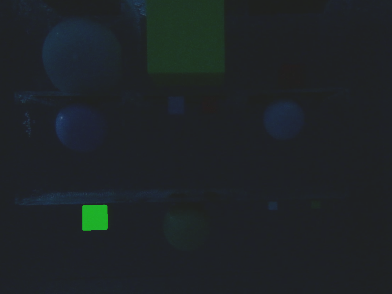
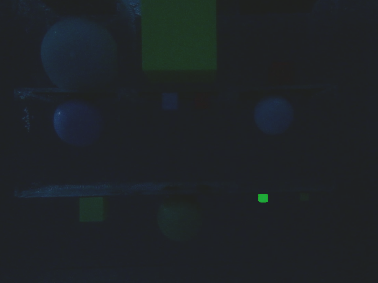
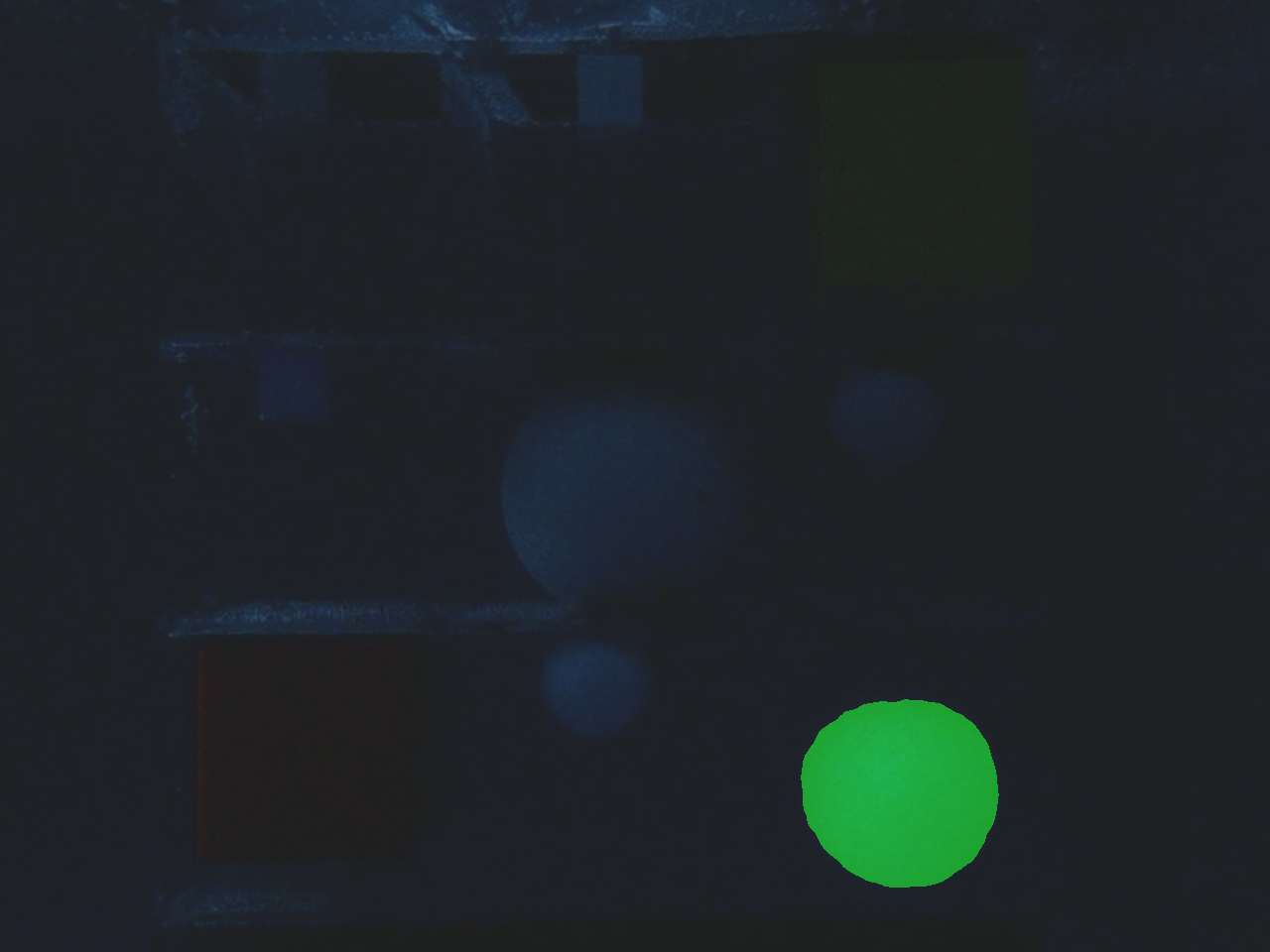
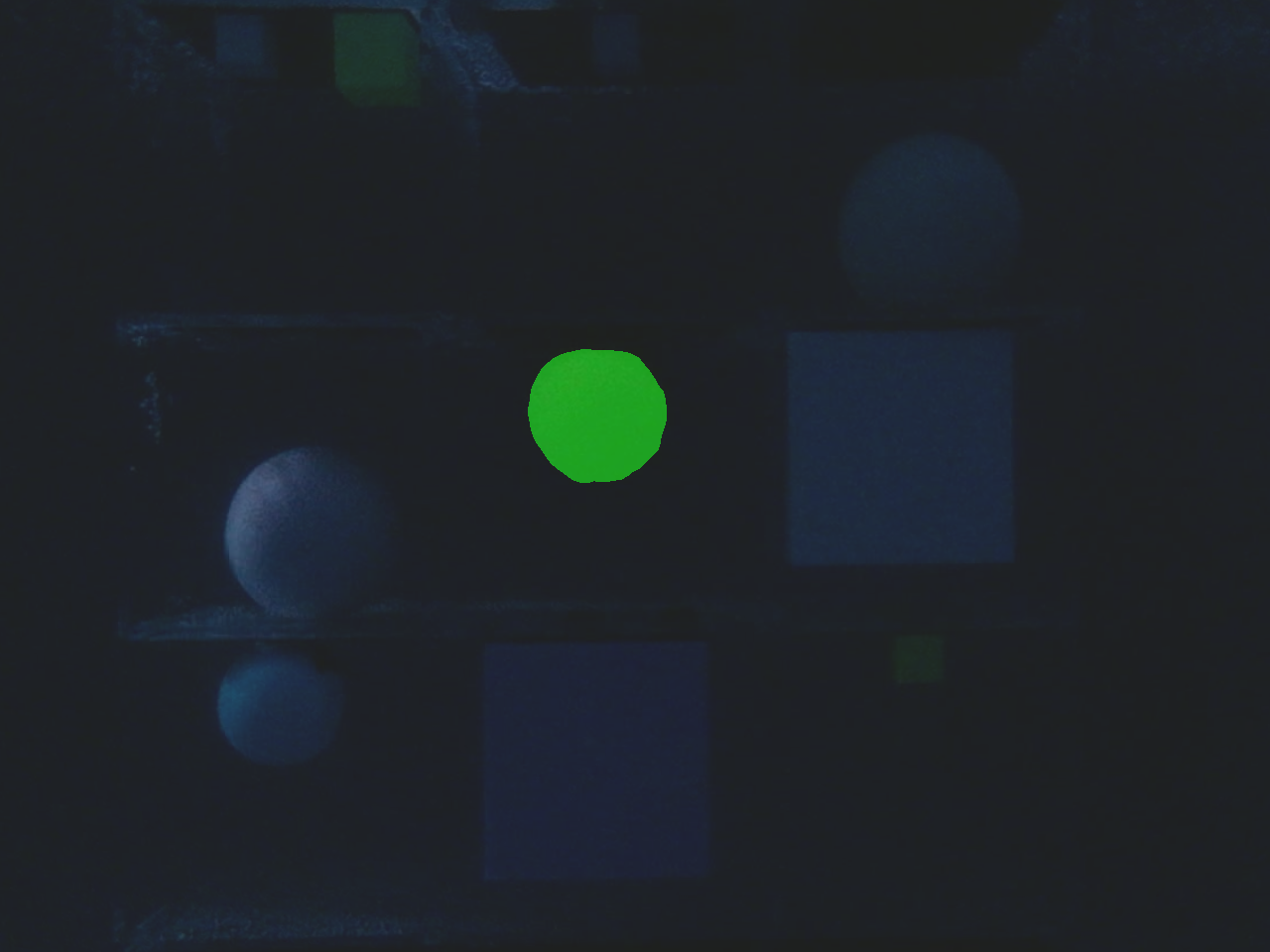
Figure 5: Illustration of the segmentation experimental results using the large vision model — SAM with the ranging sensor measurements as prompt inputs. The segmentation masks are superimposed on the original images. Three successfully segmented cube cases, three successfully segmented sphere cases and three segmentation failure cases are demonstrated.

Target segmentation with a large vision model. To quantitatively evaluate the performance of the SAM-based segmentation, we adopted the Intersection over Union (IoU) metric. When the IoU between the segmentation mask and the ground truth is lower than 60$\%$ for any single target, we consider the target segmentation as a failure. In addition, if the EMC (Eq. 10) is not satisfied which indicates a target matching failure in the left and right view images, the segmentation is considered as a failure . Otherwise, we have a successful segmentation. Examples of successful and failed segmentation are demonstrated in Fig. 5 with masks superimposed on the original images. Figure 6 shows the segmentation failure rate with respect to the illumination conditions. From the experimental results, we observe that when the illumination is greater than or equal to 8 lux, no failure exists. If the illumination intensity continues to decrease, the segmentation failure rate increases significantly with a roughly 2% failure rate at 6 lux, 12% at 4 lux, and over 70% at 2 lux.

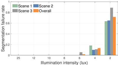
Figure 6: Experimental results of the statistical segmentation failure rate with respect to the illumination intensity in the three testing scenes.

Distance estimation by stereo vision. As the illumination decreases, not only the SAM-based segmentation success rate decreases but also its performance in terms of the segmentation accuracy, which results in an increased distance estimation error $\bar{e_{b}}$ (Eq. 12). Figures 7 and 8 present the experimental results of the segmentation IoU and the distance estimation percent error with respect to the illumination intensity, respectively. In all the three testing scenes, the averaged segmentation accuracy consistently decreases when the illumination intensity decreases. We observe that the IoU is over 90% at 25 lux and drops to around 75% at 2 lux (the calculation is based on successful target segmentation only). Similarly, the estimated distance using the stereo vision computation has a consistently increasing estimation percentage error ranging from 4% to 5.5% as the illumination intensity decreases from 25 lux to 2 lux. In addition, we also observe that the size and the shape of the targets influence the segmentation results as well. For example, larger targets generally lead to more accurate segmentation than their smaller counterparts, and cubes are segmented more accurately than spheres. Segmentation results are also susceptible to the illumination angle due to the existence of shadows, especially for spheres.

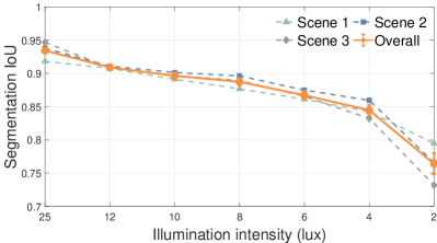
Figure 7: The experimental results of the segmentation IoU with respect to the illumination intensity. The lines of Scenes 1-3 plot the averaged IoU of all the targets in each scene. The error-bar of Overall plots the averaged value and the standard deviation of the IoU of all the targets in the three testing scenes.

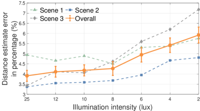
Figure 8: The experimental results of the distance estimation percentage error $\bar{e_{b}}$ with respect to the illumination intensity. $\bar{e_{b}}$ represents the averaged distance estimation percentage error over all the targets in one testing scene. The error-bar of Overall plots the averaged value and the standard deviation of $\bar{e_{b}}$ among all the three testing scenes.

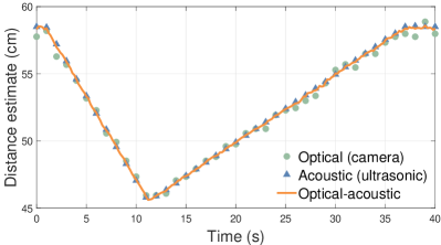
Figure 9: Trajectories of the multi-modal estimated distance between the sensing module and the dynamic target in the experiment. The ranging estimation using only the optical measurements (camera) and the acoustic measurements (ultrasonic) are provided as a comparison. The experimental results shows an enhanced estimation performance with a higher accuracy and a lower variance using both sensing modalities.

V-B2 Task 2

This experimental task estimates the time-varying distance between a moving target and the sensing module per Section IV-B1. A weighted averaging filter balances between the acoustic and optical sensor measurements with the design parameter $\alpha$ calculated based on the stereo camera ranging accuracy and the acoustic ranging sensor accuracy. The experiment adopted the 4 lux illumination condition where the large vision model SAM occasionally fails the image segmentation. We selected two large cubic targets (as shown in Fig. 4(d)) that typically lead to a higher segmentation success rate than other sized and/or shaped objects. Such an experimental setup is expected to alleviate overwhelming segmentation failures and help us to focus on the performance evaluation of the multi-modal ranging design for dynamic targets.

The distance estimation percentage error of the binocular camera under 4 lux illumination (Fig. 8) is $\bar{e_{\text{b}}}=5.42\%$ and that of the acoustic ranging sensor is $\bar{e_{\text{r}}}=1.75\%$. By Eq. (13), we calculate the weighting parameter $\alpha=0.24$. In this experiment, we selected two travelling speeds of the moving target, 1.25cm/s and 0.5cm/s when moving towards and farther away from the sensing module, respectively. Figure 9 shows the trajectory of the averaged ranging estimation error using the stereo vision, acoustic ranging, and both sensing modalities. From the experimental result, the averaged ranging estimation error over time using the binocular camera and the ultrasonic ranging sensors separately are 0.45% and 0.21%, respectively. The averaged ranging estimation error of the fused optical and acoustic measurements is 0.18%, thus providing a more accurate estimate than using either sensing modality alone.

TABLE III: The estimation errors in the target position and velocity states averaged over the entire motion process.

Scene	Estimation	$\boldsymbol{p_{x}}$ (m)	$\boldsymbol{p_{y}}$ (m)	$\boldsymbol{p_{z}}$ (m)	$\boldsymbol{v_{x}}$ (m/s)	$\boldsymbol{v_{y}}$ (m/s)	$\boldsymbol{v_{z}}$ (m/s)
Scene 4	Prior	$5.3\times 10^{-4}$	$3.1\times 10^{-4}$	$2.8\times 10^{-3}$	$9.3\times 10^{-4}$	$6.2\times 10^{-4}$	$1.5\times 10^{-3}$
	Posterior	$4.2\times 10^{-4}$	$2.3\times 10^{-4}$	$2.3\times 10^{-3}$	$8.3\times 10^{-4}$	$5.1\times 10^{-4}$	$1.1\times 10^{-3}$
Scene 5	Prior	$2.1\times 10^{-4}$	$1.3\times 10^{-4}$	$1.1\times 10^{-3}$	$3.2\times 10^{-4}$	$2.8\times 10^{-4}$	$7.1\times 10^{-4}$
	Posterior	$1.8\times 10^{-4}$	$1.0\times 10^{-4}$	$7.2\times 10^{-4}$	$2.8\times 10^{-4}$	$2.1\times 10^{-4}$	$6.6\times 10^{-4}$

V-B3 Task 3

This task assimilates optical and acoustic sensor measurements via EKF to estimate the 3-D motion states including the position and the velocity of a moving target of interest. The covariance matrix Q of the EKF is determined per Section IV-B2. We adopt Scenes 4 and 5 in Fig. 4 and use the sliding guide to move the targets along the $z$-axis as shown in Fig. 2. For the convenience of presentation and analysis, we subtract the $x$ and $y$ coordinates of the estimated target position by the actual constant coordinates and redefine the difference as $p_{x}$ and $p_{y}$. Consequently, in our experimental setup, the estimated target motion states along the $x$ and $y$ directions, i.e., $p_{x}$, $p_{y}$, $v_{x}$ and $v_{y}$ conform to normal distributions with a zero mean. In Scene 4, the acrylic frame that holds two cubic targets moves farther away from the sensing module at a speed of 0.5 cm/s for 20 seconds. In Scene 5, the acrylic frame holding three cubic targets moves towards the sensing module at a faster speed of 1.25 cm/s for 8 seconds. The averaged position estimates $\bar{p_{x}}$, $\bar{p_{y}}$, $\bar{p_{z}}$ and the averaged velocity estimates $\bar{v_{x}}$, $\bar{v_{y}}$, $\bar{v_{z}}$ over all the targets in each experimental setup are presented in Figs. 10 and 11 for Scenes 4 and 5, respectively. Furthermore, the estimation errors for each motion state in Scenes 4 and 5 are provided in Table III with both priors and posteriors of the EKF estimation. From the experimental results, we observe a consistent estimation error in both the position and velocity motion states in the magnitude of $10^{-3}$m or less along the $x$ and $y$ axes perpendicular to the direction of travel, and a slightly increased estimation error along the direction of travel. Averaged over all time instants, all the position and velocity state estimation errors are bounded by $2.8\times 10^{-3}$m and $1.5\times 10^{-3}$ m/s. In addition, by comparing the prior and posterior state estimates, we find that incorporating the multi-modal sensor measurements aligns with our design expectations and generally improves the estimation accuracy, reducing the averaged estimation error by 10% to 25%.

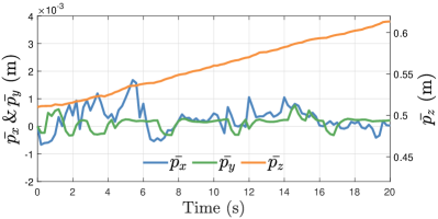
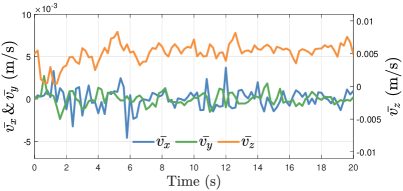
Figure 10: Trajectories of the position and velocity motion state estimates in the experiment in Scene 4 where the targets move father away from the sensing module at the speed of 0.5 cm/s.

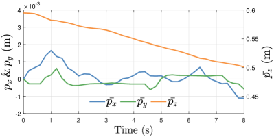
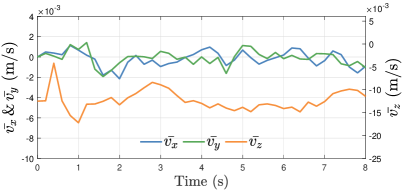
Figure 11: Trajectories of the position and velocity motion state estimates in the experiment in Scene 5 where the targets move towards the sensing module at the speed of 1.25 cm/s.

VI Conclusion

This paper proposed a multi-modal sensing framework to resolve the close-range underwater target localization problem with generalization capability. A sensing module consisting a stereo vision camera and eight acoustic ranging sensors was designed and developed along with a testing platform. A target localization algorithm was proposed which incorporated image segmentation through a large vision model (SAM) and multi-modal sensor fusion through weighted averaging and the EKF according to the sensing tasks. Extensive experiments were conducted, the results of which validated the effectiveness of the proposed multi-modal sensing framework in 1-D ranging and 3-D motion state estimation for both static and dynamic underwater targets. Furthermore, we experimentally investigated and quantitatively evaluated the influence of the illumination intensity on the target localization performance, aiming to provide important insights into the multi-modal sensing design in underwater environments.

For future work, we will explore the feasibility of replacing SAM with semantic and light-weight large vision models in image segmentation to improve real-time performance. In addition, we plan to install the multi-modal sensing module onto a lab-developed underwater robot and explore the application of the proposed estimation algorithm in the closed-loop motion control of underwater robots.

References

- [1] J. Zhou, Y. Si, and Y. Chen, “A review of subsea auv technology,” Journal of Marine Science and Engineering, vol. 11, no. 6, p. 1119, 2023.
- [2] R. B. Wynn, V. A. Huvenne, T. P. Le Bas, B. J. Murton, D. P. Connelly, B. J. Bett, H. A. Ruhl, K. J. Morris, J. Peakall, D. R. Parsons et al., “Autonomous underwater vehicles (auvs): Their past, present and future contributions to the advancement of marine geoscience,” Marine geology, vol. 352, pp. 451–468, 2014.
- [3] S. Raine, R. Marchant, B. Kusy, F. Maire, and T. Fischer, “Point label aware superpixels for multi-species segmentation of underwater imagery,” IEEE Robotics and Automation Letters, vol. 7, no. 3, pp. 8291–8298, 2022.
- [4] B. Bingham, B. Foley, H. Singh, R. Camilli, K. Delaporta, R. Eustice, A. Mallios, D. Mindell, C. Roman, and D. Sakellariou, “Robotic tools for deep water archaeology: Surveying an ancient shipwreck with an autonomous underwater vehicle,” Journal of Field Robotics, vol. 27, no. 6, pp. 702–717, 2010.
- [5] E. Simetti, R. Campos, D. D. Vito, J. Quintana, G. Antonelli, R. Garcia, and A. Turetta, “Sea mining exploration with an uvms: Experimental validation of the control and perception framework,” IEEE/ASME Transactions on Mechatronics, vol. 26, no. 3, pp. 1635–1645, 2021.
- [6] S. Venkatesan, “Auv for search & rescue at sea-an innovative approach,” in 2016 IEEE/OES Autonomous Underwater Vehicles (AUV). IEEE, 2016, pp. 1–9.
- [7] L. Zhufeng, L. Xiaofang, W. Na, and Z. Qingyang, “Present status and challenges of underwater acoustic target recognition technology: A review,” Frontiers in Physics, vol. 10, p. 1044890, 2022.
- [8] X. Yuan, L. Guo, C. Luo, X. Zhou, and C. Yu, “A survey of target detection and recognition methods in underwater turbid areas,” Applied Sciences, vol. 12, no. 10, p. 4898, 2022.
- [9] Y. Cong, C. Gu, T. Zhang, and Y. Gao, “Underwater robot sensing technology: A survey,” Fundamental Research, vol. 1, no. 3, pp. 337–345, 2021.
- [10] K. Sun, W. Cui, and C. Chen, “Review of underwater sensing technologies and applications,” Sensors, vol. 21, no. 23, p. 7849, 2021.
- [11] L. DeVries, F. D. Lagor, H. Lei, X. Tan, and D. A. Paley, “Distributed flow estimation and closed-loop control of an underwater vehicle with a multi-modal artificial lateral line,” Bioinspiration & biomimetics, vol. 10, no. 2, p. 025002, 2015.
- [12] D. Q. Huy, N. Sadjoli, A. B. Azam, B. Elhadidi, Y. Cai, and G. Seet, “Object perception in underwater environments: A survey on sensors and sensing methodologies,” Ocean Engineering, vol. 267, p. 113202, 2023.
- [13] F. Xu, H. Wang, J. Wang, K. W. S. Au, and W. Chen, “Underwater dynamic visual servoing for a soft robot arm with online distortion correction,” IEEE/ASME Transactions on Mechatronics, vol. 24, no. 3, pp. 979–989, 2019.
- [14] S. Xu, M. Zhang, W. Song, H. Mei, Q. He, and A. Liotta, “A systematic review and analysis of deep learning-based underwater object detection,” Neurocomputing, 2023.
- [15] B. Teng and H. Zhao, “Underwater target recognition methods based on the framework of deep learning: A survey,” International Journal of Advanced Robotic Systems, vol. 17, no. 6, p. 1729881420976307, 2020.
- [16] M. J. Islam, M. Fulton, and J. Sattar, “Toward a generic diver-following algorithm: Balancing robustness and efficiency in deep visual detection,” IEEE Robotics and Automation Letters, vol. 4, no. 1, pp. 113–120, 2019.
- [17] J. Li, L. Shi, and S. Guo, “Yolov7-based land and underwater target detection and recognition,” in 2023 IEEE International Conference on Mechatronics and Automation (ICMA), 2023, pp. 1437–1442.
- [18] D. Sapienza, E. Govi, S. Aldhaheri, M. Bertogna, E. Roura, . Pairet, M. Verucchi, and P. Ardón, “Model-based underwater 6d pose estimation from rgb,” IEEE Robotics and Automation Letters, vol. 8, no. 11, pp. 7535–7542, 2023.
- [19] M. Kumar and S. Mondal, “Recent developments on target tracking problems: A review,” Ocean Engineering, vol. 236, 2021.
- [20] G. Guo, X. Wang, and H. Xu, “Review on underwater target detection, recognition and tracking based on sonar image,” Control Decis, 2018.
- [21] A. Wolek, J. McMahon, B. R. Dzikowicz, and B. H. Houston, “Tracking multiple surface vessels with an autonomous underwater vehicle: Field results,” IEEE Journal of Oceanic Engineering, vol. 47, no. 1, pp. 32–45, 2020.
- [22] K. De Langis and J. Sattar, “Realtime multi-diver tracking and re-identification for underwater human-robot collaboration,” in 2020 IEEE International Conference on Robotics and Automation (ICRA). IEEE, 2020, pp. 11 140–11 146.
- [23] W. Remmas, A. Chemori, and M. Kruusmaa, “Diver tracking in open waters: A low‐cost approach based on visual and acoustic sensor fusion,” Journal of Field Robotics, vol. 38, no. 3, pp. 494–508, May 2021. [Online]. Available: https://onlinelibrary.wiley.com/doi/10.1002/rob.21999
- [24] G. H. Xu, L. Y. Wu, K. Yu, C. Yang, and L. Yang, “Multi-target detection of underwater vehicle based on multi-sensor data fusion,” in ISOPE International Ocean and Polar Engineering Conference. ISOPE, 2012, pp. ISOPE–I.
- [25] Y. Jiang, Z. Gong, Z. Yang, Z. Ma, C. Wang, Y. Wang, and D. Zhang, “Underwater source localization using an artificial lateral line system with pressure and flow velocity sensor fusion,” IEEE/ASME Transactions on Mechatronics, vol. 27, no. 1, pp. 245–255, 2022.
- [26] M. J. Islam, C. Edge, Y. Xiao, P. Luo, M. Mehtaz, C. Morse, S. S. Enan, and J. Sattar, “Semantic segmentation of underwater imagery: Dataset and benchmark,” in 2020 IEEE/RSJ International Conference on Intelligent Robots and Systems (IROS). IEEE, 2020, pp. 1769–1776.
- [27] G. Huo, Z. Wu, J. Li, and S. Li, “Underwater target detection and 3d reconstruction system based on binocular vision,” Sensors, vol. 18, no. 10, p. 3570, 2018.
- [28] A. Kirillov, E. Mintun, N. Ravi, H. Mao, C. Rolland, L. Gustafson, T. Xiao, S. Whitehead, A. C. Berg, W.-Y. Lo, P. Dollár, and R. Girshick, “Segment anything,” 2023.
- [29] A. Vaswani, N. Shazeer, N. Parmar, J. Uszkoreit, L. Jones, A. N. Gomez, L. Kaiser, and I. Polosukhin, “Attention is all you need,” 2017.
- [30] X. Zhao, W. Ding, Y. An, Y. Du, T. Yu, M. Li, M. Tang, and J. Wang, “Fast segment anything,” 2023.
- [31] R. Szeliski, Computer vision: algorithms and applications. Springer Nature, 2022.
- [32] T. A. Clarke and J. G. Fryer, “The development of camera calibration methods and models,” The Photogrammetric Record, vol. 16, no. 91, pp. 51–66, 1998.