Diverse molecular gas excitations in quasar host galaxies at $z\sim 6$

Abstract

We present observations using the NOrthern Extended Millimetre Array (NOEMA) of CO and $\rm H_{2}O$ emission lines, and the underlying dust continuum in two quasars at $z\sim 6$, i.e., P215$-$16 at $z=5.78$ and J1429+5447 at $z=6.18$. Notably, among all published CO SLEDs of quasars at $z\sim 6$, the two systems reveal the highest and the lowest CO level of excitation, respectively. Our radiative transfer modeling of the CO SLED of P215$-$16 suggests that the molecular gas heated by AGN could be a plausible origin for the high CO excitation. For J1429+5447, we obtain the first well-sampled CO SLED (from transitions from 2-1 to 10-9) of a radio-loud quasar at $z\gtrsim 6$. Analysis of the CO SLED suggests that a single photo-dissociation region (PDR) component could explain the CO excitation in the radio-loud quasar J1429+5447. This work highlights the utility of the CO SLED in uncovering the ISM properties in these young quasar-starburst systems at the highest redshift. The diversity of the CO SLEDs reveals the complexities in gas conditions and excitation mechanisms at their early evolutionary stage.

1 Introduction

Active star formation has been detected in the host galaxies of quasars from the local to the distant universe, revealing co-evolution of the supermassive black holes (SMBHs) and galaxies (e.g., Kormendy & Ho 2013; Wang et al. 2013, 2016; Willott et al. 2015; Venemans et al. 2016; Decarli et al. 2017; Pensabene et al. 2020). The cold ($\rm\sim 100\ K$) interstellar medium (ISM) in the quasar host galaxies fuels both the active galactic nucleus (AGN) and the nuclear star formation. Observations of the molecular and atomic lines at submillimeter/millimeter wavelengths provide rich information about the physical conditions and heating power of the cold ISM, which are the keys to understanding the evolution of the young quasar hosts (e.g., Wang et al. 2011, 2013, 2016; Decarli et al. 2017, 2018, 2023; Venemans et al. 2018; Shao et al. 2019, 2022; Li et al. 2020a, b; Meyer et al. 2022).

The CO molecule, as the second most abundant species of the molecular ISM, gives the brightest molecular line emission in the (sub)millimeter regime. The CO spectral line energy distributions (SLEDs), i.e., the CO line fluxes as a function of rotational transition quantum number $J$, are sensitive diagnostics of the physical properties of the molecular gas (e.g., temperature, density, and radiation field strength). The low-$J$ ($J\leq 3$) CO emission lines directly constrain the total molecular gas mass of galaxies (e.g., Walter et al. 2003; Riechers et al. 2006, 2011a; Wang et al. 2011; Shao et al. 2019; Ramos Almeida et al. 2022; Montoya Arroyave et al. 2023). Low-$J$ CO lines are found to be sublinearly correlated with far-infrared (FIR) luminosity (e.g., Riechers et al. 2006; Riechers 2011b; Kamenetzky et al. 2016). The mid-$J$ ($4\leq J\leq 8$) CO lines are reported to be linearly correlated with FIR luminosity (e.g., Greve et al. 2014; Lu et al. 2014; Liu et al. 2015; Kamenetzky et al. 2016), which is consistent with the gas heated by the far-ultraviolet (FUV; 6 eV $<h\nu<$ 13.6 eV) photons from young-massive stars (Carilli & Walter, 2013). The high-$J$ ($J\geq 9$) CO lines require high temperature and density to be excited, and processes such as X-ray ($\sim 1-100$ keV) heating from the AGN, mechanical heating from shocks, and cosmic-ray heating are frequently proposed to explain their excitation (e.g., Weiß et al. 2007; Spinoglio et al. 2012; Meijerink et al. 2013; Li et al. 2020a). Thus, the CO SLEDs also serve as probes for discriminating between different gas heating scenarios (Meijerink & Spaans 2005; Meijerink et al. 2007; Spaans 2008), e.g., the photo-dissociation region (PDR), where the gas is heated by the far-ultraviolet (FUV) photons from young massive stars and the AGN-heated X-ray dominated region (XDR).

Searching for direct evidence of the influence of the AGN activity on the ISM excitation is observationally challenging even in local/low-$z$ well-studied samples. Valentino et al. (2021) find that for a sample of normal $z\sim 1-1.7$ galaxies that host AGNs, marginal correlations have been found between the presence and strength of AGNs and the CO excitation on galaxy scales. On nuclear scales of 250 pc, Esposito et al. (2022) report weak correlations between the CO excitation and either the X-ray or FUV flux in a sample of 35 local active galaxies, which suggests that neither the AGN nor star formation has a dominant effect on the gas excitation in the centers of these galaxies. Studies of CO SLEDs of individual local AGN host galaxies suggest a mix of a PDR component that contributes to the low-to-mid $J$ CO fluxes and an XDR that dominates the high-$J$ CO emission (e.g., van der Werf et al. 2010; Spinoglio et al. 2012; Pozzi et al. 2017; Mingozzi et al. 2018). Other mechanisms, such as mechanical heating by shocks, dense PDRs, and cosmic-ray heating, are also reported to dominate the high-$J$ CO excitation in some local AGN hosts and starburst galaxies (e.g., van der Werf et al. 2010; Spinoglio et al. 2012; Pellegrini et al. 2013).

Luminous quasars at high-$z$ represent the most luminous AGNs across redshifts. They are reported to be responsible for their high CO excitation at high-$J$. The lensed quasar APM 08279 at $z=3.9$, is currently the highest excited CO SLED ever published across redshifts. Its CO emission is detected within the central $\sim 550$ pc scale (Riechers et al., 2009), and the high CO excitation is best explained by the X-ray heating from the AGN (Weiß et al. 2007; Bradford et al. 2011). Another example is the Cloverleaf quasar at $z=2.6$, for which the CO SLED is best fitted with a combination of a PDR and an XDR component (Uzgil et al., 2016).

Observations of quasars at $z\sim 6$ from optical to (sub-) millimeter wavelengths reveal that $\sim 1/3$ of them reside in extremely active environments with rapid SMBH accretion at rates of $\dot{M_{\rm BH}}$ $>10$ $\rm M_{\sun}\ yr^{-1}$ and intense star formation at rates up to a few $\sim$ 1000 $\rm M_{\sun}\ yr^{-1}$ in the host galaxy (e.g., Wang et al. 2008; Carilli & Walter 2013; De Rosa et al. 2014; Venemans et al. 2020). In such systems, both the star formation and the SMBH activity lead to the injection of vast amounts of energy into the ISM of the host galaxy, making its ISM an ideal target to study the early co-evolution between the SMBHs and their host galaxies. Well-sampled CO SLEDs (with at least four transitions detected) have been obtained for five quasars at $z\sim 6$ (Bertoldi et al. 2003; Walter et al. 2003; Riechers et al. 2009; Gallerani et al. 2014; Carniani et al. 2019; Wang et al. 2019; Yang et al. 2019; Li et al. 2020a; Pensabene et al. 2021). Notably, all of them show highly-excited CO SLEDs with much brighter high-$J$ CO lines compared to that of the local starburst galaxies and AGNs, suggesting that the high-$J$ CO emission is likely dominated by an XDR component (Gallerani et al. 2014; Wang et al. 2019; Yang et al. 2019; Li et al. 2020a; Pensabene et al. 2021). However, the shapes of the CO SLEDs are diverse from object to object. For example, the CO SLED of J0100+2802 is double-peaked, suggesting more than one gas component (Wang et al., 2019). In contrast, the CO SLED of J2310+1855 reveals one dominant gas component for the mid and high-$J$ CO transitions (Li et al., 2020a).

In this paper, we use Northern Extended Millimeter Array (NOEMA) operated by the Institut de Radioastronomie Millimétrique (IRAM) to sample the CO SLEDs of the quasar P215$-$16 at $z=5.78$ and the quasar J1429+5447 at $z=6.18$, each with at least five transitions ranging from CO$(5-4)$ to CO$(10-9)$. P215$-$16 is among the optically brightest quasars at $z\sim 6$, first identified in the Pan-STARRS1 survey (Morganson et al., 2012). It is also the source with the brightest 450 and 850 $\mu$m flux densities in our SCUBA2 High rEdshift bRight quasaR surveY (SHERRY) of $5.6<z<6.9$ quasars (Li et al., 2020). J1429+5447 is among the most distant radio-loud quasars at $z>6$, discovered in the Canadian-French-Hawaii Quasar Survey (CFHQS; Willott et al. 2010). It is also among the most X-ray luminous quasar observed by eROSITA (Medvedev et al. 2020; Khorunzhev et al. 2021; Migliori et al. 2023), and the second (sub)millimeter brightest and the [C II]_158μm brightest radio-loud quasar published at $z>6$ (Khusanova et al., 2022).

The structure of this paper is as follows. We describe observations and data reduction in Section 2 and observational results in Section 3. In Section 4, we derive the physical conditions of the dust and the gaseous ISM using dust spectral energy distribution models and radiative transfer models, respectively. Discussions of the gas properties and comparison with other galaxy samples are presented in Section 5. We adopt a flat $\Lambda$CDM cosmology model with $\rm H_{0}=70\ km\ s^{-1}\ Mpc^{-1}$ and $\rm\Omega_{M}=0.3$, so that $1^{\prime\prime}$ corresponds to 5.8 kpc and 5.6 kpc at $z=5.78$ and $z=6.18$, respectively.

2 Observations and data reduction

We obtained NOEMA 3 and 2 mm observations of the quasars P215$-$16 at $z=5.78$ and J1429+5447 at $z=6.18$, targeting the CO$(5-4)$, CO$(6-5)$, CO$(7-6)$, CO$(8-7)$, CO$(9-8)$, CO$(10-9)$, $\rm OH^{+}(1_{1}-0_{1})$, [C I]$(2-1)$, $\rm H_{2}O(3_{12}-2_{21})$, and $\rm H_{2}O(3_{21}-3_{12})$ emission lines, together with the underlying dust continuum emission. The observations were carried out in three separate projects (programme ID: W0C3, W18EE, and S20CW), starting on 24th December 2012, and finishing on 27th December 2020, a period where number of antennas increased from 6 to 11.

We used three separate executions in the compact C/D array configurations to observe the CO$(5-4)$, CO$(6-5)$, CO$(8-7)$, CO$(9-8)$, CO$(10-9)$, $\rm OH^{+}(1_{1}-0_{1})$, $\rm H_{2}O(3_{12}-2_{21})$, and $\rm H_{2}O(3_{21}-3_{12})$ emission lines, as well as the dust continuum emission of the quasar P215$-$16. Observations of the CO$(5-4)$ and CO$(6-5)$ emission lines were performed with an on-source time of 2.3 hours. We tuned the PolyFix correlator to cover the CO$(5-4)$ line in the lower sideband (LSB), and the CO$(6-5)$ line in the upper sideband (USB), each with a 7.744 GHz bandwidth. The CO$(8-7)$, CO$(9-8)$ and $\rm OH^{+}(1_{1}-0_{1})$ lines were observed in one frequency setup for 1.9 hours on source, with the CO$(8-7)$ and CO$(9-8)$/$\rm OH^{+}(1_{1}-0_{1})$ lines observed in the LSB and USB, respectively. We simultaneously observed the CO$(9-8)$, CO$(10-9)$, $\rm OH^{+}(1_{1}-0_{1})$, $\rm H_{2}O(3_{12}-2_{21})$, and $\rm H_{2}O(3_{21}-3_{12})$ lines with one tuning for 1.7 hours on source, with the CO$(9-8)$ and $\rm OH^{+}(1_{1}-0_{1})$ lines covered in the LSB and the CO$(10-9)$, $\rm H_{2}O(3_{12}-2_{21})$, and $\rm H_{2}O(3_{21}-3_{12})$ lines covered in the USB. The flux calibrator was MWC349 and the phase/amplitude calibrators were 1334-127, 1437-153, 1406-076, and 1435-218.

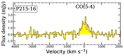
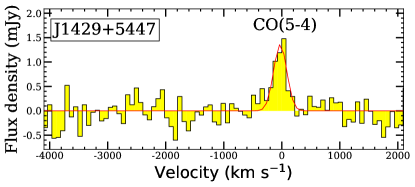
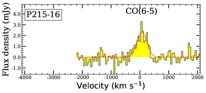
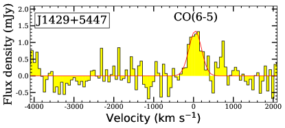
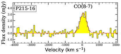
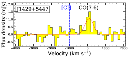
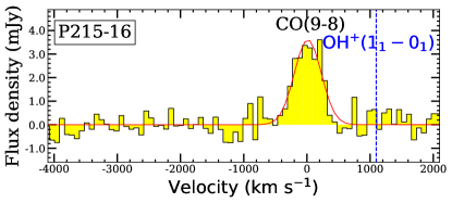
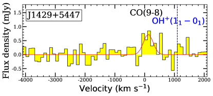
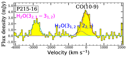
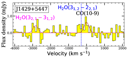
Figure 1: Spectra of the CO, $\rm H_{2}O$, $\rm OH^{+}(1_{1}-0_{1})$, [C I]$(2-1)$ lines for P215$-$16 (left) and J1429+5447 (right). The continuum emission has been subtracted for each of the spectra. The data are shown as yellow histograms. Gaussian profiles fitted to the line emission are shown as solid or dashed lines. The expected positions of the undetected lines are indicated as dashed blue vertical lines. In the spectra where more than one line is detected, the solid black lines represent the sum of different Gaussian components.

As for the quasar J1429+5447, we used three separate executions to cover the CO$(5-4)$, CO$(6-5)$, CO$(7-6)$,[C I]$(2-1)$, CO$(9-8)$, $\rm OH^{+}(1_{1}-0_{1})$, CO$(10-9)$, $\rm H_{2}O(3_{12}-2_{21})$, $\rm H_{2}O(3_{21}-3_{12})$ emission lines, and the underlying continuum emission. The CO$(5-4)$ and the CO$(6-5)$ lines were covered in the LSB and USB, respectively, with one frequency setup, for an on-source time of 3.2 hours. The CO$(9-8)$, $\rm OH^{+}(1_{1}-0_{1})$, CO$(10-9)$, $\rm H_{2}O(3_{12}-2_{21})$, and the $\rm H_{2}O(3_{21}-3_{12})$ emission lines were observed simultaneously in one tuning in the 2 mm band for 2.1 hours on source. Observations of the CO$(7-6)$ and [C I]$(2-1)$ lines were conducted in one frequency setup for 2.2 hours on source. We observed the continuum emission using all line-free channels in the USBs and LSBs in each observation. For all the observations, 1418+546 was used as phase/amplitude calibrator. The fluxes were calibrated with MWC349, 2010+723 and 3C273. The typical calibration uncertainty is $<10\%$ in Band 1 and $<15\%$ in Band 2.

We reduced the data using the CLIC and MAPPING packages that are part of the Grenoble Image and Line Data Analysis System (GILDAS) software (Guilloteau & Lucas, 2000). We obtained the continuum $uv$ tables by averaging all the line-free channels using the UV$\_$AVERAGE task in MAPPING. To generate the continuum subtracted spectral line $uv$ tables, we adopted the continuum $uv$ table obtained above as a continuum model, and use the UV$\_$SUBTRACT task to subtract it from the original $uv$ tables. The $uv$ tables of the spectral lines and the continuum were cleaned and imaged with natural weighting to maximize the S/N ratio (SNR) for point source. The host galaxies are spatially unresolved in beam sizes of $\sim$ 3^′′–6${}^{\prime\prime}\times 1^{\prime\prime}$–2^′′ for P215$-$16 and 2^′′–7${}^{\prime\prime}\times 2^{\prime\prime}$–5^′′ for J1429+5447, respectively. The spectra were finally binned to 46–78 $\rm km\ s^{-1}$ for the quasar P215$-$16 and 45–75 $\rm km\ s^{-1}$ for the quasar J1429+5447. The rms noise for the continuum emission in all bands is 0.02–0.05 mJy $\rm beam^{-1}$ for both sources. Detailed information on the targeted lines and derived parameters can be found in Table 1.

Table 1: Measured emission line and continuum properties

Source	Line	$\nu_{rest}$	$z$	FWHM	S$\delta v$	Luminosity	Beam Size	Channel width
		GHz		(km s-1)	(Jy $\rm km\ s^{-1}$)	($\times 10^{8}\ L_{\sun}$)		($\rm km\ s^{-1}$)
(1)	(2)	(3)	(4)	(5)	(6)	(7)	(8)	(9)
P215$-$16	CO$(5-4)$	576.268	5.7831 $\pm$ 0.0006	444 $\pm$ 63	0.90 $\pm$ 0.17	2.4 $\pm$ 0.5	5$\farcs$74$\times$1$\farcs$73, PA=5°	56
	CO$(6-5)$	691.473	5.7837 $\pm$ 0.0004	404 $\pm$ 42	1.01 $\pm$ 0.14	3.3 $\pm$ 0.5	4$\farcs$82$\times$1$\farcs$45, PA=4°	46
	CO$(8-7)$	921.800	5.7834 $\pm$ 0.0003	443 $\pm$ 39	1.54 $\pm$ 0.18	6.7 $\pm$ 0.8	4$\farcs$45$\times$0$\farcs$92, PA=8°	70
	$\rm OH^{+}(1_{1}-0_{1})$	1033.118	5.7824	503	$<$ 0.57	$<$ 2.7	3$\farcs$14$\times$1$\farcs$09, PA=5°	78
	CO$(9-8)$	1036.912	5.7824 $\pm$ 0.0004	503 $\pm$ 37	1.93 $\pm$ 0.19	9.4 $\pm$ 0.9	3$\farcs$14$\times$1$\farcs$09, PA=5°	78
	CO$(10-9)$	1151.985	5.7824	491$\pm$41	2.00 $\pm$ 0.24	10.8 $\pm$ 3.6	4$\farcs$41$\times$1$\farcs$09, PA=6°	71
	$\rm H_{2}O(3_{12}-2_{21})$	1153.127	5.7824	491$\pm$41	0.42 $\pm$ 0.18	2.2 $\pm$ 0.9	4$\farcs$41$\times$1$\farcs$09, PA=6°	71
	$\rm H_{2}O(3_{21}-3_{12})$	1162.912	5.7824	491$\pm$41	1.32 $\pm$ 0.18	7.2 $\pm$ 2.0	4$\farcs$41$\times$1$\farcs$09, PA=6°	71
J1429+5447	CO$(5-4)$	576.268	6.1824 $\pm$ 0.0005	267 $\pm$ 50	0.39 $\pm$ 0.09	1.2 $\pm$ 0.3	6$\farcs$32$\times$5$\farcs$11, PA=46°	75
	CO$(6-5)$	691.473	6.1841 $\pm$ 0.0007	372 $\pm$ 70	0.53 $\pm$ 0.13	1.9 $\pm$ 0.5	5$\farcs$33$\times$4$\farcs$33, PA=48°	62
	CO$(7-6)$	806.652	6.1841	372	0.48 $\pm$ 0.10	2.0 $\pm$ 0.4	2$\farcs$45$\times$2$\farcs$14, PA=38°	62
	[C I]$(2-1)$	809.342	6.1841	372	$<0.31$	$<1.3$	2$\farcs$45$\times$2$\farcs$14, PA=38°	62
	$\rm OH^{+}(1_{1}-0_{1})$	1033.118	6.1860	271	$<$ 0.21	$<$ 1.1	3$\farcs$85$\times 2$$\farcs$71, PA=51°	50
	CO$(9-8)$	1036.912	6.1860 $\pm$ 0.0012	$271\pm 69$	0.29 $\pm$ 0.07	1.3 $\pm$ 0.4	3$\farcs$85$\times 2$$\farcs$71, PA=51°	50
	CO$(10-9)$	1151.985	6.1860	313 $\pm$ 119	0.21 $\pm$ 0.06	1.2 $\pm$ 0.3	3$\farcs$49$\times 2$$\farcs$44, PA=51°	45
	$\rm H_{2}O(3_{12}-2_{21})$	1153.127	6.1860	313	$<$ 0.18	$<$ 1.1	3$\farcs$49$\times 2$$\farcs$44, PA=51°	45
	$\rm H_{2}O(3_{21}-3_{12})$	1162.912	6.1860	313 $\pm$ 119	$0.15\pm 0.06$	$0.9\pm 0.3$	3$\farcs$49$\times 2$$\farcs$44, PA=51°	45
	Dust continuum properties
	P215$-$16			J1429+5447
$\rm\nu_{cont}$	Flux density	Rms	Ref		$\rm\nu_{cont}$	Flux density	Rms	Ref
GHz	mJy	$\mu$Jy beam-1			GHz	mJy	$\mu$Jy beam-1
(10)	(11)	(12)	(13)		(14)	(15)	(16)	(17)
83.2	0.21 $\pm$ 0.02	21	[1]		82.2	0.15 $\pm$ 0.02	19	[1]
98.6	0.27 $\pm$ 0.02	20	[1]		98.4	0.09 $\pm$ 0.02	20	[1]
138.3	1.38 $\pm$ 0.03	29	[1]		112.4	0.34 $\pm$ 0.05	52	[1]
153.2	1.84 $\pm$ 0.03	33	[1]		144.2	0.32 $\pm$ 0.02	23	[1]
168.4	2.37 $\pm$ 0.05	48	[1]		159.8	0.41 $\pm$ 0.04	35	[1]
352.7	16.85 $\pm$ 1.10	$\cdots$	[2]		1.4	2.68 $\pm$ 0.16	$\cdots$	[3]
666.2	26.93 $\pm$ 7.78	$\cdots$	[2]		3	1.81 $\pm$ 0.11	$\cdots$	[4]
					32	0.26 $\pm$ 0.02	$\cdots$	[5]
					250	3.05 $\pm$ 0.11	$\cdots$	[6]

Note. — Columns 1–2: Source name and line ID. Columns 3–7: Line rest frequency, Redshift, line width in FWHM, flux, and luminosity. Columns 8–9: Beam size and channel width. Columns 10–13 and 14–17: Continuum frequency/wavelength, flux, RMS noise, and references for P215$-$16 and J1429+5447, respectively. References: [1] This work, [2] Li et al. 2020, [3] Villarreal Hernández & Andernach 2018, [4] Becker et al. 1995, [5] Wang et al. 2011 , [6] Khusanova et al. 2022.

3 results

We detect the CO$(5-4)$, CO$(6-5)$, CO$(8-7)$, CO$(9-8)$, CO$(10-9)$, and the $\rm H_{2}O(3_{21}-3_{12})$ lines from the host galaxy of P215$-$16 at SNR $>5$, and report a non-detection of the $\rm OH^{+}(1_{1}-0_{1})$ line (Fig. 1). A tentative detection ($\sim 2.3\sigma$) of the $\rm H_{2}O(3_{12}-2_{21})$ line blended with the CO$(10-9)$ line is also obtained for this object. The continuum emission is detected at SNR ratio $>10$ in all the observed bands (Table 1).We extract the spectra from the peak pixels and fit the spectra of CO$(5-4)$, CO$(6-5)$, CO$(8-7)$, and CO$(9-8)$ lines separately, each with a Gaussian profile. The redshifts and line widths derived for different CO lines are consistent with each other within the uncertainties. The CO$(10-9)$, $\rm H_{2}O(3_{12}-2_{21})$, and $\rm H_{2}O(3_{21}-3_{12})$ lines are covered in the same sideband. We fit these three lines simultaneously, using a Gaussian model, with the line centers fixed to the redshift derived from the CO$(9-8)$ line and an identical line width for all of the three spectral lines (assuming that these three lines are originating from the same gas component). The spectra and the Gaussian fitting results are shown in Fig. 1. Adopting the line width of the CO$(9-8)$ line, we obtain a velocity-integrated map centered at the $\rm OH^{+}(1_{1}-0_{1})$ line frequency and measure the 3$\sigma$ detection upper limit for the $\rm OH^{+}(1_{1}-0_{1})$ line. The measurements for both spectral lines and dust continuum are presented in Table 1.

For the quasar J1429+5447, we detect the CO$(5-4)$, CO$(6-5)$, CO$(7-6)$, and CO$(9-8)$ lines at SNR $>4$, and tentatively detect the CO$(10-9)$ and the $\rm H_{2}O(3_{21}-3_{12})$ lines at the 3.5 and 2.5$\sigma$ levels, respectively. The [C I]$(2-1)$, $\rm H_{2}O(3_{12}-2_{21})$, and $\rm OH^{+}(1_{1}-0_{1})$ lines are undetected (Fig. 1). The CO lines detected in J1429+5447 has lower S/N compared to those detected in P215$-$16. The SNR of the CO$(7-6)$ line spectrum is low. We fix the Gaussian line width and redshift to that of the CO$(6-5)$ line and fit the line flux. The resulting line widths, redshifts, fluxes, and continuum fluxes are listed in Table 1. The $3\sigma$ upper limits of the [C I]$(2-1)$, $\rm OH^{+}(1_{1}-0_{1})$, and $\rm H_{2}O(3_{12}-2_{21})$ lines are estimated based on the rms of the moment 0 maps, which are integrated over channels expected for these lines assuming the same line widths and redshifts as that of their neighboring CO lines. The derived redshifts and line widths of the CO lines are consistent with each other within the uncertainties. These are also consistent with the fitting results of the W component of the CO$(2-1)$ line (the western peak that coincides with the optical quasar) reported in Wang et al. (2011). The continuum emissions are all detected at a $>4\sigma$ level. More details about the measured dust and spectral line properties are listed in Table 1.

4 dust and gas properties

4.1 Dust SED fitting

To derive the dust properties of the two quasars, we analyze their dust spectral energy distributions (SEDs). Optically thick dust model has been suggested to explain the dust emission in a few high-$z$ starburst systems, especially at rest-frame wavelengths $<\sim 200\ \mu$m (e.g., Riechers et al. 2013; Wang et al. 2019). Since the quasars in this work are all far-infrared bright sources, it is reasonable to consider that the dust can be optically thick close to the peak of the dust SED. We thus employ the general opacity dust formula published in da Cunha et al. (2021) to fit the dust SEDs of the quasars in this work. In the general opacity regime, the dust emission can be described by:

$$S_{\nu}\propto[1-{\rm exp(-\tau_{\nu})}](B_{\nu}[T_{\rm dust}(z)]-B_{\nu}[T_{\rm CMB}(z)]),$$ (1)

taking into account the effect of the cosmic microwave background (CMB). Here $B_{\nu}[T_{\rm dust}(z)]$ or $B_{\nu}[T_{\rm CMB}(z)]$ is the Planck function at the temperature of the dust or CMB at the quasar’s redshift, and the dust optical depth $\tau_{\nu}$ is proportional to the dust surface density $\Sigma_{\rm dust}$ via:

$$\tau_{\nu}=\kappa_{\nu}\Sigma_{\rm dust},$$ (2)

where $\kappa_{\nu}$ is the dust opacity. Its dependence on frequency is:

$$\kappa_{\nu}=\kappa_{0}(\frac{\nu}{\nu_{0}})^{\beta},$$ (3)

where $\beta$ is the dust emissivity index and $\kappa_{0}$ is the emissivity of dust grains per unit mass at frequency $\nu_{0}$. If we assume a simple spherical geometry, then the dust mass is:

$$M_{\rm dust}=4\pi R^{2}\Sigma_{\rm dust},$$ (4)

where $R$ is the dust radius of a galaxy. In da Cunha et al. (2021), an additional parameter $\lambda_{\rm thick}$ is introduced, which is defined when the optical depth reaches 1,

$$\tau_{\lambda_{\rm thick}}=1\Longrightarrow\lambda_{\rm thick}=\lambda_{0}(\kappa_{0}\frac{M_{\rm dust}}{4\pi R^{2}})^{1/\beta}.$$ (5)

Accordingly, the dust emission can be rewritten as:

$$S_{\nu}\propto\ [1-{\rm exp(-(\frac{\nu\lambda_{thick}}{\textit{c}})^{\beta})}]\times$$ (6)

$$(B_{\nu}[T_{\rm dust}(z)]-B_{\nu}[T_{\rm CMB}(z)]),$$

where $c$ is the speed of light.

Complemented with SCUBA 2 observations of the dust continuum at 450 $\mu$m (666.2 GHz) and 850 $\mu$m (352.7 GHz) from Li et al. (2020), we use the general opacity model (Eq. 6) to fit the observed dust SED of P215$-$16, normalized to the continuum flux density at 666.2 GHz. Under the general opacity assumption, the dust SED is determined by three parameters: namely $T_{\rm dust}$, $\beta$, and $\lambda_{\rm thick}$. We consider three different dust models. To break the degeneracy between different parameters in dust SED fitting, we fix $\lambda_{\rm thick}$ to (1) the average value of SMGs ($\lambda_{\rm thick}=100\ \mu m$; da Cunha et al. 2021) (Model 1), and (2) the average value of QSOs at $z\sim 6$ ($\lambda_{\rm thick}=264\ \mu m$; derived from Gilli et al. 2022) (Model 2), while enabling $T_{\rm dust}$ and $\beta$ to vary in these two models. In a third model, we enable all three parameters $\lambda_{\rm thick}$, $T_{\rm dust}$, and $\beta$ to vary (Model 3). To explore the posterior distributions of the parameters, we use the Markov Chain Monte Carlo (MCMC) python package emcee to fit the data to the model (Foreman-Mackey et al., 2013), adopting the best-fit values obtained for the least square estimation as educated initial guesses of the parameters.

The inclusion of the high-frequency SCUBA 2 observations is critical in constraining the dust SED parameters for P215$-$16. The least-square estimation finds best-fit values of $T_{\rm dust}=48\rm\ K$, and $\beta=2.05$ for Model 1, $T_{\rm dust}=111\rm\ K$, and $\beta=2.62$ for Model 2, and $T_{\rm dust}=80\rm\ K$, $\beta=2.33$, and $\lambda_{\rm thick}=199\ \mu m$ for Model 3. In some studies, $T_{\rm dust}$, $\beta$ and $\tau_{1900GHz}$ are adopted to describe the general opacity dust SED model (e.g., Walter et al. 2022; Decarli et al. 2023), where $\tau_{1900GHz}$ is the dust optical depth at 1900 GHz. The derived $\lambda_{\rm thick}$ values for our model translate into $\tau_{1900GHz}$ of 0.39, 3.84, and 1.71 for Model 1, 2, and 3, respectively, which is consistent with values derived for other quasars at $z\sim 6$ (Walter et al. 2022; Decarli et al. 2023). By using the MCMC method, we obtain fitting results of $T_{\rm dust}=50^{+6}_{-5}\rm\ K$, and $\beta=1.99^{+0.22}_{-0.22}$, $T_{\rm dust}=116^{+18}_{-11}\rm\ K$, and $\beta=2.53^{+0.37}_{-0.34}$, and $T_{\rm dust}=108^{+47}_{-33}\ \rm K$, $\beta=2.49^{+0.57}_{-0.44}$, and $\lambda_{\rm thick}=252^{+57}_{-65}\ \mu m$ for Model 1, 2, and 3, respectively (see Fig. 2). The derived dust temperature and emissivity index are in agreement with results obtained for other quasars at $z\sim 6$ adopting an optically thick assumption (e.g., Wang et al. 2019; Pensabene et al. 2022), as well as results obtained from 3D radiative transfer calculations (Di Mascia et al., 2021). The resulting infrared (IR, 8 $\mu m-1000\ \mu m$) luminosities ($L_{\rm IR}$) are $1.80^{+0.20}_{-0.20}\times 10^{13}$ $L_{\sun}$, $4.61^{+0.25}_{-0.25}\times 10^{13}$ $L_{\sun}$, and $2.70^{+0.40}_{-0.40}\times 10^{13}$ $L_{\sun}$ for the three models, respectively. If we adopt the previously widely used optically thin modified blackbody dust model for $z\sim 6$ quasars with parameters of $T_{\rm dust}=47\rm\ K$, and $\beta=1.6$ (Beelen et al., 2006), the derived infrared luminosity is 1.9 $\times 10^{13}$ $L_{\sun}$, which is close to the result of Model 1.

J1429+5447 is a radio-loud quasar, we thus also include a power-law radio emission component $f_{\nu}\propto\nu^{\alpha}$, with a power-law index of $\alpha$ to fit the data in addition to the thermal dust SED model (Eq. 6). Besides the continuum emission detected in this paper, we include published continuum data at 1.4, 3 GHz from the Very Large Array Sky Survey (VLASS) and Faint Images of the Radio Sky at Twenty Centimeters (FIRST) (Villarreal Hernández & Andernach 2018; Becker et al. 1995), and 32 and 250 GHz obtained using the Karl Jansky Very Large Array (VLA), and NOEMA (Wang et al. 2011; Khusanova et al. 2022), respectively. The observational data cannot constrain all the model parameters for the radio power-law + general opacity model. We thus fix $\lambda_{\rm thick}=100\mu m$ (typical of SMGs) and explore two cases with different assumptions of $T_{\rm dust}$: namely, 50 K (Model 1) and 100 K (Model 2) representing a typical “cold” and “warm” dust, respectively .

The least square estimation suggests best-fit values of $\alpha=-0.76$, and $\beta=2.95$ for Model 1, and $\alpha=-0.76$, and $\beta=2.66$ for Model 2. The resulting $\tau_{1900GHz}$ are 0.26 and 0.30 for Model 1 and 2, respectively, which are consistent with values derived for other quasars at $z\sim 6$ (Walter et al. 2022; Decarli et al. 2023). The MCMC method finds $\beta=3.02^{+0.50}_{-0.53}$ and $\alpha=-0.76^{+0.04}_{-0.05}$, and $\beta=2.74^{+0.58}_{-0.55}$ and $\alpha=-0.76^{+0.04}_{-0.05}$, for Model 1 and 2, respectively (Fig. 3). The derived infrared luminosities are $6.89^{+0.18}_{-0.18}\times 10^{12}$ $L_{\sun}$ and $3.68^{+0.42}_{-0.42}\times 10^{13}$ $L_{\sun}$ for Model 1 and 2, respectively. If we adopt the widely used modified blackbody dust SED model with parameters of $T_{\rm dust}=47\rm\ K$, and $\beta=1.6$ instead, the infrared luminosity is 9.5 $\times 10^{12}$ $L_{\sun}$.

The derived dust properties of P215$-$16 and J1429+5447 are presented in Table 2. Future high-frequency continuum observations, possibly sampling the peak of the dust SED and/or the Wien tail will be critical to further constrain the dust temperature as well as the IR luminosity.

Figure 2: (a) Dust SED fitting results for P215$-$16. The data are shown as black squares. The Top and bottom axes show the observed and rest continuum frequency. The dust SED is fitted with three general opacity models, and the solid lines represent the models with best-fit values (see Sect. 4.1 for further details). (b–d) Posterior distributions of the model parameters for Model 3, 1 and 2, with the same color as the best-fit models in (a). The 2D contours show the [1, 2]$\sigma$ confidence intervals in the marginalized distributions.

Figure 3: (a) Dust SED fitting results for J1429+5447. The data are shown as black squares. The Top and bottom axes show the observed and rest continuum frequency. The dust SED is fitted with the general opacity dust SED model + radio power-law emission (see Sect. 4.1 for further details). The solid/dashed blue (red) lines represent the best-fit general opacity/radio power-law models for Model 1(2). (b) and (c) Posterior distributions of the model parameters for P215$-$16 (c to e) and J1429+5447, respectively. The color scheme for different models is the same as in panel (a). The 2D contours show the [1, 2]$\sigma$ confidence intervals in the marginalized distributions.

Table 2: Dust SED and CO SLED modeling results

Source	Model	LS Best-fit	MCMC
Dust SED	Model($\lambda_{\rm thick-fixed}$,$T_{\rm dust-fixed}$)
P215$-$16	Model 1($100\mu m$, $\ /$ )	$T_{\rm dust}=48\rm K$, $\beta=2.05$	$T_{\rm dust}=50^{+6}_{-5}\rm K$, $\beta=1.99^{+0.22}_{-0.22}$, $L_{\rm IR}$=$1.80^{+0.20}_{-0.20}\times 10^{13}$ $L_{\sun}$
	Model 2($264\mu m$, $\ /$ )	$T_{\rm dust}=111\rm K$, $\beta=2.62$	$T_{\rm dust}=116^{+18}_{-11}\rm K$, $\beta=2.53^{+0.37}_{-0.34}$, $L_{\rm IR}$=$4.61^{+0.25}_{-0.25}\times 10^{13}$ $L_{\sun}$
	Model 3($\ /$ ,$\ /$ )	$T_{\rm dust}=80\rm K$, $\beta=2.33$, $\lambda_{\rm thick}=199\mu m$	$T_{\rm dust}=108^{+47}_{-33}\rm K$, $\beta=2.49^{+0.57}_{-0.44}$, $\lambda_{\rm thick}=252^{+57}_{-65}\mu m$, $L_{\rm IR}$=$2.70^{+0.40}_{-0.40}\times 10^{13}$ $L_{\sun}$
J1429+5447	Model 1($100\mu m$, $50\rm K$)	$\alpha=-0.76$, $\beta=2.95$	$\beta=3.02^{+0.50}_{-0.53}$, $\alpha=-0.76^{+0.04}_{-0.05}$, $L_{\rm IR}$=$6.89^{+0.18}_{-0.18}\times 10^{12}$ $L_{\sun}$
	Model 2($100\mu m$, $100\rm K$)	$\alpha=-0.76$, $\beta=2.66$	$\beta=2.74^{+0.58}_{-0.55}$, $\alpha=-0.76^{+0.04}_{-0.05}$, $L_{\rm IR}$=$3.68^{+0.42}_{-0.42}\times 10^{13}$ $L_{\sun}$
CO SLED
P215$-$16	PDR	$n(\rm H_{2})$ = $10^{6.0}$,$G_{\rm 0}$ = $10^{6.0}$	$\cdots$
	Extreme PDR	$n(\rm H_{2})$ = $10^{7.1}$,$G_{\rm 0}$ = $10^{7.8}$	$\cdots$
	XDR	$n(\rm H_{2})$ = $10^{4.3}$,$F_{\rm x}$ = $10^{1.1}$	$n(\rm H_{2})$ = $10^{4.7^{+0.8}_{-0.6}}$, $F_{\rm x}$ = $10^{0.87^{+0.6}_{-0.4}}$
J1429+5447	PDR	$n(\rm H_{2})$ = $10^{6.0}$, $G_{\rm 0}$ = $10^{5.4}$	$n(\rm H_{2})$ = $10^{5.8^{+0.7}_{-0.3}}$, $G_{\rm 0}$ = $10^{5.6^{+0.4}_{-0.7}}$
	XDR	$n(\rm H_{2})$ = $10^{3.7}$, $F_{\rm x}$ = $10^{1.5}$	$n(\rm H_{2})$ = $10^{3.8^{+1.1}_{-0.3}}$, $F_{\rm x}$ = $10^{0.33^{+1.4}_{-0.7}}$
	PDR + XDR	PDR: $n(\rm H_{2})$ = $10^{5.1}$, $G_{\rm 0}$ = $10^{4.2}$	$n(\rm H_{2})$ = $10^{5.1^{+0.7}_{-1.1}}$, $G_{\rm 0}$ = $10^{4.2^{+0.4}_{-0.5}}$;
		XDR: $n(\rm H_{2})$ = $10^{4.3}$, $F_{\rm x}$ = $10^{2.0}$	$n(\rm H_{2})$ = $10^{4.4^{+0.9}_{-0.7}}$, $F_{\rm x}$ = $10^{1.3^{+1.4}_{-1.3}}$

Note. — The dust SED and the CO SLED fitting results. “LS Best-fit” represents the best-fit result of the least square method. “MCMC” represents the fitting result of the MCMC method. Model($\lambda_{\rm thick-fixed}$,$T_{\rm dust-fixed}$) represents the model where $\lambda_{\rm thick}$ or $T_{\rm dust}$ is fixed to $\lambda_{\rm thick-fixed}$ or $T_{\rm dust-fixed}$. As for the CO SLED modeling, $n(\rm H_{2})$,$G_{\rm 0}$, and $F_{\rm x}$ are in units of $\rm cm^{-3}$, habing field, and $\rm erg\ s^{-1}\ cm^{-2}$.

4.2 ISM properties

CO SLEDs are sensitive probes of the physical conditions (e.g., temperature, density, and radiation field) of the molecular gas. To derive the physical properties of the molecular gas in the host galaxies of these two quasars, we employ the CO SLED grid models published in Pensabene et al. (2021). These models consider two different gas heating mechanisms, namely a PDR heated by the FUV photons from young massive stars and an XDR heated by the X-ray photons from the AGNs. In the PDR model, the shape of the CO SLED is described by two physical parameters: the gas volume density $n(\rm H_{2})$ and the FUV radiation field strength $G_{\rm 0}$ in Habing field units (1 Habing field corresponds to $\rm 1.6\times 10^{-3}\ erg\ s^{-1}\ cm^{-2}$; Habing 1968). The CO SLED in the XDR model is determined by the gas volume density $n(\rm H_{2})$ and the strength of the X-ray radiation field $F_{\rm x}$ in the unit of $\rm erg\ s^{-1}\ cm^{-2}$. To fully sample the molecular region which has a typical column density of $\textgreater 2\times 10^{22}\ \rm cm^{-2}$ (McKee & Ostriker, 2007), we fix the column density of molecular hydrogen to $10^{23}\ \rm cm^{-2}$ for both sets of the PDR and XDR models. The adopted column density is also consistent with the values derived/adopted for other z$\sim$6 quasars (e.g., Meyer et al. 2022; Decarli et al. 2023). Ranges of $n(\rm H_{2})$, $G_{\rm 0}$, and $F_{\rm x}$ for typical molecular clouds explored in the model grids are $10^{2}-10^{6}\ \rm cm^{-3}$, $10^{1}-10^{6}$ and $10^{-2}-10^{2}\rm\ erg\ s^{-1}\ cm^{-2}$ (Pensabene et al., 2021). We consider two cases for the CO SLED fitting: 1) a single PDR component and 2) an XDR component. The fitting procedure for each case is as follows. Firstly, we use the least square estimation for a first-order estimation of the best-fit values of the parameters. Secondly, we employ the MCMC package emcee to sample the posterior distribution of the parameters while using the best-fit values derived above as educated initial guesses for the parameters (Foreman-Mackey et al., 2013).

We show the fitting results in Fig. 4. The CO SLED of P215$-$16 cannot be fitted with any of our PDR models with $n(\rm H_{2})$ and $G_{\rm 0}$ in the range of $10^{2}-10^{6}\ \rm cm^{-3}$ and $10^{1}-10^{6}$ (Fig. 4(a)), which are typical ranges of the PDR regions in star-forming galaxies, starbursts and AGNs (e.g., Gallerani et al. 2014; Pereira-Santaella et al. 2014; Pensabene et al. 2021; Esposito et al. 2022). To further explore if the data can be fitted with an extreme PDR model, we extend the range of $n(\rm H_{2})$ and $G_{\rm 0}$ parameters of Pensabene et al. (2021) to $10^{2}-10^{8}\ \rm cm^{-3}$ and $10^{1}-10^{8}$, respectively, while using the same set of assumptions in CLOUDY. The results suggest that the data can be fitted with an extreme PDR of $n(\rm H_{2})$ = $10^{7.1}\ \rm cm^{-3}$ and $G_{\rm 0}$ = $10^{7.8}$ (Fig. 4(b)). The CO SLED of P215$-$16 can also be fitted with an XDR model. The least square approximation finds a dense XDR component of $n(\rm H_{2})$ = $10^{4.3}\ \rm cm^{-3}$ illuminated by a radiation field of $F_{\rm x}$ = $10^{1.1}$ $\rm erg\ s^{-1}\ cm^{-2}$. The MCMC analysis finds $n(\rm H_{2})$ = $10^{4.7^{+0.8}_{-0.6}}$ $\rm cm^{-3}$ and $F_{\rm x}$ = $10^{0.87^{+0.6}_{-0.4}}$ $\rm erg\ s^{-1}\ cm^{-2}$ for the XDR model, where values and uncertainties are estimated based on the 50th, 16th, and 84th percentiles of the samples in the marginalized distributions of the parameters. It is also possible that the CO SLED of P215$-$16 is contributed by both PDR and XDR components. However, the current CO SLED measurements are insufficient to constrain the parameters for a PDR+XDR model. Future observations of the high-$J$ ($J\geq 11$) CO lines will be critical to discriminate between different models.

As for J1429+5447, the combination of available [C II]_158μm data with the information on the non-detection of the [C I]$(2-1)$ line from this work enables us to constrain the physical conditions of the atomic gas. The [C II]_158μm/[C I]$(2-1)$ luminosity ratio of $>23$ argues for a PDR origin of the line excitation, as the XDR scenario usually results in a lower line ratio of $\lesssim 10$ (Pensabene et al., 2021). Predictions of the [C II]_158μm/[C I]$(2-1)$ ratio in the PDR model are shown in Fig. 5 (Pensabene et al., 2021). The [C II]_158μm/[C I]$(2-1)$, [C II]_158μm/$L_{\rm IR}$, and [C I]$(2-1)$/$L_{\rm IR}$ ratios indicate a PDR component with parameters in the range of $n(\rm H_{2})$= $10^{3-6}$ $\rm cm^{-3}$ and $G_{\rm 0}$ = $10^{3.7-4.7}$ adopting an $L_{\rm IR}$ value of $6.89^{+0.18}_{-0.18}\times 10^{12}$ $L_{\sun}$ $-$ $3.68^{+0.42}_{-0.42}\times 10^{13}$ $L_{\sun}$. Detections of the CO emission lines complemented with previous CO$(2-1)$ observations (Wang et al., 2011) enable us to constrain, for the first time, the molecular ISM physical conditions of a radio-loud quasar at $z>6$.

We analyze the CO SLED of J1429+5447 following a similar procedure as that of P215$-$16. A single “dense” PDR model illuminated by an intense FUV radiation field is able to reproduce the observational data, with parameters of $n(\rm H_{2})$ = $10^{6.0}\ \rm cm^{-3}$, $G_{\rm 0}$ = $10^{5.4}$. A single XDR model is also able to reproduce the CO SLED with best-fit parameters of $n(\rm H_{2})$ = $10^{3.7}\ \rm cm^{-3}$, $F_{\rm x}$ = $10^{1.5}$ $\rm erg\ s^{-1}\ cm^{-2}$. Using the gas conditions derived from [C II]_158μm, [C I]$(2-1)$ and $L_{\rm IR}$ as a constraint of the PDR component, we also try to fit the CO SLED of J1429+5447 with a PDR + XDR model. This leads to a best-fit result of $n(\rm H_{2})$ = $10^{4.3}$ $\rm cm^{-3}$ and $F_{\rm x}$ = $10^{2.0}$ $\rm erg\ s^{-1}\ cm^{-2}$ for the XDR component, and $n(\rm H_{2})$ = $10^{5.1}$ $\rm cm^{-3}$ and $G_{\rm 0}$ = $10^{4.2}$ for the PDR component. The PDR component contributes to 96$\%$ of the total molecular gas mass in this case. The MCMC method finds best-fit values in the range of $n(\rm H_{2})$ = $10^{5.8^{+0.7}_{-0.3}}$ $\rm cm^{-3}$ and $G_{\rm 0}$ = $10^{5.6^{+0.4}_{-0.7}}$ (PDR model), $n(\rm H_{2})$ = $10^{3.8^{+1.1}_{-0.3}}$ $\rm cm^{-3}$ and $F_{\rm x}$ = $10^{0.33^{+1.4}_{-0.7}}$ $\rm erg\ s^{-1}\ cm^{-2}$ (XDR model), and $n(\rm H_{2})$ = $10^{5.1^{+0.7}_{-1.1}}$ $\rm cm^{-3}$ and $G_{\rm 0}$ = $10^{4.2^{+0.4}_{-0.5}}$, and $n(\rm H_{2})$ = $10^{4.4^{+0.9}_{-0.7}}$ $\rm cm^{-3}$ and $F_{\rm x}$ = $10^{1.3^{+1.4}_{-1.3}}$ $\rm erg\ s^{-1}\ cm^{-2}$ (PDR + XDR model). Analysis of the gas properties using either the [C II]_158μm, [C I]$(2-1)$ and IR ratios or the CO SLED suggests that the [C II]_158μm, [C I]$(2-1)$, CO and IR emission can be explained with one PDR component. However, we are not able to rule out a single XDR model or a composite PDR + XDR model, which reproduces the observed CO SLED. In the case of either XDR or PDR + XDR model, a “moderate density” XDR component illuminated by an intense radiation field is suggested.

Results of the gas properties derived from CO SLED modeling are shown in Table 2. In short, both the extreme-PDR and the XDR model could explain the observed CO SLEDs (up to $J$ = 10) of P215$-$16. However, we also notice that the extreme-PDR model for P215$-$16 requires extremely high gas density and FUV radiation field intensity which is rarely seen in starburst systems and may suggest AGN contribution. For J1429+5447, the CO SLED could be fitted either with a PDR, XDR, or PDR + XDR model. More discussions about the excitation mechanism of the molecular gas can be found in Section 5.

In addition, we robustly detect the $\rm H_{2}O(3_{21}-3_{12})$ line in the quasar P215$-$16, and tentatively detect the $\rm H_{2}O(3_{12}-2_{21})$ in P215$-$16 and $\rm H_{2}O(3_{12}-2_{21})$ and $\rm H_{2}O(3_{21}-3_{12})$ in J1429+5447. The $\rm H_{2}O$ molecule, as the third most abundant species after $\rm H_{2}$ and CO in the molecular ISM phase, traces obscured star formation in dense molecular clouds. Linear relations were reported between the mid/high-$J$ $\rm H_{2}O$ and the IR luminosities in local and high-$z$ infrared bright galaxies and AGNs (e.g., Yang et al. 2013, 2016; Pensabene et al. 2022). The detections and upper limits of $\rm H_{2}O(3_{12}-2_{21})$ and $\rm H_{2}O(3_{21}-3_{12})$ for P215$-$16 and J1429+5447 follow the $\rm H_{2}O$$-$IR trend of other $z\sim 6$ quasars (Yang et al. 2019; Pensabene et al. 2022; Riechers et al. in prep).

Figure 4: CO SLED fitting results of the PDR (left), extreme-PDR (middle), and XDR model (right) for P215$-$16 (top) and PDR (left), XDR (middle), and PDR+XDR (right) model for J1429+5447 (bottom). The fitting results are shown in solid blue (PDR) and red (XDR) lines, and the data are shown in black squares and diamonds for P215$-$16 and J1429+5447, respectively. The sum of the PDR+XDR model is shown as a solid black line.

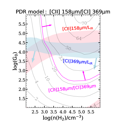
Figure 5: CLOUDY PDR model prediction for the [C II]_158μm/[C I]$(2-1)$ line ratio (grey contours) with different gas density ($\rm n(H_{2})$) and radiation field ($\rm G_{0}$). We also show the value of the [C II]_158μm/$L_{\rm IR}$ ratio (pink region), the lower-limit of the [C II]_158μm/[C I]$(2-1)$ ratio (magenta solid line), and the upper-limit of the [C I]$(2-1)$/$L_{\rm IR}$ ratio (light blue region) for J1429+5447.

5 Discussion: The heating mechanisms of the molecular gas

With the NOEMA observations of the multiple CO transitions, we analyze the CO SLEDs of two $z>5.7$ quasars. Both of them are amongst the most infrared luminous objects found so far in the early Universe. The IR luminosities are of order of a few $10^{12}$ to $10^{13}$ $L_{\sun}$, revealing massive star formation in a dusty ISM. J1429+5447 is a radio-loud quasar, which enables us to study the CO excitation close to a young and radio-loud AGN for the first time.

To further explore the possible origins of the different CO excitations observed in P215$-$16 and J1429+5447, we compare our observations with the CO SLEDs of local and high-$z$ starburst galaxies and AGNs. The results are shown in Fig. 6. The local and high-$z$ galaxy samples are local (ultra-) luminous infrared galaxies (“local (U)LIRGs”; Rosenberg et al. 2015), local star-forming and starburst galaxies (“local SF + SB”; Liu et al. 2015), lensed (sub)millimeter galaxies at $z=2-4$ (“$z=2-4$ SMGs”; Yang et al. 2017), and (sub)millimeter galaxies at $z=1.2-4.1$ (“ $z=1.2-4.1$ SMGs”; Bothwell et al. 2013; Fig. 6a). The representative local galaxies comprise three AGNs, NGC 1068 (Spinoglio et al., 2012), Mrk 231 (van der Werf et al., 2010), and NGC 6240 (Rosenberg et al., 2015), and the starburst galaxy M82 (Weiß et al. 2005; Panuzzo et al. 2010; Fig. 6b). The $z\gtrsim 6$ comparison sources include the $z\sim 6$ quasars that have previous published CO SLEDs with detections of at least four transitions: J2310+1855 (Li et al., 2020a), J1148+5251 (Bertoldi et al. 2003; Walter et al. 2003; Beelen et al. 2006; Riechers et al. 2009; Gallerani et al. 2014), J0100+2802 (Wang et al., 2019), J0439+1634 (Yang et al., 2019), and PJ231–20 (Pensabene et al. 2021; Fig. 6c). As the CO$(6-5)$ line is not observed in PJ231–20, we normalize its CO SLED using the predicted CO$(6-5)$ flux from the best fit radiative transfer model of Pensabene et al. (2021). In addition, we collect starburst galaxies at $z\gtrsim 6$, including SPT 0311 W, SPT 0311 E (Jarugula et al., 2021), and HFLS3 (Riechers et al., 2013), as well a lensed quasar APM 08279 at $z=3.9$ which reveals the highest excited CO SLED ever published across redshifts (Weiß et al. 2007; Bradford et al. 2011; Fig. 6d).

The CO SLEDs of local and high-$z$ starburst galaxy samples typically peak at $J\lesssim 6$, and drop rapidly at high $J$, resulting in low line fluxes at $J>10$ (Fig. 6a). This is consistent with the gas heated by the FUV photons from young massive stars, indicating a PDR origin. On the other hand, the local AGNs and high-$z$ quasars tend to have higher CO excitation with the CO SLEDs peaking at $J\gtrsim 6$. The bright high-$J$ ($J\gtrsim 9$) CO transitions are usually associated with other heating mechanisms, e.g., X-ray heating from AGNs, cosmic ray heating, and mechanical heating by shocks in addition to the FUV heating from young massive stars (Fig. 6b and c; e.g., van der Werf et al. 2010; Spinoglio et al. 2012). As is suggested by Fig. 6 and radiative transfer model predictions, the CO SLEDs of the starburst galaxies and AGNs/quasars are distinguishable through observations of the high-$J$ (e.g., $J\gtrsim 9$) CO transitions (e.g., Vallini et al. 2019).

P215$-$16 exhibits a highly excited CO SLED indicating an excitation level that is much higher than that of all local/high-$z$ starburst galaxies (Fig. 6a and b) and local AGNs (Fig. 6b), with no turn-over up to $J=10$. It has the highest CO$(10-9)$/CO$(6-5)$ ratio among all published quasars at $z\sim 6$ (Fig. 6c) and the second highest excited CO ever across redshifts (less excited compared to APM 08279). We have demonstrated in Section 4.2 that either an XDR component with high gas density and intense radiation ($n(\rm H_{2})$ = $10^{4.3}\ \rm cm^{-3}$, $F_{\rm x}$ = $10^{1.1}$ $\rm erg\ s^{-1}\ cm^{-2}$) or an extreme PDR of $n(\rm H_{2})$ = $10^{7.1}\ \rm cm^{-3}$ and $G_{\rm 0}$ = $10^{7.8}$ could explain such a highly excited CO SLED (Fig. 4). Mechanical heating by shocks can also result in highly excited molecular CO which was reported in some local galaxies (Rosenberg et al., 2015). Shocks are relatively more efficient in heating the gas compared to the dust, and a typical signature of shock-heated gas is a high CO/IR luminosity ratio of a few times $10^{-4}$ (e.g., Pellegrini et al. 2013). The CO/IR ratio (even for the brightest CO$(10-9)$ transition) of P215$-$16 is $\sim 10^{-5}$, which disfavors the shock heating scenario. Enhanced cosmic ray heating could also be responsible for high-$J$ CO line excitation which is sometimes indistinguishable from XDR. Vallini et al. (2019) investigated several CO excitation mechanisms in high-$z$ galaxies and reported that the most extreme cosmic-ray heated CO SLED peaked at $J=9$. The high CO excitation of P215$-$16, which peaks at $J\geq 10$, is best explained by an XDR or extreme-PDR component. In either case, AGN could be the source powering the high CO excitation, by contributing to the X-ray emission or intense FUV emission as suggested by the results of the XDR and extreme-PDR model.

To the contrary, J1429+5447 exhibits a relatively lower CO excitation, which is comparable to that measured for local and high-$z$ starburst galaxies (Fig. 6a and b), and $z\gtrsim 6$ starburst galaxies, e.g., SPT 0311 W, SPT 0311 E, and HFLS3 (Fig. 6d). It has the lowest CO$(J-J$-1)_[J≥7] /CO$(6-5)$ line ratios among the $z\sim 6$ quasars with published CO SLEDs (Fig. 6d). The CO SLED could be explained by a single PDR model with extreme gas densities of $n(\rm H_{2})$ = $10^{6.0}\ \rm cm^{-3}$ and radiation of $G_{\rm 0}$ = $10^{5.4}$.

We also explore if the CO SLED of J1429+5447 can be fitted with an XDR model included, given the luminous X-ray detection in this quasar. The CO SLED of J1429+5447 fitted by an XDR or a PDR+XDR model prefers an XDR component with moderate density ($n(\rm H_{2})$ = $10^{3.7-4.3}\ \rm cm^{-3}$) and illuminated by an intense X-ray radiation field ($F_{\rm x}$ = $10^{1.5-2.0}$ $\rm erg\ s^{-1}\ cm^{-2}$). This is at the lower edge of the molecular gas density range found in $z\sim 6$ quasars (e.g., Li et al. 2020a; Pensabene et al. 2021). As J1429+5447 is a radio-loud object, it is possible that the radio jet expels the gas out of the host galaxy resulting in lower gas density. This is consistent with the indication of a possible outflow found in previous [C II]_158μm observations (Khusanova et al., 2022). The outflowing gas mass constrained from the broad [C II]_158μm component is $1.2\times 10^{10}$ $\rm M_{\sun}$ assuming an $\alpha_{\rm[CII]}=30\rm\ M_{\sun}\ L_{\sun}^{-1}$ (Zanella et al., 2018). The $\rm OH^{+}(1_{1}-0_{1})$ absorption is a sensitive tracer of outflows in galaxies and quasars (e.g., Shao et al. 2022). Unfortunately, the low S/N of our $\rm OH^{+}(1_{1}-0_{1})$ spectrum prevents us from deriving useful constraints on the outflowing molecular gas mass and deeper observations will be needed to obtain an independent estimate. In this work, we only include a simple plane parallel geometry and include no dust torus attenuation. A low CO excitation can be produced in a sophisticated geometry XDR model of high dust attenuation even when the X-ray flux and gas density are high (e.g., Vallini et al. 2019). Future CO SLED observations of more radio-loud quasars will possibly enable us to study if the low excitation is rare/common in the radio-loud population.

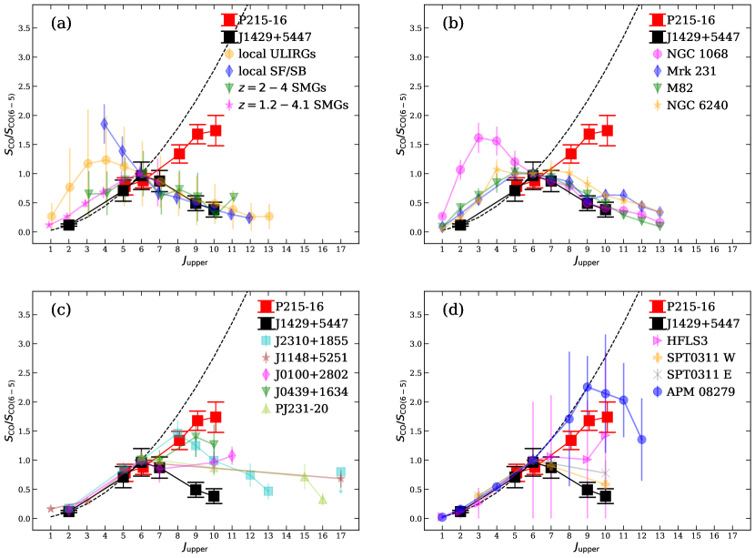
Figure 6: CO SLEDs of P215$-$16 and J1429+5447 in comparison with (a) the mean value of local and high-$z$ starburst galaxy samples, (b) local representative AGNs and starburst galaxies, (c) other quasars at $z\gtrsim 6$, and (d) starburst galaxies at $z\gtrsim 6$ and the lensed quasar APM 08279 at $z=3.9$. The dashed line represents the thermalized CO excitation with constant brightness temperature on the Rayleigh–Jeans scale, i.e., $L^{{}^{\prime}}_{CO(J-J-1)}$ = $L^{{}^{\prime}}_{CO(1-0)}$.

6 Summary

We present NOEMA observations and report detections of multiple CO transitions (from CO$(5-4)$ to CO$(10-9)$), $\rm H_{2}O(3_{21}-3_{12})$ and the underlying continuum emission from the host galaxies of the quasars P215$-$16 at $z=5.78$ and J1429+5447 at $z=6.18$.

Adopting a general opacity dust SED model, we derive dust temperatures in the range of $\sim 50-110\ \rm K$ for the two quasar host galaxies. The derived infrared luminosities of P215$-$16 and J1429+5447 differ by factors of $\sim$ 2.5 and 5.3, respectively, depending on the best-fit models used.

The quasar P215$-$16 exhibits highly excited molecular CO with a CO SLED peaking at $J\geq 10$. It has the highest CO$(J-J$-1)_[J≥7] /CO$(6-5)$ ratio among the $z\sim 6$ quasars with published CO SLEDs known to date. Analysis of the CO SLED with models suggests that a “dense” ($n(\rm H_{2})$ = $10^{4.3}\ \rm cm^{-3}$) XDR component illuminated by an intense X-ray radiation field ($F_{\rm x}$ = $10^{1.1}$) or a “‘dense” PDR component with $n(\rm H_{2})$ = $10^{7.1}\ \rm cm^{-3}$ and $G_{\rm 0}$ = $10^{7.8}$ reproduce the observed CO SLED. In either case, the central AGN is likely to contribute to the radiation field to excite the high$-J$ CO transitions.

The CO SLED of the radio-loud quasar J1429+5447 reveals the lowest CO excitation among all published quasar CO SLEDs at $z\sim 6$. This is the first reported CO SLED of a radio-loud quasar at this redshift and is comparable to those of local AGNs and starburst galaxies at $z\gtrsim 6$. The CO SLED could be explained by a PDR component. In addition, we also propose two possibilities where XDR is considered to explain the low CO excitation: 1) a luminous X-ray radiation field illuminating a moderate-density gas, which may be attributed to a result of the gas expelled by an outflow, and 2) a sophisticated geometry XDR model taking into account the X-ray attenuation by a dust torus. In this case, low CO excitation can be reproduced in a high dust attenuation model even when the X-ray fluxes and gas densities are high.

In addition, we detect bright $\rm H_{2}O(3_{21}-3_{12})$ emission in P215$-$16. This places P215$-$16 exactly on the linear relation between the $\rm H_{2}O(3_{21}-3_{12})$ and IR luminosities recently found for other quasars at $z\sim 6$ and local/high-$z$ infrared bright galaxies.

Future observations of the CO SLEDs towards more radio-loud quasars at $z\gtrsim 6$, possibly up to ($J\gtrsim$ 10) will be critical to systematically reveal the physical conditions and heating mechanisms of the molecular gas in the host galaxies of the radio-loud quasar population in the early universe. Comparisons between the radio-loud and radio-quiet populations will shed light on the possible different/similar impact of the radio-quiet (loud) AGN on the molecular gas properties.

7 acknowledgment

References

- Beelen et al. (2006) Beelen, A., Cox, P., Benford, D. J., et al. 2006, ApJ, 642, 694
- Becker et al. (1995) Becker, R. H., White, R. L., & Helfand, D. J. 1995, ApJ, 450, 559. doi:10.1086/176166
- Bertoldi et al. (2003) Bertoldi, F., Carilli, C. L., Cox, P., et al. 2003, A&A, 406, L55
- Bothwell et al. (2013) Bothwell, M. S., Smail, I., Chapman, S. C., et al. 2013, MNRAS, 429, 3047
- Bradford et al. (2011) Bradford, C. M., Bolatto, A. D., Maloney, P. R., et al. 2011, ApJ, 741, L37. doi:10.1088/2041-8205/741/2/L37
- Carilli & Walter (2013) Carilli, C. L. & Walter, F. 2013, ARA&A, 51, 105. doi:10.1146/annurev-astro-082812-140953
- Circosta et al. (2021) Circosta, C., Mainieri, V., Lamperti, I., et al. 2021, A&A, 646, A96. doi:10.1051/0004-6361/202039270
- da Cunha et al. (2021) da Cunha, E., Hodge, J. A., Casey, C. M., et al. 2021, ApJ, 919, 30. doi:10.3847/1538-4357/ac0ae0
- De Rosa et al. (2014) De Rosa, G., Venemans, B. P., Decarli, R., et al. 2014, ApJ, 790, 145. doi:10.1088/0004-637X/790/2/145
- Decarli et al. (2017) Decarli, R., Walter, F., Venemans, B. P., et al. 2017, Nature, 545, 457. doi:10.1038/nature22358
- Decarli et al. (2018) Decarli, R., Walter, F., Venemans, B. P., et al. 2018, ApJ, 854, 97. doi:10.3847/1538-4357/aaa5aa
- Decarli et al. (2023) Decarli, R., Pensabene, A., Diaz-Santos, T., et al. 2023, A&A, 673, A157. doi:10.1051/0004-6361/202245674
- Di Mascia et al. (2021) Di Mascia, F., Gallerani, S., Behrens, C., et al. 2021, MNRAS, 503, 2349. doi:10.1093/mnras/stab528
- Esposito et al. (2022) Esposito, F., Vallini, L., Pozzi, F., et al. 2022, MNRAS, 512, 686. doi:10.1093/mnras/stac313
- Foreman-Mackey et al. (2013) Foreman-Mackey, D., Hogg, D. W., Lang, D., et al. 2013, PASP, 125, 306. doi:10.1086/670067
- Frey et al. (2011) Frey, S., Paragi, Z., Gurvits, L. I., et al. 2011, arXiv:1105.2371
- Gallerani et al. (2014) Gallerani, S., Ferrara, A., Neri, R., & Maiolino, R. 2014, MNRAS, 445, 2848
- Carniani et al. (2019) Carniani, S., Gallerani, S., Vallini, L., et al. 2019, MNRAS, 489, 3939. doi:10.1093/mnras/stz2410
- Gilli et al. (2022) Gilli, R., Norman, C., Calura, F., et al. 2022, arXiv:2206.03508
- González-Alfonso et al. (2014) González-Alfonso, E., Fischer, J., Aalto, S., et al. 2014, A&A, 567, A91. doi:10.1051/0004-6361/201423980
- Greve et al. (2014) Greve, T. R., Leonidaki, I., Xilouris, E. M., et al. 2014, ApJ, 794, 142. doi:10.1088/0004-637X/794/2/142
- Guilloteau & Lucas (2000) Guilloteau, S. & Lucas, R. 2000, Imaging at Radio through Submillimeter Wavelengths, 217, 299
- Habing (1968) Habing, H. J. 1968, Bull. Astron. Inst. Netherlands, 19, 421
- Jarugula et al. (2021) Jarugula, S., Vieira, J. D., Weiss, A., et al. 2021, ApJ, 921, 97. doi:10.3847/1538-4357/ac21db
- Kamenetzky et al. (2016) Kamenetzky, J., Rangwala, N., Glenn, J., et al. 2016, ApJ, 829, 93. doi:10.3847/0004-637X/829/2/93
- Kawamuro et al. (2020) Kawamuro, T., Izumi, T., Onishi, K., et al. 2020, ApJ, 895, 135. doi:10.3847/1538-4357/ab8b62
- Khusanova et al. (2022) Khusanova, Y., Bañados, E., Mazzucchelli, C., et al. 2022, A&A, 664, A39. doi:10.1051/0004-6361/202243660
- Khorunzhev et al. (2021) Khorunzhev, G. A., Meshcheryakov, A. V., Medvedev, P. S., et al. 2021, Astronomy Letters, 47, 123. doi:10.1134/S1063773721030026
- Kormendy & Ho (2013) Kormendy, J. & Ho, L. C. 2013, ARA&A, 51, 511. doi:10.1146/annurev-astro-082708-101811
- Li et al. (2020) Li, Q., Wang, R., Fan, X., et al. 2020, ApJ, 900, 12. doi:10.3847/1538-4357/aba52d
- Li et al. (2020a) Li, J., Wang, R., Riechers, D., et al. 2020, ApJ, 889, 162. doi:10.3847/1538-4357/ab65fa
- Li et al. (2020b) Li, J., Wang, R., Cox, P., et al. 2020, ApJ, 900, 131. doi:10.3847/1538-4357/ababac
- Liu et al. (2015) Liu, D., Gao, Y., Isaak, K., et al. 2015, ApJ, 810, L14
- Lu et al. (2014) Lu, N., Zhao, Y., Xu, C. K., et al. 2014, ApJ, 787, L23. doi:10.1088/2041-8205/787/2/L23
- McKee & Ostriker (2007) McKee, C. F. & Ostriker, E. C. 2007, ARA&A, 45, 565. doi:10.1146/annurev.astro.45.051806.110602
- Medvedev et al. (2020) Medvedev, P., Sazonov, S., Gilfanov, M., et al. 2020, MNRAS, 497, 1842. doi:10.1093/mnras/staa2051
- Meijerink & Spaans (2005) Meijerink, R. & Spaans, M. 2005, A&A, 436, 397. doi:10.1051/0004-6361:20042398
- Meijerink et al. (2007) Meijerink, R., Spaans, M., & Israel, F. P. 2007, A&A, 461, 793. doi:10.1051/0004-6361:20066130
- Meijerink et al. (2013) Meijerink, R., Kristensen, L. E., Weiß, A., et al. 2013, ApJ, 762, L16. doi:10.1088/2041-8205/762/2/L16
- Meyer et al. (2022) Meyer, R. A., Walter, F., Cicone, C., et al. 2022, ApJ, 927, 152. doi:10.3847/1538-4357/ac4e94
- Migliori et al. (2023) Migliori, G., Siemiginowska, A., Sobolewska, M., et al. 2023, MNRAS, 524, 1087. doi:10.1093/mnras/stad1959
- Mingozzi et al. (2018) Mingozzi, M., Vallini, L., Pozzi, F., et al. 2018, MNRAS, 474, 3640. doi:10.1093/mnras/stx3011
- Montoya Arroyave et al. (2023) Montoya Arroyave, I., Cicone, C., Makroleivaditi, E., et al. 2023, A&A, 673, A13. doi:10.1051/0004-6361/202245046
- Morganson et al. (2012) Morganson, E., De Rosa, G., Decarli, R., et al. 2012, AJ, 143, 142. doi:10.1088/0004-6256/143/6/142
- Panuzzo et al. (2010) Panuzzo, P., Rangwala, N., Rykala, A., et al. 2010, A&A, 518, L37
- Pereira-Santaella et al. (2014) Pereira-Santaella, M., Spinoglio, L., van der Werf, P. P., et al. 2014, A&A, 566, A49. doi:10.1051/0004-6361/201423430
- Pensabene et al. (2020) Pensabene, A., Carniani, S., Perna, M., et al. 2020, A&A, 637, A84. doi:10.1051/0004-6361/201936634
- Pensabene et al. (2021) Pensabene, A., Decarli, R., Bañados, E., et al. 2021, A&A, 652, A66. doi:10.1051/0004-6361/202039696
- Pensabene et al. (2022) Pensabene, A., van der Werf, P., Decarli, R., et al. 2022, A&A, 667, A9. doi:10.1051/0004-6361/202243406
- Pellegrini et al. (2013) Pellegrini, E. W., Smith, J. D., Wolfire, M. G., et al. 2013, ApJ, 779, L19. doi:10.1088/2041-8205/779/2/L19
- Pozzi et al. (2017) Pozzi, F., Vallini, L., Vignali, C., et al. 2017, MNRAS, 470, L64. doi:10.1093/mnrasl/slx077
- Riechers et al. (2006) Riechers, D. A., Walter, F., Carilli, C. L., et al. 2006, ApJ, 650, 604. doi:10.1086/507014
- Riechers et al. (2009) Riechers, D. A., Walter, F., Carilli, C. L., & Lewis, G. F. 2009,ApJ, 690, 463
- Riechers et al. (2011a) Riechers, D. A., Carilli, C. L., Maddalena, R. J., et al. 2011, ApJ, 739, L32. doi:10.1088/2041-8205/739/1/L32
- Riechers (2011b) Riechers, D. A. 2011, ApJ, 730, 108. doi:10.1088/0004-637X/730/2/108
- Riechers et al. (2013) Riechers, D. A., Bradford, C. M., Clements, D. L., et al. 2013, Nature, 496, 329. doi:10.1038/nature12050
- Ramos Almeida et al. (2022) Ramos Almeida, C., Bischetti, M., García-Burillo, S., et al. 2022, A&A, 658, A155. doi:10.1051/0004-6361/202141906
- Rosenberg et al. (2015) Rosenberg, M. J. F., van der Werf, P. P., Aalto, S., et al. 2015, apj, 801, 72
- Ramos Almeida et al. (2022) Ramos Almeida, C., Bischetti, M., García-Burillo, S., et al. 2022, A&A, 658, A155. doi:10.1051/0004-6361/202141906
- Riechers et al. (2013) Riechers, D. A., Bradford, C. M., Clements, D. L., et al. 2013, Nature, 496, 329. doi:10.1038/nature12050
- Shao et al. (2019) Shao, Y., Wang, R., Carilli, C. L., et al. 2019, ApJ, 876, 99. doi:10.3847/1538-4357/ab133d
- Shao et al. (2022) Shao, Y., Wang, R., Weiss, A., et al. 2022, A&A, 668, A121. doi:10.1051/0004-6361/202244610
- Sharon et al. (2016) Sharon, C. E., Riechers, D. A., Hodge, J., et al. 2016, ApJ, 827, 18. doi:10.3847/0004-637X/827/1/18
- Spaans (2008) Spaans, M. 2008, EAS Publications Series, 31, 47. doi:10.1051/eas:0831010
- Spinoglio et al. (2012) Spinoglio, L., Pereira-Santaella, M., Busquet, G., et al. 2012, ApJ, 758, 108
- Uzgil et al. (2016) Uzgil, B. D., Bradford, C. M., Hailey-Dunsheath, S., et al. 2016, ApJ, 832, 209. doi:10.3847/0004-637X/832/2/209
- Valentino et al. (2021) Valentino, F., Daddi, E., Puglisi, A., et al. 2021, A&A, 654, A165. doi:10.1051/0004-6361/202141417
- Vallini et al. (2019) Vallini, L., Tielens, A. G. G. M., Pallottini, A., et al. 2019, MNRAS, 490, 4502. doi:10.1093/mnras/stz2837
- van der Werf et al. (2010) van der Werf, P. P., Isaak, K. G., Meijerink, R., et al. 2010, A&A, 518, L42
- Venemans et al. (2016) Venemans, B. P., Walter, F., Zschaechner, L., et al. 2016, ApJ, 816, 37. doi:10.3847/0004-637X/816/1/37
- Venemans et al. (2018) Venemans, B. P., Decarli, R., Walter, F., et al. 2018, ApJ, 866, 159. doi:10.3847/1538-4357/aadf35
- Venemans et al. (2020) Venemans, B. P., Walter, F., Neeleman, M., et al. 2020, ApJ, 904, 130. doi:10.3847/1538-4357/abc563
- Villarreal Hernández & Andernach (2018) Villarreal Hernández, A. C. & Andernach, H. 2018, arXiv:1808.07178. doi:10.48550/arXiv.1808.07178
- Walter et al. (2003) Walter, F., Bertoldi, F., Carilli, C., et al. 2003, Nature, 424, 406
- Walter et al. (2022) Walter, F., Neeleman, M., Decarli, R., et al. 2022, ApJ, 927, 21. doi:10.3847/1538-4357/ac49e8
- Wang et al. (2008) Wang, R., Carilli, C. L., Wagg, J., et al. 2008, ApJ, 687, 848. doi:10.1086/591076
- Wang et al. (2011) Wang, R., Wagg, J., Carilli, C. L., et al. 2011, ApJ, 739, L34. doi:10.1088/2041-8205/739/1/L34
- Wang et al. (2013) Wang, R., Wagg, J., Carilli, C. L., et al. 2013, ApJ, 773, 44. doi:10.1088/0004-637X/773/1/44
- Wang et al. (2016) Wang, R., Wu, X.-B., Neri, R., et al. 2016, ApJ, 830, 53. doi:10.3847/0004-637X/830/1/53
- Wang et al. (2019) Wang, F., Wang, R., Fan, X., et al. 2019, ApJ, 880, 2. doi:10.3847/1538-4357/ab2717
- Weiß et al. (2005) Weiß, A., Walter, F., & Scoville, N. Z. 2005, A&A, 438, 533
- Weiß et al. (2007) Weiß, A., Downes, D., Neri, R., et al. 2007, A&A, 467, 955. doi:10.1051/0004-6361:20066117
- Willott et al. (2010) Willott, C. J., Delorme, P., Reylé, C., et al. 2010, AJ, 139, 906. doi:10.1088/0004-6256/139/3/906
- Willott et al. (2015) Willott, C. J., Bergeron, J., & Omont, A. 2015, ApJ, 801, 123. doi:10.1088/0004-637X/801/2/123
- Wolfire et al. (2022) Wolfire, M. G., Vallini, L., & Chevance, M. 2022, arXiv:2202.05867
- Yang et al. (2013) Yang, C., Gao, Y., Omont, A., et al. 2013, ApJ, 771, L24. doi:10.1088/2041-8205/771/2/L24
- Yang et al. (2016) Yang, C., Omont, A., Beelen, A., et al. 2016, A&A, 595, A80. doi:10.1051/0004-6361/201628160
- Yang et al. (2017) Yang, C., Omont, A., Beelen, A., et al. 2017, A&A, 608, A144
- Yang et al. (2019) Yang, J., Venemans, B., Wang, F., et al. 2019, ApJ, 880, 153. doi:10.3847/1538-4357/ab2a02
- Zanella et al. (2018) Zanella, A., Daddi, E., Magdis, G., et al. 2018, MNRAS, 481, 1976. doi:10.1093/mnras/sty2394