First spiral arm detection using dynamical mass measurements of the Milky Way disk

We apply the vertical Jeans equation to the Milky Way disk, in order to study non-axisymmetric variations in the thin disk surface density. We divide the disk plane into area cells with a 100 pc grid spacing, and use four separate subsets of the Gaia DR3 stars, defined by cuts in absolute magnitude, reaching distances up to 3 kpc. The vertical Jeans equation is informed by the stellar number density field and the vertical velocity field; for the former, we use maps produced via Gaussian Process regression; for the latter, we use Bayesian Neural Network radial velocity predictions, allowing us to utilize the full power of the Gaia DR3 proper motion sample. For the first time, we find evidence of a spiral arm in the form of an over-density in the dynamically measured disk surface density, detected in all four data samples, which also agrees very well with the spiral arm as traced by stellar age and chemistry. We fit a simple spiral arm model to this feature, and infer a relative over-density of roughly 20 % and a width of roughly 400 pc. We also infer a thin disk surface density scale length of 3.3–4.2 kpc, when restricting the analysis to stars within a distance of 2 kpc.

1 Introduction

In recent years, observations from the Gaia satellite (Gaia Collaboration et al., 2016) have revolutionised our understanding of the structure, history and composition of our Galaxy. Gaia has measured the positions and motions of more than a billion stars, enabling unprecedented analyses of Milky Way stellar dynamics and stellar population properties.

As an example of this progress, many recent studies have sought a better understanding of the spiral structure of the Milky Way (Xu et al., 2018; Shen & Zheng, 2020), which can yield insights into the Galaxy’s formation history. The spiral arms have been probed using various tracers, such as hydrogen gas (Levine et al., 2006), masers (Xu et al., 2013; Reid et al., 2014, 2019), and young stars (Poggio et al., 2021; Castro-Ginard et al., 2021; Lin et al., 2022; Gaia Collaboration et al., 2023a, b). Different studies report slightly different arm morphologies, in terms of pitch angle and spatial extent (e.g., comparing Reid et al. 2019 and Poggio et al. 2021; sometimes such differences can, at least in part, be explained by intrinsic differences between tracers, as discussed by Miyachi et al. 2019). The spiral arms have also been associated with various kinematic signatures (Eilers et al., 2020; Widmark et al., 2022b; Khoperskov & Gerhard, 2022; Martinez-Medina et al., 2022; Palicio et al., 2023).

Despite the aforementioned advances in data precision and depth, the Milky Way’s spiral structure has not previously been detected in a dynamical mass measurement. To detect such variations in the disk surface density requires precise measurements in distant disk regions. This is challenging, mainly because of stellar crowding and dust extinction that cause strong selection effects and other data biases that are difficult to model. Data incompleteness is especially severe for the radial (i.e., line-of-sight) velocity measurements, which are only available for a bright sub-sample of stars.

In the present work, we use state-of-the-art data processing techniques to overcome these obstacles, and perform vertical Jeans analysis of the thin disk out to a distance of 3 kpc from the Sun. Vertical Jeans analysis was formulated a century ago by Jeans (1922), and remains a widely used probe of the dynamical properties of the Solar neighbourhood, such as the local density of dark matter (Sivertsson et al., 2018; Salomon et al., 2020; Guo et al., 2020; de Salas & Widmark, 2021; Widmark et al., 2021a). Under this technique, one assumes dynamical equilibrium and that stellar motions in the directions parallel and perpendicular to the disk plane can be approximately decoupled. Then, a stellar tracer population’s number density distribution and vertical velocity distribution are interrelated via the vertical gravitational potential.

Using the Gaia DR3 catalogue, we construct four separate data samples of bright stars, defined by cuts in absolute magnitude. We divide the disk plane into a square grid with a 100 pc spacing, and apply the vertical Jeans analysis to each such area cell and data sample separately. For the two key ingredients of vertical Jeans analysis, we do the following. For the stellar number density field, we use the 3d maps produced by Widmark et al. (2022b) using Gaussian Processes, based on Gaia and StarHorse spectro-astrometric distances (Anders et al., 2022). For the vertical velocity fields, we use Gaia measurements supplemented by Bayesian Neural Network predictions of radial velocity (i.e., line-of-sight velocity) from Naik & Widmark (2023). These radial velocity predictions are especially useful for our application, because the radial velocity is a sub-dominant component of the vertical velocity in distant regions of the disk, allowing us to make full use of the highly informative Gaia proper motion sample. These data products, in combination, allow us to make a detailed map of how the surface density varies in the directions parallel to the Galactic plane.

For the first time, we find evidence for the imprint of spiral structure in the dynamically measured vertical gravitational potential of the Milky Way disk. In all of our four data samples, we see the same non-axisymmetric over-density, which also agrees very well with the Local Arm as traced by stellar age and chemistry (e.g. Poggio et al. 2021).

2 Method

2.1 Coordinate system and data samples

We use Solar rest-frame Cartesian coordinates $\boldsymbol{X}=(X,Y,Z)$ pointing in the directions of the Galactic centre, Galactic rotation, and Galactic north. The vertical coordinate in the disk frame is equal to

$$z=Z+Z_{\odot},$$ (1)

where $Z_{\odot}$ is the height of the Sun with respect to the Galactic disk mid-plane. The vertical velocity in the Solar rest-frame is $W\equiv\text{d}Z/\text{d}t$. The Galactocentric radius is given by

$$R=\sqrt{(R_{\odot}-X)^{2}+Y^{2}},$$ (2)

where we take $R_{\odot}=8.2\leavevmode\nobreak\ \text{kpc}$ (McMillan, 2016). The Galactocentric angle $\phi$ fulfils

$$\sin\phi=\frac{Y}{R},\quad\cos\phi=\frac{R_{\odot}-X}{R}.$$ (3)

We construct four separate stellar samples by making cuts in Gaia $G$-band absolute magnitude, according to $M_{G}\in(0,1],\,(1,2],\,(2,3]$, and $(3,4]$ (the same as in Widmark et al. 2022b). We divide the $(X,Y)$-plane into a square grid with a cell spacing of 100 pc, for the spatial volume within $\sqrt{X^{2}+Y^{2}}<3\leavevmode\nobreak\ \text{kpc}$.

2.2 Vertical Jeans analysis

The vertical Jeans equation gives

$$\frac{1}{n}\frac{\partial(n\sigma^{2}_{W})}{\partial Z}+\frac{\partial\Phi}{\partial Z}=0,$$ (4)

where $\Phi$ is the gravitational potential, $n$ and $\sigma_{W}^{2}$ are the number density and vertical velocity variance of a stellar tracer population, and $Z$ is the direction perpendicular to the Galactic plane.

In the equation above, we have made a few simplifying assumptions. In particular, we have assumed dynamical equilibrium and dropped a term representing a coupling between radial and vertical motions (the ‘tilt’ term), which gives a sizable contribution only at heights closer to 1 kpc (Read, 2014).

2.3 Stellar number density field

For the stellar number count density, we use the results from Widmark et al. (2022b), where the stellar number density fields of the four data samples were modelled with Gaussian Process (GP) regression. This was based on StarHorse spectro-astrometric distances (Anders et al., 2022), using data from Gaia DR3 (Gaia Collaboration et al., 2023c), Pan-STARRS1 (Scolnic et al., 2015), SkyMapper (Casagrande et al., 2019), 2MASS (Skrutskie et al., 2006), and AllWISE (Marrese et al., 2019). Spatial volumes were carefully masked to avoid open clusters and incompleteness issues associated with dust extinction. By using GPs, the stellar number density field was modelled as a smooth and differentiable function. This approach was also fairly model-independent, and did not impose constraints such as Galactic axisymmetry.

The GP regression used correlation lengths of $(l_{X},l_{Y},l_{Z})=(300,300,100)\leavevmode\nobreak\ \text{pc}$, which imposes a degree of smoothness in all three spatial directions. In this manner, even though the area cells have a 100 pc spacing in $(X,Y)$-plane, the number density field is informed by a larger area. This is especially useful when a larger fraction of an area cell is masked (e.g., due to an open cluster); in that case, its number density field is still informed by the data in its surrounding spatial volume. However, in order to avoid area cells that are very poorly sampled, we mask area cells that have an average effective volume fraction smaller than 0.5 for $|Z|<250\leavevmode\nobreak\ \text{pc}$.

We want to retain the useful properties of GP regression discussed above. However, there are time-varying perturbations to the stellar number population (which the GP regression encapsulates); such perturbations can create a biases in dynamical mass measurements, since they are not in a steady state. Therefore, we fit an analytic function to the stellar number density that was obtained via GP regression, separately for each data sample and area cell, assuming a functional form which is mirror symmetry and monotonically decreasing with height. This analytic function is a mixture model of three disk components, according to

$$\hat{n}(Z\,|\,a_{i},h_{i},Z_{\odot})=\sum_{i=1}^{3}a_{i}\times\text{cosh}^{-2}\left(\frac{Z+Z_{\odot}}{h_{i}}\right),$$ (5)

where $a_{i}$ are the disk component normalisations, $h_{i}$ are the scale heights, and $Z_{\odot}$ is the height of the Sun with respect to the disk mid-plane. This functional form is flexible enough to faithfully model the vertical number density profile of our stellar tracer populations. We use wide flat box priors and the GP regression uncertainties in our fit.

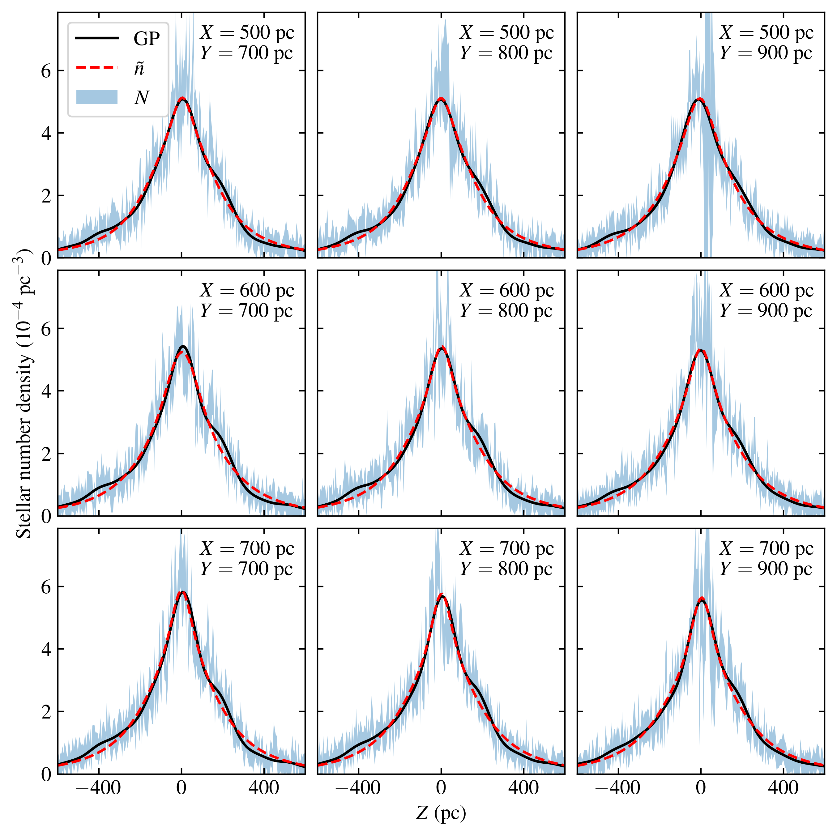
Figure 1: Stellar number density distribution for a few area cells of the data sample with $2<M_{G}\leq 3$. Each panel is labelled by the area cell’s mid-point $(X,Y)$-coordinates. The function obtained by GP regression is shown in solid black; the fitted symmetric function ($\hat{n}$) of Eq. 5 is shown in dashed red; the raw number count ($N$) with its associated Poisson noise uncertainty is shown as a 1$\sigma$ band.

In Fig. 1, we show an example of the stellar number density distribution, in terms of the underlying data counts, GP regression, and symmetric analytic function. We do so for a small area of nine neighbouring area cells of the $2<M_{G}\leq 3$ data sample. We chose this particular spatial volume in order to illustrate a few important features. In the top right panel, the raw data number count has a very large uncertainty, due to open cluster masking. The GP curve is still inferred there, informed by its surrounding spatial volume. In all panels, the stellar over-densities at roughly $Z=200\leavevmode\nobreak\ \text{pc}$ and $Z=-400\leavevmode\nobreak\ \text{pc}$ (and their mirrored under-densities) are projections of the phase space spiral (see figure 7 in Widmark et al. 2022b). Because the phase-space spiral is a time-varying structure, it constitutes a bias to Jeans analysis, which we average away by fitting the symmetric and analytic function $\hat{n}$.

2.4 Vertical velocity field

For the vertical velocity field, we use all Gaia DR3 stars in the unmasked $(X,Y)$ area cells, subdivided into the four data samples. We remove possible (probability $>0.1$) members of the open clusters tabulated by Hunt & Reffert (2023) and stars with StarHorse distance precisions worse than 10%. This leaves 23 551 383 stars overall: 3 262 301, 2 736 077, 5 710 148, 11 842 857 in each of the four magnitude bins, from brightest to faintest.

Of these stars, around 60% have radial velocity measurements in Gaia DR3 (ranging from 85% in the brightest sample to 50% in the faintest). For the remainder of the stars, we use the Bayesian radial velocity predictions of Naik & Widmark (2023). These prediction posterior distributions are generated using Bayesian neural networks (BNNs), trained on the subset of DR3 stars with radial velocities (Naik & Widmark, 2022, 2023). In effect, these BNNs learn a latent representation of the stellar phase space distribution, convolved with any uncertainty due to a lack of training data. As a result, these prediction distributions can be rather wide, with typical widths in the range 20-30 km/s.

In order to account for the uncertainties associated with these predictions, we use the technique of multiple imputation (Little & Rubin, 2014; Gelman et al., 2004). For each star without a radial velocity measurement, we generate 20 realisations from the prediction posterior distributions, and combine these to construct 20 separate datasets (or ‘imputations’). We then conduct the remainder of our analysis separately for each imputation, so that the cross-imputation variation in the final results gives an estimate of the uncertainty due to the missing data.

For each imputation, data sample, and area cell, we convert the measured phase space coordinates (sky positions, StarHorse distances, proper motions, and radial velocities) to the heliocentric Cartesian coordinate system described above. We then fit a parametric model describing $\sigma^{2}_{W}$ as a function of $Z$, using the data of the area cell as well as all adjacent unmasked cells (effectively smoothing our results over a 300-by-300 pc area):

$$\hat{\sigma}^{2}_{W}(Z)=\sigma^{2}_{0}+\sigma^{2}_{1}\ln\left[1+\left(\frac{Z+Z_{\odot}}{H_{1}}\right)^{2}\right]+\sigma^{2}_{2}\ln\left[1+\left(\frac{Z+Z_{\odot}}{H_{2}}\right)^{2}\right],$$ (6)

where $\sigma^{2}_{\{0,1,2\}}$ and $H_{\{1,2\}}$ are dimensionful free parameters in the fit. The quantity $Z_{\odot}$ represents the height of the Sun with respect to the disk mid-plane; this is not taken as a free parameter but as a constant, given by the fit of the stellar number density model in that area cell. We fit the velocity variance model (Eq. 6) to the data $\mathcal{D}$ (comprising stellar heights $Z$, vertical velocities $W$, and observational vertical velocity uncertainties $\sigma_{\mathrm{obs}}$ propagated from proper motion and distance measurements) by maximising a Gaussian log-likelihood,

$$\ln\mathcal{L}(\mathcal{D}\,|\,\overline{W},\sigma^{2}_{\{0,1,2\}},H_{\{1,2\}})=-\frac{1}{2}\sum_{i}\left[\frac{(W_{i}-\overline{W})^{2}}{\sigma_{i}^{2}}+\ln\left(2\pi\sigma_{i}^{2}\right)\right],$$ (7)

where the index $i$ runs over individual stars, and

$$\sigma_{i}^{2}\equiv\sigma_{\mathrm{obs},i}^{2}+\hat{\sigma}^{2}_{W}(Z_{i}|\sigma^{2}_{\{0,1,2\}},H_{\{1,2\}}).$$ (8)

The mean vertical velocity $\overline{W}$ is a sixth free parameter, in addition to the five free parameters $\sigma^{2}_{\{0,1,2\}},H_{\{1,2\}}$ entering the dispersion model.

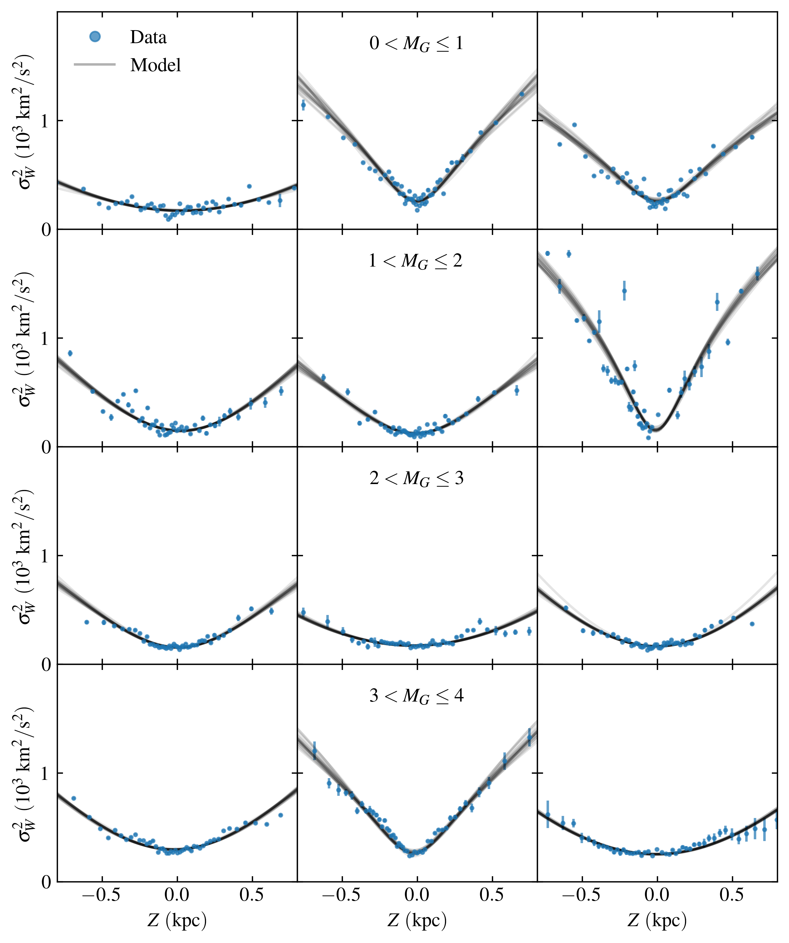
Figure 2: Examples of vertical velocity dispersions and the best-fitting models (Eq. 6). The four rows correspond to the four magnitude samples, while the three panels within each row are randomly chosen cells in $(X,Y)$-plane. The yellow points represent the measured velocity dispersions in adaptively spaced $Z$ bins, while the solid lines show the best-fitting models. Note that the model is not fit to these binned dispersions, but to the individual stellar velocities. In each case, 20 sets of data and 20 models are shown, corresponding to the 20 random imputations of the dataset as described in the main text.

Figure 2 shows a few examples of fitted velocity dispersion profiles. For each of the four data samples, we choose three random area cells and plot the best-fit model according to Eq. 6, as well as the measured velocity dispersions in adaptively spaced vertical bins. In each case, we individually plot the data and model for each of the 20 imputations. It is clear from this figure that our model (Eq. 6) effectively captures the overall shape of the dispersion profiles despite the observed variability in these shapes, while at the same time foregoing smaller-scale features arising from unmixed phase space substructures.

We also tried different models for the vertical velocity dispersion as a function of height. Another functional that gave rise to consistent results (in terms of agreement between different spatial regions and between data sample) was a quartic polynomial. These fits to the velocity data were somewhat worse in terms of $\chi^{2}$-value and by-eye inspection, but we saw very similar results for the inferred gravitational potential, leading to the same general conclusions.

The uncertainties associated with the velocity distribution are dominant in terms of the inferred gravitational potential. These uncertainties are propagated to the global fits of the exponential function and the simple arm models (see Sect. 3).

3 Results

Our dynamical mass measurement is likely the most robust for the potential difference of roughly $\Phi(400\leavevmode\nobreak\ \text{pc})-\Phi(0\leavevmode\nobreak\ \text{pc})$. Between these heights, the stellar number density ratio is roughly 10–15 % for the three brighter data samples, and 30 % for the dimmest data sample. Furthermore, the spiral arms are a thin disk phenomenon; staying closer to the Galactic plane makes the measurement more local and will better resolve the spiral arms, as the gravitational potential at greater heights is influenced by a larger area of the Galactic disk. This potential difference is a good proxy for and closely proportional to the thin disk surface density, which is discussed in Sect. 2.2.

Figure 3 shows our inferred values of $\Phi(400\leavevmode\nobreak\ \text{pc})-\Phi(0\leavevmode\nobreak\ \text{pc})$ as a function of Galactocentric radius, for all four data samples. The markers each correspond to an area cell, where the colour denotes their Galactocentric angle $\phi$. Coherent structure visible in the marker colours (denoting Galactocentric angle $\phi$) reveal non-axisymmetric structure in the inferred surface density results; for example, at the Solar radius ($R=8.2\leavevmode\nobreak\ \text{kpc}$) the results for positive $\phi$ are over-dense compared to negative $\phi$, in all four data samples. We also show an exponential function fitted separately to each data sample, which takes the form

$$f(R)=A\times\exp\left(\frac{R-R_{\odot}}{h_{L}}\right),$$ (9)

where $A$ is the Solar radius value, and $h_{L}$ is the disk scale length parameter. The data samples that are more distant ($\sqrt{X^{2}+Y^{2}}>2\leavevmode\nobreak\ \text{kpc}$) are likely less reliable and therefore masked in this fit. The fitted exponential function parameter values are listed in the respective panels of Fig. 3 and they agree well between the four data samples. We show only the best fit value; the statistical error is small and systematic uncertainties dominate.

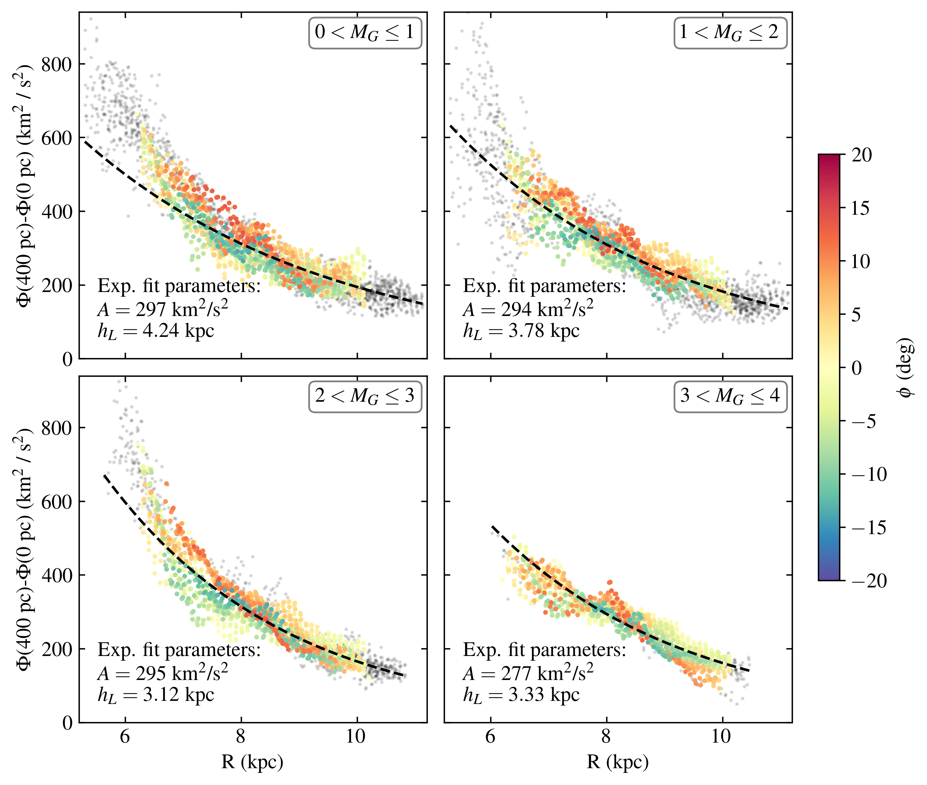
Figure 3: Gravitational potential, $\Phi(400\leavevmode\nobreak\ \text{pc})-\Phi(0\leavevmode\nobreak\ \text{pc})$, as a function of Galactocentric radius, for the four stellar samples (as labelled in the panels’ top right corner). The dashed line is the exponential function of Eq. (9), fitted to data points with $\sqrt{X^{2}+Y^{2}}<2\leavevmode\nobreak\ \text{kpc}$, which excludes distant and dubious spatial regions. The scatter points correspond to area cells in the $(X,Y)$-plane. Area cells that are included in the exponential function fit are coloured according to their Galactocentric disk plane angle ($\phi$); excluded data cells have light grey and smaller scatter points. The colour bar and axis ranges are shared between all panels.

The residual of the inferred $\Phi(400\leavevmode\nobreak\ \text{pc})-\Phi(0\leavevmode\nobreak\ \text{pc})$ as compared to the fitted exponential function is shown in Fig. 4, for all four data samples. The residual of an area cell is defined according to

$$\text{residual}=\frac{\text{measurement}-f(R)}{f(R)},$$ (10)

where $f(R)$ is the fitted exponential function. The residuals of the four data samples show similar results. Most notably, they have the same over-dense structure, stretching roughly from $(X,Y)=(0,1.5)\leavevmode\nobreak\ \text{kpc}$ to $(X,Y)=(-1.5,-0.5)\leavevmode\nobreak\ \text{kpc}$. This feature agrees well with the Local Arm revealed in the map of young stars by Poggio et al. (2021), shown in detail in Fig. 5 and as grey contour lines in Fig. 4.

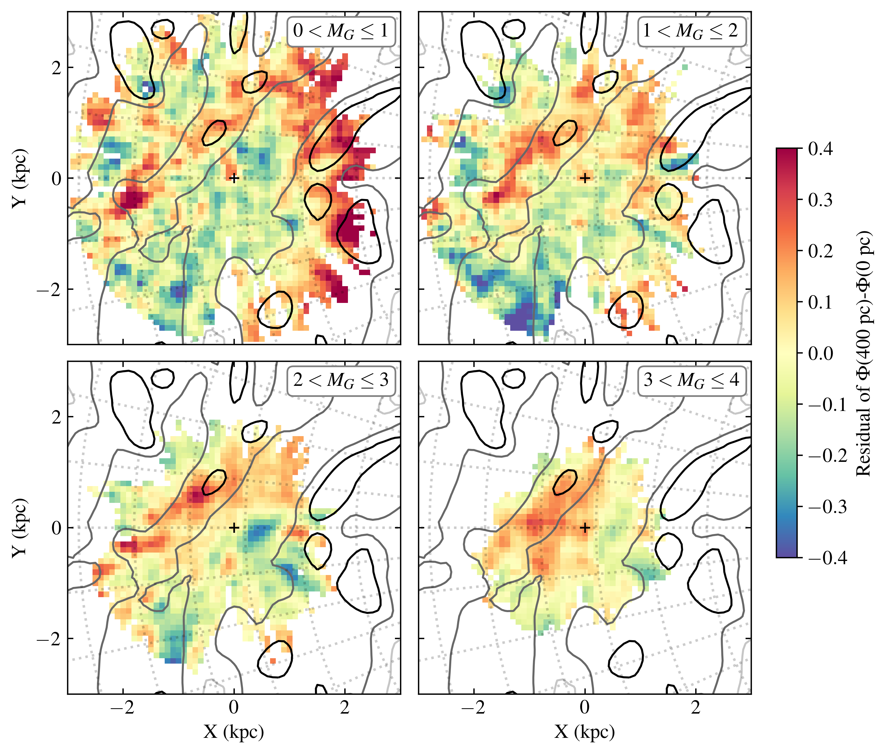
Figure 4: Residual of $\Phi(400\leavevmode\nobreak\ \text{pc})-\Phi(0\leavevmode\nobreak\ \text{pc})$ with respect to a fitted exponential, projected on the $(X,Y)$-plane, where each panel corresponds to one of our four data samples. In each panel, dotted grey lines show Galactocentric iso-radial and iso-azimuthal lines, and the black plus sign in the center marks the Solar position. The grey contour lines correspond to the spiral arms as mapped by Poggio et al. (2021), as seen in Fig. 5.

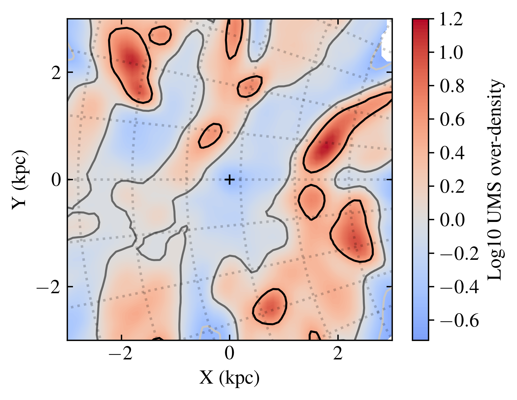
Figure 5: Over-density of upper main sequence stars in the $(X,Y)$-plane, as a tracer of spiral arms. Results are taken directly from Poggio et al. (2021). The grey-scale contour lines are the same as in Fig. 4, corresponding to values $(-0.5,\,0,\,0.5)$.

In order to make quantitative statements about the over-density that we identify with the Local Arm, we fit a simple analytic model to the residual seen in Fig. 4. We model the ridge of the over-density as a 1d curve in the Galactic disk plane, as a logarithmic spiral of the form

$$\tilde{R}(\phi)=\tilde{R}_{0}\exp\left[-\phi\tan(\tilde{\alpha})\right],$$ (11)

where $\tilde{R}_{0}$ is the Galactocentric radius where the arm crosses the $X$-axis (i.e., $\phi=0$), and $\tilde{\alpha}$ is the pitch angle. The relative density in this model is given by the disk plane projected distance to the ridge, according to

$$\text{residual}(R,\phi)=\tilde{a}+\tilde{b}\exp\left\{-\frac{[R-\tilde{R}(\phi)]^{2}\cos^{2}(\tilde{\alpha})}{2\tilde{L}^{2}}\right\},$$ (12)

where $\tilde{a}$ and $\tilde{b}$ are the residual base-line and spiral arm amplitudes, and $\tilde{L}$ is the spiral arm width.

The residuals have some strong outliers; for this reason, we use the 1-norm in our fit (minimising $|\text{data}-\text{model}|$, instead of $|\text{data}-\text{model}|^{2}$), which also gives somewhat more consistent results between data samples. Additionally, we perform a joint fit of all four data samples, which is probably more robust and less prone to over-fitting. The fitted models are shown in Fig. 6, and the parameter values are listed in Table 1. The relative amplitudes of the arm over-density fall in the range of 18–24 %, while the joint fit gives 20 %. The fitted pitch angle is roughly 50^∘–60^∘, which is large compared to typical values in the literature (Levine et al., 2006; Vallée, 2005, 2017). However, our value is likely only applicable to the very local area of study (e.g., similar to the high pitch angle segment of the Sagittarius Arm analysed by Kuhn et al. 2021). The arm width of the joint fit is 0.4 kpc.

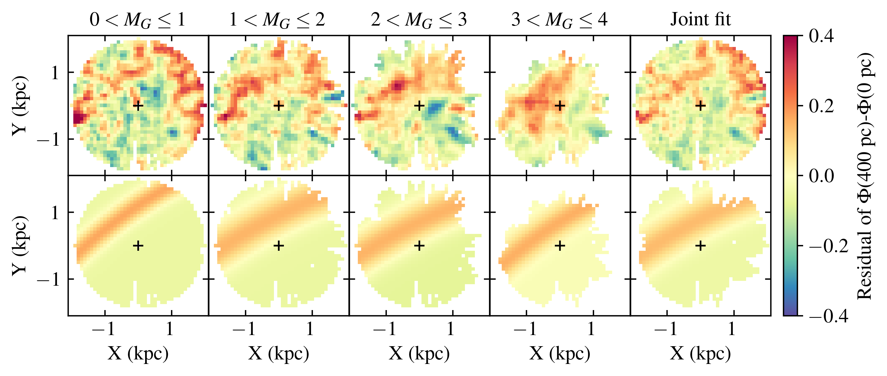
Figure 6: Simple spiral arm model, fitted to the residual of $\Phi(400\leavevmode\nobreak\ \text{pc})-\Phi(0\leavevmode\nobreak\ \text{pc})$, for non-masked area cells within a distance of 2 kpc.

Table 1: Fitted parameters of the simple spiral arm over-density model, as described in Eqs. (11) and (12), for each of the four data samples. The final row is a combination of the $\tilde{a}$ and $\tilde{b}$ parameters, and corresponds to the peak relative over-density as compared to the disk areas far from the spiral arm.

	$\tilde{\alpha}$ (deg)	$\tilde{R}_{0}$ (kpc)	$\tilde{L}$ (kpc)	$\tilde{a}$	$\tilde{b}$	$\tilde{b}/(1+\tilde{a})$
$0<M_{G}\leq 1$	48.2	9.77	0.26	–0.057	0.224	0.24
$1<M_{G}\leq 2$	57.0	9.81	0.44	–0.059	0.206	0.22
$2<M_{G}\leq 3$	59.1	9.52	0.43	–0.075	0.224	0.24
$3<M_{G}\leq 4$	52.5	9.24	0.30	–0.017	0.173	0.18
Joint fit	57.0	9.58	0.38	–0.053	0.190	0.20

4 Discussion

Using vertical Jeans analysis and state-of-the-art data processing, we have produced 2d maps of the thin disk surface density within a distance of 3 kpc of the Sun. Overall, the results of our four data samples agree well. We see the same general over-dense feature in all data samples, and they also agree well with spiral arm tracers based on stellar age and metallicity.

We fitted a simple axisymmetric model to our results, as defined in Eq. (9). The inferred values for normalisation constant (parameter $A$) agree well with previous results for the immediate Solar neighbourhood (Schutz et al., 2018; Widmark et al., 2021a, b). The inferred thin disk scale lengths (parameter $h_{L}$) fall in range 3.3–4.2 kpc. This quantity varies in previous studies: a review from 2016 by Bland-Hawthorn & Gerhard (2016) summarizes 15 articles to give $2.6\pm 0.5\leavevmode\nobreak\ \text{kpc}$; later analyses include $2.2\pm 0.1\leavevmode\nobreak\ \text{kpc}$ (Widmark et al., 2022a), $2.4\pm 0.1\leavevmode\nobreak\ \text{kpc}$ (Wang et al., 2022), roughly 3.9 kpc (Robin et al., 2022), and $2.17^{+0.18}_{-0.08}\leavevmode\nobreak\ \text{kpc}$ (Ibata et al., 2023). An explanation for these discrepancies could be variations in the studied tracer samples and spatial volumes; this could give rise to different results if axisymmetry is broken or if the disk scale length is not constant with respect to $R$. In our own results, the masked data cells at low Galactocentric radii ($R\lesssim 7\leavevmode\nobreak\ \text{kpc}$) seem to follow a steeper profile, likely better described by a broken exponential function. However, we refrain from making a more definite or quantitative statement about this, since our results are quite discrepant beyond 2 kpc and potentially affected by systematic biases, especially towards the Galactic center. The data sample with $1<M_{G}\leq 2$ seems particularly discrepant at low $R$; this data sample has the lowest number count, which likely makes it more prone to systematic errors (how such errors operate is very complicated considering the underlying data processing and how it is affected by low statistics, e.g., the spectro-photometric distances affected by dust extinction, which is especially severe at low $R$).

We have detected the Local Arm in our thin disk surface density measurements, as revealed by the residual maps in Fig. 4, and we can compare and distinguish between other recent probes of the Local Arm morphology. The Local Arm model by Reid et al. (2019), based on masers as a tracer, is somewhat discrepant with recent observations of young star tracers (see figure 5 in Poggio et al. 2021 for a direct comparison with Gaia Collaboration et al. 2023a, b). In the former, the Local Arm barely extends into negative $X$; instead, the outer Perseus Arm has a low pitch angle and curves through $(X,Y)\simeq(-2,-2)\leavevmode\nobreak\ \text{kpc}$. In the latter, the Local Arm has a higher pitch angle, at least in the local area at positive $Y$, and also extends into negative $X$ and $Y$, passing through $(X,Y)\simeq(-2,-2)\leavevmode\nobreak\ \text{kpc}$. Our own results favor the latter Local Arm morphology with a higher pitch angle. However, we do not see evidence for a Local Arm over-density that continues all the way to $(X,Y)\simeq(-2,-2)\leavevmode\nobreak\ \text{kpc}$, as traced by Poggio et al. (2021), although we repeat that our results could be less accurate in spatial volumes beyond roughly 2 kpc.

There are some discrepancies in the inferred surface density of the four data samples, best seen in Fig. 4, in addition to the general arm-like structure. This noise is larger than can be accounted for by statistical uncertainties, which is indicative of some uncontrolled systematic errors. For example, there are small outlier ares, for example close to $(X,Y)\simeq(-2,-0.4)\leavevmode\nobreak\ \text{kpc}$ for the brightest data sample, and the arm-like over-density is closer to the solar position for the dimmest data sample. Systematic errors could arise in the data or in the data processing itself; for example, there is a very complicated interplay with the dust extinction field and the spectro-astrometric distance estimates from StarHorse. There could also be more physical reasons that could bias our results, having to do with the dynamical properties of the respective data samples. For example, the dimmest data sample has a greater spatial scale height and is kinematically hotter; around the solar position, its $u$ and $v$ velocity dispersions are 10–25 % higher, and its vertical velocity dispersion is 20–50 % higher, as compared to the other three data samples. These properties make the data sample sensitive to a larger area of the disk plane’s mass density distribution, and also affects its sensitivity to biases that can arise from a broken equilibrium assumption; for example, the response of a stellar population with respect to a disk vibrational mode can depend on the scale height and kinematic temperature of that stellar population. In fact, Widmark et al. (2022b) found evidence of a breathing mode associated to the local spiral arm (see their figures 9 and 10, for stars with $|z|<300\leavevmode\nobreak\ \text{pc}$), seen in both the stellar number density and vertical velocity distributions; they found a contracting breathing mode (net motion towards the mid-plane) in the inner part of the arm, offset by roughly a quarter wavelength with respect to the arm’s stellar over-density, which is indicative a breathing mode that is travelling against the direction of Galactic rotation.

Despite these systematic errors, our general results are robust. A scenario where the detected Local Arm over-density is caused by data systematics seems extremely contrived, since it is observed over a range of viewing angles, distances, and across four independent data samples. Furthermore, the data samples are quite different in age and small-scale structure; especially the stars of the dimmest data sample are older, kinematically hotter and more smoothly distributed, and do not trace the spiral arms (at least not in a significant manner). The detection of the spiral arm imprint in these data samples is thus not because of the stellar number counts themselves, but because of the gravitational influence that the spiral arms have on the stellar motions.

5 Conclusion

We have applied the vertical Jeans equation to the Milky Way disk, dividing the disk plane into a square grid with a grid spacing of 100 pc, in order to study the thin disk surface density and its spatial dependence along the Galactic plane. We reach distances of a few kilo-parsecs, enabled by state-of-the-art data processing, utilising spectro-photometric distance measurements, GP regression on the stellar number density field, and radial velocity predictions from Bayesian Neural Networks. Specifically, we measure the gravitational potential difference between the disk mid-plane and a height of 400 pc, which serves as a close proxy for the thin disk surface density.

For the first time, we see dynamically measured evidence for an over-density associated with a nearby spiral arm. This over-density is detected in all of our four data samples (defined by cuts in absolute magnitude), with a relative amplitude of roughly 20 %. Our results agree well with the Local Arm as traced by stellar metallicity and age, especially those of Poggio et al. (2021). This constrains models of spiral arms and paves the way for future dynamical mass measurements of the Milky Way spiral structure.