RadarCam-Depth: Radar-Camera Fusion for Depth Estimation
with Learned Metric Scale

Abstract

We present a novel approach for metric dense depth estimation based on the fusion of a single-view image and a sparse, noisy Radar point cloud. The direct fusion of heterogeneous Radar and image data, or their encodings, tends to yield dense depth maps with significant artifacts, blurred boundaries, and suboptimal accuracy. To circumvent this issue, we learn to augment versatile and robust monocular depth prediction with the dense metric scale induced from sparse and noisy Radar data. We propose a Radar-Camera framework for highly accurate and fine-detailed dense depth estimation with four stages, including monocular depth prediction, global scale alignment of monocular depth with sparse Radar points, quasi-dense scale estimation through learning the association between Radar points and image patches, and local scale refinement of dense depth using a scale map learner. Our proposed method significantly outperforms the state-of-the-art Radar-Camera depth estimation methods by reducing the mean absolute error (MAE) of depth estimation by 25.6% and 40.2% on the challenging nuScenes dataset and our self-collected ZJU-4DRadarCam dataset, respectively.

I Introduction

Perceiving the environment is critically important for autonomous driving, where accurate depth estimation is fundamental for dense reconstruction, 3D detection, and motion planning. Cameras and range sensors have been widely used for perceiving dense depth. Learned monocular depth (mono-depth) estimation methods based on CNN networks [1, 2, 3, 4, 5] have been prevalent in recent years due to their versatile applicability and plausible accuracy. They benefit from the solid contextual priors from extensive training on diverse datasets. While mono-depth networks excel in estimating up-to-scale depth, their performance degrades when predicting metric depth. This limit arises from the inherent challenge of capturing scale with single-view cameras and the difficulty of learning the diverse scale in complex scenarios.

Range sensors like LiDAR and Radar can provide metric scale information of the scene [6, 7]. While LiDAR is renowned for its ability to generate dense and accurate point clouds, its widespread deployment faces challenges due to high costs, power consumption, and data bandwidth limits. In contrast, 3D Radar has witnessed remarkable advancements, making it attractive in autonomous driving, owing to its affordability, low power consumption, and high resilience in challenging fog and smoke scenarios. The emerging 4D Radar additionally provides an elevation dimension with extended applicability. Fusing data from a single camera and a Radar for metric dense depth estimation becomes a promising research avenue [8, 9, 10, 11, 12, 13]. It holds substantial significance in autonomous driving since its appealing characteristics, like cost-effectiveness, complementarity in sensing capabilities, and remarkable robustness and reliability.

Figure 1: Top: 3D visualization of the metric depth estimation of our proposed RadarCam-Depth; Middle: Our metric depth estimation overlaid on corresponding error map; Bottom: Mono-depth aligned to Radar points with a global scale factor. Our depth estimation exhibits exceptional metric accuracy and recovers fine details.

However, sparsity, substantial noise in Radar data, and the imperfect cross-modal association between Radar points and image pixels pose challenges for dense depth estimation. Previous Radar-Camera methods treat the dense depth estimation as a depth completion problem [10, 12]. In these methods, the initial step involves associating the Radar depth to the camera pixels, generating a sparse or semi-dense depth map, which is then completed by an Unet-like network with a fusion of the Radar depth and image data. In this paper, we propose a novel paradigm, RadarCam-Depth, which capitalizes on robust and versatile scaleless monocular depth prediction and learns to assign metric dense scales to the mono-depth with Radar data. Our novel paradigm offers two main benefits: (i) We circumvent the direct fusion of raw data or encodings of heterogeneous Radar and camera data, thereby preventing aliasing artifacts and preserving high-fidelity fine details in dense depth estimation (see Fig.1). (ii) Unlike learning the depth completion with a wide convergence basin, we essentially learn to complete the sparse scale obtained by aligning Radar depth with the mono-depth, which is more accessible and conducive to effective learning.

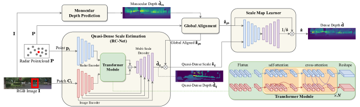
Figure 2: The overall framework of our proposed RadarCam-Depth, comprised with four stages: monocular depth prediction, global alignment of mono-depth with sparse Radar depth, learned quasi-dense scale estimation, and scale map learner for refining local scale of dense depth estimation. $\mathbf{d}$ and $\mathbf{s}$ denotes the depth and scale, while $\mathbf{z}=1/\mathbf{d}$ is the inverse depth.

The primary contributions of this work are as follows: (i) We introduce the first approach that enhances the highly generalizable, scaleless mono-depth prediction with the dense metric scale intricately inferred from the noisy and sparse Radar data. (ii) We present a novel metric dense depth estimation framework that effectively fuses heterogeneous Radar and camera data. Our framework comprises four stages: monocular depth prediction, global scale alignment of the monocular depth, Radar-Camera quasi-dense scale estimation, and scale map learner for refining the quasi-dense scale locally. (iii) The proposed method is extensively tested on the nuScenes benchmark and our self-collected ZJU-4DRadarCam dataset. It outperforms the state-of-the-art (SOTA) techniques, substantially enhancing Radar-Camera dense depth estimation with high metric accuracy and solid generalizability. (iv) To address the absence of a 4D Radar-based depth estimation dataset, we will release our high-quality ZJU-4DRadarCam dataset, including raw 4D Radar data, RGB images, and meticulously generated ground-truth depth maps from LiDAR measurements. Additionally, our code will be open-sourced to fertilize further research.

II RELATED WORK

II-A Monocular Depth Estimation

Monocular depth estimation is a challenging task due to the inherent scale ambiguity. Despite its simplicity and the availability of raw data, researchers have made significant efforts to address this issue by integrating it with optical flow [14], uncertainty estimation [15], semantic segmentation [16], instance segmentation [17] and visual odometry [18]. Although some previous studies [19, 20, 4, 3] have achieved promising results in affine-invariant scaleless depth estimation across diverse datasets, recovering the metric scale still poses a significant challenge. Some existing methods rely on inertial data to provide scale. To enhance the generalization, VI-SLAM [21] warps the input image to match the orientation prevailing in the training dataset. Zuo et al.’s CodeVIO [22] proposes a tightly coupled VIO system with optimizable learned dense depth. It jointly estimates VIO poses and optimizes the predicted and encoded dense depth of certain keyframes efficiently. Similarly, Xie [23] utilizes a flow-to-depth layer to refine camera poses and generate depth proposals. They solve a multi-frame triangulation problem to enhance the estimation accuracy. Recently, Wofk [5] introduced a framework for metric dense depth estimation from the VIO sparse depth and monocular depth prediction, which inspires our work. They first globally align the scaleless mono-depth with the metric VIO sparse depth, and then learn to refine the dense scale of the globally aligned mono-depth.

II-B Depth Estimation from Radar-Camera Fusion

Fusion of Radar and camera data for metric depth estimation is an area of active research. Lin et al. [8] introduced a two-stage CNN-based pipeline that combines Radar and camera inputs to denoise Radar signals and estimate dense depth. Long et al. [9] proposed a Radar-2-Pixel (R2P) network that utilizes radial Doppler velocity and induced optical flow from images to associate Radar points with corresponding pixel regions, enabling the synthesis of full-velocity information. They also achieved image-guided depth completion using Radar and video data [10]. Another approach, DORN [11] proposed by Lo et al, extends Radar points in the elevation dimension and applies deep ordinal regression network-based [24] feature fusion. Unlike other methods, R4dyn [13] creatively incorporates Radar as a weakly supervised signal into a self-supervised framework and employs Radar as an additional input to enhance the robustness. However, their method primarily focuses on vehicle targets and does not fully correlate all Radar points with a larger image area, resulting in lower depth accuracy. However, the above methods require multi-frame information to overcome the sparsity of Radar data. In contrast, Singh et al. [12] presented a fusion method that relies solely on a single image frame and Radar point cloud. Their first-stage network infers the confidence scores of associating a Radar point to image patches, which leads to a semi-dense depth map after association. They further employ a gated fusion network to control the fusion of multi-modal Radar-Camera data, and predict the final dense depth.

III METHODOLOGY

Our goal is to recover the dense depth $\mathbf{\hat{d}}\in\mathbb{R}^{H_{0}\times W_{0}}_{+}$ from a pair of RGB image $\mathbf{I}\in\mathbb{R}^{3\times H_{0}\times W_{0}}$ and Radar point cloud $\mathbf{P}=\left\{\mathbf{p}_{i}|\mathbf{p}_{i}\in\mathbb{R}^{3},i=0,1,2,\cdots,k-1\right\}$ in the image coordinate. Either 3D or 4D Radar usually has a small field of view with ambiguous sparse data deteriorated by intensive noises. To enable the cross-modal fusion, it is straightforward to project Radar points onto the image plane, generating Radar depth. However, direct fusion of the inherently ambiguous and sparse Radar depth with images, achieved by concatenating their encodings or raw data, can confuse the learning pipeline [25, 26, 27, 12], which results in aliasing and other undesirable artifacts in the estimated depth. In this paper, we propose to get the scaleless dense depth with existing versatile monocular depth prediction networks, then learn to augment scaleless dense depth with accurate dense metric scales from Radar data.

The framework of our Radar-Camera depth estimation method consists of four stages: scaless monocular depth prediction, global alignment (GA) of mono-depth, quasi-dense scale estimation, and scale map learner (SML) for refining dense scale locally, as shown in Fig.2.

III-A Monocular Depth Prediction

We employ off-the-shelf networks to predict robust and accurate scaleless depth from a single-view image. The high quality of the mono-depth prediction furnishes a solid foundation for scale-oriented learning. In this research, we harnessed SOTA mono-depth networks, like MiDaS v3.1 [19, 3] and DPT-Hybrid [20] with pre-trained weights on mixed diverse datasets. Both networks are built upon transformer architecture [28] and trained with scale and offset-invariant losses, ensuring strong generalization. They infer the relative depth relationship between pixels, producing dense depth (See Fig.3). Notably, our framework is versatile and compatible with arbitrary mono-depth prediction networks that predict depth $\mathbf{\hat{d}}_{m}$, inverse depth $\mathbf{\hat{z}}_{m}$ or others.

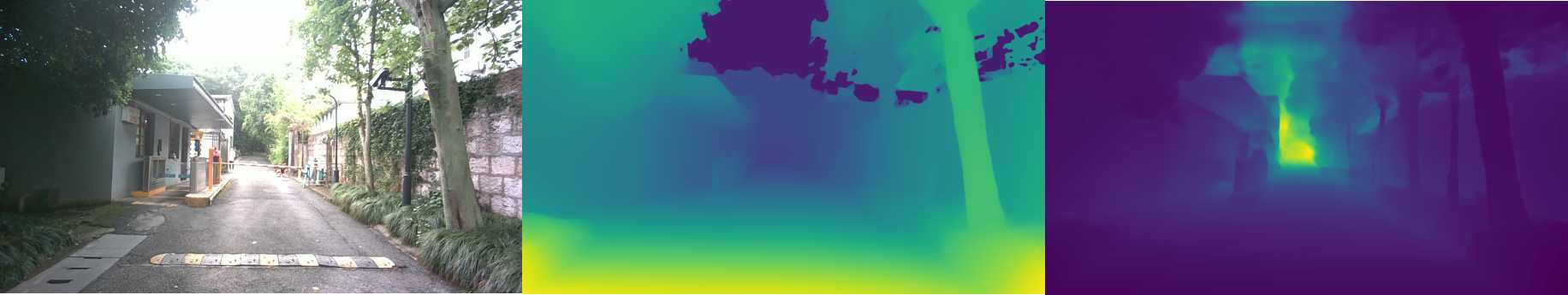
Figure 3: Mono-depth predictions by MiDaS v3.1 [3] and DPT-Hybrid [20]. Notably, MiDaS exhibits the ability to differentiate the sky.

III-B Global Alignment

We align the scaleless monocular depth prediction $\mathbf{\hat{d}}_{m}$ with the Radar depth originating from projecting raw Radar points $\mathbf{P}$, by a global scaling factor $\hat{s}_{g}$ and optional offset $\hat{t}_{g}$. The global aligned metric monocular depth is calculated by $\mathbf{\hat{d}}_{ga}=\hat{s}_{g}\cdot\mathbf{\hat{d}}_{m}+\hat{t}_{g}$. The globally aligned mono-depth is fed into the subsequent scale map learner (SML). There are many options for performing this global alignment between the projected Radar depth and mono-depth prediction, including: (i) Var: A varying $\hat{s}_{g}$ for individual frame of mono-depth, calculated via root-finding algorithms [29, 30]. (ii) Const: A constant $\hat{s}_{g}$ for all frames of mono-depth prediction, deemed as the mean of scale estimates on the entire training samples. (iii) LS: $\hat{s}_{g}$ and $\hat{t}_{g}$ for individual frames, computed with linear least-squares optimization [19]. (iv) RANSAC: $\hat{s}_{g}$ and $\hat{t}_{g}$ for individual frames, computed with linear least-squares while incorporating RANSAC outlier rejection of the Radar depth. We randomly sample 5 Radar points with valid values, estimate $\hat{s}_{g}$ and $\hat{t}_{g}$ with the sampled Radar depth, and adopt the first pair of $\hat{s}_{g}$ and $\hat{t}_{g}$ that yields an inlier ratio over $90\%$. Suppose the discrepancy between Radar depth and aligned mono-depth at the corresponding pixel location is under $6$m (or the inverse depth discrepancy is under $0.015$). In that case, it is a pair of inlier associations.

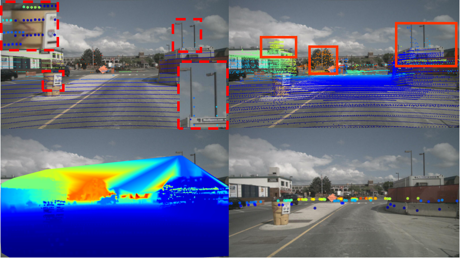
(a)

(b)

Figure 4: (a) Top: nuScenes dataset [31] with LiDAR depth $\mathbf{d}_{gt}$ and accumulated LiDAR depth $\mathbf{d}_{acc}$, depth from 3D Radar point cloud $\mathbf{P}$, interpolated LiDAR $\mathbf{d}_{int}$ shown clockwise. The misalignment between LiDAR points and image pixels on this dataset is highlighted with red boxes. Depth from 3D Radar point cloud is very sparse and non-uniformly distributed. (b) Our ZJU-4DRadarCam dataset with LiDAR depth $\mathbf{d}_{gt}$, interpolated LiDAR depth $\mathbf{d}_{int}$, and depth from 4D Radar point cloud $\mathbf{P}$ shown from top to bottom. Compared to nuScenes, ZJU-4DRadarCam dataset offers more accurate and denser LiDAR depth, as well as denser 4D Radar depth.

III-C Quasi-Dense Scale Estimation

Due to inherent sparsity and noises in Radar data, additional enhancement of raw Radar depth is crucial before conducting the scale map learner. To densify the sparse Radar depth obtained from projection, we exploit a transformer-based Radar-Camera data association network (shorthand RC-Net), which predicts the confidence of Radar-Pixel associations. Pixels without a direct correspondence of Radar point during projection might be associated with the depth of neighboring Radar point, thereby densifying the sparse Radar depth to a quasi-dense depth map, denoted as $\mathbf{\hat{d}}_{q}$.

III-C1 Network Architecture

Our RC-Net (see Fig. 2) is adapted from existing vanilla network RC-vNet [12] by further incorporating self and cross-attention [32] in a transformer module. The image encoder is a standard ResNet18 backbone [33] with 32, 64, 128, 128, 128 channels in each layer, and the Radar encoder is a multi-layer perceptron consisting of fully connected layers with 32, 64, 128, 128, 128 channels. The Radar features are mean pooled and reshaped to the shape of image features. Subsequently, Radar and image features are flattened and passed through $N=4$ layers of self and cross-attention, which involves a larger receptive field for the cross-modal association. These features, combined with skip connections from intermediate layers in the encoder, are forwarded to a decoder with logit output. Finally, the logits are activated by the sigmoid function to obtain the confidence map of cross-modal associations.

III-C2 Confidence of Cross-Modal Associations

For a Radar point $\mathbf{p}_{i}$ and a cropped image patch $\mathbf{C}_{i}\in\mathbb{R}^{3\times H\times W}$ in its projection vicinity, we use RC-Net $h_{\theta}$ to obtain a confidence map $\mathbf{\hat{y}}_{i}=h_{\theta}(\mathbf{C}_{i},\mathbf{p}_{i})\in[0,1]^{H\times W}$, which describes probability of whether the pixels in $\mathbf{C}_{i}$ corresponds to $\mathbf{p}_{i}$. With $k$ points in a Radar point cloud $\mathbf{P}$, the forward pass generates $k$ confidence maps for individual Radar points. Therefore, each pixel $\mathbf{x}_{uv}$, $(u\in[0,W_{0}-1],v\in[0,H_{0}-1])$ within image $\mathbf{I}$ has $n\in[0,k]$ associated Radar point candidates. By selecting the maximum score above the threshold $\tau$, we can find the corresponding Radar point $\mathbf{p}_{\mu}$ for pixel $\mathbf{x}_{uv}$, and assign the depth of $\mathbf{p}_{\mu}$ to $\mathbf{x}_{uv}$. Ultimately, this stage yields a quasi-dense depth map $\mathbf{\hat{d}}_{q}\in\mathbb{R}^{H_{0}\times W_{0}}_{+}$:

$$\hat{\mathbf{d}}_{q}(u,v)=\begin{cases}d(p_{\mu}),\ \ \ \ \text{if}\ \mathbf{\hat{y}}_{\mu}(x_{uv})>\ \tau\\ \text{None},\ \ \ \ \ \text{otherwise}\end{cases}$$ (1)

where $\mu=\underset{i}{\arg\max}\ \mathbf{\hat{y}}_{i}(x_{uv})$, $\mathbf{p}_{\mu}$ is the Radar point has the highest confidence score with $\mathbf{x}_{uv}$, $d(\cdot)$ returns the depth value. Finally, quasi-dense scale map $\mathbf{\hat{s}}_{q}$ is calculated from $\mathbf{\hat{s}}_{q}=\mathbf{\hat{d}}_{q}/\mathbf{\hat{d}}_{ga}$, and its inverse $1/\mathbf{\hat{s}}_{q}$ is subsequently fed into the scale map learner.

III-C3 Training

For the nuScenes dataset, we first project multiple frames to the current LiDAR frame $\mathbf{d}_{gt}$ to obtain the cumulative $\mathbf{d}_{acc}$. After that, linear interpolation in log space [34] is performed on $\mathbf{d}_{acc}$ to obtain $\mathbf{d}_{int}$. Because of its density, $\mathbf{d}_{gt}$ is directly interpolated without accumulation for the ZJU-4DRadarCam dataset. For supervision, we use $\mathbf{d}_{int}$ to build binary classification labels $\mathbf{y}_{i}\in\left\{0,1\right\}^{H\times W}$, where points with a depth difference less than 0.5m from the Radar point are labeled as positive. After constructing $\mathbf{y}_{i}$, we minimize the binary cross-entropy loss:

$$\begin{split}\mathcal{L}_{BCE}=\frac{1}{|\Omega|}\sum_{x\in\Omega}-(\mathbf{y}_{i}(x)\log\mathbf{\hat{y}}_{i}(x)\\ +(1-\mathbf{y}_{i}(x))\log(1-\mathbf{\hat{y}}_{i}(x)))\end{split}$$ (2)

where $\Omega\subset\mathbb{R}^{2}$ denotes the spatial image domain of $\mathbf{C}_{i}$, $x\in\Omega$ is a pixel coordinate, and $\mathbf{\hat{y}}_{i}=h_{\theta}(\mathbf{C}_{i},\mathbf{p}_{i})$ is the confidence of correspondence.

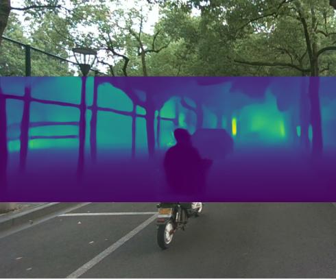
(a)

(b)

Figure 5: (a) Our metric depth estimation over the input image in a cluttered large-scale scenario. (b) Top row shows the ground truth depth $\mathbf{d}_{int}$ and Radar points $\mathbf{P}$ projected into image $\mathbf{I}$. The rest rows from top to bottom depict the depth estimations of [11], [12], and our RadarCam-Depth and the corresponding error maps. Our method demonstrates much higher accuracy and fine details.

III-D Scale Map Learner

III-D1 Network Architecture

Inspired by [5], we construct a scale map learner (SML) network based on MiDaS-small [19] architecture. SML aims to learn a pixel-level dense scaling map for $\mathbf{\hat{d}}_{ga}$, which completes the quasi-dense scale map and refine the metric accuracy of $\mathbf{\hat{d}}_{ga}$. SML requires concatenated $\mathbf{\hat{z}}_{ga}$ and $1/\mathbf{\hat{s}}_{q}$ as input. The empty locations in $\mathbf{\hat{s}}_{q}$ are filled with ones. SML regresses a dense scale residual map $\mathbf{r}$, where values can be negative. We obtain the final scale map via $1/\mathbf{\hat{s}}=\text{ReLU}(1+\mathbf{r})$, and the final metric depth estimation is computed by $\mathbf{\hat{d}}=\mathbf{\hat{s}}/\mathbf{\hat{z}}_{ga}$.

III-D2 Training

Ground truth depth $\mathbf{d}_{gt}$ is obtained from projecting 3D LiDAR points. LiDAR depth is further interpolated to get a densified depth $\mathbf{d}_{int}$. During training, we minimize the difference between the estimated metric dense depth $\hat{\mathbf{d}}$ and $\mathbf{d}_{gt}$/$\mathbf{d}_{int}$ with a smoothed L1 penalty:

$$\mathcal{L}_{SML}=\mathcal{L}(\mathbf{d}_{int},\hat{\mathbf{d}})+\lambda_{gt}\mathcal{L}(\mathbf{d}_{gt},\hat{\mathbf{d}})$$ (3)

$$\mathcal{L}(\mathbf{d},\hat{\mathbf{d}})=\begin{cases}\frac{1}{|\Omega_{d}|}\underset{x\in\Omega_{d}}{\sum}(\mathbf{r}_{d}(x)-\beta/2),\ \text{if}\ \mathbf{r}_{d}(x)<\beta\\ \frac{1}{|\Omega_{d}|}\underset{x\in\Omega_{d}}{\sum}(\mathbf{r}_{d}(x)^{2}/2\beta),\ \ \ \text{otherwise}\end{cases}$$ (4)

where $\mathbf{r}_{d}(x)=|\mathbf{d}(x)-\hat{\mathbf{d}}(x)|$, $\lambda_{gt}$ is the weight of $\mathcal{L}_{gt}$, $\Omega_{d}\subset\Omega$ denotes the domains where ground truth has valid depth values. $\beta$ is set to 1 in our practice.

IV EXPERIMENTS

IV-A Datasets

We first evaluate the proposed method on nuScenes benchmark [31]. NuScenes dataset encompasses data collection across 1000 scenes in Boston and Singapore with LiDAR, 3D Radar, camera, and IMU sensors. It comprises around 40000 synchronized Radar-Camera keyframes. We followed the same data splits as [12] with 850 scenes for training and validation and 150 for testing. The test split is officially offered by nuScenes v1.0.

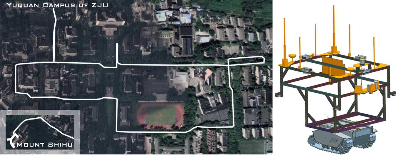
Figure 6: Our data collection routes and the CAD model of our ground robot.

For extensive evaluation, we collected our own dataset, named ZJU-4DRadarCam, using a ground robot (Fig.6) equipped with Oculii’s EAGLE 4D Radar, RealSense D455 camera, and RoboSense M1 LiDAR sensors. Our dataset includes various driving scenarios including urban and wilderness environments. Compared to nuScenes dataset, our ZJU-4DRadarCam offers 4D Radar data with denser measurements, besides, we provide denser LiDAR depth for supervision and evaluation (see Fig.4). Our ZJU-4DRadarCam comprises a total of 33,409 synchronized Radar-Camera keyframes, split into 29312 frames for training and validation, and 4097 frames for testing.

IV-B Training Details and Evaluation Protocol

For the nuScenes dataset, following [12], we accumulate the individual $\mathbf{d}_{gt}$ of 160 frames nearby to get $\mathbf{d}_{acc}$, which is then interpolated to yield $\mathbf{d}_{int}$. Dynamic objects are masked out during the above process. For the ZJU-4DRadarCam dataset, we directly interpolate $\mathbf{d}_{gt}$ to obtain $\mathbf{d}_{int}$ with linear interpolation [34] in the log space of depth.

When training the RC-Net for quasi-dense scale estimation, we utilize the network architecture of [12] with our transformer module. For the training on nuScenes, with an input image size of $900\times 1600$, the size of the cropped patch during confidence map formation is set to $900\times 288$. For the training on ZJU-4DRadarCam, the input image size is $300\times 1280$, while the patch size is $300\times 100$. We employ the Adam optimizer with $\beta_{1}$=0.9 and $\beta_{2}$=0.999, and a learning rate of $2e^{-4}$ for 50 epochs. Data augmentations, including horizontal flipping, saturation, brightness, and contrast adjustments, are applied with a 0.5 probability. We train our RC-Net for 50 epochs with an NVIDIA RTX 3090 GPU, taking approximately 14 hours with a batch size of 6.

We adopt MiDaS-Small architecture in our SML, where the encoder backbone is initialized with pre-trained ImageNet weights [35], and other layers are randomly initialized. The input data is resized and cropped to $288\times 384$. We use an Adam optimizer with $\beta_{1}=0.9$ and $\beta_{2}=0.999$. The initial learning rate is set to $2e^{-4}$ and reduced to $5e^{-5}$ after 20 epochs. Training SML for 40 epochs takes about 24 hours with a batch size of 24.

Some widely adopted metrics from the literature are used for evaluating the depth estimations, including mean absolute error (MAE), root mean squared error (RMSE), absolute relative error (AbsRel), squared relative error (SqRel), the errors of inverse depth (iRMSE, iMAE), and $\delta_{1}$ [36].

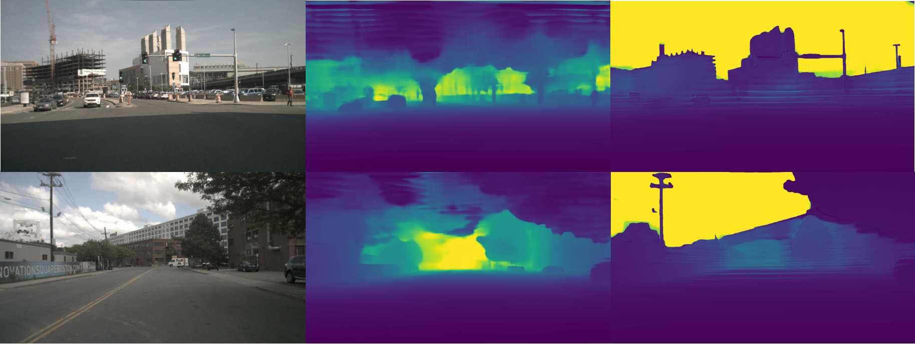
Figure 7: From left to right are the input images, depth estimaiton of [12], and depth estimation of our RadarCam-Depth on nuScenes benchmark. Ours accurately differentiates the sky region and preserves fine details on object boundaries.

IV-C Evaluation on NuScenes

We evaluate the metric dense depth against $\mathbf{d}_{gt}$ within the range of 50, 70, and 80 meters (see Tab.I). Our proposed RadarCam-Depth outperforms all the compared Radar-Camera methods and surpasses the second best method [12] by a large margin at all ranges. Specifically, we observe 25.6%, 23.4%, and 22.5% reductions in MAE and 20.9%, 20.2%, and 19.4% drops in RMSE for 50m, 70m, and 80m, respectively. Furthermore, our approach obviates the need to aggregate multi-frame Radar point clouds or multi-view images. Our method solely relies on a single-frame image and a Radar point cloud, thus enhancing its real-time capabilities. The ”Radar” and ”Image” columns in Tab.I specify the quantities of Radar point clouds and images used as inputs in various methods.

The images in nuScenes contain large regions corresponding to the sky. For our framework’s monocular depth prediction network, we adopt the sky-sensitive pre-trained model, MiDaS v3.1, which can accurately differentiate the sky from others (see Fig.3). However, since the depth estimations in sky regions are not associated with corresponding LiDAR depth, they are not counted during metric evaluations. Some snapshots of depth estimations from different methods are shown in Fig.7.

TABLE I: Evaluations on NuScenes (mm)

Eval Dist	Method	Radar	Image	MAE	RMSE
50m	RC-PDA [10]	5	3	2225.0	4156.5
	RC-PDA with HG [10]	5	3	2315.7	4321.6
	DORN [11]	5(x3)	1	1926.6	4124.8
	Singh [12]	1	1	1727.7	3746.8
	RadarCam-Depth	1	1	1286.1	2964.3
70m	RC-PDA [10]	5	3	3326.1	6700.6
	RC-PDA with HG [10]	5	3	3485.6	7002.9
	DORN [11]	5(x3)	1	2380.6	5252.7
	Singh [12]	1	1	2073.2	4590.7
	RadarCam-Depth	1	1	1587.9	3662.5
80m	RC-PDA [10]	5	3	3713.6	7692.8
	RC-PDA with HG [10]	5	3	3884.3	8008.6
	DORN [11]	5(x3)	1	2467.7	5554.3
	Lin [8]	3	1	2371.0	5623.0
	R4Dyn [13]	4	1	N/A	6434.0
	Sparse-to-dense [37]	3	1	2374.0	5628.0
	PnP [38]	3	1	2496.0	5578.0
	Singh [12]	1	1	2179.3	4898.7
	RadarCam-Depth	1	1	1689.7	3948.0

IV-D Evaluation on ZJU-4DRadarCam

We follow a similar way to Sec.IV-C for the evaluations on the ZJU-4DRadarCam dataset. For the mono-depth prediction in our framework, we tried both MiDaS v3.1 [3] and DPT-Hybrid [20] models. The evaluations of the metric dense depth estimations from various methods are presented in Tab.II, where our approach at different configurations of mono-depth network and global alignment options are marked in bold. After a comprehensive evaluation, we observe that our methods with the DPT model performs better for depth metrics, while the methods with MiDaS demonstrates higher accuracy for inverse depth metrics. Overall, our proposed methodology exhibits significant improvements compared to existing Radar-Camera methods [12] and [11] (Fig.5(b)). Compared to the second best [12], the best configuration of our method shows 40.2%, 40.1%, and 40.2% reductions in MAE, and 24.3%, 24.6%, and 25.1% drops in RMSE within ranges of 50m, 70m, and 80m, respectively.

TABLE II: Evaluations on ZJU-4DRadarCam (mm)

Dist	Method	MAE	RMSE	iMAE	iRMSE	AbsRel	SqRel	$\mathbf{\delta_{1}}$
50m	DORN [11]	2210.171	4129.691	19.790	31.853	0.157	939.348	0.783
	Singh [12]	1785.391	3704.636	18.102	35.342	0.146	966.133	0.831
	DPT+Var+RC-vNet [12]	1243.339	3045.853	12.111	24.377	0.098	644.709	0.896
	DPT+Const+RC-Net	1082.927	2803.180	10.885	23.227	0.089	561.834	0.920
	DPT+Var+RC-Net	1067.531	2817.362	10.508	22.936	0.087	575.838	0.922
	MiDaS+Var+RC-Net	1177.257	3009.135	10.255	22.385	0.090	630.222	0.924
	MiDaS+LS+RC-Net	1083.691	2868.950	10.059	22.388	0.086	588.091	0.928
70m	DORN [11]	2402.180	4625.231	19.848	31.877	0.160	1021.805	0.777
	Singh [12]	1932.690	4137.143	17.991	35.166	0.147	1014.454	0.828
	DPT+Var+RC-vNet [12]	1337.649	3358.212	12.047	24.294	0.099	672.084	0.894
	DPT+Const+RC-Net	1178.046	3121.317	10.824	23.149	0.090	589.377	0.918
	DPT+Var+RC-Net	1157.014	3117.721	10.444	22.853	0.087	601.052	0.921
	MiDaS+Var+RC-Net	1280.124	3323.488	10.189	22.300	0.091	658.416	0.922
	MiDaS+LS+RC-Net	1177.253	3179.615	9.996	22.305	0.086	614.801	0.926
80m	DORN [11]	2447.571	4760.016	19.856	31.879	0.161	1038.919	0.776
	Singh [12]	1979.459	4309.314	17.971	35.133	0.147	1034.148	0.828
	DPT+Var+RC-vNet [12]	1365.383	3467.245	12.033	24.277	0.099	682.126	0.894
	DPT+Const+RC-Net	1206.541	3239.331	10.812	23.133	0.090	599.674	0.918
	DPT+Var+RC-Net	1183.471	3228.999	10.432	22.838	0.088	610.501	0.920
	MiDaS+Var+RC-Net	1309.859	3431.046	10.176	22.282	0.091	668.038	0.922
	MiDaS+LS+RC-Net	1205.137	3295.520	9.984	22.289	0.086	624.864	0.926

We report our proposed method’s runtime at the DPT-based mono-depth prediction configuration. The average processing times per frame are shown in Tab.III. Note that Mono-Pred and GA can run simultaneously with RC-Net. Regarding different scale global alignment methods, GA (Var) and GA (LS) exhibit relatively fast speeds, while GA (RANSAC) is significantly slow and not advocated.

TABLE III: Runtime (s)

Mono-Pred	GA (Const)	GA (Var)	GA (LS)	GA (RANSAC)	RC-Net	SML
0.0651	-	0.0624	0.0044	2.2903	0.2704	0.1227

IV-E Ablation

IV-E1 Transformer Module

We commence our analysis by focusing on the transformer mechanism incorporated within our novel quasi-dense scale estimation module, RC-Net. When the transformer component is disengaged, the architecture is identical to the pre-existing vanilla network, RC-vNet [12]. Our evaluation is conducted on the ZJU-4DRadarCam datasets, and the results are presented in Tab.IV. The comparison results are the error in quasi-dense depth estimation $\mathbf{\hat{d}}_{q}$ against ground truth $\mathbf{d}_{gt}$ within a range of 80 meters. Our RC-Net consistently outperforms RC-vNet across all evaluation metrics, as delineated in Tab.IV. Furthermore, as also indicated in Tab.II, when integrated with the DPT+Var framework, DPT+Var+RC-Net exhibits notable performance superiority over its RC-vNet counterpart.

TABLE IV: Ablation of Transformer Module (mm)

Dataset	Method	MAE	RMSE	iMAE	iRMSE	Output Pts
ZJU-4D	RC-vNet [12]	1308.742	3339.697	20.418	38.540	172567.846
	RC-Net	1083.305	3052.870	16.203	33.414	178713.881

IV-E2 Global Alignment

Following the discussions in Sec.III-B, we systematically assess the four options for globally aligning the scale of mono-depth predictions. It is worth mentioning that we set a termination criterion of 400 iterations for the GA (RANSAC), at which point we halt the iterative process and select the values of $\hat{s}_{g}$ and $\hat{t}_{g}$ that yield the highest inlier ratio. The evaluation results of $\hat{\mathbf{d}}_{ga}$ are presented in Tab.V within a range of 80 m. Combining the runtime performance in III, the best GA method for ZJU-4D (DPT) is aligning with variable $\hat{s}_{g}$ (Var), and the optimal method for ZJU-4D (MiDaS) is least-squares for $\hat{s}_{g}$ and $\hat{t}_{g}$ (LS). The experiments showcase that estimating $\hat{t}_{g}$ for DPT leads to substantial inverse errors, significantly degrading the performance of the subsequent SML (conducted in inverse space). However, ZJU-4D (MiDaS) require simultaneous estimating $\hat{s}_{g}$ and $\hat{t}_{g}$ to achieve higher accuracy.

TABLE V: Ablation of GA Module (mm)

Data	Method	MAE	RMSE	iMAE	iRMSE	AbsRel	SqRel	$\mathbf{\delta_{1}}$
ZJU-4D (DPT)	Const	4733.158	6926.261	37.942	53.913	0.392	2501.383	0.343
	Var	4726.168	6940.025	36.531	52.569	0.386	2569.835	0.374
	LS	5671.214	7409.278	111.292	530.436	0.552	4069.064	0.271
	RANSAC	5963.904	7662.980	336.568	1294.117	0.614	4732.633	0.277
ZJU-4D (MiDaS)	Const	14008.482	245011.138	38.973	51.691	0.752	25697452.430	0.358
	Var	7119.828	14297.549	32.285	46.340	0.468	13255.805	0.431
	LS	4799.150	7968.478	35.670	51.559	0.390	4659.651	0.394
	RANSAC	5113.080	11063.605	23.920	37.881	0.347	13322.258	0.631

V Conclusion

This paper presents a novel method for estimating dense metric depth by integrating monocular depth prediction with the scale from sparse and noisy Radar point cloud. We propose a dedicated four-stage framework that effectively combines the high-fidelity fine details of the image and the absolute scale of Radar data, surmounting the inherent challenges of detail loss and the imprecision of metrics that manifest in existing methods based on the direction fusion of Radar and image data or their encodings. Our experimental findings unequivocally demonstrate a significantly superior performance of the proposed methodology over the compared baseline, as substantiated by both quantitative and qualitative assessments. In general, we introduce a pioneering metric depth estimation solution, which is rigorously validated and suitable for application on fusing cameras with 3D or 4D Radars.

References

- [1] Zachary Teed and Jia Deng “Deepv2d: Video to depth with differentiable structure from motion” In arXiv preprint arXiv:1812.04605, 2018
- [2] Alex Wong, Xiaohan Fei, Stephanie Tsuei and Stefano Soatto “Unsupervised depth completion from visual inertial odometry” In IEEE Robotics and Automation Letters 5.2 IEEE, 2020, pp. 1899–1906
- [3] Reiner Birkl, Diana Wofk and Matthias Müller “MiDaS v3.1 – A Model Zoo for Robust Monocular Relative Depth Estimation” In arXiv preprint arXiv:2307.14460, 2023
- [4] Vitor Guizilini, Igor Vasiljevic, Dian Chen, Rares Ambrus and Adrien Gaidon “Towards Zero-Shot Scale-Aware Monocular Depth Estimation” In arXiv preprint arXiv:2306.17253, 2023
- [5] Diana Wofk, René Ranftl, Matthias Müller and Vladlen Koltun “Monocular Visual-Inertial Depth Estimation” In arXiv preprint arXiv:2303.12134, 2023
- [6] Yukai Ma, Xiangrui Zhao, Han Li, Yaqing Gu, Xiaolei Lang and Yong Liu “RoLM: Radar on LiDAR Map Localization” In 2023 IEEE International Conference on Robotics and Automation (ICRA), 2023, pp. 3976–3982 IEEE
- [7] Yukai Ma, Han Li, Xiangrui Zhao, Yaqing Gu, Xiaolei Lang, Laijian Li and Yong Liu “FMCW Radar on LiDAR Map Localization in Structual Urban Environments”, 2023
- [8] Juan-Ting Lin, Dengxin Dai and Luc Van Gool “Depth estimation from monocular images and sparse radar data” In 2020 IEEE/RSJ International Conference on Intelligent Robots and Systems (IROS), 2020, pp. 10233–10240 IEEE
- [9] Yunfei Long, Daniel Morris, Xiaoming Liu, Marcos Castro, Punarjay Chakravarty and Praveen Narayanan “Full-velocity radar returns by radar-camera fusion” In Proceedings of the IEEE/CVF International Conference on Computer Vision, 2021, pp. 16198–16207
- [10] Yunfei Long, Daniel Morris, Xiaoming Liu, Marcos Castro, Punarjay Chakravarty and Praveen Narayanan “Radar-camera pixel depth association for depth completion” In Proceedings of the IEEE/CVF Conference on Computer Vision and Pattern Recognition, 2021, pp. 12507–12516
- [11] Chen-Chou Lo and Patrick Vandewalle “Depth estimation from monocular images and sparse radar using deep ordinal regression network” In 2021 IEEE International Conference on Image Processing (ICIP), 2021, pp. 3343–3347 IEEE
- [12] Akash Deep Singh, Yunhao Ba, Ankur Sarker, Howard Zhang, Achuta Kadambi, Stefano Soatto, Mani Srivastava and Alex Wong “Depth Estimation From Camera Image and mmWave Radar Point Cloud” In Proceedings of the IEEE/CVF Conference on Computer Vision and Pattern Recognition, 2023, pp. 9275–9285
- [13] Stefano Gasperini, Patrick Koch, Vinzenz Dallabetta, Nassir Navab, Benjamin Busam and Federico Tombari “R4Dyn: Exploring radar for self-supervised monocular depth estimation of dynamic scenes” In 2021 International Conference on 3D Vision (3DV), 2021, pp. 751–760 IEEE
- [14] Wang Zhao, Shaohui Liu, Yezhi Shu and Yong-Jin Liu “Towards better generalization: Joint depth-pose learning without posenet” In Proceedings of the IEEE/CVF Conference on Computer Vision and Pattern Recognition, 2020, pp. 9151–9161
- [15] Matteo Poggi, Filippo Aleotti, Fabio Tosi and Stefano Mattoccia “On the uncertainty of self-supervised monocular depth estimation” In Proceedings of the IEEE/CVF Conference on Computer Vision and Pattern Recognition, 2020, pp. 3227–3237
- [16] Lukas Hoyer, Dengxin Dai, Qin Wang, Yuhua Chen and Luc Van Gool “Improving semi-supervised and domain-adaptive semantic segmentation with self-supervised depth estimation” In International Journal of Computer Vision Springer, 2023, pp. 1–27
- [17] Jiawang Bian, Zhichao Li, Naiyan Wang, Huangying Zhan, Chunhua Shen, Ming-Ming Cheng and Ian Reid “Unsupervised scale-consistent depth and ego-motion learning from monocular video” In Advances in neural information processing systems 32, 2019
- [18] Xiaogang Song, Haoyue Hu, Li Liang, Weiwei Shi, Guo Xie, Xiaofeng Lu and Xinhong Hei “Unsupervised Monocular Estimation of Depth and Visual Odometry uUsing Attention and Depth-Pose Consistency Loss” In IEEE Transactions on Multimedia IEEE, 2023
- [19] René Ranftl, Katrin Lasinger, David Hafner, Konrad Schindler and Vladlen Koltun “Towards robust monocular depth estimation: Mixing datasets for zero-shot cross-dataset transfer” In IEEE transactions on pattern analysis and machine intelligence 44.3 IEEE, 2020, pp. 1623–1637
- [20] René Ranftl, Alexey Bochkovskiy and Vladlen Koltun “Vision transformers for dense prediction” In Proceedings of the IEEE/CVF international conference on computer vision, 2021, pp. 12179–12188
- [21] Kourosh Sartipi, Tien Do, Tong Ke, Khiem Vuong and Stergios I Roumeliotis “Deep depth estimation from visual-inertial slam” In 2020 IEEE/RSJ International Conference on Intelligent Robots and Systems (IROS), 2020, pp. 10038–10045 IEEE
- [22] Xingxing Zuo, Nathaniel Merrill, Wei Li, Yong Liu, Marc Pollefeys and Guoquan Huang “CodeVIO: Visual-inertial odometry with learned optimizable dense depth” In 2021 ieee international conference on robotics and automation (icra), 2021, pp. 14382–14388 IEEE
- [23] Jiaxin Xie, Chenyang Lei, Zhuwen Li, Li Erran Li and Qifeng Chen “Video depth estimation by fusing flow-to-depth proposals” In 2020 IEEE/RSJ International Conference on Intelligent Robots and Systems (IROS), 2020, pp. 10100–10107 IEEE
- [24] Huan Fu, Mingming Gong, Chaohui Wang, Kayhan Batmanghelich and Dacheng Tao “Deep ordinal regression network for monocular depth estimation” In Proceedings of the IEEE conference on computer vision and pattern recognition, 2018, pp. 2002–2011
- [25] Yanchao Yang, Alex Wong and Stefano Soatto “Dense depth posterior (ddp) from single image and sparse range” In Proceedings of the IEEE/CVF Conference on Computer Vision and Pattern Recognition, 2019, pp. 3353–3362
- [26] Wouter Van Gansbeke, Davy Neven, Bert De Brabandere and Luc Van Gool “Sparse and noisy lidar completion with rgb guidance and uncertainty” In 2019 16th international conference on machine vision applications (MVA), 2019, pp. 1–6 IEEE
- [27] Alex Wong and Stefano Soatto “Unsupervised depth completion with calibrated backprojection layers” In Proceedings of the IEEE/CVF International Conference on Computer Vision, 2021, pp. 12747–12756
- [28] Alexey Dosovitskiy, Lucas Beyer, Alexander Kolesnikov, Dirk Weissenborn, Xiaohua Zhai, Thomas Unterthiner, Mostafa Dehghani, Matthias Minderer, Georg Heigold and Sylvain Gelly “An image is worth 16x16 words: Transformers for image recognition at scale” In arXiv preprint arXiv:2010.11929, 2020
- [29] George E Forsythe “Computer methods for mathematical computations” Prentice-hall, 1977
- [30] Richard P Brent “Algorithms for minimization without derivatives” Courier Corporation, 2013
- [31] Holger Caesar, Varun Bankiti, Alex H Lang, Sourabh Vora, Venice Erin Liong, Qiang Xu, Anush Krishnan, Yu Pan, Giancarlo Baldan and Oscar Beijbom “nuscenes: A multimodal dataset for autonomous driving” In Proceedings of the IEEE/CVF conference on computer vision and pattern recognition, 2020, pp. 11621–11631
- [32] Jiaming Sun, Zehong Shen, Yuang Wang, Hujun Bao and Xiaowei Zhou “LoFTR: Detector-free local feature matching with transformers” In Proceedings of the IEEE/CVF conference on computer vision and pattern recognition, 2021, pp. 8922–8931
- [33] Kaiming He, Xiangyu Zhang, Shaoqing Ren and Jian Sun “Deep residual learning for image recognition” In Proceedings of the IEEE conference on computer vision and pattern recognition, 2016, pp. 770–778
- [34] C Bradford Barber, David P Dobkin and Hannu Huhdanpaa “The quickhull algorithm for convex hulls” In ACM Transactions on Mathematical Software (TOMS) 22.4 Acm New York, NY, USA, 1996, pp. 469–483
- [35] Jia Deng, Wei Dong, Richard Socher, Li-Jia Li, Kai Li and Li Fei-Fei “Imagenet: A large-scale hierarchical image database” In 2009 IEEE conference on computer vision and pattern recognition, 2009, pp. 248–255 Ieee
- [36] Jiaming Sun, Yiming Xie, Linghao Chen, Xiaowei Zhou and Hujun Bao “NeuralRecon: Real-time coherent 3D reconstruction from monocular video” In Proceedings of the IEEE/CVF Conference on Computer Vision and Pattern Recognition, 2021, pp. 15598–15607
- [37] Fangchang Ma and Sertac Karaman “Sparse-to-dense: Depth prediction from sparse depth samples and a single image” In 2018 IEEE international conference on robotics and automation (ICRA), 2018, pp. 4796–4803 IEEE
- [38] Tsun-Hsuan Wang, Fu-En Wang, Juan-Ting Lin, Yi-Hsuan Tsai, Wei-Chen Chiu and Min Sun “Plug-and-play: Improve depth estimation via sparse data propagation” In arXiv preprint arXiv:1812.08350, 2018