Predicting the structure of dynamic graphs

Abstract

Dynamic graph embeddings, inductive and incremental learning facilitate predictive tasks such as node classification and link prediction. However, predicting the structure of a graph at a future time step from a time series of graphs, allowing for new nodes has not gained much attention. In this paper, we present such an approach. We use time series methods to predict the node degree at future time points and combine it with flux balance analysis – a linear programming method used in biochemistry – to obtain the structure of future graphs. Furthermore, we explore the predictive graph distribution for different parameter values. We evaluate this method using synthetic and real datasets and demonstrate its utility and applicability.

1 Introduction

Networks are everywhere; from protein-protein interaction networks in biology to social networks on social media platforms, we are surrounded by networks in different mediums and scales. As such, there is a extensive body of research on different aspects of networks/graphs, their embeddings and prediction. Our focus is on predicting the structure of a dynamic, undirected, unweighted network/graph at a future time step including new nodes and edges.

Dynamic graphs such as those encountered in social networks change over time with the addition and deletion of new nodes and edges. In contrast, the structure of static graphs remain constant. For example, while the traffic changes over time in road networks, the underlying graph structure remains the same. Even though static graphs have been studied for longer, there is a lot of interest on dynamic graphs (Pareja et al., 2020; Trivedi et al., 2019; You et al., 2022; Barros et al., 2021; Sankar et al., 2020). The broad applicability of dynamic graphs to many scenarios including recommender systems, autonomous vehicles and social networks make it an expanding research field.

Generally dynamic graphs are represented in two different formats: discrete-time dynamic graphs (DTDG) and continuous-time dynamic graphs (CTDG) (Kazemi et al., 2020). Discrete-time dynamic graphs consider a sequence of graphs at regular time intervals, for example, graphs on social network daily activity. Continuous-time dynamic graphs (CTDG) are more event-driven, where each event can be the formation of an edge, addition of a new node or a similar activity. We focus on discrete-time dynamic graphs (DTDG) in this work.

One of the most popular tasks considered in dynamic graphs is node classification. Predicting the paper subject categories or classifying protein roles in a protein-protein interaction network are node classification examples. Other tasks include graph classification, link prediction, edge classification, entity/relation prediction, time prediction and network clustering. Most tasks consider a sequence of graphs for $i\in\{1,\ldots,t\}$ and predict the required property of the graph at $t+1$ using some information about the graph at $t+1$. For node classification, input features of nodes at time $t+1$ are generally considered when predicting the category of the nodes (Pareja et al., 2020). Link prediction considers if a link exists between two nodes $u$ and $v$. Thus, the nodes at time $t+1$ are known. Dynamic entity/relation prediction predicts a missing entry in the tuple $(u,r,v)$ , where $u$ and $v$ are nodes and $r$ is the relation (Kazemi et al., 2020). In all these scenarios, some information about the graph at time $t+1$ is known. Our work is different from these tasks because we do not know anything about the graph at time $t+1$. From a sequence of graphs, we predict the structure – nodes and edges – of the graph at a future time step. To the best of our knowledge, this task has not been studied before. In this study we consider simple graphs, i.e., unweighted, undirected graphs without any node or edge attributes.

The methods we use are motivated from Flux Balance Analysis (FBA) (Orth et al., 2010) and combined with time series prediction. FBA is a mathematical approach widely used in biochemistry to reconstruct metabolic networks by using linear and mixed-integer programming. By solving an optimization problem maximizing the biomass function subject to a large number of constraints, FBA arrives at the flux solution describing a network of chemical reactions. We adapt FBA to a graph/network prediction framework by considering the degree of each node instead of the flux of chemical reactions. To predict the graph at a future time step, we incorporate the predicted degree of each node in the constraints. Thus, the adapted FBA solution gives us a graph satisfying the degree constraints at a future time step; it predicts the structure of the future graph.

2 Related Work

2.1 Inductive graph learning

Inductive graph learning focuses on changing graph structure and the ability to generalize to unseen nodes. In an inductive setting, all nodes may not be present at the training stage. This is different to transductive learning, where the graph structure used in training is used for testing. Existing work on transductive graph learning and embedding approaches far exceeds that of inductive learning. Inductive learning is mostly used for node classification (Hamilton et al., 2017; Su et al., 2023; Bai et al., 2019; Rossi et al., 2020; Yang et al., 2016). Yang et al. (2016) explain the difference at an architectural level considering the inputs into account. The transductive formulation takes the input features as well as the graph embedding as inputs to predict the class label. Their proposed inductive algorithm Planetoid-I takes only the input features and defines the embedding as a prametrizatized function of the features, which then is used to predict the class label. Citation networks are a popular application of inductive graph learning, where new paper subject categories are predicted using features but without the knowledge of the new graph. Other applications include similarity ranking and graph visualization (Bai et al., 2019) and within-network link classification and link prediction (Rossi et al., 2020) where a graph with a fraction of missing edges is used.

2.2 Incremental and dynamic graph learning

In dynamic network settings such as social networks, the graphs are large and it is computationally prohibitive to retrain a full model at each time step. Thus, it is important to update the model without retraining it from scratch. Due to the significance of the research problem and its strong pertinence, both incremental and dynamic graph learning have attracted a lot of attention (Kim et al., 2022; Tan et al., 2022; Xu et al., 2020; Yin et al., 2021; Yuan et al., 2021; Zhang et al., 2022; Galke et al., 2021; Wang et al., 2020; Han, Karunasekera & Leckie, 2021).

Both Incremental and dynamic graph learning encompass a set of methods that learn from a sequence of graphs and generalize to unseen graphs. However, the two methodologies focus on different aspects of learning. Incremental graph learning also known as continual or lifelong graph learning focuses on overcoming the catastrophic forgetting problem – the significant decrease of model performance of previous tasks after being trained on new tasks (Xu et al., 2020). Methods employed to combat catastrophic forgetting in incremental graph learning can be categorized into three types; regularization-based methods, memory-replay based methods, and parametric isolation based methods. Each category of methods strive to resolve catastrophic forgetting in different ways, either by penalizing changes to parameter updates, selecting representative data from previous tasks or by introducing new parameters to avoid drastic changes.

Dynamic graph learning has a different emphasis. The focus of dynamic graph learning is to capture the temporal dynamics and keep the graph representations up to date (Zhang et al., 2022; Su et al., 2023). The catastrophic forgetting problem is not the focus of dynamic graph learning. While these two topics have different technical emphasis, both incremental and dynamic graph learning train models to perform similar tasks. Two popular tasks for both scenarios are node classification and graph classification. In both settings new nodes can appear and they can belong to new classes as well as existing classes. Similarly new categories of graphs can appear over time.

2.3 Link prediction in dynamic graphs

Link prediction in graphs has a long history (Getoor et al., 2003). The methods used for link prediction can be broadly categorized into probabilistic, spectral clustering, time series, deep learning including embedding and graph neural networks, matrix factorization and other methods (Divakaran & Mohan, 2020). Recent work includes link prediction using neural ordinary differential equations (Luo et al., 2023; Han, Ding, Ma, Gu & Tresp, 2021).

Most work done on link prediction consider the set of nodes as fixed and known beforehand, while the links are unknown (Chen et al., 2022, 2021; Qu et al., 2020; Ma et al., 2018). In this setting, if a node $v_{i}$ appears at time $t_{j}$ and makes its first link with node $v_{k}$, the modeling paradigm assumes the existence of the node from time $t_{0}<t_{j}$ and treats $v_{i}$ as a silent node that makes its first link at time $t_{j}$. In the other setting the set of nodes is more dynamic and not completely known at the beginning. In this setting, they consider the problem “given these nodes, are there links between them?” and evaluate performance on a hidden set of links (Goyal et al., 2017). Thus, the dynamic link prediction problem predicts the links given the nodes at a specific time.

While link prediction, inductive, incremental and dynamic graph learning are related, our work is different as we predict the graph structure including new nodes and edges at a future time point.

3 Methodology

3.1 Notation

We consider a series of undirected, unweighted, growing graphs $\mathcal{G}_{t}=\left(V_{t},E_{t}\right)$ without loops, where $V_{t}\subseteq V_{t+1}$ (also known as projective (Cai et al., 2016)) for time $t\in\{1,\ldots,T\}$ and focus on predicting $\mathcal{G}_{T+h}=\left(V_{T+h},E_{T+h}\right)$. Let $V_{t}=\{v_{1},\ldots,v_{n_{t}}\}$ denote the set of vertices in graph $\mathcal{G}_{t}$ with $|V_{t}|=n_{t}$. Let $e_{ij,t}$ denote the edge between nodes $i$ and $j$ at time $t$, where $i$ and $j$ can denote new or old vertices. Thus, the set of edges in $\mathcal{G}_{t}$ is $E_{t}=\{e_{ij,t}\}_{i,j\in V_{t}}$. Let $d_{i,t}$ denote the degree of vertex $v_{i}$ in $\mathcal{G}_{t}$, i.e., in a unweighted graph setting $d_{i,t}=\sum_{j}e_{ij,t}$. We denote all predictions by a hat $\hat{}$. For example, the predicted number of vertices at time $T+h$ is denoted by $\hat{n}_{T+h}$.

Our aim is to predict $\mathcal{G}_{T+h}=\left(V_{T+h},E_{T+h}\right)$, i.e., the structure of the graph at $T+h$ including new vertices and new edges. In particular we describe, in some form, the distribution of graphs at $t=T+h$ which can include a variable number of nodes and edges. Our approach to predicting $\mathcal{G}_{T+h}$ comprises two steps: 1. Predict the number of vertices and their degree distributions at $T+h$ and 2. predict the edges using the predicted degree distributions taking into account the new vertices.

The degree of each vertex $d_{i,t}$ in $\mathcal{G}_{t}$ can be considered as a time series $\{d_{i,t}\}_{t=t_{0,i}}^{T}$ starting from time $t_{0,i}$ when the $i$th vertex appeared. Similarly the time series $\{n_{t}\}_{t=1}^{T}$ keeps track of the number of vertices in $\mathcal{G}_{t}$. We can predict $d_{i,T+h}$ and $n_{T+h}$ using standard time series methods. Let us call our predictions $\hat{d}_{i,T+h}$ and $\hat{n}_{T+h}$ respectively. If $\hat{n}_{T+h}>n_{T}$ we can add $\hat{n}_{T+h}-n_{T}$ new nodes to the graph. From the time series of graphs $\left\{\mathcal{G}_{t}\right\}_{t=1}^{T}$ we know the new nodes at each time step and their degree distribution. We take the average degree of new nodes as the predicted degree $\hat{d}_{i,T+h}$ for new nodes $v_{i}$. Thus, we have a degree prediction for all nodes, old and new. Then the main question is how to determine the structure of the graph in terms of edges taking into account the predicted degree distribution. Distributing the edges among the vertices satisfying the degree distribution is an optimization problem. We use Flux Balance Analysis (Orth et al., 2010), a methodology that uses linear and integer programming to reconstruct metabolic networks, to allocate the edges and thus obtain the predicted network.

3.2 Flux Balance Analysis: a quick introduction

Flux Balance Analysis (FBA) is a mathematical approach widely used in biochemistry to reconstruct metabolic networks from partial information. A large pool of chemical reactions is used as input in this process. By mathematically representing chemical reactions using stoichiometric coefficients, FBA comes up with a set of constraints that need to be satisfied. The solution space defined by the set of constraints describing the potential network is denoted by the matrix equation $\bm{S}\bm{v}=0$ along with the inequalities $a_{i}\leq v_{i}\leq b_{i}$ for $i\in\{1,\ldots,q\}$ (Orth et al., 2010), where $\bm{v}$ denotes the vector of fluxes to be determined and $\bm{S}$ denotes the constraint matrix. As $\bm{S}$ is a $p\times q$ matrix with $p<q$, there are multiple solutions to this system of linear equations. FBA selects the optimal solution by maximizing a growth function denoted by $Z=\sum_{i}c_{i}v_{i}$. We note that FBA is one instance where linear programming is used in a graph/network setting. In fact, linear programming is used in many network flow applications including traffic modeling in road and communication networks and oil flow modeling in pipeline networks (Bazaraa et al., 2011).

3.3 Adapting linear and integer programming to graph prediction

In our scenario we are not modeling a flow. However, we can use linear and integer programming to solve the problem of graph prediction. We consider an optimization problem where the constraints describe the degree of vertices and each variable denotes the presence/absence of an edge. The sum of the edges of a vertex equals its degree. But as we are predicting the graph at time $T+h$ we do not know the degree of the vertices. This is not a problem because we can use the prediction $\hat{d}_{i,t}$ instead. Using the prediction $\hat{d}_{i,t}$ forces us to consider the type of constraints we use, i.e., if we employ strict equalities with each equation specifying the degree of a vertex, then it is possible that such a graph cannot exist because the constraints force the solution space to be empty. For example an undirected, unweighted graph without loops of 3 vertices with degrees 2, 2, 1 cannot exist, but with degrees 2, 1, 1 or 2, 2, 2 can exist. Therefore, we need to incorporate some variability that enables the existence of feasible graphs. This can be achieved by using inequalities instead of strict equalities and by specifying reasonable upper bounds for the vertex degree, such as the upper confidence bound of the predicted degree. These adjustments can ensure a non-empty solution space. Thus, a constraint is of the form

$$\sum_{j}\hat{e}_{ij,T+h}\leq f_{u}\left(\hat{d}_{i,T+h}\right)$$ (1)

where $f_{u}$ denotes an upper bound function. To denote these constraints using matrix notation we introduce the matrix $S$, which we obtain from a graph’s adjacency matrix as follows:

Definition 3.1.

(matrix $\bm{S}$ from graph $\bm{\mathcal{G}}$) For a graph with $n$ vertices, let $S$ denote the $n\times n(n-1)/2$ matrix obtained from the adjacency matrix $A_{n\times n}$ as follows: The columns represent the edges obtained from unrolling the upper triangular part of $A$ row by row, and the rows of $S$ represent the vertices 1 to $n$. If an edge $e_{ij}$ is present, i.e., $e_{ij}=1$ with $i<j$ then $s_{ik}=s_{jk}=1$ where $k$ denotes the column corresponding to edge $e_{ij}$, with $k=\left((n-1)+(n-2)+\ldots+(n-i+1)\right)+(j-i)=\frac{1}{2}(i-1)(2n-i)+(j-i)$.

For example suppose $\mathcal{G}$ is a 4-vertex graph. Thus $S$ would be a $4\times 6$ matrix with columns corresponding to edges $\left\{e_{12},e_{13},e_{14},e_{23},e_{24},e_{34}\right\}$ and rows corresponding to $\{v_{1},v_{2},v_{3},v_{4}\}$ respectively. Suppose $\mathcal{G}$ has edges $e_{12}$, $e_{14}$, $e_{23}$ and $e_{34}$. Thus, we obtain

$$S=\begin{bmatrix}1&0&1&0&0&0\\ 1&0&0&1&0&0\\ 0&0&0&1&0&1\\ 0&0&1&0&0&1\\ \end{bmatrix}\,,$$

where for each column corresponding to $e_{ij}=1$, row $i$ and $j$ are set to 1 and others to zero.

The matrix $S$ for predicting the graph at $T+h$ is obtained by considering the union graph from the time series of graphs and new vertices as per the prediction $\hat{n}_{T+h}$.

Definition 3.2.

($\bm{S}$ from a graph sequence $\bm{\{{\mathcal{G}_{t}}\}_{t=1}^{T}}$) For a sequence of graphs $\{{\mathcal{G}_{t}}\}_{t=1}^{T}$ we consider the graph union $\mathcal{G}_{U}=\mathcal{G}_{1}\bigcup\ldots\bigcup\mathcal{G}_{T}$, and add vertices $\hat{n}_{T+h}-n_{T}$, if this quantity is positive. Furthermore, we add all possible edges from the new vertices to the union graph $\mathcal{G}_{U}$ and compute matrix $S$.

For a time series of graphs $\{\mathcal{G}_{t}\}_{t=1}^{T}$, by obtaining $S$ as above we can denote the constraints in equation (1) as

$$S\bm{u}\leq f_{u}\left(\bm{d}\right)$$ (2)

where $\bm{u}$ denotes an $n(n-1)/2$ vector of edges and $\bm{d}$ denotes an $n$ vector of predicted degrees with $n=\hat{n}_{T+h}$. For all new (unseen) vertices $k$ we use the same upper bound $f_{u}\left(\hat{d}_{k,T+h}\right)$ computed by taking a mean over the node degree for new nodes from the graph time series $\{\mathcal{G}_{t}\}_{t=1}^{T}$ for $t\leq T$. That is, for each graph $\mathcal{G}_{t}$ in the time series, we consider the new nodes at time $t$ and take their average degree. For the remainder of this section we use $n$ to denote $\hat{n}_{T+h}$.

Of the many solutions present in this space, we want to select a solution that depicts the most likely graph at time $T+h$. However, the term “most likely” can be subjective. Our definition of most likely involves maximizing the function $\sum_{ij}\xi_{ij}\hat{e}_{ij,T+h}$ where $\xi_{ij}$ denote the coefficients of the optimization function. The coefficients satisfy $0\leq\xi_{ij}\leq 1$ with higher values given to edges more likely to be present in $\mathcal{G}_{T+h}$. We state the complete optimization problem below:

$$\max \sum_{i,j\in V_{T+h}}\xi_{ij}\hat{e}_{ij,T+h}\,,$$

$$\text{with}\qquad\bm{0} \leq S\bm{u}\leq f_{u}\left(\bm{d}\right)\,,$$ (3)

with $\bm{u}=\{u_{\ell}\}_{\ell=1}^{n(n+1)/2}$ and $u_{\ell}\in\{0,1\}$. We can consider different formulations for coefficients including the following:

1. Uniform coefficients (C1): $\xi_{ij}=1$ for all $i,j$
   This coefficient function is naive as it considers any edge to be equally likely including edges that have never been present in the past. This function may be useful for instances with limited history or when we want to completely disregard the history of a network when predicting edges at time $T+h$.

2. Binary coefficients (C2):

   $$\xi_{ij}=\begin{cases}1&\text{if }e_{ij,t}=1\text{ for any }t\leq T\\ 1&\text{if }i\text{ or }j\text{ are new vertices}\\ 0&\text{otherwise}\end{cases}$$ (4)

   This scheme assigns $\xi_{ij}=0$ for existing vertices $i,j$ if $e_{ij,t}=0$ for all $t\leq T$. For all other cases including edges between new vertices it assigns 1.

3. Proportional coefficients (C3): This scheme has a parameter $\lambda$. Here we have

   $$\xi_{ij}=\begin{cases}\frac{\sum_{t\leq T}|e_{ij,t}=1|}{\sum_{t\leq T}\left|\left(v_{i}\in\mathcal{G}_{t}\right)\ \cap\left(v_{j}\in\mathcal{G}_{t}\right)\right|}&\text{for existing vertices}\\ \lambda&\text{if }i\text{ or }j\text{ are new vertices}\end{cases}$$ (5)

   where $\sum_{t\leq T}|e_{ij,t}=1|$ denotes the number of times edge $e_{ij}$ is present in the graph time series, and $\sum_{t\leq T}\left|\left(v_{i}\in\mathcal{G}_{t}\right)\ \cap\left(v_{j}\in\mathcal{G}_{t}\right)\right|$ denotes the number of times both $v_{i}$ and $v_{j}$ are present. Thus, for existing vertices at time $T$, we take the proportion of time points when edge $e_{ij}$ is present. For new vertices, we assign a parameter $\lambda$, which can be set to a fixed value (such as $0.01$) or a variable taking into account the distribution of $\xi_{ij}$ for existing vertices.

4. Predictive coefficients (C4): Here we use a prediction of $e_{ij,T+h}$ as the coefficient. This scheme too involves a parameter $\lambda$.

   $$\xi_{ij}=\begin{cases}f\left(e_{ij}\right)&\text{ for existing vertices }i,j\\ \mu_{i}&\text{ if }v_{i}\text{ is existing and }v_{j}\text{ is new }\\ \lambda&\text{if both }v_{i},v_{j}\text{ are new}\end{cases}$$ (6)

   where $f\left(e_{ij}\right)$ is a prediction of $e_{ij}$ using the time series $\{e_{ij}\}_{t=1}^{T}$ and $\mu_{i}$ denotes a vertex-based coefficient for existing vertices when connecting with new vertices. For example, a more connected vertex can have a higher coefficient $\mu_{i}$ compared to a less connected vertex.

Of the different coefficient functions, binary and proportional coefficients can be considered as simpler approximations of predictive coefficients. We explore binary and proportional coefficients, but not uniform or predictive coefficients because uniform coefficients are too naive and predictive coefficients are time consuming.

Considering proportional/predictive coefficients $\{\xi_{ij}\}_{v_{i},v_{j}\in V_{t+H}}$, the question arises why these alone cannot be used to describe the graph $\mathcal{G}_{T+h}$. We emphasize that $\xi_{ij}$ is computed by considering individual edges $e_{ij}$ or nodes $v_{i},v_{j}$, without taking the network structure into account. Thus, $\xi_{ij}$ is not a good approximation for $e_{ij,T+h}$ and we do not recommend it to be used by itself to construct $\mathcal{G}_{T+h}$. However, $\xi_{ij}$ provides good value as coefficients of the optimization problem described in equation (3.3). As we later consider modifications to the constraint space, we state the problem formally.

Formulation 1 (F1) We consider the following optimization problem:

$$\max \sum_{i,j\in V_{T+h}}\xi_{ij}\hat{e}_{ij,T+h}\,,$$

$$\text{with}\qquad\bm{0}\leq S\bm{u} \leq f_{u}\left(\bm{d}\right)\,,$$ (7)

with $\bm{u}=\{u_{\ell}\}_{\ell=1}^{n(n+1)/2}$ and $u_{\ell}\in\{0,1\}$ where each inequality in (3.3) describes a constraint for the degree upper bound of a single vertex $i$ given by

$$\sum_{j}\hat{e}_{ij,T+h}\leq f_{u}\left(\hat{d}_{i,T+h}\right)\,.$$

We first show the columns of $S$ add to either 2 or 0.

Lemma 3.3.

For unweighted, undirected graphs without loops let $S=\{s_{k\ell}\}_{n\times n(n-1)/2}$. Then for any $k$, $\sum_{k}s_{k\ell}\in\{0,2\}$ , i.e., the column sums of $S$ equals either 0 or 2.

Proof.

The rows of $S$ denote vertices and its columns denote edges. Suppose the $\ell$th column denotes the edge $e_{ij}$. That means in the $\ell$th column

$$s_{k\ell}=\begin{cases}1,\quad e_{ij}=1\text{ and }k=i\text{ or }j\\ 0,\quad\text{otherwise}\,\end{cases}\,.$$

Thus,

$$\sum_{k}s_{k\ell}=\begin{cases}2,\quad e_{ij}=1\\ 0,\quad\text{otherwise}\,\end{cases}\,.$$

∎

It is worth noting the constraints result in a convex space, which guarantees a solution in a real-valued scenario. As we are considering binary solutions, we explore the cardinality of the solution space to better understand it.

Theorem 3.4.

Let $\mathcal{U}\,,\bm{u}\in\mathcal{U}$ describe the solution space of the optimization problem described in Formulation 1. Then the cardinality of $\mathcal{U}$, denoted by $\left|\mathcal{U}\right|$ satisfies the following bounds

$$0<C_{1}\leq\left|\mathcal{U}\right|\leq C_{2}$$

where $C_{1}$ and $C_{2}$ depend on $n$ and $f_{u}(\bm{d})$.

The proof is given in Appendix A.

So far each constraint considers the degree of a single node. However, as we are considering upper bounds we may add a lot more edges to the graph. By constraining the total edges using its prediction can help us to get a more realistic graph. We note that this is a global constraint affecting all nodes.

Formulation 2 (F2) We consider the following optimization problem:

$$\max \sum_{i,j\in V_{T+h}}\xi_{ij}\hat{e}_{ij,T+h}\,,$$

$$\text{with}\qquad\bm{0} \leq S\bm{u}\leq f_{u}\left(\bm{d}\right)\,,$$

with $\bm{u}=\{u_{\ell}\}_{\ell=1}^{n(n+1)/2}$ and $u_{\ell}\in\{0,1\}$ where $S=\{s_{kl}\}_{(n+1)\times n(n-1)/2}$ with the additional inequality constraining the total edges

$$\sum_{i}\sum_{j}\hat{e}_{ij,T+h}\leq 2f_{u}\left(|\hat{E}_{T+h}|\right)\,,$$ (8)

where $|\hat{E}_{T+h}|$ denotes the predicted number of edges in graph $\mathcal{G}_{T+h}$, $f_{u}$ the upper bound function and constant 2 accounts for double counting edges.

3.4 Distribution of graphs

By solving the optimization problem described in Formulations 1 or 2 we obtain a possible graph at time $T+h$, which we denote by $\hat{\mathcal{G}}_{T+h}$. This graph is a prediction and thus is an element of a predictive distribution. In fact it was obtained by making certain choices on $n$, (used to denote $\hat{n}_{T+h}$) and $f_{u}(\bm{d})$.

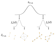
Figure 1 illustrates the predicted graph distribution in which $\hat{\mathcal{G}}_{T+h}$ is a function of predicted nodes $\hat{n}_{T+h}$ and $f_{u}(\bm{d})$. If we explore the predictions for different values of $\hat{n}_{T+h}$ and different upper bounds $u$, we get different graphs. Let $\gamma$ denote the quantile used to obtain $\hat{n}_{T+h}$ and $u$ denote the quantiles in $f_{u}(\bm{d})$. Then we can think of the graph $\hat{\mathcal{G}}_{T+h}$ as belonging to a graph distribution $\mathfrak{G}$ having parameters $\gamma$ and $u$:

$$\hat{\mathcal{G}}_{T+h}\sim\mathfrak{G}\left(\gamma,u\right)\,.$$

While these are explicit parameters, the coefficient scheme used to obtain $\xi_{ij}$, the methods used for predicting individual time series and their hyperparameters can also be considered as part of a wider parameter pool. While we use ARIMA models with automatic parameter selection (Hyndman & Khandakar, 2008) for time series prediction, LSTMs and other prediction methods can also be used.

Figure 1: A simple illustration of the predicted graph distribution in terms of $\gamma$ and $u$. The parameter $\gamma$ gives rise to different $\hat{n}_{T+h}$ values. The 2 graphs on the left have 4 nodes each, corresponding to a single $\gamma$ (or $\hat{n}_{T+h}$) value, but has different number of edges corresponding to different $u$ values. Similarly, the two graphs on the right have 7 nodes corresponding to a higher value of $\gamma$ with the rightmost graph having more edges due to a higher $u$.

3.5 Evaluation Metrics

We use the following evaluation metrics: 1. absolute node error $\frac{|\hat{n}_{T+h}-n_{T+h}|}{n_{T+h}}$ gives the absolute error of the predicted number of vertices compared to the actual as a ratio. 2. The adjacency matrix error computed as $\frac{\lVert\hat{A}_{T+h}-{A}_{T+h}\rVert}{\lVert{A}_{T+h}\rVert}$, where we pad $\hat{A}_{T+h}$ or ${A}_{T+h}$ with rows and columns of zeros to make their sizes sthe same. 3. Degree cosine similarity measuring the cosine similarity between the degree vectors of $\hat{\mathcal{G}}_{T+h}$ and ${\mathcal{G}}_{T+h}$. Again, we make the vectors compatible by inserting zeros at the end if the lengths differ.

4 Results

We investigate the performance of the network prediction algorithm on synthetic and real datasets.

4.1 Synthetic Experiments

For synthetic experiments, we generate a growing sequence of graphs $\left\{\mathcal{G}_{t}\right\}_{t=1}^{T}$ as follows. We start with a 5 node graph $\mathcal{G}_{1}$ and consider a node growth rate of $10\%$, i.e, graph $\mathcal{G}_{t+1}$ has $10\%$ more nodes compared to $\mathcal{G}_{t}$. To generate the graph sequence we consider 2 parameters: proportion of edges removed $\alpha$ and the proportion of edges increased $\beta$. From each $\mathcal{G}_{t}$ we randomly remove $\alpha|E_{t}|$ edges, where $|E_{t}|$ denotes the number of edges in $\mathcal{G}_{t}$. Thus, low values of $\alpha$ indicate a higher proportion of common edges between $\mathcal{G}_{t}$ and $\mathcal{G}_{t+1}$.

The parameter $\beta$ denotes the proportion of edges increased from $\mathcal{G}_{t}$ to $\mathcal{G}_{t+1}$, i.e., $\beta=(|E_{t+1}|-|E_{t}|)/|E_{t}|$. A larger $\beta$ value indicates a higher graph growth in terms of edges. Even though $\alpha$ and $\beta$ measure somewhat similar quantities, the difference is that $1-\alpha$ gives a similarity measure between $\mathcal{G}_{t}$ and $\mathcal{G}_{t+1}$ and $\beta$ gives a growth metric. Thus, they measure different aspects of graph evolution. Both edge deletion and addition are done randomly. Using this setting we predict graphs $\mathcal{G}_{T+h}$ for $T\in\{20,\ldots,24\}$ and $h\in\{1,\ldots,5\}$. We vary the parameters $\alpha$ and $\beta$ such that $\alpha,\beta\in\{0.1,0.2,\ldots,0.9\}$.

Figure 2: Predicted synthetic networks using a sequence of 24 graphs for $h\in\{1,3,5,7\}$ describing graphs at time steps 25, 27, 29 and 31. The predicted graphs have 85, 99, 113, 127 vertices and 470, 567, 643 and 716 edges respectively. Node color depicts the degree of the node, with darker nodes having higher degree.

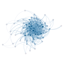
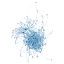
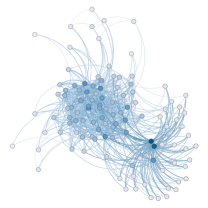
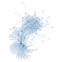
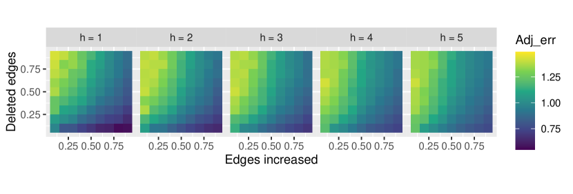
Figure 2 shows the predicted graphs at $T=24$ for time step $h\in\{1,3,5,7\}$ (predicted graphs at time steps 25, 27, 29 and 31) using $\gamma=0.5$ and $u=0.55$. The number of vertices in the predicted graphs increase with $h$ from 85 to 127, and the predicted edges increase from 470 to 716. Figure 3 shows the adjacency error for graph sequences with $T=20$ for different $h$ values. The results were similar for other $T$ values. We see that as we delete more edges the adjacency error increases, i.e., prediction becomes difficult. This is expected because it is easier to predict repeating patterns than random fluctuations. We also see that adjacency error decreases when $\beta$ (the proportion of edges increased), increases. This is because more dense graphs have more ones in the adjacency matrix, resulting in lower errors.

Figure 3: Results of the synthetic experiments for different time step predictions. The adjacency error of the predicted graphs for $T=20$ for $h\in\{1,\ldots,5\}$ for different values of $\alpha$ (proportions of deleted edges) and $\beta$ (proportion of edges increased).

4.2 Experiments using real-world datasets

We use the following datasets in this study.

• UCI Message (UCI): This dataset contains interactions between an online community of students at the University of California Irvine (Panzarasa et al., 2009). Each student is represented by a node and communications between students are represented by edges.

• EU-email (EU): This dataset was originally investigated by Leskovec et al. (2007) and was later made available by Paranjape et al. (2017). It contains the email network from a European research organisation. An edge $(u,v,t)$ signifies person $u$ sent person $v$ an email at time $t$.

• High School (HS): This dataset represents contact between students in a high school in Marseilles, France, in December 2013, collected using wearable sensors (Mastrandrea et al., 2015).

• Hypertext 2009 (HT09): This dataset was collected at the ACM HyperText 2009 Conference, where participants’ face-to-face interactions were recorded using RFID devices (Isella et al., 2011).

Each dataset is an anonymized edgelist of observations of the form $(u,v,t)$. For UCI and EU datasets we consider daily edges and for HS and HT09 datasets we consider hourly edges. Table 1 gives the total number of nodes, edges and density for each dataset for 35 time periods.

Table 1: Dataset summary

Dataset	Total Nodes	Total Edges	Density
UCI	1.3K	25.1K	$7.7\times 10^{-2}$
EU	857	102.6K	$9.7\times 10^{-3}$
HS	327	18.3K	$1.0\times 10^{-2}$
HT09	113	3.6K	$3.3\times 10^{-2}$

Figure 4: UCI-Message predicted networks using a sequence of 20 graphs ($T=20$) for time steps $h\in\{1,3,5\}$. The predicted graphs have 873, 963, 1054 vertices and 924, 1059, 1152 edges respectively. Node color depicts node degree with darker colors depicting higher degree.

Figure 5: Node error of the predicted graphs $\hat{\mathcal{G}}_{T+h}$ for $T\in\{20,\ldots,30\}$ and $h\in\{1,\ldots,5\}$.

Table 2: Results summary

Dataset	Form	Adjacency Error							Degree Cosine Similarity
		$h=1$	$h=2$	$h=3$	$h=4$	$h=5$	Err1.		$h=1$	$h=2$	$h=3$	$h=4$	$h=5$
	F2C3	1.91	2.03	2.10	2.14	2.15	26.15		0.50	0.44	0.43	0.41	0.38
UCI	F2C2	2.02	2.12	2.18	2.22	2.22	26.15		0.10	0.08	0.05	0.05	0.04
	F1C3	3.08	3.35	3.53	3.63	3.69	26.15		0.53	0.48	0.47	0.46	0.43
	F1C2	34.40	34.59	34.62	34.33	34.06	26.15		0.33	0.32	0.32	0.33	0.33
	F2C3	1.94	1.49	1.56	2.27	2.60	37.28		0.60	0.69	0.67	0.59	0.55
EU	F2C2	2.24	1.83	1.89	2.56	2.87	37.28		0.03	0.03	0.04	0.03	0.02
	F1C3	2.67	2.63	2.79	3.63	4.34	37.91		0.62	0.64	0.63	0.60	0.56
	F1C2	36.65	32.24	32.32	39.83	45.54	37.91		0.40	0.43	0.43	0.40	0.38
	F2C3	1.56	1.54	1.54	1.52	1.46	11.68		0.67	0.67	0.67	0.69	0.69
HS	F2C2	1.83	1.80	1.80	1.78	1.72	11.68		0.16	0.17	0.17	0.18	0.19
	F1C3	2.07	2.30	2.48	2.58	2.55	11.68		0.72	0.72	0.70	0.72	0.73
	F1C2	11.55	11.57	11.60	11.41	10.82	11.68		0.64	0.65	0.65	0.67	0.68
	F2C3	2.98	4.43	4.57	4.69	4.66	20.72		0.61	0.55	0.52	0.50	0.50
HT09	F2C2	3.11	4.54	4.69	4.82	4.79	20.72		0.25	0.22	0.23	0.22	0.16
	F1C3	3.87	6.31	7.20	7.71	7.92	20.72		0.68	0.60	0.56	0.53	0.53
	F1C2	13.11	19.24	20.03	20.94	20.91	20.72		0.55	0.51	0.49	0.47	0.47

To standardize computations across datasets we predicted graphs $\hat{\mathcal{G}}_{T+h}$ for $T\in\{20,\ldots,30\}$ and $h\in\{1,2,3,4,5\}$. Predictions were carried out for all combinations of $T$ and $h$. We used Formulations 1 and 2 (F1 and F2) with binary and proportional coefficients (C2 and C3). For all configurations we used 0.9 as the upper bound $u$ in $f_{u}(\bm{d})$ and for proportional coefficients C3, we used $\lambda=0.001$.

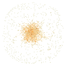
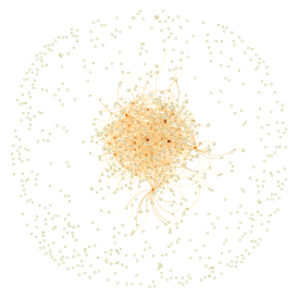
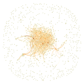
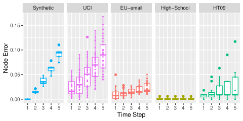
Figure 4 shows 3 predicted graphs for UCI dataset for $h\in\{1,3,5\}$ at $T=20$ using Formulation 2, coefficients C3, $\gamma=0.5$, $u=0.9$ and $\lambda=0.001$. The nodes and edges in predicted graphs increase with $h$. Figure 5 shows the node error of the datasets for different prediction time-steps $h$. For each time-step $h$ we have 11 predictions for $T\in\{20,\ldots,30\}$ from different graphs $\hat{\mathcal{G}}_{T+h}$. For all datasets apart from High-School dataset we see that the node error increases with the prediction time-step $h$. This is to be expected as it is difficult to forecast further into the future. The High-School dataset is an exception because it has a smaller node growth rate that plateaus after some time.

Table 2 gives the prediction results for these datasets for $\gamma=0.5$ and $u=0.9$. For each dataset and configuration we list the adjacency error and degree cosine similarity for all $h$ values. As there are 11 predictions for each $h$ from different $T$ values we take the average over $T$. As we saw from Table 1 the graph densities are in the $10^{-2}$ range. Thus only this proportion of entries in the adjacency matrix have ones. Therefore, it is quite easy to get an adjacency error greater than 1. To give some perspective of the range of adjacency errors, we compute the error if $\hat{A}_{T+h}-{A}_{T+h}$ is a matrix of all ones. This is not an upper bound because we take the size of $\hat{A}_{T+h}$ to be equal to that of ${A}_{T+h}$ in this computation. However, it is still a useful heuristic because it increases our understanding of the range of adjacency errors. This error is labeled as ERR1 in Table 2.

As general trends we see that the adjacency error increases and the degree cosine similarity decreases as $h$ increases. The configuration F2C3 achieves the best adjacency errors for all 4 datasets followed by F2C2 and F1C3. F1C2 has very large adjacency errors, often greater than ERR1 values. The difference between F1 and F2 is that F2 includes a constraint for total additional edges. The coefficient schemes C2 uses binary coefficients and C3 uses proportional coefficients. In terms of adjacency error, the difference between F2C3 and F1C2 is far greater than changing one setting – either F2 to F1, or C3 to C2 – at a time. The degree cosine similarity is best for F1C3 closely followed by F2C3. We see that F2C2 has poor degree similarity, even though the adjacency error maybe low. From this we can see proportional coefficients (C3) are more important for better predictions than constraining the total edges.

The current formulations solve an optimization problem of $n(n-1)/2$ variables for a graph with $n$ vertices. Thus, the efficiency of the optimization algorithm can be improved. On a different note, we can explore the predictive distribution discussed in Section 3.4 by changing parameters $\gamma$ and $u$. We illustrate graphs with different $\gamma$ and $u$ values in Appendix C.

5 Conclusion

We have presented a method to predict graphs at future time points from a time series of graphs . Our prediction can include new nodes and edges. The proposed method uses time series methods to predict the node degree and linear programming techniques from flux balance analysis to obtain the future graph. We investigated the utility of our method on synthetic and real datasets. This work focused on predicting the exact graph, i.e., our methodology did not explore assumptions of exchangeability of graph vertices or edges. Investigating prediction methods for exchangeable graphs and improving the efficiency of the optimization algorithm are future research avenues.

Acknowledgments

I sincerely thank Dr Cheng Soon Ong for helpful discussions.

Appendix A Additional methodology details

Theorem 3.2 Let $\mathcal{U}\,,\bm{u}\in\mathcal{U}$ describe the solution space of the optimization problem described in Formulation 1. Then the cardinality of $\mathcal{U}$, denoted by $\left|\mathcal{U}\right|$ satisfies the following bounds

$$0<C_{1}\leq\left|\mathcal{U}\right|\leq C_{2}$$

where $C_{1}$ and $C_{2}$ depend on $n$ and $f_{u}(\bm{d})$.

Proof.

For the optimization problem in Formulation 1 we have

$$S\bm{u} \leq f_{u}\left(\bm{d}\right)$$ (9)

$$\text{giving us }\bm{1}^{T}S\bm{u} \leq\bm{1}^{T}f_{u}\left(\bm{d}\right)=\sum_{i}f_{u}(\hat{d}_{i})$$ (10)

where equation (10) denotes a single constraint comprising the addition of the individual constraints in equation (9). Suppose $\bm{u}_{j}$ satisfies the individual constraints in equation (9). Then $\bm{u}_{j}$ satisfies the summed constraint in equation (10). Thus $\mathcal{U}\subset\mathcal{U}_{\text{sum}}$ where $\mathcal{U}_{\text{sum}}$ denotes the solution space of the summed constraint.

We consider $\bm{u}_{j}\in\mathcal{U}_{\text{sum}}$ as a binary string. Thus, the number of binary strings in $\mathcal{U}_{\text{sum}}$ is an upper bound for $\left|\mathcal{U}\right|$. From Lemma 3.3 we know $\sum_{k}s_{kl}=\{0,2\}$ for all $k$. As a result we have

$$\bm{1}^{T}S=2\bm{B}^{T}$$

where $\bm{1}^{T}$ is a $1\times n$ row vector and $\bm{B}^{T}$ is an $1\times n(n-1)/2$ binary row vector (containing ones and zeros). Substituting this in equation $\eqref{eq:2}$ we get

$$2\bm{B}^{T}\bm{u}\leq\sum_{i}f_{u}(\hat{d}_{i})\iff\bm{B}^{T}\bm{u}\leq\frac{1}{2}\sum_{i}f_{u}(\hat{d}_{i})$$ (11)

where the hyperplane describing the constraint now has coefficients equal to 1. The number of ones in $\bm{B}$ is equal to the number of edges in the union graph $\mathcal{G}_{U}$. Let $c_{3}=\lfloor\frac{1}{2}\sum_{i}f_{u}(\hat{d}_{i})\rfloor$ and $m$ denote the number of ones in $\bm{B}$, which is the length of the binary string we consider. Then the number of binary strings with $k$ ones is ${m\choose k}$. To satisfy the constraint in equation (10) we can have up to $c_{3}$ ones giving us a total of

$${m\choose 1}+{m\choose 2}+\cdots+{m\choose c_{3}}=C_{2}$$ (12)

possible binary sequences comprising the upper bound.

For the lower bound we consider the order statistics of $f_{u}(\bm{d})$ in reverse (decreasing) order. Let $f_{u}(\bm{d})_{(k)}$ be the $k$th reverse order statistic of $f_{u}(\bm{d})$ and let $\bm{v}_{(k)}$ be the corresponding vertex. Let $\eta_{i}$ be the number of inequalities (corresponding to vertices) in equation (10) with $f_{u}(d_{k})=i-1$. Thus, $\eta_{1}$ gives the number of vertices with an upper bound degree 0. To give some intuition, $\eta_{i}$ focuses on low upper bound degree vertices. Let $k$ be the largest integer that satisfies the following inequalities:

$$\eta_{k}+k+f_{u}(\bm{d})_{(k)} \leq n$$ (13)

$$f_{u}(\bm{d})_{(1)}+f_{u}(\bm{d})_{(2)}+\cdots+f_{u}(\bm{d})_{(k)} \leq\frac{1}{2}\sum_{i}f_{u}(d_{i})$$ (14)

The first inequality is about selecting vertices to draw edges. When $k=1$, we consider the vertex $\bm{v}_{(1)}$. There are $n-1$ vertices available to connect with $\bm{v}_{(1)}$ if the upper bound of all vertices are strictly positive. But if certain vertices have a zero upper bound, we need to remove those vertices, when considering edges with $\bm{v}_{(1)}$, i.e., then we consider $n-1-\eta_{1}$ vertices. The term $f_{u}(\bm{d})_{(k)}$ denotes the maximum number of edges we can draw as we will see later.

The second inequality specifies the number of inequalities $k$ to consider to obtain a lower bound of $|\mathcal{U}|$. As sum of the degrees is twice the sum of edges for non-weighted graphs, we don’t need to consider all the vertices specified by the inequalities. Rather, we only need to focus on the top $\bm{v}_{k}$ vertices with upper bounds $\sum_{i}f_{u}(\bm{d})_{(i)}$ adding up to the total number of edges. We note that both the upper and lower bounds of $|\mathcal{U}|$ are not strict upper and lower bounds.

Let us first consider the case when these 2 inequalities are satisfied. We note that the assumptions detailed by the inequalities are reasonable and satisfied for at least $k=1$ because $n$ is generally much larger than $f_{u}(\bm{d})_{(1)}$, the upper bound degree of $\bm{v}_{(1)}$, with $\eta_{1}$ small, satisfying inequality (13) and the largest upper bound degree $f_{u}(\bm{d})_{(1)}$ is generally less than all the edges a graph can have or its upper bound $\frac{1}{2}\sum_{i}f_{u}(d_{i})$.

We start with $\bm{v}_{(1)}$ the vertex corresponding to $f_{u}(\bm{d})_{(1)}$, i.e., the vertex with the highest upper bound degree. This vertex can have a maximum number of $f_{u}(\bm{d})_{(1)}$ edges. First we need to select another vertex to draw an edge from $\bm{v}_{(1)}$. There are $n-1-\eta_{1}$ such vertices because the graph has $n$ vertices and $u_{1}$ vertices with upper bound degree 0. An edge can be made from $\bm{v}_{(1)}$ to any of these vertices. Thus, the number of graphs with 1 edge from $\bm{v}_{(1)}$ are ${{n-1-\eta_{1}}\choose 1}$. To draw 2 edges from $\bm{v}_{(1)}$ we need to select 2 vertices from $n-1-\eta_{1}$. We note that it is $(n-1-\eta_{1})$ and not $(n-1-\eta_{2})$ when we are using vertex $\bm{v}_{(1)}$ because we are counting graphs with 2 edges separately from graphs with 1 edge. The number of graphs with 2 edges from $\bm{v}_{(1)}$ are ${{n-1-\eta_{1}}\choose 2}$. Therefore, the number of graphs having upto a maximum of $f_{u}(\bm{d})_{(1)}$ edges for $\bm{v}_{(1)}$ is

$$g_{1}={{n-1-\eta_{1}}\choose 1}+{{n-1-\eta_{1}}\choose 2}+\cdots+{{n-1-\eta_{1}}\choose{f_{u}(\bm{d})_{(1)}}}\,.$$ (15)

We note that each of these graphs not only satisfy the largest constraint (with $f_{u}(\bm{d})_{(1)}$ upper bound degree), but they satisfy the other constraints as well because they draw edges with vertices having degree $\geq 1$. Having considered the vertex with the largest upper bound degree, we focus on the second largest upper bound degree $f_{u}(\bm{d})_{(2)}$. When constructing edges from $\bm{v}_{(2)}$ we only consider vertices other than $\bm{v}_{(1)}$ and vertices that have $f_{u}(d_{i})>1$ (there are $\eta_{2}$ such vertices) because we are interested in a lower bound. If we were counting all the graphs, then we need to consider the case when $\bm{v}_{(1)}$ and $\bm{v}_{(2)}$ have an edge and when they don’t and compute all possible combinations. As we’re interested in a lower bound we simply focus on the other vertices. We have $n-2-\eta_{2}$ such vertices to choose from to draw an edge from $\bm{v}_{(2)}$. The degree of $\bm{v}_{(2)}$ is bounded by $f_{u}(\bm{d})_{(2)}$. But we do not know if there is an edge between $\bm{v}_{(1)}$ and $\bm{v}_{(2)}$. To get a lower bound we suppose there is an edge and only allocate up to $f_{u}(\bm{d})_{(2)}-1$ edges from $\bm{v}_{(2)}$.

The number of graphs satisfying the second largest constraint are

$$g_{2}\geq{{n-2-\eta_{2}}\choose 1}+{{n-2-\eta_{2}}\choose 2}+\cdots+{{n-2-\eta_{2}}\choose{f_{u}(\bm{d})_{(2)}-1}}\,.$$ (16)

Again, each of these graphs satisfy the other constraints as well. Similarly, the number of graphs satisfying the $k$th largest constraint satisfy

$$g_{k}\geq{{n-k-\eta_{k}}\choose 1}+{{n-k-\eta_{k}}\choose 2}+\cdots+{{n-k-\eta_{k}}\choose{f_{u}(\bm{d})_{(k)}-k+1}}\,.$$ (17)

For any vertex $\bm{v}_{(i)}$ if $f_{u}(\bm{d})_{(i)}-i+1\leq 0$ then we can stop at $\ell$ such that $f_{u}(\bm{d})_{(i)}-\ell+1=1$, i.e., stop early in inequality (17) without computing all the terms.

Next we consider the union of graphs satisfying equations (15), (16) and (17). The union of any graph specified in equation (15) with a graph in equation (16) still satisfies all the constraints because graphs in (16) do not draw edges to $\bm{v}_{(1)}$ and so on. Thus, the the graphs satisfying all the constraints is the union of all different combinations of graphs described in each equation/inequality. Therefore we obtain the following lower bound:

$$C_{1}=g_{1}g_{2}\ldots g_{k}$$ (18)

Suppose the assumptions detailed in inequalities (13) and (14) are not satisfied. Inequality (14) not being satisfied has minimal impact as we will illustrate now. Suppose

$$f_{u}(\bm{d})_{(1)}\geq\frac{1}{2}\sum_{i}f_{u}(d_{i})\,.$$

Then we can compute $g_{1}$ graphs as detailed in (15) and let $C_{1}=g_{1}$.

The assumption in inequality (13) has a more serious effect if it is not met. Suppose $n\leq\eta_{1}+1$, which results in inequality (13) not being met in the most radical way. Then, we have $\eta_{1}\geq n-1$ but as there are only $n$ vertices this implies $\eta_{1}=n-1$ or $\eta_{1}=n$ giving us the extreme situation forcing $f_{u}(\bm{d})=\bm{0}$ when $\eta_{1}=n$. This situation forces there to be no edges giving us the edgeless graph consisting of vertices alone. Thus in this case

$$C_{1}=1\,.$$

Let us consider another situation where $f_{u}(\bm{d})=\bm{1}$. While noting it is unusual to have all the upper bound degrees to be 1, we can still find multiple graphs satisfying this constraint. The first edge can be selected from ${n\choose 2}$ pairs of vertices. The next edge can be selected from ${{n-2}\choose 2}$ pairs of vertices and so on. This results in $\lfloor n/2\rfloor$ edges, which can be ordered in ${\lfloor n/2\rfloor}!$ ways. Thus, we would have

$$C_{1}=\frac{{n\choose 2}{{n-2}\choose 2}\cdots{{q}\choose 2}}{{\lfloor\frac{n}{2}\rfloor}!}\,,$$

where $q=2$ or $q=3$ depending on the graph giving us $C_{1}$ graphs as the lower bound for this set of constraints. For real graphs it is extremely unlikely to obtain $f_{u}(\bm{d})=\bm{1}$ or $f_{u}(\bm{d})=\bm{0}$. Thus, mostly we would have a lower bound expressed by equation (18). ∎

Appendix B Synthetic Experimental Results

Figure 6: Degree cosine similarity and node error of synthetic experiments.

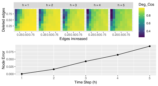
Figure 6 shows the degree cosine similarity and node error of synthetic experiments for different time steps $h\in\{1,\ldots,5\}$. As the time step $h$ increases the node error increases and the degree cosine similarity generally decreases. The degree cosine similarity depends on $\alpha$, the proportion of edges deleted and $\beta$ the proportion of edges increased. The degree cosine similarity decreases as $\alpha$ increases but generally increases as $\beta$ increases.

Appendix C Results from Real Datasets

C.1 Graphs from the predictive distribution

Figure 7 shows 3 predicted graphs for UCI-Message dataset for different $\gamma$ and $u$ values. The colors in UCI-Message represent eccentricity of nodes (the maximum distance to other nodes) computed for each node’s connected component with darker colors used for most eccentric nodes and light yellow used for unconnected nodes. The graph predictions are using a time series of graphs with $T=30$ and $h=1$. The leftmost graph shows the predicted network with $\gamma=0.2$ and $u=0.55$. The middle graph correspond to $\gamma=0.5$ and $u=0.95$. The rightmost graph correspond to $\gamma=0.8$ and $u=0.95$. The number of predicted nodes in graphs from left to right are 1113, 1133 and 1166 respectively. This is because the corresponding $\gamma$ values $\{0.2,0.5,0.8\}$ give rise to different number of nodes in the predicted graph. The predicted graphs from left to right have 494, 646, and 646 edges respectively. This is a result of the $u$ values $\{0.55,0.95,0.95\}$. Even though $\gamma$ values in the middle and the rightmost graph are different (0.5 and 0.8) the number of edges is the same because we are using Formulation 2, which constraints the total number of edges to the predicted total number of edges. Had we used Formulation 1, the edges would have increased as well. The illustrated graphs are specific instances of the distribution of predicted graphs, and similar graphs can be obtained by varying $\gamma$ and $u$ values.

Figure 7: UCI-Message predicted networks for different values of $\gamma$ and $u$. Nodes colored by node eccentricity with yellow for unconnected and blue for most eccentric nodes.

Figure 8: EU-Email predicted networks for $\gamma=0.5$ and $u\in\{0.55,0.80,0.95\}$. Nodes coloured by node eccentricity.

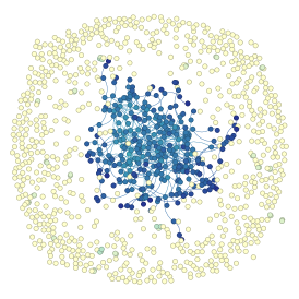
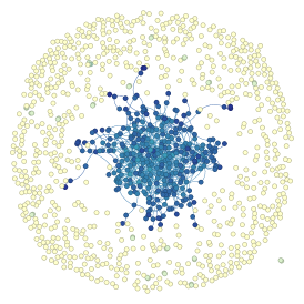
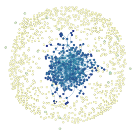
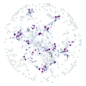
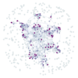
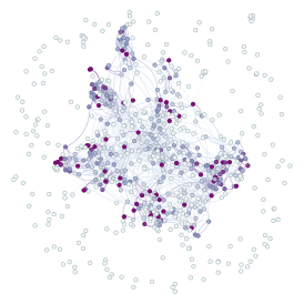
Figure 8 shows 3 predicted graphs for the EU-Email dataset for $\gamma=0.5$ and $u\in\{0.55,0.80,0.95\}$ from a time series of graphs with $T=30$ and $h=1$. Again nodes are colored by their eccentricity with unconnected nodes colored the lightest and most eccentric nodes colored the darkest. All 3 predicted graphs have 706 nodes corresponding to $\gamma=0.5$. The number of edges in the leftmost, middle and the rightmost graphs are 916, 1118 and 1377 respectively. The number of edges increase because the upper bound $u$ increased from left to right.

References

- (1)
- Bai et al. (2019) Bai, Y., Ding, H., Qiao, Y., Marinovic, A., Gu, K., Chen, T., Sun, Y. & Wang, W. (2019), Unsupervised inductive graph-level representation learning via graph-graph proximity, in ‘IJCAI International Joint Conference on Artificial Intelligence’, Vol. 2019-August, pp. 1988–1994.
-
Barros et al. (2021)
Barros, C. D. T., Mendonça, M. R. F., Vieira, A. B. & Ziviani, A. (2021), ‘A survey on embedding dynamic graphs’, ACM Comput. Surv. 55(1).
https://doi.org/10.1145/3483595 - Bazaraa et al. (2011) Bazaraa, M. S., Jarvis, J. J. & Sherali, H. D. (2011), Linear programming and network flows, John Wiley & Sons.
- Cai et al. (2016) Cai, D., Campbell, T. & Broderick, T. (2016), Edge-exchangeable graphs and sparsity, in D. Lee, M. Sugiyama, U. Luxburg, I. Guyon & R. Garnett, eds, ‘Advances in Neural Information Processing Systems’, Vol. 29, Curran Associates, Inc.
Chen et al. (2022)
Chen, J., Wang, X. & Xu, X. (2022), ‘GC-LSTM: graph convolution embedded LSTM for dynamic network link prediction’, Applied Intelligence 52(7), 7513–7528.
https://arxiv.org/abs/1812.04206v2 - Chen et al. (2021) Chen, J., Zhang, J., Xu, X., Fu, C., Zhang, D., Zhang, Q. & Xuan, Q. (2021), ‘E-LSTM-D: A Deep Learning Framework for Dynamic Network Link Prediction’, IEEE Transactions on Systems, Man, and Cybernetics: Systems 51(6), 3699–3712.
- Divakaran & Mohan (2020) Divakaran, A. & Mohan, A. (2020), ‘Temporal Link Prediction: A Survey’, New Generation Computing 38(1), 213–258.
- Galke et al. (2021) Galke, L., Franke, B., Zielke, T. & Scherp, A. (2021), Lifelong learning of graph neural networks for open-world node classification, in ‘2021 International Joint Conference on Neural Networks (IJCNN)’, pp. 1–8.
- Getoor et al. (2003) Getoor, L., Friedman, N., Koller, D. & Taskar, B. (2003), ‘Learning probabilistic models of link structure’, Journal of Machine Learning Research 3(4-5), 679–707.
Goyal et al. (2017)
Goyal, P., Kamra, N., He, X. & Liu, Y. (2017), DynGEM: Deep Embedding Method for Dynamic Graphs, in ‘3rd International Workshop on Representation Learning for Graphs (ReLiG), IJCAI’.
http://arxiv.org/abs/1805.11273 - Hamilton et al. (2017) Hamilton, W. L., Ying, R. & Leskovec, J. (2017), Inductive representation learning on large graphs, in ‘Advances in Neural Information Processing Systems’, Vol. 2017-Decem, pp. 1025–1035.
- Han, Karunasekera & Leckie (2021) Han, Y., Karunasekera, S. & Leckie, C. (2021), Continual learning for fake news detection from social media, in ‘Artificial Neural Networks and Machine Learning – ICANN 2021: 30th International Conference on Artificial Neural Networks, Bratislava, Slovakia, September 14–17, 2021, Proceedings, Part II’, p. 372–384.
- Han, Ding, Ma, Gu & Tresp (2021) Han, Z., Ding, Z., Ma, Y., Gu, Y. & Tresp, V. (2021), Learning Neural Ordinary Equations for Forecasting Future Links on Temporal Knowledge Graphs, in ‘EMNLP 2021 - 2021 Conference on Empirical Methods in Natural Language Processing, Proceedings’, pp. 8352–8364.
- Hyndman & Khandakar (2008) Hyndman, R. J. & Khandakar, Y. (2008), ‘Automatic time series forecasting: the forecast package for R’, Journal of Statistical Software 26(3), 1–22.
Isella et al. (2011)
Isella, L., Stehlé, J., Barrat, A., Cattuto, C., Pinton, J.-F. & Van den Broeck, W. (2011), ‘What’s in a crowd? Analysis of face-to-face behavioral networks’, Journal of Theoretical Biology 271(1), 166–180.
https://www.sciencedirect.com/science/article/pii/S0022519310006284 - Kazemi et al. (2020) Kazemi, S. M., Goel, R., Jain, K., Kobyzev, I., Sethi, A., Forsyth, P. & Poupart, P. (2020), ‘Representation learning for dynamic graphs: A survey’, Journal of Machine Learning Research 21.
- Kim et al. (2022) Kim, S., Yun, S. & Kang, J. (2022), DyGRAIN: An Incremental Learning Framework for Dynamic Graphs, in ‘IJCAI International Joint Conference on Artificial Intelligence’, pp. 3157–3163.
- Leskovec et al. (2007) Leskovec, J., Kleinberg, J. & Faloutsos, C. (2007), ‘Graph evolution: Densification and shrinking diameters’, ACM Transactions on Knowledge Discovery from Data 1(1).
- Luo et al. (2023) Luo, L., Haffari, G. & Pan, S. (2023), Graph sequential neural ode process for link prediction on dynamic and sparse graphs, in ‘Proceedings of the Sixteenth ACM International Conference on Web Search and Data Mining’, WSDM ’23, p. 778–786.
- Ma et al. (2018) Ma, X., Sun, P. & Wang, Y. (2018), ‘Graph regularized nonnegative matrix factorization for temporal link prediction in dynamic networks’, Physica A: Statistical Mechanics and its Applications 496, 121–136.
- Mastrandrea et al. (2015) Mastrandrea, R., Fournet, J. & Barrat, A. (2015), ‘Contact patterns in a high school: A comparison between data collected using wearable sensors, contact diaries and friendship surveys’, PLoS ONE 10(9).
- Orth et al. (2010) Orth, J. D., Thiele, I. & Palsson, B. O. (2010), ‘What is flux balance analysis?’, Nature Biotechnology 28(3), 245–248.
- Panzarasa et al. (2009) Panzarasa, P., Opsahl, T. & Carley, K. M. (2009), ‘Patterns and dynamics of users’ behavior and interaction: Network analysis of an online community’, Journal of the American Society for Information Science and Technology 60(5), 911–932.
Paranjape et al. (2017)
Paranjape, A., Benson, A. R. & Leskovec, J. (2017), Motifs in temporal networks, in ‘Proceedings of the Tenth ACM International Conference on Web Search and Data Mining’, WSDM ’17, Association for Computing Machinery, New York, NY, USA, p. 601–610.
https://doi.org/10.1145/3018661.3018731 - Pareja et al. (2020) Pareja, A., Domeniconi, G., Chen, J., Ma, T., Suzumura, T., Kanezashi, H., Kaler, T., Schardl, T. B. & Leiserson, C. E. (2020), EvolveGCN: Evolving graph convolutional networks for dynamic graphs, in ‘AAAI 2020 - 34th AAAI Conference on Artificial Intelligence’, pp. 5363–5370.
- Qu et al. (2020) Qu, L., Zhu, H., Duan, Q. & Shi, Y. (2020), Continuous-Time Link Prediction via Temporal Dependent Graph Neural Network, in ‘The Web Conference 2020 - Proceedings of the World Wide Web Conference, WWW 2020’, pp. 3026–3032.
- Rossi et al. (2020) Rossi, R. A., Zhou, R. & Ahmed, N. K. (2020), ‘Deep Inductive Graph Representation Learning’, IEEE Transactions on Knowledge and Data Engineering 32(3), 438–452.
Sankar et al. (2020)
Sankar, A., Wu, Y., Gou, L., Zhang, W. & Yang, H. (2020), Dysat: Deep neural representation learning on dynamic graphs via self-attention networks, in ‘Proceedings of the 13th International Conference on Web Search and Data Mining’, WSDM ’20, Association for Computing Machinery, New York, NY, USA, p. 519–527.
https://doi.org/10.1145/3336191.3371845 - Su et al. (2023) Su, J., Zou, D., Zhang, Z. & Wu, C. (2023), Towards Robust Graph Incremental Learning on Evolving Graphs, in ‘International Conference on Machine Learning, Poster’.
- Tan et al. (2022) Tan, Z., Ding, K., Guo, R. & Liu, H. (2022), Graph few-shot class-incremental learning, in ‘Proceedings of the Fifteenth ACM International Conference on Web Search and Data Mining’, WSDM ’22, p. 987–996.
- Trivedi et al. (2019) Trivedi, R., Farajtabar, M., Biswal, P. & Zha, H. (2019), ‘Dyrep: Learning representations over dynamic graphs’.
- Wang et al. (2020) Wang, J., Song, G., Wu, Y. & Wang, L. (2020), Streaming Graph Neural Networks via Continual Learning, in ‘International Conference on Information and Knowledge Management, Proceedings’, pp. 1515–1524.
- Xu et al. (2020) Xu, Y., Zhang, Y., Guo, W., Guo, H., Tang, R. & Coates, M. (2020), Graphsail: Graph structure aware incremental learning for recommender systems, in ‘Proceedings of the 29th ACM International Conference on Information & Knowledge Management’, CIKM ’20, p. 2861–2868.
- Yang et al. (2016) Yang, Z., Cohen, W. W. & Salakhutdinov, R. (2016), Revisiting semi-supervised learning with graph embeddings, in ‘33rd International Conference on Machine Learning, ICML 2016’, Vol. 1, pp. 86–94.
- Yin et al. (2021) Yin, H., Hu, W., Zhang, Z., Lou, J. & Miao, M. (2021), ‘Incremental multi-view spectral clustering with sparse and connected graph learning’, Neural Networks 144, 260–270.
You et al. (2022)
You, J., Du, T. & Leskovec, J. (2022), Roland: Graph learning framework for dynamic graphs, in ‘Proceedings of the 28th ACM SIGKDD Conference on Knowledge Discovery and Data Mining’, KDD ’22, Association for Computing Machinery, New York, NY, USA, p. 2358–2366.
https://doi.org/10.1145/3534678.3539300 - Yuan et al. (2021) Yuan, Z., Liu, H., Liu, J., Liu, Y., Yang, Y., Hu, R. & Xiong, H. (2021), Incremental spatio-temporal graph learning for online query-poi matching, in ‘Proceedings of the Web Conference 2021’, WWW ’21, p. 1586–1597.
- Zhang et al. (2022) Zhang, X., Song, D. & Tao, D. (2022), CGLB: Benchmark Tasks for Continual Graph Learning, in ‘Proceedings of the 36th Conference on Neural Information Processing Systems (NeurIPS 2022) Track on Datasets and Benchmarks’, Vol. 35.