Shear deformation in CuZr metallic glass: A statistical and complex network analysis

Abstract

We have implemented a complex network description for metallic glasses, able to predict the elasto-plastic regime, the location of shear bands and the statistics that controls the plastic events that originate in the material due to a deformation process. By means of molecular dynamics simulations, we perform a shear deformation test, obtaining the stress-strain curve for CuZr metallic glass samples. The atomic configurations of the metallic glass are mapped to a graph, where a node represents an atom whose stress/strain is above a certain threshold, and edges are connections between existing nodes at consecutive timesteps in the simulation. We made a statistical study of some physical descriptors such as shear stress, shear strain, volumetric strain and non-affine displacement to use them as construction tools for complex networks. We have calculated their probability density functions, skewness, kurtosis and gini coefficient to analyze the inequality of the distributions. We study the evolution of the resulting complex network, by computing topological metrics such as degree, clustering coefficient, betweenness and closeness centrality as a function of the strain. We have obtained correlations between the physical phenomena produced by the deformation with the data recorded by these metrics. By means the visual representation of the networks, we have also found direct correlations between metrics and the local atomic shear strain, so that they are able to predict the location of shear bands, as well as the formation of highly connected and interacting communities, which we interpret as shear transformation zones. Our results suggest that the complex network approach has interesting capabilities for the description of mechanical properties of metallic glasses.

1 Introduction

Metallic glasses (MGs) are non-crystalline solids with very interesting physical, chemical [1], magnetic [2] and mechanical [3] properties for their technological applications [4, 5]. After the synthesis of the first MG in 1960 [6] and the development of large-scale metallic glasses (BMGs) in 1993 [7, 8], the theoretical and experimental studies of these materials have been an area of intense research [9]. The disordered nature of MGs causes them to exhibit excellent mechanical properties, such as high yield strength, large elastic strain limits, good wear resistance, among others [10]. They are even able to deform elastically to a strain limit greater than 2%, which is an order of magnitude higher than in their crystalline metallic form. However, it has been observed that BMGs suffers brittle fracture due to its limited ductility under mechanical tests [11, 12], which has inhibited its direct use as a structural material [13].

The mechanical behavior and plastic deformation in BMGs, is still a topic that keeps scientists and engineers very fascinated. It is well known that when a load is applied to a MG sample, after the elastic limit is reached, it immediately undergoes catastrophic failure. Thus, in contrast to its crystalline counterpart, where dislocations are the main carriers of plasticity, MGs do not have this property due to the absence of grain boundaries, causing them to be materials with high mechanical resistance but brittle [3, 9]. So far, there is no theory that explains the physics behind these events. It has been hypothesized that this behavior can be explained by the location of structural and dynamical heterogeneities called shear transformation zones (STZs), where a pair of atoms ($\approx$ 8–20) rearrange to adapt to the applied strain [14, 15]. These STZs are initially randomly distributed along the sample, but gradually begin to correlate both spatially and temporally, coalescing to give rise to shear bands (SBs) [16]. The localization, or the formation, of a dominant SB results in catastrophic failure, and the dynamics of this mechanism are thought to be key to understanding the mechanical behavior of MGs [17]. In fact, several experimental and theoretical works have been devoted to the problem of avoiding the localization of SBs to generate a homogeneous plastic deformation in the material, improve its mechanical properties, and prevent fracture [18, 19].

Usually, to study the physical properties of materials, statistical mechanics is used through atomic simulations. However, new mathematical tools have emerged to be used to study complexity and "discretizable" systems. We are referring to the concepts of complex networks (CNs) and graph theory [20, 21], where their application stands out in different fields of science [22, 23, 24, 25]. In physics, these tools have proven useful for describing complex systems, by providing a new perspective for their study, and revealing features which would be otherwise difficult to find with more traditional methods. For instance, researchers have used network analysis to examine the structure and behavior of granular materials [26], representing force-chain interactions via networks. Similarly, network analysis has been employed to study plastic deformation in metals, calculating the stress-strain curve as a time series and comparing it with various topological measures[27]. Several authors have applied components of complex network analysis to study the rheological properties, rejuvenation behavior, and local structure of metallic glasses. For example, computing the clustering coefficient[28, 29, 30]. Additionally, it has been used successfully in the study of earthquakes [25, 31, 32]. By means of a CN representation of the spatiotemporal evolution of seismic events, it has been possible to show universal characteristics of seismicity in different geological zones [31], investigate the transition involved in the occurence of a large earthquake [33] and the relationship between the $b$-value and coupling in a seismic zone [34]. A similar approach for CN construction has been followed to study solar flares [22] and the evolution of solar activity, as measured by sunspots appearance in the solar photosphere, along the 23rd solar cycle [35], thus showing the versatility of this technique to extract valuable information about energy release events in physical systems. Interestingly, a systematic research on complex system approaches for MGs subjected to an external deformation, is still needed. Since glass theory is still an underdeveloped field, CN analysis may provide a different and useful viewpoint to the mechanical response of amorphous solids.

In this research, we develop a microscopic study of the plastic deformation of a MG through computational simulations and complex networks techniques. Using classical molecular dynamics (MD) simulations, a sample of Cu₅₀Zr₅₀ MG is subjected to shear deformation [36]. MD simulations allow us to monitor atomic level events that appear when applying the shear deformation in the material. Based on these data, provided by MD simulations, a graph formed by nodes and vertices is built, and the time series of these graphs form the complex network of the system, being an abstract representation of the spatiotemporal evolution of stress. For these networks, various topological measurements are calculated for the networks, and compared with the physical process represented by atomistic simulations. In section II, we describe the details of the MD simulations, the deformation process and the physical observables obtained. In section III we present a statistical study of some physical descriptors that are used for CNs. We computed the spatial distributions and probability densities of these descriptors, as well as their moments, Lorenz curves, and Gini coefficient. In section IV we explain the construction process of the graphs and present the topological metrics that are used to characterize the resulting networks. In Section V the results are presented, and finally in Section VI the conclusions are drawn.

2 Simulations details

To study the microscopic phenomena involved in the plastic deformation of a MG, we perform a volume preserving shear deformation. Since we are working with a MG based on copper and zirconium, we have used an atomic interaction for the system that obeys the embedded atom model (EAM) potential developed by Cheng et al. [37]. To carry out the simulations, the calculations of trajectories and properties are done by the software LAMMPS [38]. This computational tool has helped us with all the task and has been a fundamental tool for the physical representation of the system as well as a data generating instrument for the development and application of CNs. The amorphous Cu₅₀Zr₅₀ system consists of $N=580800$ atoms, with dimensions $905\times 452\times 24\text{ \AA}^{3}$, where the $z$-direction was chosen thinner than the others to facilitate the visualization of SBs. We consider periodic boundary conditions, during the whole deformation process, in all three directions.

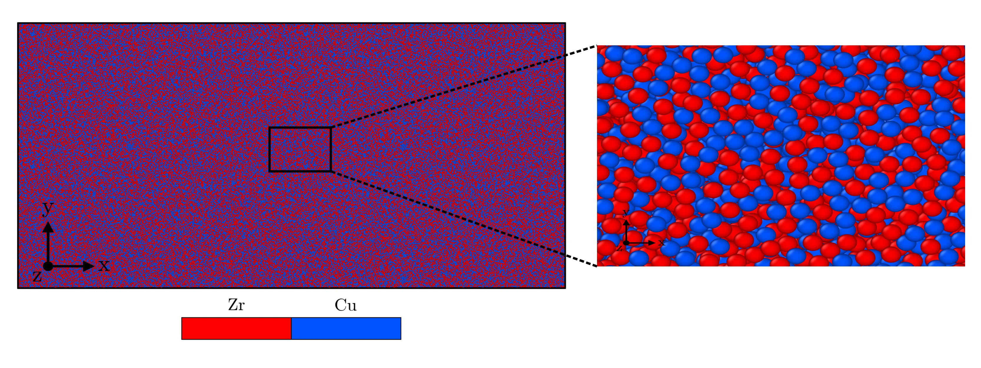
Figure 1: Visualization of the Cu₅₀Zr₅₀ MG system. Capture of the sample once its preparation had finished, including a small region that allows checking the amorphous state and the absence of crystallinity. This figure was obtained through the OVITO software [39].

The glass sample was prepared as follows: We start with a system of $145200$ Cu atoms with a FCC crystal structure, where 50% of these atoms are replaced by Zr atoms at random positions. Next, the system is heated from an initial temperature of 300 K to 2200 K for 2 ns (with an integration step $\Delta\tau=1$ fs), in the NPT ensemble, keeping the pressure constant at 0 GPa, thus obtaining a molten metal. The next step is to quench the sample quickly enough to avoid crystallization and obtain a glassy state system. For this, we reduced the temperature by 10 K followed by the procedure proposed by Wang et al. [40]. The $145200$ atoms in the glass are then replicated in the $x$ and $y$ direction, followed by a relaxation process in the NPT ensemble to remove all the problems caused by replication. Finally, we let the system evolves in the NVE ensemble for $100$ ps with a final minimization that ensures the interatomic forces are of the order of $10^{-4}$ eV$\cdot$Å^-1 and we thermalized it to $10$ K via Langevin thermostat, previous to the deformation process, following the methodology described by Sepúlveda-Macías et al. [41, 42].

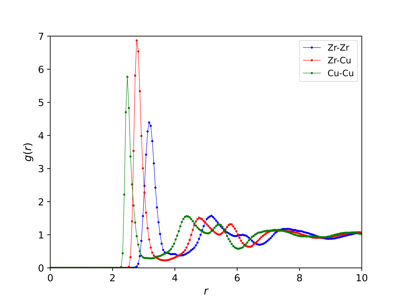
Figure 2: Partial radial distribution functions (RDF) for the MGs sample, computed at 10 K. Zr-Zr, Zr-Cu and Cu-Cu correlations are reviewed. The shape of these curves indicate a good agreement on the amorphous state of the system.

The resulting MG sample is presented in Figure 1. The partial radial distribution functions for the resulting Cu₅₀Zr₅₀ sample at 10 K are presented in Figure 2. As previously reported for this sample [37, 42], the location of the first peak and the split of second peak are fingerprints of an amorphous state. It is important to note that if we inspect closely the local structure of the sample, in Fig. 1, we noted the absence of any crystalline structure.

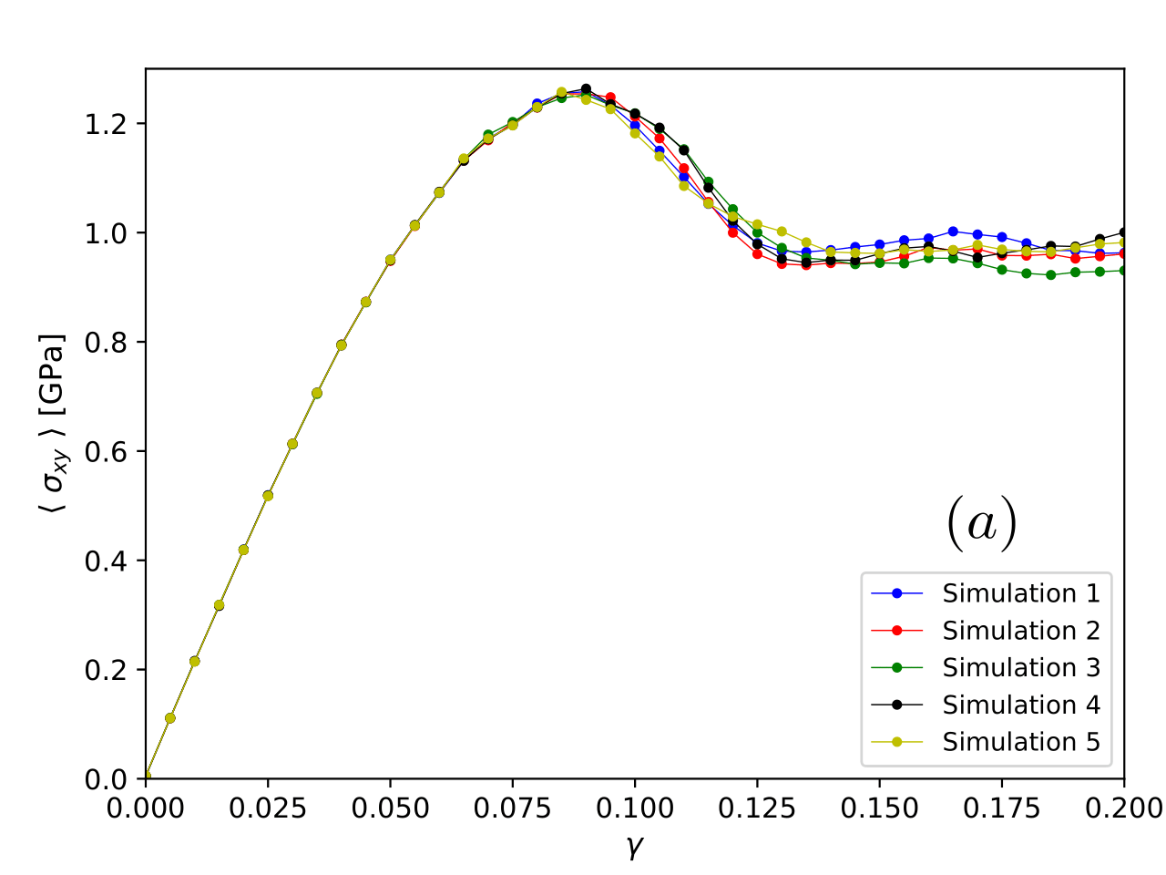
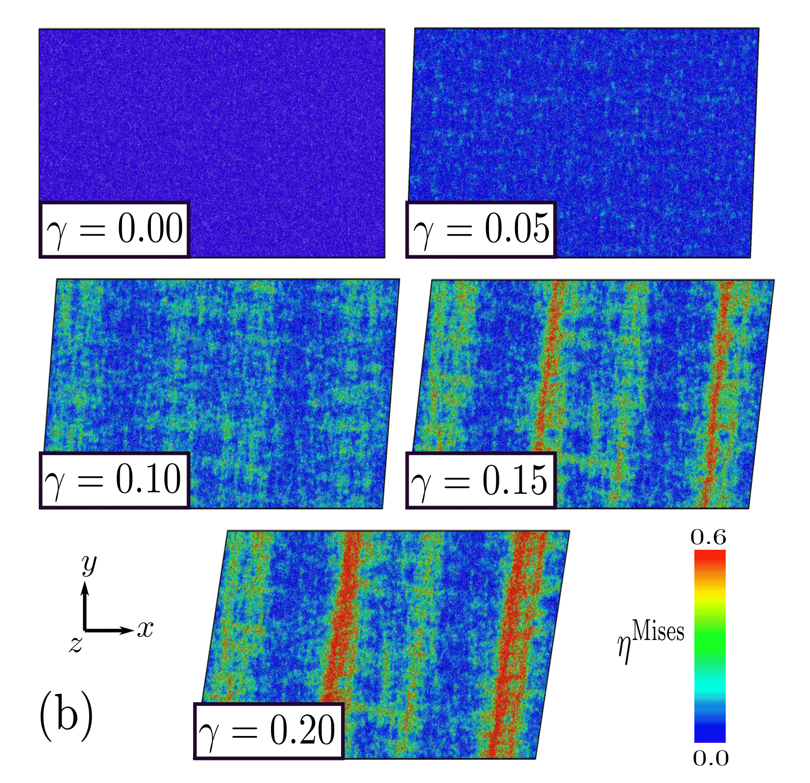
Figure 3: (a) Calculated stress-strain curves (S–S) for five simulations up to a global strain of $\gamma=0.20$. The stress $\langle\sigma_{xy}\rangle$ is calculated as the sum of the stress tensor component $\sigma_{xy}$ of all the atoms averaged over the cell volume. (b) Shear strain localization in the $xy$ plane, here the atoms are colored according to their local atomic shear strain (von Mises strain, $\eta^{\text{Mises}}$), which indicates the deformation degree. This measurements were done and monitored by the OVITO software [39].

Once the preparation of the MG was finished, we proceed to apply a shear deformation with a constant strain rate $\dot{\gamma}=5\times 10^{8}$ s^-1, up to a maximum strain of $\gamma=0.20$ (duration $0.4$ ns). We have obtained 5 different S–S curves for the elasto-plastic regime due to the thermalization. This process depends on an initial seed that generates the random force for the atoms in the theoretical model of the Langevin thermostat. In the 5 simulations, we have occupied different seeds, so that at the microscopic level each dynamic is different from one another, but at the macroscopic level, the material exhibits the same mechanical state once the plastic events take place.

Figure 3 shows the macroscopic stress-strain beaviour and the development of the shear band during the deformation process. In Figure 3-(a) the S–S curves for five independent simulations are presented. Each of them exhibit two well-defined regimes: up to $\gamma\sim 0.05$ the system responds elastically under shear stresses. Once this level of deformation is exceeded (yield strength), the sample begins to exhibit plastic and irreversible deformations, reaching its maximum load stress at $\gamma\sim 0.09$. After reaching the maximum stress, the system undergoes a stress drop followed by a stress plateau beyond $\gamma\sim 0.125$. At the atomic scale, it is possible to follow the evolution of the shear band using the local atomic shear strain, calculated by means of the von Mises strain $\eta^{\text{Mises}}$ and obtained through the strain tensor as proposed by Shimizu et al. [16]. This is shown in Figure 3-(b). As can be seen, during the elastic regime, up to $\gamma=0.05$, there is no occurrence of plastic events. Thereafter, there is an increase in plastic events that are homogeneously distributed throughout the specimen. These plastic events, or STZs, begin to coalesce and align to give way to the formation of the shear band. This phenomenon is clearly seen in Figure 3-(b) at global $\gamma=0.15$ where the red colored atoms mark the location of the SBs, after this strain state two SBs are fully developed with an approximate width of $\sim 75$ Å.

In the following section, we begin the statistical study of physical descriptors involved in the deformation process, descriptors that are necessary for the application of our CN model. We compute stress tensors, strain tensors, and strain gradient tensors for each of the atoms in the cell to develop the statistics analysis.

3 Statistical study of physical descriptors and plastic events

Plasticity in MGs is a topic that still lacks a solid theoretical framework. Until now, only models have been proposed that explain how the plastic deformation process works, among them, structural heterogeneities known as shear transformation zones and shear bands.

In this work, we seek to give a microscopic characterization of the elasto–plastic deformation, based on complex networks, that help us to describe the structural heterogeneities and the properties of the Cu₅₀Zr₅₀ as a function of external shear deformation. We track the mechanical behavior of the MG up to the point where the system reaches the mechanical failure. That is, the point at which the material fractures into two or more parts. For this purpose, we use a methodology based on CN where the atomic configurations of the system are mapped to a graph, thus obtaining an abstract representation of the material, via interacting edges and vertices. For the structure of these graphs, we have proposed a method that generates a growing network of vertices and edges as a function of strain. The evolution of these graphs, which is the result of mapping a time series of atomic configurations, results in a network with complex structural and dynamical properties. Details about the construction of the network are presented in the next section.

One of the main ingredients for the construction of the CN is the selection of a physical descriptor that we will use to designate the vertices. We know that the networks are only a mathematical instrument to represent a system of discrete elements, but to make sense of our problem, the physical information of the networks is contained in these descriptors. Some descriptors that we review are: the Shear Stress, the Shear Strain, the Volumetric Strain and the Non-Affine Displacement.

The Shear Stress or von Mises stress $\sigma^{\text{Mises}}$ is a quantity with units of GPa$\cdot\text{\AA}^{3}/V$ that we compute for each atom $\ell$ using its stress tensor through the expression

$$\sigma^{\text{Mises}}_{\ell}=\sqrt{\sigma_{xy}^{2}+\sigma_{xz}^{2}+\sigma_{yz}^{2}+\frac{(\sigma_{xx}-\sigma_{yy})^{2}+(\sigma_{xx}-\sigma_{zz})^{2}+(\sigma_{yy}-\sigma_{zz})^{2}}{6}}.$$ (1)

The Shear Strain or von Mises strain $\eta^{\text{Mises}}$ is a dimensionless quantity that we compute for each atom $\ell$ using its strain tensor through an expression equivalent to Shear Stress

$$\eta^{\text{Mises}}_{\ell}=\sqrt{\eta_{xy}^{2}+\eta_{xz}^{2}+\eta_{yz}^{2}+\frac{(\eta_{xx}-\eta_{yy})^{2}+(\eta_{xx}-\eta_{zz})^{2}+(\eta_{yy}-\eta_{zz})^{2}}{6}}.$$ (2)

The Volumetric Strain $\eta^{\text{Vol}}$ is a dimensionless quantity that we compute for each atom $\ell$ using the principal components of its strain tensor through the expression

$$\eta^{\text{Vol}}_{\ell}=\frac{1}{3}\Big{(}\eta_{xx}+\eta_{yy}+\eta_{zz}\Big{)}.$$ (3)

Finally, the Non-Affine Displacement $\mathscr{D}^{2}$ is a dimensionless quantity that corresponds to the least square error when trying to determine the best tensor transformation $\bar{\bar{F}}_{\ell}$ which maps from an initial undeformed configuration $\{{\bf d}_{j\ell}^{0}\}$, to a deformed configuration $\{{\bf d}_{j\ell}\}$. The index $j$ indicates the close neighbors to $\ell$, with $N^{0}_{\ell}$ the number of neighbors of atom $\ell$ at the reference configuration. This transformation $\bar{\bar{F}}$ is known as the deformation gradient tensor and is an element that allows us to determine the strain tensor. In conclusion, this descriptor would be

$$\mathscr{D}_{\ell}^{2}=\min\left\{\sum_{j\in N^{0}_{\ell}}\left|{\bf d}^{0}_{j\ell}\bar{\bar{F}}_{\ell}-{\bf d}_{j\ell}\right|^{2}\right\}.$$ (4)

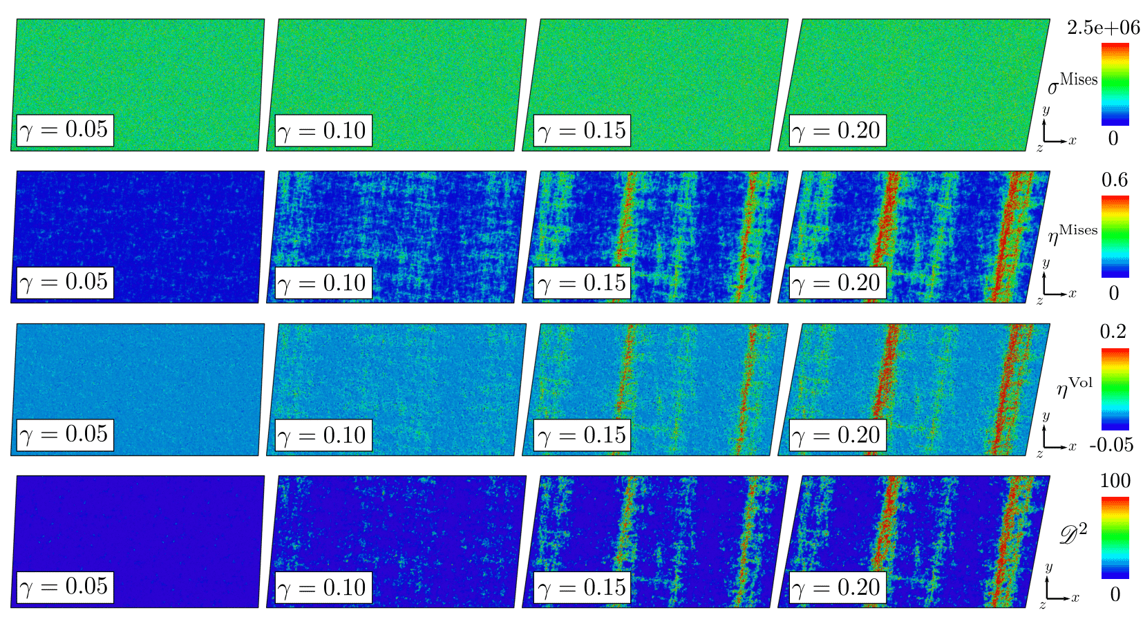
Figure 4: Spatial distribution, on the $xy$ plane, of descriptors $\alpha=\{\sigma^{\text{Mises}},\eta^{\text{Mises}},\eta^{\text{Vol}},\mathscr{D}^{2}\}$. For the deformation states $\gamma=\{0.05,0.10,0.15,0.20\}$, atoms are colored according to their descriptors values. When we compute the deformation gradient tensor $\bar{\bar{F}}$, we use a cutoff radius $r=5\text{ \AA}$ that defines the neighborhood $N_{\ell}^{0}$. The tensor $\bar{\bar{F}}$ allows to compute the strain tensor $\eta$ and all the descriptors.

A summary of the defined descriptors, applied to our amorphous sample, is presented in Figure 4. The maps in Figure (4) show the spatial distribution in the $xy$ plane of each descriptor at 4 different strain states.

These results indicate a good agreement with the phenomena of plastic deformation and shear band formation. For example, the spatial distribution of $\eta^{\text{Mises}}$, $\eta^{\text{Vol}}$, and $\mathscr{D}^{2}$ shows that the system will eventually undergoes fracture at the place where the SBs are formed. However, the spatial distribution of $\sigma^{\text{Mises}}$ is distributed homogeneously along the cell, regardless of whether the deformations are elastic or plastic. Although this result does not show any signal about deformation, perhaps its application to network construction can reveal some information about plasticity.

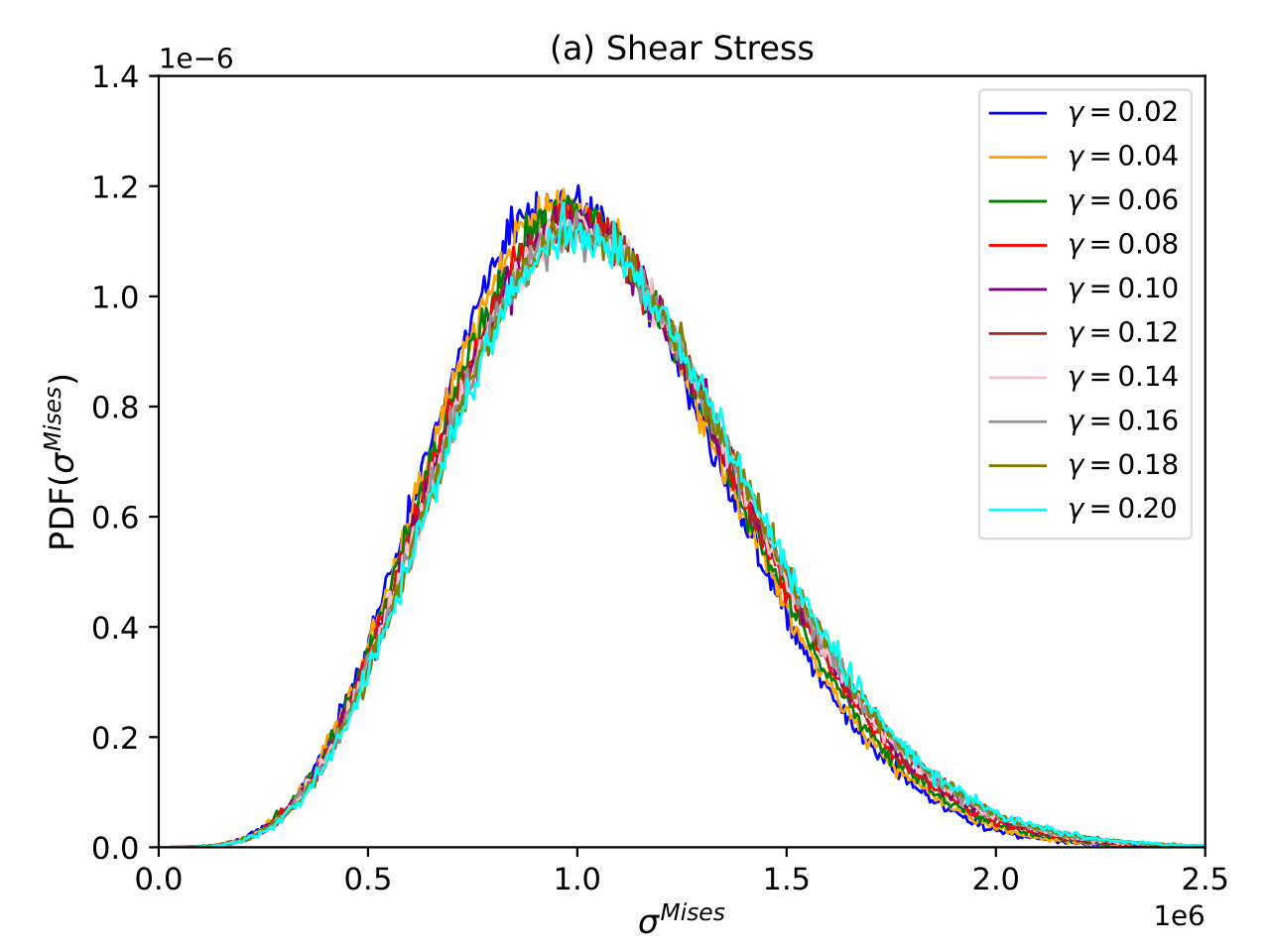
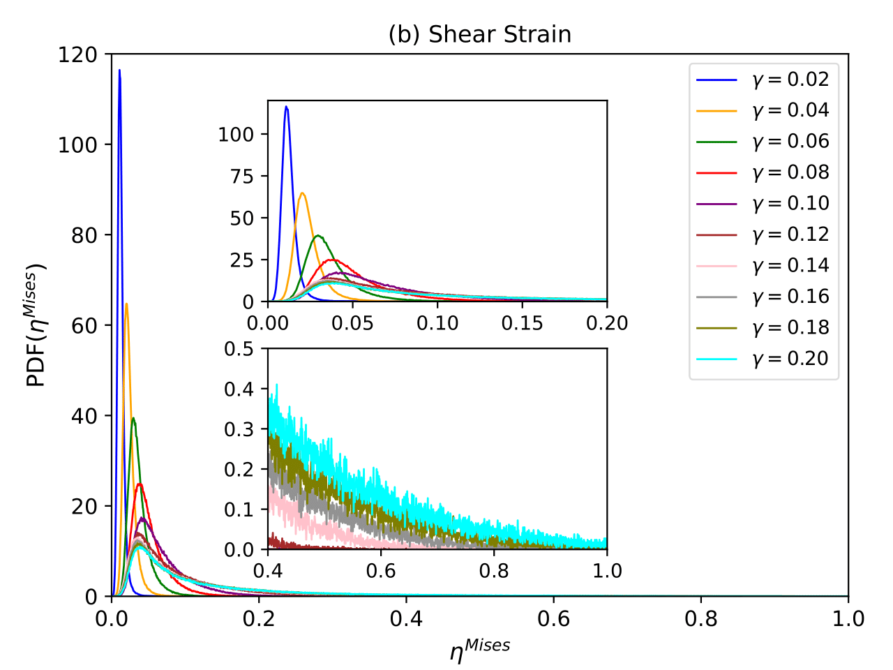
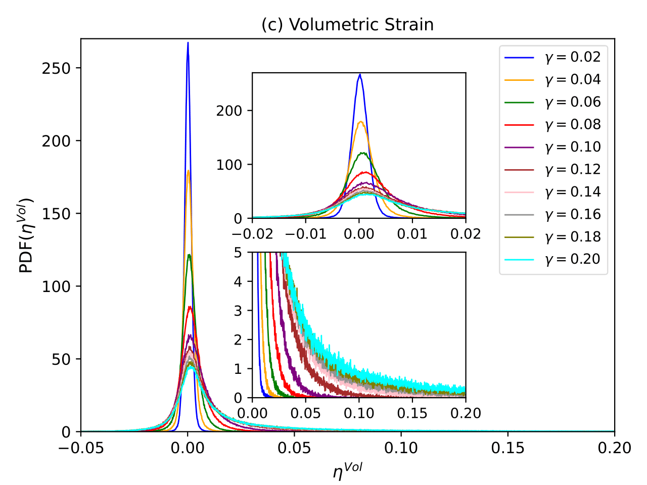
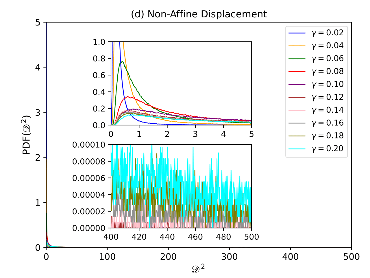
Figure 5: Probability density functions (value distributions) of (a) $\sigma^{\text{Mises}}$, (b) $\eta^{\text{Mises}}$, (c) $\eta^{\text{Vol}}$ and (d) $\mathscr{D}^{2}$, for different deformation states $\gamma$. The inset in (b), (c), and (d) are zoomed curves of the same respective distributions.

We have also computed the numerical distribution via probability density that is presented in Figure (5), which shows us how the values descriptors are distributed among each atom and for each deformation value. For the descriptor $\sigma^{\text{Mises}}$, we see that its values approximately fit a Gaussian distribution, independent of the deformation regime, unlike the others, which correlates with the homogeneous distribution seen in Figure (4). The $\eta^{\text{Mises}}$ distributions exhibit a dependency on the deformation state, where for elastic strain, $\eta^{\text{Mises}}\in(0,0.1)$ , and for plastic strains, $\eta^{\text{Mises}}\in(0,1)$. In this case, the standard deviation of the data increases as well as the average $\langle\eta^{\text{Mises}}\rangle$. On the other hand, the $\eta^{\text{Vol}}$ distributions show a Gaussian trend for every value of $\gamma$ under the restriction that as the strain increases, the standard deviation of the data increases, conserving their averages $\langle\eta^{\text{Vol}}\rangle$ around $0$, which makes physical sense since the system preserves its volume. Finally, the $\mathscr{D}^{2}$ distributions exhibit longer and longer tails as the strain increases. These types of distributions are interesting to study since they apparently have the form of a power law. Dozens of physical systems, such as earthquakes, solar flares, including material deformation [43], have reported power laws to some quantity, giving a better understanding of their behavior and complexity. It is interesting to study the tail of these $\mathscr{D}^{2}$ distributions.

In order to have a characterization of these distributions, we proceed to calculate the time series of the moments, providing us with statistical information on the data. From a statistical point of view, a distribution only provides probabilistic information about a random variable. However, one way to characterize the sample space is by computing properties such as the mean, variance, standard deviation, etc. These quantities can be calculated through the moments of a distribution. For this analysis, we work with the standardized moment $\hat{\mu}$. In this context, they are defined as

$$\hat{\mu}_{k}=\frac{\bar{\mu}_{k}}{\sigma^{k}}=\frac{\big{\langle}(\alpha-\mu)^{k}\big{\rangle}}{\sigma^{k}}=\frac{1}{\sigma^{k}}\int_{\alpha\in[a,b]}(\alpha-\mu)^{k}\rho(\alpha)d\alpha,$$ (5)

where $\alpha=\{\sigma^{\text{Mises}},\eta^{\text{Mises}},\sigma^{\text{Vol}},\mathscr{D}^{2}\}$ are the physical descriptors and $\rho(\alpha)$ are the probability density functions of the Figure (5). For the expression (5), we work with the central moment $\bar{\mu}_{k}$, centered on the average $\mu=\langle\alpha\rangle$, and normalized to the $k$th power of the standard deviation $\sigma=\sqrt{\langle(\alpha-\mu)^{2}\rangle}$. In Figure (6) we present the results obtained for the third and fourth standardized moments of each one of the descriptors. These results are basically the time series of the skewness and the kurtosis of the distributions. The first and second standardized moments are not calculated since it is clear that they are $0$ and $1$ respectively for the entire range of deformation.

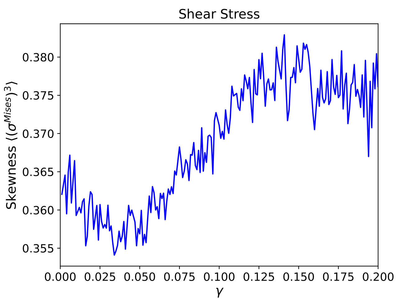
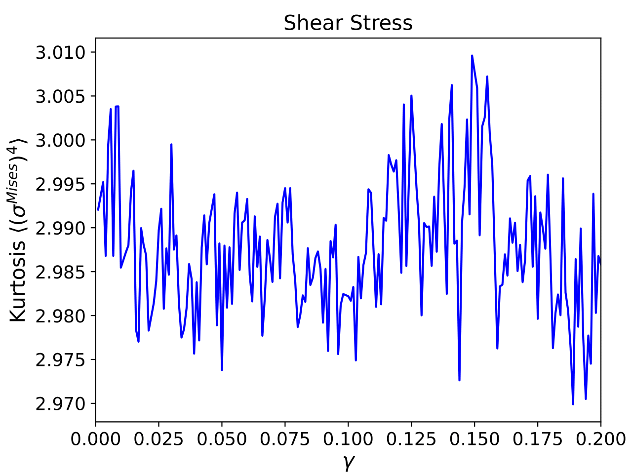
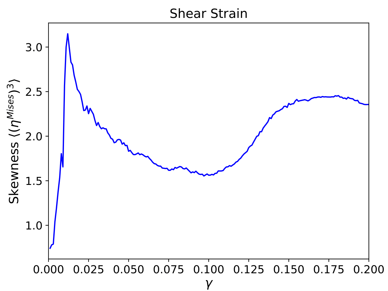
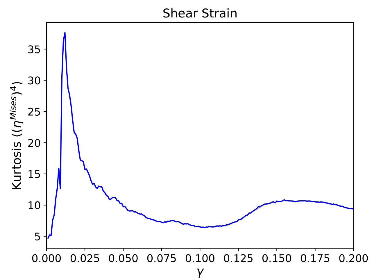
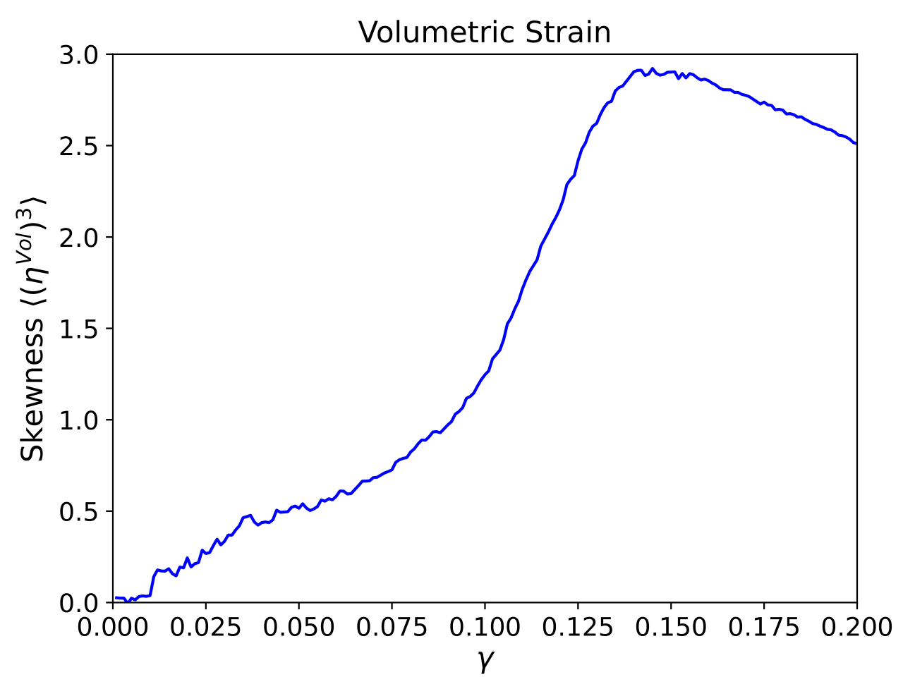
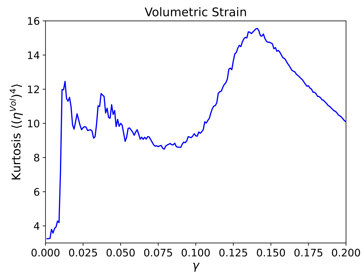
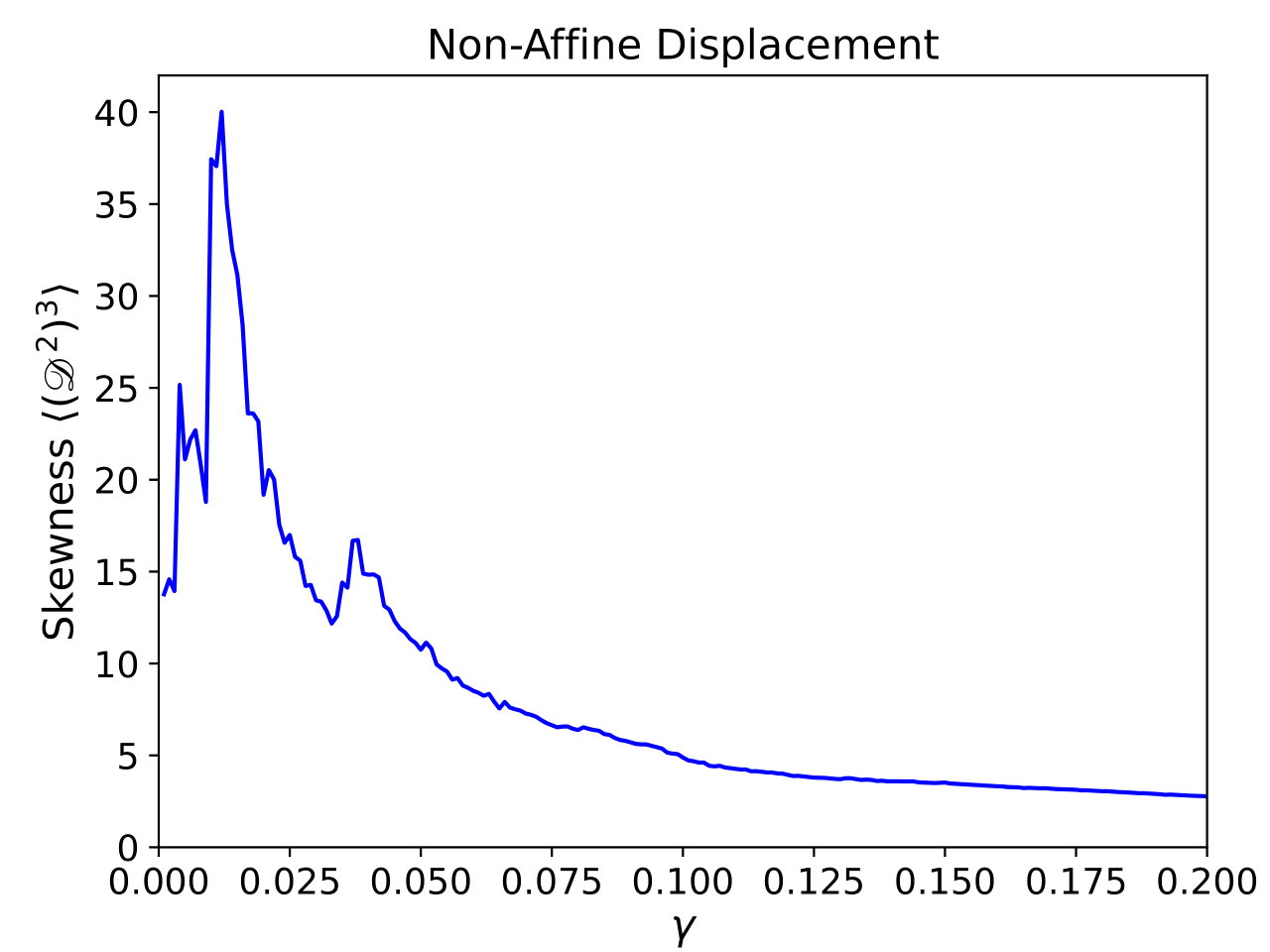
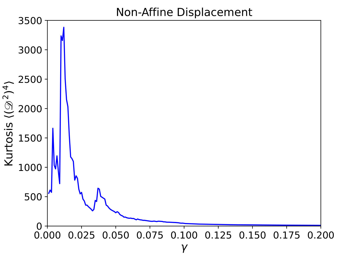
Figure 6: Third and fourth order standardized moments, from the distributions in Figure (5) as a function of strain and for descriptors $\alpha=\{\sigma^{\text{Mises}},\eta^{\text{Mises}},\eta^{\text{Vol}},\mathscr{D}^{2}\}$. These curves were calculated by means of the numerical integration that defines each moment (acoording to equation (5)) using the trapezoidal method.

The third-order moment (skewness) $\hat{\mu}_{3}$ is a value that quantifies the asymmetry of a distribution. The results presented in Figure (6) show that for all distributions there is always a positive skewness (heavy tails to the right) independent of the deformation state $\gamma$, but that is interesting to note are the variations that this property exhibits. For example, for $\sigma^{\text{Mises}}$ distributions, its skewness $\hat{\mu}_{3}\approx 0.3$, that is, it is almost a Gaussian with a slight asymmetry to the right. Interestingly, such asymmetry shows changes at points such as elasto-plastic transition and fracture of the material. That the distribution becomes more asymmetric to the right in the plastic regime and in the process of SBs formation, physically tells us that atoms with a high stress appear as a result of the dissipation of elastic energy, an interesting result, all from one statistical point of view. Now, the other descriptors show interesting variations, for example for the $\eta^{\text{Mises}}$ it decreases in the plastic regime, for the $\eta^{\text{Vol}}$ it increases drastically before the failure and for the $\mathscr{D}^{2}$ begins very asymmetric and as the strain increases, it attenuates.

On the other hand we have the fourth-order moment (kurtosis) $\hat{\mu}_{4}$. This statistical measure quantifies the degree of slope of the maximum and the tails of a distribution with respect to a Gaussian distribution. For our results in Figure (6), the kurtosis of each descriptor is positive for all strain values, indicating that there are atypical data in the tails and a steeper maximum. These atypical values are nothing more than the presence of highly stressed and/or deformed atoms. For the $\sigma^{\text{Mises}}$ it is relatively constant showing that the difference to a Gaussian does not change, and for the other descriptors, it indicates changes in relation to the deformation regime. This characterization is just another complementary result to our physical interpretation of the phenomena that occur in the material.

The next metric to study is a coefficient that allows to evaluate the level of inequality in a series of data. This metric is known as the Gini coefficient, a measure of statistical dispersion which is used in economics to study wealth inequality in a population. In our case, we are interested to compute how different (numerically) the data for each $\alpha$ descriptor is as a function of strain. To evaluate this coefficient, we need to calculate what is known as the Lorenz curve, which in this context would represent the fraction of the accumulated descriptor (equivalent to the fraction of wealth of a population) as a function of the fraction of accumulated atoms (equivalent to the population fraction).

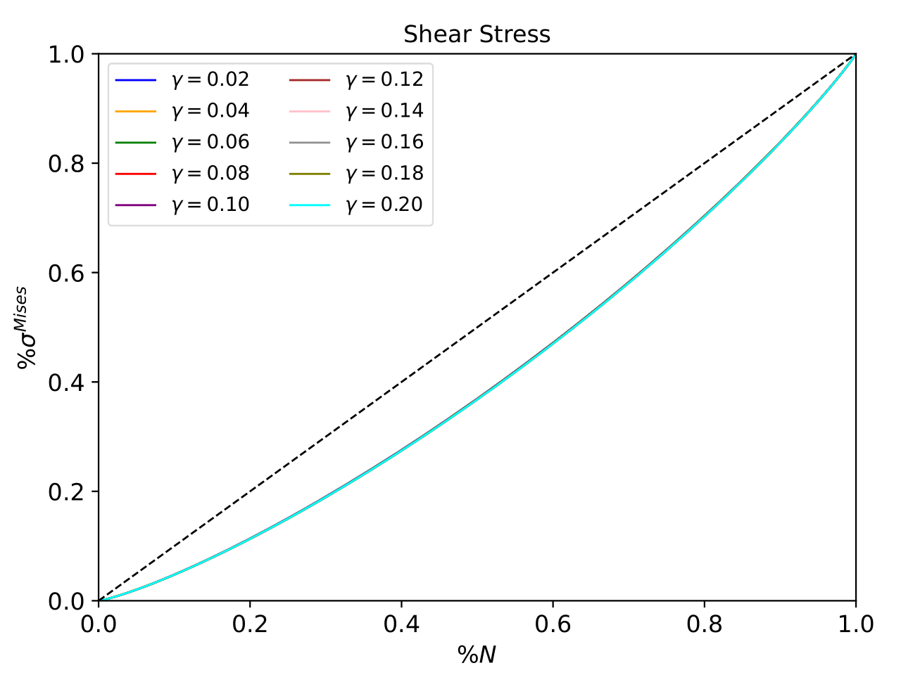
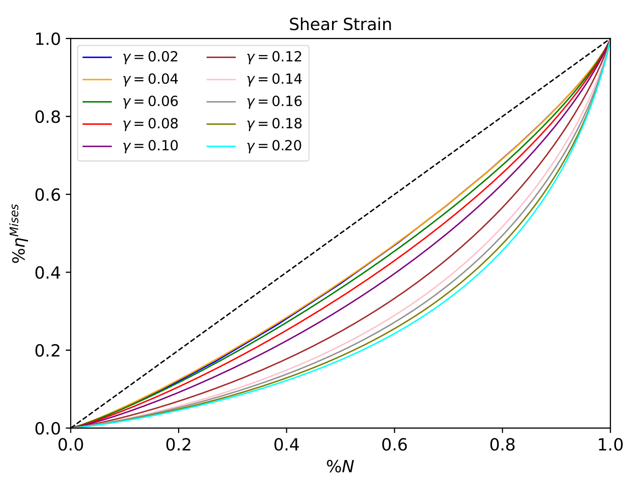
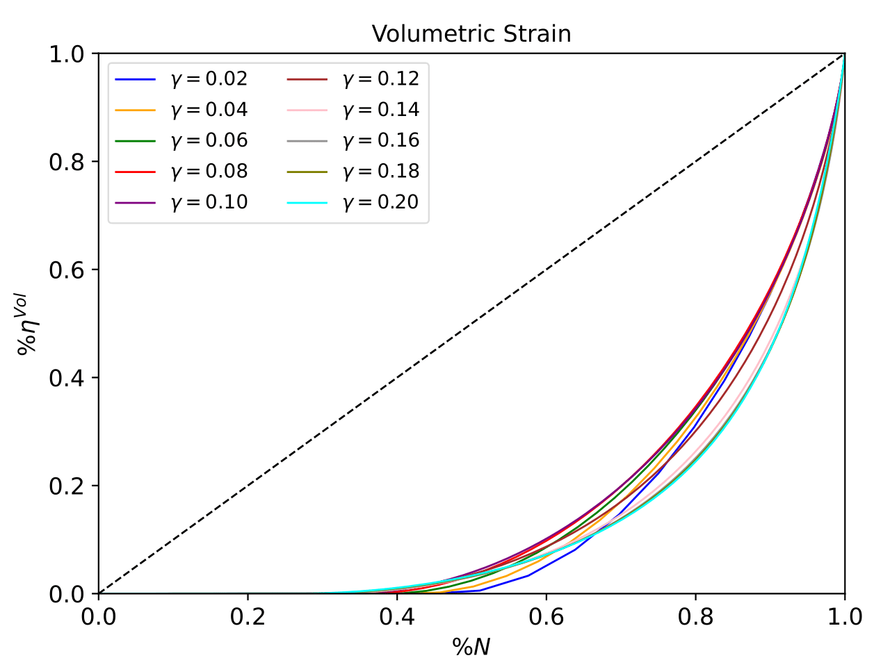
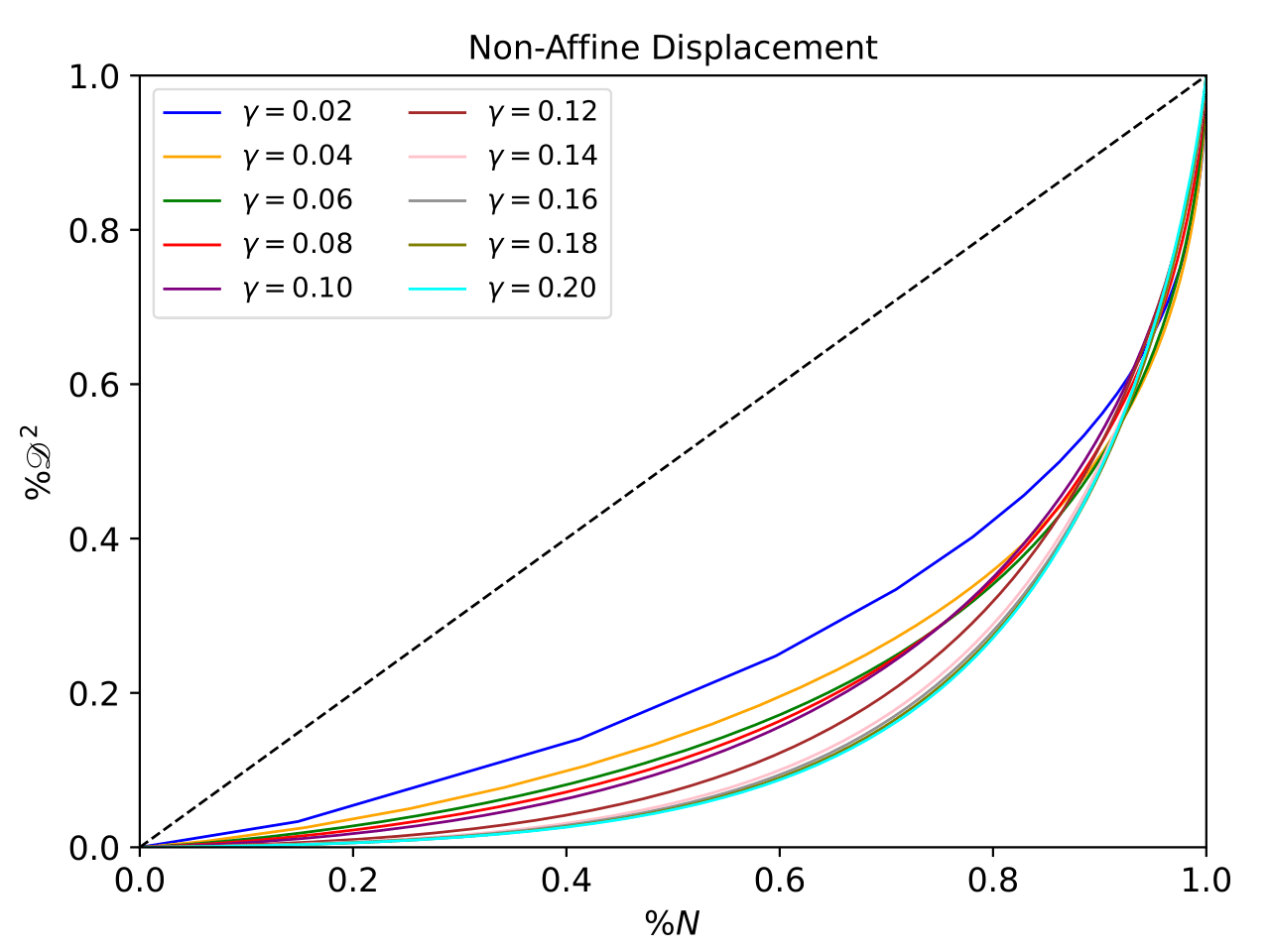
Figure 7: Lorenz curves of each of the distributions in the Figure (5) and for different strain values $\gamma$. The dashed line represents the maximum equality that can be had in a data distribution. This means that for the same percentage of the population there is the same percentage of wealth distributed among them. All the curves below the dashed line account for a degree of inequality that the system exhibits.

In economics or in whatever context it is applied, Lorenz curves are a visual representation of how unequal is the data distribution. These curves only take values between $0$ and $1$ since they evaluate the fraction of the total wealth that a fraction of the complete population owns. If the curve approximates to linear trend, the data distribution is more equality, since a given fraction of the population has the same amount of wealth. However, if the curve takes the form of a semi-parabola with a minimum at zero, it indicates that there is a degree of inequality in the data depending on the characteristics of said semi-parabola. Reviewing Figure (7), we see that the Lorenz curves of the $\sigma^{\text{Mises}}$ approximate a linear equation independent of the deformation regime, that is , the data is distributed almost equally over the system. The above makes sense since the $\sigma^{\text{Mises}}$ is distributed homogeneously according to the map in Figure (4). On the other hand, the Lorenz curves of the $\eta^{\text{Mises}}$ and the $\mathscr{D}^{2}$ take the form of a semi-parabola increasing its convexity as the strain increases. At greater convexity, greater the level of inequality. In the case of $\eta^{\text{Vol}}$, at least 40% of the population of atoms presents a descriptor value that is very different from the average, increasing the inequality considerably. Although the probability density of $\sigma^{\text{Mises}}$ and $\eta^{\text{Vol}}$ look like a Gaussian, they will not necessarily have the same properties.

Now that we have an idea of how unequal is the distribution of each descriptor via Lorenz curves, we proceed to quantify said inequality by calculating the Gini coefficient, which can be calculated by two different ways:

$$G=\frac{A}{A+B}=\bigg{|}1-\sum_{k=1}^{n-1}(X_{k+1}-X_{k})(Y_{k+1}+Y_{k})\bigg{|},$$

where $A$ is the area between the line of perfect equality and the Lorenz curve, and $B$ is the area under the Lorenz curve. Since the area under the perfect equality curve is $0.5$, it is clear to see that $A+B=0.5$, so an alternative expression for this coefficient would be $G=1-2B$. On the other hand, we have Brown’s formula, an expression that uses the cumulative proportion of the population variable $X_{k}$ and the cumulative proportion of the descriptor variable $Y_{k}$, to quantify this coefficient. In order to have a more complete study, both results are presented for the entire time series of the Gini coefficient of the all descriptors.

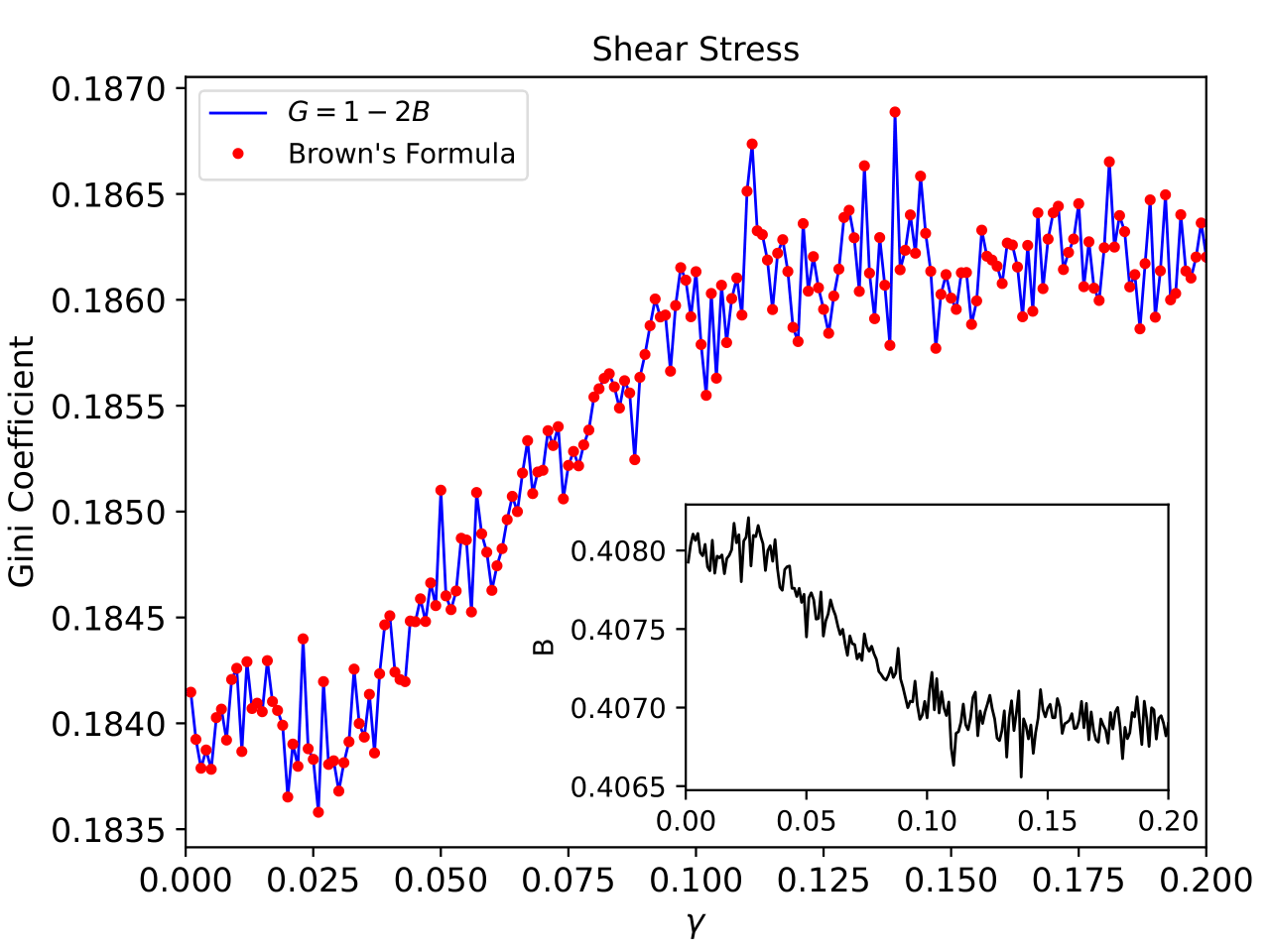
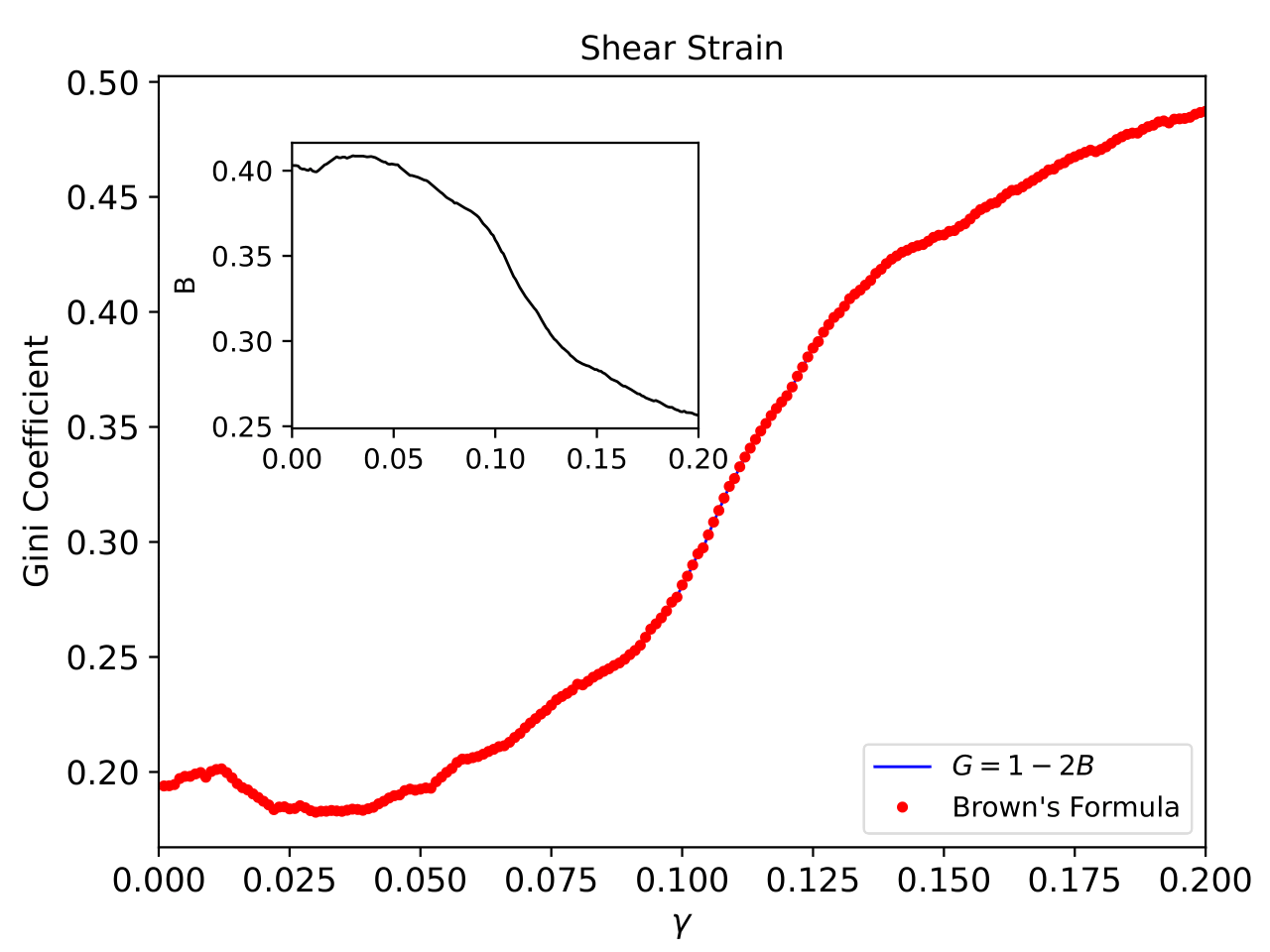
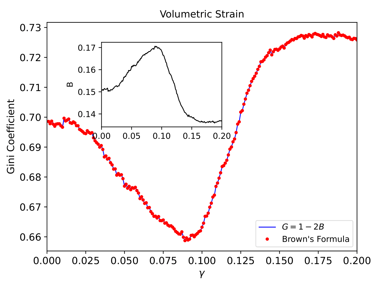
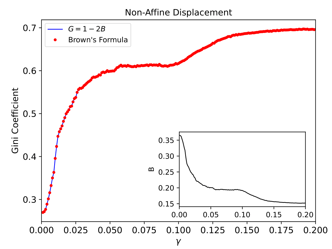
Figure 8: Gini coefficient as a function of strain for each of the distributions in Figure (5), computed using the area formula (numerical integration via the trapezoidal method) and Brown’s formula. The area under the Lorenz curves as a function of strain is included in the inset. All the curves show a change as a function of the deformation state of the system: elastic regime ($\gamma<0.45$), plastic regime ($0.45<\gamma<0.95$) and plastic creep ($0.95<\gamma$).

The values that the Gini coefficient can take are between $0$ and $1$, where $0$ represents perfect equality and $1$ maximum inequality. In relation to the analysis made on the Lorenz curves and the results obtained in Figure (8), we see that the Gini coefficient gives us better precision to evaluate inequalities. For example, in the case of $\sigma^{\text{Mises}}$, despite the fact that its Lorenz curves reflected a relative equality in the data distribution, the Gini coefficient shows how this relative equality is slowly lost when plastic deformations begin, saturating until the SB formation process. Although the range of values that this coefficient takes for this descriptor is $G\sim 0.18$, it is interesting to note that information that is not possible to see with all the previous results. On the other hand, for the descriptors $\eta^{\text{Mises}}$ and $\mathscr{D}^{2}$, their Gini coefficient increases as a function of strain, registering variations up to $\Delta G\sim 0.3$ for the $\eta^{\text{Mises}}$ data and $\Delta G\sim 0.45$ for the $\mathscr{D}^{2}$ data through the deformation process. This positive variation indicates that the data for both descriptors are distributed with less equality, which shows that there are atoms, or clusters of atoms that acquire even more atypical values. For the $\eta^{\text{Mises}}$, the variations of inequality are recorded when the plastic deformations $(\gamma>0.5)$ begin, and when the SB is located $(\gamma\sim 0.95)$, unlike of the $\mathscr{D}^{2}$, that such important variations are registered for the elastic deformations $(\gamma<0.5)$ and when the SB is located. This result is an elegant way of verifying that the different mechanical states that the system adopts under an external stress have multiple properties. On the one hand, the Shear Strain is relatively egalitarian in the elastic regime, until when the plastic regime begins, select groups of atoms (apparently random), take a large part of the Shear Strain, evidenced in the formation of a SB in Figure (4). And on the other hand, the Non-Affine Displacement evidences a growing inequality due to the underlying physical phenomena, showing that a simple result of a minimization can reveal macroscopic properties.

All the statistical analysis that we have presented in this section has allowed us to characterize the deformation process in a microscopic way, identifying the different mechanical states that the system adopts, the plastic events that are identified as the STZs and that give rise to the SBs, in order to finally, have a macroscopic characterization of the material. In the following section we begin the presentation of our methodology based on CNs for our research.

4 Complex network model

In general, a CN is a set of vertices and edges connecting them that can be defined to represent a given physical system or process, by means of a suitable definition for the vertices and edges. Such definitions depend on the specific problem that we intend to model. As previously mentioned, CNs approaches have been successfully used to study localized energy release processes such as seisms [31, 33, 34, 44], solar flares [22], and sunspots [35]. In these works, the vertices correspond to a spatial region where an event occurs (seism, flare and/or sunspot), and the connections are given by a temporal sequence. For a seismic catalog, only one event occurs at a time, so the connections are between consecutive seisms. Thus, the spatial information is contained in the vertices, and the temporal evolution in the edges of the network. In the reference [35], the authors follow a similar strategy, except that the vertices were defined using a certain threshold for the magnetic field, and defining them as pixels in a solar magnetogram. The resulting network is a representation of the spatiotemporal evolution of sunspots. All these works have shown that the topological measures of the resulting network contain information about the underlying physical processes. Our purpose then is to study whether a similar technique can be used to study the deformation process in MG sample.

In this study, we are interested in characterizing the atomic events that originate in the MG during a shear deformation. For this, we have used only three descriptors, which are $\alpha=\{\sigma^{\text{Mises}},\eta^{\text{Mises}},\mathscr{D}^{2}\}$. Then, following the references [33, 34, 35], we have defined the vertices as the atoms that satisfy the following conditions:

$$\sigma_{0}^{\text{Mises}} < \sigma^{\text{Mises}}_{\ell s}$$ (6)

$$\eta_{0}^{\text{Mises}} < \eta^{\text{Mises}}_{\ell s}$$ (7)

$$\mathscr{D}_{0}^{2} < \mathscr{D}_{\ell s}^{2}$$ (8)

where $\alpha_{0}=\{\sigma_{0}^{\text{Mises}},\eta_{0}^{\text{Mises}},\mathscr{D}_{0}^{2}\}$ are defined as the vertices selector thresholds. On the other hand, the $\alpha_{\ell s}=\{\sigma_{\ell s}^{\text{Mises}},\eta_{\ell s}^{\text{Mises}},\mathscr{D}_{\ell s}^{2}\}$ are the values that each descriptor takes for the atoms $\ell$, monitored at time $t_{s}$ of the simulation. Independently, if any of the above inequalities is satisfied, the atom $\ell$ at time $t_{s}$ becomes a vertex of the network. Each descriptor is worked independently, this means that if we are working with $\sigma^{\text{Mises}}$ descriptor, it is enough that (6) is fulfilled to generate the vertices. If we are working with $\eta^{\text{Mises}}$, it is enough that (7) is fulfilled and so on with the other. It is important to mention that the choice of these thresholds determines the density of vertices that each CN will have.

After having classified the atoms as vertices using any of the descriptors, we proceed to establish the edges between them. For this particular model, the edges are established between consecutive times of the simulation, that is, all the vertices of the time $t_{s}$ are connected by an edge with all the vertices of the time $t_{s+1}$. This is a similar protocol used for solar magnetograms [35]. Note that this allows one atom to be connected to any other, as long as (6-8) is satisfied at consecutive times. However, although edges do not imply causality, one could argue that the connections between atoms are more meaningful if they are closer, given the locality of interactions leading to deformation. Thus, we add a locality condition, which states that a connection between two vertices only occurs if it is satisfied:

$$\sqrt{(x_{\ell}-x_{m})^{2}+(y_{\ell}-y_{m})^{2}+(z_{\ell}-z_{m})^{2}}\leq R_{0}.$$ (9)

Here, $\textbf{r}_{\ell}=(x_{\ell},y_{\ell},z_{\ell})$ and $\textbf{r}_{m}=(x_{m},y_{m},z_{m})$ are the position vectors of the vertices $\ell,m$ respectively, and $R_{0}$ is the value of cutoff radius that defines the neighborhood where connections are allowed for vertex $\ell$.

Other rules that satisfy the connections in our model and that are consistent with previous work [33, 34, 35] are:

1. The graphs are undirected, i.e., the edges have no direction of connection.

2. Vertices at the initial instant $t_{0}$ have no edges. The first edges appear at the next time.

3. Suppose we are working with the descriptor $\sigma^{\text{Mises}}$. A vertex at $t_{s}$ will remain in the network along the simulation even if at later times the condition $\sigma_{0}^{\text{Mises}}<\sigma^{\text{Mises}}_{\ell p}$ is not satisfied with $t_{s}<t_{p}$. The only consequence of this is that said vertex will not receive connections in $t_{p}$. The above also applies to the other descriptors.

4. Multi-edge and self-connections are not allowed.

5. The locality condition (9) respects periodic boundary conditions, i.e., it is possible for two vertices to be connected even though they are at opposite ends of the cell.

In this model we propose, each atomic configuration of the MG is mapped to a set of vertices, providing instantaneous information about the system. The vertices are then connected as the simulation progresses. When this is carried out during a certain time interval, the resulting network is expected to contain relevant information about microscopic events via computation of topological metrics.

Interested in the study of plasticity and microscopic events generated in MG, we have developed a shear deformation up to $20$% with a strain rate of $\dot{\gamma}=5\times 10^{8}$ s ^-1. This implies, that we must simulate for $0.4$ ns (400,000 time steps). Every $2$ ps (2000 time steps), we monitor the positions, velocities, and tensors associated with the deformation of all the atoms, to update the growth of the network. This implies that the times in which the network will receive new vertices and edges are $t_{s}=\{0,2,4,6,...,400\}$ ps with $s=\{0,1,2,...,200\}$ and with its corresponding state/strain value $\gamma_{s}=\{0,0.001,0.002,...0.2\}$.

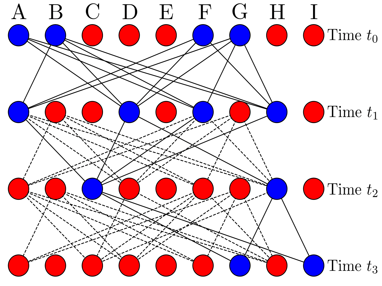
Figure 9: Representation of the CN model that we propose. (a) Diagram that illustrates the protocol to set the edges between pairs of vertices while the MD performs shear deformation. Four consecutive times and a nine-atoms system have been considered. The blue atoms are identified as the network vertices and the red ones are the atoms that do not satisfy the threshold condition. Vertices at time $t_{s}$ are connected to all vertices at time $t_{s+1}$. The graph grows in time, so the number of edges of each vertice changes. Solid and dashed lines represent new and past edges, respectively. For this particular case, we have selected a neighborhood $R_{0}$ large enough to allow all connections between the vertices from time $t_{s}$ to $t_{s+1}$.

Figure (9) illustrates the network construction process, showing how the edges connect pairs of vertices at consecutive times of the simulation. In particular and without loss of generality, we have considered the first four times (6 ps equals 6000 time steps). Initially, there are only vertices, always preserving the previous connections through the dashed lines.

4.0.1 Topological metrics

To study the dynamical and structural properties of CN, we compute topological metrics such as degree, clustering coefficient, and centrality, which provide a characterization of the network as the strain increases.

The degree ($k_{\ell}$) is the number of connections of the vertex indexed by $\ell$. In our model we work with undirected networks, therefore, we do not have the concept of incoming and outgoing degree. Thus, the average degree $\langle k\rangle$ of the network is defined as:

$$\langle k\rangle_{\gamma_{s}}=\frac{1}{n(\nu_{s})}\sum_{\ell\in\nu_{s}}^{n(\nu_{s})}k_{\ell},$$ (10)

where $\nu_{s}$ is the set of vertices, $n(\nu_{s})$ is the number of vertices, $k_{\ell}$ is the degree, which is computed by adding all the edges that the vertex $\ell$ has in $\nu_{s}$, and $\langle k\rangle_{\gamma_{s}}$ is the average degree for a strain $\gamma_{s}$ at time $t_{s}$.

Based on this metric, one way to obtain a more complete characterization of the network is by computing the degree probability distribution. This distribution contains information about the nature of the network and the underlying physical processes involved in its construction [20], being able to distinguish between purely random processes if the distribution is Poisson, and processes under preferential attachment growth, if the distribution is a power law [45].

Another useful metric is the clustering coefficient [20, 21, 46], which quantifies the number of connections between the neighbors of a given vertex. Thus, this provides information on the density of connections in the network. If all the neighbors of a vertex $\ell$ are connected to each other, then the clustering coefficient of $\ell$ takes the maximum value $1$, whereas if they are not connected, the clustering coefficient would be $0$. For undirected networks, we compute the clustering coefficient of vertex $\ell$ at time $t_{s}$ and its average over the network as:

$$C_{\ell s}=\sum_{j,k}\frac{2e_{jk}}{k_{\ell}(k_{\ell}-1)}\quad\;\;\;\;\text{and}\;\;\;\quad\langle C\rangle_{\gamma_{s}}=\frac{1}{n(\nu_{s})}\sum_{\ell\in\nu_{s}}^{n(\nu_{s})}C_{\ell s},$$ (11)

where the indices $j$ and $k$ denote the neighbors of vertex $\ell$. The terms $e_{jk}$ are the coefficients of the adjacency matrix of the network and can take the values $1$ or $0$, indicating if the neighbors $j$ and $k$ are connected or disconnected respectively. The average clustering coefficient $\langle C\rangle_{\gamma_{s}}$ can provide information about the global structure, existence of communities, connectivity and how robust or vulnerable is a CN.

To study the centrality of a graph and evaluate the importance of the vertices, metrics such as betweeness centrality, closeness centrality, among others, are used. Each of them quantifies the importance of the vertices in a different way, helping to give different interpretations to the network structure. For our study we use betweeness centrality, a metric that measures the importance of a vertex in terms of how many times it bridges along geodesics between other vertices. It is defined as the sum of the fraction of all pairs of shortest paths through which a vertex $\ell$ passes. Thus,

$$C^{B}_{\ell s}=\frac{2}{\big{(}n(\nu_{s})-1\big{)}\big{(}n(\nu_{s})-2\big{)}}\sum_{i,j\in\nu_{s}}\frac{\sigma(i,j|\ell)}{\sigma(i,j)}\quad\;\;\;\;\text{and}\;\;\;\quad\langle C^{B}\rangle_{\gamma_{s}}=\frac{1}{n(\nu_{s})}\sum_{\ell\in\nu_{s}}^{n(\nu_{s})}C^{B}_{\ell s},$$ (12)

where $\sigma(i,j)$ is the number of shortest paths joining the vertices $i$ and $j$, and $\sigma(i,j|\ell)$ is the number of shortest paths through which the vertex $\ell$ passes and that join the vertices $i$ and $j$. If $i=j$, then $\sigma(i,j)=1$, and if $\ell=\{i,j\}$ then $\sigma(i,j|\ell)=0$. The term that precedes the sum is the factor that normalizes the metric, in our case, for an undirected graph. The average betweenness centrality $\langle C^{B}\rangle_{\gamma_{s}}$ is a very useful metric to have information about the entire network. For example, it is a good indicator of vulnerability and resilience. Vulnerability is understood as a network that is sensitive to being disconnected if a vertex with high betweenness is eliminated, while a resilient network is a more robust network, i.e., it preserves its properties even if it loses important vertices. Also, the distribution of this metric allows us to analyze whether there are hierarchies in CNs.

The other centrality measure we use is closeness centrality, a metric that measures the average distance from a given vertex to all other vertices in terms of geodesics. The closeness is defined as the multiplicative inverse of the distance between two vertices. Mathematically

$$C^{C}_{\ell s}=\frac{n(\nu_{s})-1}{\sum_{i\in\nu_{s}}d(\ell,i)}\quad\;\;\;\;\text{and}\;\;\;\quad\langle C^{C}\rangle_{\gamma_{s}}=\frac{1}{n(\nu_{s})}\sum_{\ell\in\nu_{s}}^{n(\nu_{s})}C^{C}_{\ell s},$$ (13)

where $d(\ell,i)$ is the geodesic distance between vertices $\ell$ and $i$, and $n(\nu_{s})-1$ are all possible connections that vertex $\ell$ can have and that is used to normalize the metric.

Graph theory provides a wide variety of metrics and topological measures to characterize the structure of networks. In this study we use the degree, the clustering coefficient and centrality to characterize the resulting networks from the mapping of each atomic configuration product of the deformation of the MG. The objective is to carry out a microscopic analysis of the deformation, and to observe the macroscopic physical phenomena by means our CN methodology.

5 Topological metric calculations

We start the construction of the CN by randomly selecting different values for the vertex selection threshold for the three descriptors. We remember that the selection of these thresholds cannot be arbitrary since the density of vertices of the graphs depends precisely on this value. For very low thresholds, the density of vertices increases, making the numerical computation of CN untenable, but for higher thresholds, the density of vertices decreases, and therefore we will have unpopulated networks for the study. Another parameter that we must select is the cutoff radius that defines the neighborhood where connections are allowed for a vertex. The selection of this parameter influences the density of connections that the CN will have, so and in view of the dimensions of the simulation cell, for our study we have selected the radii $R_{0}=\{10,20,30,40,50\}$ Å.

Before proceeding with the construction of the networks and the calculation of the metrics, we present the data of all the thresholds that we have used to apply our methodology. The objective is to carry out a preliminary analysis to decide which threshold(s) is(are) most suitable for the study.

Shear Stress [GPa$\cdot\text{A}^{3}/V$]					Shear Strain
$[\sigma_{0}^{\text{Mises}}]_{1}$	$2.25\times 10^{6}$	$[\sigma_{0}^{\text{Mises}}]_{11}$	$2.56\times 10^{6}$		$[\eta_{0}^{\text{Mises}}]_{1}$	$0.5649$	$[\eta_{0}^{\text{Mises}}]_{11}$	$0.7524$
$[\sigma_{0}^{\text{Mises}}]_{2}$	$2.28\times 10^{6}$	$[\sigma_{0}^{\text{Mises}}]_{12}$	$2.59\times 10^{6}$		$[\eta_{0}^{\text{Mises}}]_{2}$	$0.5837$	$[\eta_{0}^{\text{Mises}}]_{12}$	$0.7711$
$[\sigma_{0}^{\text{Mises}}]_{3}$	$2.31\times 10^{6}$	$[\sigma_{0}^{\text{Mises}}]_{13}$	$2.62\times 10^{6}$		$[\eta_{0}^{\text{Mises}}]_{3}$	$0.6024$	$[\eta_{0}^{\text{Mises}}]_{13}$	$0.7899$
$[\sigma_{0}^{\text{Mises}}]_{4}$	$2.34\times 10^{6}$	$[\sigma_{0}^{\text{Mises}}]_{14}$	$2.65\times 10^{6}$		$[\eta_{0}^{\text{Mises}}]_{4}$	$0.6212$	$[\eta_{0}^{\text{Mises}}]_{14}$	$0.8086$
$[\sigma_{0}^{\text{Mises}}]_{5}$	$2.37\times 10^{6}$	$[\sigma_{0}^{\text{Mises}}]_{15}$	$2.69\times 10^{6}$		$[\eta_{0}^{\text{Mises}}]_{5}$	$0.6399$	$[\eta_{0}^{\text{Mises}}]_{15}$	$0.8273$
$[\sigma_{0}^{\text{Mises}}]_{6}$	$2.40\times 10^{6}$	$[\sigma_{0}^{\text{Mises}}]_{16}$	$2.72\times 10^{6}$		$[\eta_{0}^{\text{Mises}}]_{6}$	$0.6587$	$[\eta_{0}^{\text{Mises}}]_{16}$	$0.8461$
$[\sigma_{0}^{\text{Mises}}]_{7}$	$2.43\times 10^{6}$	$[\sigma_{0}^{\text{Mises}}]_{17}$	$2.75\times 10^{6}$		$[\eta_{0}^{\text{Mises}}]_{7}$	$0.6774$	$[\eta_{0}^{\text{Mises}}]_{17}$	$0.8648$
$[\sigma_{0}^{\text{Mises}}]_{8}$	$2.47\times 10^{6}$	$[\sigma_{0}^{\text{Mises}}]_{18}$	$2.78\times 10^{6}$		$[\eta_{0}^{\text{Mises}}]_{8}$	$0.6961$	$[\eta_{0}^{\text{Mises}}]_{18}$	$0.8836$
$[\sigma_{0}^{\text{Mises}}]_{9}$	$2.50\times 10^{6}$	$[\sigma_{0}^{\text{Mises}}]_{19}$	$2.81\times 10^{6}$		$[\eta_{0}^{\text{Mises}}]_{9}$	$0.7149$	$[\eta_{0}^{\text{Mises}}]_{19}$	$0.9023$
$[\sigma_{0}^{\text{Mises}}]_{10}$	$2.53\times 10^{6}$	$[\sigma_{0}^{\text{Mises}}]_{20}$	$2.84\times 10^{6}$		$[\eta_{0}^{\text{Mises}}]_{10}$	$0.7336$	$[\eta_{0}^{\text{Mises}}]_{20}$	$0.9211$

Non-Affine Displacement
$[\mathscr{D}^{2}_{0}]_{1}$	$632$	$[\mathscr{D}^{2}_{0}]_{6}$	$791$	$[\mathscr{D}^{2}_{0}]_{11}$	$949$	$[\mathscr{D}^{2}_{0}]_{16}$	$1107$
$[\mathscr{D}^{2}_{0}]_{2}$	$664$	$[\mathscr{D}^{2}_{0}]_{7}$	$822$	$[\mathscr{D}^{2}_{0}]_{12}$	$980$	$[\mathscr{D}^{2}_{0}]_{17}$	$1139$
$[\mathscr{D}^{2}_{0}]_{3}$	$696$	$[\mathscr{D}^{2}_{0}]_{8}$	$854$	$[\mathscr{D}^{2}_{0}]_{13}$	$1012$	$[\mathscr{D}^{2}_{0}]_{18}$	$1170$
$[\mathscr{D}^{2}_{0}]_{4}$	$727$	$[\mathscr{D}^{2}_{0}]_{9}$	$885$	$[\mathscr{D}^{2}_{0}]_{14}$	$1044$	$[\mathscr{D}^{2}_{0}]_{19}$	$1202$
$[\mathscr{D}^{2}_{0}]_{5}$	$759$	$[\mathscr{D}^{2}_{0}]_{10}$	$917$	$[\mathscr{D}^{2}_{0}]_{15}$	$1075$	$[\mathscr{D}^{2}_{0}]_{20}$	$1234$

Table 1: Thresholds values that map an atom to a vertex for the descriptors $\alpha=\{\sigma^{\text{Mises}},\eta^{\text{Mises}},\mathscr{D}^{2}\}$. 20 thresholds for each descriptor are chosen and used for the construction of the networks.

The previous study consisted in building the CN using each of the thresholds of the Table (1) and the set of cutoff radii $R_{0}$. The parameters set $(\alpha,[\alpha_{0}]_{i},R_{0})$, where $[\alpha_{0}]_{i}=\Big{\{}[\sigma_{0}^{\text{Mises}}],[\eta_{0}^{\text{Mises}}],[\mathscr{D}^{2}_{0}]\Big{\}}$ and $i=\{1,2,3,...,19,20\}$, define the construction of a network based on the $\alpha$ descriptor. For each strain value $\gamma$, the atomic configuration of the system is mapped to a graph, where we have monitored the number of vertices and edges based on their growth. This study has allowed us to review the density of vertices and edges that our graphs reach as a function of the parameters with the purpose of selecting the most suitable parameters for the analysis of topological metrics.

The first metric we study is the average degree of the network as a function of strain. The parameters we have selected to do the calculations are: For the Shear Stress, all $[\sigma_{0}^{\text{Mises}}]_{i}$ with $i=\{1,2,3,4,5,6,7,8,9,10\}$, for the Shear Strain, all $[\eta_{0}^{\text{Mises}}]_{j}$ with $j=\{1,2,3,4,5,6,7,8,9,10\}$ and for the Non-Affine Displacement, all $[\mathscr{D}^{2}_{0}]_{k}$ with $k=\{1,2,3,4,5,6,7,8,9,10\}$.

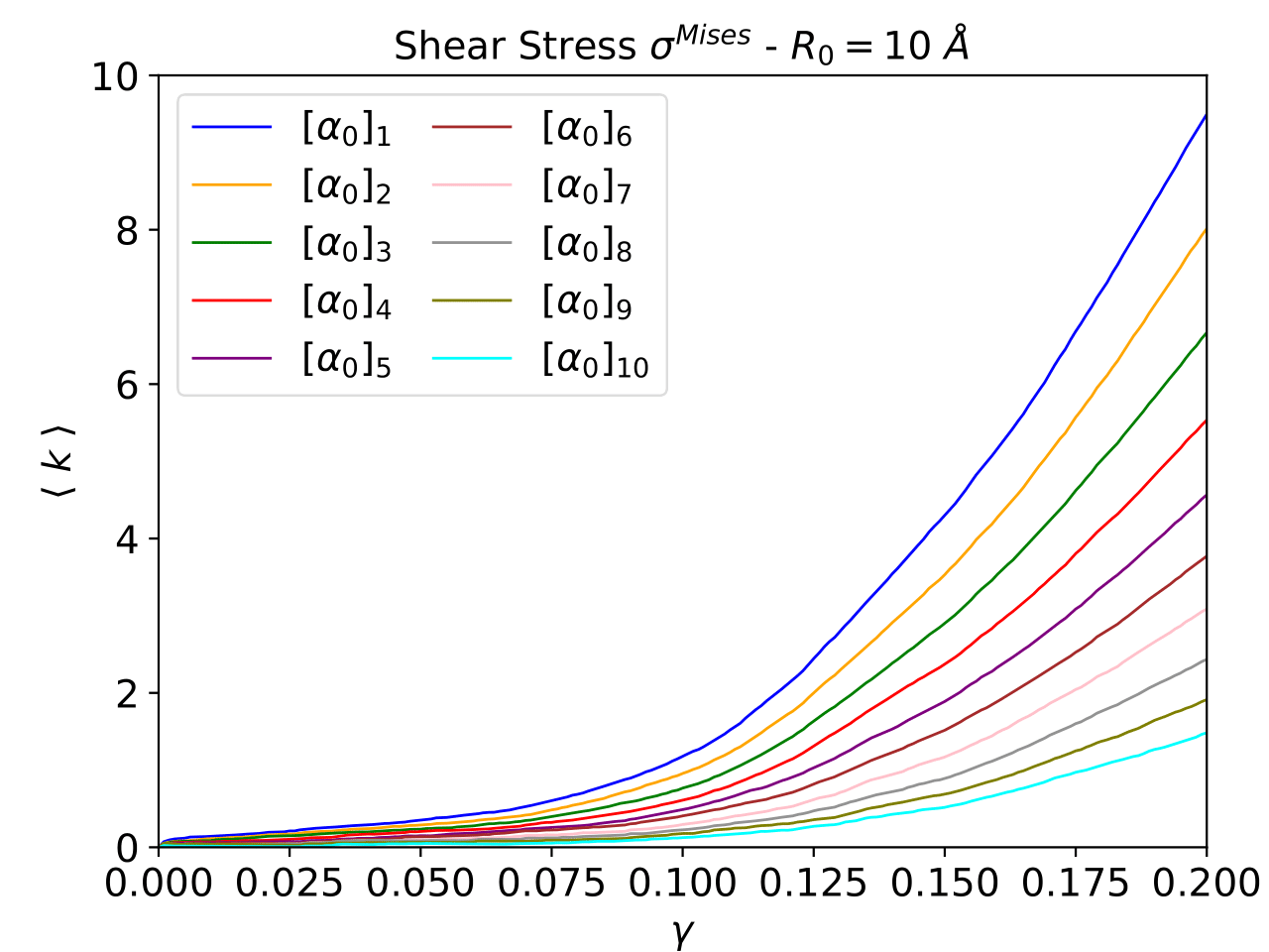
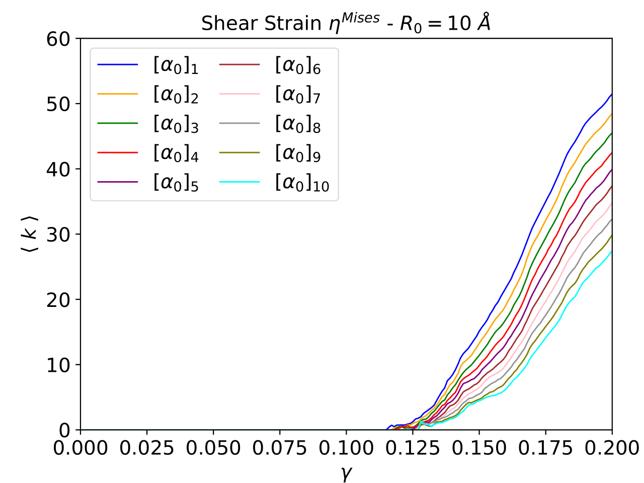
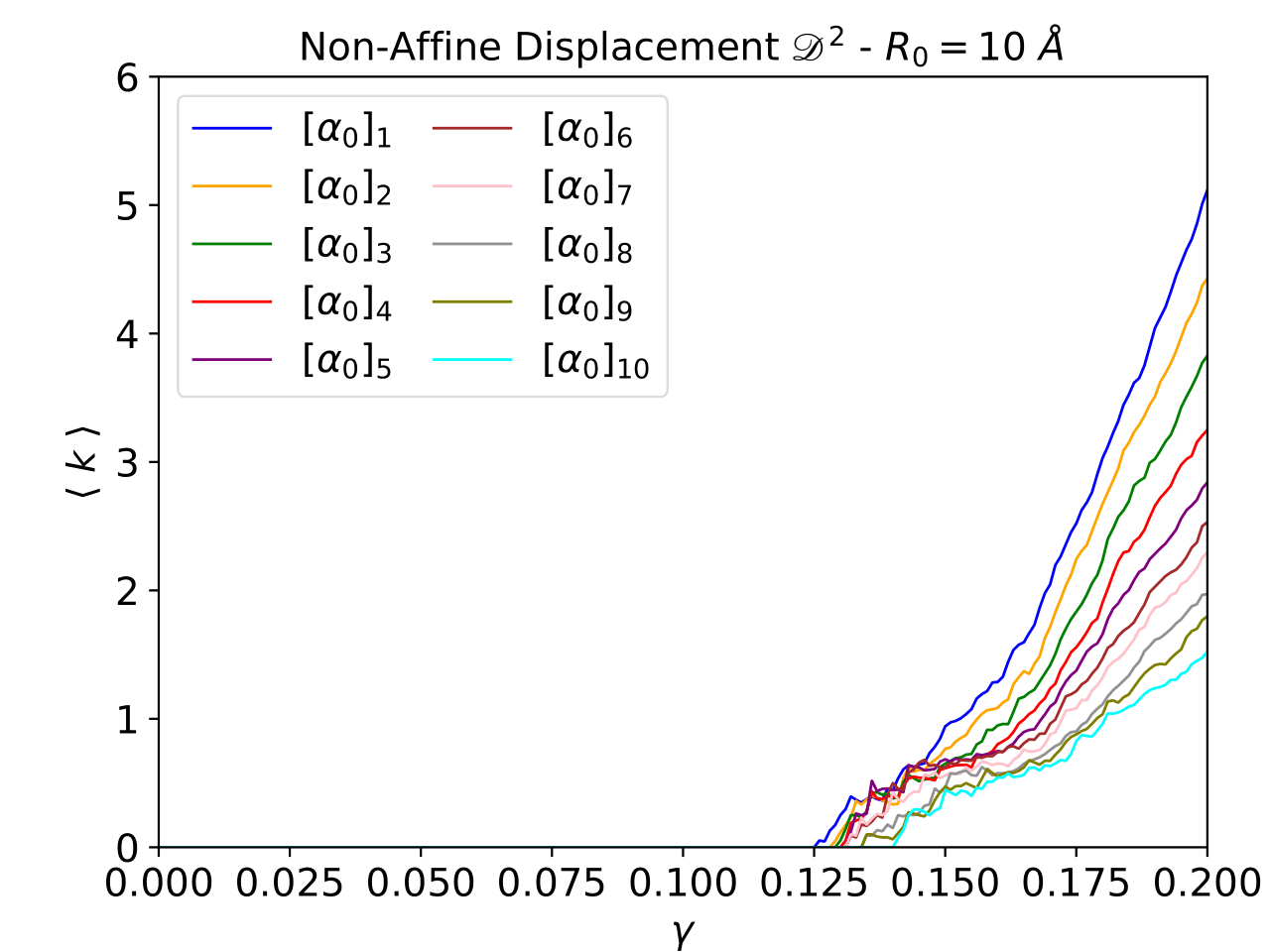
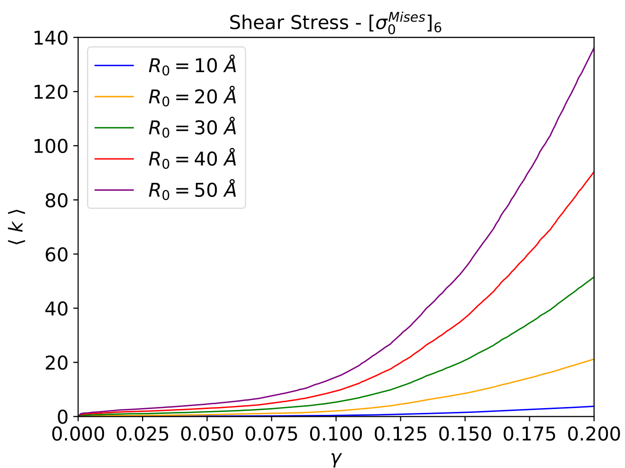
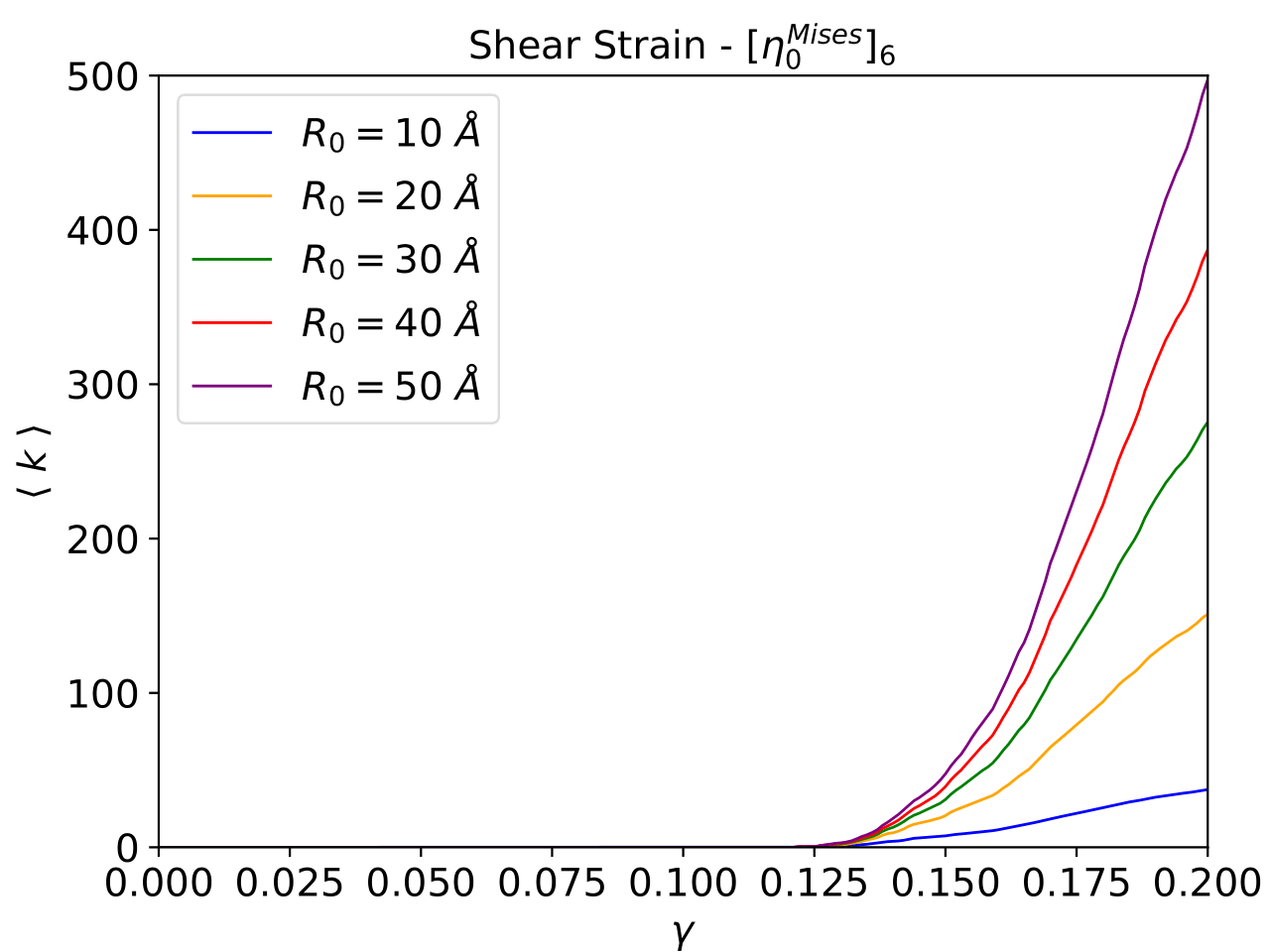
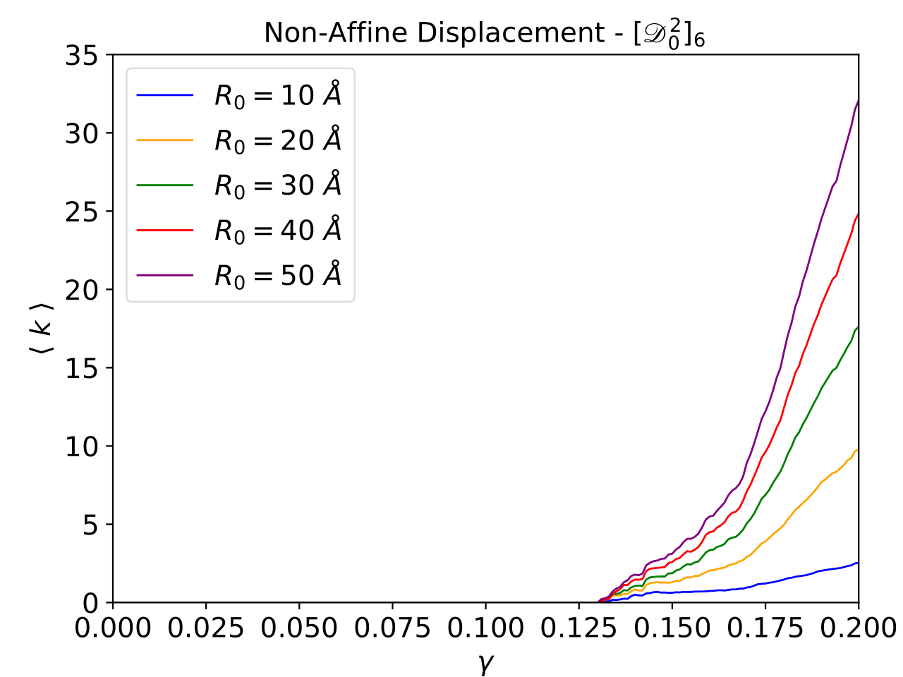
Figure 10: Average degree $\langle k\rangle$ as a function of strain for different physical descriptors, thresholds, and cutoff radii. Metric computed for CNs built based on the descriptors $\alpha=\{\sigma^{\text{Mises}},\eta^{\text{Mises}},\mathscr{D}^{2}\}$. Plots in the first row show a comparison of the $\langle k\rangle$ calculated using different thresholds at a fixed cutoff radius $R_{0}=10$ Å. For all cases, to a higher threshold value, lower is the network average degree, since the population of vertices and edges decrease. Plots in the second row show a comparison of the $\langle k\rangle$ calculated using different cutoff radii with a fixed threshold (depending on the descriptor). For all cases, using a larger cutoff radius increases the degreee since connections increase.

Numerically, the average degree has been the easiest metric to calculate, since we only need to count the number of vertices and edges of the networks constructed for each strain value $\gamma$. As seen in Figure (10), this metric reports different results depending on the descriptor used. For example, for networks with $\alpha=\sigma^{\text{Mises}}$, the degree exhibits a monotonically increasing behavior for all deformation regimen, increasing its slope rate when plastic events give rise to the SB. This microscopic phenomenon of energy dissipation due to irreversible deformations is captured by the degree, a simple and purely topological element, which regardless of the structure of the network, tells us about a macroscopic response suffered by the system. For this type of network, the increase of average degree can be interpreted as an increase in the internal energy of the system due to atomic displacements. For elastic deformations, the atoms oscillate around their equilibrium point (low degree), while for plastic deformations, the atoms become progressively disordered, and some migrate due to the failure caused by the STZs, increasing internal energy (increasing degree).

Similar to networks with $\alpha=\eta^{\text{Mises}}$ and $\alpha=\mathscr{D}^{2}$, the degree increases but only when the system has developed the SBs and the creep zone. This has happened because the thresholds used have not been low enough to capture atoms in another deformation level. In other words, for the elasto-plastic regime, the atoms do not show a Shear Strain or a Non-Affine Displacement comparable to the considered thresholds. Basically, the network built for these descriptors is formed by the atoms that live in the SBs. Therefore, the degree for these cases quantifies the increase of irreversible deformations as shown in the maps of Figure (4).

In Figure (10) we also show an example of how the degree changes depending on the different cutoff radii for a fixed threshold. We see that regardless of the radius, the degree always tends to increase, but with different slope rates, which tells us that for this methodology, physical phenomena in the order between 10-50 Å, do not show a difference beyond values that the degree takes. However, we have observed that for smaller radii and thresholds even larger than $[\sigma^{\text{Mises}}_{0}]_{16}$ (only for $\alpha=\sigma^{\text{ Mises}}$), the degree is no longer monotonically increasing, but fluctuates.

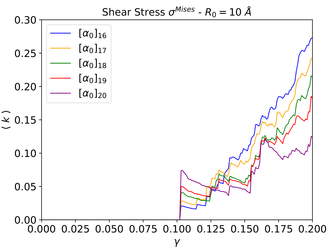
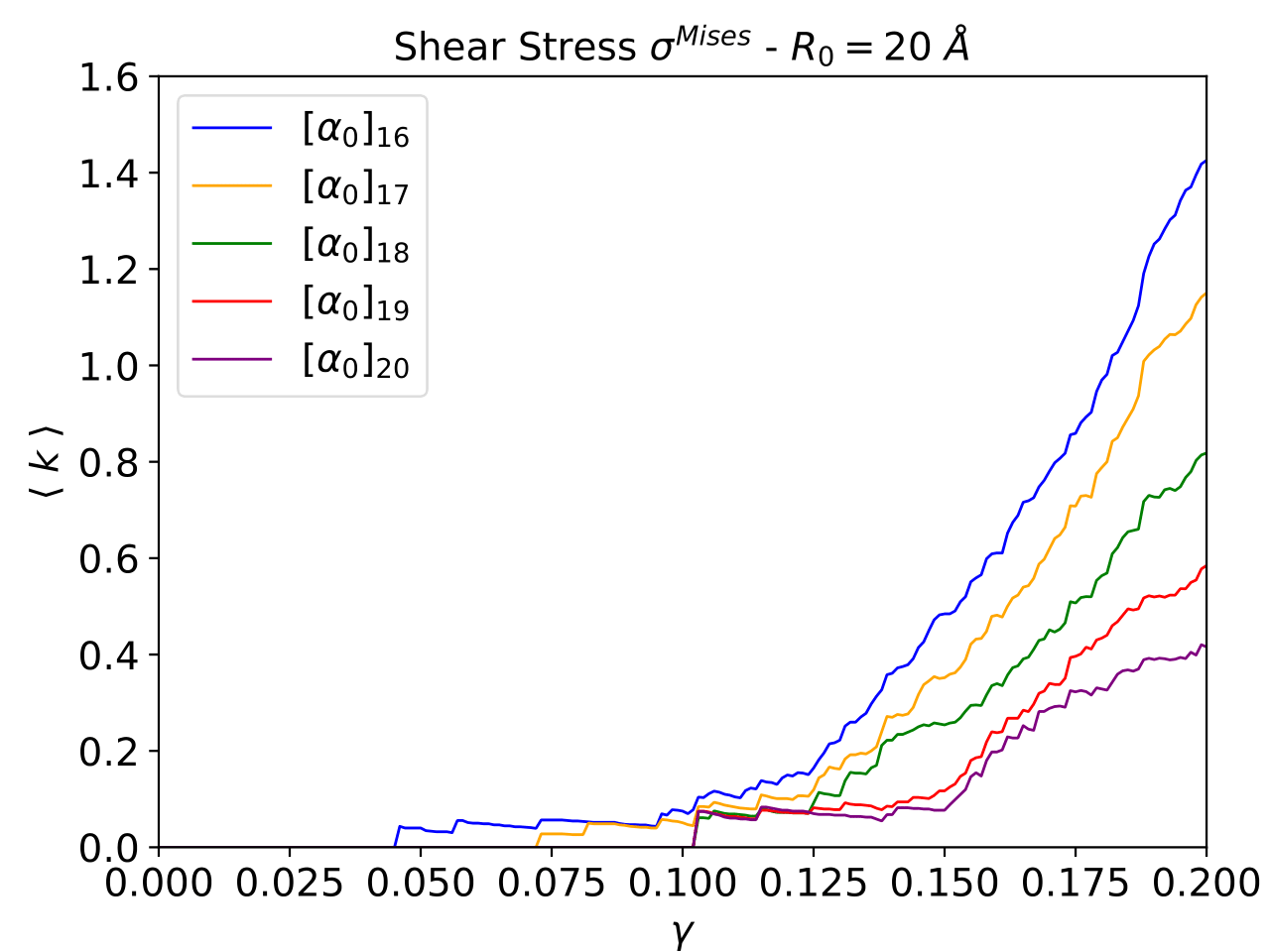
Figure 11: Average degree $\langle k\rangle$ as a function of strain for a network with $\alpha=\sigma^{\text{Mises}}$ for different thresholds and cutoff radii $R_{0}=10\text{ \AA}$ and $R_{0}=20\text{ \AA}$.

The average degree for a network with $\sigma^{\text{Mises}}$ in Figure (10), increases as strain increases regardless of the threshold used. These curves are smooth with a certain slope rate that could be calculated with a numerical derivative. However, if we build these networks with even higher thresholds, we obtain an interesting result to analyze. In Figure (11) the average degree calculated with a $R_{0}=10\text{ \AA}$ shows less smoothness than the previous results and a variable slope rate, but this it is only a consequence of the physics that the metric is representing. With these parameters, the network begins to grow once the SB has been located ($\gamma\sim 0.1$), revealing that there are highly stressed atoms involved in the construction of the graph. According to our previous interpretation, the average degree is like an internal energy of the system, being in this case, the energy that these highly stressed atoms contribute, but the interesting result is when that energy is released via decrease of the degree. For the different thresholds that have been used in Figure (11), they all exhibit degree drops, which we physically interpret as a release of internal energy, causing an increase of temperature. This result proves the existence of nanofractures/avalanches precisely due to those highly stressed atoms.

The results obtained for the case $R_{0}=20\text{ \AA}$ still show some degree drops, but they are less and less noticeable. This is already a sign that the network begins to hide some details that occur locally and only show the progressive increase in degree tending to smoothness and a constant slope rate. The average degree for networks with $\alpha=\eta^{\text{Mises}}$ and $\alpha=\mathscr{D}^{2}$ constructed for higher thresholds has also been revised, but does not reveal interesting results. given the lack of vertices. Physically, there are not enough highly deformed atoms to build a network.

The next metric that we study are the clustering coefficient of the network as a function of strain. The parameters we have selected for this case are: For the Shear Stress, $[\sigma_{0}^{\text{Mises}}]_{11}$ , for the Shear Strain, $[\eta_{0}^{\text{Mises}}]_{15}$ and for the Non-Affine Displacement, $[\mathscr{D}^{2}]_{6}$.

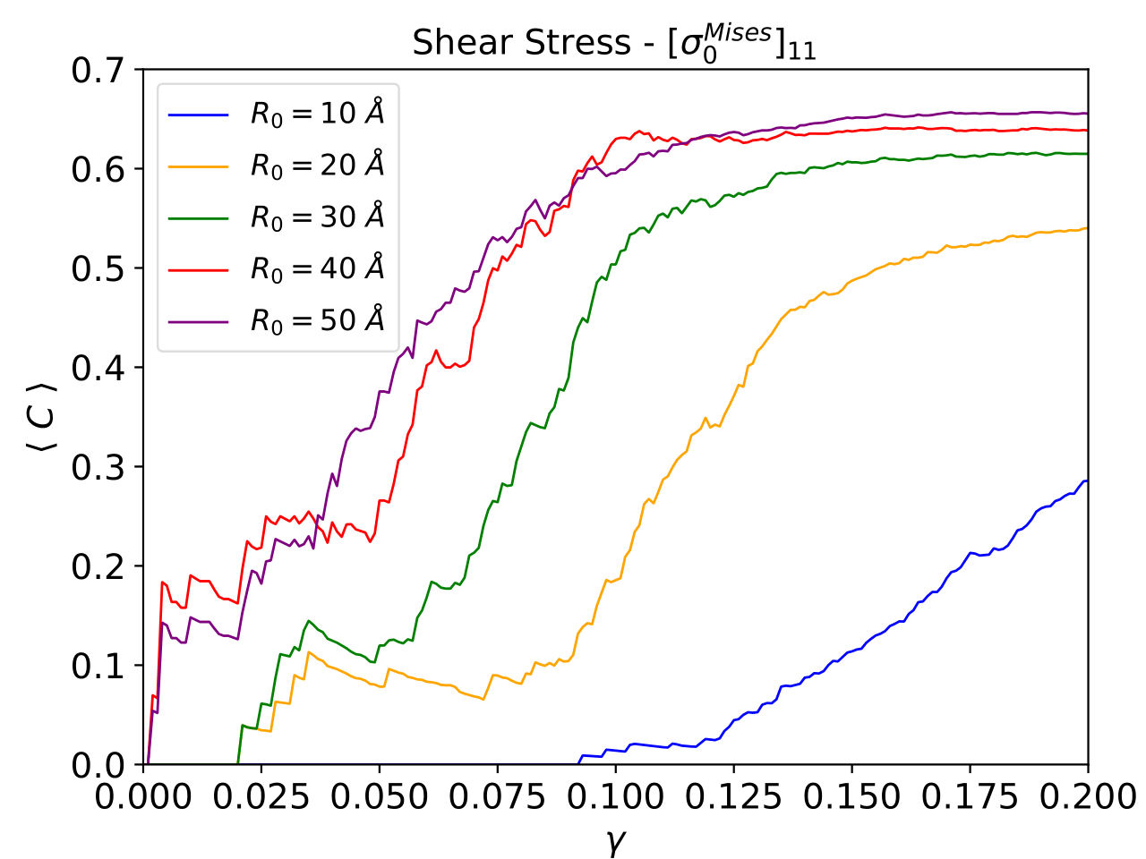
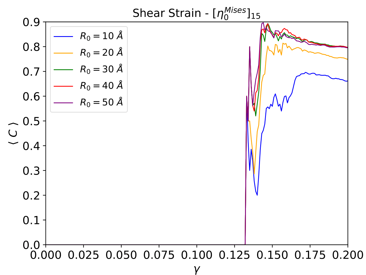
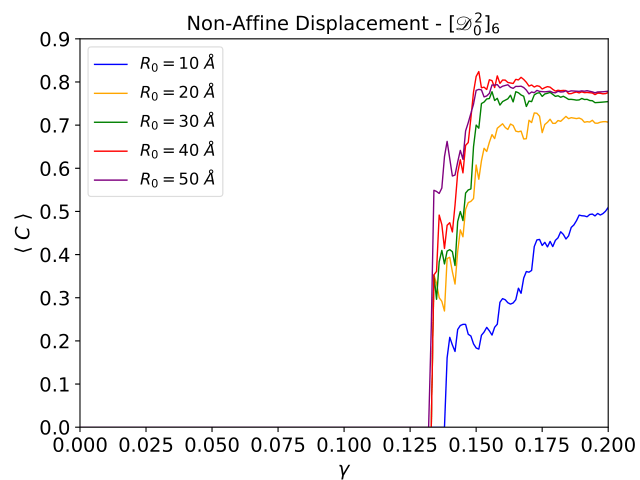
Figure 12: Average clustering coefficient $\langle C\rangle$ as a function of strain for different cutoff radii and physical descriptors. Metric calculated for CNs built based on the descriptors $\alpha=\{\sigma^{\text{Mises}},\eta^{\text{Mises}},\mathscr{D}^{2}\}$. Comparison of the average clustering coefficients calculated for different cutoff radii with a fixed threshold (depending on the descriptor).

In this case, we compute the clustering coefficient of the network as the sum of the clustering coefficient of each vertex averaged by the number of vertices for each strain value $\gamma$. This coefficient is a measure of information about the local structure of the network and how the vertices are connected to each other. In particular, it measures the probability that the neighbors of a vertex are also neighbors of each other, so the range of values it takes is between $0$ and $1$. Therefore, the average over the network of this measure provides information about the global structure, and a characterization of how robust is the network against threats such as vertex and/or edge extraction.

In Figure (12) we present the results for the average clustering coefficient as a function of strain for the three descriptors. For networks with $\alpha=\sigma^{\text{Mises}}$, clustering of vertices takes place from the start, indicating an increase as strain increases. Although the curves are not smooth, it is possible to identify some important variations depending on the different deformation regimes. For the cutoff radius $R_{0}=20\text{ \AA}$ we see this metric suffers a considerable increase during the SB location, while for $R_{0}>20\text{ \AA}$, the clustering saturates to $\langle C\rangle\sim 0.6$. This occurs because the clustering coefficient intensifies after the elastic limit in response to the formation of the STZs and SBs.

For the other descriptors, the average clustering undergoes a drastic increase since the first vertices and edges appear in the graph. We remember that the atoms that map to these vertices are those that live in the SB, therefore the interactions in time are more robust, which increases the clustering up to a value of $\langle C\rangle\sim 0.9-0.7$. By means of this metric, these networks perfectly represent the SB showing how strong is the interaction between its atoms. The above invites us to think about how robust are these networks and how they will respond to attacks on the vertices or edges. For example, what happens to the clustering coefficient if we remove any vertex or edge? What happens to the connectivity if we attack the network in this way? Physically, removing vertices/atoms from the network/cell will prevent the location of SB and/or fracture of the material?. These are some questions that would be interesting to address.

The last metrics we study are the betweenness centrality and the closeness centrality of the network as a function of strain. The parameters that we have selected for this case are: For the Shear Stress, $[\sigma_{0}^{\text{Mises}}]_{8}$, for the Shear Strain, $[\eta_{0}^{\text{Mises}}]_{20}$ and for the Non-Affine Displacement, $[\mathscr{D}^{2}]_{6}$.

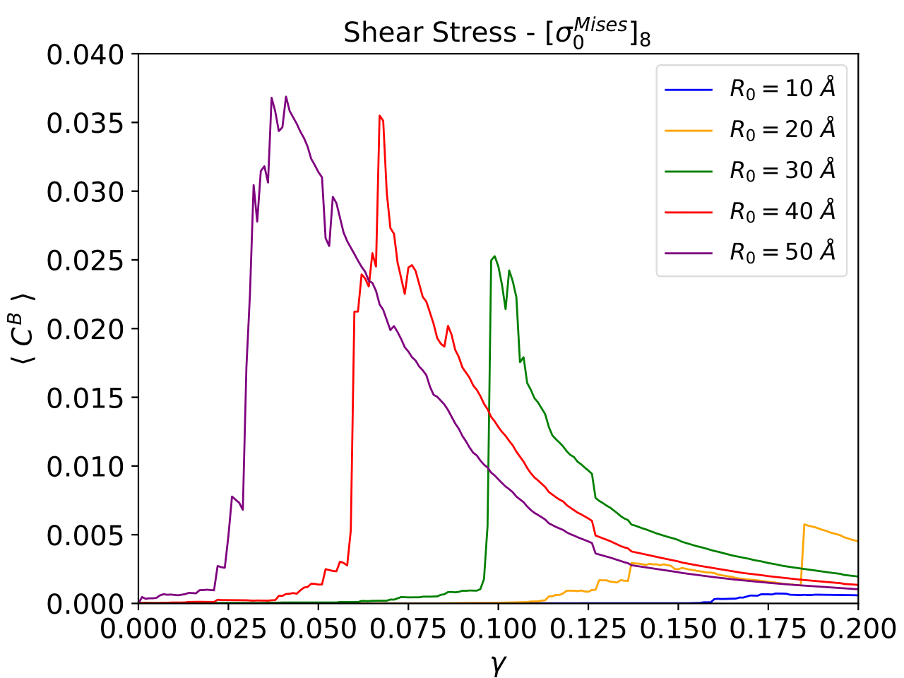
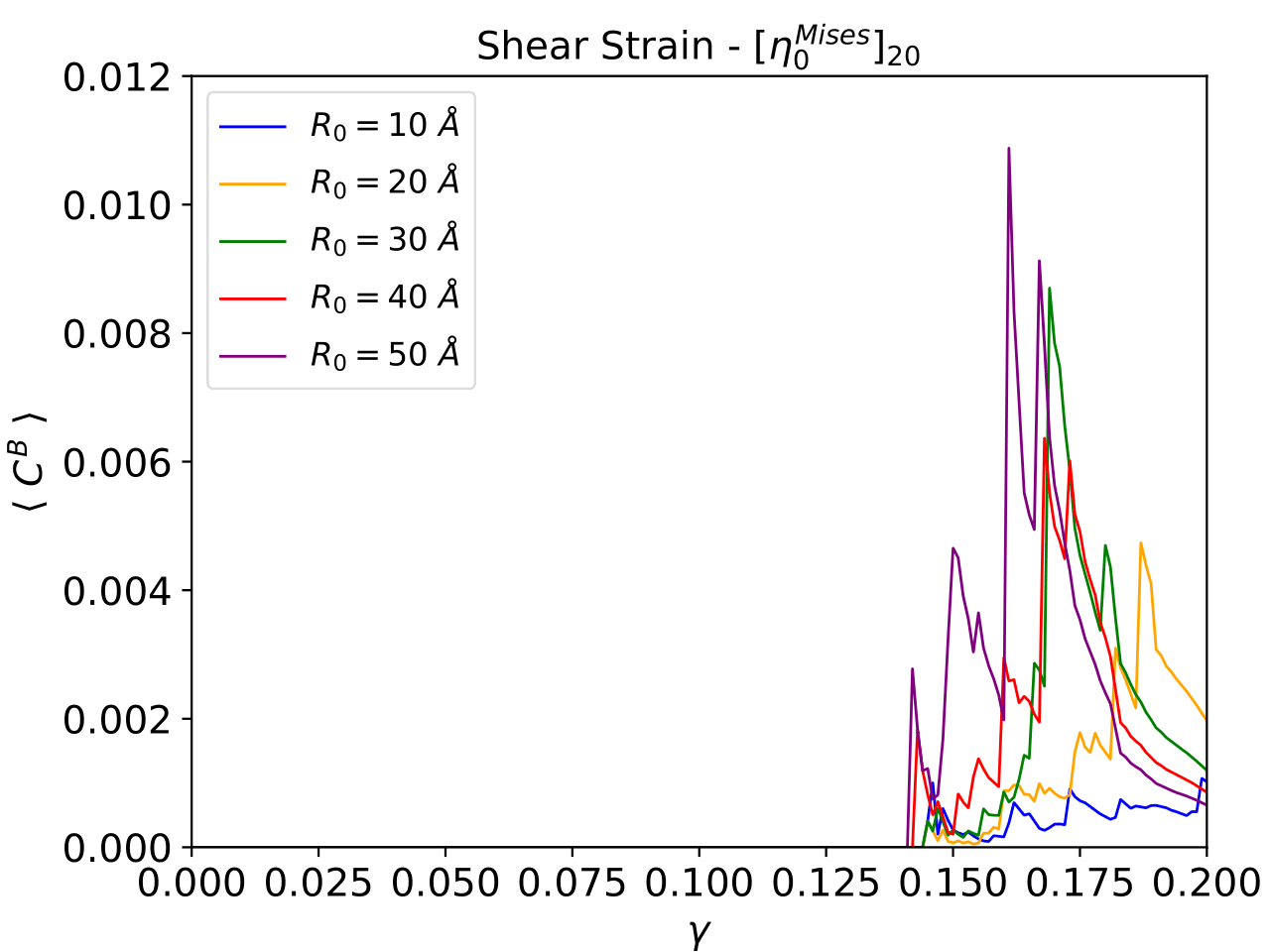
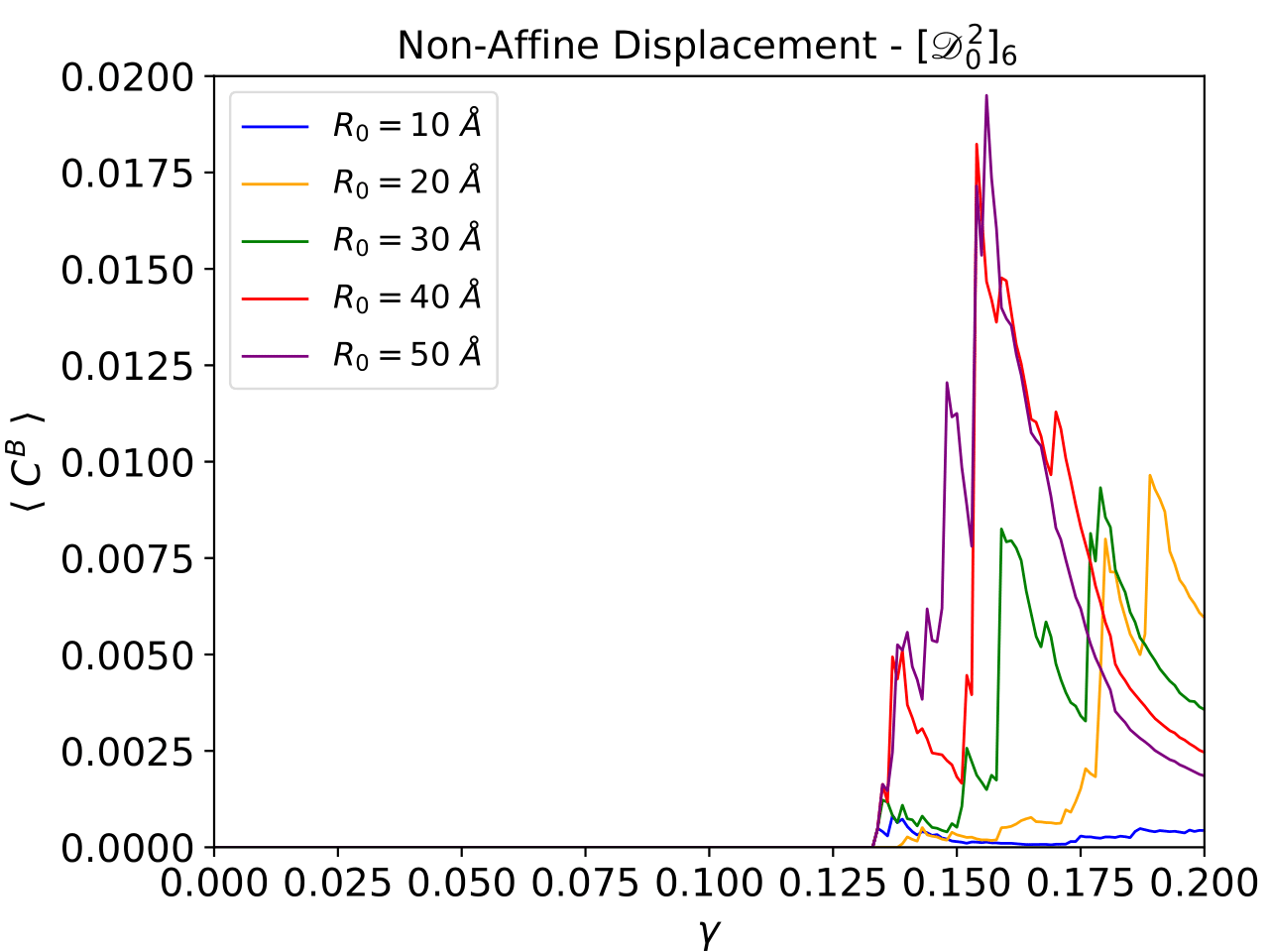
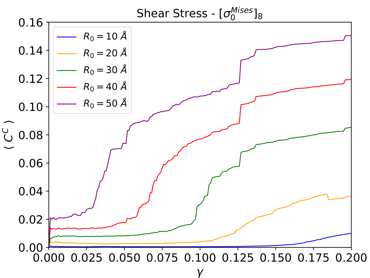
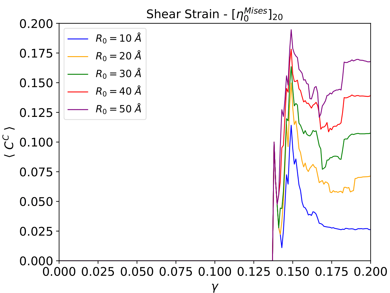
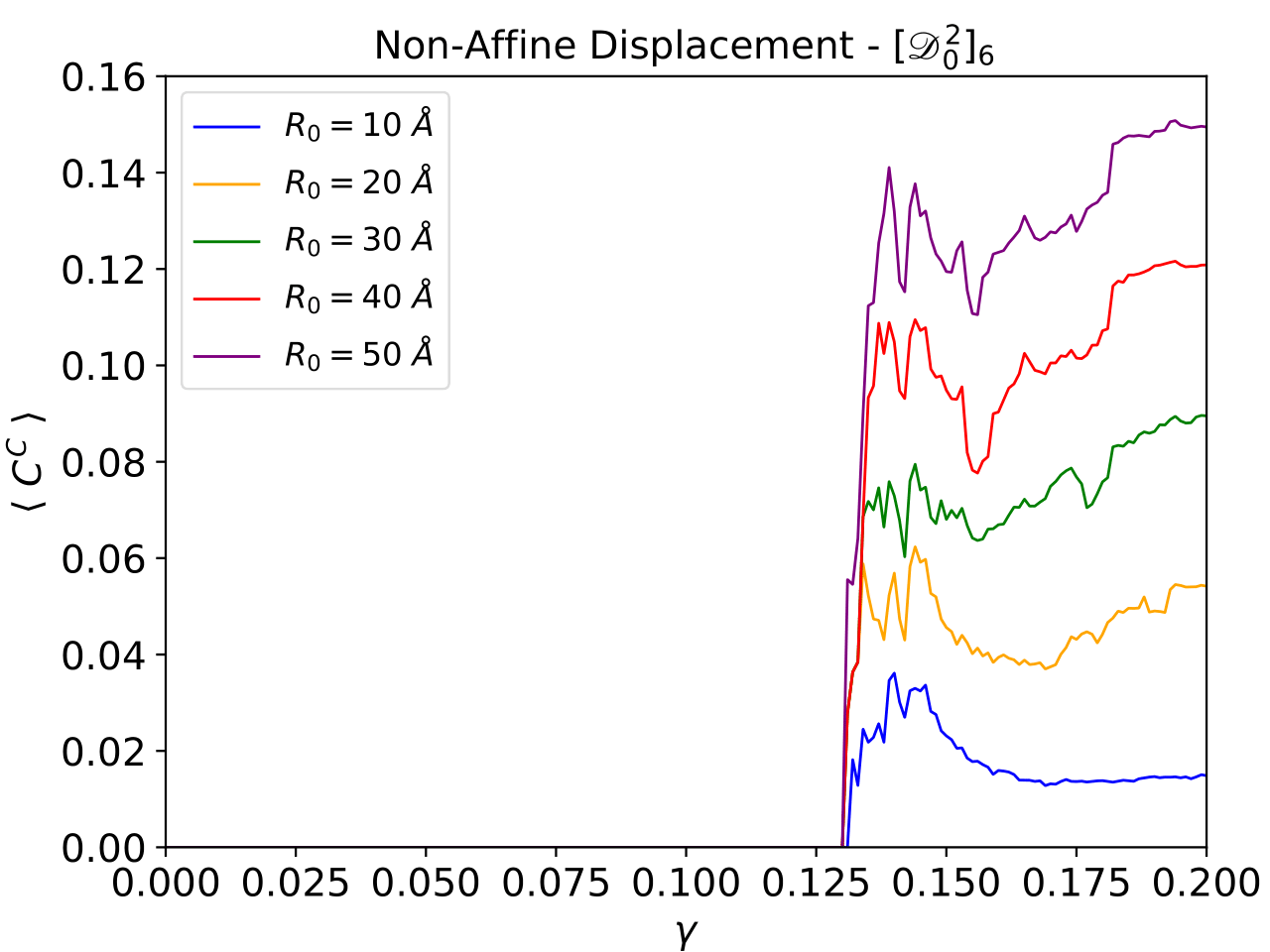
Figure 13: Average betweenness $\langle C^{B}\rangle$ and closeness $\langle C^{C}\rangle$ centrality as a function of strain for different cutoff radii and physical descriptors. Metric calculated for CNs built based on the descriptors $\alpha=\{\sigma^{\text{Mises}},\eta^{\text{Mises}},\mathscr{D}^{2}\}$. Plots in the first row show a comparison of the average betweeness centrality calculated for different cutoff radii at a fixed threshold (depending on the descriptor). Plots in the second row show the same as above but now for the average closeness centrality.

We have calculated the average betweenness and closeness centrality of the network as the independent sum of the betweenness and closeness of each vertex averaged by the number of vertices for each strain value $\gamma$. We know that these metrics quantify the importance of the vertices, providing a local characterization of the network. Despite this, the average, which indicates a global property, allows us to obtaine information about the vulnerability and robustness of the network, which is what interests us most in this context. In Figure (13) we have a very interesting result for networks with $\alpha=\sigma^{\text{Mises}}$ and cutoff radii $R_{=}\{30,40,50\}$ Å. We see that the average betweennes reaches a maximum and then decreases, while the closeness only increases for the entire strain interval. A valid interpretation for this decrease in the betweenness of the network is that from a moment on, important vertices that fulfill the role of bridges stop appearing, the network becomes denser, but not necessarily with edges that are what give it the quality of importance to the vertices. Even so, this does not imply that the network is more vulnerable. Direct evidence of this is the result that we obtain for the closeness of the network. The increase in this metric is proof that shorter paths appear that give importance to the vertices, making the network more robust. With this result we are in the presence of the fact that there are and exist vertices/atoms that mediate the interaction of other groups of atoms/subnetworks or communities, which is physically the topological representation of the interaction between different STZs and that finally collapse in a SB.

In the case of networks with $\alpha=\eta^{\text{Mises}}$ and $\alpha=\mathscr{D}^{2}$, it is not possible to capture a clear result. Given that the networks begin their growth once the material has fractured, we cannot draw any conclusions about what precedes this phenomenon, therefore the fluctuations of these metrics are only a response to an uncontrolled growth of vertices and edges as a result of the high strains achieved.

5.1 Complex networks and spatial distribution of topological metrics

Until now we have only presented the compute of topological metrics as a function of strain, analyzing each curve with respect to the physical phenomena involved, but to have a more complete study, we present a visual representation of these CNs once the simulation is finished. For this, we have used the Python NetworkX module [47] to graph these networks.

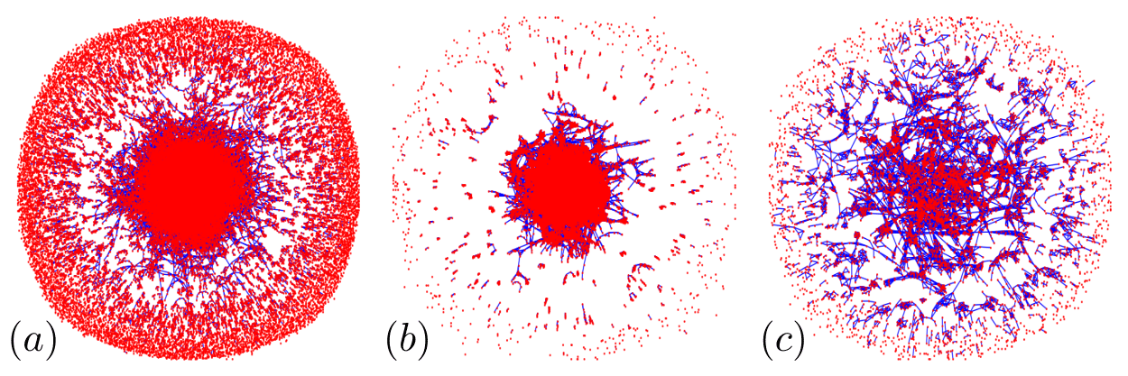
Figure 14: Undirected CNs resulting at the end of the deformation process. The networks were built with the parameter set (a) $\{\sigma^{\text{Mises}},[\sigma^{\text{Mises}}_{0}]_{6},10\text{ \AA}\}$, (b) $\{\eta^{\text{Mises}},[\eta^{\text{Mises}}_{0}]_{6},10\text{ \AA}\}$ and (c) $\{\mathscr{D}^{2},[\mathscr{D}^{2}_{0}]_{6},10\text{ \AA}\}$. The red points are the vertices and the blue lines are the edges.

In Figure (14) we show an example of how looks like each network built for the three $\alpha$ descriptors once the deformation process is completed. Each network acquires a large population of vertices and edges, where we see that the representation algorithm places vertices in the center and the perimeter, depending on the degree of interaction it has with its neighbors. The center of each network is where the highest density of dominant edges and vertices is located. A cluster of vertices and edges is the only thing that highlights for networks with $\alpha=\{\sigma^{\text{Mises}},\eta^{\text{Mises}}\}$. Due to the high number of interactions, it is visually difficult to identify if there are preferential connections or some degree of randomness in the edge distribution, but the most interesting case is the network with $\alpha=\mathscr{D}^{2}$, since thanks to its lower vertex density (compared to the other two cases), we can identify that there are sub-networks or small communities that have their own local interaction, and even community interaction.

The interesting about this is that through a mathematical methodology based on graph theory, it is possible to characterize microscopic and macroscopic properties of a system subject to deformation. Basically, we are describing the physical phenomena involved in the elasto-plastic regime using the abstraction of topological metrics and a representation technique via CNs. We well know that these networks are topological structures and that their properties do not depend on their representation, therefore, we present the same previous graphs but now with the vertices located in relation to their respective atom in the simulation cell. In these cases, we have eliminated the edges since the vertices are colored according to the corresponding topological metrics that we have studied.

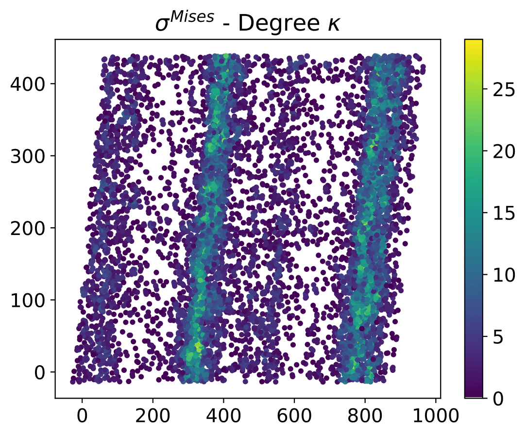
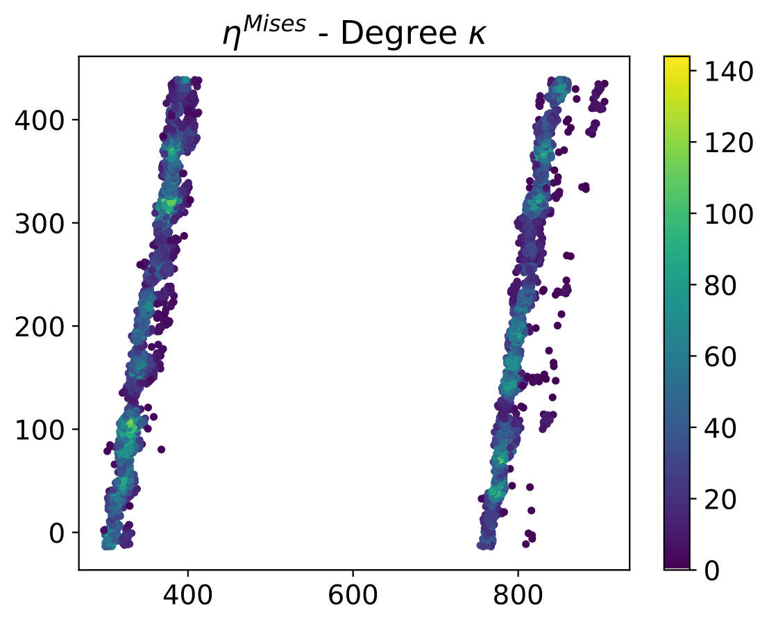
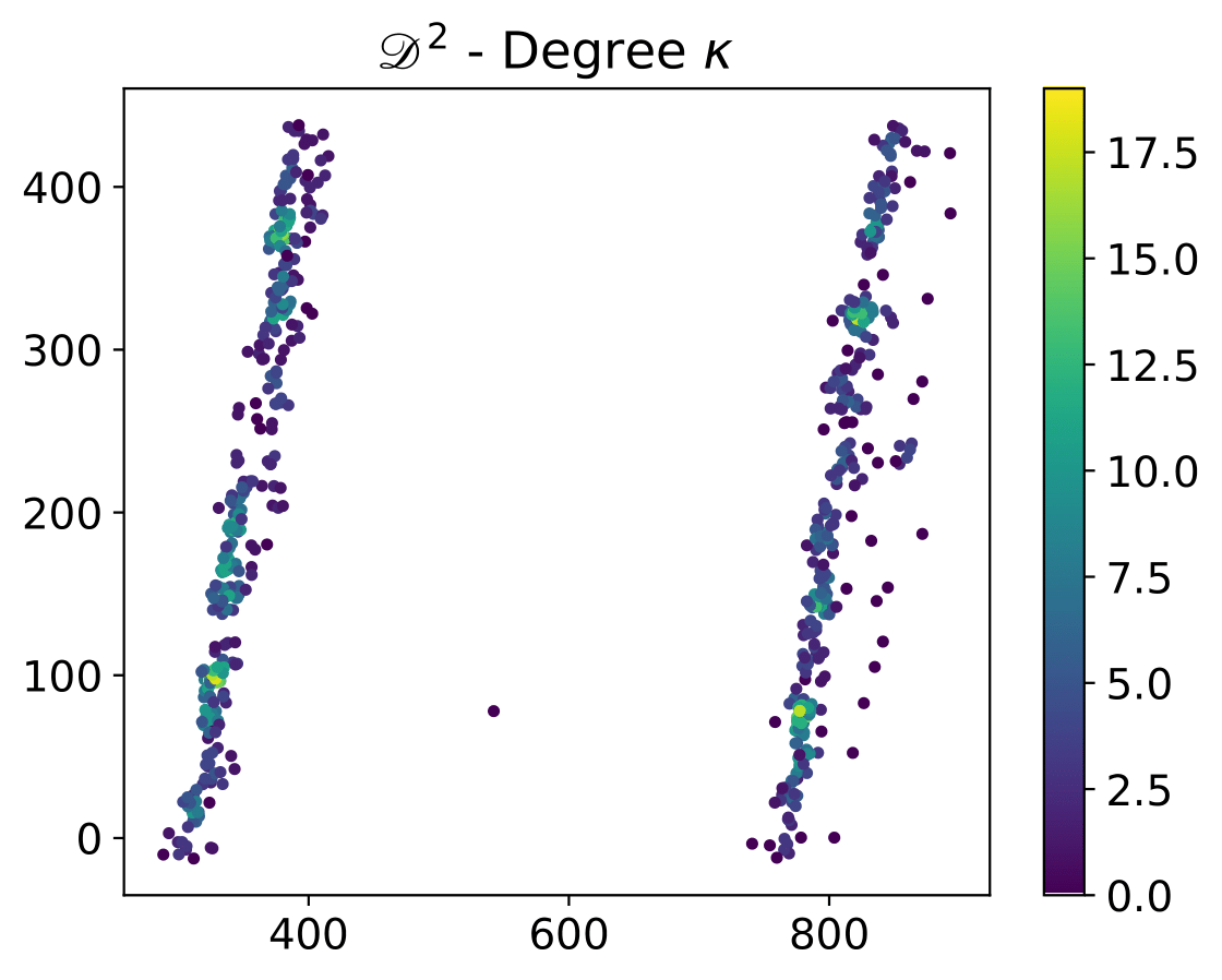
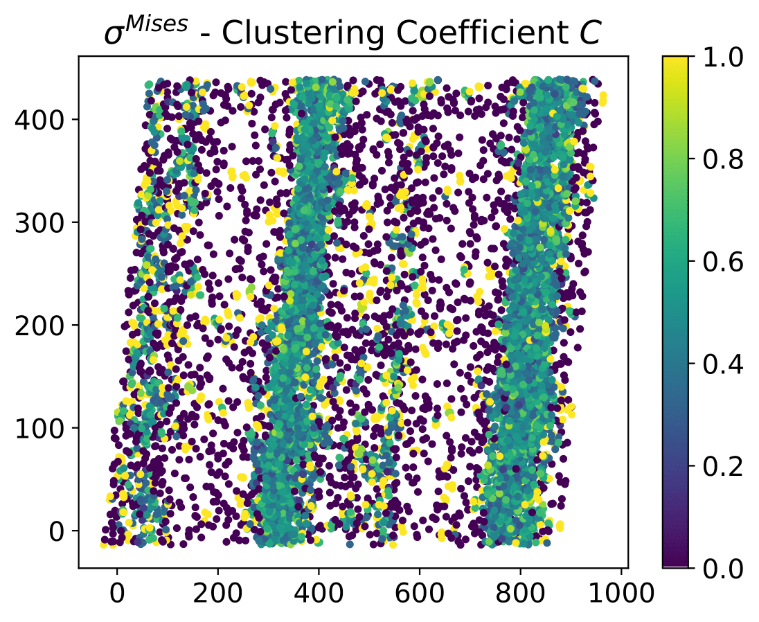
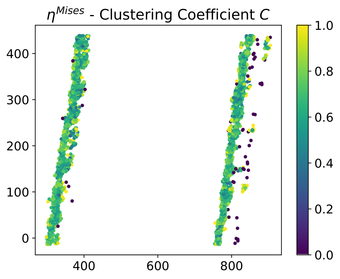
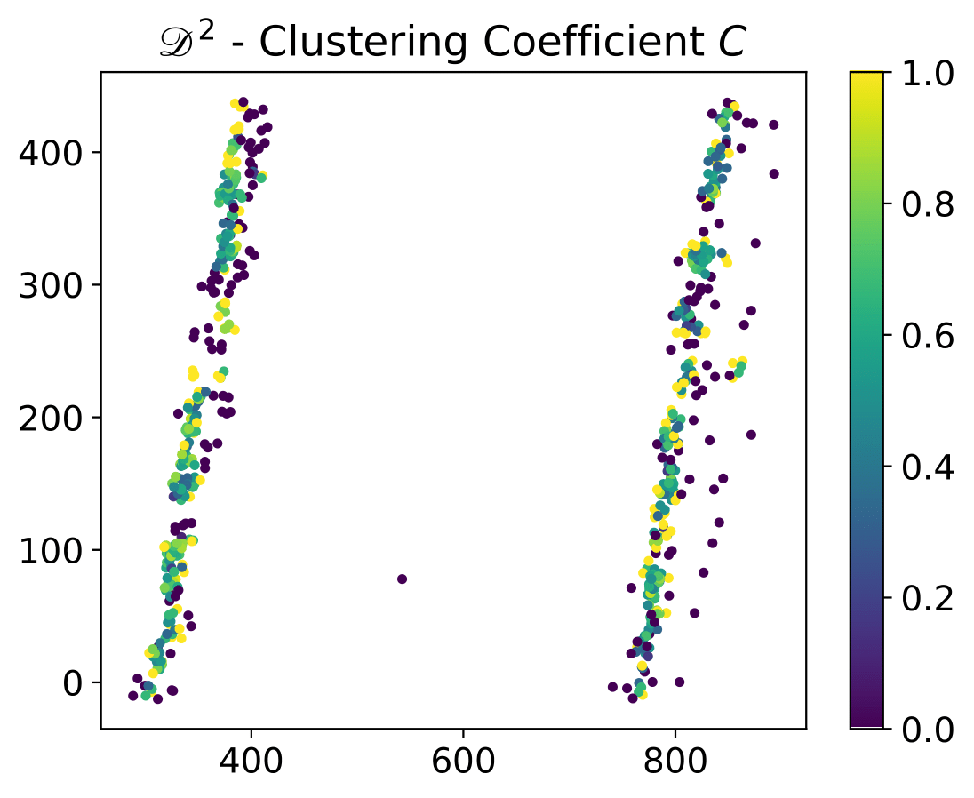
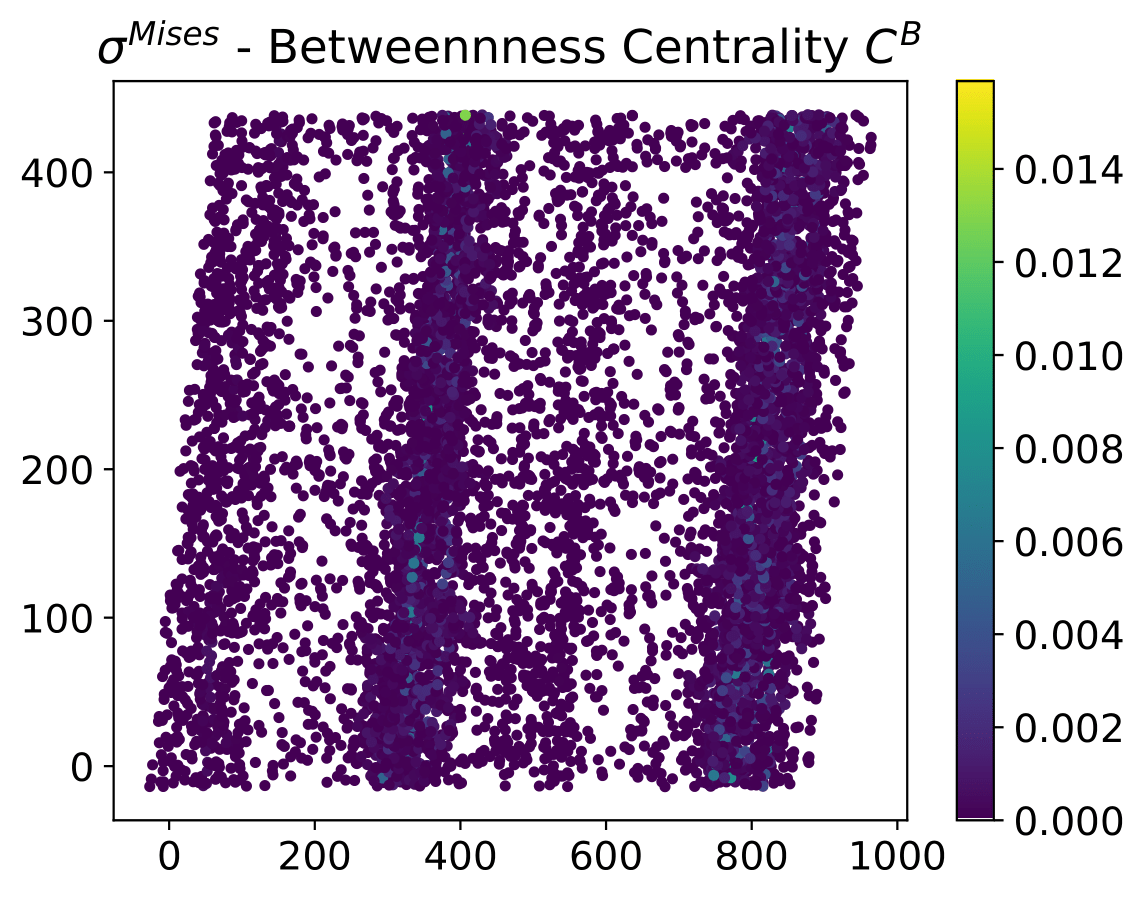
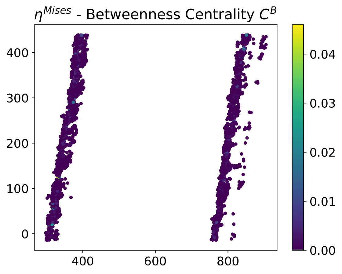
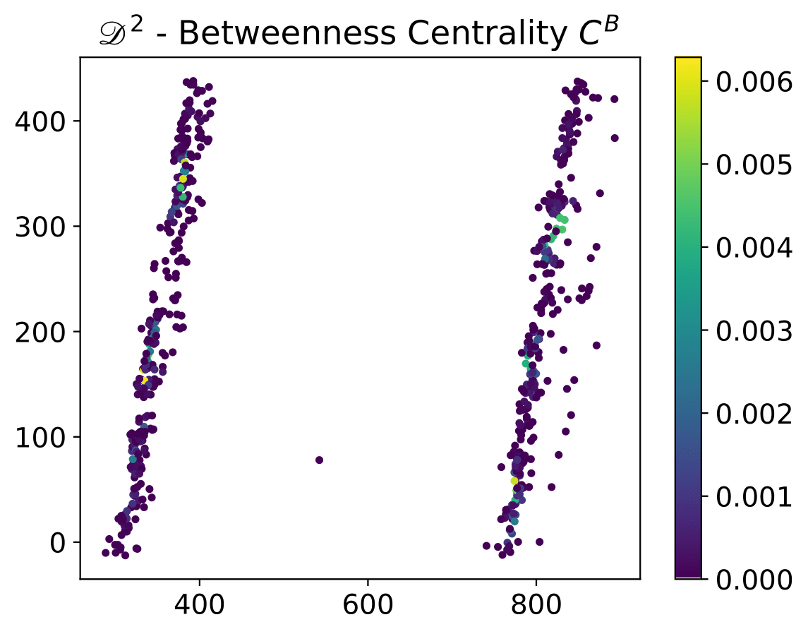
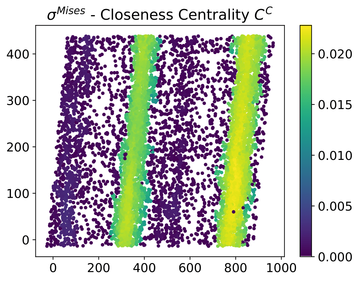
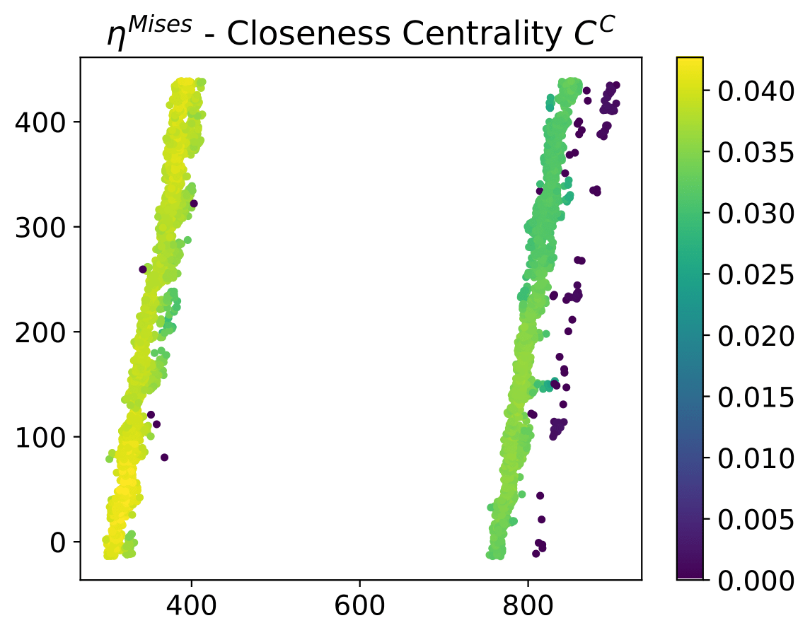
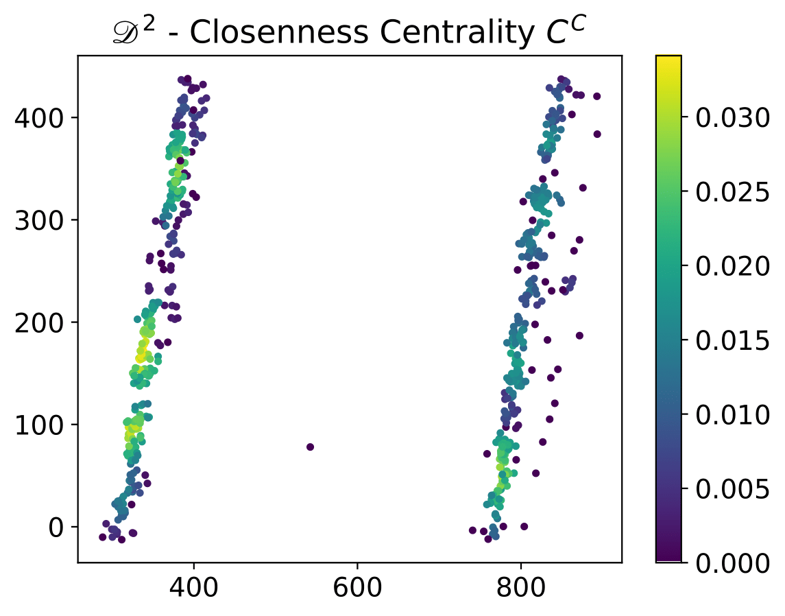
Figure 15: Spatial distribution (CN without edges) of the metrics calculated for the networks of Figure (14) under the topological representation where the vertices are located in the position of their corresponding atom for the instant that the system reaches the deformation state $\gamma=0.20$. A color bar is included to record the range of values that each metric takes.

The results that we have obtained for the spatial distribution of the metrics show that our methodology, based on graph theory and CNs, has allowed a microscopic characterization of the deformation and identification of plastic events that give rise to the SB and eventual material fracture. Figure (15) shows the networks for the three descriptors and for each one, the atoms are colored according to the degree, the clustering coefficient, the betweenness centrality and the closeness centrality, where each metric shows that there is a area of the material where the interactions are more intense and complex, either due to the levels of energy released by the plastic deformation (degree), or due to the regrouping and packing by irreversible movements of the atoms (clustering), or due to the interaction collective group of atoms (centrality) known as STZs.

The relevant result here is that such metrics have been able to signal the location of the SB generated by the deformation process, suggesting this description via CNs to study the phenomenon of plasticity in amorphous materials.

6 Conclusions

In present work we have performed a shear deformation of the Cu₅₀Zr₅₀ metallic glass using molecular dynamic simulations and by means statistical analysis and application of a complex network model, we have studied the plasticity in this type of amorphous material. Our results suggest the complex network description may be a useful tool for the study of material properties and description of physical phenomena that occur at the microscopic level.

The statistical analysis of the physical descriptors has allowed a better understanding of the physics of the system under a deformation process. The probability density functions of these descriptors were calculated to gain insight into the randomness of the parameters. However, the most notable result is the time series of the gini coefficient. This measure together with the Lorenz curves show considerable changes precisely in regimes where a physical phenomenon occurs. For example, in the elasto-plastic transition $\gamma\sim 0.045$, in the plastic regime $0.045<\gamma$, in the location of the SB $\gamma\sim 0.095$ and eventual fracture of the material $\gamma\sim 0.130$. Basically, the microscopic statistical analysis of the descriptors has predicted what happens at the macroscopic level as a consequence of the deformation.

The methodology based on complex networks, where the atomic configurations of the system are mapped to a graph that increases in number of vertices and edges, added to the calculation of topological metrics, has turned out to be a very useful mathematical tool for the microscopic characterization of deformation. In this research, we develop the calculation of the degree, the clustering coefficient and measures of centrality such as betweennes and closeness for the characterization of the plastic events that transit during the deformation. The topological structure of the networks and the metrics have shown interesting results as proof of the existence of energy dissipation due to irreversible movements in the plastic regime and, as a consequence, the increase in temperature (increase in degree), as well as the evidence of communities or groups of atoms that interact among themselves and other groups, providing a new justification for the hypothesis of shear transformation zones as a fundamental element in the theory of plasticity in amorphous materials.

Because of amorphous systems exhibit greater complexity at the atomic configuration level, efforts to understand their properties using condensed matter physics theories is still a challenge. Therefore, the complex network techniques presented here represents an alternative, strong technique, to study the physical properties of these systems.

CRediT authorship contribution statement

F. Corvacho: Conceptualization, Methodology, Software, Formal analysis, Data Curation, Writing (Original Draft), Visualization. V. Muñoz: Conceptualization, Methodology, Formal analysis, Writing (Review & Editing), Supervision, Project administration. M. Sepúlveda-Macías: Software, Resources, Writing (Review & Editing). G. Gutiérrez: Writing (Review & Editing), Supervision.

Declaration of Competing Interest

The authors declare that they have no known competing financial interests or personal relationships that could have appeared to influence the work reported in this paper.

Declaration of Generative AI and AI-assisted technologies in the writing process

The autors declare that they have not used any type of AI technologies in this paper.

Additional Information

Correspondence and requests for materials should be addressed to Fernando Corvacho.

References

- [1] W.H. Wang. Bulk metallic glasses with functional physical properties. Advanced Materials, 21(45):4524–4544, 2009.
- [2] P. Tiberto, M. Baricco, E. Olivetti, and R. Piccin. Magnetic properties of bulk metallic glasses. Advanced Engineering Materials, 9(6):468–474, 2007.
- [3] A.L. Greer. Metallic glasses. Science, 267(5206):1947–1953, 1995.
- [4] T.R. Anantharaman. Metallic glasses: production, properties and applications. Trans Tech Publ, 1984.
- [5] M.F. Ashby and A.L. Greer. Metallic glasses as structural materials. Scripta Materialia, 54(3):321–326, 2006.
- [6] W. Klement, R.H. Willens, and P. Duwez. Non-crystalline structure in solidified gold–silicon alloys. Nature, 187(4740):869–870, 1960.
- [7] A. Peker and W.L. Johnson. A highly processable metallic glass: . Applied Physics Letters, 63(17):2342–2344, 1993.
- [8] A. Inoue, Y. Horio, and T. Masumoto. New amorphous Al–Ni–Fe and Al–Ni–Co alloys. Materials Transactions, JIM, 34(1):85–88, 1993.
- [9] C. Suryanarayana and A. Inoue. Bulk metallic glasses. CRC Press, 2017.
- [10] M.M. Trexler and N.N. Thadhani. Mechanical properties of bulk metallic glasses. Progress in Materials Science, 55(8):759–839, 2010.
- [11] M. Chen. Mechanical behavior of metallic glasses: Microscopic understanding of strength and ductility. Annu. Rev. Mater. Res., 38:445–469, 2008.
- [12] C.A. Schuh, T.C. Hufnagel, and U. Ramamurty. Mechanical behavior of amorphous alloys. Acta Materialia, 55(12):4067–4109, 2007.
- [13] J. Plummer. Is metallic glass poised to come of age? Nature Materials, 14(6):553–555, 2015.
- [14] A.S. Argon. Plastic deformation in metallic glasses. Acta Metall., 27(1):47–58, 1979.
- [15] M.L. Falk and J.S. Langer. Dynamics of viscoplastic deformation in amorphous solids. Physical Review E, 57(6):7192, 1998.
- [16] F. Shimizu, S. Ogata, and J. Li. Theory of shear banding in metallic glasses and molecular dynamics calculations. Materials Transactions, 2007.
- [17] A.L. Greer, Y.Q. Cheng, and E. Ma. Shear bands in metallic glasses. Materials Science and Engineering: R: Reports, 74(4):71–132, 2013.
- [18] R. Rezaei, C. Deng, M. Shariati, and H. Tavakoli-Anbaran. The ductility and toughness improvement in metallic glass through the dual effects of graphene interface. Journal of Materials Research, 32(2):392, 2017.
- [19] M. Sepulveda-Macias, N. Amigo, and G. Gutierrez. Tensile behavior of metallic glass nanowire with a B2 crystalline precipitate. Physica B: Condensed Matter, 531:64–69, 2018.
- [20] R. Albert and A.-L. Barabási. Statistical mechanics of complex networks. Rev. Mod. Phys., 74(1):47, 2002.
- [21] M.E. Newman, A.-L. Barabási, and D.J. Watts. The structure and dynamics of networks. Princeton University Press, 2006.
- [22] A. Gheibi, H. Safari, and M. Javaherian. The solar flare complex network. The Astrophysical Journal, 847(2):115, 2017.
- [23] M. Gosak, R. Markovič, J. Dolenšek, M.S. Rupnik, M. Marhl, A. Stožer, and M. Perc. Network science of biological systems at different scales: A review. Physics of Life Reviews, 24:118–135, 2018.
- [24] S. Wasserman, K. Faust, et al. Social network analysis: Methods and applications, volume 8. Cambridge University Press, 1994.
- [25] M. Baiesi and M. Paczuski. Complex networks of earthquakes and aftershocks. Nonlinear Processes in Geophysics, 12(1):1–11, 2005.
- [26] L. Papadopoulos, M.A. Porter, K.E. Daniels, and D.S. Bassett. Network analysis of particles and grains. Journal of Complex Networks, 6(4):485–565, 2018.
- [27] A. Kiv, A. Bryukhanov, V. Soloviev, A. Bielinskyi, T. Kavetskyy, D. Dyachok, I. Donchev, and V. Lukashin. Complex network methods for plastic deformation dynamics in metals. Dynamics, 3(1):34–59, 2023.
- [28] X. kui Xi, L. long Li, B. Zhang, W. hua Wang, and Y. Wu. Correlation of atomic cluster symmetry and glass-forming ability of metallic glass. Physical Review Letters, 99(9), 2007.
- [29] M. Lee, C.-M. Lee, K.-R. Lee, E. Ma, and J.-C. Lee. Networked interpenetrating connections of icosahedra: Effects on shear transformations in metallic glass. Acta Materialia, 59(1):159–170, 2011.
- [30] A. Foroughi, R. Tavakoli, and H. Aashuri. Medium range order evolution in pressurized sub- annealing of metallic glass. Journal of Non-Crystalline Solids, 481, 2018.
- [31] S. Abe, D. Pastén, V. Muñoz, and N. Suzuki. Universalities of earthquake-network characteristics. Chinese Science Bulletin, 56(34):3697–3701, 2011.
- [32] E.E. Vogel, G. Saravia, D. Pastén, and V. Muñoz. Time-series analysis of earthquake sequences by means of information recognizer. Tectonophysics, 712:723–728, 2017.
- [33] D. Pastén, F. Torres, B. Toledo, V. Muñoz, J. Rogan, and J.A. Valdivia. Time-based network analysis before and after the Mw 8.3 Illapel earthquake 2015 Chile. Pure and Applied Geophys, 173:2267–2275, 2016.
- [34] F.A. Martín and D. Pastén. Complex networks and the b-value relationship using the degree probability distribution: The case of three mega-earthquakes in Chile in the last decade. Entropy, 24(3):337, 2022.
- [35] V. Muñoz and E. Flández. Complex network study of solar magnetograms. Entropy, 24(6):753, 2022.
- [36] A. Inoue. Stabilization and high strain-rate superplasticity of metallic supercooled liquid. Materials Science and Engineering: A, 267(2):171–183, 1999.
- [37] Y.Q. Cheng and E. Ma. Atomic-level structure and structure–property relationship in metallic glasses. Progress in Materials Science, 56(4):379–473, 2011.
- [38] S.J. Plimpton. Fast parallel algorithms for short-range molecular dynamics. Journal of Computational Physics, 117(1):1–19, 1995.
- [39] A. Stukowski. Visualization and analysis of atomistic simulation data with OVITO–the Open Visualization Tool. Modelling and Simulation in Materials Science and Engineering, 18(1):015012, 2009.
- [40] C.C. Wang and C.H. Wong. Structural properties of metallic glasses investigated by molecular dynamics simulations. Journal of Alloys and Compounds, 510(1):107–113, 2012.
- [41] M. Sepúlveda-Macías, G. Gutierrez, and F. Lund. Precursors to plastic failure in a numerical simulation of CuZr metallic glass. Journal of Physics: Condensed Matter, 32(17), 2020.
- [42] M. Sepúlveda-Macías, N. Amigo, and G. Gutiérrez. Onset of plasticity and its relation to atomic structure in CuZr metallic glass nanowire: A molecular dynamics study. Journal of Alloys and Compounds, 655:357–363, 2016.
- [43] J. Baró, A. Corral, X. Illa, A. Planes, E.K.H. Salje, W. Schranz, D.E. Soto-Parra, and E. Vives. Statistical similarity between the compression of a porous material and earthquakes. Phys. Rev. Lett., 110(8):088702, 2013.
- [44] S. Abe, D. Pastén, and N. Suzuki. Finite data-size scaling of clustering in earthquake networks. Physica A: Statistical Mechanics and its Applications, 390(7):1343–1349, 2011.
- [45] A.-L. Barabási and R. Albert. Emergence of scaling in random networks. Science, 286(5439):509–512, 1999.
- [46] D.J. Watts and S.H. Strogatz. Collective dynamics of ‘small-world’ networks. Nature, 393(6684):440–442, 1998.
- [47] A. Hagberg, P. Swart, and D. Schult. Exploring network structure, dynamics, and function using NetworkX. In Gaël Varoquaux, Travis Vaught, and Jarrod Millman, editors, Proceedings of the 7th Python in Science Conference, pages 11 – 15, Pasadena, CA USA, 2008.